A weighted generalization of the …parky/CEP-Publications/XP-JSPI2002.pdfJournal of Statistical Planning and Inference 102 (2002) 441–466 A weighted generalization of the Mann–Whitney–WilcoxonPublished

Journal of Statistical Planning andInference 102 (2002) 441–466

www.elsevier.com/locate/jspi

A weighted generalization of the Mann–Whitney–Wilcoxonstatistic

Jingdong Xiea , Carey E. Priebeb; ∗aBristol-Myers Squibb Pharmaceutical Research Institute, Princeton, NJ 08543, USA

bDepartment of Mathematical Sciences, Whiting School of Engineering, Johns Hopkins University,104 Whitehead Hall, 3400 N. Charles St., Baltimore, MD 21218, USA

Received 30 September 1999; received in revised form 15 January 2001; accepted 15 March 2001

Abstract

Nonparametric statistics, especially the Mann–Whitney–Wilcoxon (MWW) statistic, have gainedwidespread acceptance, but are by no means the preferred method for statistical analysis inall situations. A main obstacle to their even wider applicability is that the price paid fortheir distribution-free property is the loss of e5cacy. In fact, the MWW statistic, which isan estimate of the functional

∫∞−∞ F(x) dG(x), has an e5cacy which varies with the under-

lying distributions F(x) and G(x). To improve the e5cacy, this dissertation generalizes theclassical MWW statistic to estimates of the functional

∫∞−∞ u{F(x)} dv{G(x)}, where the

functions u(x) and v(x) are strictly increasing on [0; 1]. Statistical properties of this gener-alization such as asymptotic normality and admissibility are fully investigated. The optimalchoices of functions u(x) and v(x) are studied via the tail binomial polynomials and the Pit-man asymptotic e5cacy criterion. In the one-sample problem, a similar generalization, basedupon the functional

∫∞−∞ u(1 − F(−x)) dv(F(x)), extends the Wilcoxon signed rank statistic.

c© 2002 Elsevier Science B.V. All rights reserved.

MSC: 62G10

Keywords: Pitman asymptotic e5cacy; Rank sum test; Signed rank test; Tail binomialpolynomials; U -statistic

1. Introduction

A fundamental problem in nonparametric statistics is deciding whether a new treat-ment constitutes an improvement over some standard treatment. The problem of com-paring two treatments is divided into two categories: the one-sample problem and thetwo-sample problem. In the two-sample problem, a random sample is drawn for eachof two treatments. In the one-sample case, a random sample of paired comparisons,

∗ Corresponding author. Tel.: +1-410-516-7002; fax: +1-410-516-7459.E-mail addresses: [email protected] (J. Xie), [email protected] (C.E. Priebe).

0378-3758/02/$ - see front matter c© 2002 Elsevier Science B.V. All rights reserved.PII: S0378 -3758(01)00111 -2

442 J. Xie, C.E. Priebe / Journal of Statistical Planning and Inference 102 (2002) 441–466

some of which may be positive and some negative, is available. Among the classicalstatistics for testing the diCerence of means in these two problems are the Mann–Whitney–Wilcoxon (MWW) statistic (Wilcoxon, 1945; Mann and Whitney, 1947) andthe Wilcoxon signed rank (WSR) statistic (Wilcoxon, 1945). The establishment ofthese statistical procedures marks the beginning of modern nonparametric statistics.

These two statistics have gained widespread acceptance due to the weak assumptionsrequired for their validity; however, they are by no means the preferred methods inall situations. For each, we can identify distributions under which the e5cacy of thecorresponding test is inferior to that of the best parametric tests. (Herein, we use Pitmanasymptotic e5cacy (PAE) to evaluate the performance of test statistics.) For example,if the underlying distribution is normal, the Student t-test is superior to the MWWstatistic in the sense of PAE and the paired t-test outperforms the WSR statistic. Hence,developing new nonparametric test procedures which improve e5cacy with respect tospeciGc distributions is a desirable goal. In this paper, we generalize both the MWWstatistic and the WSR statistic towards this end.

The MWW statistic is used to detect stochastic ordering of two populations on thebasis of two independent samples. Let X1; : : : ; Xn and Y1; : : : ; Ym be (jointly) independentrandom samples from distribution functions F(x) and G(y), respectively. The problemof interest is to test H0 :F(x) = G(x) for every x versus HA :F(x)¿G(x) for everyx, with strict inequality for at least one x (stochastic ordering). It is important to notethat F(x)¿G(x) is equivalent to u{F(X )}¿u{G(X )} where the real-valued functionu(x) deGned on [0; 1] is continuous and strictly increasing in x. The MWW statistic isbased on the functional

� =∫ ∞

−∞F(x) dG(x);

which is equal to 1=2 under H0 and larger than 1=2 under HA. Thus large values of� mean that HA is true. In fact, the parameter � is but one member of a class ofsuch parameters; namely, let v be an arbitrary increasing, continuous and real-valuedfunction on [0; 1] and deGne

�(u;v) =∫ ∞

−∞u{F(x)} dv{G(x)}: (1)

Note that under H0; �(u;v) =∫ 1

0 u(x) dv(x) ≡ �(u;v)0 , and �(u;v)¿�(u;v)

0 under HA. Thisfunctional �(u;v) provides the framework for a generalization of the MWW statistic.

The WSR statistic is developed to detect the center of a symmetric distribution.Let X1; X2; : : : ; Xn be independent random variables with continuous c.d.f. F . If thedistribution F is symmetric about a point � such that for each x; F(x+�)+F(−x+�)=1,then � is referred to as the center of the distribution. This is equivalent to saying thatu{F(x + �)} = u{ JF(−x + �)}, where u is an arbitrary strictly increasing, continuous,real-valued function on [0; 1] and JF(x)=1−F(x). Consider the problem of testing thatthe center of symmetry, �, is 0 against � �= 0. The Wilcoxon signed rank statistic usedfor this purpose is a nonparametric estimator of the functional � =

∫∞−∞ JF(−x) dF(x).

J. Xie, C.E. Priebe / Journal of Statistical Planning and Inference 102 (2002) 441–466 443

It is natural to consider a general functional �(u;v) deGned by

�(u;v) =∫ ∞

−∞u{ JF(−x)} dv{F(x)}; (2)

where functions v and u on [0; 1] are strictly increasing and continuous. Without lossof generality, under HA : �¿0,

�(u;v) =∫ ∞

−∞u{F(x + 2�)} dv{F(x)}

is larger than under H0, where we have �(u;v)0 ≡ ∫∞

−∞ u{F(x)} dv{F(x)}=∫ 1

0 u(x) dv(x).Thus the associated test rejects for large values of �(u;v). This functional �(u;v) is thecornerstone for our generalization of the WSR statistic.

The following two lemmas provide the framework for our generalization of theMWW statistic based upon (1) and (2). (See the appendix for detailed proofs.)

Lemma 1.1. If u(x) is a strictly increasing continuous function on [0; 1]; then therealways exists a positively weighted tail binomial polynomial; i.e.

ur(x) = u(0) + {u(1) − u(0)}r∑

k=1wkbk:r(x);

where the polynomial bk:r(x) =∑r

i=k(ri )x

i(1− x)r−i is called tail binomial polynomialwith degree r;

∑rk=1 wk =1 and wk¿0; k =1; : : : ; r; such that ur(x) converges to u(x)

uniformly on [0; 1] as r → ∞.

Notice that under the null hypothesis, both (1) and (2) are reduced to

J (u;v) =∫ 1

0u(x) dv(x):

Lemma 1.1 suggests we consider estimating the functionals

J (ur ; vs) =∫ 1

0ur(x) dvs(x);

where ur(x) and vs(x) are the positively weighted tail binomial polynomials for ap-proximating the functions u(x) and v(x) with maximum degrees r and s, respectively.

One question that arises naturally is whether J (ur ; vs) converges to J (u;v) as r and stend to inGnity; namely whether the set of functionals J (ur ; vs) is dense in the set offunctionals J (u;v), where u; ur; v; vs are deGned as above. The following lemma givesrise to a positive answer.

Lemma 1.2. Suppose that ur(x) and vs(x) as de:ned in Lemma 1:1 are the approxi-mations of strictly increasing continuous functions u(x) and v(x) on [0; 1]; respectively.The set of functionals J (ur ; vs) is dense in the set of functionals J (u;v) if the derivativeof v(x) exists and is continuous.


Remarks: It is sensible to consider an empirical estimate based upon the functionalapproximation, i.e.

J (ur ; vs) =∫ 1

0ur(x) dvs(x)

or simply

J (�;�) =∫ 1

0

r∑k=1

�kbk:r(x) d{

s∑l=1

�lbl:s(x)}

=∫ 1

0

r∑k=1

�k

r∑i=k

(ri

)xi(1 − x)r−id

s∑k=1

�l

s∑i=l

(si

)xi(1 − x)s−i ; (3)

where∑r

k=1 �k = 1; �k¿0; k = 1; : : : ; r and∑s

l=1 �l = 1; �l¿0; l = 1; : : : ; s, forthe weight vectors � = (�1; : : : ; �r) and � = (�1; : : : ; �s). In other words, if we con-sider only the strictly increasing functions u(x) and v(x) such that u(0) = v(0) = 0and u(1) = v(1) = 1; J (�;�) is a functional of great interest. For simplicity, throughthe remainder of this paper, u(x) and v(x) are deGned as above, unless otherwisestated.

Choosing strictly increasing and continuous functions u and v in both (1) and (2)reduces to choosing the weight vectors �=(�1; : : : ; �r) and �=(�1; : : : ; �s) in (3) due to

Lemmas 1.1 and 1.2. If we choose �=(

k︷︸︸︷0; : : : ; 0; 1; 0; : : : ; 0︸︷︷︸

r

) and �=(

l︷︸︸︷0; : : : ; 0; 1; 0; : : : ; 0︸︷︷︸

s

) in

(3), i.e. u(x)=bk:r(x) and v(x)=bl:s(x), then the U -statistic empirical estimates of �(u;v)

and �(u;v) are order statistic-based subsample generalizations of the Mann–Whitney–Wilcoxon statistic and the Wilcoxon signed rank statistic, respectively (Xie and Priebe,2000). The generalized MWW statistics (GMWW) include the MWW statistic, thesubsample median statistic (Shetty and Govindarajulu, 1988; Kumar, 1997), the sub-sample maxima statistic (Kochar, 1978; Deshpande and Kochar, 1980; Stephenson andGhosh, 1985; Ahmad, 1996; Adams et al., 2000) and the subsample minima statistic(Priebe and Cowen, 1999). Moreover, the subsample statistics developed by Mathisen(1943) and Shetty and Bhat (1994) are special cases of the GMWW statistics. Onthe other hand, the generalized WSR (GWSR) statistic includes the WSR statistic andMaesono–Ahmad subsample statistic. In light of (3), the U -statistic empirical estimatesof �(u;v) and �(u;v), where u(x) =

∑rk=1 �kbk:r(x) and v(x) =

∑sk=1 �lbl:s(x), are hereby

dubbed the weighted GMWW (WGMWW) and weighted GWSR (WGWSR) statistics,respectively. Apparently, the GMWW and GWSR statistics are special cases of theWGMWW and WGWSR statistics. This further development to a weighted version ofGMWW (WGMWW) or GWSR (WGWSR) completes the generalization along thelines of subsample statistics. Thus, it would be of great interest to investigate the ad-missibility of the WGMWW (WGWSR) statistic with respect to the GMWW (GWSR)statistic in terms of PAE.


There are many nonparametric tests available in the literature for both the one-sampleand two-sample problems in addition to those presented above. For example, there isa class of locally most powerful linear rank tests (Chapters 9:1 and 10:2 of Randlesand Wolfe (1979)). If the optimal score function !(x; f) for the two-sample case or!+(x; f) for the one-sample case (f is the density function of the distribution F), i.e.

!(x; f) =−f′{F−1(x)}f{F−1(x)}

or

!+(x; f) =−f′{F−1(x=2 + 1=2)}f{F−1(x=2 + 1=2)} ;

is a strictly increasing function, then the optimal score functional∫ 1

0 !(x; f) dx or∫ 10 !+(x; f) dx (the functional associated with the two-sample or one-sample optimal

linear rank statistics) is a special case of (1) or (2), indicating that under H0, Lemmas1.1 and 1.2 are applicable. Especially, when

∫ 10 !(x; f) dx or

∫ 10 !+(x; f) du is too

complicated to be used to construct the optimal linear rank statistic, the empiricalestimate based upon the functional approximation (3) is a good alternative.

The asymptotic distribution of the WGMWW statistics is derived in Section 2. Sec-tion 3 is devoted to demonstrating the admissibility of the WGMWW statistic withrespect to the GMWW statistic in the sense of Pitman e5cacy. Precisely, given anycontinuous underlying distributions F and G, the PAE-optimal weighted generalizationof the MWW statistic outperforms the conventional nonparametric subsample statistics,including the MWW statistic itself. An analogous treatment of the WGWSR statisticis given in Section 4.

2. The weighted GMWW statistic

A new class of statistics is introduced for testing stochastic ordering between twoindependent distributions. This class includes as a special case the GMWW statistic(Xie and Priebe, 2000). This new class is shown to be asymptotically normal underthe null and alternative hypotheses. It is distribution-free.

Suppose that X1; : : : ; Xr (Y1; : : : ; Ys) are r (s) independent copies of X (Y ) andX1:r ; : : : ; Xr:r (Y1:s; : : : ; Ys:s) are the order statistics obtained arranging the precedingrandom sample in increasing order of magnitudes. Suppose that � = (�1; : : : ; �r)and � = (�1; : : : ; �s) are weight vectors, where

∑rk=1 �k = 1; �k¿0; k = 1; : : : ; r, and∑s

l=1 �l = 1; �l¿0; l = 1; : : : ; s. DeGne

�(�;�) =∫ ∞

−∞

r∑k=1

�kbk:r{F(x)} d[

s∑l=1

�lbl:s{G(x)}]

=∫ ∞

−∞

r∑k=1

�kFk:r(x) d{

s∑l=1

�lGl:s(x)}


=r∑

k=1

s∑l=1

�k�l

∫ ∞

−∞Fk:r(x) dGl:s(x)

=r∑

k=1

s∑l=1

�k�l Pr{Xk:r¡Yl:s};

where Fk:r(x)=∑r

i=k ( ri )F

i(x){1−F(x)}r−i and Gl:s(x)=∑s

i=l ( si )G

i(x){1−G(x)}s−i.Under H0,

�(�;�) =r∑

k=1

s∑l=1

�k�l

r∑i=k

(l + i − 1

i

)(r + s− i − l

r − i

)(

r + sr

) ≡ �(�;�)0 ;

while �(�;�)¿�(�;�)0 under HA.

Theorem 2.1. An empirical estimate of �(�;�) is given by

�(�;�)n;m =

{(nr

)(ms

)}−1 ∑C

r∑k=1

s∑l=1

�k�lI{Xk:r(Xi1 ; : : : ; Xir )¡Yl:s(Yj1 ; : : : ; Yjs)}

=

∑rk=1

∑sl=1

∑n−r+ki=k

∑m−s+lj=l �k�l

(i − 1k − 1

)(n− ir − k

)(j − 1l− 1

)(m− js− l

)I(Xi:n¡Yj:m)(

nr

)(ms

)

where∑

C extends over all indices 16 i1¡ · · ·¡ir6n; 16j1¡ · · ·¡js6m, r and sare :xed; r�n; s�m and where X1:n; : : : ; Xn:n (Y1:m; : : : ; Ym:m) denote the order statis-tics of the random sample X1; : : : ; Xn (Y1; : : : ; Ym) to distinguish these order statisticsfrom the subsample order statistics Xk:r(Yl:s).

The proof of Theorem 2.1 follows immediately from Theorem 1 of Xie and Priebe(2000).

In this section, we shall study the asymptotic behavior of the weighted GMWWstatistic �(�;�)

n;m . For ease of notation, we deGne Fk:r(x) = 1 or 0 as k = 0 or k¿r andGl:s(y) = 1 or 0 as l = 0 or l¿s.

Theorem 2.2. Let n → ∞ and m → ∞ such that (n=(n + m)) → ' ∈ (0; 1). Then√m + n(�(�;�)

n;m −�(�;�)) is asymptotically normal with mean 0 and variance (2�;�; where

(2�;� =

r2

'var

{∫ X1

−∞

r∑k=1

s∑l=1

�k�l(Fk:r−1 − Fk−1:r−1)(x) dGl:s(x)}

+s2

(1 − ')var

{∫ Y1

−∞

r∑k=1

s∑l=1

�k�l(Gl:s−1 − Gl−1:s−1)(x) dFk:r(x)}

:


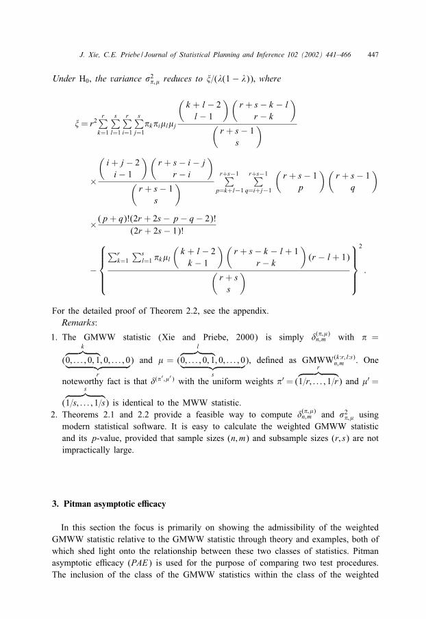
Under H0; the variance (2�;� reduces to )=('(1 − ')); where

) = r2r∑

k=1

s∑l=1

r∑i=1

s∑j=1

�k�i�l�j

(k + l− 2l− 1

)(r + s− k − l

r − k

)(

r + s− 1s

)

×

(i + j − 2i − 1

)(r + s− i − j

r − i

)(

r + s− 1s

) r+s−1∑p=k+l−1

r+s−1∑q=i+j−1

(r + s− 1

p

)(r + s− 1

q

)

× (p + q)!(2r + 2s− p− q− 2)!(2r + 2s− 1)!

−

∑r

k=1

∑sl=1 �k�l

(k + l− 2k − 1

)(r + s− k − l + 1

r − k

)(r − l + 1)(

r + ss

)

2

:

For the detailed proof of Theorem 2.2, see the appendix.Remarks:

1. The GMWW statistic (Xie and Priebe, 2000) is simply �(�;�)n;m with � =

(

k︷︸︸︷0; : : : ; 0; 1; 0; : : : ; 0︸︷︷︸

r

) and � = (

l︷︸︸︷0; : : : ; 0; 1; 0; : : : ; 0︸︷︷︸

s

), deGned as GMWW(k:r; l:s)n;m . One

noteworthy fact is that �(�′ ;�′) with the uniform weights �′ = (

r︷︸︸︷1=r; : : : ; 1=r) and �′ =

(

s︷︸︸︷1=s; : : : ; 1=s) is identical to the MWW statistic.

2. Theorems 2.1 and 2.2 provide a feasible way to compute �(�;�)n;m and (2

�;� usingmodern statistical software. It is easy to calculate the weighted GMWW statisticand its p-value, provided that sample sizes (n; m) and subsample sizes (r; s) are notimpractically large.

3. Pitman asymptotic e�cacy

In this section the focus is primarily on showing the admissibility of the weightedGMWW statistic relative to the GMWW statistic through theory and examples, both ofwhich shed light onto the relationship between these two classes of statistics. Pitmanasymptotic e5cacy (PAE) is used for the purpose of comparing two test procedures.The inclusion of the class of the GMWW statistics within the class of the weighted


GMWW statistics as stated in Theorem 3.1 implies that the Grst class is at most asgood as the second in the sense of the maximum PAE possible within each class.The e5cacy analysis result presented in this investigation indicates nontrivial gain ine5cacy using the optimal WGMWW statistics in the sense of PAE when the underlyingdensities are far from unimodal.

Pitman asymptotic e5cacy (PAE) is deGned in our case as

PAE (�(�;�)) =

[{dd�

�(�;�)�

}2∣∣∣∣∣�→�0

]/(2�;�;

where F = F�0 and G = F�, with � = �0 + c=n1=2 and where (2�;� is the null variance

given in Theorem 2.2. Applying this deGnition we see that for the location problemG(x) = F(x − �), under the assumption the density of F exists and is equal to f,

dd�

�(�;�)�

∣∣∣∣�→0

=r∑

k=1

s∑l=1

�k�lr!s!(k − 1)!(r − k)!(l− 1)!(s− l)!

×∫ ∞

−∞Fk+l−2(1 − F)r+s−k−lf2(x) dx:

Apparently, the explicit expressions for the PAE are not easy to derive in generaldue to the complexity of distribution functions. Hence we study the PAEs for variouscanonical types of distributions and therefore indicate the strengths and weaknesses ofthe WGMWW statistics. For simplicity, PAEs presented here are scaled by the constant'(1 − ').

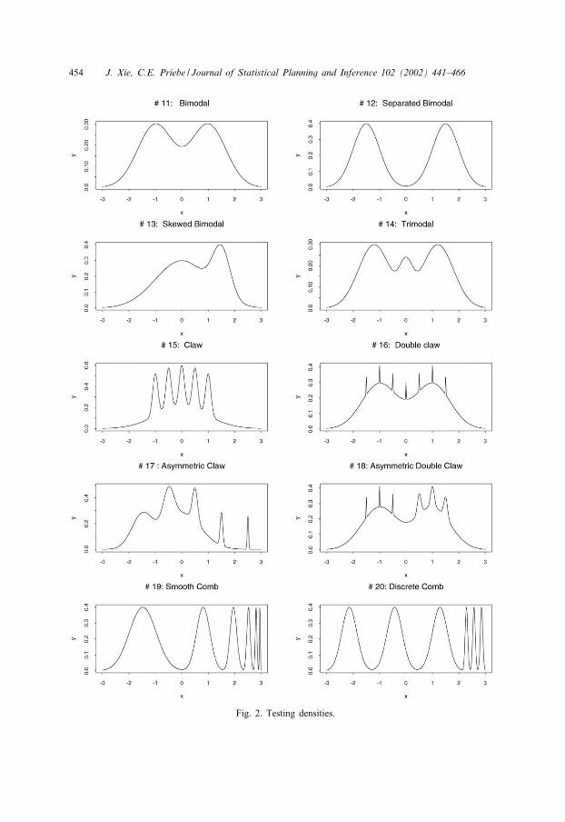
Twenty typical densities have been carefully chosen to investigate the overall perfor-mance of the WGMWW statistics in terms of PAE. Standard distributions consideredhere are the Uniform, Exponential, Logistic, Double Exponential and Cauchy distribu-tions. In addition, a test suite of 15 normal mixture densities (Marron and Wand, 1992)are included to represent a wide range of density shape. (Any density can be approxi-mated arbitrarily closely in various senses by a normal mixture.) Density numbers 1–10represent unimodal densities. The rest of the densities are multimodal. Density numbers1–6 are symmetric and unimodal, ranging from the heavy tail to the light tail whilethe skewness of the unimodal densities are increasing from number 7 to number 10.On the other hand, the density numbers 11–15 are mildly multimodal. The remainingdensities are strongly multimodal. We believe these densities eCectively model manyreal data situations.

Let us denote by Cr;s the class of two-sample GMWW statistics with subsample sizesr and s and denote by WCr;s the class of two-sample weighted GMWW statistics withsubsample sizes r and s. Clearly the fact that Cr;s ⊂ WCr;s leads to the conclusionthat the maximum PAE of the GMWW statistic in Cr;s is not greater than that inWCr;s. To prove the admissibility of the weighted GMWW statistic with respect tothe GMWW statistic, we need to show that Cr;s ⊂ WCr′ ; s′ , whenever r6r′ and s6s′

and hence the maximum PAE of the WGMWW statistic in WCr′ ; s′ is not less than


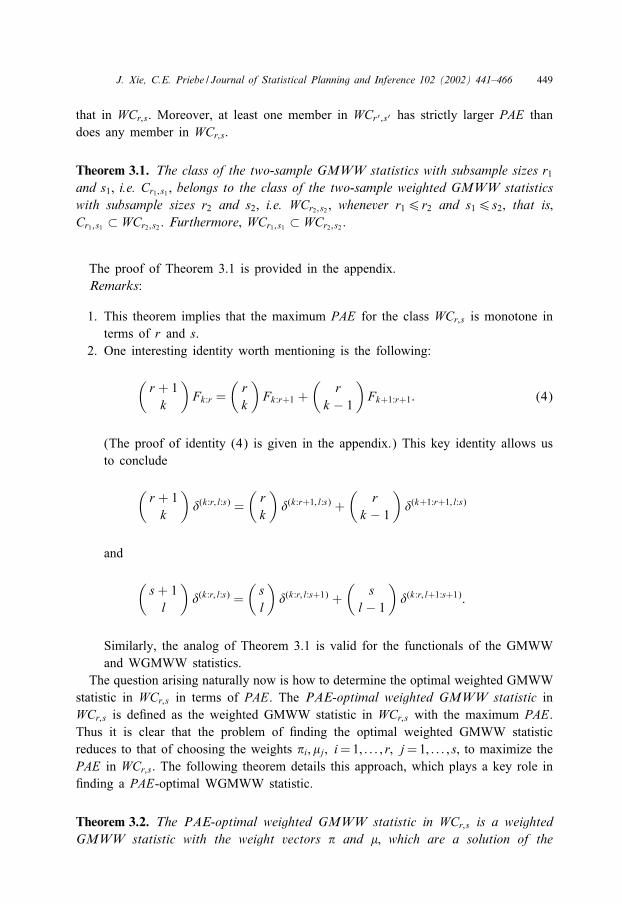
that in WCr;s. Moreover, at least one member in WCr′ ; s′ has strictly larger PAE thandoes any member in WCr;s:

Theorem 3.1. The class of the two-sample GMWW statistics with subsample sizes r1

and s1; i.e. Cr1 ; s1 ; belongs to the class of the two-sample weighted GMWW statisticswith subsample sizes r2 and s2; i.e. WCr2 ; s2 ; whenever r16r2 and s16s2; that is;Cr1 ; s1 ⊂ WCr2 ; s2 . Furthermore; WCr1 ; s1 ⊂ WCr2 ; s2 .

The proof of Theorem 3.1 is provided in the appendix.Remarks:

1. This theorem implies that the maximum PAE for the class WCr;s is monotone interms of r and s.

2. One interesting identity worth mentioning is the following:

(r + 1k

)Fk:r =

(rk

)Fk:r+1 +

(r

k − 1

)Fk+1:r+1: (4)

(The proof of identity (4) is given in the appendix.) This key identity allows usto conclude

(r + 1k

)�(k:r; l:s) =

(rk

)�(k:r+1; l:s) +

(r

k − 1

)�(k+1:r+1; l:s)

and

(s + 1l

)�(k:r; l:s) =

(sl

)�(k:r; l:s+1) +

(s

l− 1

)�(k:r; l+1:s+1):

Similarly, the analog of Theorem 3.1 is valid for the functionals of the GMWWand WGMWW statistics.

The question arising naturally now is how to determine the optimal weighted GMWWstatistic in WCr;s in terms of PAE. The PAE-optimal weighted GMWW statistic inWCr;s is deGned as the weighted GMWW statistic in WCr;s with the maximum PAE.Thus it is clear that the problem of Gnding the optimal weighted GMWW statisticreduces to that of choosing the weights �i; �j; i = 1; : : : ; r; j = 1; : : : ; s; to maximize thePAE in WCr;s. The following theorem details this approach, which plays a key role inGnding a PAE-optimal WGMWW statistic.

Theorem 3.2. The PAE-optimal weighted GMWW statistic in WCr;s is a weightedGMWW statistic with the weight vectors � and �; which are a solution of the


nonlinear programming problem with linear constraints as follows:

max’2(r; s; �; �))(r; s; �; �)

s:t:

∑ri=1 �i = 1;∑sj=1 �j = 1;

�i¿0; i = 1; : : : r;

�j¿0; j = 1; : : : s;

(5)

where )(r; s; �; �) is the null variance given in Theorem 3:1 and

’(r; s; �; �) =r∑

k=1

s∑l=1

r!s!�k�l∫∞−∞ Fk+l−2(1 − F)r+s−k−lf2(x) dx

(k − 1)!(r − k)!(l− 1)!(s− l)!:

If F(x) is a cumulative distribution with :nite Fisher information; then there existsa solution to (5).

Remarks:

1. The proof follows easily from the fact that given the distribution function F , thePAE or the objective function in (5) is bounded by the Fisher information of F .

2. There are many nonlinear programming software packages containing rich maxi-mization procedures which can be easily applied to choose the weights � and �.

3. Given that the density function f and distribution function F are unknown, anadaptive procedure may be necessary. If large samples are available, a nonparametricestimate for f and an empirical distribution for F may be applicable. This yieldsan adaptive procedure (Hogg et al., 1975). In fact, one of the major advantages ofthe weighted GMWW statistic is to take advantage of relatively large samples inorder to increase the PAE. Thus it is highly preferable in this scenario. However,application of an adaptive procedure in practice will not be addressed herein.

When the population distributions are assumed to diCer only in location, the MWWtest is directly comparable with the Student t-test which is known to be optimal withPAE of 1 under the assumption of normality. It is well known that if the populationdistributions are normal, the PAE of MWW is quite high at 0.955 (see Table 4 ofXie and Priebe, 2000). In fact, the overall PAE-optimal GMWW statistic is indeedthe MWW statistic. It is no wonder that many statisticians thus far have consideredthe MWW test to be an appropriate nonparametric test for the two-sample locationproblem in the case of F normal. In the following example, we Gnd that the WGMWWdominates the MWW for this case.

Example I. Assume F(x) to be the normal distribution function (our density # 4).Applying Theorem 3.2 and using the computer code in Appendix A of Xie (1999) for


solving (5) with r = s = 2, we obtain the solution

�1 = 0:5; �2 = 0:5; �1 = 0:5; �2 = 0:5;

which is in fact the classical MWW statistic. Notice that

0:5F1:2(x) + 0:5F2:2(x) = F(x)

and hence that

�(0:5;0:5;0:5;0:5) =∫ ∞

−∞{0:5F1:2(x) + 0:5F2:2(x)} d{0:5G1:2(x) + 0:5G2:2(x)}

=∫ ∞

−∞F(x) dG(x)

= �(1;1):

This is an illustrative example of Theorem 3.1, in which C1;1 ⊂ WC2;2. Furthermore,it appears that the maximum PAE of WC2;2 is equal to the maximum PAE of C1;1,0.955. On the other hand, the solution of (5) with r = s = 3 is

�1 = 0:5; �2 = 0; �3 = 0:5; �1 = 0:5; �2 = 0; �3 = 0:5

and thus the functional associated with this weighted GMWW statistic is

�(0:5;0;0:5;0:5;0;0:5) =∫ ∞

−∞{0:5F1:3(x) + 0:5F3:3(x)} d{0:5G1:3(x) + 0:5G3:3(x)};

which yields the PAE of 0.9891. Clearly the maximum PAE of the WGMWW statisticin WC3;3 is greater than that in WC2;2. It is also greater than the maximum PAE in C3;3

as shown in Table 1. Moreover, the maximum PAE for WCr;s; r=s=4; 5; 6 are 0.9932,0.9936, 0.9958, respectively. Experimentally, the maximum PAE for WCr;s increasesas r and s grow. This observation not only conforms to Theorem 3.1 as expected, butalso demonstrates the admissibility of WCr;s relative to Cr;s in terms of PAE.

Example II. Let us consider the Bimodal distribution F(x) (our density # 11). Bysolving (5) with r = s = 2; 3; 4; 5; 6, we obtain the weight vectors as follows:

�1 = �1 = �r = �r = 0:5 and �i = �i = 0; i = 2; : : : ; r − 1:

Hence the associated functional is

�(�;�) =∫ ∞

−∞{0:5F1:r(x) + 0:5Fr:r(x)} d{0:5F1:r(x) + 0:5Fr:r(x)}:

As displayed in Table 1, the maximum PAE for WCr;s is constantly increasing withsubsample sizes r and s. Most importantly, the gain in e5cacy using the PAE-optimalweighted GMWW statistic is substantial.

The PAE-optimal weighted GMWW statistic outperforms the PAE-optimal GMWWstatistic, as shown from Table 1. Regardless of the underlying distribution, the


Table 1Comparison of the WGMWW and GMWW statisticsa

ARE(WGMWW, GMWW)# r = s = 1 r = s = 2 r = s = 3 r = s = 4 r = s = 5 r = s = 6 Optimal(r; s)

#1 1 1 1 1 1 1 1#2 1 1 1 1 1 1 1#3 1 1.012 1.028 1.044 1.057 1.074 1#4 1 1.054 1.133 1.168 1.215 1.216 1.042#5 1 1 1 1 1 1 1#6 1 1 1.006 1.021 1.036 1.048 1.007#7 1 1 1 1 1 1 1#8 1 1 1 1 1 1 1#9 1 1.016 1.045 1.075 1.081 1.1 1.027

#10 1 1 1 1 1 1 1#11 1 1.050 1.248 1.476 1.6 1.667 1.615#12 1 1.007 1.193 1.440 1.585 1.664 1.635#13 1 1 1 1 1.121 1.145 1.136#14 1 1.024 1.217 1.451 1.588 1.667 1.657#15 1 1.079 1.283 1.5 1.554 1.516 1.516#16 1 1.049 1.249 1.439 1.594 1.674 1.626#17 1 1.008 1.147 1.310 1.413 1.481 1.481#18 1 1 1.107 1.297 1.418 1.449 1.425#19 1 1 1.131 1.263 1.123 1.299 1.299#20 1 1 1.163 1.389 1.497 1.532 1.532

aARE(WGMWW;GMWW) = max PAE(WGMWW∈WCr; s)max PAE(GMWW∈Cr; s)

.

PAE-optimal WGMWW statistic always has a nondecreasing PAE in terms of subsam-ple sizes r and s. In contrast, this is not generally true for the PAE-optimal GMWWstatistic. As far as the unimodal densities number 1 to number 10 are concerned, itis clear that under the Gaussian, Outlier, Logistic and Skewed unimodal distributions,the PAE-optimal weighted GMWW statistic gains higher e5cacy than its counterpartin the class of the GMWW statistics, i.e. the corresponding PAE-optimal GMWWstatistic (Fig. 1). This indicates the admissibility of the WGMWW statistic relativeto the GMWW statistic. In fact, the former dominates the latter; we observe that thePAE-optimal weighted GMWW statistic is at least as good as the PAE-optimal GMWWstatistic for the remaining unimodal densities. As for PAE analyses of the multimodaldensities displayed in Table 1 (density numbers 11–20), the PAE-optimal weightedGMWW statistic shows substantial improvement over the PAE-optimal GMWW statis-tic (Fig. 2). For example, for r = s = 6, the PAE-optimal weighted GMWW statisticgives rise to almost 65:7% increase in e5cacy over the PAE-optimal GMWW statisticfor the density # 14. Overall, the superiority of the former over the latter thereforebecomes apparent as anticipated from Theorem 3.1. It is highly recommended that thePAE-optimal WGMWW statistic be used, especially when the underlying distributionis multimodal, as opposed to the PAE-optimal GMWW statistic.


Fig. 1. Testing densities.


Fig. 2. Testing densities.


4. One-sample analog: a weighted generalization of the Wilcoxon signed rankstatistic

Analogous to the two-sample case, a class of weighted generalizations of the Wilcoxonsigned rank (WSR) statistics is introduced for testing the center of a symmetric dis-tribution, including as special cases the Wilcoxon Signed Rank, the Maesono–Ahmad(Maesono, 1987; Ahmad, 1996) and the GWSR (Xie and Priebe, 2000) statistics.

As in the two-sample case, Lemmas 1.1 and 1.2 motivate us to estimate the functional�(�;�) deGned as

�(�;�) =∫ ∞

−∞

r∑k=1

�kbk:r{1 − F(−x)} d[

s∑l=1

�lbl:s{F(x)}]

=∫ ∞

−∞

r∑k=1

�k JFr−k+1:r(−x) d{

s∑l=1�lFl:s(x)

}

=r∑

k=1

s∑l=1

�k�l

∫ ∞

−∞JFr−k+1:r(−x) dFl:s(x)

=r∑

k=1

s∑l=1

�k�lPr{Xk:r(X1; : : : ; Xr) + Xl:s(Xr+1; : : : ; Xr+s)¿0};

where JFr−k+1:r(−x) =∑r

v=r−k+1( rv ) JF

v(−x)(1 − JF(−x))r−v and � = (�1; : : : ; �r) and

� = (�1; : : : ; �s) are the weight vectors and where X1; : : : ; Xr are r independent copiesof X and X1:r ; : : : ; Xr:r are the order statistics obtained by arranging the precedingrandom sample in increasing order of magnitude. Notice that under H0, �(�;�) =

∑rk=1∑s

l=1 �k�l∑r

i=r−k+1 ( l+i−1i )( s+r−i−l

r−i )=( r+sr ).

An empirical estimate of �(�;�) is given by

�(�;�)n =

{(n

r + s

)(r + ss

)}−1 ∑C

r∑k=1

s∑l=1

�k�lI{Xk:r(Xi1 ; : : : ; Xir ) + Xl:s(Xir+1 ; : : : ; Xir+s)¿0}

=

∑rk=1

∑sl=1

∑n−r+ki=k

∑n−s+lj=l �k�lwijI(Xi:n + Xj:n¿0)(

nr + s

)(r + sr

) ;

where∑

c stands for summation over all permutations (i1; : : : ; ir+s) of r + s integerssuch that 16 i1¡ · · ·¡ir6n, 16 ir+1¡ · · ·¡ir+s6n, and ie �= if if e �= f, 16e6rand 16f6s, and where

wij =

∑l−1v=0

(i − 1k − 1

)(i − kv

)(j − i − 1l− v− 1

)(n− js− l

)(n + v− i − s

r − k

)i¡j;

0 i = j;∑s−lv=0

(j − 1l− 1

)(i − j − l

v

)(n− i − r + k

s− l− v

)(n− ir − k

)(i − l− v− 1

k − l

)i¿j:


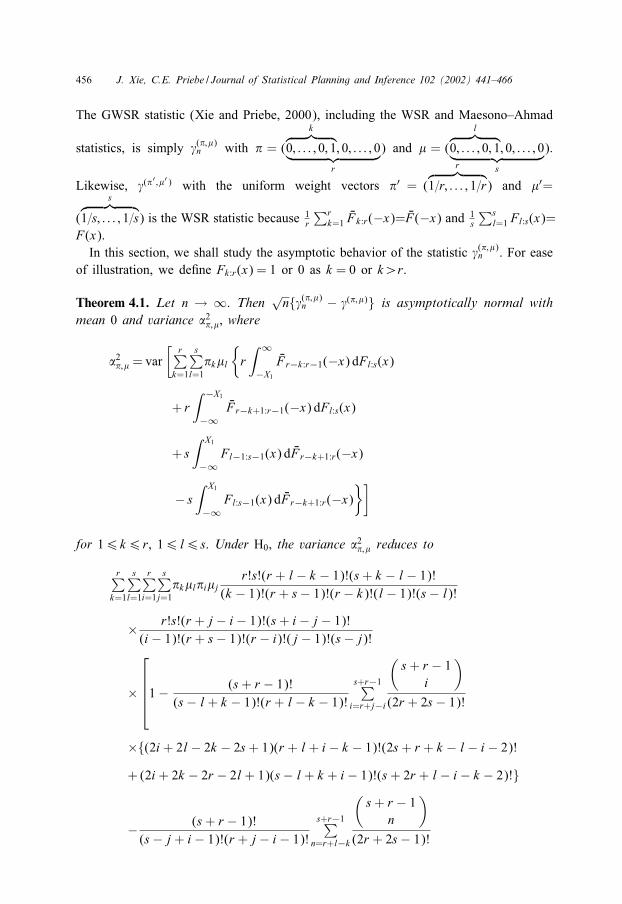
The GWSR statistic (Xie and Priebe, 2000), including the WSR and Maesono–Ahmad

statistics, is simply �(�;�)n with � = (

k︷︸︸︷0; : : : ; 0; 1; 0; : : : ; 0︸︷︷︸

r

) and � = (

l︷︸︸︷0; : : : ; 0; 1; 0; : : : ; 0︸︷︷︸

s

).

Likewise, �(�′ ;�′) with the uniform weight vectors �′ = (

r︷︸︸︷1=r; : : : ; 1=r) and �′=

(

s︷︸︸︷1=s; : : : ; 1=s) is the WSR statistic because 1

r

∑rk=1

JFk:r(−x)= JF(−x) and 1s

∑sl=1 Fl:s(x)=

F(x).In this section, we shall study the asymptotic behavior of the statistic �(�;�)

n . For easeof illustration, we deGne Fk:r(x) = 1 or 0 as k = 0 or k¿r.

Theorem 4.1. Let n → ∞. Then√n{�(�;�)

n − �(�;�)} is asymptotically normal withmean 0 and variance 02

�;�; where

02�;� = var

[r∑

k=1

s∑l=1

�k�l

{r∫ ∞

−X1

JFr−k:r−1(−x) dFl:s(x)

+ r∫ −X1

−∞JFr−k+1:r−1(−x) dFl:s(x)

+ s∫ X1

−∞Fl−1:s−1(x) d JFr−k+1:r(−x)

− s∫ X1

−∞Fl:s−1(x) d JFr−k+1:r(−x)

}]

for 16k6r, 16l6s. Under H0; the variance 02�;� reduces to

r∑k=1

s∑l=1

r∑i=1

s∑j=1

�k�l�i�jr!s!(r + l− k − 1)!(s + k − l− 1)!

(k − 1)!(r + s− 1)!(r − k)!(l− 1)!(s− l)!

× r!s!(r + j − i − 1)!(s + i − j − 1)!(i − 1)!(r + s− 1)!(r − i)!(j − 1)!(s− j)!

×

1 − (s + r − 1)!

(s− l + k − 1)!(r + l− k − 1)!

s+r−1∑i=r+j−i

(s + r − 1

i

)(2r + 2s− 1)!

×{(2i + 2l− 2k − 2s + 1)(r + l + i − k − 1)!(2s + r + k − l− i − 2)!

+ (2i + 2k − 2r − 2l + 1)(s− l + k + i − 1)!(s + 2r + l− i − k − 2)!}

− (s + r − 1)!(s− j + i − 1)!(r + j − i − 1)!

s+r−1∑n=r+l−k

(s + r − 1

n

)(2r + 2s− 1)!


×{(2n + 2j − 2i − 2s + 1)(r + j + n− i − 1)!(2s + r + i − j − n− 2)!

+ (2n + 2i − 2r − 2j + 1)(s− j + i + n− 1)!(s + 2r + j − n− i − 2)!}

:

Thus the proof of Theorem 4.1 is similar to that of Theorem 3.1.Let us denote by Vr;s the class of the one-sample GWSR statistics with subsample

sizes r and s and denote by WVr;s the class of the one-sample weighted GWSR statisticswith subsample sizes r and s. Apparently, Vr;s ⊂ WVr;s. As in the two-sample case,we have the following theorem characterizing the relationship between the classes Vand WV .

Theorem 4.2. The class of the one-sample GWSR statistics with subsample sizesr1 and s1; i.e. Vr1 ; s1 ; is included in the class of the one-sample weighted GWSRstatistics with subsample sizes r2 and s2; i.e. WVr2 ; s2 ; whenever r16r2 and s16s2;that is; Vr1 ; s1 ⊂ WVr2 ; s2 : Furthermore; WVr1 ; s1 ⊂ WVr2 ; s2 .

The PAE-optimal weighted GWSR statistic in WVr;s is deGned as the weightedGWSR statistic with the maximum e5cacy in WVr;s. The problem of Gnding the optimalweighted GWSR statistic reduces to that of choosing the weights �i; �j; i=1; : : : ; r; j=1; : : : ; s to maximize the PAE of the WGWSR statistic in WVr;s.

Theorem 4.3. Suppose that the cumulative distribution F(x) is known. A PAE-optimalweighted GWSR statistic in WVr;s is the weighted GWSR statistic with weight vec-tors � and �; which are a solution of the nonlinear programming problem with linearconstraints as follows:

max!2(r; s; �; �) (r; s; �; �)

s:t:

∑ri=1 �i = 1;∑sj=1 �j = 1;

�i¿0; i = 1; : : : r;

�j¿0; j = 1; : : : s;

(6)

where (r; s; �; �) is the null variance given by Theorem 4:1 and

!(r; s; �; �) =r∑

k=1

s∑l=1

2r!s!�k�l∫∞−∞ Fr−k+l−1(1 − F)s+k−l−1f2(x) dx

(k − 1)!(r − k)!(l− 1)!(s− l)!:

If the Fisher information of F(·) is bounded; then there exists a solution to (6:15):

Proof. The proof follows from the similar argument in the proof of Theorem 3.2.


Example I. Suppose that F(x) is the normal distribution function. Applying Theorem4.3 and using the computer code in Appendix B of Xie (1999) for solving (6), weobtain the maximum PAEs for WVr;s; r = s = 2; 3; 4; 5; 6; which are 0.9760, 0.9896,0.9932, 0.9937 and 0.9959, respectively. As subsample sizes r; s get large, the optimalPAE increases. This agrees with Theorem 4.2. Notice that for the normal distribution,the maximum achievable PAE is 1. Since the one-sample t-test with PAE=1 is optimalfor the normal distribution, the PAE-optimal WGWSR with r = s = 6 is a strongnonparametric competitor.

Appendix

Proof of Lemma 1.1. It is su5cient to consider the case in which u(0)=0 and u(1)=1.Suppose that u(x) is a strictly increasing continuous function on [0; 1] and that u(0)=0and u(1) = 1. In light of the Weierstrass approximation theorem (Theorem 1:1:1 ofLorentz (1986)), this implies that the Bernstein polynomials ur(x) of the function u(x)converges to u(x) uniformly on [0; 1]: Moreover, ur(x) can be expressed in terms ofthe tail binomial polynomials bk:r(x); k = 1; : : : ; r. To see this, let us take a closer lookat ur(x).

ur(x) =r∑

k=0u(kr

)( rk

)xk(1 − x)r−k

= u(1)br:r(x) +r−1∑k=0

u(kr

){bk:r(x) − bk+1:r(x)}

= u(0)b0:r(x) +r∑

k=1

{u(kr

)− u

(k − 1

r

)}bk:r(x)

=r∑

k=1

{u(kr

)− u

(k − 1

r

)}bk:r(x)

=r∑

k=1wkbk:r(x);

where wk = u(k=r) − u((k − 1)=r)¿0; k = 1; : : : ; r and∑r

k=1 wk = 1. The proof iscompleted as desired.

Proof of Lemma 1.2. It is su5cient to show that∫ 1

0ur(x) dvs(x) →

∫ 1

0u(x) dv(x) as r; s → ∞ and r=s → ' ∈ (0; 1):

Without loss of generality, we are assuming that u(0)=0, and hence 0¡u(1)¡∞: Thecontinuity of v′, taken together with the Weierstrass approximation theorem, impliesthat the Bernstein polynomials of v′(x), i.e. v′s(x), converge to v′(x) uniformly on [0; 1].Thus, for any 3¿0, and all x ∈ [0; 1], there exists M ′ such that |v′s(x)−v′(x)|¡3=2u(1),whenever s¿M ′. Once again, it follows from the Weierstrass approximation theorem


that ur(x) and vs(x) converge to u(x) and v(x) uniformly on [0; 1], respectively. Thisimplies that for any 0¡3¡1 and all x ∈ [0; 1], there exist N1 and M1 such that|ur(x)−u(x)|¡3=2(2+|v(1)−v(0)|) and |vs(x)−v(x)|¡3; whenever r¿N1 and s¿M1.All in all, for any 3¿0, there exists M = max{N1; M1; M ′} such that∣∣∣∣∣

∫ 1

0ur(x) dvs(x) −

∫ 1

0u(x) dv(x)

∣∣∣∣∣=

∣∣∣∣∣∫ 1

0{ur(x) − u(x)} dvs(x) +

∫ 1

0u(x) d{vs(x) − v(x)}

∣∣∣∣∣6

∣∣∣∣∣∫ 1

0{ur(x) − u(x)} dvs(x)

∣∣∣∣∣ +

∣∣∣∣∣∫ 1

0u(x) d{vr(x) − v(x)}

∣∣∣∣∣6

∫ 1

0|ur(x) − u(x)| dvs(x) +

∫ 1

0|u(x){v′s(x) − v′(x)}| dx

6|vs(1) − vs(0)|3

2(2 + |v(1) − v(0)|) + |u(1)|∫ 1

0|v′s(x) − v′(x)| dx:

Hence the lemma follows as desired.

Proof of Theorem 2.2. Using Theorem 3:4:13 of Randles and Wolfe (1979), we needonly to establish the variance. Let

’(�;�)(X1; : : : ; Xr;Y1; : : : ; Ys) =r∑

k=1

s∑l=1

�k�lI{Xk:r(X1; : : : ; Xr)¡Yl:s(Y1; : : : ; Ys)}:

Thus

’(�;�)10 (X1) = E[’(�;�)(X1; : : : ; Xr;Y1; : : : ; Ys)|X1]

=r∑

k=1

s∑l=1

�k�l Pr{Xk:r(X1; : : : ; Xr)6Yl:s(Y1; : : : ; Ys)|X1}

=r∑

k=1

s∑l=1

�k�lPr{Xk:r6Yl:s|X1}

=r∑

k=1

s∑l=1

�k�l’(k:r; l:s)10 (X1):

Similarly, we have

’(�;�)01 (Y1) = E{’(�;�)(X1; : : : ; Xr;Y1; : : : ; Ys)|Y1}

=r∑

k=1

s∑l=1

�k�l Pr{Xk:r6Yl:s|Y1}

=r∑

k=1

s∑l=1

�k�l’(k:r; l:s)01 (Y1):


Under H0;

E’(�;�)10 (X1) = E’(�;�)

01 (Y1)

=r∑

k=1

s∑l=1

�k�lE’(k:r; l:s)01 (Y1)

= �(�;�)

=(

r + sr

)−1 r∑k=1

s∑l=1

�k�l

r∑i=k

(l + i − 1

i

)(r + s− i − l

r − i

):

)1;0 = var{’(�;�)10 (X1)}

= var{

r∑k=1

s∑l=1

�k�l

∫ X1

−∞(Fk:r−1 − Fk−1:r−1)(x) dFl:s(x)

}

= E{

r∑k=1

s∑l=1

�k�l

∫ X1

−∞(Fk:r−1 − Fk−1:r−1)(x) dFl:s(x)

}2

−E2{

r∑k=1

s∑l=1

�k�l

∫ X1

−∞(Fk:r−1 − Fk−1:r−1)(x) dFl:s(x)

}

= A− B2;

where

B = E{

r∑k=1

s∑l=1

�k�l

∫ X1

−∞(Fk:r−1 − Fk−1:r−1)(x) dFl:s(x)

}

=r∑

k=1

s∑l=1

�k�lE{∫ X1

−∞(Fk:r−1 − Fk−1:r−1)(x) dFl:s(x)

}

=

∑rk=1

∑sl=1 �k�l

(k + l− 2k − 1

)(r + s− k − l + 1

r − k

)(r − l + 1)

r(

r + ss

)

and

A = E{

r∑k=1

s∑l=1

�k�l

∫ X1

−∞(Fk:r−1 − Fk−1:r−1)(x) dFl:s(x)

}2

=r∑

k=1

s∑l=1

r∑i=1

s∑j=1

�k�i�l�jE{∫ X1

−∞(Fk:r−1 − Fk−1:r−1)(x) dFl:s(x)

×∫ X1

−∞(Fi:r−1 − Fi−1:r−1)(x) dFj:s(x)

}


=r∑

k=1

s∑l=1

r∑i=1

s∑j=1

�k�i�l�j

(k + l− 2l− 1

)(r + s− k − l

r − k

)(

r + s− 1s

)

×

(i + j − 2i − 1

)(r + s− i − j

r − i

)(

r + s− 1s

)

×r+s−1∑

p=k+l−1

r+s−1∑q=i+j−1

(r + s− 1

p

)(r + s− 1

q

)E{Fp+q(1 − F)2r+2s−p−q−2}

=r∑

k=1

s∑l=1

r∑i=1

s∑j=1

�k�i�l�j

(k + l− 2l− 1

)(r + s− k − l

r − k

)(

r + s− 1s

)

×

(i + j − 2i − 1

)(r + s− i − j

r − i

)(

r + s− 1s

)

×r+s−1∑

p=k+l−1

r+s−1∑q=i+j−1

(r+s−1

p

)(r+s−1

q

)(p + q)!(2r+2s−p−q−2)!

(2r+2s−1)!:

Similarly

)0;1 = var{’(�;�)0;1 (Y1)}

= var{

r∑k=1

s∑l=1

�k�l

∫ X1

−∞(Fl:s−1 − Fl−1:s−1)(x) dFk:r(x)

}

= E{

r∑k=1

s∑l=1

�k�l

∫ X1

−∞(Fl:s−1 − Fl−1:s−1)(x) dFk:r(x)

}2

−E2

r∑

k=1

s∑l=1

�k�l

X1∫−∞

(Fl:s−1 − Fl−1:s−1) dFk:r(x)

= C − D2;


where

D = E{

r∑k=1

s∑l=1

�k�l

∫ X1

−∞(Fl:s−1 − Fl−1:s−1) dFk:r(x)

}

=r∑

k=1

s∑l=1

�k�lE{∫ X1

−∞(Fl:s−1 − Fl−1:s−1) dFk:r(x)

}

=

∑rk=1

∑sl=1�k�l

(k + l− 2l− 1

)(r + s− k − l + 1

s− l

)(s− k + 1)

s(

r + sr

)and

C =r∑

k=1

s∑l=1

r∑i=1

s∑j=1

�k�i�l�j

(k + l− 2k − 1

)(r + s− k − l

s− l

)(

r + s− 1r

)

×

(i + j − 2j − 1

)(r + s− i − j

s− j

)(

r + s− 1r

)

×r+s−1∑

p=k+l−1

r+s−1∑q=i+j−1

(r+s−1

p

)(r+s−1

q

)(p + q)!(2r+2s−p−q−2)!

(2r+2s−1)!:

Thus r2)1;0=' + s2)0;1=(1 − ') is identical to the variance under H0, i.e. )=('(1 − ')).

Proof of Theorem 3.1. Firstly, we claim that(r + 1k

)GMWW(k:r; l:s)

n;m =(

rk

)GMWW(k:r+1; l:s)

n;m

+(

rk − 1

)GMWW(k+1:r+1; l:s)

n;m : (7)

Since (r + 1k

)GMWW(k:r; l:s)

n:m

=

(r + 1k

)∑ni=1

∑mj=1

(i − 1k − 1

)(n− ir − k

)(j − 1l− 1

)(m− js− l

)I(Xi:n¡Yj:m)(

nr

)(ms

) ;


(rk

)GMWW(k:r+1; l:s)

n;m

=

(rk

)∑ni=1

∑mj=1

(i − 1k − 1

)(n− i

r − k + 1

)(j − 1l− 1

)(m− js− l

)I(Xi:n¡Yj:m)(

nr + 1

)(ms

)

and

(r

k − 1

)GMWW(k+1:r+1; l:s)

n;m

=

(r

k − 1

)∑ni=1

∑mj=1

(i − 1k

)(n− ir − k

)(j − 1l− 1

)(m− js− l

)I(Xi:n¡Yj:m)(

nr + 1

)(ms

) ;

it is su5cient to show that

(r + 1k

)(i − 1k − 1

)(n− ir − k

)(

nr

) =

(r

k − 1

)(i − 1k

)(n− ir − k

)(

nr + 1

)

+

(rk

)(i − 1k − 1

)(n− i

r − k + 1

)(

nr + 1

) :

By expanding and simplifying both sides, this identity follows immediately. Likewise,we obtain

(s + 1l

)GMWW(k:r; l:s)

n;m =(

sl

)GMWW(k:r; l:s+1)

n:m +(

sl− 1

)GMWW(k:r; l+1:s+1)

n;m :

(8)

Secondly, combining (7) and (8) yields

GMWW(k:r; l:s)n;m


=

(rk

){(sl

)GMWW(k:r+1; l:s+1)

n;m +(

sl− 1

)GMWW(k:r+1; l+1:s+1)

n;m

}(

r + 1k

)(s + 1l

)

+

(r

k − 1

){(sl

)GMWW(k+1:r+1; l:s+1)

n;m +(

sl− 1

)GMWW(k+1:r+1; l+1:s+1)

n;m

}(

r + 1k

)(s + 1l

) :

Hence (7) implies that

Cr;s ⊂ WCr+1; s ⇒ WCr;s ⊂ WCr+1; s

and (8) implies that

Cr;s ⊂ WCr;s+1 ⇒ WCr;s ⊂ WCr+1; s+1:

Finally, using the above recursive relations yields

Cr1 ; s1 ⊂ WCr1 ; s1 ⊂ WCr2 ; s2 ;

whenever r16r2 and s16s2.The proof of theorem is completed as desired.

Proof of Identity (4).

Fk:r =r∑

i=k

(ri

)Fi(1 − F)r−i

=r∑

i=k

(ri

){Fi(1 − F)r−i+1 + Fi+1(1 − F)r−i}

=r∑

i=k

(ri

)Fi:r+1 − Fi+1:r+1(

r + 1i

) +Fi+1:r+1 − Fi+2:r+1(

r + 1i + 1

)

=r∑

i=k

(ri

)(

r + 1i

)Fi:r+1 +

((r + 1

i

)−(

r + 1i + 1

))(ri

)(

r + 1i

)(r + 1i + 1

) Fi+1:r+1

−

(ri

)(

r + 1i + 1

)Fi+2:r+1


=

(rk

)(

r + 1k

)Fk:r+1

+

{(r + 1k

)−(

r + 1k + 1

)}(rk

)+(

r + 1k

)(r

k + 1

)(

r + 1k

)(r + 1k + 1

) Fk+1:r+1

+r−2∑i=k

−

(ri

)(

r + 1i + 1

) +

{(r + 1i + 1

)−(

r + 1i + 2

)}(r

i + 1

)(

r + 1i + 1

)(r + 1i + 2

)

+

(r

i + 2

)(

r + 1i + 2

)Fi+2:r+1

+

{(

r + 1r

)−(

r + 1r + 1

)}(rr

)(

r + 1r

)(r + 1r + 1

) −

(r

r − 1

)(

r + 1r

)Fr+1:r+1

=

(rk

)(

r + 1k

)Fk:r+1 +

(r

k − 1

)(

r + 1k

)Fk+1:r+1:

The proof is completed as desired.

References

Adams et al., 2000. Ahmad, I.A. (1996). A class of Mann–Whitney–Wilcoxon type statistics, The AmericanStatistician, 50, 324–327: Comment by Adams, Adams, Chang, Etzel, Kuo, Montemayor, and Schucany;and Reply. Amer. Statist. 54, 160.

Ahmad, I.A., 1996. A class of Mann–Whitney–Wilcoxon type statistics. Amer. Statist. 50, 324–327.Deshpande, J.V., Kochar, S.C., 1980. Some competitors of tests based on powers of ranks for the two-sample

problem. Sankhya Ser. B 42, 236–241.Hogg, R.V., Fisher, D.M., Randles, R.H., 1975. A two-sample adaptive distribution-free test. J. Amer. Statist.

Assoc. 70, 656–661.Kochar, S.C., 1978. A class of distribution-free tests for the two-sample slippage problem. Comm. Statist.

Theory Methods A 7 (13), 1243–1252.Kumar, N., 1997. A class of two-sample tests for location based on sub sample medians. Comm. Statist.

Theory Methods 26, 943–951.


Lorentz, G.G., 1986. Bernstein Polynomials, 2nd Edition. Chelsea, New York.Maesono, Y., 1987. Competitors of the Wilcoxon signed rank test. Ann. Inst. Statist. Math. 39, 363–375.Mann, H.B., Whitney, D.R., 1947. On a test of whether one of two random variables is stochastically larger

than the other. Ann. Math. Statist. 18, 50–60.Marron, J.S., Wand, M.P., 1992. Exact mean integrated squared error. Ann. Statist. 20, 712–736.Mathisen, H.C., 1943. A method of testing the hypothesis that two samples are from the same population.

Ann. Math. Statist. 14, 188–194.Priebe, C.E., Cowen, L.J., 1999. A generalized Wilcoxon–Mann–Whitney statistic. Comm. Statist. Theory

Methods 28 (12), 2871–2878.Randles, R.H., Wolfe, D.A., 1979. Introduction to the Theory of Nonparametric Statistics, Wiley Series in

Probability and Mathematical Statistics. Wiley, New York.Shetty, I.D., Bhat, S.V., 1994. A note on the generalization of Mathisen’s median test. Stat. Probab. Lett.

19, 199–204.Shetty, I.D., Govindarajulu, Z., 1988. A two-sample test for location. Comm. Statist. Theory Methods 17,

2389–2401.Stephenson, R.W., Ghosh, M., 1985. Two sample nonparametric tests based on subsamples. Comm. Statist.

Theory Methods 14 (7), 1669–1684.Wilcoxon, F., 1945. Individual comparisons by ranking methods. Biometrics 1, 80–83.Xie, J., 1999. Generalizing the Mann–Whitney–Wilcoxon statistic. Dissertation, The Johns Hopkins

University.Xie, J., Priebe, C.E., 2000. Generalizing the Mann–Whitney–Wilcoxon Statistic. J. Nonparametric Statist. 12,

661–682.

Documents

A weighted generalization of the …parky/CEP-Publications/XP-JSPI2002.pdfJournal of Statistical Planning and Inference 102 (2002) 441–466 A weighted generalization of the Mann–Whitney–WilcoxonPublished