A Water Quality Index for Ecology's Stream Monitoring Program

November 2002 Publication No. 02-03-052

A Water Quality Index for Ecology’s Stream Monitoring Program

Abstract

The Water Quality Index (WQI) presented here is a unitless number ranging from 1 to 100. A higher number is indicative of better water quality. For temperature, pH, fecal coliform bacteria and dissolved oxygen, the index expresses results relative to levels required to maintain uses according to criteria specified in WAC 173-201A. For nutrient and sediment measures, where standards are not specific, results are expressed relative to expected conditions in a given Ecoregion. Multiple constituents are combined and results aggregated over time to produce a single score for each sample station. In general, stations scoring 80 and above met expectations for water quality and are of "lowest concern," scores 40 to 80 indicate "marginal concern," and water quality at stations with scores below 40 did not meet expectations and are of "highest concern." A spreadsheet-version for calculating the WQI is available from the author. Monthly WQI scores are suitable for statistical trend analysis. Prior to adjusting for flow, statistically significant (p < 0.05) improving trends in overall (aggregated constituents) WQI scores were indicated at four stations and declining trends at one station out of 62 evaluated. Adjusting for flow increased the trend slope at nearly three quarters of the stations and resulted in statistically significant improving trends at nine stations and no declining trends. That is, trends in flow were apparently masking improving trends in overall WQI scores at many stations.

A D e p a r t m e n t o f E c o l o g y R e p o r t

2

Publication Information This report is available on the Department of Ecology home page on the World Wide Web at http://www.ecy.wa.gov/biblio/0203052.html For a printed copy of this report, contact the Department of Ecology Publications Distribution Office and ask for publication number 02-03-052

E-mail: [email protected] Phone: (360) 407-7472 Address: PO Box 47600, Olympia WA 98504-7600

Author: Dave Hallock Washington State Department of Ecology Environmental Assessment Program Phone: (360) 407-6681

Address: PO Box 47600, Olympia WA 98504-7600

The Department of Ecology is an equal-opportunity agency and does not discriminate on the basis of race, creed, color, disability, age, religion, national origin, sex, marital status, disabled-veteran’s status, Vietnam-era veteran’s status, or sexual orientation.

If you have special accommodation needs or require this document in alternative format, contact Michelle Harper at 360-407-6677 (voice) or 711 or 1-800-877-8973 (TTY).

3

Introduction Political decision-makers, non-technical water managers, and the general public usually have neither the time nor the training to study and understand a traditional, technical review of water quality data. A number of indexes have been developed to summarize water quality data in an easily expressible and easily understood format (Couillard and Lefebvre, 1985). Water quality professionals are frequently resistant to the automated, uncritical summarization represented by indexes, and there are good reasons to use the results of any index with caution (see the section on “Uses and Limitations”). "[Professionals] prefer to give no answer rather than an imperfect answer that could lead to misunderstanding. Yet the layman usually prefers an imperfect answer to no answer at all" (Ott, 1978). While the use of an index may not be the best way to understand large-scale water quality conditions, it is for many the only way. Professionals must understand the need for an imperfect answer and laymen must understand and accept the answer’s limitations. Ecology’s Freshwater Monitoring Unit’s Water Quality Index (WQI) is an attempt at an imperfect answer to non-technical questions about water quality. It is a unitless number ranging from 1 to 100; a higher number is indicative of better water quality. For temperature, pH, fecal coliform bacteria and dissolved oxygen, the index expresses results relative to levels required to maintain beneficial uses (based on criteria in Washington’s Water Quality Standards, WAC 173-201A). For nutrient and sediment measures, where standards are not specific, results are expressed relative to expected conditions in a given Ecoregion (Omernik and Gallant, 1986). Multiple constituents are combined and results aggregated over time to produce a single score for each sample station. In general, stations scoring 80 and above met expectations for water quality and are of "lowest concern," scores 40 to 80 indicate "marginal concern," and water quality at stations with scores below 40 did not meet expectations and are of "highest concern." A spreadsheet-version for calculating the WQI is available from the author. Acknowledgements Several people provided advice, review comments, or laid footprints in the sand for me to follow. In the latter category are all those people involved in developing the index used in the 1980s (in particular, Ray Peterson tickled some very old brain cells to respond to my questions), as well as those who worked on Oregon’s index (most recently, Curtis Cude). Several people offered suggestions on presentation; Bill Yake delved deeper than most into the mechanics. Besides offering innovative suggestions, Eric Aroner, as the only non-government employee involved, deserves special mention for his generosity in donating his time. I also want to recognize those people that provided comments and/or completed a survey on some of the more technical issues. Among these were Chad Wiseman, Nora Jewett, Jeanette Barreca, Dewey Weaver, Bill Ward, Curtis Cude, Jim Ross, Will Kendra, and William Ehinger.

4

Uses and Limitations Indexes by design contain less information than the raw data that they summarize; many uses of water quality data cannot be met with an index. An index is most useful for comparative purposes (what stations have particularly poor water quality?) and for general questions (how is water quality in my stream?). Indexes are less suited to specific questions. Site-specific decisions should be based on an analysis of the original water quality data. In short, an index is a useful tool for “communicating water quality information to the lay public and to legislative decision makers;” it is not “a complex predictive model for technical and scientific application” (McClelland, 1974). This index was developed as a tool to summarize and report our routine stream monitoring data to the public. Besides being general in nature (imprecise), there are at least two reasons that an index may fail to accurately communicate water quality information. First, most indexes are based on a pre-identified set of water quality constituents. For example, a particular station may receive a good WQI score, and yet have water quality impaired by constituents not included in the index. Second, aggregation of data may either mask (or over-emphasize) short-term water quality problems. A satisfactory WQI at a particular station does not necessarily mean that water quality was always satisfactory. A good score should, however, indicate that poor water quality (for evaluated constituents, at least) was not chronic during the period included in the index. Strategies Different approaches to indexing water quality results are possible. One approach is to rate quality objectively, for example, using ranked data (e.g., Harkins, 1974). While this approach does not require developing subjective rating curves, it does not permit comparisons between values generated from different data sets. For example, results between years could not be compared unless scores were re-calculated using data from all years. Anytime additional data are added and the index re-calculated (for example, to compare years), results for the same stations and dates originally evaluated will change if the rank order changes. Also, this approach ranks results from pristine stations where high quality would be expected along with stations where water quality would not be expected to be pristine (regardless of human impacts). Hence, a score could only be interpreted in comparison to some other station of known quality (which is in itself subjective). For management purposes, a more useful index is not one that merely ranks stations by relative water quality, but rather one that indicates whether water quality is less than expected or necessary to support uses designated for particular water bodies. There are disadvantages to this approach as well, however. This type of index requires subjective determinations of the beneficial uses that a particular stream segment should support, the level of water quality required to support those uses, and how critical a variation from that level of quality is. Another disadvantage is that, by design, this approach indicates how well water quality at a station meets expectations, not how good the absolute quality is. Comparing scores for different stations will

5

not indicate which station has the better absolute water quality unless expectations for both stations were the same. For several reasons, our WQI follows the second approach: • This allowed us to build on the WQI produced during the 1980s (see "Methodology") • This is consistent with the approach followed by Oregon (Cude, 2001) • For several key parameters, some of the subjective determinations are already codified in

Washington’s Administrative Code (WAC 173-201A)--though a number of subjective decisions were still required.

• Most importantly, we believe the primary audience (the public) will find an expression of results relative to expectations, subjective as that might be, more useful than an absolute score.

Methodology The basic methodology used to determine WQI scores was originally developed by the Environmental Protection Agency (EPA), Region 10. Initial development was documented only in the “gray” literature, but the methodology appears to be based on or similar to the well-known National Sanitation Foundation index, which uses curves to relate concentrations or measurements of various constituents to index scores and then aggregates scores to a single number (Brown, et al., 1970). The EPA curves were “a synthesis of national criteria, state standards, information in the technical literature, and professional judgment” (Peterson and Bogue, 1989). In the 1980s, Ecology produced a WQI using the EPA methods, with further modifications of some curves to align curves with local water quality standards criteria (e.g., Hallock, 1990). A Fortran program run on an EPA mainframe computer using data in the national STORET database calculated the index. These procedures were somewhat cumbersome and Ecology stopped producing the index in the early 1990s. I recently re-programmed the WQI procedures in Microsoft Access to assess data in Ecology’s ambient stream monitoring database. Differences from the 1980s methodology are described below. Water Quality Constituents Included in the Index For this analysis, index scores were determined for eight constituents monitored monthly by Ecology’s Environmental Monitoring and Trends (EMT) Section: temperature (T), dissolved oxygen (DO), pH, fecal coliform bacteria (FC), total nitrogen (TN), total phosphorus (TP), total suspended sediment (TSS), and turbidity. Rather than aggregating scores for TN and TP separately, the limiting nutrient at the time of sampling was estimated from the ratio of TN:TP. The TN score was used when the ratio was less than 10, the TP score when the ratio was greater than 20, and the smaller of the two scores was used for intermediate ratios. The intent of this procedure is to assess the water quality impact of the nutrient concentration. A consequence of using the limiting nutrient is that the non-limiting

6

nutrient may increase indefinitely without affecting the overall score. Individual nutrient scores are still shown separately, however. Because sediment-related constituents (TSS and turbidity) are highly correlated, they were aggregated using a harmonic mean (x = 2 / [1/TSS + 1/Turb]) prior to calculating the overall index score. The harmonic mean weights the lower score more heavily. Data collection and quality control are discussed in our annual reports (e.g., Hallock, 2000). Calculation of the Index There are three parts to calculating the index: 1. Convert each result to an index score ranging from 1 to 100.

Every result in the selected date range is converted to an index score by a quadratic equation (coefficients are listed in Appendix A). The particular formulas used for a particular station depended on the stream class or ecoregion for that station. For temperature, oxygen, pH, and fecal bacteria, formulas were scaled to yield a score of 80 for results at the water quality criterion for that constituent. The geometric mean criterion was used for fecal coliform bacteria. For example, a temperature of 18 °C in a Class A stream would yield an index score of approximately 80. For nutrient and sediment constituents, formulas were designed so that about 20 percent of the data from long-term stations would convert to index scores below 80. (See “Converting Raw Data to WQI Scores,” below, for more detail.) 2. Aggregate index scores.

WQI analyses including multiple years can be aggregated into a single score. A score for each measured water quality constituent for each month is determined as the mean of all scores for that constituent and that month (e.g., all Januaries are averaged). However, I have chosen to present annual scores individually to avoid confusion when interpreting scores from stations where data were collected during different years. The WQIs for the different constituents are then aggregated for each month by calculating a simple average and subtracting a penalty factor for monthly scores less than 80. The penalty factor is (85-WQI Score)/2. (For example, if the average WQI score in January was 89 and pH, at 75, was the only constituent below 80 , the penalty factor for pH would be (85-75) / 2 = 5 and the overall average score for that month would be 89-5=84.) The penalty factor approach is used to weight low-scoring (poor water quality) constituents more heavily and thus reduce the likelihood of one low-scoring constituent—which could have severe affects on the ecosystem—being masked by the averaging process. (Oregon uses a square harmonic mean to weight low-scoring constituents (Cude, 2001).) The overall WQI for a station is the average of the three lowest-scoring months. A WQI is also determined for each evaluated water quality constituent. For fecal coliform bacteria and sediment and nutrient measures, the constituent score is the average of the three lowest scores for that constituent. For temperature, pH, and dissolved oxygen, the constituent score is the minimum monthly score. Unlike other measures, the distribution of these last three

7

constituents is not particularly patchy. A single high temperature measurement is better correlated with the average 7-day minimum than is the average of three monthly grab samples. Note, however, that this procedure applies only to constituent scores, not to the overall score. 3. Apply weightings and other miscellaneous rules.

Some adjustments were made to moderate low scores that could be attributed to naturally occurring influences. The following rules are applied:

a) A harmonic mean is used to combine turbidity and suspended solids. This prevents double-weighting these strongly correlated constituents.

b) The score for the limiting nutrient is used for total phosphorus and total nitrogen. This prevents double weighting of a nutrient index.

c) A maximum penalty (20) is set for nutrient and sediment scores below 80 because these scores are based on distribution of historical data and not on environmental impact or beneficial use support. Setting a maximum penalty helps prevent nutrient and sediment scores from overwhelming the overall index.

I considered an adjustment to reduce pH scores in eastern Washington, where pH is typically a half unit higher than in western Washington (Table 1), probably due, at least in part, to geological differences. However, the pH curves are not very restrictive anyway (a score of 60 requires a pH measurement of 9.1). Instead, I elected to discuss this and other potential natural influences on scores in a narrative accompaniment to the numerical WQI. Table 1. Distribution of pH data by ecoregion based on data collected from long-term monitoring

stations between October 1990 and September 2000.

----------PERCENTILES------------- Number 10 25 50 75 90 Ecoregion of Obs. Min (median) Max

Coast (1) 417 6.3 7.0 7.2 7.4 7.6 7.8 8.2 Puget (2) 1427 6.2 7.0 7.2 7.4 7.6 7.7 8.6 Cascades (4) 175 6.4 6.8 7.1 7.4 7.6 7.9 8.6 Columbia (7) 1277 5.4 7.5 7.8 8.1 8.3 8.6 9.7 Rockies (8) 295 6.5 7.5 7.8 8.0 8.2 8.4 8.9

Converting raw data to WQI scores For temperature, oxygen, pH, and fecal coliform bacteria, data were converted to index scores using the same relationships used in EPA’s WQI except that the original tabulated results have been converted to quadratic equations. Because there were discontinuities in the original tables, the equations do not fit the tabulated data perfectly. Some intercepts were adjusted slightly to

8

make a WQI score of 80 intersect with water quality criterion. For example, Figure 1 shows the old and new relationships for temperature. Some water bodies have exceptions to the standard criteria based on stream class. Separate curves were developed for these so that the special criterion will still equate to a WQI score of 80. For these parameters, therefore, the WQI score is related to the water quality standards for that water body, and, theoretically, to the support of beneficial uses.

0102030405060708090

100

10 15 20 25 30 35

Temperature (C)

WQ

I NewOld

Figure 1. Pre-1991 (Old) relationship between temperature and WQI (plotted from tabulated

values) and the current relationship (New) based on a quadratic regression of the old values for Class A water bodies.

I believe that the original curves for turbidity, TSS, TP, and TN are insufficiently sensitive to natural differences attributable to wide variations in geomorphology across the state. Furthermore, there are no water quality standards criteria for these constituents. I developed new curves, therefore, based on the distribution of data at stations within each ecoregion during high- and low-flow seasons. For turbidity and TSS, I considered using separate curves for stations influenced by glacial runoff, but the difficultly in identifying which stations should be considered glacially influenced, coupled with the discovery that concentrations were lower at so-called “glacial” stations as often as they were higher (Appendix B), led me to abandon this effort. Instead scores thought to be impacted by glacial influence will be discussed in a narrative. Data from long-term stations collected from October 1990 through September 2001 were used to develop the curves. WQI scores were matched to various quantiles according to professional judgment and curve appearance (Table 2). A quadratic equation was then fit to the WQI-concentration relationships using WQHYDRO (Aroner, 2002; Appendix B and Figure 2). In four cases a linear curve produced a more logical fit and in one case the coefficients were determined manually to produce a more reasonable curve.

9

TP Low Flow

0

20

40

60

80

100

0 0.1 0.2 0.3TP (mg/L)

WQ

I

12478

Figure 2. The relationship between total phosphorus concentration and WQI, low-flow months

(June through October) for various ecoregions. The curves were based on fitting WQI scores of 100, 80, 40, and 20 to concentrations at the 10th, 80th, 95th, and 99th percentiles, respectively, at long-term monitoring stations.

Table 2. WQI scores assigned to various quantiles for curve development for TP, TN,

turbidity, and TSS.

WQI Quantile Comment 100 10th percentile Concentrations less than the 10th percentile are considered

to be the lowest reasonably achievable. This point was frequently at or near our detection limits. (The low flow season quantile was applied to both seasons.) Concentrations below the 80th percentile are considered to be of "lowest concern" (WQI≥80).

80 80th percentile Concentrations between the 80th and 95th percentiles are considered to be of "moderate concern” (40≤WQI<80).

40 95th percentile Concentrations above the 95th percentile are considered of “highest concern” (WQI<40).

20 99th percentile Approx. one percent of the data will be assigned WQI scores<20.

There were insufficient data from three ecoregions to develop independent curves. Curves developed for the Puget Lowlands, Cascades, and Northern Rockies are used for stations in the Willamette Valley, Eastern Cascades Slopes and Foothills, and Blue Mountains ecoregions, respectively (Figure 3).

10

Figure 3. Washington State has been divided into distinct geographic areas called 'ecoregions' based on topography, climate, land uses, soils, geology, and naturally occurring vegetation (Omernik and Gallant, 1986). In some tables, numbers have been used to represent ecoregions as follows: Puget Lowlands (1), Coast Range (2), Willamette Valley (3), Cascades (4), Eastern Cascades Slopes and Foothills (6), Columbia Basin (7), Northern Rockies (8), and Blue Mountains (9).

Because the index scores for nutrient and sediment constituents are based on the distribution of past data and not on ecological impacts or degree of degradation, poor index scores for these constituents indicate poor water quality relative to other stations in the same ecoregion, and may not necessarily indicate impairment or inability to support beneficial uses. Conversely, good index scores for these constituents may not necessarily indicate a lack of impairment or an ability to support beneficial uses. Calculated results <1 or >100 are converted to 1 or 100, respectively.

11

Adjusting Overall Scores for Variability in Flow Water quality constituents are frequently correlated with flow. During high-flow years, some constituents are typically higher (e.g., sediment) and others lower (e.g., temperature) than during low-flow years. As a result, year-to-year changes in an index could actually be attributable to variability in flow (natural or otherwise), rather than to changes in watershed conditions. Therefore, a second set of annual flow-adjusted WQI scores was calculated for long-term stations after removing variability in water quality constituents due to flow. This was done for each station by 1) determining the residuals from a hyperbolic regression of each constituent (raw data) with flow, 2) adding the mean of each constituent back to the residuals, and 3) calculating WQIs on the adjusted data. Flow-adjustments were done with WQHYDRO (Aroner, 2002) and Access. Note that while mean pre- and post-flow adjusted raw values were the same, the WQI scores calculated from those data will not necessarily have the same central tendencies. Differences from the Old (Pre-1991) Methodology 1. The old methodology ranged from 0 to 100, where a score of 100 was bad and 0 was good.

2. Criteria curves were tabulated with straight lines interpolated between points, rather than from regression formulas. As a result, data do not convert to quite the same WQIs as previously. Sediment and nutrient curves have been completely re-designed; they were not ecoregion-specific under the old methodology.

3. The old index set no limit to the size of the penalty for nutrient and sediment constituents assigned during the constituent aggregation process except that no penalty at all was assigned for turbidity.

4. Phosphorus and nitrogen were aggregated by the harmonic mean rather than using the limiting nutrient score.

5. Turbidity and suspended solids were each included in the overall score, rather than aggregated as the harmonic mean of the two.

6. The original index included percent oxygen saturation and unionized ammonia concentration.

7. The overall score and individual constituent scores were the average of the three lowest consecutive months.

8. Typically, the old index was based on an average of three year’s data.

12

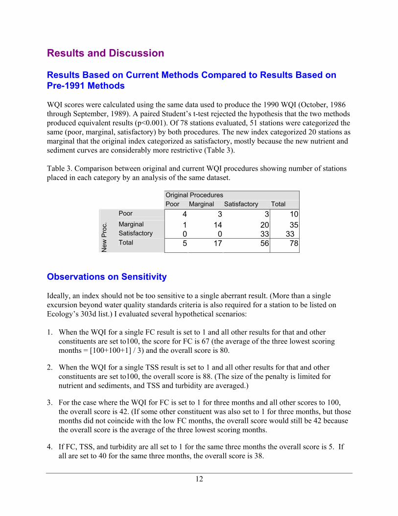
Results and Discussion Results Based on Current Methods Compared to Results Based on Pre-1991 Methods WQI scores were calculated using the same data used to produce the 1990 WQI (October, 1986 through September, 1989). A paired Student’s t-test rejected the hypothesis that the two methods produced equivalent results (p<0.001). Of 78 stations evaluated, 51 stations were categorized the same (poor, marginal, satisfactory) by both procedures. The new index categorized 20 stations as marginal that the original index categorized as satisfactory, mostly because the new nutrient and sediment curves are considerably more restrictive (Table 3). Table 3. Comparison between original and current WQI procedures showing number of stations placed in each category by an analysis of the same dataset.

Original Procedures Poor Marginal Satisfactory Total Poor 4 3 3 10 Marginal 1 14 20 35 Satisfactory 0 0 33 33

New

Pro

c.

Total 5 17 56 78

Observations on Sensitivity Ideally, an index should not be too sensitive to a single aberrant result. (More than a single excursion beyond water quality standards criteria is also required for a station to be listed on Ecology’s 303d list.) I evaluated several hypothetical scenarios: 1. When the WQI for a single FC result is set to 1 and all other results for that and other

constituents are set to100, the score for FC is 67 (the average of the three lowest scoring months = [100+100+1] / 3) and the overall score is 80.

2. When the WQI for a single TSS result is set to 1 and all other results for that and other constituents are set to100, the overall score is 88. (The size of the penalty is limited for nutrient and sediments, and TSS and turbidity are averaged.)

3. For the case where the WQI for FC is set to 1 for three months and all other scores to 100, the overall score is 42. (If some other constituent was also set to 1 for three months, but those months did not coincide with the low FC months, the overall score would still be 42 because the overall score is the average of the three lowest scoring months.

4. If FC, TSS, and turbidity are all set to 1 for the same three months the overall score is 5. If all are set to 40 for the same three months, the overall score is 38.

13

In summary, a single extremely poor result will still yield a good to moderate overall WQI score. Extremely poor results in three different months yield a moderate to poor overall index score. Two poor-scoring constituents during the same three months will result in a very low overall index score. Because the constituent score is an average of the three worst months (except for temperature, pH, and oxygen), it is possible to have two months where results violate the water quality criterion, yet have the constituent score indicate water quality met expectations ("low concern"). For example, two FC measurements of 230 colonies/100 mL in a Class A stream (equating to scores of 70) averaged with a score of 100 would yield an overall constituent score of 80. Trends A batch analysis of trends in monthly WQI scores (after aggregating individual constituents) was performed using WQHydro (Aroner, 2002). Trends were also performed on monthly scores adjusted for variability in flow, as described above. Reported probabilities include corrections for auto-correlation. Prior to adjusting for flow, statistically significant (p < 0.05) improving trends were indicated at four stations and declining trends at one station (table 4). Adjusting for flow increased the trend slope at nearly three quarters of the stations and resulted in improving trends at 9 stations and no declining trends. That is, trends in flow were apparently masking improving trends in water quality at most stations. Whether that is because flows were increasing or decreasing has not been evaluated and is station-specific, depending on which constituent(s) drive the WQI at a particular station. Some constituents are positively correlated with flow (e.g., sediment and nutrients) and some negatively (e.g., temperature and pH). Let’s examine a few stations and see what is happening. (Note: In the following discussion I report p-values as an indication of the potential contribution of trends in particular constituents towards trends in the monthly WQI scores. Although these trends are not statistically significant unless the probability is ≤ 0.05, the direction and consistency of the trend, significant or not, has bearing on the aggregated trend.) Puyallup River at Meridian Street (10A070) Monthly WQI scores improved significantly at this station (p=0.010). Sediment was the most frequent contributor to low scores, though nutrients and fecal coliform bacteria scores were also moderate. Trends in the raw data (not converted to WQI scores) for these constituents are shown in table 4.

14

Table 4. Trends in various constituents contributing to lower WQI scores at Puyallup River at Meridian Street (significance: *=80%, **=90%, ***=95%, ****=99%).

Constituent Slope (units/yr) Two-sided p value TSS (mg/L) -1.20a 0.20* Turb (NTN) +0.065a 0.58 TN (mg/L) -0.008b 0.09** TP (mg/L) +0.001a 0.23 FC (col./100mL) -9.55 0.007****

a Significant seasonality in trend results b Nitrogen was more likely than phosphorus to be the limiting nutrient In aggregate, the overall WQI identified improving conditions. This is a reasonable interpretation of the individual trend results, above. Palouse River at Palouse (34A170) This station exhibited an improving trend after adjusting for flow, but no trend at all prior to flow adjustment. Although almost all constituents produced low scores on occasion, turbidity typically had worse scores than other constituents. Raw turbidity measurements (prior to converting to WQI scores) increased, though not significantly at the 95% level (p=0.11). There was a significant increasing trend in flow, however (p=0.035) and, because turbidity was positively correlated with flow, adjusting the raw turbidity values for flow resulted in a decreasing adjusted-turbidity trend (p=0.017). In other words, had flow remained stable rather than increasing during the period, turbidity might have decreased. The effect of trends in flow on overall WQI scores can be complicated, however. While some constituents, like turbidity, get worse with increasing flow, others, like temperature, may get better. Furthermore, there may be differences between seasons and some WQI transformations have seasonal components. Methow River near Pateros (48A070) This was the only station that exhibited a significant worsening trend in overall WQI (slope=-0.18 units/year, p<0.05; Figure 4). (Still, quality was good at this station; overall annual scores were always in the “good” category and the flow-adjusted trend was not significant.) Annually, only pH, temperature, and sediment had more than a single result in the “moderate” category. Trends in the raw data, not converted to WQI scores, are shown in table 5.

15

Table 5. Trends in flow and constituents included in the WQI at Methow River near Pateros (significance: *=80%, **=90%, ***=95%, ****=99%).

Constituent Slope (units/yr) Two-sided p value FC (col./100mL) -0.0000a 0.60 Oxygen (mg/L) 0.0006b 0.78 TN (mg/L) -0.0033 0.52 TP (mg/L) +0.0000a 0.09** TSS (mg/L) +0.0000a 0.88 Turb NTU) 0.024 0.23 PH (std. units) 0.017b 0.10** Temp (C) -0.080b 0.34 Flow (cfs)c 30.7 0.07**

a A slope of zero can occur even if a trend is present when there are numerous identical results (e.g., multiple results below detection).

b There was significant seasonality in trend results c This analysis was based on instantaneous flow at the time of monthly sampling; trends in

continuous data may be different.

Figure 4. Monthly WQI scores at Methow River near Pateros with and without correction for

flow. Constituents contributing the most to some of the lower scores are shown.

16

There were no statistically significant (p < 0.05) worsening trends in the raw data and half the constituents had slopes indicative of improvement (though not significant). Why overall WQI scores have been declining is not entirely clear from table 5. pH contributed most to the declining trend (based on comparing the effect of removing each constituent from the aggregation and trend analysis); without pH, the trend was not significant, though the slope was still negative (slope=-0.06 units/year, p=0.14). It is difficult to identify a cause of the worsening trend in monthly WQI scores because no single constituent dominates the WQI aggregation. Sediment, pH, temperature, TP, and, to a lesser degree, FC all contribute at different times to produce the occasional moderate monthly WQI score (figure 4). Only in aggregation is there a declining trend. This may be an example of an aggregate trend reflecting subtle changes in water quality (related to flow since there was no flow-adjusted trend) not detectable by examining single constituents. I will not claim that water quality is deteriorating here without better support from the raw data, but this station warrants closer scrutiny. Nooksack River at Brennan (01A050) While the Methow at Pateros illustrates an overall WQI trend that is not entirely supported by the underlying data, the Nooksack at Brennan illustrates the opposite: the lack of a trend in its WQI scores even though trends in the underlying data are present. The trend in monthly WQI scores was not significant (0.63 units per year, p=0.42), yet FC counts decreased significantly (–4.7 colonies/100mL per year, p=0.012). In the Nooksack, clear improvements in fecal bacteria counts were masked by modest increases in sediment and nitrogen concentrations (Hallock, 2002). Trends in monthly WQI scores are, like the scores themselves, useful as a communication tool for non-technical purposes, and to help focus further data analysis efforts. One should use caution when interpreting scores, however, for several reasons: • Trends may be a result of changes in flow during the period being evaluated, and not due to

anthropogenic changes in the watershed (beside those that affect flow). Likewise, improving (or deteriorating) conditions in the watershed may be masked by changes in flow. Examining flow-adjusted trends can help explain this effect, but the relationship between flow, the WQI, and trends is complicated, in part because some WQI constituents have seasonal components.

• Trends may be hidden by the transformation process. Setting maximum and minimum WQI scores to 100 and (more rarely) to 1 censors some data sets. This may make it more difficult to detect trends in data sets with very low or very high values.

• The summarization process may hide trends in individual constituents; improvements (or deterioration) in particular water quality constituents may be overlooked.

• A significant trend in WQI scores may not be statistically supported by the underlying data. This could happen when there is apparent improvement (or deterioration) in several constituents that, individually, are not significant.

17

Literature Cited

Aroner, Eric, 2002. WQHydro: Water Quality-Hydrology Statistics/Graphics/Analysis Package. WQHydro Consulting, Portland, OR.

Brown, R. M., N. I. McClelland, R. A. Deininger, and R. G. Tozer. 1970. A Water Quality

Index—Do We Dare? Wat. Sewage Wks., 339-343. Couillard, D. and Y. Lefebvre, 1985. Analysis of Water Quality Indices. Journal of

Environmental Management 21:161-179. Cude, C. 2001. Oregon Water Quality Index: A Tool for Evaluating Water Quality Management

Effectiveness. Journal of the American Water Resources Association 37(1): 125-137. Hallock, D. 1990. Results of the 1990 Water Quality Index Analysis. Washington Department of

Ecology, Memorandum to Dick Cunningham, July 18, 1990. Washington Department of Ecology, Environmental Investigations and Laboratory Services Program, Olympia, WA.

Hallock, D. 2001. River and Stream Ambient Monitoring Report for Water Year 2000.

Washington Department of Ecology, Environmental Assessment Program, Olympia, WA. Publication No. 01-03-042, 14 pp. + appendices.

Hallock, D. 2002. Water Quality Assessment of the Nooksack River between Brennan and North

Cedarville. Washington Department of Ecology, Environmental Assessment Program, Olympia, WA. Publication No. 02-03-037, 22 pp. + appendices.

Harkins, R.D. 1974. An objective water quality index. J. Water Poll. Control Fed., 46(3):588-

591. McClelland, N.I., 1974. Water Quality Index Application in the Kansas River Basin, US

Environmental Protection Agency, Kansas City, MO, EPA-907/9-74-001. Omernik and Gallant, 1986. Ecoregions of the Pacific Northwest. US Environmental Protection

Agency, Environmental Research Laboratory, Corvallis, OR, EPA/600/3-86/003. Ott, W. R. 1978. Environmental Indices: Theory and Practice. Ann Arbor: Ann Arbor Science

Publishers, Inc. Peterson, R., 2001. Personal communication, March 1, 2001. Peterson, R. and B. Bogue. 1989. Water Quality Index (Used in Environmental Assessments),

EPA Region 10, Seattle WA.

18

Appendix A Coefficients of the quadratic equation WQI=a + b1 (Constituent) + b2 (Constituent)2 used to convert results to index scores. The particular formula used for a given station and constituent depends on the class (AA, A, or B), the Ecoregion, whether there are site-specific criteria (S in the “Class” column), and, sometimes, the season (“Low” = June through October, “High” = November through May except for some special curves) and result range. The “Log” column indicates whether the natural log of the constituent was used.

Constituent Class

or Ecorgn

Season Criterion Lower Result

Upper Result a b1 b2 Log

FC A All 100 0 999999 103.59 0.810055 -1.28485 Yes FC AA All 50 0 999999 103.25 -0.5832 -1.35641 Yes FC B All 200 0 999999 102.944 2.59723 -1.30612 Yes Oxygen A All 8 0 12 -67.3255 27.5473 -1.14663 Oxygen A All 8 12.001 99 100 0 0 Oxygen AA All 9.5 0 12.5 -131.2 33.81 -1.22397 Oxygen AA All 9.5 12.501 99 100 0 0 Oxygen B All 6.5 0 8.5 -109.509 43.6529 -2.23081 Oxygen B All 6.5 8.501 99 100 0 0 Oxygen S Low 5 0 7.5 -64.4444 42.7778 2.7778 Oxygen S Low 5 7.501 99 100 0 0 Oxygen S High 8 0 12 -62.3255 27.5473 -1.14663 Oxygen S High 8 12.001 99 100 0 0 Oxygen S2 All 5 0 7.5 -64.4444 42.7778 2.7778 Oxygen S2 All 5 7.501 99 100 0 0 pH A All 6.5 4 7.5 -531.422 158.619 -9.92672 pH A All 8.5 7.501 9.9 -338.912 128.627 -9.33089 ph AA All 6.5 4 7.5 -531.422 158.619 -9.92672 ph AA All 8.5 7.501 9.9 -338.912 128.627 -9.33089 pH B All 6.5 4 7.5 -531.422 158.619 -9.92672 pH B All 8.5 7.501 9.9 -338.912 128.627 -9.33089 TSS 1 High 0 0 999 100.7321 -5.17377 -1.31478 Yes TSS 1 Low 0 0 999 102.3444 -19.28875 0.087332 Yes TSS 2 High 0 0 999 100.7779 1.47273 -2.16014 Yes TSS 2 Low 0 0 999 109.9171 -11.2787 -0.698103 Yes TSS 4 High 0 0 999 100.9078 -7.1956 -2.26536 Yes TSS 4 Low 0 0 999 102.5005 -26.039 -0.768096 Yes TSS 7 High 0 0 999 101.1482 -4.23136 -1.33006 Yes

19

Constituent Class

or Ecorgn

Season Criterion Lower Result

Upper Result a b1 b2 Log

TSS 7 Low 0 0 999 100.2034 8.49706 -5.17937 Yes TSS 8 High 0 0 999 102.687 -17.5256 0.467769 Yes TSS 8 Low 0 0 999 101.9152 -17.2765 -1.39424 Yes Temp A All 18 -9 99 107.615 0.923907 -0.135563 Temp AA All 16 -9 99 100 0.923907 -0.135563 Temp B All 21 -9 99 88.1234 3.9808 -0.207885 Temp S All 20 -9 99 104.8229 2.00886 -0.162453 TP 1 High 0 0 999 -22.3043 -31.2067 -0.9088 Yes TP 1 Low 0 0 999 -45.6435 -22.4357 2.11808 Yes TP 2 High 0 0 999 -26.2561 -45.216 -3.80483 Yes TP 2 Low 0 0 999 -68.0023 -57.8648 -4.57211 Yes TP 4 High 0 0 999 -26.6586 -13.7327 3.09295 Yes TP 4 Low 0 0 999 -82.351 -38.6091 0 Yes TP 7 High 0 0 999 24.1568 -26.8113 -2.18636 Yes TP 7 Low 0 0 999 28.3779 -17.2759 -0.2800899 Yes TP 8 High 0 0 999 -57.6117 -58.0565 -5.11388 Yes TP 8 Low 0 0 999 -39.2805 -29.7187 0.2257024 Yes TN 1 High 0 0 999 102.3021 -43.1882 -19.7641 TN 1 Low 0 0 999 102.9609 -95.9463 0 TN 2 High 0 0 999 102.55 -3.86202 -61.1364 TN 2 Low 0 0 999 103.4779 -42.5636 -51.5611 TN 4 High 0 0 999 113.2895 -239.5035 0 TN 4 Low 0 0 999 109.63 -296.296 0 TN 7 High 0 0 999 100.9614 -15.1479 0.662255 TN 7 Low 0 0 999 100 -14.14 0 TN 8 High 0 0 999 100.3186 4.9998 -31.2691 TN 8 Low 0 0 999 100 10 -35 Turb 1 High 0 0 999 99.6621 -4.05247 -2.00526 Yes Turb 1 Low 0 0 999 92.3579 -14.1133 -1.1457 Yes Turb 2 High 0 0 999 101.1178 -0.037926 -2.61866 Yes Turb 2 Low 0 0 999 100.2948 -5.87364 -2.06283 Yes Turb 4 High 0 0 999 90.9645 -16.2966 -0.301131 Yes Turb 4 Low 0 0 999 83.9815 -26.125 0.61845 Yes Turb 7 High 0 0 999 99.1624 -6.43442 -1.31263 Yes Turb 7 Low 0 0 999 99.6197 -4.43165 -3.1984 Yes Turb 8 High 0 0 999 96.1118 -18.16 0.48295 Yes Turb 8 Low 0 0 999 93.4405 -23.2416 -1.71641 Yes

20

Appendix B Distribution of nutrient and sediment constituents at long-term stations from October 1990 through September 2001. (Flow season: Low-June through October, High-November through May).

Water Quality Index: 100 80 40 20

TSS (mg/L) High-Flow Season Ecorgn N 1% 5% 10% 20% 50% 80% 90% 95% 99%

Coast 356 1 1 1 2 4 15 50 131 497 Non-Gla 246 1 1 1 2 4 15 58 188 503 Glacial 110 1 1 2 2 6 19 48 92 581 Puget 1675 1 2 2 4 12 45 96 206 723 Non-Gla 1232 1 1 2 3 9 32 77 140 595 Glacial 443 3 5 6 8 23 84 204 385 1282 Cascades 272 1 1 1 1 2 8 16 37 108 Non-Gla 195 1 1 1 1 3 9 19 42 183 Glacial 77 1 1 1 1 1 4 11 19 88 Columbia 1469 1 1 1 2 6 27 66 127 690 Rockies 339 1 1 1 2 3 8 15 26 323

TSS (mg/L) Low-Flow Season ECORGN N 1% 5% 10% 20% 50% 80% 90% 95% 99%

Coast 259 1 1 1 1 2 5 7 17 88 Non-Gla 179 1 1 1 1 2 4 5 16 100 Glacial 80 1 1 1 2 3 6 12 28 95 Puget 1192 1 1 2 2 5 16 35 78 397 Non-Gla 877 1 1 1 2 4 8 13 25 137 Glacial 315 3 4 5 7 17 59 105 168 487 Cascades 190 1 1 1 1 2 4 6 8 38 Non-Gla 136 1 1 1 1 3 5 6 9 71 Glacial 54 1 1 1 1 2 4 6 8 32 Columbia 1083 1 1 1 2 6 21 40 68 133 Rockies 250 1 1 1 1 2 5 8 12 43

TURB (NTU) High-Flow Season ECORGN N 1% 5% 10% 20% 50% 80% 90% 95% 99%

Coast 357 0.5 0.6 0.8 1.3 3.1 11.4 33.6 80.0 231.0 Non-Gla 245 0.4 0.5 0.7 1.0 2.4 9.7 29.4 87.0 281.6 Glacial 112 0.9 1.0 1.3 2.0 5.5 16.6 45.0 80.0 192.9 Puget 1667 0.5 1.0 1.4 2.2 6.3 24.0 50.0 90.0 290.0 Non-Gla 1225 0.5 0.8 1.2 1.8 5.3 20.0 40.0 73.5 274.8 Glacial 442 1.7 2.1 2.7 3.9 10.5 34.0 75.0 140.0 623.7 Cascades 272 0.2 0.5 0.5 0.6 1.3 3.1 7.0 12.3 65.4 Non-Gla 195 0.2 0.5 0.6 0.8 1.6 4.4 9.0 14.6 91.2 Glacial 77 0.2 0.3 0.5 0.5 0.9 1.8 2.5 4.0 28.0 Columbia 1468 0.4 0.5 0.7 1.1 3.9 16.0 34.0 60.0 346.2 Rockies 338 0.4 0.5 0.7 0.9 1.7 4.7 7.7 15.2 141.7

21

Turb (NTU) Low-Flow Season ECORGN N 1% 5% 10% 20% 50% 80% 90% 95% 99%

Coast 259 0.3 0.5 0.5 0.6 1.4 3.3 7.4 14.0 55.0 Non-Gla 179 0.3 0.5 0.5 0.6 1.0 2.0 2.8 5.8 57.0 Glacial 80 0.5 0.5 0.7 0.9 3.2 9.4 13.0 18.0 55.0 Puget 1206 0.5 0.7 0.9 1.2 2.5 10.0 24.0 49.6 160.0 Non-Gla 888 0.5 0.6 0.8 1.0 1.8 4.1 8.1 17.0 91.7 Glacial 318 1.5 1.9 2.4 3.4 11.0 37.2 60.0 95.3 232.4 Cascades 189 0.3 0.5 0.5 0.6 1.1 1.9 2.5 3.5 14.9 Non-Gla 135 0.2 0.5 0.5 0.5 1.0 1.7 2.4 3.3 36.0 Glacial 54 0.5 0.6 0.7 0.8 1.4 2.3 3.1 3.8 9.2 Columbia 1082 0.4 0.5 0.7 1.0 2.6 8.8 18.0 30.0 85.0 Rockies 250 0.5 0.6 0.7 0.8 1.2 2.1 3.2 6.2 15.0

TP (mg/L) High-flow Season ECORN N 1% 5% 10% 20% 50% 80% 90% 95% 99%

Coast 358 0.010 0.010 0.010 0.010 0.017 0.037 0.060 0.083 0.266 Puget 1677 0.010 0.010 0.010 0.014 0.028 0.055 0.085 0.135 0.352 Cascades 269 0.009 0.010 0.010 0.010 0.011 0.020 0.031 0.046 0.111 Columbia 1450 0.010 0.010 0.010 0.013 0.041 0.117 0.192 0.341 1.315 Rockies 335 0.010 0.010 0.010 0.010 0.021 0.049 0.071 0.094 0.230

TP (mg/L) Low-flow Season ECORN N 1% 5% 10% 20% 50% 80% 90% 95% 99%


TN (mg/L) High-flow Season ECORN N 1% 5% 10% 20% 50% 80% 90% 95% 99%


TN (mg/L) Low-Flow Season ECORN N 1% 5% 10% 20% 50% 80% 90% 95% 99%


22

Appendix C Trends in monthly WQI scores at long-term stations. Positive slopes indicate improving conditions. P=probability. Statistical significance (“Sign.”): 80% (*), 90% (**), 95% (***), and 99% (****). Not Flow-adjusted Adjusted for Flow Station STANAME Slope p Sign. Slope p Sign. 01A050 Nooksack R. @ Brennan 0.6255 0.4243 1.1787 0.1155 * 01A120 Nooksack R @ No Cedarville 0.3289 0.3172 0.6397 0.3353 03A060 Skagit R nr Mount Vernon 0.1595 0.1076 * 0.4365 0.0873 ** 03B050 Samish R nr Burlington 0.7984 0.1647 * 0.3761 0.4271 04A100 Skagit R @ Marblemount 0.1216 0.6883 0.2191 0.2009 05A070 Stillaguamish R nr Silvana 0.1048 0.8098 1.0394 0.0289 *** 05A090 SF Stillaguamish @ Arlington -0.1231 0.6252 4.4290 0.2131 05A110 SF Stilly nr Granite Falls 0.2290 0.3421 05B070 NF Stillaguamish @ Cicero 0.4066 0.1886 * 0.8345 0.1640 *

05B110 NF Stillaguamish nr Darrington -0.4803 0.6579 -0.1144 0.8770

07A090 Snohomish R @ Snohomish 0.2591 0.0363 *** 0.4428 0.0071 **** 07C070 Skykomish R @ Monroe 0.1590 0.0679 ** 0.2560 0.0116 *** 07D050 Snoqualmie R nr Monroe 0.3633 0.2805 0.7795 0.0652 ** 07D130 Snoqualmie R @ Snoqualmie 0.1173 0.0916 ** 0.0962 0.4392 08C070 Cedar R @ Logan St/Renton -0.0421 0.7558 -0.0197 0.8297 08C110 Cedar R nr Landsburg 0.0673 0.2725 0.0156 0.6137 09A080 Green R @ Tukwila 0.9447 0.0836 ** 0.8805 0.1096 * 09A190 Green R @ Kanaskat 0.1030 0.1550 * 0.0872 0.1220 * 10A070 Puyallup R @ Meridian St 1.4928 0.0102 *** 1.7195 0.0112 *** 11A070 Nisqually R @ Nisqually 0.0425 0.7276 0.6388 0.0267 *** 13A060 Deschutes R @ E St Bridge -0.8074 0.2589 -0.7721 0.0870 ** 16A070 Skokomish R nr Potlatch 0.2208 0.0478 *** 0.2873 0.0095 **** 16C090 Duckabush R nr Brinnon 0.0216 0.7585 0.0628 0.4817 18B070 Elwha R nr Port Angeles 0.1260 0.2181 0.1537 0.1077 * 20B070 Hoh R @ DNR Campground 0.0067 0.9705 0.3461 0.1092 * 22A070 Humptulips R nr Humptulips 0.0720 0.4929 0.5351 0.0168 *** 23A070 Chehalis R @ Porter -0.3493 0.4203 -0.6246 0.0879 ** 23A160 Chehalis R @ Dryad -0.0582 0.5866 0.2385 0.3648 24B090 Willapa R nr Willapa 0.7374 0.3083 0.3380 0.4836 24F070 Naselle R nr Naselle 0.0464 0.8695 0.3000 0.3168 26B070 Cowlitz R @ Kelso -0.1572 0.7592 0.6765 0.1732 * 27B070 Kalama R nr Kalama 0.0213 0.9759 -0.8470 0.2202 27D090 EF Lewis R nr Dollar Corner -0.0866 0.2379 -0.0263 0.6109 31A070 Columbia R @ Umatilla 0.0920 0.5548 0.1019 0.4820 32A070 Walla Walla R nr Touchet 1.5411 0.0516 ** 1.6406 0.0163 *** 33A050 Snake R nr Pasco 0.2976 0.1792 * 0.3373 0.3034 34A070 Palouse R @ Hooper 0.0389 0.9552 0.1454 0.7486

23

Not Flow-adjusted Adjusted for Flow Station STANAME Slope p Sign. Slope p Sign. 34A170 Palouse R @ Palouse 0.1369 0.6192 0.7530 0.0331 *** 34B110 SF Palouse R @ Pullman 1.6408 0.0178 *** 1.4500 0.0681 ** 35A150 Snake R @ Interstate Br -0.1401 0.4771 -0.0038 0.9361 35B060 Tucannon R @ Powers 1.4140 0.1098 * 1.1226 0.1329 * 36A070 Columbia R nr Vernita 0.1690 0.3276 0.1771 0.3353 37A090 Yakima R @ Kiona 0.0324 0.9408 0.9192 0.1822 * 37A205 Yakima R @ Nob Hill 0.2708 0.3649 -0.6141 0.1469 * 39A090 Yakima R nr Cle Elum 0.0504 0.7652 -0.0920 0.7457 41A070 Crab Cr nr Beverly -0.2443 0.6160 -0.3141 0.3822 45A070 Wenatchee R @ Wenatchee -0.2428 0.1185 * -0.2744 0.1437 * 45A110 Wenatchee R nr Leavenworth -0.0367 0.7987 0.0859 0.5040 46A070 Entiat R nr Entiat -0.0060 0.9110 0.0617 0.1696 * 48A070 Methow R nr Pateros -0.1824 0.0151 *** -0.0736 0.2728 48A140 Methow R @ Twisp -0.0413 0.1915 * -0.0241 0.7618 49A070 Okanogan R @ Malott 0.0438 0.7836 0.2049 0.1175 * 49A190 Okanogan R @ Oroville 0.0765 0.7713 0.1537 0.4425 49B070 Similkameen R @ Oroville 0.0371 0.8192 0.0491 0.7333 53A070 Columbia R @ Grand Coulee 0.0781 0.1916 * 0.0645 0.2367 54A120 Spokane R @ Riverside SP -0.3766 0.4001 0.5544 0.0728 ** 55B070 Little Spokane R nr Mouth -1.9217 0.0633 ** -0.8903 0.0635 ** 56A070 Hangman Cr @ Mouth 0.2946 0.7460 0.0060 1.0000 57A150 Spokane R @ Stateline Br 0.0290 0.6291 -0.0744 0.3734 60A070 Kettle R nr Barstow 0.0948 0.7690 0.1198 0.5956 61A070 Columbia R @ Northport 0.1230 0.3502 0.3258 0.0777 ** 62A150 Pend Oreille R @ Newport -0.0236 0.8549 0.0854 0.7763

Documents

A Water Quality Index for Ecology's Stream Monitoring Program