A WALL INTERFERENCE

ASSESSMENT/CORRECTION

SYSTEM

SEMI-ANNUAL

REPORT #1

Dr. C.F. Lo, Principal Investigator

University of Tennessee Space Institute

Covering the period June 1991 through December 1991

Under NASA Ames Research Center NAG 2-733

Ames Research Center

Moffett Field, CA 94035-1000

INSTITUTION:

CSTAR - Center for Space

Transportation and Applied Research

UTSI Research Park

Tullahoma, TN 37388-8897

Phone 615-455-9294 or 5884

https://ntrs.nasa.gov/search.jsp?R=19920006756 2018-09-09T11:35:51+00:00Z

Title: A Wall Interference Assessrnent/Correction System

Semi-Annual ReportJune - December, 1991

"-,r-

Principal Investigator:Dr. C. F. Lo, UTSI

Other Investigators:Dr. J. C. Erickson, CSTARMr. N. Ulbrich, GRA/UTSI

Technical Officer:Dr. Frank W. Steinle, NASA/Ames Research Center

Technical Objectives

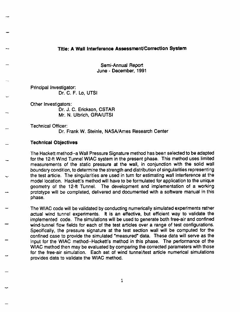
The Hackett method--a Wall Pressure Signature method has been selected to be adapted

for the 12-ft Wind Tunnel WlAC system in the present phase. This method uses limitedmeasurements of the static pressure at the wall, in conjunction with the solid wall

boundary condition, to determine the strength and distribution of singularities representingthe test article. The singularities are used in turn for estimating wall interference at themodel location. Hackett's method will have to be formulated for application to the unique

geometry of the 12-ft Tunnel. The development and implementation of a workingprototype will be completed, delivered and documented with a software manual in thisphase.

The WIAC code will be validated by conducting numerically simulated experiments ratheractual wind tunnel experiments. It is an effective, but efficient way to validate the

implemented code. The simulations will be used to generate both free-air and confinedwind-tunnel flow fields for each of the test articles over a range of test configurations.Specifically, the pressure signature at the test section wall will be computed for theconfined case to provide the simulated "measured" data. These data will serve as theinput for the WlAC method--Hackett's method in this phase. The performance of theWlAC method then may be evaluated by comparing the corrected parameters with thosefor the free-air simulation. Each set of wind tunnel/test article numerical simulations

provides data to validate the WlAC method.

Status of Progress

1. System Validation Design

A numerical wind tunnel test simulation is planned to be utilized to validate the WIACmethods developed in the project, specifically to the wall pressure signature method--Hackett's method in the current phase. A low-order potential-flow panel method has beenselected to simulate the wind tunnel and test article geometries for its flexibility.

A copy of the low-order panel code, called PMARC (Panel Method Ames ResearchCenter), was obtained from Dr. Frank Steinle, technical monitor. The code of PMARC(Ref. 1) is a well-documented code with open architecture which has several advancedfeatures including internal flow modeling for wind tunnel application. The code hasanother feature allowing the adjustment of the size of panel for suiting the computerhardware and the size of the problem. PMARC can be run on computers ranging froma Macintosh II workstation to a Cray Y-MP.

Currently, the copy of PMARC (version 12) has been compiled on a IBM R6000 andchecked out on two sample cases -- wing and wing/body which have been provided byNASA/ARC. The PMAPP, a post processor for PMARC, will be received fromNASA/ARC shortly.

2. Hackett's Method Implementation

The implementation of a Wall Pressure Signature method which is based upon the wallinterference method developed by Hackett (Ref. 2) has been initiated. In the presentreported period, the blockage correction is developed and implemented. The liftingcorrection will be carried out in the next period. A working computer code has beenimplemented and verified by an analytic solution.

The analytic flow field solution of a rectangular wind tunnel with a finite airfoil wing andits wake was derived as a bench mark solution to verify the solution calculated byHackett's Method. The blockage correction of the Wall Pressure Signature method

(Hackett's Method) for this wing/wake case is obtained and verified by the analyticalsolution.

The detailed development and results are given in Attachment I.

Future Plan

1. Panel Code Application

2

The application of panel code PMARC will be initiated for Ames 12-ft Wind Tunnel. Thewall pressure in using Hackett's method will be computed for the cases of wing andwing/body configuration. The post processor (PMAPP) for PMARC will be installed onthe UTSI's computer to support PMARC's application. The software system validationwill be started for Hackett's method developed in Task 2 with the configuration of 12-ftTunnel.

2. Lifting Correction of Hackett's Method

The development and implementation of the lifting Correction of Hackett's Method will beinitiated. The verification will be based on an independent solution such as acorresponding solution of lifting case derived in this reported period for the blockage case.

References

1. Ashby, D.L. et al, "Potential Flow Theory and Operation Guide for the Panel CodePMARC," NASA Tech. Memo 102851, January 1991

2. Hackett, J. E. et al, "A Review of the Wall Pressure Signature and other TunnelConstraint Correction Methods for High Angle-of-Attacks Tests", AGARD Report No. 692,May 1980

Attachment I

NASA Ames Research Center NAG 2-733

BLOCKAGE CORRECTION IN 3-DIMENSIONAL WIND TUNNEL

TESTING BASED ON THE WALL SIGNATURE METHOD

4

BLOCKAGE CORRECTION IN 3-DIMENSIONAL WIND TUNNEL

TESTING BASED ON THE WALL SIGNATURE METHOD

N. Ulbrich and C. F. Lo

The University of Tennessee Space Institute

Tullahoma, Tennessee 37388

Summary

A blockage correction technique in 3-dimensional wind tunnel flow fields is developed

and verified. Blockage corrections are obtained by Hackett's method with pressure mea-

surements on the wind tunnel wall.

An analytic wind tunnel flow field solution of a rectangular wing with parabolic airfoil

section and a trailing edge wake is presented. This analytic solution is used to simulate

pressure measurements on selected wall locations and to calculate the exact solution of the

blockage problem.

A pressure coefficent correction due to model blockage is obtained by Hackett's method

in using simulated wall pressure measurements. Pressure coefficient corrections show good

agreement with the exact solution of the blockage correction problem. This verifies the

implementation of Hackett's method for the blockage correction.

1. Introduction

The Wall Pressure Signature Technique (Hackett's method) _'2'3'4'5 is considered to

calculate blockage correction due to wall interference in the NASA/ARC 12ft Pressure

Wind Tunnel. The first part of this report presents the development and implementation

of an analytical correction technique which requires the simulation of wall pressure mea-

surements for Hackett's method. A wind tunnel with rectangular cross section is selected.

A rectangular wing with parabolic airfoil section is chosen as a test article and a solution

of this flow field is obtained by applying thin wing theory. The influence of the wake is

modeled by using a line source and a line sink. The analytic solution of the wind tunnel

flow field of a wing and a wake is obtained by combining free-air solutions with the method

of images.

Two important sets of data are derived from the analytic solution: wall pressure mea-

surements are simulated which will be used as required by Hackett's method to calculate

blockage corrections; the exact solution of the blockage problem is calculated to verify

Hackett's method. Basic steps of the development and verification of a blockage correction

technique based on wall pressure measurements are shown in Fig. 1.

A detailed description of Hackett's method is presented in the second part of this

report. It is shown how an equivalent flow field representation is defined based on wall

pressure measurements. This equivalent flow field model is then used in combination

with the method of images to calculate a blockage correction. This blockage correction is

compared to the exact solution of the blockage problem to verify Hackett's method.

-1-

2. Analytic Wind Tunnel Flow Field

2.1 General Remarks

The simulation of a three dimensional wind tunnel flow field requires the mathemati-

cal description of a simplified test article and a wake. A rectangular wing with parabolic

airfoil section is selected as a test article. In general the analytic solution of a wing in in-

compressible three-dimensional flow cannot be obtained easily. Integration of complicated

algebraic expressions is necessary.

The solution of the thickness problem of a thin wing in incompressible free-air flow is

known in the form of a double integral. Basic equations will be presented and the geometry

of the selected rectangular tunnel and wing will be specified. The free air solution is

obtained by direct integration. A wake in free-air flow can be simulated by using a finite

span line source and line sink. An analytic flow field solution will be derived by direct

integration as well.

The wind tunnel flow field will be calculated by superimposing the analytic solutions

of wing and wake and applying the method of images to the total flow field to satisfy the

wall boundary conditions.

Finally formulae of the analytic solution of the blockage problem are obtained.

2.2 Free-Air Flow Field of the Wing

The solution of the perturbation potential of three-dimensionai planar wings in in-

compressible free-air flow is given by Ashley and Landahl 6 as follows

r // Og(xl,yl) dxl dyl )_ z 2 (1) l(x,y,z) = - A (z-xl)2+(y-yl +

where 'A' is the projected wing area, 'r' is the thickness and Og(xl, y_)/c3xl is the thickness

slope.

Figure 2 shows a rectangular wing with parabolic airfoil section, wing span 's' and

chord length 'c'. The thickness function g(xl,yl) of the parabolic airfoil section has the

following form

: (2a)

The thickness slope is then given as

Og(xl,yl) Og(xl) = 2. [1 2xlOzl Ozl [ c

Combining Eqs.(1), (25) and knowing that 0 < x_ < c and -s/2 < y_ < s/2 we get

(2b)

¢ s/2

_,,(x,y,z) : - r_ . / / [1-2x,/c] dx, dyl

o -,Is

(3)

-2-

The dimensionlessaxial perturbation velocity is given as

or in terms of the correspondingpressurecoefficient

cp,(x,y,z) = - 2.ul(x, ,z) (5)

The integration of Eq.(4) is complicated. Different types of integrals have to be

considered depending on the choice of field point.

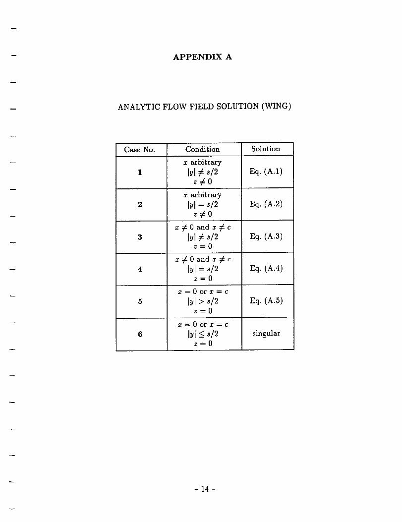
In general the solution consists of six cases to cover the entire flow field. The classi-

fication of these cases and the solution of the incompressible axial perturbation velocity

are given in Appendix A. Singularities exist at the leading and trailing edge of the wing.Otherwise a well defined solution can be found in the flow field.

A verification of parts of the solution is possible if the limit as the wing span goes to

infinity is taken. The axial perturbation velocity on the model surface is obtained based

on Eq. (A.3) and limits given in Appendix B. We get

limu(z,y,O) 4 ( 1 )= -.r. 1 + • [1 - 2xlc].ln Ixt¢l• ,, II-x/ l (6)

Equation (6) agrees with the solution of a two-dimensional parabolic airfoil section given

by Schlichting and Truckenbrodt 7.

Pressure coefficients in free-air on selected locations are calculated based on Eq. (5)

and the analytic solution given in the Appendix A. The following wing geometry is chosen:

chord length c = 1.0, wing span s = 4.0, thickness r = 0.1. Pressure coefficients are

calculated on the planes z = 0.0, 0.2. Results are presented in Figs. (3a) and (3b).

Singularities on the leading and trailing edge of the wing can be noticed in Fig. (3a). It

is obvious that the pressure coefficient distribution is symmetric with respect to the planes

y = 0.0 and x = c/2. This symmetry property can be used to reduce calculation time if

pressure coefficients in a plane with constant z-coordinate are determined. The absolute

value of the pressure coefficient decreases with inceasing z-coordinate as the perturbations

of the free-air flow field decay with increasing distance from the wing plane.

2.3 Free-Air Flow Field of the Trailing Edge Wake

The flow field of the trailing edge wake of a rectangular wing is simulated using a line

source located on the trailing edge and a line sink of equal strength at a large distance 'cs'

downstream of the trailing edge. The geometry of the wake model is given in Fig. (4).

The general solution of the velocity potential of a single line source of span 'bw' and

constant source strength 'q' in free-air flow is given by Katz and Plotkin s as

3

12

q f dl (7,0_(x,y,z) = -_. _/(x__,)2+(y__,)2+(__z,)_I1

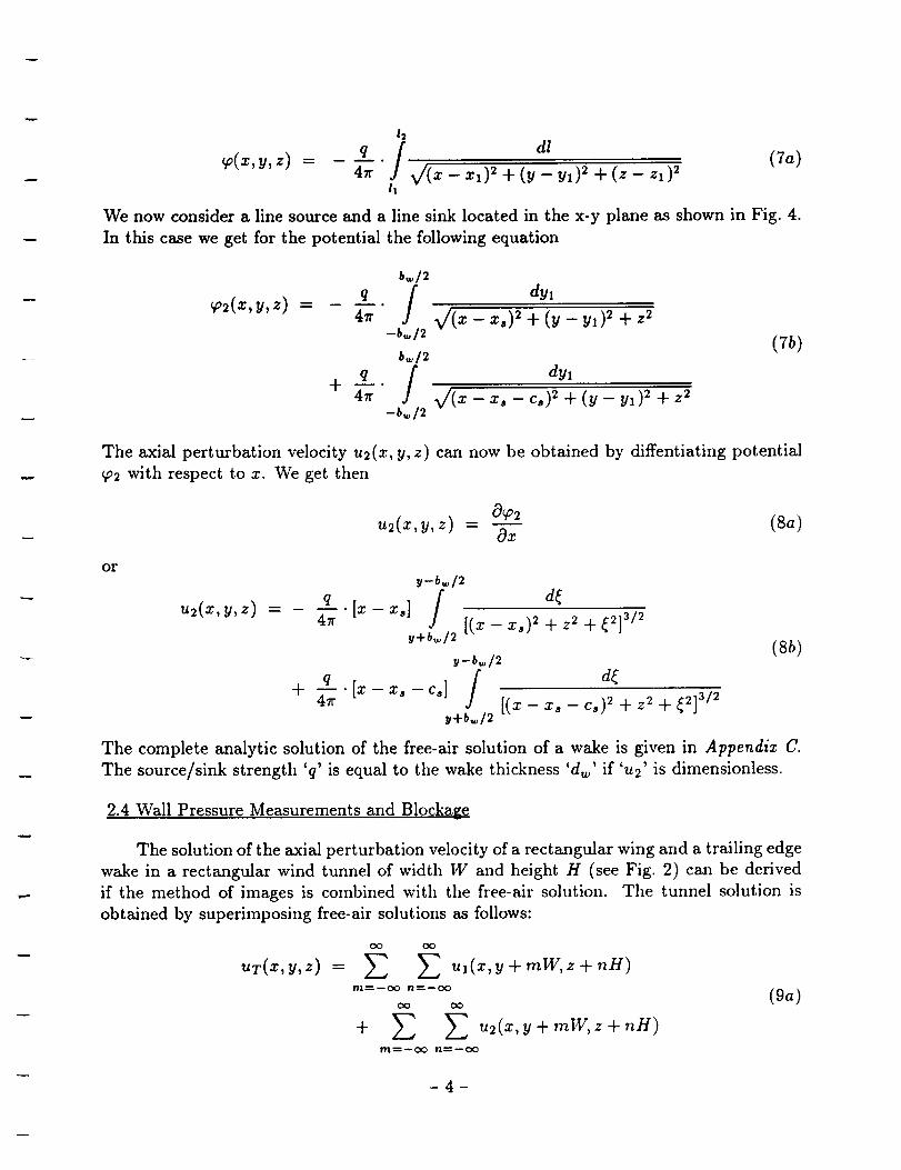
We now consider a line source and a line sink located in the x-y plane as shown in Fig. 4.

In this case we get for the potential the following equation

_2(x,y,z) =

b_/2

-b,,, /2

b,_12

,__./+ 47r

-b,o /2

dyl

_(_ - _,)_ + (_ - _,)_ + z_

dy_

(7b)

The axial perturbation velocity u2(x, y, z) can now be obtained by diffentiating potential

_2 with respect to x. We get then

u2(_,_,z)- a_2 (8a)Oz

ory-b_/2

P

d(q•[_- _,] /u2(x,y,z)

[(x - _,)_+ z_ + _]_/_y+b,,, /2

y-bvo /2P

d(q• [_-,.,-_,] /+

[(_ - _, - _,)_+ z_+ _]_/_,t/

_+b,./2

(Sb)

The complete analytic solution of the free-air solution of a wake is given in Appendiz C.

The source/sink strength 'q' is equal to the wake thickness 'dw' if 'u2' is dimensionless.

2.4 Wall Pressure Measurements and Blockage

The solution of the axial perturbation velocity of a rectangular wing and a trailing edge

wake in a rectangular wind tunnel of width W and height H (see Fig. 2) can be derived

if the method of images is combined with the free-air solution. The tunnel solution is

obtained by superimposing free-air solutions as follows:

OO OO

_ u,(x,y + mW, z + nil)Irirl_--O0 !111_00

O0 O0

+ _ )--_ u2(x,y+mW, z+nH)rtl_--O0 n_OD

(9a)

-4-

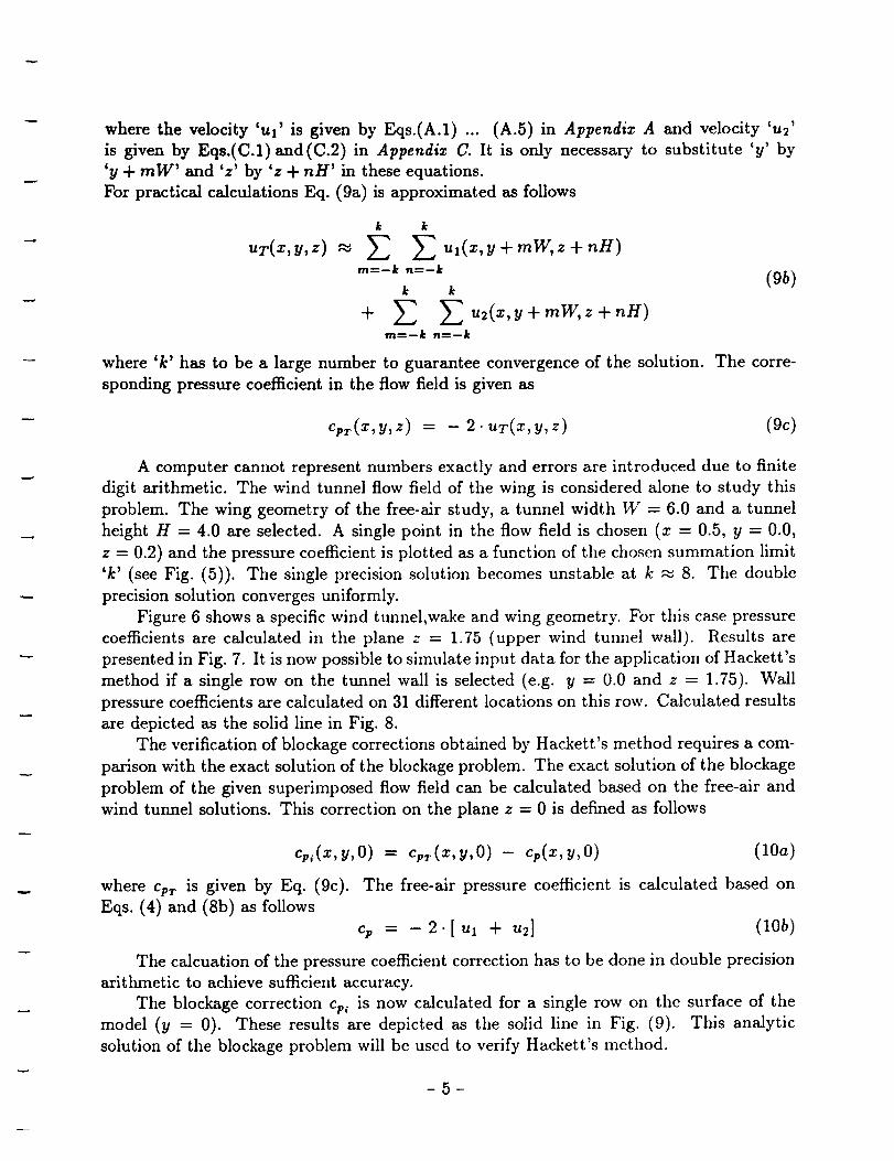
where the velocity 'UI' is given by Eqs.(A.1) ... (A.5) in Appendix A and velocity 'u2'

is given by Eqs.(C.1)and(C.2) in Appendix C. It is only necessary to substitute 'y' by

'y + roW' and 'z' by 'z + nil' in these equations.

For practical calculations Eq. (9a) is approximated as follows

k k

m=-k n=-k

k k

+ Z Z u2(x,y+mW, z+nH)

m-_--k n-_-k

where 'k' has to be a large number to guarantee convergence of the solution.

sponding pressure coefficient in the flow field is given as

(9b)

The corre-

%r(X,y,z) = -- 2. UT(X,y,z) (9c)

A computer cannot represent numbers exactly and errors are introduced due to finite

digit arithmetic. The wind tunnel flow field of the wing is considered alone to study this

problem. The wing geometry of the free-air study, a tunnel width W = 6.0 and a tunnel

height H = 4.0 are selected. A single point in the flow field is chosen (x = 0.5, y = 0.0,

z = 0.2) and the pressure coefficient is plotted as a function of the chosen summation limit

'k' (see Fig. (5)). The single precision solution becomes unstable at k _ 8. The double

precision solution converges uniformly.

Figure 6 shows a specific wind tunnel,wake and wing geometry. For this case pressure

coefficients are calculated in the plane z = 1.75 (upper wind tunnel wall). Results are

presented in Fig. 7. It is now possible to simulate input data for the application of Hackett's

method if a single row on the tunnel wall is selected (e.g. y = 0.0 and z = 1.75). Wall

pressure coefficients are calculated on 31 different locations on this row. Calculated results

are depicted as the solid line in Fig. 8.

The verification of blockage corrections obtained by Hackett's method requires a com-

parison with the exact solution of the blockage problem. The exact solution of the blockage

problem of the given superimposed flow field can be calculated based on the free-air and

wind tunnel solutions. This correction on the plane z = 0 is defined as follows

= - (10a)

where %r is given by Eq. (9c).

Eqs. (4) and (8b) as foUowsThe free-air pressure coefficient is calculated based on

cp = -2.[ + (10b)

The calcuation of the pressure coefficient correction has to be done in double precision

arithmetic to achieve sufficient accuracy.

The blockage correction cp_ is now calculated for a single row on the surface of the

model (y = 0). These results are depicted as the solid line in Fig. (9). This analytic

solution of the blockage problem will be used to verify Hackett's method.

-5-

;_. Hackett's Method

_.1 General Remarks

Wail pressure signature methods like Hackett's method were successfully applied in

the past to calculate blockage corrections in 3-dimensional wind tunnel testing. Hackett's

method consists of two major parts: the signature analysis of the wall pressure mea-

surements to model test articles and the calculation of blockage corrections based on the

simplified test article representation obtained from the signature analysis.

At first a description of the signature analysis will be presented. The signature analysis

is applied to a simulated wall signature which is calculated for a given wing, wake and wind

tunnel geometry as shown in Fig. 6. Secondly the simplified model/wake representation

is derived. Finally, blockage corrections are calculated based on the simplified model

representation and the method of images which are compared to the exact solution of the

blockage problem.

3.2 Signature Analysis

These simulated measurements of a selected model/wake/wind tunnel geometry are

obtained from the analytic solution described in Section 2.4 . Simulated wall pressure

coefficients on a selected wind tunnel wall (i.e. -2.5 < y < 2.5 and z = 1.75) are given in

Fig. 7. The signature analysis suggested by Hackett 2 is applied to simulated wall pressure

measurements on a single row (in our case y = 0.0 and z = 1.75; see Fig. 6).

The wall pressure measurement on the selected row (solid line in Fig. 8) is split into

a symmetric and antisymmetric part by iteration. This iteration requires that the peak

location of the symmetric signal is identical with the location of the inflection point of the

antisymmetric signal.

The symmetric part of the signal is related to a simplified representation of the solid

body blockage in the form of a line source/sink pair. The source/sink spacing and location

and the source sink strength can be determined from the width at half height of the

symmetric signal, the location of the velocity peak and the maximum value of the velocity.

The antisymmetric part is similarly related to a simplified representation of the wake.

Characteristic parameters (like line source/sink location and source/sink strength) are de-

rived from the location of the inflection point of the antisymmetric signal and the asymp-

totic value of the velocity far downstream of the model. More details on the signature

analysis are given by Hackett 2. A concise description of the method is also given by

Allmaras s.

3.3 Blockage (_orrection

Blockage corrections are now calculated based on the simplified test article and wake

representation which is given in terms of 4 line sources/sinks. The equations of the blockage

correction of the simplified test article and wake representation can be derived easily by

modifying equations presented in Appendix C and using the method of images. The result

of this calculation is given by the dashed line in Fig. 9 and compares well to the known

-6-

analytic solution of the blockage problem. Pressure coefficient corrections given in Fig. 9

have to be combined with wind tunnel measurements on the same location in the x-y-z

coordinate system to obtain the free-air measurements.

4. Remarks

Blockage corrections in a 3-dimensional wind tunnel flow field are calculated applying

Hackett's method to simulated wall pressure measurements. These corrections show excel-

lent agreement with the known analytic solution of the blockage problem. The influence

of a fuselage on the applicability of Hackett's method still has to be included in these pre-

limlnary results. An improvement of the signature analysis is also considered to simplify

the calculation of the equivalent test article and wake representation.

References

1Hackett, J. E., Wilsden, D. J., "Determination of Low Speed Wake Blockage Corrections

via Tunnel Wall Static Pressure Measurements", AGARD CP-174, October 1975.

2Hackett, J. E., Wilsden, D. J. and Lilley, D. E., "Estimation of Tunnel Blockage from

Wall Pressure Signatures: A Review and Data Correlation", NASA CR-152241, March

1979.

3Hackett, J. E., Wilsden, D. J. and Stevens, W. A., "A Review of the Wall Pressure Sig-

nature and other Tunnel Constraint Correction Methods for High Angle-of-Attack Tests",

AGARD Report No.692, May 1980.

4Hackett, J. E., "Living with Solid-Walled Wind Tunnels", AIAA-82-0583, presented at the

AIAA 12th Aerodynamic Testing Conference, March 22-24, 1919882/Williamsburg, Virginia.

5Allmaras, S. R., "On Blockage Corrections for Two-Dimensional Wind Tunnel Tests using

the Wall Pressure Signature Method", NASA-TM-86759, March 1986.

SAshley, H. and Landahl, M., "Aerodynamics of Wings and Bodies", Addison-Wesley

Publishing Company, Reading Massachusetts, p.129, Eq.(7-14).

7Schlichting, H. and Truckenbrodt, E., "Aerodynamics of the Airplane", translated by

H. J. Ramm, McGraw-HiU Intl. Book Company, p.71, Eq.(2-97).

SKatz, J. and Plotkin, A., "Low-Speed Aerodynamics - From Wing Theory to Panel Meth-

ods", McGraw-Hill Intl. Book Company, 1991, p.60, Eq.(3.26).

BLOCKAGE EFFECT

ANALYTICAL MODEL OF THE

WIND TUNNEL FLOW FIELD

... WING AND WAKE IWALL MEASUREMENT

...Iv I

VERIFICATION

HACKETT'S METHOD IWALL INTERFERENCE

... EQUIVALENT BODY

Fig. 1 Development and Verification of a 3-Dimensional

Blockage Correction Technique

-8-

Y

2X

Y \

Fig. 2 Wing and Wind Tunnel Geometry

"0

. :_sou

n _, -i1

Fig. 3a Pressure Coefficient (Free-Air Case, z = 0.0)

9

.O.4 ....!

.0.3...... .......

'"I _.

"0 .J"

U _"rt

o_ _ _._I_ _ ]..'" T'_

._o.'"I _ ........

I ---. _ --0.4

-"......... _ ....l............-0.3

.... I / " '--.--.. / I " _

.................................... ......_ _-_-_-_._-'-_

"--,..............Z'.---,-_5__'_-

Fig. 3b Pressure Coefficient (Free-Air Case, z = 0.2)

Fig. 4 Wake Model

- 10-

-0.1340

C3

I- n -0.1335Z N

14.1 -_q,TO14. iiIJJO _

ff) x

II

-0.1320

Fig. 5

i I )SINGLE

%J

PRECISION _ _ ,-

P L.,...---'f_.....f.t!

/DOUBLE PRECISION

_ FREE-AIR

= r , , , i i

o lO 20

SOLUTION

4O

SUMMATION LIMIT k

5o

Convergence of the Wind Tunnel Solution

z

PRESSURE MEASUREMENTS ARE

SIMULATED ON THIS ROW

,x_____ _ _ Wing: s = 4.0

r r =0.1

Y

I- • o.o Wind Tuul,el : H = 3.5

_t

t_ .t IV = 5.0r- W

_////////////////_!

I

!

1

!

.__,t

' 2¢

i

7////////////////2,

Wing Wake

T'$Blockage : _ 2.3%

H.W

_///////_

Y/////////////////////////////////////////////_

3:

PRESSURE MEASUREMENTS ARE

SIMULATED IN THIS INTERVAL

Fig. 6 Wing, Wake and Wind Tunnel Geometry

-11 -

o5

I

"0.02

"0.015

"0.01

.0.OO5

0

0.00S

II

N

+

Fig. 7 Simulated Wall Pressure Measurements; z = 1.75

b-z __RJ O3O0.>-__o..J14. II ...__

li"<mN_m _

O.

-0.025

-0.020

-0.015

-0.010

-0.005

0.000

0.005-2.0

+ ++ +WALL PRESSURE MEASUREMENT

.........................i................!........................................................T.........................7...........................

/ "i'":": .... SYMMETRIC

........................i+J+...............i.............../:i .............,-+i......s,_,_,,,.............

ANTI-SYMMETRIC SIGNAL _:

, I , i , i , i , i ,

-1.o o.o 1.o 2.0 3.o 4.0

X-COORDINATE

(STREAMWISE DIRECTION)

Fig. 8 Signature Analysis

-12-

Zo

L_LU==8_

LU _'OO -Z_.o<

tU (.9O Z

tUrr

U)

Wn-n

0.000

-0.002

-0.004

-0.006

.0.O08

-0.010

F........................................ .........................

A_ALYTICSOLUTIION• _ i \

F ....HACKETT'S METHOD/

, !i

i

i . I

-2.0 -1.o

, I , I , I , I ,

0.0 1.0 2.0 3.0 4.0

X-COORDINATE(STREAMWlSE DIRECTION)

Fig. 9 Comparison of Pressure Coefficient Correction

- 13 -

APPENDIX A

ANALYTIC FLOW FIELD SOLUTION (WING)

Case No.

1

2

3

4

5

6

Condition

x arbitrary

lyl # ,/2z#0

x arbitrary

M = _/2z#0

z _ 0 and x _: c

lyl # s/2z=0

x # 0 and x # c

lyl- s/2

z=O

x=Oorx=c

lyl > _/2z--0

x--Oorx=c

I_1_ ,12z=O

Solution

_. (A.1)

Eq. (A.2)

Eq. (A.3)

Eq. (A.4)

Eq. (A.5)

singular

- 14-

u_(x,y,z) = "r.[ 7'1 - T2 - 7'3 + 7'4] (A.1)/r

I y+ U2 IS,-I_+ U21 & + ly+ _1211T_ = 5.1_+U21.I_ _¥I_+8121 &-l_+_--7_J

T_ ( ., [.+s,]2 . (y + s/2) . x . In= "_ _ + s12 (= - c) + S=

+ I_+s/21" _t= Izl ._ -,,.,-_ta_ Izl

2"3 = _1. y-s/2 -ln2 ly-s/21

s_ -ly - s/21s, + ly- s/21

s4+ I_'- _/21"

&- 1_-._/21

( ix+s3]T4 2. (y-s/2). x. In= 7 _,--;/2 (= - _-)¥ s,

+ lu --;/21 ]-_ ' Izl _ j

s, = _/_ + (u+ _/2)_+ z' s, = _/(x - _)_+ (u+ _/2)_+ z,

S3 = qx 2+(y-s/2) 2+z 2 S4 = _/(x- c) 2 + (y- s/2) 2 + z 2

- 15-

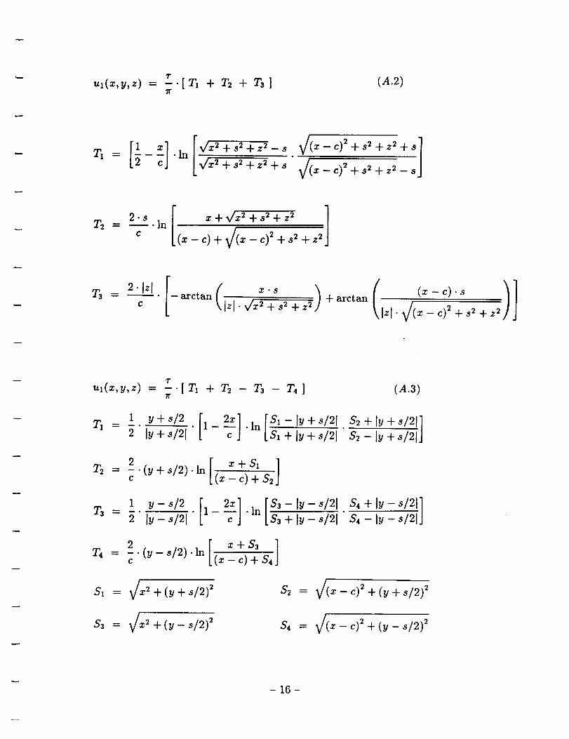
Ul(X,_,Z ) = T. [ T17/"

+ r2 + T3] (.4.2)

2"ST_ = _-ln

¢

In

_ _)+ V/(__ _)2+ _ + ,_

arctan (j z x-s )J. v/z_ + s2 + z_ + arct an

I" 7(z - c)2+ s2 + z_

u,(z, y, z) = r-_'[T, + T2 - T3 - T4] (A.3)

: Y+s/2 I ._] [s_-Iy+s/21.T1 -- : " lY + s/2_ " 1- .In $1 + ly + s/2i

- [ _+s, lT2 = 2 . (y + s/2) . ln (z - c) + S_C

S_-ly+ s/21J

T3 = :.]y s/21. 1- -In _7_- _ S4-ly-s/2lJ

T, = -2.(_,-_/2)._[ _+s, ](_-_)+&.l

S, = 7x 2+(y+s/2) 2

S3 z + (y - s/2) 2

- 16-

,,1(_,_,_) = _-.[T, + T_] (AA)71"

2"3T2 = --. In

c

u_(x,y,z) = v_.[ TI + T2 + T3 - T4] (A.5)7I"

2"i = 2"ly+s/21"In .............

2T3 = -.(y+ s/2).in

C

2T4 = -" (y- s/2). In

C

+ _/_2+ (u - _,/2)_"ly- _/21

-17-

APPENDIX B

CALCULATED LIMITS

)ira I_+s/21J= 1 (B._)

lim$"--_ OO

y - s/2 ])i% ly-,,/=l = -1

_/(_- _)_+ (y±_/2)_+/y__t/21]_/_ + (y + _/2)_+ ly+ .,/21 J

= 1

(B.2)

(B.3)

lim$'--_ OO

_/=2+ (y+ ,/2)_ _ I_+ s121

¢(z - c) 2 + (y + s12) _ - tu + s/21

x 2D

(x -c) _(B.4)

lim$---.* OO (y + s/2). In

+ _/x=+ (_ + ,/2) 2

(_ - _)+ V/(x- _)=+ (_ + ,/2) =¢ (B.5)

lim$"-* Oo (y-s/2).

In : + + :'/2/Z(x - c) + 7(= - c)2 + (y - s/2) _

--c (B.6)

- 18-

APPENDIX C

ANALYTIC FLOW FIELD SOLUTION (WAKE)

C_e No.

1

2

3

Condition

z#Oorz =0and

z # x, and z # z, + c°

z =0 and

x =xs or x = xs "-}-cs and

lyl> b_/2z=O and

x = x, or x = x, + c, and

lyl < bw/2

Solution

Eq. (C.1)

Sq. (C.2)

singular

u2(x,y,z) = q.[A1 - A2 ]47r

r._ .T --X t /

A, . [

_/(x - x,) _ + (y - b_12) 2 +

y+b_/2

V/(x - x,) 2 + {Y + b,,,/2) _ +

y - bw/2 ]

Jz 2

(c.1)

Z 2

x. - x, - c, [ y + b_/2_t_= (__ _. 2_:-)_+ z_" _f(__ _o_ _,1_+ (_+ b_/2)_+ _

_ y-b_,/2 ]_/(_ - _° - _,)' + (y - b_/2)2+ _

u_(z,u,z) = q. 147r ¢s

y+b,_/2 y-bw/2

V/c,_ + (u + b,,,/2)2 V/C, :2+ (Y - b_/2) 2°

(C.2)

- 19 -