A Visual Approach to Analysis of Stress Tensor Fields · ZIB REPORT: SUBMITTED AUGUST 31, 2010 1 A Visual Approach to Analysis of Stress Tensor Fields Andrea Kratz, Bjorn Meyer, and

Takustraße 7D-14195 Berlin-Dahlem

GermanyKonrad-Zuse-Zentrumfur Informationstechnik Berlin

ANDREA KRATZ, BJORN MEYER, INGRID HOTZ

A Visual Approach to Analysis of StressTensor Fields

Submitted August 31, 2010

ZIB-Report 10-26 (August 2010)

ZIB REPORT: SUBMITTED AUGUST 31, 2010 1

A Visual Approach to Analysisof Stress Tensor Fields

Andrea Kratz, Bjorn Meyer, and Ingrid Hotz

Abstract—We present a visual approach for the exploration of stress tensor fields. Therefore, we introduce the idea of multiple linkedviews to tensor visualization. In contrast to common tensor visualization methods that only provide a single view to the tensor field, wepursue the idea of providing various perspectives onto the data in attribute and object space. Especially in the context of stress tensors,advanced tensor visualization methods have a young tradition. Thus, we propose a combination of visualization techniques domainexperts are used to with statistical views of tensor attributes. The application of this concept to tensor fields was achieved by extendingthe notion of shape space. It provides an intuitive way of finding tensor invariants that represent relevant physical properties. Usingbrushing techniques, the user can select features in attribute space, which are mapped to displayable entities in a three-dimensionalhybrid visualization in object space. Volume rendering serves as context, while glyphs encode the whole tensor information in focusregions. Tensorlines can be included to emphasize directionally coherent features in the tensor field. We show that the benefit of sucha multi-perspective approach is manifold. Foremost, it provides easy access to the complexity of tensor data. Moreover, including well-known analysis tools, such as Mohr diagrams, users can familiarize themselves gradually with novel visualization methods. Finally, byemploying a focus-driven hybrid rendering, we significantly reduce clutter, which was a major problem of other three-dimensional tensorvisualization methods.

Index Terms—

F

1 INTRODUCTION

The focus of this work is the analysis and visualizationof 3D stress tensor fields, which express the response of amaterial to applied forces. Important application areas andtheir interest in such data are: In material science, a material’sbehavior under pressure is observed to examine its stability.Similar questions also arise in astrophysics. Rock fracturescaused by tension or compression, for example, are analyzedin geosciences. A medical example is the simulation of animplant design’s impact on the distribution of physiologicalstress inside a bone [1]. Common to most of these areasis the goal of finding regions where the inspected materialtends to crack. Various failure models exist, but in generalthey are based on the analysis of large shear stresses. Besidesunderstanding a physical phenomenon, tensor analysis canhelp to detect failures in simulations where tensors appear asintermediate product. In all these application areas, regionsof interest are not necessarily known in advance. For thisreason, powerful visual exploration and analysis tools are ofhigh importance.

The complexity of tensor data makes them hard to visualizeand interpret. Therefore, users tend to analyze tensor datavia two-dimensional plots of derived scalars (data reduction).Although these plots simplify the analysis at first glance, theydo not communicate the evolution of tensors over the wholefield [2]. They might even fail to convey all informationgiven by a single tensor. From a visualization point ofview, the difficulty lies in depicting each tensor’s complexinformation, especially for three-dimensional tensor fields.

• A. Kratz, B. Meyer and I. Hotz are with Zuse Institute Berlin.E-mail: [email protected], [email protected] and [email protected]

Often, visualizations are restricted to two-dimensional slices(data projection), as three-dimensional visualizations tend toresult in cluttered images. However, data reduction and dataprojection both reduce the complex information of the tensorfield to a small subset. Thus, the richness of the data is notcommunicated.

A further challenge, for example in contrast to vector fieldvisualization, is the young tradition of advanced tensor visu-alization methods in the considered application areas. Usersneed to get used to the advantages of modern visualizationtechniques, and therefore need tools to explore the data sothey can develop an intuition and construct new hypotheses.Therefore, it is important to link methods domain experts arealready used to with novel techniques. The main challengesin visualizing three-dimensional tensor fields, and the resultinggoals of our work are:

• Tensor data are hard to interpret. Thus, we provide anintuitive approach to the analysis of tensor data.

• Tensor visualization methods do not have a long traditionin their respective application areas. Thus, we providewell-known perspectives onto these data and link themwith novel visualization methods.

• A lack of a-priori feature definitions prevents the use ofautomatic segmentation algorithms. Thus, we allow usersto find the unknown and let them steer the visualizationprocess.

• The stress tensors we are dealing with are symmetric3D tensors described by six independent variables. Thus,effectively capturing all of this information with a singlevisualization method is practically not feasible. We there-fore employ a feature-dependent hybrid visualization.


ContributionTo meet these goals, we present a new access to tensor fields.The major contributions of this paper are:• Introduction of shape space theory as basic means for

feature designation in attribute space. Previous workmostly concentrated on the properties of a specifictensor type. We introduce an intuitive way of findingtensor invariants that reflect relevant features. Buildingupon the idea of shape space, the challenging task oftranslating questions into appropriate invariants boilsdown to a basis change of shape space. Using conceptsfrom stress analysis and including failure models, wepresent invariants for stress tensor fields together withcommon and new visualization techniques (Figure 2).However, our approach is extendable to the analysis ofvarious types of symmetric second-order tensors.

• Introduction of multiple linked views to tensor visual-ization. Previous work mostly concentrated on only twodimensions and/or one particular visualization technique.We pursue the idea of providing various perspectivesonto the data and propose visual exploration in attributeand object space. The concept of shape space servesas link between the abstract tensor and its visualizationin attribute space. In object space, features are mappedto displayable entities and are explored in a three-dimensional hybrid visualization.

2 RELATED WORK

Besides work from tensor field visualization [3], our work isbased on publications from multiple view systems [4] as wellas from the visualization of multivariate data [5]. This reviewis structured according to our main contributions focusing onsecond-order stress tensors and their visualization in attribute(diagram views) and object space (spatial views).

Tensor Invariants: Central to our work is the finding thattensor visualization methods can be designed and parametrizedby a specific choice of invariants, which are scalar quantitiesthat do not change under orthogonal coordinate transformation.Considering and analyzing important invariants is commonin many physical applications [6]. For analysis of diffusiontensors, [6] has been transferred to visualization [7]. Inthe same context, Bahn [8] came up with the definition ofeigenvalue space, where the eigenvalues are considered to becoordinates of a point in Euclidean space. In this work, weuse the term shape space referring to application areas suchas vision and geometric modeling. Coordinates within thisspace describe a set of tensor invariants and are called shapedescriptor.

Diagram Views: Only few visualization papers arerelated to using diagram views for tensors. Mohr’s circle [9]is a common tool in material mechanics, being used tocompute coordinate transformations. In visualization, it hasbeen applied to diffusion tensors to depict the tensor’sdiffusivity [10] as well as to stress tensors [11]. Being a

known technique for domain experts, Mohr diagrams canease the access to novel visualization methods. Directionalhistograms have been used to visualize the distribution offiber orientations in sprayed concrete [12] and for diffusiontensors in terms of rose diagrams and 3D scatterplotsof the major eigenvector angles [13]. To the best of ourknowledge, combined views for tensors have not beenpresented previously.

Spatial Views: A common classification of spatial visu-alization methods for second-order tensors is to distinguishbetween local, global and feature-based methods.

Local methods use geometries (glyphs) to depict singletensors at discrete points. Shape, size, color and transparencyare used to encode tensor invariants. Dense glyph visualiza-tions use less complex geometries together with placementalgorithms [14], [15], [16]. When only selected locations areexamined (probing), more complex geometries can be used.A variety of glyph types have been presented, focusing onstress tensors [2], higher-order tensors [17] and perceptualissues [18], [19]. Although, local methods have the potentialto depict the whole tensor information, they generally fail ingiving an overview of the complete 3D tensor field.

In contrast, global methods present an overview and empha-size regional coherence. They can be classified into methodsbased on scalar and vector visualization, as well as hybridmethods. Scalar visualization methods that are used to visual-ize tensors are ray-casting [20], [21], [22] and splatting [23],[24]. The main challenge is the design of an appropriatetransfer function. Kindlmann et al. [20], [21] define an opacitytransfer function based on the isotropic behavior of the tensorfield. Color and shading are defined by tensor properties suchas orientation and shape. Inspired by this work, Hlawitschka etal. [22] focus on directional information for transfer functiondesign to emphasize fiber bundle boundaries. Recently, Dicket al. [1] presented a colormapping for stress tensors in orderto distinguish between compressive and tensile forces.

Vector visualization methods are used to depict the behaviorof the eigenvectors. We distinguish line tracing algorithmslike tensorlines [25], texture-based approaches such as LineIntegral Convolution (LIC) [26] and reaction-diffusion tex-tures [27], [21]. Hotz et al. [28] presented a LIC-like methodfor the visualization of two-dimensional slices of a stresstensor field. They introduce a mapping of the indefinite stresstensor to a positive-definite metric. The mapped eigenvaluesthen are used to define input parameters used for LIC.

Whereas scalar-related visualization techniques are able tocover aspects of the whole 3D field, vector-related methodsare mostly restricted to two dimensions. Hybrid approachescombine global and local methods [29], [30] as well as scalar-and vector-related techniques [1], [31]. Dick et al. [1] proposedhybrid visualization for 3D stress tensor fields. They combineray-casting of the three eigenvalues with tensorlines to depictselected directions. To account for clutter, tensorlines are onlyseeded on a surface mesh. Although some hybrid approachestry to combine complex focus with non-disruptive contextvisualization, none of the existing methods allows the analysisand visualization of a complete 3D field both in detail and at


Raw tensor datadi

agon

aliz

e Invariant Selection (Question/Task)

EigenvaluesShape Space

TransformationShape Descriptors

Directional Invariants

Orientation SelectionEigenvectors

Shape Space

Object Space

Raycasting

Tensorlines

Glyphs

Attribute Space

ScatterplotMohr Diagram

Directional HistogramDirectional Scatterplot

Interaction loop #1

Mask Volume

Interaction loop #2

createupdate

evaluate

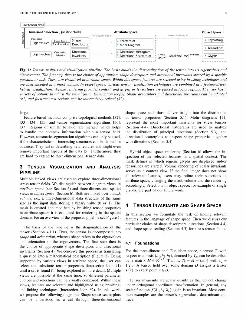
Fig. 1: Tensor analysis and visualization pipeline. The basis builds the diagonalization of the tensor into its eigenvalues andeigenvectors. The first step then is the choice of appropriate shape descriptors and directional invariants steered by a specificquestion or task. These are visualized in attribute space. Within this space, features are selected using brushing techniques andare then encoded in a mask volume. In object space, various tensor visualization techniques are combined in a feature-drivenhybrid visualization. Volume rendering provides context, and glyphs or tensorlines are placed in focus regions. The user has avariety of options to adjust the visualization (interaction loops): Shape descriptors and directional invariants can be adapted(#1) and focus/context regions can be interactively refined (#2).

large.Feature-based methods comprise topological methods [32],

[33], [34], [35] and tensor segmentation algorithms [36],[37]. Regions of similar behavior are merged, which helpsto handle the complex information within a tensor field.However, automatic segmentation algorithms can only be used,if the characteristics of interesting structures can be defined inadvance. They fail in describing new features and might evenremove important aspects of the data [5]. Furthermore, theyare hard to extend to three-dimensional tensor data.

3 TENSOR VISUALIZATION AND ANALYSISPIPELINE

Multiple linked views are used to explore three-dimensionalstress tensor fields. We distinguish between diagram views inattribute space (see Section 5) and three-dimensional spatialviews in object space (Section 6). Both are linked over a maskvolume, i.e., a three-dimensional data structure of the samesize as the input data storing a binary value (0 or 1). Themask is created and modified by brushing tensor propertiesin attribute space; it is evaluated for rendering in the spatialdomain. For an overview of the proposed pipeline see Figure 1.

The basis of the pipeline is the diagonalization of thetensor (Section 4.1.1). Thus, the tensor is decomposed intoshape and orientation, whereas shape refers to the eigenvaluesand orientation to the eigenvectors. The first step then isthe choice of appropriate shape descriptors and directionalinvariants (Section 4). We conceive this process as translatinga question into a mathematical description (Figure 2). Beingsupported by various views in attribute space, the user canselect and substitute tensor properties (interaction loop #1)until a set is found for being explored in more detail. Multipleviews are possible at the same time, so different parameterchoices and selections can be visually compared. Within theseviews, features are selected and highlighted using brushing-and-linking techniques (interaction loop #2). In this work,we propose the following diagrams: Shape space scatterplotscan be understood as a cut through three-dimensional

shape space and, thus, deliver insight into the distributionof tensor properties (Section 5.1). Mohr diagrams [11]represent the most important invariants for stress tensors(Section 4.4). Directional histograms are used to analyzethe distribution of principal directions (Section 5.3), anddirectional scatterplots to inspect shape properties togetherwith directions (Section 5.4).

Hybrid object space rendering (Section 6) allows the in-spection of the selected features in a spatial context. Themask defines in which regions glyphs are displayed and/ortensorlines are started. Volume rendering of scalar invariantsserves as a context view. If the final image does not showall relevant features, users may refine their selections inattribute space, changing the mask volume and the renderingaccordingly. Selections in object space, for example of singleglyphs, are part of our future work.

4 TENSOR INVARIANTS AND SHAPE SPACE

In this section we formulate the task of finding relevantfeatures in the language of shape space. Then we discuss ourparticular choice of shape descriptors, directions (Section 4.4)and shape space scaling (Section 4.3) for stress tensor fields.

4.1 Foundations

For the three-dimensional Euclidean space, a tensor T withrespect to a basis (b1,b2,b3), denoted by Tb, can be describedby a matrix M ∈ R3×3. That is, Tb = M = (mi j) with i,j =1,2,3. A tensor field over some domain D assigns a tensorT (x) to every point x ∈ D.

Tensor invariants are scalar quantities that do not changeunder orthogonal coordinate transformation. In general, anyscalar function f (λ1,λ2,λ3) again is an invariant. Most com-mon examples are the tensor’s eigenvalues, determinant andtrace.


Question Shape Orientation

InvariantsScaling Visualization Technique

Attribute ObjectSpace

σ₁,σ₂,σ₃ Scatterplot X

X

X

X

X

Logarithmic (SP)Distinguish regions of compression, expansion,shear and isotropic regions.

τ, R Logarithmic (SP) ScatterplotExplore regions of high shear and kind of anisotropy.

τ Linear (SP) HWY GlyphDepict the magnitude of shear stress acting at a givenpoint in any direction.

τ, c, R Linear (SP) Mohr DiagramDistinguish regions of compression, expansion, shear. Kind of anisotropy. Tensor as a whole.

e₁,e₂,e₃ - Directional HistogramDistribution of principal directions.

(e₁±e₃)

(e₁±e₃)

- Directional HistogramDistribution of directions of maximum shear stress.

X

X

X

f(σ₁,σ₂,σ₃) Linear (SP) Volume RenderingProvide a spatial context by means of a derivedscalar field.

σ₁,σ₂,σ₃

FA, mode(T)

e₁,e₂,e₃

e₁,e₂,e₃

Asymmetric (POS) Ellipsoid GlyphEncode whole tensor information in focus regions.

X

X

σ₁,σ₂,σ₃ Linear (SP) Reynolds GlyphDepict the normal stress acting at a given point in any direction.

e₁,e₂,e₃

e₁,e₂,e₃

- TensorlinesEmphasize selected directions.

XNormalized Superquadric GlyphDTI example: Which regions exhibit high anisotropy,and do they have a characteristic shape?

Fig. 2: Invariant Selection. The table gives examples for shape descriptors and directional invariants that correspond to aspecific task or question. We mainly present invariants for stress tensors. However, our approach is extendable to various types ofsymmetric second-order tensors. Besides convertible invariants, the analysis of tensors from diverse application areas requiresvariable scalings. The abbreviations SP and POS refer to sign-preserving mappings (SP) and mappings into a positive-definitemetric (POS), respectively. Furthermore, the table lists possible visualization techniques in attribute and object space.

4.1.1 Tensor DiagonalizationTensors are invariant under coordinate transformation, whichdistinguishes them from matrices. That is, the characteristicsof the tensor stay the same, independent from the choiceof basis. Consequently, a tensor can be analyzed using anyconvenient coordinate system.

In the following, we only consider symmetric tensors, i.e.,mi j =m ji, being defined by six independent components. Theycan be transformed into a principal coordinate system usingthe concept of eigenanalysis

U T UT =

λ1 0 00 λ2 00 0 λ3

. (1)

The diagonal elements λi are the eigenvalues and the trans-formation matrix U is composed of the eigenvectors ei. Forsymmetric tensors, the eigenvalues are all real, and the eigen-vectors constitute an orthonormal basis. They are ordered suchthat λ1 ≥ λ2 ≥ λ3.

4.1.2 Stress TensorA stress tensor conveys information about the stress acting oncutting planes through a material (Figure 3). It is given as

σ =

σ11 τ12 τ13τ12 σ22 τ23τ13 τ23 σ33

, (2)

with the diagonal components σi j being the normal stresscomponents and the off-diagonal components τi j the shearstress components respective to cutting planes normal to thecoordinate axis. The sign of the normal stress components

σ33

σ33

σ22

τ13τ23

τ13τ23

b1

b3

b2

n

t

σnτ

f

f

f

Fig. 3: External forces f that are applied to a material (left),stress measured on an infinitesimally small volume element(middle), and force (traction t) acting on an cutting planewith normal vector n (right).

encodes if they are compressive or tensile. In this paper, weinterpret negative eigenvalues as compressive forces (makingthe volume smaller) and positive eigenvalues as tensile forces(expanding the volume). It is worth noting that in someapplication areas the sign is interpreted in a reverse way. Ifforces are balanced and there is no rotation (which is, ingeneral, fulfilled for infinitesimally small volume elements),the tensor is symmetric and uniquely described by its threeeigenvalues and eigenvectors (Equation (1)). In this context,the eigenvectors are called principal stress axes, and theeigenvalues are called principal stresses. As principal stressesmay be positive or negative, the tensor is indefinite. The force(traction vector) t acting on a cutting plane with normal vectorn is given by

t = σ ·n = τ +σn. (3)

It can be decomposed into its normal stress σn and shear stresscomponent τ (Figure 3, right). In cutting planes orthogonal


(a) Linear σ3 ≈ σ2 < σ1; R≈ 1 (b) Planar σ3 < σ2 ≈ σ1; R≈ 0 (c) Isotropic σ3 ≈ σ2 ≈ σ1

Fig. 4: Lame’s stress ellipsoid (displaying all possible traction vectors) and Mohr’s circle in comparison. The ellipsoid’s axisare aligned with the three eigenvectors, which are scaled by the eigenvalues. For three-dimensional tensors, Mohr’s circleconsists of three circles drawn between the three eigenvalues [11]. The horizontal axis depicts the normal stress and thevertical axis the shear stress. The outer circle gives an impression of the maximum shear stress, i.e., the larger the circle, thegreater the shear stress acting on that plane. The blue shaded area represents all possible combinations of normal and shearforces for a given cutting plane. A point within this region then corresponds to the orientation of the plane’s normal.

to the principal directions the shear stress vanishes. Forplanes with normals bisecting the minimum and maximumprincipal direction, the shear stress takes its maximum valueand is called maximum shear stress τmax. The correspondingdirections are called direction of maximum shear stress.

4.2 Shape SpaceWe use the term shape space for the vector space spannedby the three eigenvalues. In this space, tensor shape [7] isrepresented by a point, whose coordinates are called shapedescriptors. Finding shape descriptors, suiting the initial ques-tion, then corresponds to finding an appropriate referenceframe (Figure 5). Common orthogonal reference frames cor-respond to Cartesian, spherical, and cylindrical coordinates,respectively. An example for a complete orthogonal spheri-cal invariant set commonly used in the context of diffusiontensor imaging (DTI) is [7]: tensor norm (radius), fractionalanisotropy (polar angle) and tensor mode (azimuthal angle).These descriptors represent central physiological properties(Figure 2). It is worth noting that all angular coordinatescorrespond to relative entities and are not defined in the origin(norm(T )2 = λ 2

1 +λ 22 +λ 2

3 = 0). For tensors with small norm,these values are unstable and sensitive to small changes. Asa consequence, such coordinate systems are not optimal forindefinite tensors, for which the characteristic invariants maybe positive, negative, or equal to zero (Section 4.1.2).

An additional useful property of a reference frame is orthog-onality. Orthogonal invariants exhibit maximum independenceof the shape descriptors by isolating changes of one invariantfrom variations of the others.

Which shape descriptors to use may depend on a variety ofcriteria. We propose the use of descriptors that give answersto specific questions and that are familiar to domain-experts.These criteria do not necessarily coincide with the mathemat-ically most appealing choices.

4.3 Shape Space ScalingThe scale of the shape space’s coordinate axes has a highimpact on the visualization result. Therefore, it plays a crucialrole in the diagram views (Section 5), as well as for renderingin the spatial domain (Section 6), where tensor invariantsdefine color, transparency, glyph shape and glyph size. Most

common visualization methods require positive values, whichis challenging for indefinite tensors, where the sign of theinvariants reveals important physical characteristics. On theother hand, most diagram views are based on positive as wellas negative eigenvalues. An optimal mapping depends on thegiven dataset and the desired visualization. It is possible toapply the mapping before choosing appropriate shape descrip-tors (holds for relative entities), or afterwards. We distinguishbetween the following mappings:• Sign-preserving mappings (SP): Examples are linear and

logarithmic mappings (Equation 6) as well as histogramequalizations.

• Mapping to R+ (POS) [28], [38]: Values are mapped tothe positive domain in a way that keeps the distinctionbetween positive and negative values (Equation 7).

These mappings are further discussed in Sections 5 and 6 in thecontext of the specific visualization methods. The eigenvectorsare already normalized and, therefore, do not need a mapping.

4.4 Shape Descriptors and Directions for StressTensorsTypical questions related to stress tensors are concernedwith stability and failure analysis. Therefore, most failuremodels build on the analysis of the maximum shear stress.An example is the Coulomb-Mohr failure criterion [39].Assuming no internal friction (µ = 0), it states that a materialyields as long as the maximum shear stress τ falls below theintrinsic shear strength τ0 of the material. Figure 6 depictsthis failure criterion graphically. As long as Mohr’s circle(Section 5.2) does not intersect the failure line, the inspectedmaterial does not fracture. The normal of the correspondingfracture plane is the angle bisector of the principal directionsof σ1 and σ3: the direction of maximum shear stress. Thematerial parameters µ and τ0 are measured in experiments.

Shape descriptors corresponding to the Coulomb criterionare [39]:

τ =σ1−σ3

2maximum shear stress

c =σ1 +σ3

2

R =σ1−σ2

σ1−σ3shape factor.

(4)


For other failure models, other shape descriptors exist. Ingeneral, these sets are not simple orthogonal coordinateframes, but represent important physical quantities.

Considering Mohr’s circle, c represents its center, and τ

its radius (Figure 5). The shape factor R ∈ [0,1] reveals thekind of anisotropy. Similar to the terminology used in DTI,stresses with R = 0 are called planar and R = 1 are calledlinear (Figure 4). It is a relative value and undefined forsmall values of τ (isotropic stresses).

An example for another common anisotropy measure con-sidering all principal stresses is the von Mises stress

σv =√

0.5 · ((σ1−σ2)2 +(σ2−σ3)2 +(σ1−σ3)2). (5)

σ1

σ3

σ2(a) Shape Space

c

τ

R(b) Circle Parameters

σn

τ

(c) Mohr’s Circle

Fig. 5: Shape Space Transformation using the example ofMohr’s Circle. The shape space (a) is spanned by the major(x-axis), minor (y-axis), and medium eigenvalue (z-axis). Thetensor’s shape is represented by a point. A circle is describedby its center c and its radius, which corresponds to themaximum shear τ . These shape descriptors are computed bya change of basis, which corresponds to a rotation aroundthe σ2-axis by 45 degrees (b). A final step corresponds toa mapping of (τ,c,R) to glyph geometry (c), whereas Rdistinguishes planar and linear stresses.

τ0+μσn

τ0

τ

σn

(σ1−σ3)/2

σ1

σ1

σ3

σ3

θθ

2θ

σ1σ2σ3

Fig. 6: Coulomb-Mohr failure criterion: The red area indicatesnormal-shear force combinations leading to material failure(left). The relation between the principal stress directions σ1and σ3 and the predicted fracture plane are given by the angleθ .

5 DIAGRAM VIEWS

We propose several diagram views, presenting various perspec-tives onto (stress) tensor characteristics (Figure 2). The views

abstract from the tensor volume’s spatial representation, andgive insight into the statistical distribution of tensor properties.All attribute-space views are linked and can be used side-by-side. Brushing in the views creates and updates a mask volumethat is used to assign visualization methods in the spatial view(Section 6). The diagram views are parameterized by:• Choice of shape descriptors.• Choice of directions.• Choice of shape space scaling.

In this section, we offer a default selection of views andparameterizations for the failure analysis of stress tensors. Ofcourse, a wide range of other parameter choices correspondingto the underlying application and data is possible, too.

Statistical views (e.g. scatterplots, histograms) are especiallysuitable to quantify tensor characteristics. We have adaptedscatterplots to fit scalar (Section 5.1) as well as directionaltensor invariants (see Section 5.4). Directional histogramsquantify selected directions, as eigenvectors or the directionof maximum shear. Furthermore, we present Mohr diagrams(Section 5.2) as additional perspective on the tensor data. Theyare a common tool in engineering, and therefore familiar toa large group of users. Compared to quantitative techniques,they give a more detailed view onto single tensors.

5.1 Shape Space ScatterplotA scatterplot is used to depict the relation between two scalarinvariants. Figure 7 illustrates a scatterplot that is used toquantify normal (compressive or tensile) and shear stresses.The input, therefore, are the three principal stresses sorted indescending order, i.e., σ1 ≥ σ2 ≥ σ3. The plot is divided intofour quadrants (A,B,C,D). Due to the ordering, there neverwill be any points in the upper left quadrant (A). Points inthe upper right quadrant (B) correspond to eigenvalues thatare all positive, characterizing tensors of high tensile stresses.Accordingly, points in the lower left quadrant (C) correspondto high compressive stresses. The most interesting region is thelower right quadrant (D), which shows tensors with tensile andcompressive stresses.

To summarize, we can deduce the following tensor fieldcharacteristics from the (σ1,σ3)-scatterplot:• The more points in quadrant B, the higher the level of

expansion.• The more points in quadrant C, the higher the level of

compression.• The more points in quadrant D, the higher the level of

mixed stresses.• Points that have a large distance to the isotropic axis

exhibit a high level of shear.• Points that are located near the isotropic axis exhibit no

shear at all; they describe tensors with isotropic behavior.For the scatterplot, there is no need for a mapping into the

positive domain. In contrast, an explicit distinction betweenpositive and negative scalar invariants can be important. Wepropose two sign-preserving mappings: Logarithmic and his-togram equalization [40]. As a standard logarithmic mapping


σ1

σ3 ≤ σ1 < 0 σ3 < 0,σ1 > 0

σ3

σ3 ≤ σ1 > 0

Fig. 7: Schematic illustration of the scatterplot (left). Thex-axis represents the major eigenvalue and the y-axis theminor eigenvalue. The medium eigenvalue is color-coded (bluedenotes low, red denotes high values). Example scatterplot forthe two-force dataset (right); a simulation of a cube affected bya pushing and a pulling force, which results in compressive aswell as tensile stresses. The eigenvalues were logarithmicallymapped (Equation 6).

has a singularity in zero, we use

f (σi) =

{log(σi +1), for σi ≥ 0− log(1−σi), for σi < 0.

(6)

The results are then linearly mapped to the range of -1 to1. In order to see as many tensor characteristics as possible,often a logarithmic mapping is sufficient. For some datasets,however, the data remain cluttered after the mapping. In thiscase, a histogram equalization is useful. Our modular approachallows an interactive adjustment of the mapping to the needsof the underlying dataset.

σ1

σ3

(a) (σ1,σ3)

τR = 0.5

planar

linear

(b) (τ,R)

min(σ2) max(σ2)

Fig. 8: Scatterplot for the slit-cube dataset (Section 7) withvarying shape descriptors as input. (a) Considering (σ1,σ3)as input, regions of compression, expansion and shear canbe distinguished. The inspected dataset exhibits mostly highshear stresses, no compressive forces and marginally tensileforces. Therefore, we analyze the shear region (Quadrant D) inmore detail (b) considering (τ,R). Plotting the shape factor Rreveals that within this region more linear (R≈ 1) than planar(R≈ 0) behavior happens.

5.2 Mohr DiagramFigure 9 illustrates the Mohr diagram, which is used toanalyze selected tensors in more detail. It consists of Mohr

circles (Figures 4 and 6), which give an impression of therelationship between the three eigenvalues and their relativestrength. The circle’s position on the x-axis indicates whetherthe respective tensor exhibits tensile or compressive forces. Itsradius expresses the level of shear. In the original diagram [11],most circles would be located around the origin. This is aregion of high interest as it represents high shear and suddenchanges from tensile to compressive stresses. To equalizethe circles’ distribution, we exploit that, in general, a Mohrdiagram is only one-dimensional; all circles are centered atthe x-axis. We categorize the circles according to the tensor’sanisotropic behavior (isotropic, linear, planar), and dividethe Mohr diagram into three separate diagrams (Figure 9).Thus, clutter around the origin is reduced significantly. Bydrawing semi-circles in context regions, we achieve a morecompact visualization without losing information or clarity.To summarize, we can deduce the following conditions fromthe Mohr Diagram:

• The more circles on the left, the higher the level ofcompression.

• The more circles on the right, the higher the level ofexpansion.

• Circles around the origin exhibit both: compressive andtensile forces.

• The greater the circle’s radius, the higher the level ofshear.

• Circles degenerating to a single point exhibit no shear atall; they describe tensors with isotropic behavior.

• A high number of circles on one of the threecategorization axes represents a high number ofisotropic/linear/planar tensors.

σ3 = σ2 = σ1

R≥ 0.5

R < 0.5

σi < 0 σi > 0

Fig. 9: We extended the Mohr diagram proposed by [11] asdepicted above. The circle’s position on the x-axis representswhether the corresponding tensor is in compression (left)or tension (right). The vertical position corresponds to theiranisotropic behavior. For a better overview, we only drawsemi-circles.

Due to its usability for the analysis and depiction of a singletensor or only a few tensors, the Mohr diagram is best usedafter a selection has been specified in the other diagram views.We achieve a further reduction of Mohr circles to be displayed,by clustering tensors with similar eigenvalue behavior. Assimilarity measure we use the Euclidean distance between twopoints in shape space. In the Mohr diagram, we encode thenumber of occurrences by color (Figure 13).


5.3 Directional HistogramFigure 10 illustrates the directional histogram, which is usedto analyze the distribution of principal shear directions. Ofcourse, other directions of interest can be inspected, too.An example is the directions of maximum shear stress.The spherical diagram projects each direction, for examplethe major eigenvector, onto the surface of a unit sphere.Due to the non-oriented nature of a symmetric tensor’sdirectional components only half of the sphere’s surfaceneeds to be considered. Therefore, all vectors are flippedto the positive half space of a user-selected axis (x,y,z). Tocreate the histogram, either a binning or a splatting approach[12] can be followed. We use the former. The number ofintersections between vectors and a given surface patch onthe sphere are counted, thus performing a region-dependentbinning. For accurate results, a uniform subdivision of thesurface is crucial. To account for patch size variations,we normalize the counted frequencies by the respectivepatch’s surface area. Given a triangulation of the unit sphere,we either bin by triangle or by the Voronoi cell of eachvertex. Triangle binning results in a discrete visualizationof the counted frequencies, where each triangle is coloreduniformly. Mapping the frequencies to vertex colors producesa continuous diagram, as the values are interpolated betweenneighboring vertices. The interpretation of the final plotdepends on the selected viewing direction. In the 2D plot, thediagram’s center corresponds to all vectors that are collinearwith this viewing direction. An arbitrary point on the sphere’ssurface represents all vectors that span the angles α andβ with respect to the two axes orthogonal to the selectedviewing direction (Figure 10).

We use two representations of the directional histogram(Figure 19):• Hemisphere• Mapping of the hemisphere into a planar representation

for a better depiction in 2D [41]

180° 0°

90°

0°

180°

α

β

(x, y, z)

(x, y, z)

(x, y, z)

0

P(α,β)

selected viewing axis

Fig. 10: The input directions for directional histogram anddirectional scatterplot are projected on a hemisphere, flippingall vectors to the half space defined by the selected viewingaxis. Each point P(α,β ) on the hemisphere represents all vectorsspanning the angles α and β .

5.4 Directional Scatterplot

The directional scatterplot uses the same setup of unit sphereand projected vectors as the directional histogram, but in-stead of binning the directions each vector is representedby an individual point on the sphere’s surface. This directrepresentation of the vectors allows using the point’s size,color, and transparency to represent tensor properties. Due tonumeric instabilities in simulations, isotropic tensors exhibitan increased noise ratio (Figure 11, a). To reduce the noiselevel in the plot and emphasize pronounced directions, wemap the shear stress to transparency. Thus, nearly isotropictensors do not contribute to the final plot (Figure 11, b).Reasonable quantities to be mapped to colors are normal andshear stresses.

(a) (b)

Fig. 11: Directional scatterplot for the rotating-star dataset.In Figure (a), all points have the same transparency, whichreveals artifacts due to isotropic tensors. In Figure (b) theshear stress is mapped to transparency, i.e., low transparencyfor low shear stresses and nearly opaque points for high shearstresses. Thus, nearly isotropic tensors do not contribute to theplot.

6 SPATIAL VIEWS

The spatial views represent the tensor field in its originalthree-dimensional coordinates. The most basic method todisplay tensors in a spatial context is to use graphical icons(glyphs), e.g. ellipsoids, that are placed at discrete pointswithin the volume. Although glyphs have the potentialto show the entire tensor information, they fail to give acontinuous view of the tensor field. Such a global view,however, is important to identify regions of compressionand expansion, respectively. Volume rendering methods givea global view of the tensor field. However, in general theyonly work on derived scalar values and thus do not containdirectional information. We use a hybrid rendering approach,combining volume rendering with glyphs and tensorlines. Thevisualization is interactively steered by a mask volume thatis created and updated through user selections in the diagramviews.

The basic idea is to use various visualization methods toseparate focus and context regions in the dataset. Therefore,we evaluate the mask volume and map the selected features


to geometrical tensor representations (glyphs, tensorlines). Thecontext is visualized by a volume rendering of the remainingdataset, using a scalar invariant chosen by the user.

Volume Rendering: Volume rendering serves as contextview with decreased opacity in focus regions, allowing toanalyze glyphs and tensorlines in more detail. We use standardGPU ray-casting of scalar invariants, for example, the vonMises stress. As tensorlines and glyphs are explicit geometries,we have to account for correct intersections between volumeand opaque scene geometry. As proposed by [42], we use adepth image of the geometry. During volume traversal, raysare stopped as soon as they hit geometry positions.

Tensorlines: To add directional information, tensorlinescan be drawn in focus regions, i.e., seeds are randomly placedinside the masked volume. Starting at these seed points, theline is integrated using a fourth-order Runge-Kutta scheme.The integration is stopped as soon as the line runs into anisotropic region.

Tensor Glyphs: Alternatively, glyphs can be drawn infocus regions, encoding the whole tensor information locally.Currently, we use ellipsoids. In order to distinguish betweenpositive and negative eigenvalues, we map the tensor to apositive-definite metric using an antisymmetric-mapping [28]:

f (σi,c,α) = exp(αarctan(c ·σi)). (7)

The parameter c determines the slope of the function in theorigin, α is a scaling parameter. The glyph’s size can beadapted using a global scale parameter.

7 RESULTS

We describe two visual analysis sessions by means oftwo datasets with diverse characteristics (Sections 7.1, 7.2).Whereas the slit cube simulation is an example where do-main experts have clear questions, the rotating-star datasetdemonstrates a case with less specific questions. All analyseswere performed on a standard desktop PC, equipped with anIntel Core 2 Duo CPU with 3.0 GHz and a NVIDIA GeForce8800GT GPU.

7.1 Exploring the Slit-Cube DatasetThe slit-cube dataset is generated via a finite element simu-lation of the deformation of a clamped cube with two slits.Surface forces are applied to the top and the side of thecube, which is fixed at the bottom. Figure 12 (a) illustratesthis process. The images are rendered based on a uniformresampling of the dataset. The resolution of the tensor fieldis 256×256×256. In this context, the stress tensor expressesthe cube’s response to the applied forces. Questions are:• How does the material respond to the applied forces?• Which forces act in the material?

In general, the von Mises stress σv, a scalar value that isderived from the stress tensor (Equation (5)), is used to predictyielding of materials. Regions where σv is high, are prone tomaterial failure.

Figure 12 (b) shows a spatial view of the dataset, using ahybrid rendering to visualize focus and context. A volume

(a) (b)min(σv) max(σv)

Fig. 12: Slit Cube. The dataset is based on a finite elementsimulation of the deformation of a clamped cube with two slits(a). It is fixed at the bottom. Surfaces forces act on the top andthe side of the cube. (b) Shows a hybrid rendering of the slit-cube dataset. Volume rendering of the von Mises stress servesas context, while ellipsoids oriented by the eigenvectors andscaled by the eigenvalues are positioned in focus regions toemphasize high shear stresses.

rendering of the von Mises stress gives an impression of thewhole field, while glyphs are positioned in focus regions andhighlight areas of extremely high stresses. It can be seen that,due to the applied forces, the cube’s slits increase. Largestresses are concentrated close to the edges of the slits and atthe bottom where the cube is fixed, while large areas of thecube are hardly affected by the applied forces.

The von Mises stress is easy to interpret, however,important information of the stress tensor is ignored. Thatis, we cannot say which forces are prevalent in the materialand we cannot say anything about the direction of maximumstresses.

The (σ1,σ2,σ3)-scatterplot (Figure 8) allows a distinctionbetween compressive, tensile and mixed stresses as well asisotropic and high shear stresses. It shows that the inspecteddataset exhibits mostly indefinite stresses, no compressiveforces and marginally tensile forces. Therefore, in the nextstep of the analysis, we switch the shape descriptors from(σ1,σ2,σ3) to (τ,R) using a logarithmical mapping (interac-tion loop #1) for the display (Figure 8). Thus, the shear region(Quadrant D) can be analyzed in more detail. Plotting themaximum shear stress against the shape factor R reveals thatthis region exhibits more linear than planar behavior. Linear,planar and isotropic stresses are further explored in the Mohrdiagram (Figure 13). The circles are color-coded according totheir frequency. Using the Mohr diagram as overview, we canreveal the physical behavior over the whole field. It is clearlyvisible that the slit-cube mainly exhibits indefinite stressesresulting in Mohr circles centered around the origin. However,looking at Figures 13 (b), (c) we can also deduce marginallycompressive and tensile forces. As compressive forces are onlysmall outliers in the scatterplot, we have not seen them before.

As we are especially interested in regions of high shearstress, we next examine the directions of maximum shear stress


(a) Overview (b) σi < 0 (c) σi > 0 (d) Zoom

# = 1 max(#)

Fig. 13: Slit Cube. The Mohr diagram (a) mainly reveals mixed stresses (circles around the origin) as already shown in thescatterplot. Figures (b) and (c) show regions of compressive (b) and tensile forces (c), respectively. Looking at the scatterplotalone, we deduced that no compressive forces appear in the dataset, as these are only small outliers. Zooming into the linearregion reveals more detail. The circles are colored according to their frequency (#).

(Figure 19). The directional histogram reveals one stronglyexpressed peak aligned with the z-direction. A second, minoraccumulation is smeared over a larger angle in x,y-plane, ap-proximately 90 degrees to the main stress direction. Figure 14shows a hybrid rendering, where additional tensorlines areseeded in regions of high stress following the major principalstress direction.

min(σv) max(σv)

Fig. 14: Slit Cube. The image shows a hybrid rendering of theslit-cube dataset. Volume rendering of the von Mises stressserves as context. Tensorlines are seeded in regions of highstress and integrated along the major eigenvector direction.

7.2 Exploring the Rotating-Star Dataset

Our second example shows data from an astrophysical simu-lation of a rotating neutron star’s dynamics. Analyzing theevolution of such systems plays a major role for the un-derstanding of the fundamental processes involved in corecollapse supernovae and gravitational wave production.

(a) (b)# = 0 max(#)

Fig. 19: Slit Cube. Directional histogram to examine thedistribution of the directions of maximum shear stress. Wemapped the hemisphere (front part of the sphere in (b)) into aplanar representation (a) for a better depiction in the paper.

The simulation results consist of a variety of data types,i.e., (complex) scalars, vector fields and tensors. The datais usually three-dimensional and time-dependent, given ona grid with spatially varying resolution (AMR). In thiswork, we focus on the second-order stress tensor field. Thedata is resampled on a uniform grid with a resolution of128×128×128 samples.

Until now, the domain experts’ examination focusedon the scalar fields (e.g. magnetic-, velocity- and densityfields), which give insight into the evolution of the starformation. Other data types arise as intermediate product ofthe simulation. The additional analysis of the stress tensorfield could support a deeper understanding of the physicalprocesses that cause this specific formation. Investigations are,for example, related to the forces that participate in the star’s


(a) t = 10 (b) t = 500 (c) t = 1580

Fig. 15: Rotating Star. The tensorlines are integrated along the major eigenvector direction. Following the lines shows that thestar’s rotation lags around its perturbation. The seed points were placed at the star’s center using a simple random seeding.

σ₁

increasi

ng

isotro

pic pressu

re

increasing maxshear stress

(a) t = 10

σ₁

(b) t = 500

σ₁

(c) t = 1580

min(τ) max(τ)

Fig. 16: Rotating Star. The scatterplot shows that, due to the perturbation, the forces get stronger with increasing time steps.The shape of the plot stays the same, which leads to the assumption that the eigenvalues correlate to each other. The colorrepresents the maximum shear stress τ .

(a) t = 10 (b) t = 500 (c) t = 1580

# = 0 max(#)

Fig. 17: Rotating Star. Directional histogram for the shear vectors. The colored triangles represent the number of data points(#) exhibiting a maximum shear direction falling into the triangle. At the beginning of the simulation (a) all shear directionsexhibit a specific angle, which is nicely depicted by a single circle in the diagram. In later time steps, the shear directionsbecome more scattered and the strongly expressed direction splits into two maxima rings (b). With further increasing time, thesetwo maxima merge again resulting in one dominant ring (c). According to our domain experts, the splitting is not physical. Itpossibly reveals discretization artifacts.

(a) t = 10 (b) t = 500 (c) t = 1580

min(λ1) max(λ1)

Fig. 18: Rotating Star. Hybrid rendering that combines volume rendering of the first tensor component with glyphs.Superquadrics are calculated only on the equatorial plane and colored according to the major eigenvalue λ1. As deducedfrom the scatterplot, the forces get stronger with increasing time steps resulting in larger ellipsoids revealing linear forces.

collapse. However, contrary to our first example (Section 7.1),questions are much more basic. Since the users are not usedto look at the tensor data, they do not have any specific

expectations. Therefore, the first goal of the visual explorationis to get an initial idea of the information that is contained inthe data. Besides the physical interpretation, a thorough data


analysis is of high importance to validate the quality of thesimulated data. Often, even simple visualizations can revealfailures in the simulations.

For a first impression of the dataset, Figure 15 displaystensorlines following the major eigenvector for three timesteps t. The lines are seeded close to the center of the star.

Figure 20 shows the Mohr diagram of the rotating-stardataset. Due to the high gravitational forces inside the star onlycompressive stresses occur. According to our sign conventionthis means that all stresses are negative. In such a case it iscommon in the respective application areas to consider onlythe absolute value of the stresses. The principal stresses are or-dered according to their magnitude, i.e., |σ1| ≥ |σ2| ≥ |σ3|. Asa consequence, the dataset reveals positive-definite behavior,which can be clearly seen in the Mohr diagram. An interestingobservation that can be made when zooming into the focusregions, is that the stresses exhibit perfectly linear behavior,i.e., the shape factor is R = 1.

# = 1 max(#)

Fig. 20: Rotating star. The Mohr diagram reveals only com-pressive forces, which are perfectly linear. According to oursign convention this means that all stresses are negative.In such a case it is common in the respective applicationareas to consider only the absolute value of the stresses. Theprincipal stresses are ordered according to their magnitude,i.e., |σ1| ≥ |σ2| ≥ |σ3| and, thus, restricted to the positivex−axis. In the selected region we draw full colored circles.

Figure 16 shows scatterplots for three time steps. As|σ1| ≥ |σ2| ≥ |σ3|, only positive stresses occur. Therefore,only quadrant B is displayed. It can be observed that afterthe initial perturbation the principal stresses |σ1|, |σ3| as wellas the shear forces get stronger with increasing time, i.e.,the distance to the isotropic axis increases (Figure 16 (c)).Interestingly the characteristic shape of the scatterplot staysthe same over a long period of time. This might lead to theassumption that the major and minor eigenvalue correlate toeach other. As we have seen in the Mohr diagram, all tensorsexhibit perfect linear behavior. Therefore, we can deduce thatthe major eigenvalue |σ1| grows almost quadratically withrespect to |σ2| and |σ3|.

A temporal analysis of the dominant shear directions canbe performed based on the directional histograms given inFigure 17. All time steps clearly reflect the symmetry inherentto the data set. At the beginning of the simulation (t = 10)all shear directions exhibit a specific angle, which is nicelydepicted by a single circle in the diagram. In later time steps,the shear directions become more scattered and the stronglyexpressed direction splits into two maxima rings (t = 500).With further increasing time, these two maxima mergeagain resulting in one dominant ring (t = 1580). Accordingto our domain experts, the splitting is not physical. As aconsequence, the visualization triggered a discussion aboutthe possible reasons for this development. First ideas includeddiscretization artifacts and problems with the resolution ofthe star’s surface.

Figure 18 shows a hybrid rendering of the dataset. Thevolume rendering uses the σ11 component of the tensor. Eventhough this is not an invariant it expresses a characteristictensor behavior, due to the high symmetry of the data. Therendering is combined with a glyph representation seeded inthe equatorial plane.

8 DISCUSSION

Our results demonstrate the application of the presentedpipeline (Figure 1) and shape space as basic means forfeature designation in attribute space (Section 4). We haveshown that the complexity of tensors can be embeddedinto a coherent concept, which builds the foundation forfuture research in tensor field visualization. Previous workmostly concentrated on one particular type of tensor andvisualization technique. Analyzing tensors from diverseapplication areas, which exhibit different properties, requiresconvertible invariants and variable mapping techniques.Figure 2 shows invariants for stress tensors, however, theunderlying concept can be used for other tensors, too. Asmotivated by our co-operation partners, future research willinclude the comparative visualization of different tensor typesthat occur during the same simulation (e.g. gravitational fieldtensor and stress tensor).

Our results and the discussion with domain expertsfurther confirm the need for powerful visual exploration andanalysis tools. The concurrent use of well known and newvisualization methods provides an access to both, the dataand modern visualization techniques. In material science andastrophysics, tensors are simulated solely to investigate scalarquantities (von Mises stress, density). Tensors mainly appearas intermediate product of simulations. Although, expertsknow that the tensor contains important information, whichmay help to answer their questions (What makes the materialcrack?, Which forces make the star collapse?), they avoidlooking at the complex data as they do not know how tointerpret it.

Until now, domain experts are mainly used to two-dimensional plots. Therefore, attribute-space plots are of


high importance. Our experience is that domain expertsfavor simple visualization techniques like scatterplots andicons that are familiar to them (e.g. Mohr’s circle). In objectspace, a sparse usage of lines and glyphs at specific locationsis preferred, which motivates the use of a binary maskvolume to determine focus and context regions. Moreover,all physicists and engineers rated the brushing-and-linking asextremely helpful to ease the interpretation of the data. Thatway, the visual exploration leads to new questions, whichencourages both, the curiosity to look at the whole tensorand, as a consequence, the development and usage of morecomplex visualization techniques. Another aspect that aroseduring discussions was the usefulness of our methods todetect failures in simulations.

Our material science partners really like the Mohr diagram;the familiar technique motivated them to use our tools. Forastrophysicists the representation was new but consideredas interesting. A limitation is that the diagram suffersfrom clutter. A clear distinction between linear and planaranisotropy in the tensor field is still difficult. Therefore, wewill integrate clustering algorithms in the future to revealmore insight into important tensor properties.

Another subject that remains to be investigated is volumerendering in the context of tensor fields. Users like thisvisualization technique as they know, how to interpret it. Thiswork presents renderings of scalar measures (e.g., von Misesstress). Recently, Dick et al. [1] presented a colormapping ofthe three eigenvalues to distinguish between compressive andtensile forces. More advanced colormappings based on othertensor invariants may be interesting, too.

9 CONCLUSION

To the best of our knowledge, we presented the first approachthat solves the challenging problem of visualizing three-dimensional tensor fields by combining multiple views. Asolid theoretical basis was provided by extending the notionof shape space, which serves as a link between the abstracttensor and its visualization in attribute space. This theoryprovides an intuitive way of finding relevant features.

In the considered application areas, visual tensor analysisand exploration are still in their infancy. Domain experts areoften used to the analysis of derived scalar fields, although theyknow that the tensor field contains important information totheir questions. Especially attribute plots help them to familiar-ize themselves with more advanced visualization techniques,explore the data and to construct new hypotheses.

ACKNOWLEDGMENTS

This work was funded by the German Research Foundation(DFG) through a Junior Research Group Leader award (EmmyNoether Program). Rotating-star data supplied courtesy ofLuca Baiotti from the Albert Einstein Insitute (AEI). The slit-cube dataset was provided by Andreas Schroeder, HumboldtUniversity Berlin. The authors would further like to thank

Markus Hadwiger, Aaryn Tonita, Michael Koppitz, SteffenProhaska and our students David Bressler and Nino Kettlitz.Finally, we thank the reviewers for their valuable comments.

REFERENCES

[1] C. Dick, J. Georgii, R. Burgkart, and R. Westermann, “Stress tensor fieldvisualization for implant planning in orthopedics,” IEEE Transactions onVisualization and Computer Graphics, vol. 15, no. 6, pp. 1399–1406,2009.

[2] Y. M. A. Hashash, J. I.-C. Yao, and D. C. Wotring, “Glyph andhyperstreamline representation of stress and strain tensors and materialconstitutive response,” International Journal for Numerical and Analyt-ical Methods in Geomechanics, vol. 27, no. 7, pp. 603–626, 2003.

[3] H. Hagen and C. Garth, “An introduction to tensors,” in Visualizationand Processing of Tensor Fields. Springer, 2006.

[4] H. Doleisch, M. Gasser, and H. Hauser, “Interactive feature specificationfor focus+context visualization of complex simulation data,” in VISSYM’03: Proceedings of the symposium on Data visualisation 2003. Euro-graphics Association, 2003, pp. 239–248.

[5] R. Burger and H. Hauser, “Visualization of multi-variate scientificdata,” in EuroGraphics 2007 State of the Art Reports (STARs), 2007,pp. 117–134. [Online]. Available: http://www.cg.tuwien.ac.at/research/publications/2007/buerger-2007-star/

[6] J. C. Criscione, J. D. Humphrey, A. S. Douglas, and W. C. Hunter, “Aninvariant basis for natural strain which yields orthogonal stress responseterms in isotropic hyperelasticity,” Journal of the Mechanics and Physicsof Solids, vol. 48, pp. 2445–2465, 2000.

[7] D. B. Ennis and G. Kindlmann, “Orthogonal tensor invariants andthe analysis of diffusion tensor magnetic resonance images,” MagneticResonance in Medicine, vol. 55, no. 1, pp. 136–146, 2006.

[8] M. M. Bahn, “Invariant and orthonormal scalar measures derived frommagnetic resonance diffusion tensor imaging,” Journal of MagneticResonance, vol. 141, no. 1, pp. 68–77, 1999.

[9] R. Brannon, “Mohr’s circle and more circles,”http://www.mech.utah.edu/ brannon/public/Mohrs Circle.pdf, 2003.[Online]. Available: http://www.mech.utah.edu/∼brannon/public/MohrsCircle.pdf

[10] M. Bilgen, I. Elshafiey, and P. A. Narayana, “Mohr diagram representa-tion of anisotropic diffusion tensor in MRI,” Magn Reson Med, vol. 47,pp. 823–827, Apr 2002.

[11] P. Crossno, D. H. Rogers, R. M. Brannon, D. Coblentz, and J. T.Fredrich, “Visualization of geologic stress perturbations using mohrdiagrams,” IEEE Transactions on Visualization and Computer Graphics,vol. 11, no. 5, pp. 508–518, 2005.

[12] L. Fritz, M. Hadwiger, G. Geier, G. Pittino, and M. E. Groller, “Avisual approach to efficient analysis and quantification of ductile ironand reinforced sprayed concrete,” IEEE Transactions on Visualizationand Computer Graphics, vol. 15, no. 6, pp. 1343–1350, Oct. 2009.

[13] Y.-C. Wu, A. S. Field, M. K. Chung, B. Badie, and A. L. Alex, “Quan-titative analysis of diffusion tensor orientation: Theoretical framework,”in Magnetic Resonance in Medicine, 2004, pp. 1146–1155.

[14] G. Kindlmann and C.-F. Westin, “Diffusion tensor visualization withglyph packing,” IEEE Transactions on Visualization and ComputerGraphics, vol. 12, no. 5, pp. 1329–1336, 2006.

[15] M. Hlawitschka, G. Scheuermann, and B. Hamann, “Interactive glyphplacement for tensor fields,” in ISVC (1), 2007, pp. 331–340.

[16] L. Feng, I. Hotz, B. Hamann, and K. Joy, “Anisotropic noise samples,”IEEE Transactions on Visualization and Computer Graphics, vol. 14,no. 2, pp. 342–354, 2008.

[17] R. D. Kriz, E. H. Glaessgen, and J. MacRae, “Eigenvalue-eigenvectorglyphs: Visualizing zeroth, second, fourth and higher order tensors in acontinuum,” NCSA Workshop on Modeling the Development of ResidualStresses During Thermoset Composite Curing, 1995.

[18] G. Kindlmann, “Superquadric tensor glyphs,” in Proceedings of IEEETVCG/EG Symposium on Visualization ’04, 2004, pp. 147–154.

[19] C.-F. Westin, S. E. Maier, H. Mamata, A. Nabavi, F. A. Jolesz, andR. Kikinis, “Processing and visualization of diffusion tensor MRI,”Medical Image Analysis, vol. 6, no. 2, pp. 93–108, 2002.

[20] G. Kindlmann and D. Weinstein, “Hue-balls and lit-tensors for directvolume rendering of diffusion tensor fields,” in VIS ’99: Proceedings ofthe conference on Visualization ’99. IEEE Computer Society, 1999.

[21] G. Kindlmann, D. Weinstein, and D. Hart, “Strategies for direct volumerendering of diffusion tensor fields,” IEEE Transactions on Visualizationand Computer Graphics, vol. 6, no. 2, pp. 124–138, 2000.


[22] M. Hlawitschka, G. Scheuermann, G. H. Weber, O. T. Carmichael,B. Hamann, and A. Anwander, “Interactive volume rendering of dif-fusion tensor data,” in Visualization and Processing of Tensor Fields:Advances and Perspectives, ser. Mathematics and Visualization, D. H.Laidlaw and J. Weickert, Eds. Springer, 2009.

[23] W. Benger, H. Bartsch, H.-C. Hege, and H. Kitzler, “Visualizingneuronal structure in the human brain via diffusion tensor MRI,” Intern.Journal of Neuroscience, vol. 116, pp. 461–514, 2006.

[24] A. Bhalerao and C.-F. Westin, “Tensor splats: Visualising tensor fieldsby texture mapped volume rendering,” in MICCAI (2), 2003, pp. 294–302.

[25] D. Weinstein, G. Kindlmann, and E. Lundberg, “Tensorlines: Advection-diffusion based propagation through diffusion tensor fields,” in Proceed-ings of IEEE Visualization 1999, 1999, pp. 249–253.

[26] X. Zheng and A. Pang, “Hyperlic,” in VIS ’03: Proceedings of theconference on Visualization ’03. IEEE Computer Society Press, 2003,pp. 249–256.

[27] A. R. Sanderson, M. Kirby, C. R. Johnson, and L. Yang, “Advancedreaction-diffusion models for texture synthesis,” Journal of GraphicsTools, vol. 11, no. 3, pp. 47–71, 2006.

[28] I. Hotz, L. Feng, H. Hagen, B. Hamann, K. Joy, and B. Jeremic,“Physically based methods for tensor field visualization,” in VIS ’04:Proceedings of the conference on Visualization ’04. IEEE ComputerSociety, 2004, pp. 123–130.

[29] D. H. Laidlaw, E. T. Ahrens, D. Kremers, M. J. Avalos, R. E. Jacobs,and C. Readhead, “Visualizing diffusion tensor images of the mousespinal cord,” in VIS ’98: Proceedings of the conference on Visualization’98. IEEE Computer Society Press, 1998, pp. 127–134. [Online].Available: http://visinfo.zib.de/EVlib/Show?EVL-1998-331

[30] A. Sigfridsson, T. Ebbers, E. Heiberg, and L. Wigstrom, “Tensor fieldvisualisation using adaptive filtering of noise fields combined with glyphrendering,” in VIS ’02: Proceedings of the conference on Visualization’02. IEEE Computer Society, 2002, pp. 371–378.

[31] B. Zehner, “Interactive exploration of tensor fields in geosciences usingvolume rendering,” Computers and Geosciences, pp. 73–84, 2006.

[32] L. Hesselink, Y. Levy, and Y. Lavin, “The topology of symmetric,second-order 3D tensor fields,” IEEE Transactions on Visualizationand Computer Graphics, vol. 3, no. 1, pp. 1–11, Jan./Mar.1997, diss. [Online]. Available: http://www.computer.org/tvcg/tg1997/v0001abs.htm;http://dlib.computer.org/tg/books/tg1997/pdf/v0001.pdf

[33] X. Zheng and A. Pang, “Topological lines in 3d tensor fields,” in VIS ’04:Proceedings of the conference on Visualization ’04. IEEE ComputerSociety Press, 2004.

[34] X. Zheng, X. Tricoche, and A. Pang, “Degenerate 3d tensors,” Universityof California, Santa Cruz, Tech. Rep. UCSC-CRL-04-09, 2004.

[35] X. Tricoche, G. L. Kindlmann, and C.-F. Westin, “Invariant creaselines for topological and structural analysis of tensor fields,” IEEETransactions on Visualization and Computer Graphics, vol. 14, no. 6,pp. 1627–1634, 2008.

[36] J. Sreevalsan-Nair, C. Auer, B. Hamann, and I. Hotz, “Eigenvector-basedinterpolation and segmentation of 2d tensor fields,” in Proceedings ofTopological Methods in Visualization (TopoInVis’09), to appear 2010.

[37] R. de Luis-Garca, C. Alberola-Lpez, and C.-F. Westin, “Segmentationof tensor fields: Recent advances and perspectives,” in Tensors in ImageProcessing and Computer Vision, S. Aja-Fernandez, R. de Luis Garcıa,D. Tao, and X. Li, Eds. Springer London, 2009.

[38] R. M. Kirby, H. Marmanis, and D. H. Laidlaw, “Visualizing multivalueddata from 2D incompressible flows using concepts from painting,” inProc. Visualization, 1999, pp. 333–340.

[39] B. Lund, “Crustal stress studies using microearthquakes and boreholes,”Ph.D. dissertation, Department of Earth Sciences, Uppsala University,2000.

[40] J. Blaas, C. Botha, and F. Post, “Extensions of parallel coordinatesfor interactive exploration of large multi-timepoint data sets,” IEEETransactions on Visualization and Computer Graphics, vol. 14, no. 6,pp. 1436–1451, Nov.-Dec. 2008.

[41] D. Stalling and H.-C. Hege, “Fast and intuitive generation of geometricshape transitions,” The Visual Computer, vol. 16, pp. 241–253, 2000.

[42] K. Engel, M. Hadwiger, J. M. Kniss, C. R. Salama, and D. Weiskopf,Real-Time Volume Graphics. AK Peters, Ltd., 2006.

Documents

A Visual Approach to Analysis of Stress Tensor Fields · ZIB REPORT: SUBMITTED AUGUST 31, 2010 1 A Visual Approach to Analysis of Stress Tensor Fields Andrea Kratz, Bjorn Meyer, and