A Visual Analytics Approach for Anomaly Detection from aNovel Traffic Light DataGlenn Turner, Guoning Chen, Yunpeng Zhang

AbstractTraffic signals are part of our critical infrastructure and pro-

tecting their integrity is a serious concern. Security flaws in traf-fic signal systems have been documented and effective detectionof exploitation of these flaws remains a challenge. In this paperwe present a visual analytics approach to look for anomalies intraffic signal data (i.e., abnormal traffic light patterns) that mayindicate a compromise of the system. To our knowledge it is afirst time a visual analytics approach is applied for the process-ing and exploration of traffic signal data. This system supportslevel-of-detail exploration with various visualization techniques.Data cleaning and a number of preprocessing techniques for theextraction of summary information (e.g., traffic signal cycles) ofthe data are also performed before the visualization and data ex-ploration. Our system successfully reveals the errors in the inputdata that would be difficult to capture with simple plots alone. Inaddition, our system captures some abnormal signal patterns thatmay indicate intrusions into the system. In summary, this workoffers a new and effective way to study attacks or intrusions totraffic signal control systems via the visual analysis of traffic lightsignal patterns.

1 IntroductionCyber attacks on traffic signals is a great threat to national

security and local economies. If multiple traffic signals are com-promised there could be great economic impact, crippling at leasta portion of a city. This is not merely a theoretical threat, it hashappened. Two men were charged in hacking Los Angles traf-fic signals and disabling several signals as part of a labor dispute[12].

In addition, Connected Vehicles (CV) are being studied bythe US Department of Transportation (USDOT). In September2016, the USDOT initiated a pilot study to deploy CV based trans-portation systems [3]. These vehicles are wirelessly connected tothe infrastructure to broadcast position and speed to aid in signaltiming. Researchers at the University of Michigan have demon-strated with simulations that spoofing the data from a single ve-hicles can cause significant traffic congestion by interfering withthe timing of the traffic signal. They were able to cause 22% ofvehicles to take over 7 minutes for a typical half minute trip [3].

1.1 Problem StatementWe demonstrate here a method to find the kind of anomalies

that would be associated with attacks to a traffic control system.To imagine how attacks may be seen in this traffic control sys-tem data we must first understand how these systems work. In thefollowing, we provide a brief introduction of the traffic signal sys-tems, followed by a summary of the potential attacks to the trafficsignal systems.

The Terminology for a Traffic Signal A typical traffic inter-section signal system is a combination of sensors, controllers, andnetwork devices in addition to the signals themselves [8]. Thereare sensors usually embedded in the roadway to detect traffic flow.Occasionally video or other methods are used. The sensors mayhave a wireless connection or may be wired to the controller.These provide data to controllers that have programmed instruc-tions and determine the state of the traffic lights. Some controllersare stand alone and work independently, and others are connectedtogether to act as a system to coordinate signal information, andsome are connected to a central server that sends them commands.Each controller has a Malfunction Management Unit (MMU) thatonly allows certain states for the lights. This prevents the sig-nals from entering an unsafe state as a result of malfunction of thecontroller or of tampering. For example, Green lights in both di-rections are not allowed. These states are not software dependentbut are hardwired into the MMU. The system is only allowed to bein one of those states, so if the controller fails the MMU activatesan acceptable state, such as blinking lights [8].

Traffic systems that accommodate Connected Vehicles aremore complex. There is a subsystem to process and store trajec-tory data, position, and speed, from the vehicles, and algorithmsto do signal planning based on that data. However, such data arenot available in the presented study.

Types of Attacks That May Be Found Traffic signal attacksthat we consider here include: Denial of Service (or DistributedDenial of Service, DDoS) attacks, Data Signal attacks, where sen-sors that provide data to the controller are compromised, or thesignals sent to the controller are falsified, and Light Control at-tacks, where the control system is directly compromised. We donot consider major attacks such as shutting off the power to thesignal controller or physical destruction of part of the system.

In Denial of Service attacks the system might be over-whelmed with network traffic and may not be able to functionat all. This may cause a shutdown of the controller. It would bepossible for systems connected to the internet to be attacked inthis fashion. We have no evidence that this is even possible forthe system that provided our data. We do see large gaps in thedata, so we cannot completely rule out a system failure.

With Data Signal Attacks the devices sending data to thecontrol systems may be compromised, or falsified data may besent. Often sensor data are sent via radio connection which areeasily counterfeited. In addition, Connected Vehicles (CV) maybe spoofed as previously mentioned. We expect to see short, orvery long, Red or Green lights with any of these attacks.

A Light Control attack is a direct attack on the system. Thisinvolves changing the controller and is described in [8]. This may

occur by intercepting and changing control signals from a centralserver [5], infecting with malicious software or physically access-ing the hardware. This may present in many forms, such as sig-nal shutdown, resulting in an MMU defined state, stuck light (nochange of signal for a very long time), or long or short Green andRed light states as we would see in Signal Attacks.

1.2 MotivationTo our knowledge there has no method to detect signal

anomalies that would indicate attacks beyond simple observationof obvious malfunction. In the meantime, it is natural to lookat the change of the traffic signal patterns to identify potential at-tacks. This may be true for some instances where the traffic signaldata has regular patterns and deviations from these patterns areeasily identified. However, in the data given to us we found noregularity in the traffic signal cycle times, making the recognitionof abnormal behaviors even more challenging with any existingapproaches. Furthermore, it is not known exactly how differentattack types will affect the traffic light patterns. Finally, the datafor this kind of analysis can be large, the data set used here hasmultiple records per second for only a few hours, resulting in overa million records. These are the challenges we attempt to addressin this work.

1.3 ContributionsTo aid the identification of potential attacks to a traffic con-

trol system, we develop a visual analytics framework for the traf-fic light data collected from a field test (details provided in Section3). Our method first pre-processes the traffic light data to correctobvious errors, such as records out of order, and detects missingentries. It then follows the paradigm of “overview first, zoom, andthen details-on-demand” to support user’s exploration. In partic-ular, to generate the overview of the data, a number of calcula-tions are performed, including the decomposition (or extraction)of traffic light cycles (e.g., Green-Yellow-Red cycles), the accu-mulation of traffic light cycles within a given time period (e.g., toget total times on Green light), and the computation of the statis-tics of the traffic light cycles within a period (e.g., the distributionof the traffic light cycles and/or the average of the traffic light cy-cles). After these computations, the obtained summary informa-tion is visualized using standard plotting techniques, such as plotsof cumulative time in signal states and/or histograms. From thisoverview representation, the user can perform detailed inspectionusing a number of user interactions. To aid the effective detectionof potential abnormal patterns of traffic lights, we also normalizethe individual traffic light cycles. This normalization effectivelyseparates the abnormal patterns from the typical ones, which canbe easily spotted in the scatter plots visualizing the normalizedcycles. Furthermore, to aid the informative exploration of thenormalized data, we also compute the meta information for theindividual data points (e.g., corresponding to the individual trafficlight cycles) shown in the visualization.

We have applied our visual analytics system to the process-ing of the traffic light data and successfully revealed a number oferrors hidden in the input raw data that will be difficult to captureotherwise. To evaluate the effectiveness of our system in identi-fying abnormal traffic light patterns, we apply it to the data thatincludes artificially modified long or short Green/Red lights thatmay correspond to the Data Signal or Light Control attacks (based

on the above description of different attack types). Our visualiza-tion can effectively separate these abnormal traffic light cyclesfrom the other regular ones.

A reference implementation (source code, not a working sys-tem) of the techniques and system described in this paper can befound at https://github.com/glenntu15/MMITSS archive.git.

2 Related WorkVisual analytics is an active research field in data visual-

ization. It is impossible to review all visual analytics systemsand the relevant techniques. There are many commercial toolsfor visual data analysis. Some examples include Sisense [14],Google Data Studio [4], Tableau [15], R Studio based GGpplot2[10] and others that also incorporate business intelligence. Theseproduce common plotting techniques that are used for businessdata. Transportation incidents have been investigated using basic2D visual techniques such as histograms, scatter plots, and paral-lel coordinate plots integrated into a specialized system [13]. Thesystem developed by these authors not only displays categoricaldata but is also linked to maps to give spatial references.

Recently, Haussler et. al. [9] have introduced a prototype in-teractive visualization system for urban traffic data based on high-resolution and high-dimensional environmental sensor data. Thissystem for visual log analysis employed some novel displays in-cluding a “clock metaphor” display showing various parameterssuch as engine speed and CO2 emissions in a polar coordinatesystem showing time of day. They also used a 2D “dense pixel”display to covey speed and CO2 emission data for a road intersec-tion.

Visualization techniques and different visual analytics sys-tems have also been developed for other traffic related data, suchas traffic trajectories. For example, a few systems have been de-veloped for exploring taxi trips to understand the cause and effectof traffic jams [7] [18]. Visualization has also been applied to thetravel time and reachability in a city transportation network withidentification of locations with increased traffic volumes [2][19].However, even though visualization techniques have been appliedto different urban traffic data, there does not exist a visual analyt-ics system for the traffic light data.

Custom visualization software packages for intrusion analy-sis, based on visual data mining of log data, have been developedusing commercial packages mentioned above [6] [11]. These aretargeted to network security concerns. Teoh et. al. have specif-ically developed novel visualization for this purpose [17]. Ourapproach is similar to their work, as well as the others cited here,in that we rely on human judgement with observation enhancedby data visualization. Our work is specifically tailored to showdetails in traffic signal data.

3 Background of the DataThe data for this study is from a field test associated with

the Multi-Modal Intelligent Signal System, which is a system de-signed to improve mobility through the use of communicationsbetween vehicles and traffic signals to give the vehicles priority[1]. The data used are from one of two field tests. This one isin Arizona. There are several data sets produced by this test, butwe specifically focus on the one described in a document sectiontitled: “Detailed Description for Signal Plans for Roadside Equip-ment (RSE) Data”, from the document “Multi-Modal Intelligent

Figure 1: Map of a portion of Anthem Arizona showing the loca-tion of the test intersections based on a map provided by MMITSSdocumentation which was taken from Google Maps 2015. Thefirst intersection (bottom left) is at latitude 33.8, longitude -112.1and we see a scale of 1.0 miles, per Google Maps 2019.

Traffic Signal Systems (MMITSS)-Sample Data, from AnthemArizona”. These data are traffic signal data at a number of in-tersections. There is additional data we did not have sufficientexperimental details to understand, but did not seem related to thesignal states. Each intersection is identified by an RSE (Road SideEquipment) number. The data was collected from March 3, 2015to March 4, 2015.

The MMITSS document provides a map of the locations ofthe intersections where the data was collected. The test bed is de-scribed as six intersections extending from west to east. See Fig-ure 1 for the map of the intersections (highlighted by circles). Thesix intersections are labeled as RSE25, RSE26,..., RSE30 from thebottom left to the top right, respectively. There is no signal datafor the secondary road (or Minor road) at the intersections RSE27and RSE28 (corresponding to the third and the fourth circles).Minimal examination is made for these two intersections.

Since this data are from a test using vehicles specificallyequipped to give themselves priority in the traffic control system,we do indeed expect to see some Data Signal attacks that are partof this system testing. In the final report [1] the authors state thatone of the performance measures of the system was to evaluatethe total travel times of equipped vehicles. The document states:

”The MMITSS system determines the best priority timingbased on the prevailing traffic conditions and the level of priorityrequested by the truck. The RSE either holds the green for thetruck’s direction of travel if the level of requested priority indi-cates the truck cannot make a safe stop, or decides if the phaseshould terminate based on prevailing traffic conditions.”[sic]

We conclude, that the experimental vehicles can either holdthe green light for the approaching vehicle or interrupt, i.e. shortcycle, the traffic signals. We therefore expect to see interrup-tion of the normal signal cycle on occasion or very long Red andGreen lights. It is not clear if this priority timing only affects themajor road. The final report [1], prepared by the Virginia TechTransportation Institute, on traffic flow using this system refer-ences traffic on the Minor road for one intersection (RSE25). Inaddition, due to the lack of the information/data of the connected

vehicles for the triggering of changes of the traffic light patterns,we are not able to verify whether our findings are indeed causedby the experimental vehicles, which is a limitation of this study.

4 Our MethodWe follow closely the pipeline of classic visualization system

as in [16]. Our exploration also follows the paradigm of overviewfirst, zoom and filter, then details-on-demand. In the followingwe provide details for the individual components of the systemspecifically developed for this traffic signal data.

4.1 Filtering - Data CleaningThe data were provided in a .csv (comma separated values)

file containing 1.2 million rows and 23 columns. The last field ofthis data is an identifier that gives the name (RSE number) of thecollection location. There are time stamps in the first column inepoch time (seconds since January 1, 1970). By examining thedata we see multiple records with the same time stamp and thesame RSE field. In addition, the records are not in strict chrono-logical order. Our first operation was to sort the records based ontheir time stamps. However, there were too many records to sortin Excel, which loads only up to a million rows, so a Python pro-gram was used to read the original data and split it into six files(in .csv format) one for each intersection. Each of these six .csvfiles was then sorted in Excel.

After sorting all the files, the smallest start time (epoch) wasnoted, and set as a constant in the preprocessor program. This wassubtracted from all times so the times for all locations were basedon the same zero point.

In the data there are two columns for the traffic signal onthe Major street, and two for the Minor street that are important.The first column is the signal state, 1 = Red, 3 = Green, and 4 =Yellow. The other column is the number of seconds (given to twodecimal places) that the signal has been in the current state. Whenthe data are sorted in Excel to get the correct chronological order,the records with the same time stamp are not necessarily in thecorrect order. We see a signal change state when the time stampchanges, and then change back a few records later with the sametime stamp. This may be because the sorting in Excel is not stable.Another possibility is that records are just not in the right order.We know some time stamps are out of order because we inspectedthe original file.

To correct this, the preprocessor, when extracting the data,accumulates records with the same time stamp (at the same sec-ond) and sorts them to give a continuation of the signal seen in theprevious second. A secondary sort on the time field (time in thatstate) is performed as well. When the data are sorted, it is easyto take the last time of a signal state when a signal changes to thenext state. We can see the time spent with the signal showing Red,Green and Yellow. With some novel visual representation of thedata, it was later discovered that this cleanup was not sufficient,which will be explained in the paragraph ”Preprocessor checksfor logic problems” below.

We initially defined a cycle by noting the signal state at thestart, and after any data interruption. The records were processeduntil that state was reached again and the times spent in Red,Green, and Yellow states were saved. For some plots the indi-vidual times were output for Red, Green, and Yellow at the endof each of those states. These were used in the multi-line plots to

show the state times independently. For the data used in the scat-ter plots (plots of Red vs. Green times in the cycle) a data pointwas created from the cycle data that has the time for each compo-nent of the cycle. Calculations were made to normalize this dataand output it to a separate file which will be explained later.

Preprocessor checks for logic problems. Checks weremade to see if signals achieved all three states. A problem wasseen in the data for RSE29. Figure 2 (a) shows state 3 (Green)of RSE29 existing in epoch time 1425409870 (we will call this870), it then changes to state 4 (Yellow) in the same epoch sec-ond. In the next second, 871, we see state 3 again. We know thisis a continuation of the previous state 3, because the time in thatstate (right hand column) is a continuation of the recorded timesin the first two records shown. This gives a false cycle, and it isa cycle missing a red light state. In Figure 2 (b) we see the samedata before sorting. Here the states and times are in the expectedorder. The cause of the negative times is unknown, but they arenot important, because the program uses the last value in this col-umn before the state changes, and these negative values are notused in the calculation. Because of this, we decided to use theraw, unsorted data for further exploration.

Figure 2: Portions of the sorted RSE 29 data (a) and the unsorteddata (b). The highlights in (a) shows the cycle without a Red lightstate 5, while in (b) the states appear in the correct order despitesome negative values.

4.2 Data Enhancements – Data SummarizationAn Overview of the data, calculating hourly values. We firstwant to see if there are large abnormalities. For example, arethere specific times of the data when the behavior is consistentlydifferent from other times? This could be any of the attacks mech-anisms described in Section 1: Denial of Service, Signal Attacksor Light Control. In this examination of the data we accumulatethe time in each signal state for a “wall clock” hour. That is, whenan hour (3600 seconds) has elapsed the preprocessor outputs thetotal time spent in each signal state. The epoch time is convertedto Hour, and Minute in local (Arizona - Mountain) time. It is re-ported for the time at which the hour ends. The total times donot equal 3600 seconds because Yellow light times were not in-cluded. Even considering variation attributable to this, we see atsome times the reported total signal time is smaller than the oth-ers. We later learn that this is due to some missing data and theway we define an hour during processing. This will be seen in thesubsequent plots.

Total cycle time. Next we look at the total cycle time. The pur-pose is to see if the total cycle time (Red+Green+Yellow) is a

constant, or, has a certain pattern over time, and if there are devia-tions from the pattern. Any of the attack methods may be detectedhere if the normal function of the traffic signal is a regular pattern,but we are mostly looking for Signal Attacks.

Greater detail. We next look at the data in a finer resolution.The preprocessor checks for a complete cycle of the traffic light,and then outputs the time spent in Red, Green, or Yellow states.It saves the “state time” (time in that state) at every state transi-tion. This is reported at the time the cycle starts as hours since thestart of data recording. We hope to see a regular pattern that is oc-casionally interrupted. This would be a clear evidence of SignalAttacks or Light Control.

Examination of signal state times for clustering. We plot thetime spent in Green state vs the time spent in Red state as a scatterplot of the cycles. It was thought that some clustering might revealsome behavior of the signals not yet seen. Specifically, if otherattacks have been ruled out we might find Signal Attacks here.

Normalization to see additional features. In order to more ef-fectively reveal abnormal patterns from these traffic signal data,we designed a new plot to visualize the normalized cycle times.In particular, instead of plotting based on the Red and Greenlight times for each cycle, we see the data based on the ra-tios of Red and Green lights in their respective full cycles (i.e.Red+Green+Yellow). Again, the more subtle Signal Attacks maybe found with this method. This is a refinement of the previousmethod that may emphasize timing differences that would be seenin Signal Attacks.

4.3 Visual RepresentationsAfter performing the above data cleaning and pre-

calculation, the processed data and the extracted additional in-formation are then visualized using standard plotting techniques,including bar charts, multi-line plots, and scatter plots. Bar chartsare useful in showing the summary information of the traffic lightcycle to provide an overview of the data (see Figure 5 for an ex-ample). Multi-line plots can show the transit between Red, Green,and Yellow light states. Comparing the trends of this transit be-tween intersections and between Major and Minor roads of thesame intersection may reveal useful information (Figure 9). Weuse scatter plots to show the individual traffic light cycles basedon their Red light time and Green light time. We also use scatterplots to show the normalized traffic light cycles. As will be shownlater, scatter plots are good at revealing the general distribution ofthe traffic light cycles and help reveal some outliers for furtherinspection (Figure 10).

Our user interaction supports details-on-demand. This isspecifically useful when exploring the above scatter plots, inwhich the user can select a point and the coordinates of the se-lected point (corresponding to the Red light time and Green lighttime) are shown in a pop-up dialog. In addition, the meta data ex-tracted above can be associated with points in the scatter plots todisplay the epoch time the point was created, as well as the Red,Green, and Yellow times as a character string. The raw data val-ues are included in the metadata to identify the cycle that madeup the calculation. See Figure 4 for an example. This has been

Table 1: Statistics for counting cycles as they are found or only counting a cycle starting in a certain state.Cycles Counted as Found Cycles Start on Certain States

RSE25 RSE26 RSE29 RSE25 RSE26 RSE29Major/Minor Maj Min Maj Min Maj Min Maj Min Maj Min Maj MinNum Cycles 320 320 521 520 294 293 310 316 519 517 293 292

Avg Red Time 55.70 58.80 23.10 53.44 29.83 99.36 55.46 58.76 32.11 53.18 29.87 99.58Avg Green Time 34.60 31.87 43.21 13.86 86.58 17.73 34.41 31.92 42.97 13.87 86.63 17.77Avg Yellow Time 3.75 3.41 3.83 2.90 3.83 3.24 3.75 3.42 3.83 2.84 3.83 3.14

Max Red Time 100.3 138.27 49.15 200.41 73.43 385.54 100.30 138.27 49.15 200.41 73.43 385.54Min Red Time 24.12 24.85 16.80 24.51 17.41 26.72 24.12 24.85 16.80 24.51 17.41 26.72

Max Green Time 71.69 66.78 190.15 39.92 375.17 45.07 67.02 66.78 190.15 39.92 375.17 45.07Min Green Time 14.39 14.20 14.65 7.40 16.37 7.77 14.39 14.20 14.65 7.40 16.37 7.81

Std Dev Red 16.34 15.24 5.93 27.92 14.74 61.51 16.36 15.10 5.93 27.74 14.75 61.52Num > StDev 56 50 67 67 51 37 54 50 67 66 50 37Num < Stdev 62 55 23 36 0 1 60 53 22 36 0 1

Std Dev Green 11.22 11.50 27.94 5.88 62.01 12.36 10.76 11.54 27.70 5.89 62.11 12.37Num > StDev 47 40 68 69 37 52 45 39 67 69 37 52NUm < Stdev 55 61 36 23 2 0 53 60 36 23 3 0

Records 196141 196141 257030 257030 250344 250344

Figure 3: We see a data record is misplaced then corrected (left)and on the right we see that there is a gap in the data.

a valuable tool in exploring the scatter plots and understand thecauses of the outliers.

Further data cleaning with the preprocessing informationUpon examination we find in almost all cases there are recordsout of order, which makes the extraction of traffic light cylces un-stable. Figure 3(a) provides an example of out-of-order records.This record, and other instances were fixed by editing the .csvfiles, so that the data is in the correct order.

After the above errors in the data are fixed, only one pointappears to be apart from the others. This is shown in Fig-ure 4. The point selected is at (0.51,0.13). We examine thispoint using the details-on-demand feature for showing data, alsoshown in Figure 4. The metadata is a string in the format of[epoch time:r:Red light seconds:g:Green light seconds:y:Yellowlight seconds]. In this example, the metadata of this point is:“1425322307:r:46.06:g:11.53:y:32.09”. The light is in state 4,Yellow, for 32.09 seconds, then it transitions to state 1, Red, fol-lowed by state 3 Green. The time in red is 46.06 seconds, andin green 11.53 seconds. The calculated Red/total is 0.51, theGreen/total is 0.13.

The Yellow state time of 32 seconds is much longer thanother cycles and out of proportion to the Red and Green statetimes when compared with other cycles. It was determined thatthe cycle ends in the Green state. Other cycles examined haveended in the Red state. Tracing back up the data file until the cy-cle starts we see the situation shown in Figure 3(b). That is, thereis a gap in the data whereby we hypothesize that the Yellow lightmay be thought of as part of another cycle for which we have nodata for the Red and Green times; we see only three records forthis Yellow state.

Figure 4: The metadata in the dialog indicates the epoch time forthe outlier point, circled, as well as Red, Green and Yellow statetimes.

This explains, and mostly fixes, all points seen outside of themain cluster. This is an interactive data cleaning, which will bedifficult to do otherwise.

After seeing the apparent anomaly that seems to be depen-dent on how the cycles are chosen, we make the decision to onlyconsider cycles starting in a particular state. We arbitrarily decideto use only cycles that start in Red for the Major road, and onlycycles that start with Green for the Minor road. We had the pre-processor calculate various statistics before and after this changewas made. The results are shown in Table 1. We see that few datawere lost and the mean time for Red, Green, and Yellow states isnearly the same, as are the standard deviations. The last row ofthe table, Records, is the number of records read as raw data.

5 ResultsAfter the data are clean, we use the more promising visual

representations to attempt to locate abnormal behaviors of the sig-nal system. These are only some of the data visualizations evalu-ated, there are others that don’t seem to contribute new informa-tion.

5.1 OverviewFor RSE25 (Figure 5(a)), we see that the Red light time is

longer than the Green light time for both the Major and Mi-nor streets. This is unexpected, and cannot be explained without

(a) RSE25 Major street (left bar) and Minor street (right bar)

(b) RSE26 Major street (left bar) and Minor street (right bar)Figure 5: Hourly accumulated signal time for RSE25(a) andRSE26(b). Note that Red light times are longer than Green forboth Major and Minor streets in RSE25, but only for the Minorstreet in RSE29.

other information. Also note that the Red light times and Greenlight times are nearly the same for this intersection. For RSE26the plot shows much longer Red times in the Minor street than inthe Major street, which is expected. Note that in these summaryplots the signal times are reported at specific day and time. Theintersections RSE27 and RSE28 do not have data for the Minorstreet, but the Major street shows longer Green than Red times,which is expected.

Figure 6 shows the data for the intersection RSE30. Whatis not apparent on the plot, is an obvious error in the data, i.e.two of the bars are going off scale. We expanded the scale by afactor of 15 to see the actual size of the bars in Figure 6(b). It wasdetermined by examining the data file that for a segment of thetime series, data in two columns were swapped, which causes theerror.

Next, we considered the distribution of the times for the Redand Green lights. Figure 7 shows the counts in various bins forRSE25 and Figure 8 shows the distribution for RSE29. Whencomparing RSE25 and RSE29 we see very different distributionsof state times for the two intersections. In Figure 7 we see moreshort Green lights than Red lights for both the Major and Minorroads. For RSE29, shown in Figure 8 we see many short Redlights for the Major road and many short Green lights for the Mi-

(a) RSE29 Major (left bar) and Minor (right bar)

(b) RSE30 Major street (left bar) and Minor street (right bar).Figure 6: Hourly accumulated signal time for RSE29 and RSE30,Note two hourly totals for RSE30 are off scale.

nor road. The results for this intersection are expected and wereconfirmed by other plots not shown here but are similar to thosefor RSE25 in Figure 9. This trend can also be seen in Figure 11.

5.2 Detect Subtle Patterns in Signal StatesFigure 9 plots the times for Red, Green and Yellow lights

for the Major road and the Minor road for the first intersection,RSE25. One thing we immediately notice is that there is a largeamount of data missing, which is the case for the data of all in-tersections. This was seen in the previous plot as well, but thefigure displayed is zoomed in to show some detail. There is noexplanation in the document associated with the data on why thisoccurred. This could be a sign of a DDoS (Distributed Denialof Service, described earlier) attack, or Control attack that wouldshut down the system. We note that the signal for the major streetspends more time on Red than on Green, which is confirmed byFigure 5.

5.3 Reveal Unusual Distributions of Times Spentin States

Next, we examine the Red and Green times in a scatter plotto look for any clustering that would indicate frequent occurrenceof the same time spent in state. We see in Figure 10 that thebehavior of the signals at two intersections is very different. If welook at Figures 5(a) and 5(b) in which the bar charts show the total

(a) Distribution of Major road

(b) Distribution for Minor RoadFigure 7: RSE25 distribution of signal lengths for the Major andMinor roads.

time per hour spent in Red and Green, we see confirmation of thisdifference. If we compare Figure 5(a) to Figure 5(b) we see thatthe time spent in Red and Green states for the Major and Minorroads is nearly equal. For other intersections, e.g., RSE25, andRSE26, shown in Figure 10, we see a marked difference betweenthe times spent in Red and Green states for the two roads. Inparticular, we do not see clear clustering in the times for Majorand Minor roads for RSE25. However, we do see a minimumRed time and a minimum Green time, but they are not distinctlydifferent for the Major road and the Minor road. For RSE26 weclearly see that the Major road has a larger minimum Green timeand smaller minimum Red time than the Minor road. We also seethat there is a general clustering of times different for the Majorand Minor roads.

5.4 Detect Unusual Behaviors with Normalized Cy-cle Times

We revisit the normalized data using the now cleaned files.In Figures 11(a) for RSE25 and in 11(b) for RSE26 there are nopoints outside of the main point cloud. In Figure 12 (lower inset),there are two points from the Major road signal that are amongthe Minor road group, and one point from the Minor road signalamong the Major road points. These are in the circled areas thatare shown with a “zoomed in” scale in the insets of Figure 12.

We can take a closer look at the marked areas. There is one

(a) Distribution of Major road

(b) Distribution for Minor RoadFigure 8: RSE29 distribution of signal lengths for the Major andMinor roads.

point for the Major road outside of the cluster of points. We firstexamine the point circled in the upper inset. The associated meta-data for that point indicates that it is generated for the cycle endingat 25.7289 hours. We plot a trace of the light cycles, assigning avalue of .5 when the light is Red, a value of 1.0 when Green, and1.5 when yellow. In Figure 13 the Major and Minor roads areplotted together. We see in this figure that the Green light for theMinor road is longer than normal. The mean is 17.7 seconds andthis instance is 43.85 seconds (from the metadata). It is interestingto note that what follows is both lights showing Red for a periodof time after the next cycle, and the following cycle of the Minorroad.

We next examine the point (0.73,0.22) circled in the lowerinset. After investigating the raw data for these cycles it is seenthat they just have a very short Green light for the Major road. Themetadata shows that the cycle ends at epoch time 1425413688(at the end of the yellow light, Major road cycles start on Red).We can see in Figure 14 that the Red light (state 1) time is 53.4seconds, and the Green light (state 3) time is very short at 16.37seconds. While we might think a short Green light on the Minorroad is due to the test vehicles the short green light on the Majorroad could possibly be the result of signal tampering.

We look at an extreme point, not just aberrant ones. Forexample, we examine the metadata for the point at the bottomright of Figure 11 and see that this cycle ends at 24.4564 hours.

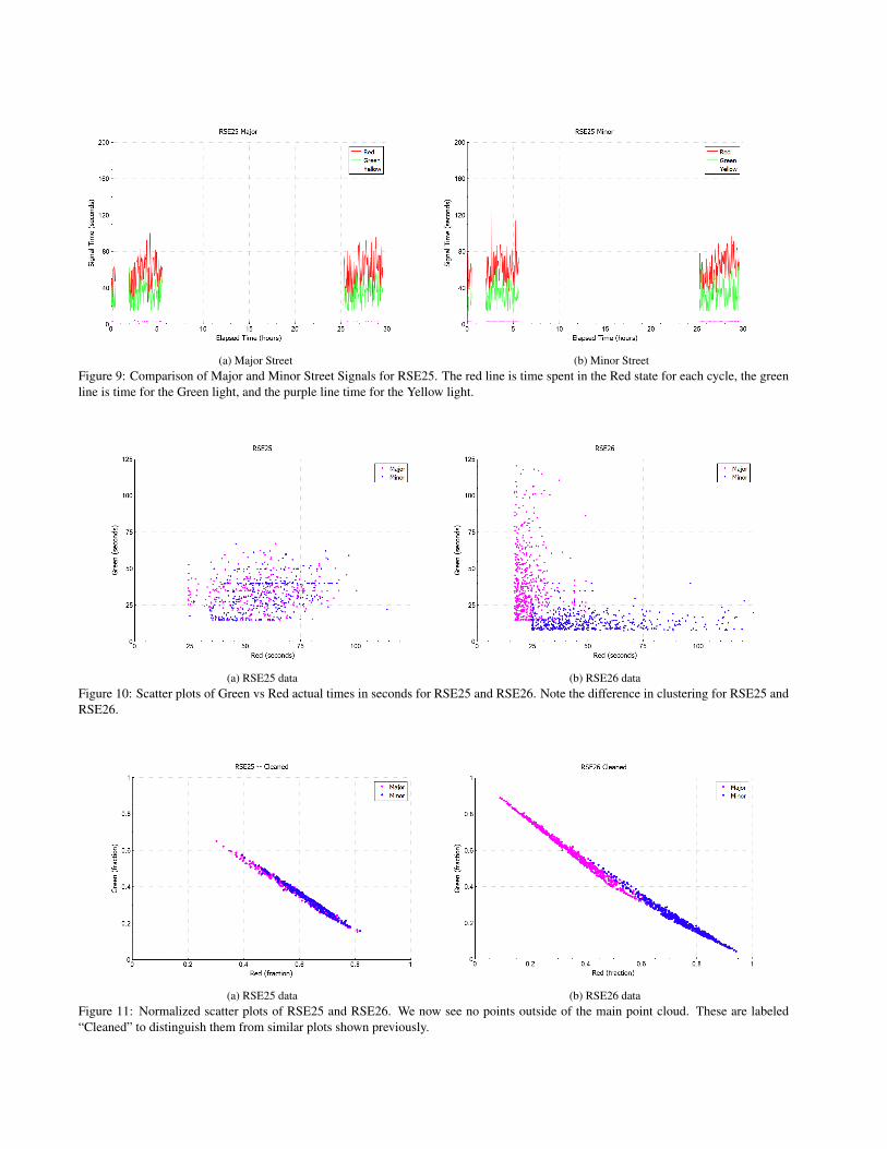
(a) Major Street (b) Minor StreetFigure 9: Comparison of Major and Minor Street Signals for RSE25. The red line is time spent in the Red state for each cycle, the greenline is time for the Green light, and the purple line time for the Yellow light.

(a) RSE25 data (b) RSE26 dataFigure 10: Scatter plots of Green vs Red actual times in seconds for RSE25 and RSE26. Note the difference in clustering for RSE25 andRSE26.

(a) RSE25 data (b) RSE26 dataFigure 11: Normalized scatter plots of RSE25 and RSE26. We now see no points outside of the main point cloud. These are labeled“Cleaned” to distinguish them from similar plots shown previously.

Figure 12: Normalized scatter plots of RSE29 with closeup views(insets) showing a point from the Major road (left) and two pointsfrom the Minor road.

Figure 13: The states of the traffic signals in time on Major andMinor roads. The arrow shows the long Green light that gives thepoint shown in Figure 12 (upper inset).

We see in Figure 15, which shows the states of the signals as timeprogresses, and it is clear we have a very long Red light on theMinor road corresponding to a very long Green light for the Majorroad. This is almost certainly due to vehicles taking priority onthis Major road. This is, in effect, a Signal Data attack.

The apparent slope of the line formed by the changed Redlight data may be explained as follows. The total time (T) is Red+ Green + Yellow and the points plotted are Red/T, Green/T. Ne-glecting the Yellow time Red/(Red+Green) + Green/(Red+Green)= 1. This is a reminder of the equation of a line ax+by = c. Nowwe restrict the Red to values that are nearly equal to yellow so wehave approximately 2Rx+Gy = 1, or, a line with a slope of −2.

We explore the ability to detect a particular Signal Data at-tack by simulating the data pattern expected. In reading the datawe change the state from Red to Green after 4 seconds, limitingthe Red time and lengthening the Green time. In this experimentwe tampered with every third cycle. We call this mutated data.

In Figure 16 we see a detailed examination of points fromthe mutated data and from the original data. Using the meta-data we can see the resulting calculations for the mutated point T= 4.00+70.99+3.9 = 78.89. Red fraction, R f = 4./78.89 = .05,and Green, G f = 70.99/78.89 = 0.899. For the point fromthe unmodified data we see a very long green light time, and

Figure 14: Picture of the raw data file with rows hidden to showthe data that gives point (0.73,0.22) in the Major road data. Leftcolumn is epoch time, the next column is state, 1 = Red, 3 =Green, 4 = Yellow, and then the time in that state. The two rightmost columns are state and time for the Minor road.

Figure 15: The states of the traffic signals in time on Major andMinor roads. The arrow shows the end of the cycle that gives theright most point in Figure 12 (lower inset).

Figure 16: Detailed examination of a point resulting from mutateddata (smaller circle), and a point from the unmodified data (largercircle).

(a) Scatter plot without modifying the data

(b) Red limited to 4 seconds for 90 cycles of Major road.Figure 17: This is the result of mutating the data to shorten theRed light time for the Major road to appear to give priority.

T = 21.96+375.17+3.92 = 401.05, and R f = 21.96/401.05 =0.055, and G f = 385.17/401.05 = 0.94

We return to the scatter plots showing the raw time in sec-onds for the Red and Green states. In Figure 17 we see the resultof forcing the shorter Red light times.

In a similar manner we alter the data in RSE25. This inter-section displays somewhat different characteristics from the oth-ers. The modified cycles are still apparent. We see that the obvi-ous very short Red lights in both cases are easily distinguishablefrom the cluster of points that make up the bulk of the cycles seen.

6 Conclusions and Future WorkIntrusion detection is crucial for maintaining a reliable and

safe traffic control system for our daily life. Different from pre-vious methods, in this work we demonstrate that traffic light datamay be applied to detect intrusion to the traffic control system.To achieve that, we devised a first visual analytics system to helpprocess and analyze a large-scale traffic light data that is madeavailable to the public for the first time. Our system integratesa number of data cleaning operations and summary informationcomputations specifically developed for the traffic light data. Italso provides a few simple but effective visualization and user in-teractions to support a level-of-details data exploration of the traf-fic light data. We have applied the developed system to success-fully identify a number of errors hidden in the given data that are

(a) Scatter plot without modifying the data

(b) Red limited to 4 seconds for 99 cycles of Major roadFigure 18: This is the result of mutating the data to shorten theRed light time for the Major road to appear to give priority. TheGreen light is given the additional time taken from the Red lighttime.

difficult to find otherwise. Our system also effectively revealedthe abnormal behaviors in the given traffic light data (e.g., veryshort or long Red and Green light times) that indicate the poten-tial attacks to the corresponding traffic signal system.

6.1 Summary of ResultsVarious preprocessing calculations and plotting techniques

have revealed subtle errors in the data. We identified two rootcauses of errors: missing data, and records out of order. Both ofthese could reasonably be attributed to Light Control (describedin Section 1) hacking. These more likely have other explana-tions. The data recording may have been turned off overnight.The records out of order may have been caused by the data log-ging software not maintaining the correct sequence when mergingdata from various intersections. We just don’t know the source ofthe errors. When the data errors were removed, we were able tofind such anomalies such as very short and very long Green lights.These may have been caused by manipulation of the system be-yond our research.

6.2 Limitations and Future workThere are a number of limitations of our current approach

that we plan to improve in the future. First, while we believe a

short Green light on the Minor road is caused by the test vehicles,the short Green light on the Major road could possibly be the re-sult of signal tampering. We don’t know the system logic; it mayjust rush the whole cycle to sync with an approaching vehicle.It’s probably reasonable to assume that the points at the extremeedges of the normalized plots are not due to tampering, but tonormal operations. Further investigation is needed to clarify this.

Second, the intersections in this study were simple, i.e., oneMajor road and one Minor road, and there is no “turn lane” signal.A more complex intersection may also be considered. The addi-tional part of the complete cycle when a turn lane is introducedmay be observed for strange behaviors. For example, to facilitatesetting the light Green in time for a particular vehicle’s arrival theGreen light for the turn lane may be skipped altogether.

Third, the current system is developed specifically for a traf-fic light data, which we would like to apply to other data of thistype. It is conceivable that for the purpose of security monitoringa record could be generated at every state transition for the signal.This would reduce the volume of data. With fewer records longertimes could be studied. Once patterns emerge machine learning orother automated methods could be developed to monitor signalsin real time. A “sliding window” of time may be used to monitorthe signal and an alert issued before there is major disruption inthe system.

References[1] Ahn, K.; Rakha, H.;Hale, D. (2015), Multi-Modal Intelligent Traffic

Signal Systems (MMITSS) Impacts Assessment [Online]. Available:https://rosap.ntl.bts.gov/view/dot/3557

[2] Andrienko, G. ;Andrienko, N.;Hurter, C.;Rinzivillo, S.;Wrobel, S.(2011) From movement tracks through events to places: Extractingand characterizing significant places from mobility data,” 2011 IEEEConference on Visual Analytics Science and Technology (VAST),Providence, RI 161-170 2011.

[3] Exposing Congestion Attack on Emerging Connected Vehicle basedTraffic Signal ControlChen, Q.;Yin, Y.;Feng, Y.;Mao, Z.;Liu, H. (2018)Network and Distributed Systems Security (NDSS)Symposium, San Diego, CA, [Online] Available:https://pdfs.semanticscholar.org/2f41/0fd80f5468307647432d95ec5f268ac1db11.pdf

[4] Milnik, j.( 2019) How to build a Google Data Studio Dashboard[online] Available: https://www.socialmediaexaminer.com/how-to-build-google-data-studio-dashboard

[5] Ernst, J.; Michaels, A. (2017) Framework for Evaluatingthe Severity of Cybervulnerability of a Traffic Cabinet Trans-portation Research Record 2619(1), 55–63 [Online] Available:https://doi.org/10.3141/2619-06

[6] Etoty, R; Erbacher, r (2014) A Survey of VisualizationTools Assessed for Anomaly-Based Intrusion DetectionAnalysis Army Research Laboratory [Online] Available:https://apps.dtic.mil/dtic/tr/fulltext/u2/a601590.pdf

[7] N. Ferreira, J. Poco, H. T. Vo, J. Freire and C. T. Silva, (2013) VisualExploration of Big Spatio-Temporal Urban Data: A Study of NewYork City Taxi Trips IEEE Transactions on Visualization and Com-puter Graphics (19)12, 2149-2158, 2013.

[8] Ghena, B.; Beye, W.; Hillaker, A.; Pevarnek, J.; Halderman, J.Green lights forever: Analyzing the Security of Traffic InfrastructureWOOT’14 Proceedings of the 8th USENIX conference on Offensive

Technologies[9] Haussler, J.; Stein, M.; Seebacher, D.; Janetzko, H.;

Schreck, T.; Keim, D. (2018) Visual Analysis of Ur-ban Traffic Data based on High-Resolution and High-Dimensional Environmental Sensor Data Visualization inEnvironmental Sciences (EnvirVis 2018) [Online] Available:https://pdfs.semanticscholar.org/5002/f43e0e85625e3c7afe03b0a3f428b1ded5d9.pdf

[10] Kaur, J. (2016) Data Visualization with GGpplot2 [online] Avail-able: https://datascience899.wordpress.com/category/ggpplot2/

[11] McLendon, M.;Shhead, t.; Wilson, A.;Wylie, B.; Baumes, j. (2010),Network algorithms for information analysis using the Titan Toolkit44th Annual 2010 IEEE International Carnahan Conference on Se-curity Technology (1-10) San Diego, CA

[12] McMillian, R. (2007), Two Charged withhacking LA traffic lights [online], Available:https://www.computerworld.com/article/2549204/two-charged-with-hacking-la-traffic-lights.html 103-111 (2010)

[13] Pack, M;Wongsuphasawat, K (2009) ICE – Visual Analytics forTransportation Incident Datasets 2009 IEEE International Confer-ence on Information Reuse & Integration 200-205 (2009) Las Vegas,NV

[14] Sisense (2019) Power to the Analytics Builders [online] Available:https://www.sisense.com

[15] Tableau (2019) Changing the Way You Think About Data [online]Available: https://www.tableau.com

[16] Tela, A. (2008), Data Visualization Principles and Practice A. K.Peters Ltd

[17] Teoh, S.;Ma, K; Wu, S; Jankun-Kelly, T (2004) Detecting flaws andintruders with visual data analysis IEEE Computer Graphics and Ap-plications

[18] Wang, Z.;Lu, M.;Yuan, X.;Zhang, j.;Wetering, H. (2013) VisualTraffic Jam Analysis Based on Trajectory Data IEEE Transactionson Visualization and Computer Graphics (19)12, 2159-2168, 2013.

[19] Zeng, W.; Fu, C.;Arisona, S.;Erath, A.;Qu, H. Visualizing Mobilityof Public Transportation System IEEE Transactions on Visualizationand Computer Graphics (20) 12, 1833-1842, 2014.

Author BiographyPlease submit a brief biographical sketch of no more than 75 words.

Include relevant professional and educational information as shown in theexample below.

Glenn Turner is a PhD student at the University of Houston De-partment of Computer Science. After a career writing engineering soft-ware, earned a masters degree in Computer Science from the Universityof Houston (December 219) with emphasis on simple system for data vi-sualization.

Guoning Chen is an Associate Professor at the Department of Com-puter Science at the University of Houston. He earned his Ph.D. in Com-puter Science from Oregon State University in 2009. Before joining theUniversity of Houston, he was a post-doctoral research fellow at the Sci-entific Computing and Imaging (SCI) Institute at the University of Utah.His research interests are in Data Visualization, Geometric Modeling, Ge-ometry Processing, and Physically-based Simulations.

Yunpeng Zhang holds a Ph.D. degree in computer science. He isworking as an Assistant Professor at University of Houston. Dr. Zhanghas worked for Boise State University and Dakota State University (U.S.),University of Melbourne (Australia), and Imperial College London (U.K.)as a Cybersecurity and Software Engineering expert for more than 15

years. Dr. Zhang’s research interests include cybersecurity and softwareengineering. He has invented more than 40 high-performance/securitynew algorithms/methods and developed 8 software systems. He has pub-lished 80 papers in peer-reviewed journals and conferences.