Embed Size (px)
Citation preview
A very Practical Guide to Light FrontHolographic QCD
Liping Zou and H.G. Dosch 1
Institute of Modern Physics, Chinese Academy of SciencesLanzhou
The aim of these lectures is to convey a working knowledge of Light Front Holo-graphic QCD and Supersymmetric Light Front Holographic QCD. We first givean overview of holographic QCD in general and then concentrate on the applica-tion of the holographic methods on QCD quantized in the light front form. Weshow how the implementation of the supersymmetric algebra fixes the interactionand how one can obtain hadron mass spectra with the minimal number of pa-rameters. We also treat propagators and compare the holographic approach withother non-perturbative methods. In the last chapter we describe the applicationof Light Front Holographic QCD to electromagnetic form factors.
1permanent address: Institut f. Theoretische Physik der Universitat Heidelberg, Germany.
arX
iv:1
801.
0060
7v1
[he
p-ph
] 2
Jan
201
8
Contents
1 Introduction 4
1.1 Preliminary Remarks . . . . . . . . . . . . . . . . . . . . . . . . . . . . . . . 4
1.2 Old string theory in strong interactions . . . . . . . . . . . . . . . . . . . . . 6
1.3 AdS/CFT . . . . . . . . . . . . . . . . . . . . . . . . . . . . . . . . . . . . . 9
2 Some mathematical preparations 12
2.1 The general claim . . . . . . . . . . . . . . . . . . . . . . . . . . . . . . . . . 12
2.2 Metric in 5-dimensional Anti-de-Sitter space. . . . . . . . . . . . . . . . . . . 13
2.2.1 Euclidean Metric . . . . . . . . . . . . . . . . . . . . . . . . . . . . . 13
2.2.2 Non-Euclidean metric: Anti-de-Sitter space . . . . . . . . . . . . . . 13
2.3 Relation between AdS and CFT parameters . . . . . . . . . . . . . . . . . . 15
2.4 Gauge Theory in the limit Nc →∞ . . . . . . . . . . . . . . . . . . . . . . . 16
3 The AdS action and wave equations for a (pseudo-)scalar and a vectorfield 18
3.1 The (pseudo-)scalar field . . . . . . . . . . . . . . . . . . . . . . . . . . . . . 18
3.1.1 Euclidean metric . . . . . . . . . . . . . . . . . . . . . . . . . . . . . 18
3.1.2 AdS5 metric . . . . . . . . . . . . . . . . . . . . . . . . . . . . . . . 19
3.1.3 Solution and transformation of the equation of motion . . . . . . . . 21
3.2 Modifications of the action: The hard- and soft-wall model . . . . . . . . . . 21
3.2.1 The hard wall model [16, 17] . . . . . . . . . . . . . . . . . . . . . . . 21
3.2.2 The soft wall model [18] . . . . . . . . . . . . . . . . . . . . . . . . . 23
3.3 Vector Field . . . . . . . . . . . . . . . . . . . . . . . . . . . . . . . . . . . 24
4 Light front holographic QCD 27
1
4.1 Wave functions in light front (LF) quantization . . . . . . . . . . . . . . . . 27
4.2 Bound state equations for mesons with arbitrary spin . . . . . . . . . . . . . 30
4.3 Light Front Holographic QCD (LFHQCD) . . . . . . . . . . . . . . . . . . . 31
4.4 Bound state equations for baryons with arbitrary spin . . . . . . . . . . . . 33
4.5 Inclusion of small quark masses . . . . . . . . . . . . . . . . . . . . . . . . . 36
4.6 Summary . . . . . . . . . . . . . . . . . . . . . . . . . . . . . . . . . . . . . 39
5 Supersymmetric light front holographic QCD 40
5.1 Constraints from conformal algebra . . . . . . . . . . . . . . . . . . . . . . . 41
5.2 Constraints from superconformal (graded) algebra . . . . . . . . . . . . . . . 43
5.2.1 Supersymmetric QM . . . . . . . . . . . . . . . . . . . . . . . . . . . 43
5.2.2 Superconformal quantum mechanics . . . . . . . . . . . . . . . . . . . 44
5.2.3 Consequences of the superconformal algebra for dynamics . . . . . . 45
5.2.4 Spin terms and small quark masses . . . . . . . . . . . . . . . . . . . 47
5.2.5 Comparison with experiment . . . . . . . . . . . . . . . . . . . . . . . 47
5.2.6 Completing the supersymmetric multiplet - Tetraquarks . . . . . . . 50
5.3 Implications of supersymmetry on Hadrons containing heavy quarks . . . . 52
5.3.1 The experimental situation . . . . . . . . . . . . . . . . . . . . . . . 52
5.3.2 Linear trajectories . . . . . . . . . . . . . . . . . . . . . . . . . . . . 55
5.3.3 Consequences of heavy quark symmetry (HQS) . . . . . . . . . . . . 60
5.4 Extension to two heavy quarks . . . . . . . . . . . . . . . . . . . . . . . . . . 60
5.4.1 Completing he supermultiplet in the heavy hadron sector . . . . . . 61
5.5 Summary . . . . . . . . . . . . . . . . . . . . . . . . . . . . . . . . . . . . . 63
6 The propagator from AdS 64
6.1 The two point function in Holographic QCD . . . . . . . . . . . . . . . . . . 64
6.1.1 The generating functional . . . . . . . . . . . . . . . . . . . . . . . . 64
6.1.2 The classical action . . . . . . . . . . . . . . . . . . . . . . . . . . . . 65
6.2 Soft wall model . . . . . . . . . . . . . . . . . . . . . . . . . . . . . . . . . . 67
6.2.1 Solutions for soft wall model . . . . . . . . . . . . . . . . . . . . . . . 67
6.2.2 The propagator for the conserved current in the holographic soft wallmodel . . . . . . . . . . . . . . . . . . . . . . . . . . . . . . . . . . . 69
2
6.2.3 Physical relevance of conserved current . . . . . . . . . . . . . . . . 70
6.2.4 Propagators for other currents in LFHQCD . . . . . . . . . . . . . . 71
6.2.5 Asymptotic expansion of the two-point function. Comparison withQCD sum rules. . . . . . . . . . . . . . . . . . . . . . . . . . . . . . 72
6.2.6 The propagator in the hard wall model . . . . . . . . . . . . . . . . . 74
6.3 Summary . . . . . . . . . . . . . . . . . . . . . . . . . . . . . . . . . . . . . 75
7 Form factors in AdS 76
7.1 Form factors . . . . . . . . . . . . . . . . . . . . . . . . . . . . . . . . . . . . 76
7.2 Form factor in HQCD and LFHQCD for a (pseudo-)scalar particle . . . . . 77
7.2.1 The “dressed” electromagnetic field in AdS/CFT . . . . . . . . . . . 77
7.2.2 The scaling twist . . . . . . . . . . . . . . . . . . . . . . . . . . . . . 79
7.2.3 General results . . . . . . . . . . . . . . . . . . . . . . . . . . . . . . 80
7.2.4 Final assumptions and results for the form factor . . . . . . . . . . 80
7.2.5 Comparison of π form factor with experiment . . . . . . . . . . . . . 81
7.2.6 The form factor in the parton model, effective wave functions . . . . 83
7.3 Nucleon Form Factors . . . . . . . . . . . . . . . . . . . . . . . . . . . . . . 84
7.3.1 Form factors for spin 12
fields in AdS/CFT . . . . . . . . . . . . . . . 84
7.3.2 A Simple Light-Front Holographic Model for Nucleon Form Factors . 85
7.4 Summary . . . . . . . . . . . . . . . . . . . . . . . . . . . . . . . . . . . . . 89
A Collection of wave functions 91
A.1 Mesons . . . . . . . . . . . . . . . . . . . . . . . . . . . . . . . . . . . . . . . 91
A.2 Baryons . . . . . . . . . . . . . . . . . . . . . . . . . . . . . . . . . . . . . . 92
A.3 Currents . . . . . . . . . . . . . . . . . . . . . . . . . . . . . . . . . . . . . . 92
3
Chapter 1
Introduction
1.1 Preliminary Remarks
Light Front Holograph QCD [1, 2] is a model theory, which tries to explain non-perturbativefeatures of the quantum field theory for strong interactions, QCD. Like in all realistic quan-tum field theories, also in QCD perturbation theory is the only analytical method to obtainrigorous numerical results. Unfortunately the most interesting questions in particle physics,like the calculation of hadron masses, cannot be solved by perturbation theory. The onlyrigorous method to do that are very elaborate numerical calculations with supercomputers.These calculations are performed in Euclidean space-time and the continuum is approxi-mated by a lattice, a set of discrete points and links between.
In order to get some insight into the structure of the most interesting phenomena, onehas to make specific models and approximations. An especially important approach is thesemiclassical approximation of a quantum field theory. Here the complicated structure ofthe interaction, which notably involves virtual particle creation and annihilation (loops), isapproximated by a potential in a Schrodinger-like quantum mechanical equation. All theresults on the structure of atoms and molecules, which follow in principle from quantumelectrodynamics (QED), are not obtained by calculating complicated Feynman diagrams,but by solving the Schrodinger or Dirac equation with the electromagnetic potentials. Thisdoes not mean that quantum field theory is obsolete, since firstly it is used to derive thepotentials in the Schrodinger equation (in the simplest case by one photon exchange), sec-ondly important constraints on the solutions, like those of the Pauli principle, can only bederived from quantum field theory and finally, quantum field theory is used to improve thesemiclassical results, as is done for instance by the calculation of the Lamb shift in QED.
Light front holographic QCD allows to obtain a semiclassical approximation to QCD. Sincethe quarks which constitute ordinary matter are very light, their mass is only a few MeV,the kinematics is ultra-relativistic. In that case the so called Light Front Quantization isthe easiest way to obtain a semiclassical approximation. In it this form of quantization the
4
commutators of the quantum fields are not defined at equal (ordinary) time, but at equal“light front time”, which is the sum of the ordinary time and one of the space coordinates.
The basis of light front holographic QCD is the ”holographic principle”. It states that certainaspects of a quantum field theory in four space-time dimensions can be obtained as limitingvalues of a five dimensional theory 1. In our case the basis is the Maldacena conjecture [3],which states the equivalence of a five dimensional classical theory with a four dimen-sional quantum field theory. The five dimensional classical theory has a non-Euclideangeometry (the so called Anti-de-Sitter metric), the four dimensional quantum field theory isa quantum gauge theory, like QCD, but it has not Nc = 3 colours, but Nc →∞, it has confor-mal symmetry (that is it has no scale) and furthermore it is supersymmetric, that is to eachfermion field there exist also bosonic fields with properties governed by a “supersymmetry”.Unfortunately this ”superconformal” quantum gauge theory2 with infinitely many coloursis rather remote from QCD. Therefore in Light Front Holographic QCD (LFHQCD) onechooses a “bottom-up” approach, that is one modifies the five dimensional classical theoryin such a way as to obtain from this modified theory and the holographic principle realisticfeatures of hadron physics. This reduces the power to explain structural features of hadronphysics, since just this observed structures are used as input to determine the modificationsof the classical 5-dimensional theory. This shortcoming is removed in supersymmetric lightfront holographic QCD (SuSyLFHQCD), which forms the the main subject of these lectures.Here the implementation [4] of superconformal symmetry on the semiclassical theory fixesthe necessary modifications completely. In this SuSyLFHQCD the number of parameters isjust the one dictated by QCD itself (like in lattice QCD). In the limit of massless quarksone has the universal scale (fixed for instance by one hadron mass), and for massive quarksone has also the quark masses as parameters. It should be noted that the underlying super-symmetry is a symmetry between wave functions of observed mesons and observed baryonsand not a supersymmetry of fields. Therefore no new particles like “squarks” or “gluinos”have to be introduced.
The derivation of semiclassical equations for hadron physics is certainly a big achievementof the holographic principle, but not the only one. The correspondence allows in principleto determine all matrix elements of the quantum field theory by the classical solution of thefive-dimensional theory. Therefore one can also calculate form factors in LFHQCD [5, 6].
A limitation on the accuracy of the numerical results is the limit of infinitely many colours.This limit is well studied in the framework of conventional QCD [7] and leads typically toerrors of the order of 10% of the hadronic scale or around 100 MeV.
Since the aim of this notes is to convey a practical working knowledge as fast as possible,this necessitates many omissions of more subtle points. Also the quoted literature is mostlyconfined to subjects directly related to the material, which is explicitly treated in these notes,
1The name is derived from ”hologram” which is a two dimensional picture which contains the informationof a three dimensional object
2The name AdS/CFT correspondence, frequently used for this holographic approach, comes from theAnti-de-Sitter metric and the Conformal Field Theory.
5
p
p
p
p
'
'11
22
s-channel
t-channel
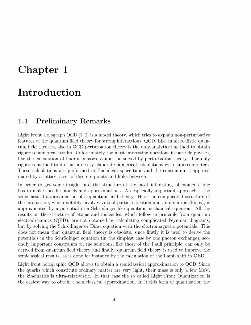
Figure 1.1: Elastic scattering amplitude.
but the quoted literature allows easily to find more sources and to expand the knowledge.
1.2 Old string theory in strong interactions
Before QCD emerged as a consistent theory based on quark and gluon fields in the early1970ies, there was another approach to strong interaction physics, which did not search forelementary particles at all. The basis of this approach was duality. For an elastic scatteringamplitude T (s, t), Fig. 1.1, which depends on the total energy s = (p1 + p2)2 = (p′1 + p′2)2
and the momentum transfer t = (p′1 − p1)2 = (p′2 − p2)2, we have two salient features:1) For low values of s we observe resonances, for instance in N − π scattering the ∆ andhigher resonances. This means that there are poles in the variable s at the resonance masses.The amplitude T (s, t) behaves near the resonance as
T (s, t) ∼ A
s−m2R
For unstable resonances mR has an imaginary part.
2) For high values of s we have Regge behaviour, that is in that limit the amplitude behaveslike
T (s, t) ∼ sα(t),
the function α(t) is called a Regge trajectory.
This gives a good description of high energy scattering, that is for large values of s and fornegative values of t. For positive values of t, which can occur in annihilation, a resonancepole with total angular momentum J occurs at those values of t, where α(t) is a nonnegativeinteger J . It turned out that linear trajectories, that is
α(t) = α0 + α′ · t (1.1)
give a good description of the data. α0 is called the intercept and α′ the slope of thetrajectory. The concept of duality was developed as an attempt to unify these two seeminglyvery different features.
6
-
6
uuuu
uuuuu u
t
J
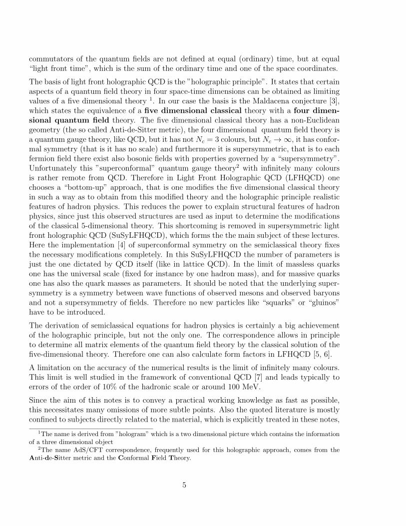
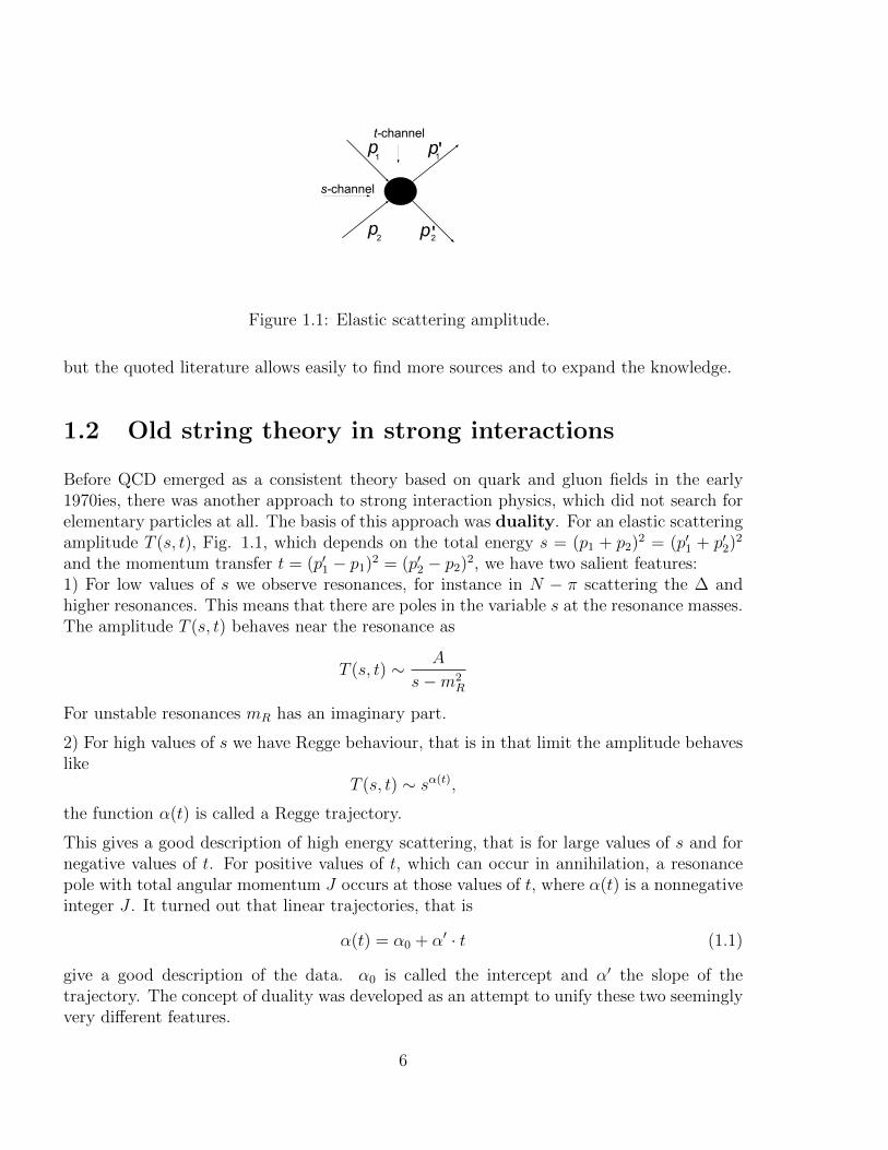
Figure 1.2: Trajectories in the Veneziano model.
rotation vibration
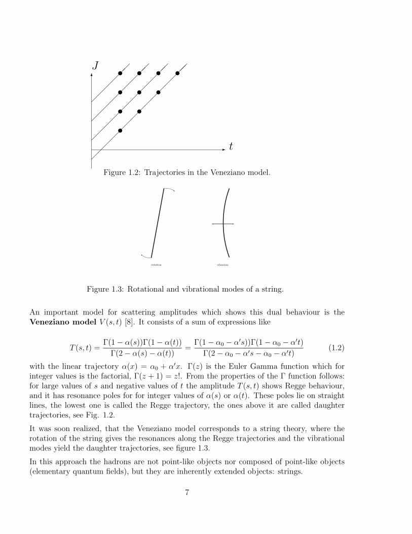
Figure 1.3: Rotational and vibrational modes of a string.
An important model for scattering amplitudes which shows this dual behaviour is theVeneziano model V (s, t) [8]. It consists of a sum of expressions like
T (s, t) =Γ(1− α(s))Γ(1− α(t))
Γ(2− α(s)− α(t))=
Γ(1− α0 − α′s))Γ(1− α0 − α′t)Γ(2− α0 − α′s− α0 − α′t)
(1.2)
with the linear trajectory α(x) = α0 + α′x. Γ(z) is the Euler Gamma function which forinteger values is the factorial, Γ(z + 1) = z!. From the properties of the Γ function follows:for large values of s and negative values of t the amplitude T (s, t) shows Regge behaviour,and it has resonance poles for for integer values of α(s) or α(t). These poles lie on straightlines, the lowest one is called the Regge trajectory, the ones above it are called daughtertrajectories, see Fig. 1.2.
It was soon realized, that the Veneziano model corresponds to a string theory, where therotation of the string gives the resonances along the Regge trajectories and the vibrationalmodes yield the daughter trajectories, see figure 1.3.
In this approach the hadrons are not point-like objects nor composed of point-like objects(elementary quantum fields), but they are inherently extended objects: strings.
7
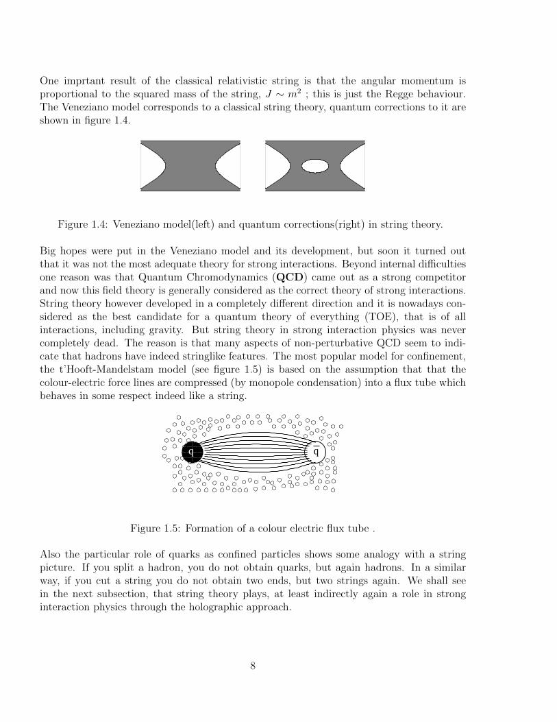
One imprtant result of the classical relativistic string is that the angular momentum isproportional to the squared mass of the string, J ∼ m2 ; this is just the Regge behaviour.The Veneziano model corresponds to a classical string theory, quantum corrections to it areshown in figure 1.4.
Figure 1.4: Veneziano model(left) and quantum corrections(right) in string theory.
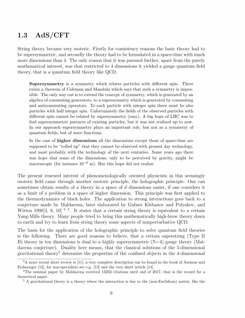
Big hopes were put in the Veneziano model and its development, but soon it turned outthat it was not the most adequate theory for strong interactions. Beyond internal difficultiesone reason was that Quantum Chromodynamics (QCD) came out as a strong competitorand now this field theory is generally considered as the correct theory of strong interactions.String theory however developed in a completely different direction and it is nowadays con-sidered as the best candidate for a quantum theory of everything (TOE), that is of allinteractions, including gravity. But string theory in strong interaction physics was nevercompletely dead. The reason is that many aspects of non-perturbative QCD seem to indi-cate that hadrons have indeed stringlike features. The most popular model for confinement,the t’Hooft-Mandelstam model (see figure 1.5) is based on the assumption that that thecolour-electric force lines are compressed (by monopole condensation) into a flux tube whichbehaves in some respect indeed like a string.
q
Magnetischer Monopol
q
Figure 1.5: Formation of a colour electric flux tube .
Also the particular role of quarks as confined particles shows some analogy with a stringpicture. If you split a hadron, you do not obtain quarks, but again hadrons. In a similarway, if you cut a string you do not obtain two ends, but two strings again. We shall seein the next subsection, that string theory plays, at least indirectly again a role in stronginteraction physics through the holographic approach.
8
1.3 AdS/CFT
String theory became very esoteric. Firstly for consistency reasons the basic theory had tobe supersymmetric, and secondly the theory had to be formulated in a space-time with muchmore dimensions than 4. The only reason that it was pursued further, apart from the purelymathematical interest, was that restricted to 4 dimensions it yielded a gauge quantum fieldtheory, that is a quantum field theory like QCD.
Supersymmetry is a symmetry which relates particles with different spin. Thereexists a theorem of Coleman and Mandula which says that such a symmetry is impos-sible. The only way out is to extend the concept of symmetry, which is generated by analgebra of commuting generators, to a supersymmtry which is generated by commutingand anticommuting operators. To each particle with integer spin there must be alsoparticles with half integer spin. Unfortunately the fields of the observed particles withdifferent spin cannot be related by supersymmetry (susy). A big hope of LHC was tofind supersymmetric partners of existing particles, but it was not realized up to now.In our approach supersymmetry plays an important role, but not as a symmetry ofquantum fields, but of wave functions.
In the case of higher dimensions all the dimensions except those of space-time are
supposed to be “rolled up” that they cannot be observed with present day technology,
and most probably with the technology of the next centuries. Some years ago there
was hope that some of the dimensions, only to be perceived by gravity, might be
macroscopic (for instance 10−6 m). But this hope did not realize.
The present renewed interest of phenomenologically oriented physicists in this seeminglyesoteric field came through another esoteric principle, the holographic principle: One cansometimes obtain results of a theory in a space of d dimensions easier, if one considers itas a limit of a problem in a space of higher dimension. This principle was first applied tothe thermodynamics of black holes. The application to strong interactions goes back to aconjecture made by Maldacena, later elaborated by Gubser Klebanov and Polyakov, andWitten 1998[3, 9, 10] 3 4. It states that a certain string theory is equivalent to a certainYang-Mills theory. Many people tried to bring this mathematically high-brow theory downto earth and try to learn from string theory some aspects of nonperturbative QCD.
The basis for the application of the holographic principle to solve quantum field theoriesis the following. There are good reasons to believe, that a certain superstring (Type IIB) theory in ten dimensions is dual to a highly supersymmetric (N=4) gauge theory (Mal-dacena conjecture). Duality here means, that the classical solutions of the 5-dimensionalgravitational theory5 determine the properties of the confined objects in the 4-dimensional
3A more recent short review is [11], a very complete description can be found in the book of Ammon andErdmenger [12], for non-specialists see e.g. [13] and the very short article [14].
4The seminal paper by Maldacena received 13233 citations until end of 2017, that is the record for atheoretical paper.
5 A gravitational theory is a theory where the interaction is due to the (non-Euclidean) metric, like the
9
field theory. This sounds very promising. The five dimensional gravitational theory is rathersimple, it is based on the metric of a 5-dimensional space, the so called Anti-de-Sitter space,AdS5. The dual quantum field theory is very far from QCD. It is a gauge quantum fieldtheory, but it is a conformal theory that contains no mass scale and therefore cannot giverise to hadrons with finite masses. Furthermore it is supersymmetric and has an infinitenumber of colours.
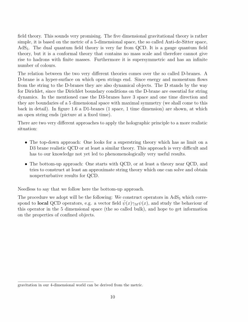
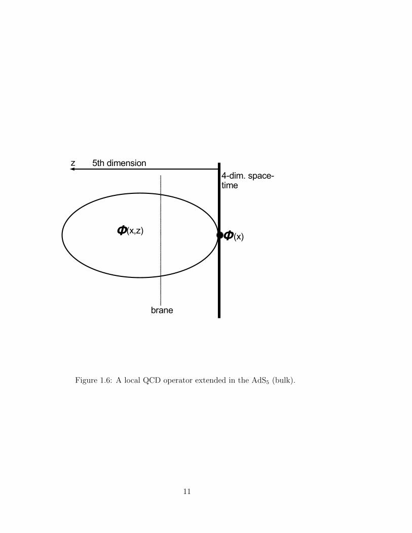
The relation between the two very different theories comes over the so called D-branes. AD-brane is a hyper-surface on which open strings end. Since energy and momentum flowsfrom the string to the D-branes they are also dynamical objects. The D stands by the wayfor Dirichlet, since the Dirichlet boundary conditions on the D-brane are essential for stringdynamics. In the mentioned case the D3-branes have 3 space and one time direction andthey are boundaries of a 5 dimensional space with maximal symmetry (we shall come to thisback in detail). In figure 1.6 a D1-branes (1 space, 1 time dimension) are shown, at whichan open string ends (picture at a fixed time).
There are two very different approaches to apply the holographic principle to a more realisticsituation:
• The top-down approach: One looks for a superstring theory which has as limit on aD3 brane realistic QCD or at least a similar theory. This approach is very difficult andhas to our knowledge not yet led to phenomenologically very useful results.
• The bottom-up approach: One starts with QCD, or at least a theory near QCD, andtries to construct at least an approximate string theory which one can solve and obtainnonperturbative results for QCD.
Needless to say that we follow here the bottom-up approach.
The procedure we adopt will be the following: We construct operators in AdS5 which corre-spond to local QCD operators, e.g. a vector field ψ(x)γMψ(x), and study the behaviour ofthis operator in the 5 dimensional space (the so called bulk), and hope to get informationon the properties of confined objects.
gravitation in our 4-dimensional world can be derived from the metric.
10
5th dimension
ΦΦ
4-dim. space-time
(x)(x,z)
brane
z
Figure 1.6: A local QCD operator extended in the AdS5 (bulk).
11
Chapter 2
Some mathematical preparations
2.1 The general claim
The AdS-CFT correspondence claims, that in a certain limit the essential results of a quan-tum field theory, like propagators, bound state poles etc, can be obtained from the classicalsolutions of the higher dimensional gravitational theory. This can be very concisely formu-lated in terms of the generating functionals. We shall come back to that in more detail inChapt. 6 and give here only a short overview.
A generating functional Z[j] contains all information on the observables of quantum fieldtheory. For a free theory we have Z[j] = e
∫dx dy j(y)D(x−y)j(x), where D(x − y) is the free
propagator.
The correspondence statement claims:
ZFT [j] = iSAdS[Φcl]/Φcl
z→0−→j(2.1)
where Φcl is the solution of the classical equations of motion derived from the action in theAdS5.
We shall exploit that relation in chapter 6 in order to calculate propagators. But here wetake a very practical attitude. We construct in AdS5 the action for a field with the samequantum numbers as the one we want to investigate in the 4-dimensional quantum fieldtheory. The classical equations of motion, the solutions of which minimize the action, arethe bound state wave equations for the hadrons. But before we come to that, we have tomake some preparatory steps.
12
2.2 Metric in 5-dimensional Anti-de-Sitter space.
2.2.1 Euclidean Metric
The line element in Minkowski metric, that is our usual relativistic space time continuum,is given by:
ds2 = −(dx1)2 − (dx2)2 − (dx3)2 + (dx4)2 =4∑
µν=1
ηµν dxµdxν (2.2)
gµν is called the metric tensor. In Minkowski space the metric tensor in Cartesian coordinatesis particularly simple and given by:
ηµν =
−1 0 0 00 −1 0 00 0 −1 00 0 0 1
(2.3)
Since ηµν is not positive definite, it is called a pseudo-Euclidean metric tensor and geometryin Minkowski space is called pseudo-Euclidean.
The metric tensor in a Minkowski space with 3 space, 1 time variable and an additionalspacelike 5th coordinate is
ηMN =
−1 0 0 0 00 −1 0 0 00 0 −1 0 00 0 0 1 00 0 0 0 −1
(2.4)
2.2.2 Non-Euclidean metric: Anti-de-Sitter space
In non-Euclidean geometry, the elements of the metric are no longer constants, but maydiffer from point to point. The line element of (2.2) therefore becomes:
(ds)2 =∑MN
gMN(x) dxM dxN (2.5)
where gMN is a symmetric matrix function, gMN(x) = gNM(x).
The metric tensor in AdS5 is 1 :
gMN =R2
z2
−1 0 0 0 00 −1 0 0 00 0 −1 0 00 0 0 1 00 0 0 0 −1
=R2
z2ηMN (2.6)
1The specific form of the metric depends naturally on the choice of coordinates. In AdS5 we alwayschoose the so called Poincare coordinates
13
Here z = x5 is the fifth variable, normally called the hologtraphic variable, R is a measurefor the curvature of the space.
The modulus of the determinant of the metric tensor is accordingly:
|g| =(R2
z2
)5
(2.7)
The inverse metric tensor is given by upper indices:
gMN−1 ≡ gMN (2.8)
that is∑5
N=1 gMN gNA = δAM , in Euclidean metric one has ηMN = ηMN .
In the future we will use the Einstein convention: over upper and lower indices with equalname will be summed, that is e.g.
gMN gNA ≡
5∑N=1
gMN gNA. (2.9)
One calls lower indices covariant indices and upper indices contravariant indices. With themetric tensor and its inverse one can transform a covariant into a contravariant index andvice versa: aM = gMNaN , aM = gMNa
N .
With the help of the metric tensor we can construct easily invariants from covariant andcontravariant quantities. If aM and bM are covariant vectors in AdS, then the productgMN aM bN is an invariant, like the 4-product of two Lorentz vectors in Minkowski space,ηµνaµ bν , is an invariant.
The invariant volume element in AdS5 is the Euclidean volume element d4xdz multipliedby the square root of the modulus of the determinant of gMN . For the metric tensor (2.6)the determinant is the product of the diagonal elements and hence we obtain as invariantvolume element of AdS5:
dV = d4xdz√|g| = d4x dz
(R
z
)5
(2.10)
where we have inserted the modulus of the determinant of gMN with the relation (2.7).
Since in the following we shall always jump between the 4-dimensional Minkowski space andthe 5-dimensional space AdS5 we will introduce the following conventions:
The Greek indices, µ, ν, α . . . run from 1 to 4, where x4 = c t is the timelike variable. In the5-dimensional space, we shall use capital Latin letter, M,N,A . . . which run from 1 to 5,and x5 = z.
14
2.3 Relation between AdS and CFT parameters
Before coming to the relation, we have to introduce the Planck units. They are named, sincePlank was the first to look for natural units, which are independent of human standards(like meter, second etc) and he realized that with his constant h he could achieve it.
In conventional units we have three dimensionful quantities: mass [m], time [t], and length [l].We have as fundamental constants the velocity of light c, Planck’s constant h, and Newton’sconstant of gravity GN . The natural unit for the velocity is certainly the velocity of light c,the natural unit of Energy is [m] c2, for the action [E][t] the natural unit is h. Therefore wecan reduce the three dimensions to only one, e.g. the length. We have [t] = [l]/c; [m] = h
c[l].
The gravitational constant is defined in Newton’s law: F = m1m2
r2GN . With that we can
obtain as natural unit for the remaining dimension, the length, the Planck length:
lP =
√h
c3Gn ≈ 1.6× 10⁻³³cm (2.11)
The natural unit for the mass and the time are the Planck mass mP and the Planck timetP :
mP =
√hc
GN
≈ 1.2× 10¹⁴GeV/c2 ≈ 2.2× 10⁻⁵g (2.12)
tP =lPc≈ 5.4× 10−44s (2.13)
From string theory one deduces the following relation between rhe AdS5 and CFT quantities:lPR
AdS
=
√π
21/8N1/4c
≈ 1.6
N1/4c
CFT
(2.14)
In a gravitational theory quantum effects can be neglected if lP R. In our universe, wherethe curvature radius is infinity or very large and the Planck length is tiny, quantum effectsare completely negligible. But in the very early universe, say one Planck time tP after thebig bang, quantum gravity must have played a crucial role, therefore we cannot say anythingabout the big bang properly.
But back to AdS, in order to treat gravity in AdS as a classical theory, the number of coloursmust be huge (> 104), so the application in our world, where the gauge theory QCD hasthree colours, NC = 3, seems to be hopeless. But fortunately gouge theories with NC →∞are well studied and might give results not so far from N = 3, typical deviations may be1/N2
c ≈ 0.11. We come to this important point in the next subsection.
15
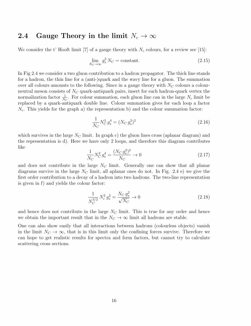
2.4 Gauge Theory in the limit Nc →∞We consider the t’ Hooft limit [7] of a gauge theory with Nc colours, for a review see [15]:
limNC→∞
g2s NC = constant. (2.15)
In Fig 2.4 we consider a two gluon contribution to a hadron propagator. The thick line standsfor a hadron, the thin line for a (anti-)quark and the wavy line for a gluon. The summationover all colours amounts to the following. Since in a gauge theory with NC colours a colour-neutral meson consists of NC quark-antiquark pairs, insert for each hadron-quark vertex thenormalization factor 1
NC. For colour summation, each gluon line can in the large Nc limit be
replaced by a quark-antiquark double line. Colour summation gives for each loop a factorNc. This yields for the graph a) the representation b) and the colour summation factor:
1
NC
N3C g
4s = (NC g
2s)
2 (2.16)
which survives in the large NC limit. In graph c) the gluon lines cross (aplanar diagram) andthe representation is d). Here we have only 2 loops, and therefore this diagram contributeslike
1
NC
N2C g
4s =
(NC g2s)
2
NC
→ 0 (2.17)
and does not contribute in the large NC limit. Generally one can show that all planardiagrams survive in the large NC limit, all aplanar ones do not. In Fig. 2.4 e) we give thefirst order contribution to a decay of a hadron into two hadrons. The two-line representationis given in f) and yields the colour factor:
1
N3/2C
N2c g
2s =
NC g2s√
NC
→ 0 (2.18)
and hence does not contribute in the large NC limit. This is true for any order and hencewe obtain the important result that in the NC →∞ limit all hadrons are stable.
One can also show easily that all interactions between hadrons (colourless objects) vanishin the limit NC → ∞, that is in this limit only the confining forces survive. Therefore wecan hope to get realistic results for spectra and form factors, but cannot try to calculatescattering cross sections.
16
gsgs
gsgs
(a)
gsgs
gsgs
(c)
N N N
N N
1√N
1√N
1√N
1√N
(b)
(d)
gs
gs
(e)
N
N
(f)
1√N
1√N
1√N
Figure 2.1: Evaluation of the colour factor for several diagrams. In the diagrams (a) and(c) we have a factor g4
s from gluon exchange. According to (b), where gluon lines have beenreplaced by double lines of quarks, we have 3 loops and hence a factor N3
c . Together withthe normalization factors this yields the overall colour expression 1
NCN3C g
4s which is finite in
the t’Hooft limit (2.15). For the aplanar diagram (c) we have only two loops, see (d) andtherefore the contribution vanishes in the Nc →∞ limit. In the decay diagram (c) we haveg2s , two loops and three vertices. This yields the overall factor 1
N3/2c
N2c g
2s which vanishes in
the t’Hooft limit.
17
Chapter 3
The AdS action and wave equationsfor a (pseudo-)scalar and a vector field
3.1 The (pseudo-)scalar field
3.1.1 Euclidean metric
As mentioned, we can derive all the properties of the 4-dimensional quantum field theory fromthe solutions of the classical action of the higher dimensional theory with a non-Euclideanmetric. Therefore we construct now the AdS action for a (pseudo-)scalar field Φ(x) =Φ(~x, ct, z).
We start with a more familiar case, the action of a free scalar field in Minkoswski space. Itis given by the integral over the Lagrangian L:
A =
∫d4x
1
2(ηνρ ∂νΦ ∂ρΦ− µ2 Φ2)︸ ︷︷ ︸
L
(3.1)
The solutions of the classical equations of motion are the functions Φ(x) for which theaction is minimal. From this follows that the equations of motion for classical fields are theEuler-Lagrange equations:
∂ν∂L
∂(∂νΦ)− ∂L∂φ
= 0. (3.2)
This leads to the wave equation for a free (pseudo-)scalar field, called the Klein-Gordonequation:
ηνρ∂ν∂ρΦ + µ2Φ = 0. (3.3)
18
3.1.2 AdS5 metric
If we go from Euclidean metric to the non-Euclidean AdS5 metric we have in the action (3.1)to replace:
• ηµν → gMN
• d4x→ d4x√|g| dz, see (2.10)
• In principle we have also to replace the normal (Euclidean) derivative ∂µ by the socalled covariant derivative Dµ in AdS5, but for a scalar field the covariant derivative isequal to the the normal one 1
Instead of the action Euclidean (3.1) we obtain in AdS5 geometry:
A =
∫d4x dz
√|g|1
2(gMN ∂MΦ∂NΦ− µ2Φ2)︸ ︷︷ ︸
L
(3.4)
and from (3.2) we obtain instead of the Euclidean equations of motion (3.3) the equationsin non-Euclidean metric:
∂R
(√|g|gRN∂NΦ
)+√|g|µ2Φ = 0. (3.5)
or
gRN(∂R∂NΦ
)+ µ2Φ =
−1√|g|
∂R(√|g|gRN
)∂NΦ (3.6)
We see that the interaction in the non-Euclidean metric leads to an interaction term namelythe r.h.s. of (3.6), this is due to the term ∂R
(√|g|gRN
)∂NΦ. If the metric is Euclidean,
the elements of the metric tensor are independent of the coordinates and the r.h.s of (3.6)vanishes in that case.
In AdS5 we have, see sect. 2.2.2
gAB =R2
z2ηAB gAB−1 = gAB =
z2
R2ηAB |g| =
(R2
z2
)5
(3.7)
therefore the l.h.s. of (3.6) depends only on the holographic variable x5 = z.
It is convenient for further calculations to write
R2
z2≡ e2A(z) with A(z) = − log z + logR (3.8)
1 Since the displacement of a vector or a tensor in non-Euclidean geometry depends on the metric, thishas also to be considered in the derivative. The covariant derivative DM of a vector field VN (x) contains theso called Christoffel symbol ΓK
MN : DM VN (x) = ∂MVN − ΓKMN VK , the Christoffel symbol can be calculated
from the metric tensor gMN (x), see e.g. [2], App. A.
19
Then we have
gMN = e2A(z)ηMN ; gMN = e−2A(z)ηMN√|g| = e5A(z) (3.9)
and obtain
L =1
2e5A(z)
(e−2A(z)ηMN∂MΦ ∂NΦ− µ2Φ2
)(3.10)
=1
2eκA(z)
(ηMN∂MΦ ∂NΦ− e2A(z)µ2Φ2
)(3.11)
with κ = 3.
The ingredients of the Euler-Lagrange equations
∂A∂L
∂(∂AΦ)− ∂L∂Φ
= 0 (3.12)
are
∂A∂L
∂(∂AΦ)= ∂A
(eκA(z)ηAB∂BΦ
);
∂L∂Φ
= −µ2Φe(κ+2)A(z); κ = 3 (3.13)
From that we obtain the wave equation for the (pseudo)scalar field in AdS5:
eκA(z)
(ηαβ∂α∂βΦ− ∂2
zΦ− κ∂zA(z)∂zφ+ µ2e2A(z)Φ
)= 0. (3.14)
where according to the convention of sect. 2.2.2 the indices α, β run from 1 to 4 (Minkowskispace).
For most cases it is convenient to work with the transformed field Φ(q, z) where theMinkowski coordinates of the field Φ(x, z) are Fourier transformed.
Φ(x, z) =
∫d4q
(2π)4eiqx Φ(q, z) (3.15)
Then we can replaceηαβ∂α∂βΦ(x, z)→ −q2 Φ(q, z)
and obtain for Φ(q, z) the equation(−∂2
z −(κ∂zA(z)
)∂z − q2 +
(µR)2
z2
)Φ(q, z) = 0 (3.16)
inserting (3.8) we arrive finally at the wave equation(−∂2
z +κ
z∂z +
(µR)2
z2− q2
)Φ(q, z) = 0 (3.17)
with κ = 3.
20
3.1.3 Solution and transformation of the equation of motion
The general solution of the differential equation (3.17) can be obtained with the mathematicaprogram:
Φ(q, z) = (qz)(1+κ)/2(AJν(qz) +B Yν(qz)
)with ν =
√(µR)2 + (κ+ 1)2/4 (3.18)
Mathematica: ”BesselJ[n, z] gives the Bessel function of the first kind J(n, z).”,”BesselY[n, z] gives the Bessel function of the second kind Y (n, z).”
The general solution Φ(q, z) of (3.17) is therefore:
Φ(q, z) = Az2 Jν(qz) +B z2 Yν(qz) with ν2 = (µR)2 + 4 (3.19)
In the next few chapters we shall only consider the solution which is regular at z = 0, thatis we put B = 0. We can transform (3.17) also into a Schrodinger-like equation by rescaling,we introduce ΦS(q, z):
Φ(q, z) = z3/2ΦS(q, z) (3.20)
then the linear derivative in (3.17) vanishes and we obtain:(−∂2
z +(4µR)2 + 15
4z2
)ΦS(q, z) = q2ΦS(q, z) (3.21)
This looks like a Schrodinger equation with a potential; but this potential does not lead tothe formation of bound states.
We note the disappointing fact, that there are indeed nontrivial solutions to the equationof motion (3.17) or (3.21) , but there is no sign of confinement, since for any value of q2 wefind a solution. This is, however, not astonishing. The AdS5 has what is called maximalsymmetry and this results in conformal symmetry in the corresponding quantum field theoryin the 4-dimensional Minkowski space. We shall come to conformal symmetry later, hereit is sufficient to say that conformal symmetry demands, that there is no mass scale in thetheory. This applies also for classical QCD in the limit of massless quarks, but not to thequantized QCD. Here we have indeed scales (e.g. the nucleon mass).
3.2 Modifications of the action: The hard- and soft-
wall model
3.2.1 The hard wall model [16, 17]
A way to impose the existence of discrete solutions is the hard wall model. Here it is assumed,that the Lagrangian L in 3.4 is only valid for values of z ≤ z0 (so to speak inside a hard
21
5 10 15 20
-0.4
-0.2
0.2
0.4
0.6
0.8
1
j01
6
j02
6
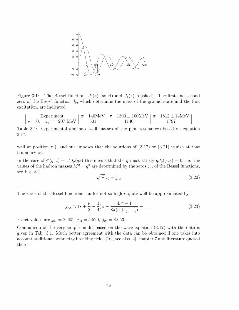
Figure 3.1: The Bessel functions J0(z) (solid) and J1(z) (dashed). The first and secondzero of the Bessel function J0, which determine the mass of the ground state and the firstexcitation, are indicated.
Experiment π 140MeV π 1300± 100MeV π 1812± 14MeVν = 0; z−1
0 = 207 MeV 501 1140 1797
Table 3.1: Experimental and hard-wall masses of the pion resonances based on equation3.17.
wall at position z0), and one imposes that the solutions of (3.17) or (3.21) vanish at thatboundary z0.
In the case of Φ(q, z) = z2Jν(qz) this means that the q must satisfy qJν(q z0) = 0, i.e. thevalues of the hadron masses M2 = q2 are determined by the zeros jνs of the Bessel functions,see Fig. 3.1 √
q2 z0 = jνs (3.22)
.
The zeros of the Bessel functions can for not so high ν quite well be approximated by
jν,s ≈ (s+ν
2− 1
4)π − 4ν2 − 1
8π(s+ ν2− 1
4)− . . . . (3.23)
Exact values are j01 = 2.405, j02 = 5.520, j03 = 8.653.
Comparison of the very simple model based on the wave equation (3.17) with the data isgiven in Tab. 3.1. Much better agreement with the data can be obtained if one takes intoaccount additional symmetry breaking fields [16], see also [2], chapter 7 and literature quotedthere.
22
3.2.2 The soft wall model [18]
In this model a scale is introduced by multiplying the Lagrangian (3.11) with a Dilaton termeϕ(z). This yields the new Lagrangian (κ = 3)
L =1
2eκA(z)+ϕ(z)
(ηMN∂MΦ ∂NΦ− e2A(z)µ2Φ2
)(3.24)
and the Euler Lagrange equation becomes, see (3.14)
eκA(z)+φ(z)
(ηαβ∂α∂βΦ− ∂2
zΦ−(κ∂zA(z) + ∂zϕ(z)
)∂zΦ +
(µR)2
z2Φ
)= 0. (3.25)
The most popular choice for the dilaton term is:
ϕ(z) = λz2 (3.26)
After Fourier transformation, see (3.15) we obtain(− q2 − ∂2
z +(κz− 2λ z
)∂z +
(µR)2
z2
)Φ(q, z) = 0. (3.27)
Here the programm mathematica gives no useful solution and we better transform the equa-tion into a more useful form. With the rescaling
Φ(q, z) = z(κ+1)/2e−λz2/2ΦN(q, z) (3.28)
we obtain
(− ∂2
z −1
z∂z +
L2AdS
z2+ λ2z2 − (κ− 1)λ
)ΦN(q, z) = q2 ΦN(q, z) (3.29)
withL2AdS = (κ+ 1)2/4 + (µR)2. (3.30)
As is shown below this differential equation is closely related to the harmonic oscillator waveequation and has normalized eigenstates with eigenvalues
q2 = M2nL = (4n+ 2LAdS + 2)|λ| − (κ− 1)λ (3.31)
and the eigenfunction for the eigenvalue specified by LAdS and n is
ΦN,nLAdS(z) = zLAdS e−|λ|z2/2 LLAdSn (|λ|z2) (3.32)
where LLn(x) are the associated Laguerre polynomials. In mathematica: LaguerreL[n,x];examples are : LL0 (x) = 1, LL1 (x) = 1 + Lx.
For the solution of (3.27) we obtain, according to (3.28)
ΦnLAdS(z) = z(κ+1)/2 e−λz2
ΦN,nLAdS(z) = zLAdS+(κ+1)/2 e−(|λ|+λ)z2/2 LLAdSn (|λ|z2) (3.33)
23
Derivation of (3.32)-(3.33): The differential operator(− ∂2
z −1
z∂z +
L2
z2+ λ2z2
)= 2Hho (3.34)
is twice the radial differential operator for a two dimensional harmonic oscillator withangular momentum L.
The the eigenvalues areHhoΦnL(q, z) = EnLΦnL (3.35)
withEnL = (2n+ L+ 1)|λ| (3.36)
where L is the angular momentum and n is the radial excitation number. Hence weobtain for the spectrum of the eigenvalues of (3.29) as q2 = 2EnL − (κ − 1)λ and theeigenfunctions are directly those of the 2 dimensional harmonic oscillator.
For the scalar field we have κ = 3 and with L = 0 we thus obtain :
M2n = (4n+ 2)|λ| − 2λ (3.37)
With λ > 0 the lowest (pseudo)scalar particle has mass 0, which is indeed the expected valuein the limit of massless quarks (chiral limit).
By rescalingΦ(q, z) = zκ/2e−ϕ(z)/2φ(q, z) (3.38)
we obtain the Schrodinger-like form(− ∂2
z +4L2
AdS − 1
4z2+ λ2z2 − (κ− 1)λ
)φ(q, z) = q2φ(q, z) (3.39)
where L2AdS = (κ+ 1)2/4 + (µR)2.
3.3 Vector Field
Here we proceed similarly as in electrodynamics in 4 space-time dimensions. We start froma vector field AM , corresponding to the electromagnetic potential and construct the tensorfield
FMN = ∂MAN − ∂NAM (3.40)
which corresponds to the electromagnetic field tensor.
We can use the normal derivatives, since the additional contributions due to the non-Euclidean metric vanish due to the antisymmetric construction. We start from the La-grangian
L =√|g|(1
4gMM ′ gNN
′FMN FM ′N ′ − 1
2µ2 gMM ′AM AM ′
)(3.41)
=R
z
(1
4ηMM ′ ηNN
′FMN FM ′N ′ −
(R
z
)2µ2
2ηMM ′AMAM ′
)(3.42)
24
In contrast to electrodynamics we have added a mass term which breaks gauge invariance inthe AdS5. (This is a so called Proca-Lagrangian). For the soft wall model this Lagrangianis multiplied by a factor eϕ(z) and thus our starting point is the Lagrangian:
L = eA(z)+ϕ(z)
(1
4ηMM ′ ηNN
′FMN FM ′N ′ −
µ2R2
2z2ηMM ′AMAM ′
)(3.43)
where, as in (3.8)
A(z) = − log z + logR and
ϕ(x) =
0 for the hard wall modelλ2z2 for the soft wall model (3.44)
In a gauge theory the 5-mass µ = 0.
The 5 equations of motion are:
∂K∂
∂(∂KAL)L =
δLδAL
, L = 1, · · · 5 (3.45)
From the expression
∂
∂(∂KAL)L = eA(z)+ϕ(z)ηMKηNL(∂MAN − ∂NAM) (3.46)
we obtain the Euler-Lagrange equations:
∂K∂
∂(∂KAL)L − δL
δAL(3.47)
= eA(z)+ϕ(z)
(δ5K(∂zA+ ∂zϕ)ηMKηNL(∂MAN − ∂NAM)
+ηMKηNL(∂K∂MAN − ∂K∂NAM) +(µR)2
z2ηLL
′AL′
)= eA(z)+ϕ(z)
((∂zA+ ∂zϕ)ηM5ηNL(∂MAN − ∂NAM)
+ηMKηNL(∂K∂MAN − ∂K∂NAM) +(µR)2
z2ηLL
′AL′
)(3.48)
Since we have in Minkowski space three vector particles (spin components) and 5 componentsof the potential AK , we can eliminate two components. We choose
A5 = 0 and ηMK∂KAM = 0 (Lorenz gauge) (3.49)
This simplifies (3.48) to:
∂K∂
∂(∂KAL)L = eA(z)−ϕ(z)
((∂zA+ ∂zϕ)ηM5ηNL∂5AN + ηMKηNL∂K∂MAN
)(3.50)
25
from which we obtain in our notation, where Greek indices run from 1 to 4 and ∂5 ≡ ∂z:
ηνλ(ηµκ∂µ∂κAν − ∂2
zAν − (∂zA+ ∂zϕ)∂zAν +(µR)2
z2Aν
)= 0 (3.51)
We make the ansatz for the Fourier transform
Aλ(q, z) = ελ(q)Φ(q, z) (3.52)
where ε(q) is the polarization vector of a transverse vector field, i.e. ε · q = 0, and we obtainfor Φ(z) the wave equation:
(− ∂2
z − (κ∂zA+ ∂zϕ)∂z +(µR)2
z2
)Φ(q, z) = q2Φ(q, z) (3.53)
For the hard wall model we have ϕ = 0, that is (3.53) is like (3.17) with κ = 1. For the softwall model we have ϕ(z) = λ z2, that is (3.53) is like (3.27) with κ = 1.
We can use equations (3.1) and (3.29) − (3.39) also for the vector field, just using for κ thevalue κ = 1, notably we have for the vector particle
L2AdS = (µR)2 + 1. (3.54)
26
Chapter 4
Light front holographic QCD
Before we proceed further in the holographic appoach, we shortly present the kinematicalscheme, which is most adequate for a relativistic semiclassical treatment of a quantum fieldtheory, the Light Front Quantization.
4.1 Wave functions in light front (LF) quantization
There are several schemes on which one can formulate the quantization rules. The most usualis the instantaneous one, which is based on correlators at the same time x4. The light front(LF) quantization [19] is based on quantization rules at equal light front time x+ = x4 + x3.For a review of applications in QCD see e.g. [20]. In the limit of the 3-component of thehadron going to infinity the usual frame based on equal time quantization approaches thelight front quantization frame.
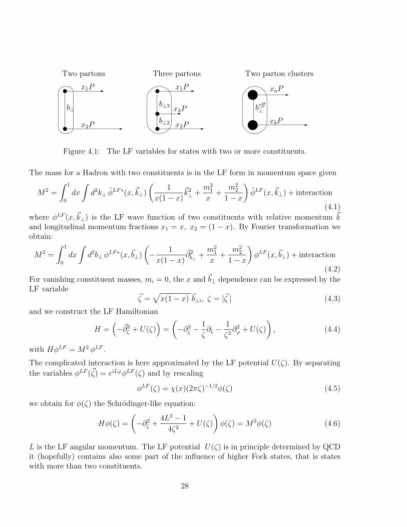
In light front quantization we have the variables x+ = x4+x3, x− = x4−x3 and ~x⊥ = (x1, x2).A wave function in transverse position space with two constituents depends on the thefollowing three variables, see also Fig. 4.1:• The longitudinal momentum fractions of the constituents 1, xi, with
∑i xi = 1. If the
longitudinal momentum of the hadron is P , the longitudinal momentum of the constituenti is xi P .• The two dimensional vector of transverse separation of the two constituents,~b⊥ = x
(1)⊥ −x
(2)⊥
or, in polar coordinates, on b⊥ = |~b⊥| and the polar angle θ. The LF angular momentum Lis given by L = i ∂
∂θ
1The notation xi for the longitudinal momentum fraction is commonly used, it is not to be confused withthe space-time coordinates.
27
Two partons
u
u
-
-
x2P
x1P
b⊥
Three partons#
"
!u
uu
-
-
-
x2P
x3P
x1P
b⊥2
b⊥3
Two parton clusters#
"
!~~
-
-
xbP
xaP
beff⊥
Figure 4.1: The LF variables for states with two or more constituents.
The mass for a Hadron with two constituents is in the LF form in momentum space given
M2 =
∫ 1
0
dx
∫d2k⊥ φ
LF∗(x,~k⊥)
(1
x(1− x)~k2⊥ +
m21
x+
m22
1− x
)φLF (x,~k⊥) + interaction
(4.1)
where φLF (x,~k⊥) is the LF wave function of two constituents with relative momentum ~kand longitudinal momentum fractions x1 = x, x2 = (1 − x). By Fourier transformation weobtain:
M2 =
∫ 1
0
dx
∫d2b⊥ φ
LF∗(x,~b⊥)
(− 1
x(1− x)~∂2b⊥ +
m21
x+
m22
1− x
)φLF (x,~b⊥) + interaction
(4.2)
For vanishing constituent masses, mi = 0, the x and ~b⊥ dependence can be expressed by theLF variable
~ζ =√x(1− x) ~b⊥i, ζ = |~ζ | (4.3)
and we construct the LF Hamiltonian
H =(−~∂2
ζ + U(ζ))
=
(−∂2
ζ −1
ζ∂ζ −
1
ζ2∂2ϕ + U(ζ)
), (4.4)
with HφLF = M2 φLF .
The complicated interaction is here approximated by the LF potential U(ζ). By separating
the variables φLF (~ζ) = eiLϕφLF (ζ) and by rescaling
φLF (ζ) = χ(x)(2πζ)−1/2φ(ζ) (4.5)
we obtain for φ(ζ) the Schrodinger-like equation:
Hφ(ζ) =
(−∂2
ζ +4L2 − 1
4ζ2+ U(ζ)
)φ(ζ) = M2φ(ζ) (4.6)
L is the LF angular momentum. The LF potential U(ζ) is in principle determined by QCDit (hopefully) contains also some part of the influence of higher Fock states, that is stateswith more than two constituents.
28
In the following we shall mainly work with this form (4.24) , but we should keep in mindthat the LF wave function is obtained from the solution φ(ζ) of the Schrodinger like equation(4.6) by dividing through
√ζ.
We obtain an expression for the up to now arbitrary function χ(x) by the normalizationconditions of the two wave functions. If we normalize φ(ζ), the solution of (4.6) by∫
dz|φ(z)|2 = 1 (4.7)
and the LF wave function φLF by∫ ∞0
dx
∫d2b⊥|φLF [x, b⊥]|2 = 1 (4.8)
Then we get the relation
φLF (x, b⊥) =
√x(1− x)
2πζφ(ζ). (4.9)
More than two constituents Since in the holographic correspondence there is only onevariable to describe the internal structure of hadrons, namely the coordinate of the 5thdimension, hadrons with more than two constituents have to be treated as consisting ofclusters. In that case one introduces the effective longitudinal momentum fraction of acluster a:
xaeff =
Na∑i=1
xi, (4.10)
where Na is the number of constituents in the cluster a, and correspondingly one introduceseffective transverse and longitudinal coordinates:
~beff⊥,a = (
Na∑i=1
xi~b⊥,i)/xaeff , ζ =
√xaeff xbeff |~beff
⊥,b −~beff⊥,a|. (4.11)
There is no theoretical limit for Na. For the nucleon with three constituents we have:~beff⊥,d = (x2
~b⊥,2 + x3~b⊥,3)/(x2 + x3), ζeff =
√(x2 + x3)x1
~beff⊥,d =
√x1
x2+x3(x2
~b⊥,2 + x3~b⊥,3).
The introduction of a cluster is purely kinematical and necessary in order to apply the theholographic approach to hadrons with more than two constituents, since there is only onevariable – the holographic variable of the fifth dimension – which describes the internalstructure. This identification does not imply that the cluster is a tightly bound system; itonly requires that essential dynamical features can be described in terms of the holographicvariable. This assumption is supported by the observed similarity between the baryon andmeson spectra.
29
The cluster occurring in this approach cannot be considered as a dynamical diquark and ourapproach is essentially different from a dynamical diquark picture. In the chiral limit thecluster does not acquire a finite mass, since the nucleon and delta masses are described wellby the model without any additional mass terms in the supersymmetric LF Hamiltonian.
In Light Front Holographic QCD (LFHQCD) one identifies the holographic variable z withthe LF variable ζ introduced above. The equal form of the LF Hamiltonian and the boundstate operators (4.1) and (4.6) with the LF Hamiltonian of a two particle (two cluster)state with LF angular momentum L makes it suggestive, to identify the holographic variablex5 = z with the LF variable ζ. The purely formal quantity LAdS =
√(κ+ 1)2/4 + (µR)2
of AdS/CFT becomes then a physical quantity related to the AdS-mass µ, we shall discussthis in detail in sect. 4.3.
4.2 Bound state equations for mesons with arbitrary
spin
For spin higher than 1 the situation becomes very involved, since now we have to use covariantderivatives. A field with spin J > 1 is a symmetric tensor of rank J , ΦN1...NJ . An invariantaction, modified by a dilaton term eϕ(z) is
Seff =
∫ddx dz
√g eϕ(z) gN1N ′1 · · · gNJN ′J
(gMM ′DMΦ∗N1...NJ
DM ′ΦN ′1...N′J
−µ2eff (z) Φ∗N1...NJ
ΦN ′1...N′J
). (4.12)
Here one has to take into account that in non-Euclidean geometry the shift of a tensor isnot only a shift in the variables but generally also mixes the components of the tensor seesect. 3.1.2, footnote 1. Therefore one has to use covariant derivatives and due to these theLagrangian is very complicated and we refer to [21] for details. Here we only quote theresulting bound state equations for mesons with angular momentum L and total spin J .
We Fourier transform the field and extract a z-independent polarization vector εν1...νJ :
Φν1...νJ (q, z) = εν1...νJ ΦL,J(q, z) (4.13)
This leads to the equation of motion:(− q2 − ∂2
z +
(3− 2J
z− ∂zϕ
)∂z +
(µR)2
z2
)ΦL,J(q, z) = 0 (4.14)
Comparing this equation with (3.27) we see that we can use the solutions obtained in sect.3.2.2 by inserting κ = 3− 2J . This leads to:
L2AdS = (J − 2)2 + (µR)2 (4.15)
30
We bring (4.14) into a Schrodinger like form by rescaling
φ(q2, z) = z(2J−3)/2 eϕ(z)/2ΦL,J(q, z) (4.16)
and obtain: (− q2 − ∂2
z +4L2
AdS − 1
4z2+ UAdS(z)
)φ(q, z) = 0 (4.17)
with
UADS(z) =1
4(∂zϕ)2 +
1
2∂2zϕ+
2J − 3
2z∂zϕ (4.18)
For the choice ϕ(z) = λ z2 this simplifies to
UADS(z) = λ2z2 + 2(J − 1)λ (4.19)
Equation (4.17) has normalizable eigenfunctions φnLAdS(z) for the discrete values
q2 = M2nLAdSJ
= (4n+ 2LAdS + 2)|λ|+ 2(J − 1)λ (4.20)
with eigenfunctions
φnLAdS(z) = 1/N zLAdS+1/2LLAdSn (|λ|z2)e−|λ|z2/2 with N =
√(n+ L)!
2n!|λ|−(L+1)/2 (4.21)
They are normalized to∫∞
0dz (φnLAdS(z))2 = 1
The solution for the equation (4.14) of the unmodified field Φ is, see (4.16),
ΦnLAdS(z) =1
Nz2+LAdS−JL(LAdS)
n (|λ|z2)e−(|λ|+λ)z2/2 (4.22)
it is normalized as: ∫ ∞0
dz eλz2
z2J−3ΦnLAdS(z)2 = 1 (4.23)
4.3 Light Front Holographic QCD (LFHQCD)
We compare the soft wall result (4.17) with the general LF Hamiltonian:
Hφ(z) =
(−∂2
ζ +4L2 − 1
4ζ2+ U(ζ)
)φ(z) = M2φ(z) (4.24)
where the LF potential U(ζ) is not determined, and we see the structural identity, if weidentify the holographic variable x5 = z with the LF variable ζ and the AdS quantityLAdS =
√(J − 2)2 + (µR)2 with the the LF angular momentum L. The light front potential
31
0 0.5 1 1.5 2 2.5 3
1
2
3
4
5
0 0.5 1 1.5 2 2.5 3
1
2
3
4
5
6M2
[GeV2]
L L
π√λM = 0.59 GeV
ρ√λM = 0.54 GeV
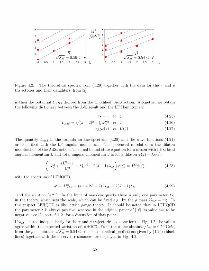
Figure 4.2: The theoretical spectra from (4.29) together with the data for the π and ρtrajectories and their daughters, from [2].
is then the potential UADS derived from the (modified) AdS action. Altogether we obtainthe following dictionary between the AdS result and the LF Hamiltonian:
x5 = z ⇔ ζ (4.25)
LAdS =√
(J − 2)2 + (µR)2 ⇔ L (4.26)
UADS(z) ⇔ U(ζ) (4.27)
The quantity LAdS in the formula for the spectrum (4.20) and the wave functions (4.21)are identified with the LF angular momentum. The potential is related to the dilatonmodification of the AdS5 action. The final bound state equation for a meson with LF orbitalangular momentum L and total angular momentum J is for a dilaton ϕ(z) = λMz
2:(−∂2
ζ +4L2 − 1
4ζ2+ λ2
Mζ2 + 2(J − 1)λM
)φ(ζ) = M2φ(ζ), (4.28)
with the spectrum of LFHQCD
q2 = M2nLJ = (4n+ 2L+ 2) |λM |+ 2(J − 1)λM (4.29)
and the solution (4.21). In the limit of massless quarks there is only one parameter λMin the theory, which sets the scale, which can be fixed e.g. by the ρ mass 2λM = m2
ρ. Inthis respect LFHQCD is like lattice gauge theory. It should be noted that in LFHQCDthe parameter λ is always positive, whereas in the original paper of [18] its value has to benegative, see [2], sect. 5.1.2. for a discussion of that point.
If λM is fitted independently for the π and ρ trajectories, as done for the Fig. 4.2, the valuesagree within the expected variation of ≈ ±10%. From the π one obtains
√λM = 0.59 GeV,
from the ρ one obtains√λM = 0.54 GeV. The theoretical predictions given by (4.29) (black
lines) together with the observed resonances are displayed in Fig. 4.2.
32
4.4 Bound state equations for baryons with arbitrary
spin
We present only the starting point and the final result and refer to [21] for a detailed presen-tation. Particles with half integer spin are generally described [22] by a spinor with additionaltensor indices, ΨN1···NT . In 4 and 5 dimensions such a relativistic spinor has 4 components.The starting point is the invariant Lagrangian for a spinor field. It turns out that a dilatonterm, that is a factor eλz
2in the the Lagrangian does not lead to an interaction [23], since
it can be absorbed by the fermion field, we therefore do not include it in the action. Inorder to get bound states one has to add a Yukawa like term ΨN1···NT λBz
2 ΨN ′1···N ′T to theLagrangian [23].
Our starting point is the action:
SFeff = 12
∫ddx dz
√g gN1N ′1 · · · gNT N ′T (4.30)[
ΨN1···NT
(iΓA eMA DM − µ− λB z2
)ΨN ′1···N ′T + h.c.
]Here ΨN1···NT is a spinor field in AdS5 with T = J − 1
2covariant indices, that is T = 0 for
the nucleon. The spinor is symmetric in the tensor indices. ΓA eMA are the Dirac matricesin AdS5 metric, eMA is the so called 4-bein of AdS, eMA = z
RδMA . The matrices ΓA are the
Dirac matrices of flat 5-dimensional space, ΓA = γA, Γ5 = iγ5. DMΨN1···NT is the covariantderivative of a spinor (it is even more complicated than the covariant derivative of a tensor,since it contains also the so called spin connection.). A symmetry breaking term has beeninserted: the Yukawa term ΨN1···NTλBz
2ΨN ′1···N ′T . As mentioned above, a term eϕ(z) like in(4.12) could also be inserted, but it has no influence on the equations of motion.
The procedure to obtain the equations of motion is the following1) We evaluate the Euler Lagrange equations:
∂K∂
∂(∂KΨN1···NT )L =
δLδΨN1···NT
; ∂K∂
∂(∂KΨN1···NT )L =
δLδΨN1···NT
(4.31)
and obtain equations, which can be brought into the form:[i
(zηMNΓM∂N +
4− 2T
2Γz
)− µR−Rλz2
]Ψν1...νT = 0. (4.32)
2) We set all spinor tensors, which have at least one index 5 to zero, that is all tensor-spinorfields have only Minkowski indicesΨν1···νT . Then we go to the momentum space
Ψν1···νT (q, z) =
∫d4xeiqxΨν1···νT (x, z) (4.33)
and extract the spin content by spinors which satisfy the Dirac equation:
(γq −M)uν1···νT (q) = 0, where M2 = q2. (4.34)
33
Then we define chiral spinors by u±ν1···νT (q) with
u±ν1···νT (q) = 12(1± γ5)uν1···νT (q) (4.35)
The original spinor field can be decomposed into the chiral components:
Ψν1···νT (q, z) = z2−T (u+ν1···νT (q)ψ+(q, z) + u−ν1···νT (q)ψ−(q, z)
)(4.36)
From (4.32) one obtains coupled first order differential equations for ψ±(q, z), by reciprocalinsertions they can be made to decouple and we finally obtaib(
−∂2z +
4L2AdS − 1
4z2+ λ2
Bz2 + 2(LAdS + 1)λB
)ψ+(q, z) = M2ψ+(q, z) (4.37)(
−∂2z +
4(LAdS + 1)2 − 1
4z2+ λ2
Bz2 + 2LAdS λB
)ψ−(q, z) = M2ψ−(q, z) (4.38)
withLAdS = |µR| − 1
2. (4.39)
We identify, as for the mesons, this quantity LAdS with the LF angular momentum L of thehadron, strictly speaking the LF angular momentum between a quark and the cluster.
These equations have the same structure as the one for bosons (4.14). The LF potential forthe two chirality components is:
U±(z) = λ2Bz
2 + 2(L+ 12± 1
2)λB (4.40)
that is it contains a quadratic confining term λ2Bz
2, as the meson potential (4.18), butdifferent constant terms.
By comparing with the results obtained in sect. 4.2 we obtain the spectrum:
M2nL = λB
(4n+ 2(L+ 1
2∓ 1
2) + 2 + 2(L+ 1
2± 1
2))
= 4λB(n+ L+ 1) (4.41)
and the same wave functions as the ones obtained for the mesons, see (4.21):
ψ+nL(q, z) = φnL(z), ψ−nL(q, z) = φnL+1(z) (4.42)
withφnL(z) = 1/N zL+1/2L(L)
n (|λ|z2)e−|λ|z2/2. (4.43)
Note that the two components of the baryon have different angular momentum. In the LFform the chirality + component has the spin aligned in +x3 direction, the − component in−x3 direction. If we speak of a baryon with spin L, we always refer to the L of the positivechirality component.
34
0 0.5 1 1.5 2 2.5 3
1
2
3
4
5
0 0.5 1 1.5 2 2.5 3
1
2
3
4
5
6
0 1 2 3 4 5 6
1
2
3
4
5
6
7
8
0 1 2 3 4 5 6
2
4
6
8
M2
[GeV2]
M2
[GeV2]
L L
L L
π√λM = 0.59 GeV
ρ√λM = 0.54 GeV
N√λB = 0.50 GeV
∆√λB = 0.52 GeV
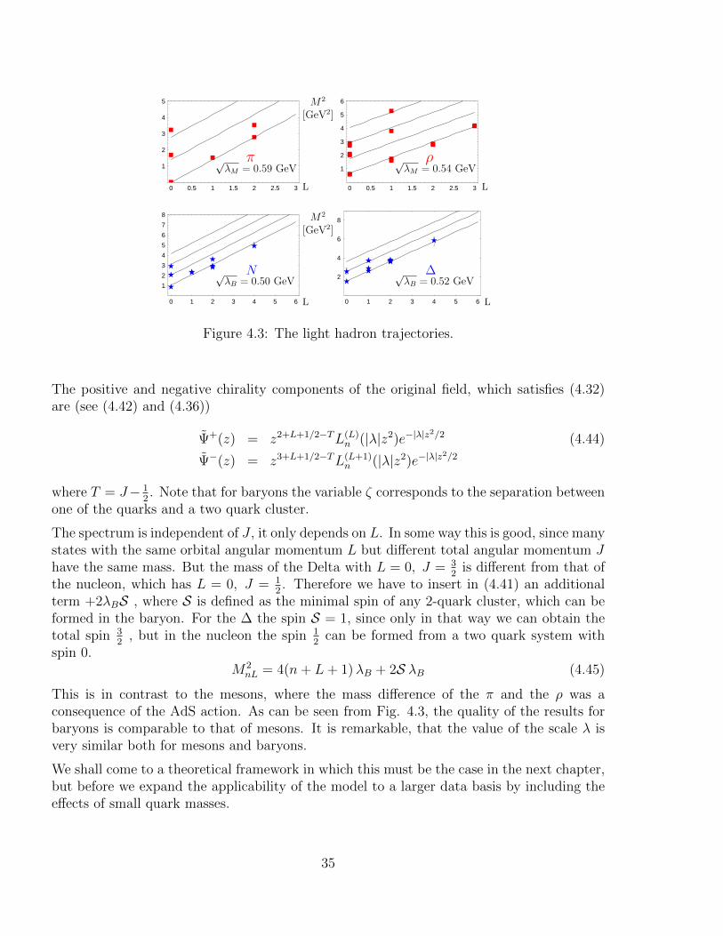
Figure 4.3: The light hadron trajectories.
The positive and negative chirality components of the original field, which satisfies (4.32)are (see (4.42) and (4.36))
Ψ+(z) = z2+L+1/2−TL(L)n (|λ|z2)e−|λ|z
2/2 (4.44)
Ψ−(z) = z3+L+1/2−TL(L+1)n (|λ|z2)e−|λ|z
2/2
where T = J− 12. Note that for baryons the variable ζ corresponds to the separation between
one of the quarks and a two quark cluster.
The spectrum is independent of J , it only depends on L. In some way this is good, since manystates with the same orbital angular momentum L but different total angular momentum Jhave the same mass. But the mass of the Delta with L = 0, J = 3
2is different from that of
the nucleon, which has L = 0, J = 12. Therefore we have to insert in (4.41) an additional
term +2λBS , where S is defined as the minimal spin of any 2-quark cluster, which can beformed in the baryon. For the ∆ the spin S = 1, since only in that way we can obtain thetotal spin 3
2, but in the nucleon the spin 1
2can be formed from a two quark system with
spin 0.M2
nL = 4(n+ L+ 1)λB + 2S λB (4.45)
This is in contrast to the mesons, where the mass difference of the π and the ρ was aconsequence of the AdS action. As can be seen from Fig. 4.3, the quality of the results forbaryons is comparable to that of mesons. It is remarkable, that the value of the scale λ isvery similar both for mesons and baryons.
We shall come to a theoretical framework in which this must be the case in the next chapter,but before we expand the applicability of the model to a larger data basis by including theeffects of small quark masses.
35
4.5 Inclusion of small quark masses
For small quark masses one expects that the mass effects can be treated in a perturbative way.Therefore one first tries perturbation theory. In the basic formula (4.1) for the constructionof the Hamiltonian,
M2 =
∫ 1
0
dx
∫d2k⊥ φ
LF∗(x,~k⊥)
(− 1
x(1− x)~k2⊥ +
m21
x+
m22
1− x
)φLF (x,~k⊥) + interaction
(4.46)the mass terms occur as
∑mixi
. Therefore a first guess for mass shift due to the quark massesis:
∆M2 =
∫ 1
0
(m2
1
x+
m22
1− x
)φLF (~b⊥, x)2 b⊥db⊥ dφ dx (4.47)
where φLF is the normalized LF wave function, see sect. 4.1. Inserting the relation (4.9) andusing x(1− x)b⊥db⊥ = ζ dζ one obtains
∆M2 =
∫dx
(m2
1
x+
m22
1− x
) ∫dζφ(ζ)2 (4.48)
where φ(ζ) is the normalized wave function (4.21). This expression for ∆M2 diverges!
Therefore we have to look for more realistic wave functions: The LF wave function (4.22)has the exponential behavior ∼ e−λx(1−x)b2⊥/2. Its Fourier transform is∫
d2b ei~b⊥~k⊥e−λx(1−x) b2⊥/2 =
2π
x(1− x)e−k
2⊥/(2λx(1−x)) (4.49)
The expressionk2⊥
x(1−x)in the wave function describes the off-energy shell behaviour in LF
form for massless quarks. Including quark masses, makes this quantity, see (4.1) :
k2⊥
x(1− x)+
(m2
1
x+
m22
1− x
)(4.50)
So it is plausible to include this factor also in the wave function, that is replace:
e−12λ
k2⊥x(1−x) → e
− 12λ
(k2⊥
x(1−x)+m2
1x
+m2
21−x
)(4.51)
This amounts to a multiplication of the wave functions with the factor
e−12λ
(m2
1x
+m2
21−x ) (4.52)
The modified normalized wave function is then:
φm =1
Ne−12λ
(m2
1x
+m2
21−x ) φ (4.53)
36
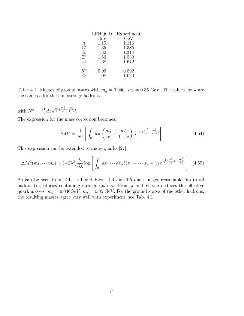
LFHQCD ExperimentGeV GeV
Λ 1.15 1.116Σ∗ 1.35 1.385Ξ 1.32 1.314Ξ∗ 1.50 1.530Ω 1.68 1.672
K∗ 0.90 0.892Φ 1.08 1.020
Table 4.1: Masses of ground states with mq = 0.046, ms = 0.35 GeV. The values for λ arethe same as for the non-strange hadrons.
with N2 =∫ 1
0dx e
−1λ
(m2
1x
+m2
21−x ).
The expression for the mass correction becomes:
∆M2 =1
N2
[∫ 1
0
dx
(m2
1
x+
m22
1− x
)e−1λ
(m2
1x
+m2
21−x )
](4.54)
This expression can be extended to many quarks [27]:
∆M2n(m1, · · ·mn) = (−2λ2)
∂
∂λlog
[∫ 1
0
dx1 · · · dxnδ(x1 + · · ·xn − 1) e−1λ
(m2
1x1
+···m2n
xn)
](4.55)
As can be seen from Tab. 4.1 and Figs. 4.4 and 4.5 one can get reasonable fits to allhadron trajectories containing strange quarks. From π and K one deduces the effectivequark masses: mq = 0.046GeV, ms = 0.35 GeV. For the ground states of the other hadrons,the resulting masses agree very well with experiment, see Tab. 4.1.
37
n 2 n 1 n 0M2IGeV2M
KH494L
HbL
L
K1H1270L
K1H1400LK2H1770L
K2H1820L
0 1 2 3
0
1
2
3
4
5
L
M2IGeV2M n 2 n 1 n 0
K*H892L
K*H1410L
K*H1680L
K2*H1430L
K3*H1780L
K4*H2045L
HbL
0 1 2 3 40
1
2
3
4
5
6
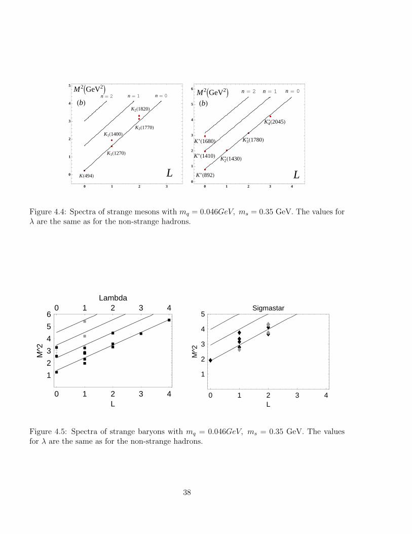
Figure 4.4: Spectra of strange mesons with mq = 0.046GeV, ms = 0.35 GeV. The values forλ are the same as for the non-strange hadrons.
0 1 2 3 4L
1
2
3
4
5
6
M^2
0 1 2 3 4Lambda
0 1 2 3 4L
1
2
3
4
5
M^2
Sigmastar
Figure 4.5: Spectra of strange baryons with mq = 0.046GeV, ms = 0.35 GeV. The valuesfor λ are the same as for the non-strange hadrons.
38
4.6 Summary
From the holographic principle one can derive wave functions for hadrons. By modifying theaction by suitable terms one can reproduce the spectrum of all hadrons containing only lightquarks within the expected accuracy. The form of the wave functions allows an interpretationof the quantities occurring in AdS5. The holographic variable can be identified with the LFvariable ζ, (4.3), and the product of the AdS mass µ and the curvature R is related to theLF angular momentum, see (4.15). By a well justified modification of the wave function dueto finite but small quark masses, one can describe all light hadrons in a satisfactory way, seeFigs. 4.3 – 4.5 .
There remain, however, two major unsatisfactory points: 1) The modification of the invariantAdS5 action was not determined by some theoretical principles but completely arbitrary andonly chosen to satisfy the data. 2) The observed similarity between meson and baryonspectra seems fortuitous, since the modification of the meson and baryon action has nothingin common, for mesons one multiplies the Lagrangian by a function, for baryons one has toadd a Yukawa-like term; the observed equality (within the expected accuracy) of the valuesof the fundamental parameters λM and λB seems also accidental. A third and minor pointis: that there was also no theoretical justification for adding the spin term 2Sλ to the baryonspectrum in (4.45).
In the next section we shall see that there is indeed a theoretical remedy for all theseunsatisfactory aspects.
39
Chapter 5
Supersymmetric light frontholographic QCD
The content of this chapter is based on the publications [24, 25, 27, 26].
The classical QCD Lagrangian contains in the limit of massless quarks no scale and is there-fore invariant under the conformal group in 4 dimensions 1 . In the AdS/CFT scheme, theaction of the quantum gauge theory shows an even larger symmetry, it is also invariant undersupersymmetry. Light Front Holographic QCD has approximated the quantum field theoryby a semiclassical theory (Quantum mechanics) by reducing the dynamics to a Light FrontHamiltonian with two constituents (or clusters of constituents) and a potential. This isfeasible, since in the limit of many colours in the gauge field theory all its features can be ob-tained by the classical solutions of an action in a 5 dimensional space. Quantum mechanics,and hence the semiclassical approximation, can be viewed as a quantum field theory in onedimension. It is therefore tempting to apply the symmetry constraints of the 4 dimensionalquantum field theory of the AdS/CFT correspondence also to the semiclassical theory, whichis a one-dimensional quantum field theory. In short we will discuss the consequences of animplementation of the superconformal (graded) algebra on our approach of light front holo-graphic QCD. Fortunately superconformal quantum mechanics is much simpler than generalsuperconformal field theory and notably it is a symmetry of wave functions and therefore itdoes not lead to the existence of new (stable ) particles which are the superpartners of theexisting particles. For pedagogical reasons we start with conformal symmetry, leaving thesuperconformal symmetry for the following section.
1Information on many concepts in this section, as conformal group, Noether theorem etc. can be foundconveniently in Wikipedia or Wikischolars.
40
5.1 Constraints from conformal algebra
Our aim is to incorporate into a semiclassical effective theory conformal symmetry. We willrequire that the corresponding one-dimensional effective action which encodes the confor-mal symmetry of QCD remains conformally invariant. De Alfaro, Fubini and Furlan [28]investigated in detail the simplest scale-invariant one-dimensional field theory, diven by theaction
A[Q] = 12
∫dt
(Q2 − g
Q2
)=
∫dtL, (5.1)
where Q ≡ dQ/dt. Since the action is dimensionless (in natural units), the dimension ofthe field Q must be half the dimension of the “time” variable t, dim[Q] = 1
2dim[t], and the
constant g is dimensionless. The translation operator in t, the Hamiltonian, is
H = 12
(Q2 +
g
Q2
), (5.2)
where the field momentum operator is P = ∂L∂Q
= Q, and the quantum equal time commu-
tation relation is[Q(t), Q(t)] = [Q(t), P (t)] = i. (5.3)
The equation of motion for the field operator Q(t) is given by the usual quantum mechanicalevolution
i [H,Q(t)] =dQ(t)
dt. (5.4)
Up to now we have worked in the Heisenberg picture: states are time independent, butoperators depend on time. Since we want to obtain a Schrodinger-like equation we go to theSchrodinger picture with time dependent states |ψ(t)〉 and time independent operators. Thetime dependence of the states is determined by the Hamiltonian:
H|ψ(t)〉 = id
dt|ψ(t)〉. (5.5)
We realize the states as elements of a Hilbert space of functions with one variable andtherefore the fields Q and P = Q are operators in that space. They are given by thesubstitution
Q(0)→ x, Q(0)→ −i ddx. (5.6)
Then we obtain the usual quantum mechanical evolution
i∂
∂tψ(x, t) = H
(x,−i d
dx
)ψ(x, t), (5.7)
Using (5.2) and (5.6) we obtain the familiar form
H = 12
(− d2
dx2+
g
x2
). (5.8)
41
It has the same structure as the LF Hamiltonian (4.24) with a vanishing light-front potential,as expected for a conformal theory. The dimensionless constant g in action (5.1) is nowrelated to the angular momentum in the light front wave equation (4.22).
As emphasized in [28], the absence of dimensional constants in (5.1) implies that the actionA[Q] is invariant under the full conformal group in one dimension, that is, under translations,dilatations, and special conformal transformations. These can be easily expressed by theinfinitesimal transformations of the variable t and the filed Q:
Translation t → t′ = t+ ε, Q→ Q′ = Q (5.9)
Dilatation t → t′ = t(1 + ε), Q→ Q′ = Q√
1 + ε (5.10)
spec. conf. transf. t → t′ =t
1− εt , Q→ Q′ =Q
1− εt (5.11)
One can convince oneself, that (5.1) is indeed invariant under these transformations. Inchecking this, be aware that ε is assumed to be infinitesimal, that is terms of O(ε2) must beneglected.
The constants of motion of the action are obtained by applying the Noether theorem. Theseconstants of motion are the generators of the conformal group. They are
Translations :
H(0) = 12
(Q2 +
g
Q2
), (5.12)
Dilatations:D(0) = −1
4
(QQ+QQ
)(5.13)
Special conformal transformations:
K(0) = 12Q2. (5.14)
Using the commutation relations (5.3) one can check that the operators H,D and K doindeed fulfill the algebra of the generators of the one-dimensional conformal group Conf (R1)
[H,D] = iH, [H,K] = 2 iD, [K,D] = −iK. (5.15)
The conventional Hamiltonian H is one of the generators of the conformal group. One canextend the concept of a Hamiltonian by forming a linear superposition of all three generators
G = uH + v D + wK. (5.16)
The new Hamiltonian G acts on the state vector and its evolution involves a new timevariable τ , which is related to t by
dτ =dt
u+ v t+ w t2. (5.17)
42
We now insert into (5.16) the expressions (5.12 – 5.14) and the Schrodinger picture substi-tutions (5.6) and obtain:
G =1
2u
(− d2
dx2+
g
x2
)+i
4v
(xd
dx+
d
dxx
)+
1
2wx2. (5.18)
Comparing with the LF Hamiltonian:
H = −∂2ζ +
4L2 − 1
4ζ2+ U(ζ); (5.19)
we see that the constraint to construct the Hamiltonian inside the conformal algebra restrictsthe possible forms of the potential considerably.
Comparing with the AdS-Hamiltonian for mesons(− ∂2
z +4L2 − 1
4ζ2+ λ2ζ2 + 2(J − 1)λ
)(5.20)
shows that with u = 2, w = λ2, v = 0, g = L2 − 14
the ”conformal Hamiltonian” G, (5.18),reproduces the ζ dependent terms of the AdS Hamiltonian for mesons.
This is very good, but not enough. We have also constant terms, which are essential for thespectra, and, above all we have baryons, therefore we also implement supersymmetry, whichrelates meson wave functions with baryon wave functions, that is we extend the conformalalgebra to the superconformal algebra.
5.2 Constraints from superconformal (graded) algebra
5.2.1 Supersymmetric QM
As mentioned in the Introduction, Supersymmetry (SUSY) relates particles of different spin.From a theorem of Coleman and Mandula follows, that this is impossible for symmetry groupsbased on algebras, like the rotational group, the gauge group SU(3) etc. It has been shownthat only symmetries based on generators which obey commutation and anti-commutationrules can do that. Such an extension of an algebra is called a graded algebra.
For a certain time, SUSY was very popular. Especially string theory is only fully consis-tent in a supersymmetric world. Supersymmetric QFT is very complicated. Moreoverthere is no sign in nature that it is realized, although the hopes were very high that onewould detect new particles which are supersymmetric partners of known ones. One hadeven speculated that supersymmetric partners of neutrinos might be good candidatesfor dark matter in cosmology. But since – at least up to now – no new particles, whichcould be supersymmetric partners, were found at LHCb, SUSY came in disrepute withphenomenologically interested physicists.
43
In contrast to SUSY Quantum Field theory, SUSY Quantum Mechanics is very simple [29]. It isbased on a graded algebra consisting of two “supercharges” (fermionic operators), Q and Q†, anda bosonic operator (the Hamiltonian) H. The two supercharges obey anticommutation relations,
Q,Q† = 2H, Q,Q = 0, Q†, Q† = 0
a supercharge and a bosonic operator obey commutation relations.
[Q,H] = 0, [Q†, H] = 0. 2
It is easy to realize this graded algebra as matrices in a Hilbert space with two components:
Q =
(0 −∂x + f
x + V (x)0 0
), Q† =
(0 0
∂x + fx + V (x) 0
)(5.21)
2H =
(−∂2
x + f2+fx2
+ V 2(x)− ∂xV (x) + 2f V (x)x 0
0 −∂2x + f2−f
x2+ V 2(x) + ∂xV (x) + 2f V (x)
x
)(5.22)
where f is a dimensionless constant and V has limx→0 xV (x) = 0, otherwise arbitrary.
5.2.2 Superconformal quantum mechanics
If the superpotential V vanishes, there is no dimensionful quantity in the game and we can extendthe SUSY algebra to a superconformal algebra [30, 31]. For V (x) = 0 the operators (5.21) become
Q = Q0 =
(0 −∂x + f
x0 0
), Q†0 =
(0 0
∂x + fx 0
)(5.23)
The absence of a dimensionful constant allows to extend the supersymmetric algebra to a super-conformal one. This is done by introducing a new supercharge S and its Hermitian adjoint S† withthe following anticommutation relations
S, S† = 2K, Q0, S† − Q†0S = 4iD, Q0, S
†+ Q†0, S = 2fI + σ3 (5.24)
all other anticommutators vanish
Q0, Q0 = Q0, S = S, S = Q†0, Q†0 = Q†0, S† = S†, S† = 0 (5.25)
Here K and D are the conformal operators introduced above. We see that the new superchargesS, S† extend the supersymmetric graded algebra to a superconformal one, which contains also thegenerators of the conformal algebra, introduced in the previous section. In matrix notation wehave:
S =(
0 x0 0
), S† =
(0 0x 0
), I =
(1 00 1
), σ3 =
(1 00 −1
). (5.26)
2Note that the operator 2H corresponds to the Meson Hamiltonian to be compared with the LF Hamil-tonian
44
5.2.3 Consequences of the superconformal algebra for dynamics
In subsection 5.1 a new Hamiltonian G was constructed inside the conformal algebra. Here weconstruct a new Hamiltonian inside the superconformal (graded) algebra. We now follow [24, 4] inapplying the procedure of [28], which was extended to the superconformal algebra by Fubini andRabinovici [31]and construct a generalized Hamiltonian. For that we introduce the supercharge Rλas linear combination of Q and S:
Rλ = Q0 + λS (5.27)
that is
Rλ =(
0 rλ0 0
), R† =
(0 0
r†λ 0
)(5.28)
with: rλ = −∂x + fx + λx, r†λ = ∂x + f
x + λx
The new generalized Hamiltonian is constructed analogously to the original one, but now not asan anticommutator of the supercharges Q and Q† , but as an anticommutator of the superchargesRλ and R†λ:
G = Rλ, R†λ = Q0, Q†0+ λ2S, S†+ λ
(Q0, S
†+ S,Q†0)
(5.29)
In this generalization of the Hamiltonian the dimensionful quantity λ appears naturally, since Sand Q have different physical dimension, Q has dimension [1/l] (1 over length), S has dimension[l], hence λ must have [l−2].
The new Hamiltonian G is diagonal:
G =
(rλ r
†λ 0
0 r†λ rλ
)=(G11 00 G22
)(5.30)
Supersymmetry implies that the two eigenvalues of G11 and G22 are identical. This can easilychecked:
Be φ =(φMφB
)an eigenvector of G, then we have
R†λGφ = ER†λ φ (5.31)
= R†λ(RλR†λ +R†λR)φ (5.32)
= R†RR†λφ since R†λR†λ = 0 (5.33)
= (RλR†λ +R†λR)R†λ φ (5.34)
= GR†λ φ (5.35)
That is if φ is eigenstate of G , then R†λφ is also eigenstate with the same eigenvalue. Let φ1 be
the state φ1 =(φM0
)and φ2 =
(0φB
), then
R†λφ1 =
(0
r†λφM
)(5.36)
has a lower component. Since it has the same eigenvalue as φ1, the two components have the sameeigenvalues.
45
We now construct the new Hamiltonian explicitly. Inserting (5.28) we obtain the explicit expressions
G11 = −∂2x +
4(f + 12)2 − 1
4x2+ λ2 x2 + 2λ (f − 1
2)︸ ︷︷ ︸U−
, (5.37)
G22 = −∂2x +
4(f − 12)2 − 1
4x2+ λ2 x2 + 2λ (f + 1
2)︸ ︷︷ ︸U+
. (5.38)
and compare this result with the Hamiltonians obtained from LFHQCD.
For the baryons we had obtained, see (4.37):(−∂2
z +4L2 − 1
4z2+ λ2
F z2 + 2(L+ 1)λF
)Ψ+(q, z) = M2Ψ+(q, z) (5.39)(
−∂2z +
4(L+ 1)2 − 1
4z2+ λ2
F z2 + 2LλF
)Ψ−(q, z) = M2Ψ−(q, z) (5.40)
and for mesons with J = L+ S, see (4.28)(− ∂2
z +4L2 − 1
4ζ2+ λ2ζ2 + 2(J − 1)λ
)ΦL,J(q, z) = q2ΦL,J(q, z) (5.41)
we identify f = L+ 12 and x = ζ and we notice two very nice features:
1)We recover the baryon equations (4.37)f. The potentials were in LFHQCD constructed with amodification of the AdS Lagrangian [24], which was there chosen ad hoc for purely phenomenologicalreasons. In superconformal LFHQCD the potentials are a consequence of the algebra. The chiralitytransformation, that is multiplication by γ5 acts like a supercharge.
2) G11 is the Hamiltonian of a meson with LM = J = f + 12 and G22 is the Hamiltonian of the
baryon component ψ+B with LB = f − 1
2 . So we can put the meson wave function φLM with LFangular momentum LM and the positive chirality baryon wave function ψ+
B with angular momentumLB = LM − 1 in a supersymmetric doublet:
Φ =
(φLMψ+LM−1
)(5.42)
The supercharge R†λ transforms the wave function of a boson into that of a fermion [4]. That is
Fermion and Boson wave functions are transformed into each other by a supercharge, namely R†λ,as it should be in supersymmetry !
The meson with angular momentum LM = f + 12 is superpartner of Baryon with LB = f − 1
2 ,therefore mesons with LM = 0 (π e.g.) can have no superpartner since LB = −1 is excluded. Onecan easily check that the lowest eigenstate φ0 of the Hamiltonian G has the eigenvalue 0 and theform
Φ0 =(φ000
), (5.43)
where φ00 is given by (4.21). This implies that there exists no nontrivial eigenstate of the baryonwith eigenvalue 0 which could be a partner of the lowest mesonic state. This is due to the fact thatr†λφ00 = 0.
46

Up to now we have only treated hadrons where the quark spin does not enter explicitly, like inthe pion and in the nucleon. in the next subsection the treatment will be extended to other cases,notably the rho-meson and the Delta resonance.
5.2.4 Spin terms and small quark masses
For mesons the action AdS distinguishes between the ρ trajectory, where the total quark spin S = 1,and the π trajectory, where the quark spin S = 0. Therefore the Hamiltonian (4.28) depends bothon the orbital angular L and on the total angular momentum. For mesons with J = L+ S, whereS is the total quark spin, we can separate the Hamiltonian (4.28) into a part containing only theangular momentum plus the spin term.
HM = HJ=L + 2S λ = G11 + 2S λ (5.44)
The Hamiltonian for a meson with J = L is identical with G11. Therefore we obtain as finalHamiltonian
GSUSY = Rλ, R†λ+ SI, (5.45)
where I is the unit operator; S is for mesons the total quark spin, and for baryons the minimalpossible quark spin of two-quark clusters inside baryon.
The supercharges Rλ, R†λ are given by (5.28) with f = LB+ 1
2 , they connect a baryon wave functionswith angular momentum LB and positive chirality and diquark spin S with a meson wave functionwith angular momentum LM = LB + 1 and total quark spin S.
In LFHQCD, sect. 4.4, the additional spin term in (4.45) had to be added for baryons by hand inorder to obtain agreement with experiment. In (5.45) it is a consequence of supersymmtry.
The corrections through finite quark masses will be the same as discussed in sect. 4.5 and will breakthe the supersymmetry. The final formulae for spectra from AdS with superconformal constraintsare:
Mesons M2M = 4λ(n+ LM ) + 2λS + ∆M2
2 (m1,m2), (5.46)
Baryons M2B = 4λ(n+ LB + 1) + 2λS + ∆M2
3 (m1,m2,m3).
Note that in applications of LFHQCD before 2016, e.g. in [2], for baryons with S = 1 the spineffect was taken into account by formally using half integer LF angular momentum; this leads tothe same mass formulæ.
5.2.5 Comparison with experiment
In Fig. 5.1 we display the theoretical curves obtained from (5.46) and the experimental results forthe non-strange hadrons, in Fig. 5.2 for hadrons containing 1 or 2 strange quarks. The result for theΩ− mass comes out to 1760 MeV, within the expected accuracy compatible with the experimentalmass of 1672 MeV. In Fig. 5.3 we display the values of
√λ obtained by independent fits to the
different chanels. Indicated at the abscissa are the lowest (L = 0) state of the trajectory. Theoryand experiment agree with the same accuracy of ≈ ±100 MeV, as expected from the model andalso observed in the previous chapter.
47
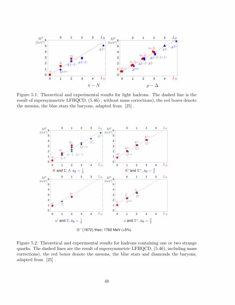
0 1 2 3 40
1
2
3
4
5
60 1 2 3M 2
[GeV2]
LM
LB
π
b1
π2
N1/2+
N12−, 3
2− N
32+, 5
2+
N92+
0 1 2 3 40
1
2
3
4
5
60 1 2 3M 2
[GeV2]
LM
LB
ρ, ω
a2, f2
a3, f3
a4, f4
Δ3/2+
Δ12−, 3
2−N
52−
Δ12+, 3
2+, 5
2+, 7
2+
N92−
Δ112
+
π −N ρ−∆
Figure 5.1: Theoretical and experimental results for light hadrons. The dashed line is theresult of supersymmetric LFHQCD, (5.46) , without mass corrections), the red boxes denotethe mesons, the blue stars the baryons, adapted from [25] .
0 1 2 3 40
1
2
3
4
5
60 1 2 3M 2
[GeV2]
LM
LB
K
K1
K2
Λ, ΣΛ
12−, 3
2−, Σ
12−, 3
2−
Λ32+, 5
2+
Λ72−
Λ92+
0 1 2 3 40
1
2
3
4
5
60 1 2 3M 2
[GeV2]
LM
LB
K∗
K2+
K3−
K4+
Σ3/2+
Σ52−
Σ72+
K and Σ,Λ, sB = 12 K∗and Σ∗, sB = 3
2
0 1 2 3 40
1
2
3
4
5
60 1 2 3M 2
[GeV2]
LM
LB
η′
η2
Ξ
0 1 2 3 40
1
2
3
4
5
60 1 2 3M 2
[GeV2]
LM
LB
φ
f ′2
φ3
Ξ3/2+
Ξ52−
η′ and Ξ, sB = 12 φ and Ξ∗, sB = 3
2
Ω−(1672) theo: 1760 MeV (+5%)
Figure 5.2: Theoretical and experimental results for hadrons containing one or two strangequarks. The dashed lines are the result of supersymmetric LFHQCD, (5.46), including masscorrections), the red boxes denote the mesons, the blue stars and diamonds the baryons,adapted from [25] .
48
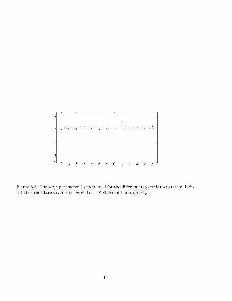
Figure 5.3: The scale parameter λ determined for the different trajectories separately. Indi-cated at the abscissa are the lowest (L = 0) states of the trajectory.
49
5.2.6 Completing the supersymmetric multiplet - Tetraquarks
Up to now we have only considered the supermultiplet of a meson and the positive chirality compo-nent of the baryon, Ψ+. The negative chirality component must also have a superpartner in orderto complete the supersymmetric multiplet. The supercharge R†λ transforms a meson wave functionwith LF angular momentum LB + 1 into a baryon wave function with angular momentum LB, itdecreases the angular momentum by one unit and changes the fermion number by 1, since it is afermionic operator.
R†(φLB+1
0
)=
(0
ψ+LB
)(5.47)
We can form a doublet containing the negative chirality component of the baryon Ψ−LB+1 (rememberthat the negative chirality component has an angular momentum one unit higher than the positiveone, see (4.42)): (
ψ−LB+1
φTLB
)(5.48)
where φTLB is a bosonic wave function with angular momentum LB, and it must be in the sameradial excitation state as the meson and the baryon. This is the only information we can drawfrom supersymmetric quantum mechanics, since it does not contain any information on the quarkstructure. One can only draw analog conclusions from the action of the operator R†λ inside the firstmultiplet, where the quark interpretation is fixed in LFHQCD.
In the original multiplet
(φLB+1
ψ+LB
)the operator R†λ has transformed a two-quark state into a
three-quark state, that it is has increased the number of constituents by 1. The two-quark statecould have colour 3 or 6, but it must be in a 3 colour state, since the baryon is a colour singlet.Therefore it is plausible to attribute to R†λ in the quark configuration the property of transformingan antiquark state into a two-quark state in the same colour representation 3, or correspondinglythe transformation of a quark into an two-antiquark state in the same colour 3 representation.From that we infer that R†λ transforms a quark of the nucleon into an antiquark pair in colour 3representation. Therefore we infer further that the superpartner of the negative chirality componentof the baryon is a tetraquark state consisting of a two quark state in colour 3 representation and atwo quark state in colour 3 representation. The previous considerations are graphically representedin Fig. 5.4.
The complete supersymmetric quadruplet can be arranged into a 2× 2 matrix,(φLB+1 ψ−LB+1
ψ+LB
φTLB
)(5.49)
with
G
(φLB+1 ψ−LB+1
ψ+LB
φTLB
)= M2
(φLB+1 ψ−LB+1
ψ+LB
φTLB
)(5.50)
It is important to note that the two-constituent clustering has only to be considered as a kinematical,but not as a dynamical grouping. We shall see later in treating the form factors that there isindeed no indication for a tightly bound diquark state. Therefore we must assume that there is noexcitation of the two constituent cluster. The Pauli principle implies then that the two-constituent
50

|ll|
R†λ
R†λ
R†λ
R†λ
-
-
-
-
|||lll
||llll||
Figure 5.4: Since particles and antiparticles are in this semiclassical theory treated at thesame footing, the fermionic operator R†λ can be interpreted either as transforming a quarkinto an antiquark pair (red arrows) or an antiquark into a quark pair (blue arrows). In thetransition from the meson to the nucleon the two-quark state has to be in the antisymmetriccolour representation. It is natural to require this also in the transition from the nucleon tothe tetraquark.
Table 5.1: Two candidates in the lowest possible angular momentum state.
Meson I(JP ) Baryon I(JP ) Tetraquark I(JP )
b1(1235) 1(1+) N+,−(940) 12(1
2
+) f0(980) 0(0+)
a2(1320) 1(2+) ∆+,−(1230) 32(3
2
+) a1(1260)1(1+)
cluster must be in an Isospin I = 1 and total angular J = 1 state or an I = 0, J = 0 state, since itis antisymmetric in colour and must also be totally antisymmetric. If the clusters are in a relativeS state, colour can rearrange and the 33 state can change into a 00 state since
3∑i=1
εijk εi`m = δ`j δ
mk − δ`k δmj (5.51)
This is a meson-molecule and can decay easily without further involvement of strong interactions.The status of tetraquarks is therefore rather uncertain, unless for some reason it is stable understrong interactions, when the decay threshold of the decay into to mesons is higher than he massof the tetraquark. Also higher orbital expiations make the colour rearrangement more difficult,because of the spatial separations of the two clusters by the centrifugal barrier. We considernevertheless in Table 5.1 two candidates for complete super-quadruplets in the lowest possibleangular momentum state: Though the agreement - always in the limits of the expected accuracy- is very satisfactory, one should take into account that there are also conventional interpretationsfor the states listed in the table under tetraquarks. We therefore do not pretend that these statesare pure tetraquark states, but that the tetraquark states should be taken into account if a detailedanalysis of states with similar masses and the same quantum numbers is performed.
51
5.3 Implications of supersymmetry on Hadrons con-
taining heavy quarks
This section is based on [25, 26].
We have seen in Fig. 5.2 that breaking of the conformal symmetry by small quark masses doesnot invalidate the principal results of superconformal LFHQCD, if the effect of the quark massesis taken into account perturbatively, see sects 4.5 and 5.2.4. In this section we investigate theinclusion of one heavy quark (c or b quark). The question is: Does the supersymmetric part of thesuperconformal algebra survive? The fact that supersymmetry played an essential role to fix theexact form of the potentials gives us some hope that it plays generally a fundamental role in theAdS/CFT correspondence and might even be present, if conformal symmetry is broken strongly byheavy quark masses.
5.3.1 The experimental situation
We have a look at the corresponding meson and baryon spectra where we plot both spectra in thesame graph and use the relation that the meson LF angular momentum is by one unit larger thanthat of its baryonic partner, LM = LB + 1. The results, displayed in Fig. 5.5 and Fig. 5.6 showthat supersymmetry is realized to a similar degree as for light quarks, and as far as one can see,there is even an indication for linear trajectories.
52
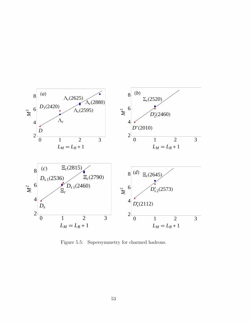
a
D
c
c2595
c2880D12420
c2625
0 1 2 32
4
6
8
LM LB 1
M2
D2010
D22460
c2520b
0 1 2 32
4
6
8
LM LB 1
M2
c
Ds
c
Ds 12536Ds 12460
c2790
c2815
0 1 2 32
4
6
8
LM LB 1
M2
Ds2112
Ds 2 2573
c2645d
0 1 2 32
4
6
8
LM LB 1
M2
Figure 5.5: Supersymmetry for charmed hadrons.
53
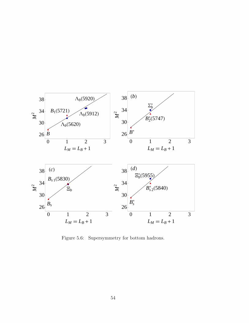
B
b5620
b5912
b5920
B15721
0 1 2 326
30
34
38
LM LB 1
M2
b
B
B25747
b
0 1 2 326
30
34
38
LM LB 1
M2
c
Bs
Bs 15830
b
0 1 2 326
30
34
38
LM LB 1
M2
d
Bs 2 5840
Bs
b5955
0 1 2 326
30
34
38
LM LB 1
M2
Figure 5.6: Supersymmetry for bottom hadrons.
54
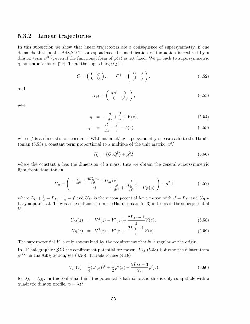
5.3.2 Linear trajectories
In this subsection we show that linear trajectories are a consequence of supersymmetry, if onedemands that in the AdS/CFT correspondence the modification of the action is realized by adilaton term eϕ(z), even if the functional form of ϕ(z) is not fixed. We go back to supersymmetricquantum mechanics [29]. There the supercharge Q is
Q =(
0 q0 0
), Q† =
(0 0q† 0
), (5.52)
and
HM =
(q q† 00 q†q
), (5.53)
with
q = − d
dz+f
z+ V (z), (5.54)
q† =d
dz+f
z+ V (z), (5.55)
where f is a dimensionless constant. Without breaking supersymmetry one can add to the Hamil-tonian (5.53) a constant term proportional to a multiple of the unit matrix, µ2I
Hµ = Q,Q†+ µ2I (5.56)
where the constant µ has the dimension of a mass; thus we obtain the general supersymmetriclight-front Hamiltonian
Hµ =
(− d2
dz2+
4L2M−1
4z2+ UM (z) 0
0 − d2
dz2+
4L2B−1
4z2+ UB(z)
)+ µ2 I (5.57)
where LB + 12 = LM − 1
2 = f and UM is the meson potential for a meson with J = LM and UB abaryon potential. They can be obtained from the Hamiltonian (5.53) in terms of the superpotentialV .
UM (z) = V 2(z)− V ′(z) +2LM − 1
zV (z), (5.58)
UB(z) = V 2(z) + V ′(z) +2LB + 1
zV (z). (5.59)
The superpotential V is only constrained by the requirement that it is regular at the origin.
In LF holographic QCD the confinement potential for mesons UM (5.58) is due to the dilaton termeϕ(x) in the AdS5 action, see (3.26). It leads to, see (4.18)
Udil(z) =1
4(ϕ′(z))2 +
1
2ϕ′′(z) +
2LM − 3
2zϕ′(z) (5.60)
for JM = LM . In the conformal limit the potential is harmonic and this is only compatible with aquadratic dilaton profile, ϕ = λz2.
55
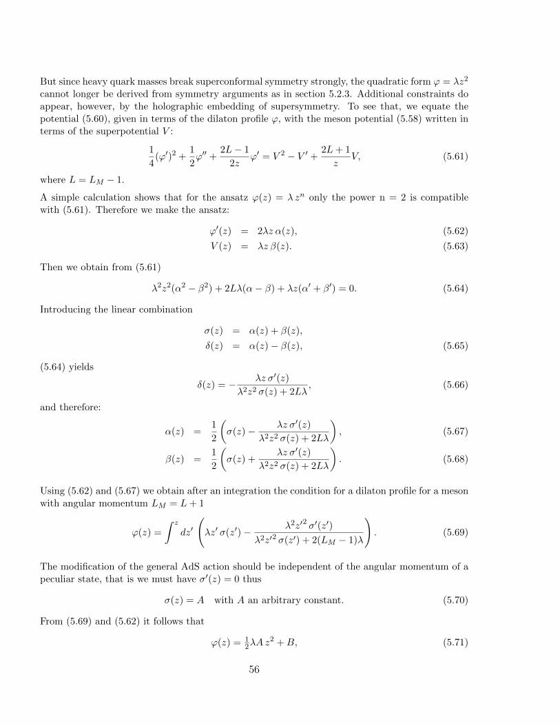
But since heavy quark masses break superconformal symmetry strongly, the quadratic form ϕ = λz2
cannot longer be derived from symmetry arguments as in section 5.2.3. Additional constraints doappear, however, by the holographic embedding of supersymmetry. To see that, we equate thepotential (5.60), given in terms of the dilaton profile ϕ, with the meson potential (5.58) written interms of the superpotential V :
1
4(ϕ′)2 +
1
2ϕ′′ +
2L− 1
2zϕ′ = V 2 − V ′ + 2L+ 1
zV, (5.61)
where L = LM − 1.
A simple calculation shows that for the ansatz ϕ(z) = λ zn only the power n = 2 is compatiblewith (5.61). Therefore we make the ansatz:
ϕ′(z) = 2λz α(z), (5.62)
V (z) = λz β(z). (5.63)
Then we obtain from (5.61)
λ2z2(α2 − β2) + 2Lλ(α− β) + λz(α′ + β′) = 0. (5.64)
Introducing the linear combination
σ(z) = α(z) + β(z),
δ(z) = α(z)− β(z), (5.65)
(5.64) yields
δ(z) = − λz σ′(z)λ2z2 σ(z) + 2Lλ
, (5.66)
and therefore:
α(z) =1
2
(σ(z)− λz σ′(z)
λ2z2 σ(z) + 2Lλ
), (5.67)
β(z) =1
2
(σ(z) +
λz σ′(z)λ2z2 σ(z) + 2Lλ
). (5.68)
Using (5.62) and (5.67) we obtain after an integration the condition for a dilaton profile for a mesonwith angular momentum LM = L+ 1
ϕ(z) =
∫ z
dz′(λz′ σ(z′)− λ2z′2 σ′(z′)
λ2z′2 σ(z′) + 2(LM − 1)λ
). (5.69)
The modification of the general AdS action should be independent of the angular momentum of apeculiar state, that is we must have σ′(z) = 0 thus
σ(z) = A with A an arbitrary constant. (5.70)
From (5.69) and (5.62) it follows that
ϕ(z) = 12λAz
2 +B, (5.71)
56
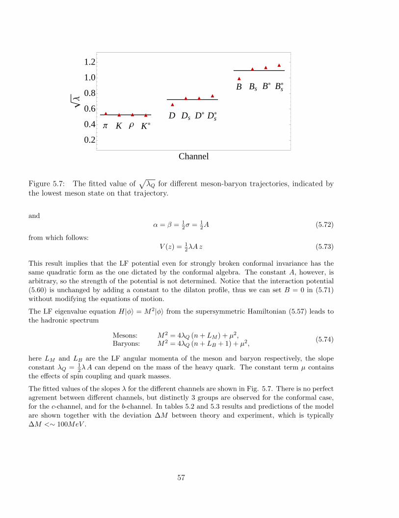
Π K Ρ KD Ds D Ds
B Bs B Bs
0.2
0.4
0.6
0.8
1.0
1.2
Channel
Λ
Figure 5.7: The fitted value of√λQ for different meson-baryon trajectories, indicated by
the lowest meson state on that trajectory.
andα = β = 1
2σ = 12A (5.72)
from which follows:V (z) = 1
2λAz (5.73)
This result implies that the LF potential even for strongly broken conformal invariance has thesame quadratic form as the one dictated by the conformal algebra. The constant A, however, isarbitrary, so the strength of the potential is not determined. Notice that the interaction potential(5.60) is unchanged by adding a constant to the dilaton profile, thus we can set B = 0 in (5.71)without modifying the equations of motion.
The LF eigenvalue equation H|φ〉 = M2|φ〉 from the supersymmetric Hamiltonian (5.57) leads tothe hadronic spectrum
Mesons: M2 = 4λQ (n+ LM ) + µ2,Baryons: M2 = 4λQ (n+ LB + 1) + µ2,
(5.74)
here LM and LB are the LF angular momenta of the meson and baryon respectively, the slopeconstant λQ = 1
2λA can depend on the mass of the heavy quark. The constant term µ containsthe effects of spin coupling and quark masses.
The fitted values of the slopes λ for the different channels are shown in Fig. 5.7. There is no perfectagrement between different channels, but distinctly 3 groups are observed for the conformal case,for the c-channel, and for the b-channel. In tables 5.2 and 5.3 results and predictions of the modelare shown together with the deviation ∆M between theory and experiment, which is typically∆M <∼ 100MeV .
57
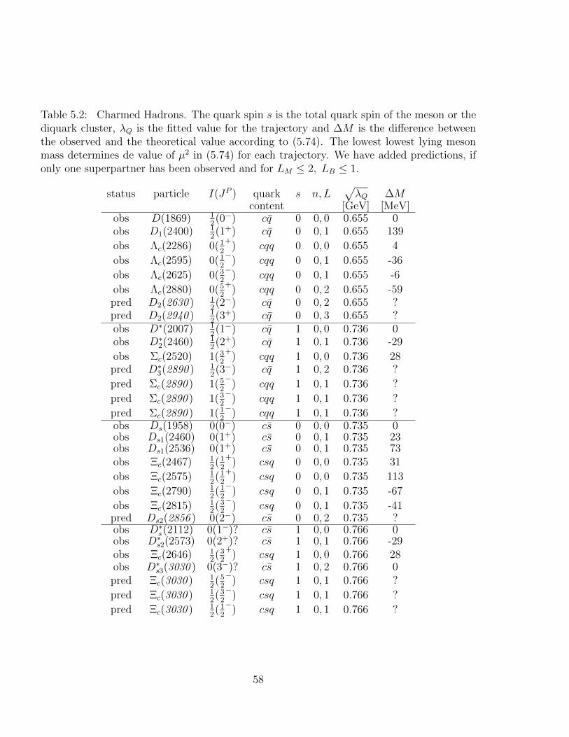
Table 5.2: Charmed Hadrons. The quark spin s is the total quark spin of the meson or thediquark cluster, λQ is the fitted value for the trajectory and ∆M is the difference betweenthe observed and the theoretical value according to (5.74). The lowest lowest lying mesonmass determines de value of µ2 in (5.74) for each trajectory. We have added predictions, ifonly one superpartner has been observed and for LM ≤ 2, LB ≤ 1.
status particle I(JP ) quark s n, L√λQ ∆M
content [GeV] [MeV]obs D(1869) 1
2(0−) cq 0 0, 0 0.655 0
obs D1(2400) 12(1+) cq 0 0, 1 0.655 139
obs Λc(2286) 0(12
+) cqq 0 0, 0 0.655 4
obs Λc(2595) 0(12
−) cqq 0 0, 1 0.655 -36
obs Λc(2625) 0(32
−) cqq 0 0, 1 0.655 -6
obs Λc(2880) 0(52
+) cqq 0 0, 2 0.655 -59
pred D2(2630 ) 12(2−) cq 0 0, 2 0.655 ?
pred D2(2940 ) 12(3+) cq 0 0, 3 0.655 ?
obs D∗(2007) 12(1−) cq 1 0, 0 0.736 0
obs D∗2(2460) 12(2+) cq 1 0, 1 0.736 -29
obs Σc(2520) 1(32
+) cqq 1 0, 0 0.736 28
pred D∗3(2890 ) 12(3−) cq 1 0, 2 0.736 ?
pred Σc(2890 ) 1(52
−) cqq 1 0, 1 0.736 ?
pred Σc(2890 ) 1(32
−) cqq 1 0, 1 0.736 ?
pred Σc(2890 ) 1(12
−) cqq 1 0, 1 0.736 ?
obs Ds(1958) 0(0−) cs 0 0, 0 0.735 0obs Ds1(2460) 0(1+) cs 0 0, 1 0.735 23obs Ds1(2536) 0(1+) cs 0 0, 1 0.735 73obs Ξc(2467) 1
2(1
2
+) csq 0 0, 0 0.735 31
obs Ξc(2575) 12(1
2
+) csq 0 0, 0 0.735 113
obs Ξc(2790) 12(1
2
−) csq 0 0, 1 0.735 -67
obs Ξc(2815) 12(3
2
−) csq 0 0, 1 0.735 -41
pred Ds2(2856 ) 0(2−) cs 0 0, 2 0.735 ?obs D∗s(2112) 0(1−)? cs 1 0, 0 0.766 0obs D∗s2(2573) 0(2+)? cs 1 0, 1 0.766 -29obs Ξc(2646) 1
2(3
2
+) csq 1 0, 0 0.766 28
obs D∗s3(3030 ) 0(3−)? cs 1 0, 2 0.766 0pred Ξc(3030 ) 1
2(5
2
−) csq 1 0, 1 0.766 ?
pred Ξc(3030 ) 12(3
2
−) csq 1 0, 1 0.766 ?
pred Ξc(3030 ) 12(1
2
−) csq 1 0, 1 0.766 ?
58
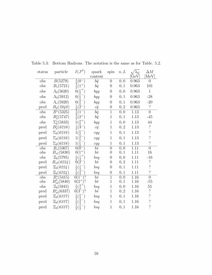
Table 5.3: Bottom Hadrons. The notation is the same as for Table. 5.2.
status particle I(JP ) quark spin n, L√λQ ∆M
content [GeV] [MeV]obs B(5279) 1
2(0−) bq 0 0, 0 0.963 0
obs B1(5721) 12(1+) bq 0 0, 1 0.963 101
obs Λb(5620) 0(12
+) bqq 0 0, 0 0.963 1
obs Λb(5912) 0(12
−) bqq 0 0, 1 0.963 -28
obs Λc(5920) 0(32
−) bqq 0 0, 1 0.963 -20
pred B2(5940 ) 12(2−) cq 0 0, 2 0.963 ?
obs B∗(5325) 12(1−) bq 1 0, 0 1.13 0
obs B∗2(5747) 12(2+) bq 1 0, 1 1.13 -45
obs Σ∗b(5833) 1(32
+) bqq 1 0, 0 1.13 44
pred B∗3(6216 ) 12(3−) cq 1 0, 2 1.13 ?
pred Σb(6216 ) 1(52
−) cqq 1 0, 1 1.13 ?
pred Σb(6216 ) 1(32
−) cqq 1 0, 1 1.13 ?
pred Σb(6216 ) 1(12
−) cqq 1 0, 1 1.13 ?
obs Bs(5367) 0(0−) bs 0 0, 0 1.11 0obs Bs1(5830) 0(1+) bs 0 0, 1 1.11 16obs Ξb(5795) 1
2(1
2
+) bsq 0 0, 0 1.11 -16
pred Bs2(6224 ) 0(2−) bs 0 0, 2 1.11 ?pred Ξb(6224 ) 1
2(1
2
−) bsq 0 0, 1 1.11 ?
pred Ξb(6224 ) 12(3
2
−) bsq 0 0, 1 1.11 ?
obs B∗s (5415) 0(1−)? bs 1 0, 0 1.16 0obs B∗s2(5840) 0(2+)? bs 1 0, 1 1.16 -55obs Ξb(5945) 1
2(3
2
+) bsq 1 0, 0 1.16 55
pred B∗s3(6337) 0(3−)? bs 1 0, 2 1.16 ?pred Ξb(6337 ) 1
2(5
2
−) bsq 1 0, 1 1.16 ?
pred Ξb(6337 ) 12(3
2
−) bsq 1 0, 1 1.16 ?
pred Ξb(6337 ) 12(1
2
−) bsq 1 0, 1 1.16 ?
59
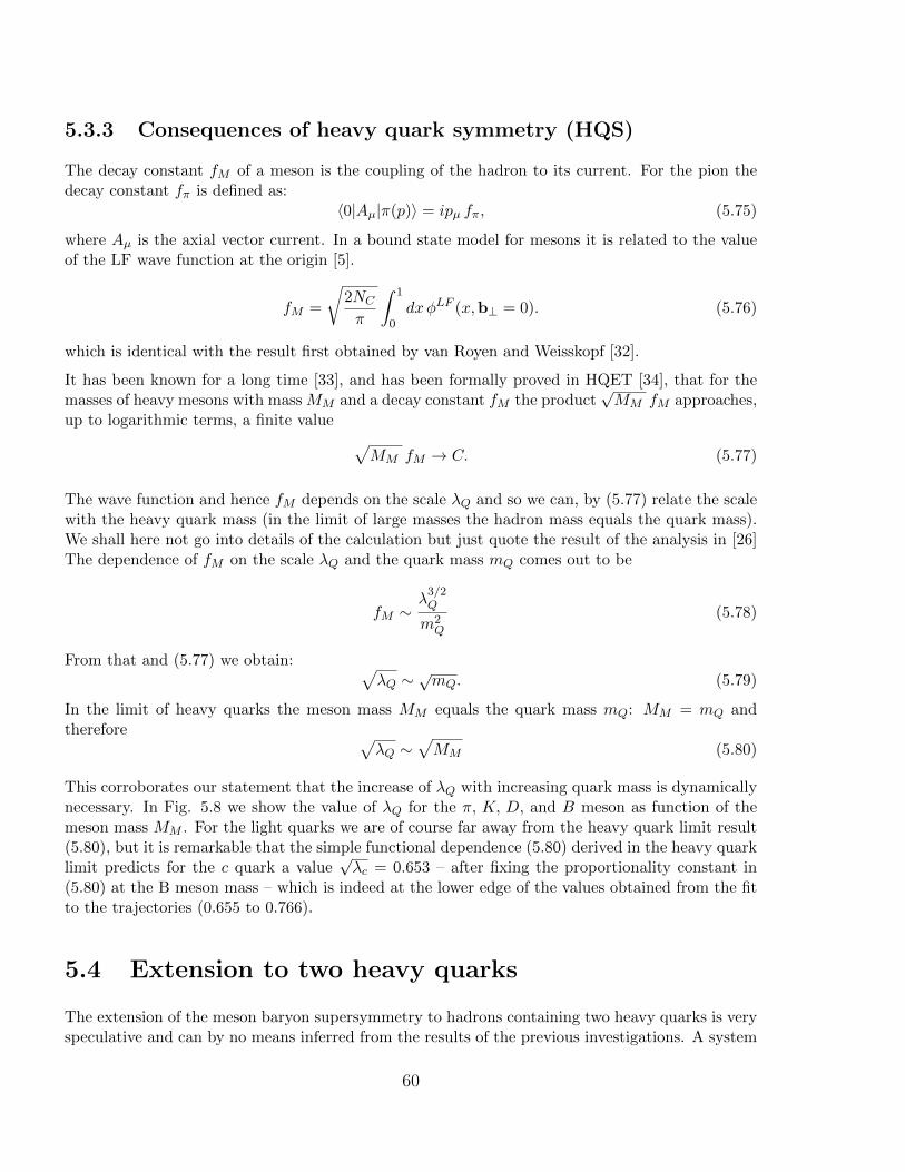
5.3.3 Consequences of heavy quark symmetry (HQS)
The decay constant fM of a meson is the coupling of the hadron to its current. For the pion thedecay constant fπ is defined as:
〈0|Aµ|π(p)〉 = ipµ fπ, (5.75)
where Aµ is the axial vector current. In a bound state model for mesons it is related to the valueof the LF wave function at the origin [5].
fM =
√2NC
π
∫ 1
0dxφLF (x,b⊥ = 0). (5.76)
which is identical with the result first obtained by van Royen and Weisskopf [32].
It has been known for a long time [33], and has been formally proved in HQET [34], that for themasses of heavy mesons with mass MM and a decay constant fM the product
√MM fM approaches,
up to logarithmic terms, a finite value √MM fM → C. (5.77)
The wave function and hence fM depends on the scale λQ and so we can, by (5.77) relate the scalewith the heavy quark mass (in the limit of large masses the hadron mass equals the quark mass).We shall here not go into details of the calculation but just quote the result of the analysis in [26]The dependence of fM on the scale λQ and the quark mass mQ comes out to be
fM ∼λ
3/2Q
m2Q
(5.78)
From that and (5.77) we obtain: √λQ ∼
√mQ. (5.79)
In the limit of heavy quarks the meson mass MM equals the quark mass mQ: MM = mQ andtherefore √
λQ ∼√MM (5.80)
This corroborates our statement that the increase of λQ with increasing quark mass is dynamicallynecessary. In Fig. 5.8 we show the value of λQ for the π, K, D, and B meson as function of themeson mass MM . For the light quarks we are of course far away from the heavy quark limit result(5.80), but it is remarkable that the simple functional dependence (5.80) derived in the heavy quarklimit predicts for the c quark a value
√λc = 0.653 – after fixing the proportionality constant in
(5.80) at the B meson mass – which is indeed at the lower edge of the values obtained from the fitto the trajectories (0.655 to 0.766).
5.4 Extension to two heavy quarks
The extension of the meson baryon supersymmetry to hadrons containing two heavy quarks is veryspeculative and can by no means inferred from the results of the previous investigations. A system
60
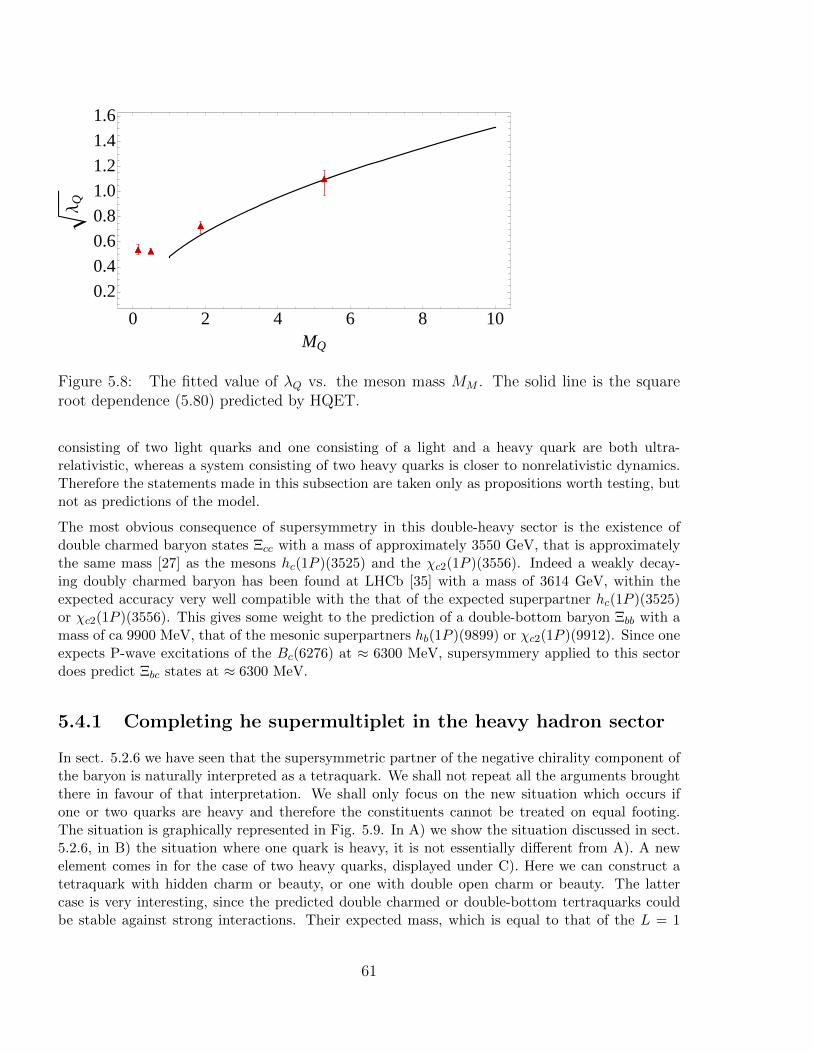
0 2 4 6 8 10
0.2
0.4
0.6
0.8
1.0
1.2
1.4
1.6
MQ
Λ Q
Figure 5.8: The fitted value of λQ vs. the meson mass MM . The solid line is the squareroot dependence (5.80) predicted by HQET.
consisting of two light quarks and one consisting of a light and a heavy quark are both ultra-relativistic, whereas a system consisting of two heavy quarks is closer to nonrelativistic dynamics.Therefore the statements made in this subsection are taken only as propositions worth testing, butnot as predictions of the model.
The most obvious consequence of supersymmetry in this double-heavy sector is the existence ofdouble charmed baryon states Ξcc with a mass of approximately 3550 GeV, that is approximatelythe same mass [27] as the mesons hc(1P )(3525) and the χc2(1P )(3556). Indeed a weakly decay-ing doubly charmed baryon has been found at LHCb [35] with a mass of 3614 GeV, within theexpected accuracy very well compatible with the that of the expected superpartner hc(1P )(3525)or χc2(1P )(3556). This gives some weight to the prediction of a double-bottom baryon Ξbb with amass of ca 9900 MeV, that of the mesonic superpartners hb(1P )(9899) or χc2(1P )(9912). Since oneexpects P-wave excitations of the Bc(6276) at ≈ 6300 MeV, supersymmery applied to this sectordoes predict Ξbc states at ≈ 6300 MeV.
5.4.1 Completing he supermultiplet in the heavy hadron sector
In sect. 5.2.6 we have seen that the supersymmetric partner of the negative chirality component ofthe baryon is naturally interpreted as a tetraquark. We shall not repeat all the arguments broughtthere in favour of that interpretation. We shall only focus on the new situation which occurs ifone or two quarks are heavy and therefore the constituents cannot be treated on equal footing.The situation is graphically represented in Fig. 5.9. In A) we show the situation discussed in sect.5.2.6, in B) the situation where one quark is heavy, it is not essentially different from A). A newelement comes in for the case of two heavy quarks, displayed under C). Here we can construct atetraquark with hidden charm or beauty, or one with double open charm or beauty. The lattercase is very interesting, since the predicted double charmed or double-bottom tertraquarks couldbe stable against strong interactions. Their expected mass, which is equal to that of the L = 1
61
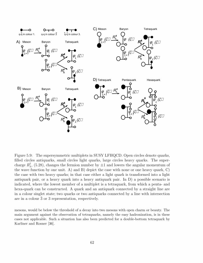
φ (ζ)
φ (ζ)
φ (ζ)φ (ζ)
L
L
L+1
L+1
φ (ζ)L
Rλ+
λRλ+
Rλ+Rλ+Rλ+Rλ+Rλ+λ+
φ (ζ)
φ (ζ)
φ (ζ)φ (ζ)
L
L
L+1
L+1
φ (ζ)L
Rλ+
λRλ+
Rλ+Rλ+Rλ+Rλ+Rλ+λ+
A)
B)
Meson Baryon Tetraquark
Meson Baryon Tetraquark
q-q in colour 1. q-q in colour 3 q-q in colour 3.-- - -
φ (ζ)
φ (ζ)
φ (ζ)φ (ζ)L
L
L+1
L+1
φ (ζ)L
Rλ+
λRλ+
Rλ+Rλ+Rλ+Rλ+Rλ+λ+
φ (ζ)L+1
Rλ+
φ (ζ)
φ (ζ)L+1
φ (ζ)L
φ (ζ)LλRλ+
Rλ+Rλ
+Rλ
+Rλ
+Rλ
+λ+
Meson Baryon Tetraquark
Tetraquark Pentaquark Hexaquark
C)
D)
Figure 5.9: The supersymmetric multiplets in SUSY LFHQCD. Open circles denote quarks,filled circles antiquarks, small circles light quarks, large circles heavy quarks. The super-charge R†λ, (5.28), changes the fermion number by ±1 and lowers the angular momentum ofthe wave function by one unit. A) and B) depict the case with none or one heavy quark, C)the case with two heavy quarks; in that case either a light quark is transformed into a lightantiquark pair, or a heavy quark into a heavy antiquark pair. In D) a possible scenario isindicated, where the lowest member of a multiplet is a tetraquark, from which a penta- andhexa-quark can be constructed. A quark and an antiquark connected by a straight line arein a colour singlet state; two quarks or two antiquarks connected by a line with intersectionare in a colour 3 or 3 representation, respectively.
mesons, would be below the threshold of a decay into two mesons with open charm or beauty. Themain argument against the observation of tetraquarks, namely the easy hadronization, is in thesecases not applicable. Such a situation has also been predicted for a double-bottom tetraquark byKarliner and Rosner [36].
62
5.5 Summary
If one imposes superconformal symmetry, more precisely expressed: if one demands that the gener-alized LF Hamiltonian is constructed from the generators of the (graded) superconformal algebra,all the problems mentioned in the summary of the last chapter are resolved. The LF potentialsfor mesons and baryons are unequivocally determined and we predict supermultiplets consistingof a meson with angular momentum LM , a baryon with angular momentum LB = LM − 1, anda bosonic state, which is plausibly interpreted as tetraquark, with angular momentum LB; thescale parameter λ is the same for mesons and baryons. The relations in the meson-baryon sector,encoded in the mass formulae (5.46) are satisfied by the data within the expected accuracy of ≈ 100MeV, see Figs. 5.1 and 5.2. Supersymmetry is also satisfied for hadrons containing one heavy quarkand perhaps even for hadrons with two heavy quarks, see sect. 5.3. Combining the conditions ofsupersymmetry with those of AdS one concludes that also hadrons containing a heavy quark lie onlinear trajectories, see sect. 5.3.2, Fig. 5.5 and 5.6. Heavy quark symmetry allows to estimate therelation between the λ-value for a system containing a c-quark and that for a system containinga b-quark, see Fig. 5.8. We again emphasize that the supersymmetry relates wave functions ofobserved mesons and observed baryons. There is no need nor motivation to introduce new particleslike squarks or gluinos.
63
Chapter 6
The propagator from AdS
6.1 The two point function in Holographic QCD
6.1.1 The generating functional
As shortly mentioned in the introduction, the generating functional (partition function in statisticalmechanics) allows to calculate all possible matrix elements and therefore all possible observables.
The generating functional for a quantum field φ is defined as
Z[j] =
∫Dφ ei
∫dxj(x)φ(x) eiS[φ] (6.1)
Here S[φ] is the AdS action and Dφ denotes the functional integration over all fields φ.
Unfortunately the functional integration can be performed analytically only for a Gaussian in-tegrand. This is the basis for perturbation theory, but for more general cases ones has to usenumerical methods (lattice calculations).
From the generating functional one can obtain all n-point functions by functional derivation. Thelatter – in contrast to functional integration – is elementary and can in general be performedanalytically. Functional derivatives occur also in classical field theory, for instance for the derivationof the classical equations of motion, see Chapt. 3.1. Indeed one can often ignore that a derivativeis a functional derivative. One considers the function, after which is derived, as a variable and usethe rules of ordinary differentiation.
The expression for the n-point function is:
〈T φ(x)φ(y)φ(z) . . . 〉 = (−i)n[(
δ
δj(x)
δ
δj(y)
δ
δj(z). . .
)Z[j]
]/j=0
(6.2)
Normally we are interested only in the connected n-point functions, corresponding to connectedFeynman diagrams. These are obtained from functional differentiation of the connected generating
64
functional W [j] which is the logarithm of Z[j]:
W [j] = logZ[j]. (6.3)
Ads/CFT allows to calculate the generating functional of the full quantum field theory (in theNc → ∞ limit) by solving the classical equations of motion of the 5-dimensional gravitationaltheory [9, 10]. One has to insert the classical solution, φ(x, z = ε) into the action and perform thelimit ε→ 0.
W [j] = i limε→0
S[φcl ]/ limε→0 φcl (ε)=j (6.4)
This essentially states that in the functional integral (6.1) only the fields which minimize the action,that is the classical solutions, contribute. We cannot insert directly the classical solution at z = 0into (6.4) since it contains infinities, as it is to be expected in a quantum field theory. We have toinsert the classical solution evaluated a finite value z = ε and the limit ε → 0 corresponds to therenormalization procedure. Generally it can be performed analytically as we shall see later.
6.1.2 The classical action
The classical action for mesons with arbitrary spin is (see sect. 4.2, (4.12))
Seff =
∫ddx dz
√g eϕ(z) gN1N ′1 · · · gNJN ′J
(gMM ′DMΦ∗N1...NJ
DM ′ΦN ′1...N′J
−µ2eff (z) Φ∗N1...NJ
ΦN ′1...N′J
). (6.5)
The covariant derivativesDM of higher rank tensors are very complicated (see sect. 3.1.2,footnote 1)but, as has been shown in [21], it turns out, that in the end one can largely ignore the complicationsand work as if the covariant derivatives were usual partial derivatives.
We proceed in the usual way,
1) we Fourier transform the solution of the Euler-Lagrange equations over the 4 Minkowski variables:ΦN1...NJ (q, z) =
∫d4xe−iqxΦN ′1...N
′J(x, z)
2) we extract the spin content into a spin tensor:Φ(q, z) = εN1···NJ Φ(q, z) where the spin tensor is totally symmetric in all indices and fulfills theconditions:
qN1 εN1···NJ (q) = 0, ηN1N2εN1N2···NJ (q) = 0 (6.6)
For the classical solutions in the 4 dimensional space (i.e. z = 0) we have ε5,N2,···NJ = 0, that isthe polarization tensor vanishes if at least one of the indices Ni = 5 . The factors in the integrand
of (6.5) are√g =
(Rz
)5, gN1N ′1 =
(zR
)2ηN1N ′1 and we obtain from (6.5):
S =
∫d4q
(2π)4S(q) (6.7)
with
S(q) = Xspin
∫ ∞ε
dz
(R
z
)3−2J
eϕ(z)[− ∂zΦ∗∂zΦ−
(−q2 +
(µR)2
z2
)Φ∗Φ
](6.8)
65
With the spin termXspin = σν1···νJ ,ν
′1···ν′J εν1···νJ εν′1···ν′J (6.9)
The term σν1···νJ ,ν′1···ν′J is due to the conditions (6.6). For J = 1 it is
σνν′
= ηνν′ − qν qν
′
q2(6.10)
We abbreviate:
A(z) =
(R
z
)3−2J
eϕ(z); B(z) =
(−q2 +
(µR)2
z2
)(6.11)
then the the action reads:
S(q) = Xspin
∫ ∞ε
dz(−A(z)∂zΦ
∗∂zΦ−B(z)A(z)Φ∗Φ)
(6.12)
The Euler Lagrange equations, of which the classical field Φcl is a solution, are
∂z∂L
∂(∂zΦ∗) =
∂L∂Φ∗
(6.13)
For solutions of the Euler Lagrange equations, that is the classical solutions Φcl (q, z) we havetherefore
− ∂z(A∂zΦcl
)= −AB Φcl (6.14)
We perform a partial integration for the first term of (6.12):
−∫ ∞ε
dz A(z)∂zΦ∗∂zΦ =
∫ ∞ε
dz Φ∗∂z(A∂zΦ)−[Φ∗A ∂zΦ
]∞ε
(6.15)
Inserting (6.14) into (6.12) we obtain:
S(q) =
∫ ∞ε
dz Φ∗cl (AB −AB)Φcl −[Φ∗cl A ∂zΦcl
]∞ε
(6.16)
The classical action is therefore reduced to a surface term.
Collecting everything we we obtain for the full action with the classical solution inserted:
S[Φcl ] = −Xspin
∫d4q
(2π)4
[(Rz
)3−2J
eϕ(z)Φ∗cl (q, z)∂zΦcl (q, z)]∞ε
(6.17)
We consider, as usual in field theory, only solutions which vanish at z →∞ and therefore only thelower surface term contributes and we end up with
S[Φcl ] = Xspin
∫d4q
(2π)4
[(Rz
)3−2J
eϕ(z)Φ∗cl (q, z)∂zΦcl (q, z)/z=ε (6.18)
In order to fulfill the condition limε→0 φcl (q, ε) = j(q) in (6.4) we choose the normalization
Φcl ,ν1 ···νJ (q, z) =Φcl (q, z)
Φcl (q, ε)jν1···νJ (q) (6.19)
66
So our final result is:
W [j] = i limε→0
S[φcl ]/ limε→0 φcl (ε)=j (6.20)
= i limz→ε→0
[σν1···νJ ,ν
′1···ν′J ×
∫d4q
(2π)4
(R
z
)3−2J
eϕ(z)j∗(q)ν1···νJΦ∗cl (q, z)
Φ∗cl (q, ε)j(q)ν′1···ν′J
∂zΦ(q, z)
Φ(q, ε)
]
= i σν1···νJ ,ν′1···ν′J
∫d4q
(2π)4eϕ(z)j∗(q)ν1···νJ j(q)ν′1···ν′J lim
z→ε→0
(R
z
)3−2J ∂zΦ(q, z)
Φ(q, ε)
The connected two point function is given by
Σν1···νJ ,ν′1···ν′J (q) = (−i)2 δ
δj∗ν1···νJ (q)
δ
δjν1···νJ (q)W [j]
=−i
(2π)4σν1ν
′1···νJν′J
(R
z
)3−2J
eϕ(z)
(∂zΦ(q, z)
Φ(q, ε)
)=
−i(2π)4
σν1ν′1···νJν′JΣ(q2) (6.21)
with
Σ(q2) =
(R
ε
)3−2J
eϕ(ε)
(∂zΦ(q, ε)
Φ(q, ε)
)(6.22)
It is always understood that ε→ 0.
As to be expected in QFT there will be infinities occurring in the limit ε → 0. These have tobe treated by some renormalization (this is not special to perturbation theory, but also has to bedone in lattice regularization, e.g.). If the infinities are independent of q, they are not dynamicallyrelevant and can be discarded. This will be done in the following.
6.2 Soft wall model
6.2.1 Solutions for soft wall model
Here we take ϕ(z) = λz2, that is the starting point is the same as in sect. 4.2. The Euler Lagrangeequation for the Lagrangian (6.5) is:[
∂2z +
1
z(2J − 3 + 2λz2)∂z + q2 − (µR)2
z2
]Φ(q, z) = 0 (6.23)
where in LFHQCD the AdS mass µ is related to the LF angular momentum L by (see (4.15))
L2 = (µR)2 + (J − 2)2. (6.24)
67
In sect. 4.2 we were interested in bound state solutions, which must be normalizable. This isonly possible for discrete values of q2 which led us to the hadronic spectra. If we give up thenormalizability condition, we shall find a larger set of solutions for every value of q2.
Mathematica finds a rather complicated solution for (6.23). So it is better to rescale Φ and bring(6.5) into a form which has relatively simple and mathematically well investigated solutions.
A rather general and well investigated form for a differential equation with first and second orderderivatives is Kummer’s equation [38], 13.1.1:
y w′′(y) + (b− y)w′(y)− aw = 0 (6.25)
with well studied solutions. This form can be obtained from (6.23) by rescaling.
We rescaleΦ(q, z) = zβΦn(q, z) (6.26)
and obtain [∂2z +
1
z(2J − 3 + 2β + 2λz2)∂z + q2 + C
]Φn(q, z) = 0 (6.27)
where
C =β2 + 2β(J − 2)− (µR)2
z2+ 2βλ+ q2 (6.28)
We can make the term ∼ 1/z2 vanish by choosing:
β = 2 + L− J, L =√
(J − 2)2 + (µR)2 (6.29)
We introduce the dimensionless variable
y = |λ|z2 (6.30)
and use: ∂zf(y) = ∂yf(y)2|λ|z, ∂2zf(y) = ∂2
yf(y)4λ2z2 + ∂yf(y)2|λ|Then we obtain with choice β = 2 + L− J from (6.27) the differential equation:
y ∂2y Φn(q, y) +
((L+ 1) +
λ
|λ| y)∂yΦn(q, y) + (6.31)
1
4|λ|(
(4− 2J + 2L)λ+ q2))
Φn(q, y) = 0
which has indeed the form of Kummer’s equation (6.25)
The solutions of (6.25) which vanish for z →∞ are:
w(y) = U(a, b, y). (6.32)
U(a, b, y) is the hypergeometric function (HypergeometriU[a,b,y] in Mathematica).
For the case of a positive sign in front the the term y w′(y) that is for the equation
y w′′(y) + (b+ y)w′(y)− aw = 0 (6.33)
68
the solution isw(y) = e−y U(a+ b, b, y) (6.34)
The solution Φ(q, y) of (6.23) has thus the form:
Φ(q, z) = ρ(z)U(aλ, L+ 1, |λ|z2
)(6.35)
with ρ(z) = zL−J+2e−(|λ|+λ)z2/2.
The constant aλ depends on the sign of λ:
for λ < 0 we have (6.32) and from (6.31)
λ < 0 aλ = − q2
4|λ| −λ
4|λ|(4− 2J + 2L)
= − q2
4|λ| +1
4(4− 2J + 2L) (6.36)
for λ > 0 we have (6.34) and from (6.31)
λ > 0 aλ = − q2
4|λ| −λ
4|λ|(4− 2J + 2L) + (L+ 1)
= − q2
4|λ| +1
4(2J + 2L) (6.37)
6.2.2 The propagator for the conserved current in the holographicsoft wall model
We use the general result (6.22) and insert (6.35) (omitting terms, which are 1 in the limit ε→ 0.
Σ[q2] =
(R
z
)3−2J
∂z[log[ρ[z]U(aλ, L+ 1, λz2)]/z→ε (6.38)
=
(R
z
)3−2J
∂z[log[U(aλ, L+ 1, λz2)]/z→ε + ∂z[log[ρ[z]]/z=ε→0
(6.39)
=
(R
z
)3−2J U ′(aλ, L+ 1, |λ|z2) 2|λ|zU(aλ, L+ 1, |λ|z2)
/z=ε→0
+ non-dynamical terms (6.40)
where non-dynamical terms are (possibly infinite) terms which are independent of q.
We see that multiplying the solution (6.35) with a function f(z) which is regular at z = 0 has noinfluence on the two point function.
In order to perform the limit ε → 0 we have to expand the ratio U ′/U around z = 0. It is mosttransparent to use the identity ([38], 13.4.21)
U ′(a, b, y) = −aU(a+ 1, b+ 1, y) (6.41)
from which we get the final result[39, 2]:
Σ[q] =
(R
z
)3−2J −aλ U(aλ + 1, L+ 2, |λ|z2) 2|λ|zU(aλ, L+ 1, |λ|z2)
/z=ε→0
(6.42)
69
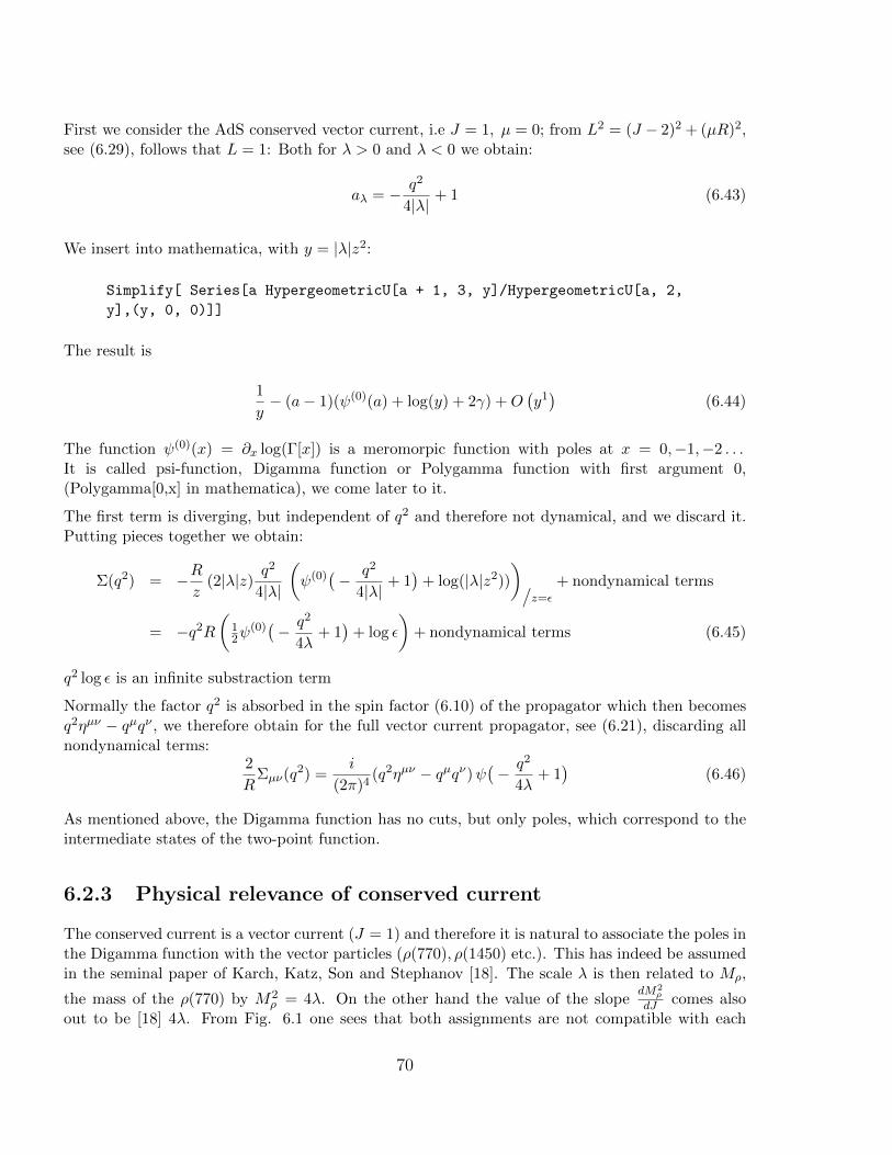
First we consider the AdS conserved vector current, i.e J = 1, µ = 0; from L2 = (J − 2)2 + (µR)2,see (6.29), follows that L = 1: Both for λ > 0 and λ < 0 we obtain:
aλ = − q2
4|λ| + 1 (6.43)
We insert into mathematica, with y = |λ|z2:
Simplify[ Series[a HypergeometricU[a + 1, 3, y]/HypergeometricU[a, 2,
y],(y, 0, 0)]]
The result is
1
y− (a− 1)(ψ(0)(a) + log(y) + 2γ) +O
(y1)
(6.44)
The function ψ(0)(x) = ∂x log(Γ[x]) is a meromorpic function with poles at x = 0,−1,−2 . . .It is called psi-function, Digamma function or Polygamma function with first argument 0,(Polygamma[0,x] in mathematica), we come later to it.
The first term is diverging, but independent of q2 and therefore not dynamical, and we discard it.Putting pieces together we obtain:
Σ(q2) = −Rz
(2|λ|z) q2
4|λ|
(ψ(0)
(− q2
4|λ| + 1)
+ log(|λ|z2))
)/z=ε
+ nondynamical terms
= −q2R
(12ψ
(0)(− q2
4λ+ 1)
+ log ε
)+ nondynamical terms (6.45)
q2 log ε is an infinite substraction term
Normally the factor q2 is absorbed in the spin factor (6.10) of the propagator which then becomesq2ηµν − qµqν , we therefore obtain for the full vector current propagator, see (6.21), discarding allnondynamical terms:
2
RΣµν(q2) =
i
(2π)4(q2ηµν − qµqν)ψ
(− q2
4λ+ 1)
(6.46)
As mentioned above, the Digamma function has no cuts, but only poles, which correspond to theintermediate states of the two-point function.
6.2.3 Physical relevance of conserved current
The conserved current is a vector current (J = 1) and therefore it is natural to associate the poles inthe Digamma function with the vector particles (ρ(770), ρ(1450) etc.). This has indeed be assumedin the seminal paper of Karch, Katz, Son and Stephanov [18]. The scale λ is then related to Mρ,
the mass of the ρ(770) by M2ρ = 4λ. On the other hand the value of the slope
dM2ρ
dJ comes alsoout to be [18] 4λ. From Fig. 6.1 one sees that both assignments are not compatible with each
70
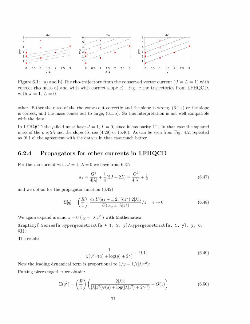
0 0.5 1 1.5 2 2.5 3J-1
1
2
3
4
5
6
M^2
rho
0 0.5 1 1.5 2 2.5 3J-1
1
2
3
4
5
6
M^2
rho
0 0.5 1 1.5 2 2.5 3L
1
2
3
4
5
6
M^2
rho
Figure 6.1: a) and b) The rho-trajectory from the conserved vector current (J = L = 1) withcorrect rho mass a) and with with correct slope c) , Fig. c the trajectories from LFHQCD,with J = 1, L = 0.
other. Either the mass of the rho comes out correctly and the slope is wrong, (6.1.a) or the slopeis correct, and the mass comes out to large, (6.1.b). So this interpretation is not well compatiblewith the data.
In LFHQCD the ρ-field must have J = 1, L = 0, since it has parity 1−. In that case the squaredmass of the ρ is 2λ and the slope 4λ, see (4.29) or (5.46). As can be seen from Fig. 4.2, repeatedas (6.1.c) the agreement with the data is in that case much better.
6.2.4 Propagators for other currents in LFHQCD
For the rho current with J = 1, L = 0 we have from 6.37:
aλ =Q2
4|λ| +1
4(2J + 2L) =
Q2
4|λ| + 12 (6.47)
and we obtain for the propagator function (6.42)
Σ[q] =
(R
z
)aλ U(aλ + 1, 2, |λ|z2) 2|λ|z
U(aλ, 1, |λ|z2)
/z = ε→ 0 (6.48)
We again expand around z = 0 ( y = |λ|z2 ) with Mathematica
Simplify[ Series[a HypergeometricU[a + 1, 2, y]/HypergeometricU[a, 1, y], y, 0,
0]];
The result:
− 1
y(ψ(0)(a) + log(y) + 2γ)+O[1] (6.49)
Now the leading dynamical term is proportional to 1/y = 1/(|λ|z2):
Putting pieces together we obtain:
Σ(q2) =
(R
z
)(2|λ|z
|λ|z2(ψ(a) + log(|λ|z2) + 2γE)+O(z)
)(6.50)
71
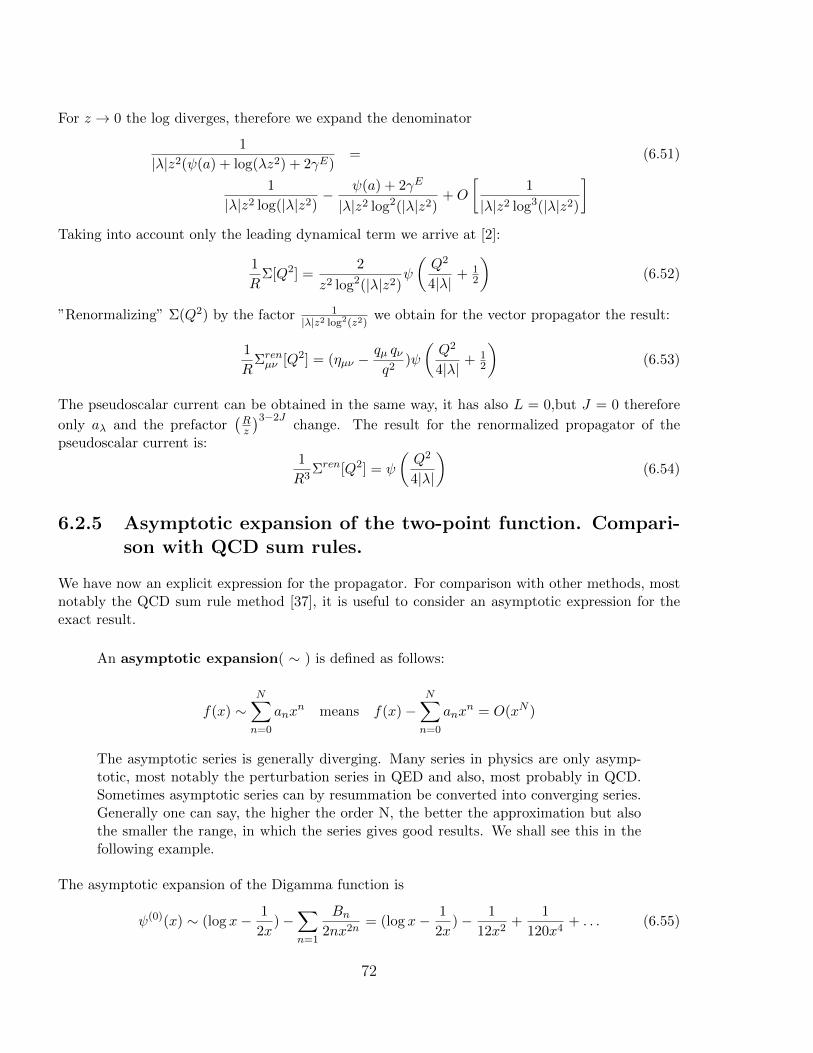
For z → 0 the log diverges, therefore we expand the denominator
1
|λ|z2(ψ(a) + log(λz2) + 2γE)= (6.51)
1
|λ|z2 log(|λ|z2)− ψ(a) + 2γE
|λ|z2 log2(|λ|z2)+O
[1
|λ|z2 log3(|λ|z2)
]Taking into account only the leading dynamical term we arrive at [2]:
1
RΣ[Q2] =
2
z2 log2(|λ|z2)ψ
(Q2
4|λ| + 12
)(6.52)
”Renormalizing” Σ(Q2) by the factor 1|λ|z2 log2(z2)
we obtain for the vector propagator the result:
1
RΣrenµν [Q2] = (ηµν −
qµ qνq2
)ψ
(Q2
4|λ| + 12
)(6.53)
The pseudoscalar current can be obtained in the same way, it has also L = 0,but J = 0 therefore
only aλ and the prefactor(Rz
)3−2Jchange. The result for the renormalized propagator of the
pseudoscalar current is:1
R3Σren[Q2] = ψ
(Q2
4|λ|
)(6.54)
6.2.5 Asymptotic expansion of the two-point function. Compari-son with QCD sum rules.
We have now an explicit expression for the propagator. For comparison with other methods, mostnotably the QCD sum rule method [37], it is useful to consider an asymptotic expression for theexact result.
An asymptotic expansion( ∼ ) is defined as follows:
f(x) ∼N∑n=0
anxn means f(x)−
N∑n=0
anxn = O(xN )
The asymptotic series is generally diverging. Many series in physics are only asymp-totic, most notably the perturbation series in QED and also, most probably in QCD.Sometimes asymptotic series can by resummation be converted into converging series.Generally one can say, the higher the order N, the better the approximation but alsothe smaller the range, in which the series gives good results. We shall see this in thefollowing example.
The asymptotic expansion of the Digamma function is
ψ(0)(x) ∼ (log x− 1
2x)−
∑n=1
Bn2nx2n
= (log x− 1
2x)− 1
12x2+
1
120x4+ . . . (6.55)
72
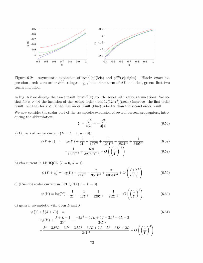
0.4 0.5 0.6 0.7 0.8 0.9 1x
-1
-0.9
-0.8
-0.7
-0.6
-0.5x
psi
0.4 0.5 0.6 0.7 0.8 0.9 1x
-2.5
-2
-1.5
-1
-0.5
psi
Figure 6.2: Asymptotic expansion of xψ(0)(x)(left) and ψ(0)(x)(right) . Black: exact ex-pression , red: zero order ψ(0) ≈ log x− 1
2x, blue: first term of AE included, green: first two
terms included.
In Fig. 6.2 we display the exact result for ψ(0)(x) and the series with various truncations. We seethat for x > 0.6 the inclusion of the second order term 1/(120x4)(green) improves the first orderresult, but that for x < 0.6 the first order result (blue) is better than the second order result.
We now consider the scalar part of the asymptotic expansion of several current propagators, intro-ducing the abbreviation:
Y =Q2
4|λ| = − q2
4|λ| (6.56)
a) Conserved vector current (L = J = 1, µ = 0):
ψ(Y + 1) = log(Y ) +1
2Y− 1
12Y 2+
1
120Y 4− 1
252Y 6+
1
240Y 8(6.57)
− 1
132Y 10+
691
32760Y 12+O
((1
Y
)13)
(6.58)
b) rho current in LFHQCD (L = 0, J = 1)
ψ(Y + 1
2
)= log(Y ) +
1
24Y 2− 7
960Y 4+
31
8064Y 6+O
((1
Y
)8)
(6.59)
c) (Pseudo) scalar current in LFHQCD (J = L = 0)
ψ (Y ) = log(Y )− 1
2Y− 1
12Y 2+
1
120Y 4− 1
252Y 6+O
((1
Y
)8)
(6.60)
d) general asymptotic with open L and J :
ψ(Y + 1
2(J + L))
= (6.61)
log(Y ) +J + L− 1
2Y+−3J2 − 6JL+ 6J − 3L2 + 6L− 2
24Y 2
+J3 + 3J2L− 3J2 + 3JL2 − 6JL+ 2J + L3 − 3L2 + 2L
24Y 3+O
((1
Y
)4)
73
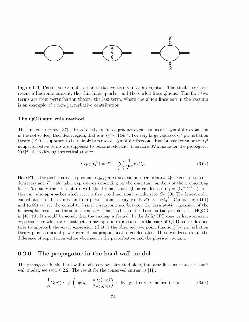
Figure 6.3: Perturbative and non-perturbative terms in a propagator. The thick lines rep-resent a hadronic current, the thin lines quarks, and the curled lines gluons. The first twoterms are from perturbation theory, the last term, where the gluon lines end in the vacuumis an example of a non-perturbative contribution
The QCD sum rule method
The sum rule method [37] is based on the operator product expansion as an asymptotic expansionin the not so deep Euclidean region, that is at Q2 ≈ 1GeV . For very large values of Q2 perturbationtheory (PT) is supposed to be reliable because of asymptotic freedom. But for smaller values of Q2
nonperturbative terms are supposed to become relevant. Therefore SVZ made for the propagatorΣ(Q2) the following theoretical ansatz:
ΣSV Z(Q2) = PT +∑n=1
1
Q2nFnC2n (6.62)
Here PT is the perturbative expression, C2n+2 are universal non-perturbative QCD constants (con-densates) and Fn calculable expressions depending on the quantum numbers of the propagatingfield. Normally the series starts with the 4-dimensional gluon condensate C4 = 〈GAµνGAµν〉, butthere are also approaches which start with a two dimensional condensate, C2 [39]. The lowest ordercontribution to the expression from perturbation theory yields PT ∼ logQ2. Comparing (6.61)and (6.62) we see the complete formal correspondence between the asymptotic expansion of theholographic result and the sum rule ansatz. This has been noticed and partially exploited in HQCDin [40, 39]. It should be noted, that the analogy is formal. In the AdS/CFT case we have an exactexpression for which we construct an asymptotic expression. In the case of QCD sum rules onetries to approach the exact expression (that is the observed two point function) by perturbationtheory plus a series of power corrections proportional to condensates. These condensates are thedifference of expectation values obtained in the perturbative and the physical vacuum.
6.2.6 The propagator in the hard wall model
The propagator in the hard wall model can be calculated along the same lines as that of the softwall model, see sect. 6.2.2. The result for the conserved current is [41]:
1
RΣ(q2) ∼ q2
(log(q)− π Y0(qz0)
2 J0(qz0)
)+ divergent non-dynamical terms (6.63)
74
It is a meromorphic function with poles at the zeros of the Bessel function J0. The logarithmic cutof the Bessel function Y0 cancels the explicitly occurring logarithm. In this case the propagatorhas no asymptotic expansion with a logarithm and additional power corrections as in the soft wallmodel (6.55) and there is no formal similarity with the expression used in QCD sum rules. Indeed,as has been shown in [41], the hard wall model is rather the equivalent of a model developed byMigdal [42]. In this model the perturbative expression (the logarithm) is approximated by a (finite)sum of pole terms.
6.3 Summary
The propagator of a mesons in the soft wall model is a digamma function, which is meromorphic.The asymptotic expansion of the digamma function for negative arguments shows a remarkablestructural similarity with the expansion of the propagator used for QCD sum rules.
75
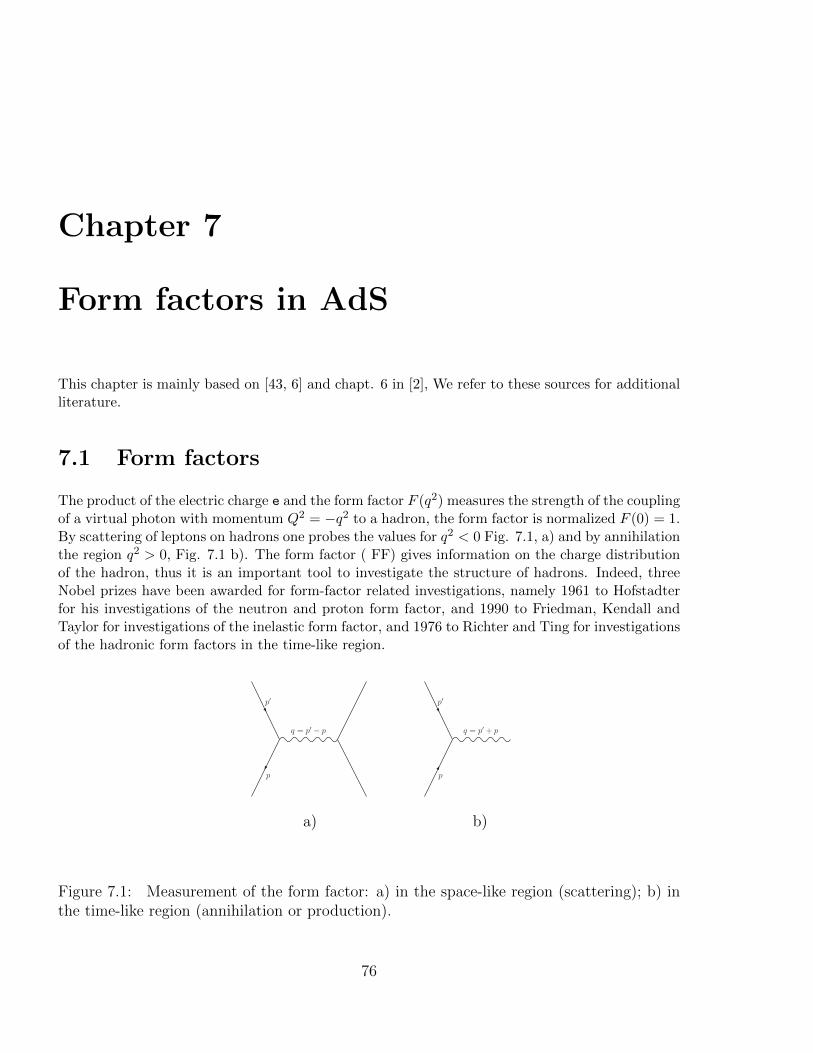
Chapter 7
Form factors in AdS
This chapter is mainly based on [43, 6] and chapt. 6 in [2], We refer to these sources for additionalliterature.
7.1 Form factors
The product of the electric charge e and the form factor F (q2) measures the strength of the couplingof a virtual photon with momentum Q2 = −q2 to a hadron, the form factor is normalized F (0) = 1.By scattering of leptons on hadrons one probes the values for q2 < 0 Fig. 7.1, a) and by annihilationthe region q2 > 0, Fig. 7.1 b). The form factor ( FF) gives information on the charge distributionof the hadron, thus it is an important tool to investigate the structure of hadrons. Indeed, threeNobel prizes have been awarded for form-factor related investigations, namely 1961 to Hofstadterfor his investigations of the neutron and proton form factor, and 1990 to Friedman, Kendall andTaylor for investigations of the inelastic form factor, and 1976 to Richter and Ting for investigationsof the hadronic form factors in the time-like region.
p′
p
q = p′ − p
p′
p
q = p′ + p
a) b)
Figure 7.1: Measurement of the form factor: a) in the space-like region (scattering); b) inthe time-like region (annihilation or production).
76
Since the form factor is classically the Fourier transform of the charge distribution, it shows for ahomogeneous Gaussian charge distribution of the form e−λz
2also a Gaussian form. For a distribu-
tion of point-like charges, however, a power behaviour ∼ 1/(q2)n results. The results of Friedman,Kendall and Taylor showed a power behaviour and were thus an important corroboration of theparton model of hadrons.
7.2 Form factor in HQCD and LFHQCD for a
(pseudo-)scalar particle
7.2.1 The “dressed” electromagnetic field in AdS/CFT
In order to calculate the form factor in field theory one has to start from the interaction term ofthe electromagnetic with the hadron field in the action. The interaction term in the modified AdSaction is given by
Sint =
∫dd+1x e5(z) eλz
2 √|g| gNN ′ i ((∂NΦ(x))∗Φ(x)− Φ∗(x) ∂NΦ(x))AN ′(x), (7.1)
e(z) is the electric charge in AdS5 and AN the electromagnetic current in AdS [44]. We could inprinciple try to evaluate the generating functional for that three point function of two hadron fieldsand the electromagnetic one. But we make a shortcut: We are interested in the form factors ofon-shell particles, i.e. p2 = p′2 = M2, and only the momentum q of the virtual photon is variable.Therefore we evaluate directly an expression corresponding to (7.1) where Φ(x) is not a generalhadron field, but the wave function of a specific hadron.
As before we Fourier transform the Minkowski variables, that is we go from Φ(x, z) to Φ(p, z) andobtain
Sint =
∫d4p
(2π)4
d4p′
(2π)4dz e5(z)
(R
z
)3
ε · (p− p′) Φ∗τ (p′, z) Φτ (p, z)A(p− p′, z), (7.2)
here ε is the polarization vector of the Fourier transformed field
εµ A(q, z) =
∫d4x e−iqxAµ(x, z) (7.3)
and we have introduced a modified wave function
Φτ (q, z) = eλz2/2 Φ(q, z) (7.4)
in order to compensate the dilaton factor eλz2
in (7.1) and we have also introduced a pos-sibly z dependent electric charge e5(z) in the bulk. We have used that in AdS5 one has√|g| =
(Rz
)5, gLL
′=(zR
)2ηLL
′.
The expression for the form factor of hadrons can be read off from(7.2):
eF (Q2) =
∫dz e5(z)
(R
z
)3
Φ∗τ (p′, z)) Φτ (p, z)A(p− p′, z) (7.5)
77
where Q2 = −q2 = −(p′ − p)2 and e is the total charge of the hadron.
In chapt. 4.2, (4.22) we have determined the bound state wave functions Φ(p, z) for p2 = M2hadron .
These wave function for the hadrons are
Φτ (p, z) =1
Nλ(τ−1)/2zτL(L)
n (λz2)e−λz2/2 with τ = 2 + L− J (7.6)
The solution A(q, z) for a conserved vector current, that is with quantum numbers J = 1 andL = 1, corresponding to µ = 0 is, see (6.35):
A(q, z) = z2e−(|λ|+λ)z2/2U
(−q2
4|λ| + 1, 2, |λ|z2
)(7.7)
We use the relation [38], 13.1.17, with b = 2: U(a, 2, x) = x−1U(a− 1, 0, x) and obtain
A(Q2, z) =1
|λ|e−(λ+|λ|)z2/2U
(Q2
4|λ| , 0, |λ|z2
)(7.8)
As normalization conditions we impose [2]:
1
elimq2→0
e5(z)A(Q2, z) =1
elimz→0
e5(z)A(Q2, z) = 1 (7.9)
Some useful relations for the function U are, see e.g. [38], 13:
U(Q2
4|λ| , 0, 0) =1
Γ(1 + Q2
4|λ|)(7.10)
U(0, 0, z) = 1 (7.11)
limQ2→∞
Γ(Q2
4|λ|)U(Q2
4|λ| , 0, |λ|z2) = QzK1(Qz) (7.12)
If we chose e5(z) = e(|λ|+λ)z2/2 e the conditions (7.9) are fulfilled for the solution J(Q2, z) with
J(Q2, z) = Γ(1 +Q2
4|λ|)U(Q2
4|λ| , 0, |λ|z2). (7.13)
This function J(Q2, z) (7.13) is a Tricomi Hypergeometric function and has an integral represen-tation see [38], (13.2), which is very useful to perform the z integration in (7.5)
J(Q2, z) = |λ|z2
∫ 1
0
dx
(1− x)2xQ
2/(4|λ|) e−|λ|z2x/(1−x). (7.14)
We confine ourself to orbital and radial ground states (L = 0, n = 0) and have for the hadron wavefunctions:
Φτ (z) =
√2
Γ(τ − 1)λ(λz2)τ/2e−λz
2/2 with
∫ ∞0
dz
z3Φτ (z)2 = 1 (7.15)
78

We omit in the following the curvature radius in AdS5, it can be absorbed in the normalization ofthe wave functions.
The form factor (7.5) is then
F τ (Q2) =
∫dz
z3Φτ (z)2J(Q2, z)dz (7.16)
=
∫dz
z3
2z2
Γ(τ − 1)(λz2)τe−λz
2
∫dx
e−|λ|z2x/(1−x)
(1− x)2xQ
2/(4|λ|) (7.17)
The z-integration over the Gaussians can be performed analytically and one obtains:
F τ (Q2) = (τ − 1)
∫ 1
0dx(1− x)τ−2xQ
2/(4λ) (7.18)
The integral on the right hand side of this equation has the form of an integral representation ofthe Euler B function: ([38], 6.2)
B[u, v] =Γ[u] Γ[v]
Γ[u+ v]B[u, v] =
∫ 1
0dxxu−1 (1− x)v−1 (7.19)
We thus can express the form factor analytically in terms of the Beta function or in terms ofGamma functions.
F τ [Q2] = (τ − 1)B[τ − 1, 1 +Q2/(4λ)] (7.20)
= (τ − 1)Γ[τ − 1]Γ[1 +Q2/(4λ)]
Γ[τ +Q2/(4λ)](7.21)
Since τ is an integer, the expression can be transformed using the recursion relation uΓ(u) =Γ(u+ 1).
Consider e.g. particle a (pseudo)scalar particle (pion): here we have τ = 2 +L−J = 2. By makinguse of the recursion relation for the denominator we obtain
F τπ (Q2) = 1[Γ[1 +Q2/(4λ)]
Γ[2 +Q2/(4λ)]= 1
[Γ[1 +Q2/(4λ)]
(1 +Q2/(4λ))Γ[1 +Q2/(4λ)]=
1
1 +Q2/(4λ)(7.22)
7.2.2 The scaling twist
There is a lot of discussion about the twist. The canonical twist of a field is defined as the dimensionof the field minus spin plus angular momentum. The dimension of a field can be determined by therequirement that the action has the dimension of h, that is 0 in natural units. From that followsthat a scalar field has mass dimension 1 and a fermion field has mass dimension 3/2. The dimensionof a quark (or antiquark) is 3
2 , therefore the twist of a quark is one.
According to this counting the twist of a hadron is the number N of the quarks it contains plusthe angular momentum. We shall call this quantity, N + L the scaling twist, in following we shallalways use the scaling twist τ = N + L.
For a scalar field with two particles in the ground state we have τ = 2.
79
For the Nucleon or Delta the positive chirality component (L = 0) has twist τ = 3, the negativechirality component with L = 1 has τ = 4. We come back to this point later in the discussion ofthe nucleon form factor.
7.2.3 General results
The procedure which led to (7.22) can be extended to any twist by repeated application of therecursion formula and one obtains
F τ (Q2) =(4|λ|)τ−1(τ − 1)!
(Q2 + 4|λ|) · · · (Q2 + (τ − 1)(4|λ|)) . (7.23)
For very high Q2 one obtains:
limQ2→∞
F τ (Q2) ∼(
4λ
Q2
)τ−1
(7.24)
Holographic QCD therefore implies [45] that the form factor decreases with (1/Q2)N−1 where N isthe number of constituents. This is in accordance with the famous quark counting rule of Brodskyand Farrar [46, 47]. This rules can can easily be understood qualitatively. In a hard elastic leptonhadron scattering the large transferred momentum q has to be distributed over all constituents.The photon interacts directly with only one constituent. If the hadron stays intact, as is thecase for the elastic form factor, the momentum has to be transferred to the other constituents bygluons of momentum ∼ q. This process creates a gluon propagator ∼ 1/Q2. For N constituents themomentum has to be transferred from the active quark to the remaining N−1 passive constituents,that is we have a factor 1/(Q2)N−1.
It is very remarkable that this lowest order result from perturbative QCD is also incorporated inthe inherently non-perturbative HQCD and LFHQCD [1]! Higher correction in perturbation theorylead to logarithmic corrections, which, however, are not included in LFHQCD.
7.2.4 Final assumptions and results for the form factor
The most delicate point is the following: The poles in the time-like region of the form factor areassociated with hadrons with the same quantum numbers as the photon JP = 1−, that is withvector mesons: the ρ and its radial excitations. On the other hand we have seen in the last chapter,sect. 6.2.3, especially Fig. 6.1, that the conserved current does not give give an adequate descriptionof the ρ and its trajectory, whereas the current with J = 1, L = 0 in LFHQCD does so. The easiestsolution of the problem is to replace the argument Q2 + 1 in the Beta function (7.20) by Q2 + 1
2 [2];this preserves all the positive results but shifts the ρ poles to the right position.
In this way we obtain as final general expression for the form factor of a hadron with twist τ rthevery simple result:
F τ [Q2] =τ − 1
N B[τ − 1, 12 +Q2/(4λ)] (7.25)
where the normalization constant N is the rational number:
N =Γ(τ) Γ(1
2)
Γ(τ + 12)
(7.26)
80
This shift of the pole positions amounts to a purely numerical modification of (7.23) and (7.24) to
F τ (Q2) =1
(1 +Q2/M20 ) · · · )(1 +Q2/M2
τ−2)(7.27)
where M2n are the theoretical values for the squared masses of the rho and its radial excitations,
M2n = (4n+ 2)|λ|.
Equation (7.24) reads now:
limQ2→∞
F τ (Q2) = M20 · · ·M2
τ−2
(1
Q2
)τ−1
(7.28)
Another step to a realistic theory is to replace the theoretical masses Mi by the observed ones. Forthe vector current:
M0 =√
2λ ≈ 0.76 ⇒ Mρ = 0.77 GeV2 (7.29)
M1 =√
6λ ≈ 1.32 ⇒ Mρ = 1.45 GeV2 (7.30)
M2 =√
10λ ≈ 1.70 ⇒ Mρ = 1.70 GeV2 (7.31)
M3 =√
14λ ≈ 2.02 ⇒ Mρ = 2.15 GeV2 (7.32)
This shift to the observed masses has little influence on the form factors in the space-like region,but it is important in the timelike region. There the inclusion of the observed widths is ven moreimportant. LFHQCD as a zero width (Nc → ∞) theory predicts form factors with poles on thereal axis, but the physical form factor has cuts and poles in the complex plane. This again has nogreat influence on the space-like behaviour but is crucial for the time-like region. Therefore for arealistic treatment of the time-like region one must take into account the experimentally observedfinite widths of the rho and its radial excitations. This will be illustrated in the next subsection.
The valence quark (leading twist) approximation might be not so appropriate for the treatment ofform factors, especially again in the time-like region. If one takes an additional meson cloud intoaccount, each additional meson in the Fock state increases the number of constituents and hencealso the twist by two. Taking into account only one additional meson in the cloud, one obtains:
F (Q2) = (1− P )F τ (Q2) + P F τ+2(Q2) (7.33)
where P is the probability of the higher twist contribution and τ the leading twist. Since the highertwist does not contribute asymptotically compared to the leading twist, the asymptotic formula(7.28) is reduced by the factor (1− P ).
7.2.5 Comparison of π form factor with experiment
The results obtained by (modified) LFHQCD for the pion form factor in the space and time-likeregion is displayed in Fig. 7.2. The occurrence of a (weak) contribution of the ρ(1450) in the pionpair production makes a small higher twist contribution necessary, with P = 0.12, see (7.33), Forfurther details we refer to [5, 2]. The importance of inclusion of the finite observed width becomesevident by comparing Fig. 7.2b) and d).
81
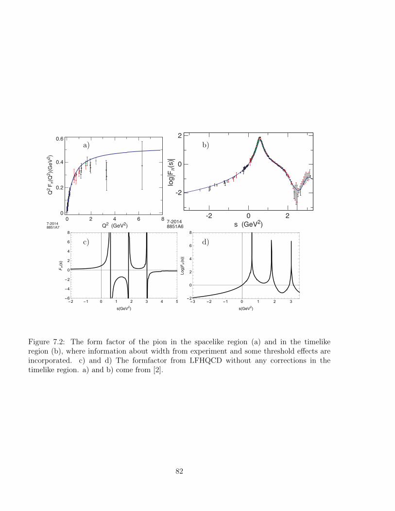
0
0.2
0.4
0.6
20 4 6 8Q2 (GeV2)
Q2
Fπ(
Q2 )
(GeV
2 )
7-20148851A7
2
0
0s (GeV2)
log
Fπ(
s)
-2 2
-2
7-20148851A6
a) b)
c) d)
Figure 7.2: The form factor of the pion in the spacelike region (a) and in the timelikeregion (b), where information about width from experiment and some threshold effects areincorporated. c) and d) The formfactor from LFHQCD without any corrections in thetimelike region. a) and b) come from [2].
82
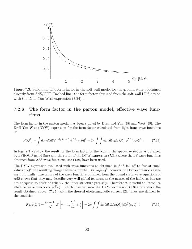
1 2 3 4 5
0.2
0.4
0.6
0.8
1
Q2 [GeV2]
F (Q2)
Figure 7.3: Solid line: The form factor in the soft wall model for the ground state , obtaineddirectly from AdS/CFT. Dashed line: the form factor obtained from the soft-wall LF functionwith the Drell-Yan West expression (7.34) .
7.2.6 The form factor in the parton model, effective wave func-tions
The form factor in the parton model has been studied by Drell and Yan [48] and West [49]. TheDrell-Yan West (DYW) expression for the form factor calculated from light front wave functionsis:
F (Q2) =
∫dx bdbdθeix|~q⊥|b cos θ|φLF (x, b)|2 = 2π
∫ ∫dx bdbJ0(xQb)|φLF (x, b)|2. (7.34)
In Fig. 7.3 we show the result for the form factor of the pion in the space-like region as obtainedby LFHQCD (solid line) and the result of the DYW expression (7.34) where the LF wave functionsobtained from AdS wave functions, see (4.9), have been used.
The DYW expression evaluated with wave functions as obtained in AdS fall off to fast at smallvalues of Q2, the resulting charge radius is infinite. For large Q2, however, the two expressions agreeasymptotically. The failure of the wave functions obtained from the bound state wave equations ofAdS shows that they may describe very well global features, as the masses of the hadrons, but arenot adequate to describe reliably the inner structure precisely. Therefore it is useful to introduceeffective wave functions φeff (ζ), which inserted into the DYW expression (7.34) reproduce theresult obtained above, (7.25), with the dressed electromagnetic current [2]. They are defined bythe condition:
FAdS(Q2) =(τ − 1)
N B
[τ − 1,
Q2
4λ+ 1
2
]= 2π
∫ ∫dx bdbJ0(xQb) |φeff
τ (x, b)|2. (7.35)
.
83
7.3 Nucleon Form Factors
7.3.1 Form factors for spin 12 fields in AdS/CFT
The coupling of the electromagnetic field to fermions is in AdS given analogously to (7.1) by:∫d4x dz
√g ΨP ′(x, z) e
MA ΓAAM (x, z)ΨP (x, z) (7.36)
The notation is the same as in sect. 4.4, below (4.30). It leads in the 4-dim space to the Diracform factor F1.
(2π)4δ4(P ′− P − q
)εµ u(P ′)γµF1(q2)u(P ), (7.37)
In the parton model it is the spin-conserving matrix element of the quark current Jµ =∑
q eq qγµq.
In AdS5 nucleons have positive and negative chirality components, Ψ+ and Ψ−, as described in sect.4.4. The spin non-flip nucleon elastic form factor F1 (Dirac form factor) is diagonal in chirality andfollows from (7.36):
FN1 (Q2) =∑±gN±
∫dz
z4J(Q2, z) Ψ2
±(z). (7.38)
The current is given by (7.13),but the same pole shift as in (7.25) will be performed. Notice thatthere is an additional scaling power in (7.38), as compared with (7.16)).
The effective charges gN± have to be determined by the specific spin-flavor structure which is notcontained in the holographic principle. For example, in the SU(6) symmetry approximation theeffective charges are computed by the sum of the charges of the struck quark convoluted by thecorresponding probability for the L = 0 and L = 1 components Ψ+ and Ψ− respectively. The resultis [2]
gp+ = 1, gp− = 0, gn+ = −1
3, gn− =
1
3. (7.39)
Since the structure of (7.36) can only account for F1, one should include an effective gauge-invariantinteraction in the five-dimensional gravity action to describe the spin-flip amplitude [50].∫
d4x dz√g ΨP ′(x, z) e
MA eNB
[ΓA,ΓB
]FMN (x, z) ΨP (x, z) (7.40)
where the resulting expression in 4 dimensions is the Pauli form factor F2.
(2π)4δ4(P ′− P − q
)εµu(P ′)
σµνqν2MN
F2(q2)u(P ) (7.41)
It corresponds to the spin-flip matrix element. Since (7.40) represents an effective interaction, itsoverall strength has to be fitted to the observed static values of the anomalous magnetic momentsχp and χn [2, 50].
Extracting the factor (2π)4δ4 (P ′− P − q) from momentum conservation in (7.41) we find [50]
FN2 (Q2) = χN
∫dz
z3Ψ+(z) J(Q2, z) Ψ−(z), (7.42)
84
where N = p, n.
Since Ψ+(z) ∼ zτ+12 and Ψ−(z) ∼ zτ+1+
12 the total power of z in the Pauli form factor (7.42) is
z2(τ+1)−3, that is F2 is a form factor with twist τ + 1.
7.3.2 A Simple Light-Front Holographic Model for Nucleon FormFactors
From (4.44) follows for the behaviour of the positive and negative component of the nucleon fieldin the ground state, note that T = J − 1
2 = 0 for the nucleon:
Ψ+(P, z) ∼ z2+12 ; Ψ−(P, z) ∼ z3+
12 (7.43)
The additional factor z12 compensates the additional power of z in (7.38) and we obtain the same
expression as for a meson. But we expect for the leading twist, L = 0, the value τ = 3 since thebaryon has 3 constituents. The discrepancy has the following reason: The wave functions derivedin sect. 4.4 are wave function of a two body system consisting of a quark and a two-quark cluster.Since the electromagnetic field interacts with both components of the cluster separately, the latterhas for the form factor to be resolved and this gives the additional factor z in the wave function.This fact corroborates our statement made in sect 7.2.6 that the bound state wave functions of AdSdescribe only the collective properties. We use the realistic twist for the nucleon wave functionsand therefore put:
Ψ+ = z12 Φ3(z) = z
12
√2
λ(λz2)3/2 (7.44)
Ψ− = z12 Φ4(z) = z
12
√2
2λ(λz2)2 (7.45)
Analogous to the pion we will consider the case where we only include the valence contribution(with probability 1 − P ) and possibly a contribution with two more constituents (pion cloud),probability P , that is in leading twist τ = 3, 5 for Ψ+. For Ψ− no higher twist is asked for by thedata.
We obtain for the proton
F p1 (Q2) = (1− P 1p )F (τ=3)(Q2) + P 1
pF(τ=5)(Q2) (7.46)
F p2 (Q2) = χp[(1− P 2p )F (τ=4)(Q2) + P 2
pF(τ=6)(Q2)] (7.47)
where χp = µp − 1 = 1.793 is the proton anomalous moment.
The valence contribution alone gives a good description of the proton Dirac form factor, see Fig.7.4, blue line, that is P 1
p ≈ 0, but the fit for the Pauli form factor can be improved by choosinga rather large higher-Fock-state probability, P 2
p ≈ 0.27, see Fig. 7.5, blue line. It is of course notsatisfactory to have different cloud contributions for the same particle, but it necessary to havegood agreement with the data.
85
It turns out that for the neutron higher twist contributions cannot ameliorate the agreement withthe experiment and we use
Fn1 (Q2) = −1
3(1− P 1
n)[F (τ=3)(Q2)− F (τ=4)(Q2)
](7.48)
−1
3P 1n
[F (τ=5)(Q2)− F (τ=6)(Q2)
](7.49)
Fn2 (Q2) = χn
[(1− γn)F (τ=4)(Q2) + γnF
(τ=6)(Q2)]
(7.50)
with the experimental value χn = µn = −1.913.
The result for the neutron Dirac form factor comes out by a constant factor 2.1 to small,see Fig.7.4, yellow line. One expects indeed that the theory is less reliable for the neutron than for theproton, since the result for the neutron form factor is the difference of two two theoretical curveswhich compensate exactly at Q2 = 0. Therefore the neutron is much more sensitive to uncertaintiesof the theory, notably to the determination of the effective charges from SU(6) symmetry.
The result for the neutron Pauli form factor is not a difference of two theoretical curves andindeed quite satisfactory, see Fig. 7.5, green line, though also here a rather large higher Fock-stateprobability has to be assumed, P 2
n = 0.38.
86

Figure 7.4: Polarization measurements and predictions for the proton and neutron Diracform factors. The blue line is the prediction of the proton Dirac form factor from LFHQCD,(7.46) with P 1
p = 0, multiplied by Q4. The orange line is the predictions for the neutronDirac form factor, Q4F n
1 (Q2) with P 1n = 0, from (7.48). The green line is the prediction
multiplied by a factor 2.1. The dotted lines are the asymptotic values, from [6].
87
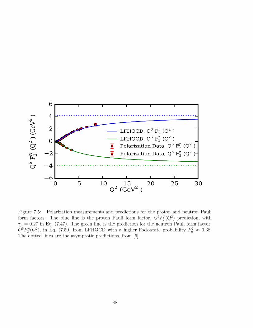
Figure 7.5: Polarization measurements and predictions for the proton and neutron Pauliform factors. The blue line is the proton Pauli form factor, Q6F p
2 (Q2) prediction, withγp = 0.27 in Eq. (7.47). The green line is the prediction for the neutron Pauli form factor,Q6F n
2 (Q2), in Eq. (7.50) from LFHQCD with a higher Fock-state probability P 2n ≈ 0.38.
The dotted lines are the asymptotic predictions, from [6].
88
7.4 Summary
LFHQCD yields a very simple and elegant analytical formula for form-factors of light hadrons inthe space-like region as well as in the time-like region. The Form factor is a Euler function whichis determined by the twist, see (7.25). To arrive at this formula from the originally derived one,(7.20) a shift from the argument Q2 + 1 in (7.20) to Q2 + 1
2 in (7.25) has to be performed.
The structure of hadron form factors is very well described by this analytical formula. In orderto have quantitative agreement with experiments additional parameters have to be introduced, asthe probability of a higher Fock state, containing an additional meson. For the neutron Dirac formfactor a strong deviation from SU(6) wave functions has to be parameterized by a multiplicativefactor, since LFHQCD cannot make predictions for the spin-isospin structure of the the nucleon.
89
Acknowledgement
One of the authors (HGD) wants to thank the Institute of Modern Physics and the LanzhouUniversity for the warm hospitality and support, he also is greatly indebted to Guy de Teramondand Stan Brodsky for countless instructive discussions. Our special thanks are also due to Prof.Zhang Pengming, who initiated this lecture, for many fruitful discussions and suggestions.
90
Appendix A
Collection of wave functions
We use different forms of wave functions, depending on the treated problem.
A.1 Mesons
For hadron wave functions we regard only such solutions which are normalizable and regular atz = 0. This implies that the spectrum has discrete values given by (4.20). The solutions Φ of theEuler-Lagrange equation (4.14) derived directly from the action (4.12) are
ΦnLAdS (z) = z2+LAdS−JL(LAdS)n (|λ|z2)e−(|λ|+λ)z2/2 (A.1)
they are normalized as: ∫ ∞0
dz eλz2z2J−3ΦnLAdS (z)2 = 1 (A.2)
L`n(x) are the associated Laguerre polynomials.
By the rescaling (4.16) we obtain solutions φ of a Schrodinger-like equqtion (4.17) which are:
φnLAdS (z) = 1/N zLAdS+1/2LLAdSn (|λ|z2)e−|λ|z2/2 with N =
√(n+ L)!
2n!|λ|−(L+1)/2 (A.3)
They are normalized to∫∞
0 dz (φnLAdS (z))2 = 1
The light front wave functions φLF are solutions of the two dimensional LF Hamiltonian (5.19) formassless constituents. They are related to the Schrodinger like wave functions by (4.9):
φLF (x, b⊥) =
√x(1− x)
2πζφ(ζ). (A.4)
and are normalized to ∫ ∞0
dx
∫d2b⊥|φLF [x, b⊥]|2 = 1 (A.5)
where ζ =√x(1− x) b⊥.
91
For the form factor it is convenient to introduce the twist wave functions Φτ by
Φτ (z) = e−λz2/2Φ(z) (A.6)
in order to compensate the factor eλz2
in the interaction action (7.1).
A.2 Baryons
For baryons the Euler Lagrange equation (4.32) can be brought into the form (4.21) with thepositive and negative chirality solutions, which are regular and normalizable:
ψ+nL(q, z) = φnL(z), ψ−nL(q, z) = φnL+1(z) (A.7)
The solutions of (4.32) are (4.36))
Ψ+(z) = z2+L+1/2−TL(L)n (|λ|z2)e−|λ|z
2/2 (A.8)
Ψ−(z) = z3+L+1/2−TL(L+1)n (|λ|z2)e−|λ|z
2/2
where T = J − 12 .
A.3 Currents
Here we look for solutions opf the Euler Lagrange equations (6.23) which are defined for any valueof q2 but vanish for z →∞. Such a solution is:
Φ(q, z) = ρ(z)U(aλ, L+ 1, |λ|z2
)(A.9)
with ρ(z) = zL−J+2e−(|λ|+λ)z2/2.
The constant aλ depends on the sign of λ:
λ < 0 aλ = − q2
4|λ| −λ
4|λ|(4− 2J + 2L)
= − q2
4|λ| +1
4(4− 2J + 2L) (A.10)
λ > 0 aλ = − q2
4|λ| −λ
4|λ|(4− 2J + 2L) + (L+ 1)
= − q2
4|λ| +1
4(2J + 2L) (A.11)
U(a, b, x) is Kummers hypergeometric function.
92
Bibliography
[1] S. J. Brodsky and G. F. de Teramond, Light-front hadron dynamics and AdS/CFT correspon-dence, Phys. Lett. B 582, 211 (2004) [arXiv:hep-th/0310227].
[2] S. J. Brodsky, G. F. de Teramond, H. G. Dosch and J. Erlich, Light-front holographic QCDand emerging confinement, Phys. Rept. 584, 1 (2015) [arXiv:1407.8131[hep-ph]].
[3] J. M. Maldacena, The large N limit of superconformal field theories and supergravity, Int. J.Theor. Phys. 38, 1113 (1999) [arXiv:hep-th/9711200].
[4] H. G. Dosch, G. F. deTeramond and S. J. Brodsky, Superconformal baryonmeson symmetryand light-front holographic QCD, Phys. Rev. D 91, 085016 (2015) [arXiv:1501.00959 [hep-th]].
[5] S. J. Brodsky and G. F. de Teramond, “Light-Front Dynamics and AdS/QCD Correspondence:The Pion Form Factor in the Space- and Time-Like Regions,” Phys. Rev. D 77 (2008) 056007,doi:10.1103/PhysRevD.77.056007 [arXiv:0707.3859 [hep-ph]].
[6] R. S. Sufian, G. F. de Teramond, S. J. Brodsky, A. Deur and H. G. Dosch, “Analysis of nucleonelectromagnetic form factors from light-front holographic QCD : The spacelike region,” Phys.Rev. D 95.014011(2017) [arXiv:1609.06688 [hep-ph]].
[7] G. ’t Hooft, “A Planar Diagram Theory for Strong Interactions,” Nucl. Phys. B 72 (1974)461, doi:10.1016/0550-3213(74)90154-0.
[8] G. Veneziano, Nuovo Cim. A 57 (1968) 190, doi:10.1007/BF02824451.
[9] S. S. Gubser, I. R. Klebanov and A. M. Polyakov, Gauge theory correlators from non-criticalstring theory, Phys. Lett. B 428, 105 (1998) [arXiv:hep-th/9802109].
[10] E. Witten, Anti-de Sitter space and holography, Adv. Theor. Math. Phys. 2, 253 (1998)[arXiv:hep-th/9802150].
[11] A.V. Ramallo, Introduction to the AdS/CFT correspondence, Springer Proc. Phys. 161 (2015)411 [arXiv:1310.4319 [hep-th]].
[12] M. Ammon and J. Erdmenger, Gauge/Gravity Duality: Foundations and Applications, Cam-bridge University Press, (2015).
[13] S. S. Gubser and A. Karch, “From gauge-string duality to strong interactions: A Pedestrian’sGuide,” Ann. Rev. Nucl. Part. Sci. 59 (2009) 145, doi:10.1146/annurev.nucl.010909.083602[arXiv:0901.0935 [hep-th]].
93
[14] I. R. Klebanov and J. M. Maldacena, Phys. Today 62 (2009) 28, doi:10.1063/1.3074260.
[15] A. V. Manohar, “Large N QCD,” hep-ph/9802419.
[16] J. Erlich, E. Katz, D. T. Son and M. A. Stephanov, QCD and a holographic model of hadrons,Phys. Rev. Lett. 95, 261602 (2005) [arXiv:hep-ph/0501128].
[17] S. J. Brodsky and G. F. de Teramond, Hadronic spectra and lightfront wavefunctions inholographic QCD, Phys. Rev. Lett. 96 (2006) 201601, doi:10.1103/PhysRevLett.96.201601[arXiv:hep-ph/0602252].
[18] A. Karch, E. Katz, D. T. Son and M. A. Stephanov, Linear confinement and AdS/QCD, Phys.Rev. D 74, 015005 (2006) [arXiv:hep-ph/0602229].
[19] P. A. M. Dirac, Forms of relativistic dynamics, Rev. Mod. Phys. 21, 392 (1949).
[20] S. J. Brodsky, H. C. Pauli and S. S. Pinsky, Quantum chromodynamics and other field theorieson the light cone, Phys. Rept. 301, 299 (1998) [arXiv:hep-ph/9705477].
[21] G. F. de Teramond, H. G. Dosch and S. J. Brodsky, Kinematical and dynamical aspectsof higher-spin bound-state equations in holographic QCD, Phys. Rev. D 87, 075005 (2013)[arXiv:1301.1651 [hep-ph]].
[22] W. Rarita and J. Schwinger, On a theory of particles with half integral spin, Phys. 8Rev. 60,61 (1941).
[23] I. Kirsch, Spectroscopy of fermionic operators in AdS/CFT, JHEP 0609, 052 (2006) [arXiv:hep-th/0607205].
[24] G. F. de Teramond, H. G. Dosch and S. J. Brodsky, Baryon spectrum from superconformalquantum mechanics and its light-front holographic embedding, Phys. Rev. D 91, 045040 (2015)[arXiv:1411.5243 [hep-ph]].
[25] H. G. Dosch, G. F. de Teramond and S. J. Brodsky, Supersymmetry across the light andheavy-light hadronic spectrum, Phys. Rev. D 92, 074010 (2015) [arXiv:1504.05112 [hep-ph]].
[26] H. G. Dosch, G. F. de Teramond and S. J. Brodsky, Supersymmetry Across the Light andHeavy-Light Hadronic Spectrum II, Phys. Rev. D.95.034016(2017) [arXiv:1612.02370 [hep-ph]].
[27] S. J. Brodsky, G. F. de T eramond, H. G. Dosch and C. Lorc e, Universal effective hadrondynamics from superconformal algebra, Phys. Lett. B 759, 171 (2016) [arXiv:1604.06746 [hep-ph]].
[28] V. de Alfaro, S. Fubini and G. Furlan, Conformal invariance in quantum mechanics, NuovoCim. A 34, 569 (1976).
[29] E. Witten, Dynamical breaking of supersymmetry, Nucl. Phys. B 188, 513 (1981).
[30] V. P. Akulov and A. I. Pashnev, Quantum superconformal model in (1,2) space, Theor. Math.Phys. 56, 862 (1983) [Teor. Mat. Fiz. 56, 344 (1983)].
[31] S. Fubini and E. Rabinovici, Superconformal quantum mechanics, Nucl. Phys. B 245, 17 (1984).
94
[32] R. Van Royen and V. F.Weisskopf, Hadron decay processes and the quark model, Nuovo Cim.A 50 617 (1967).
[33] E. V. Shuryak, Hadrons containing a heavy quark and QCD sum rules, Nucl. Phys. B 198, 83(1982).
[34] N. Isgur and M. B. Wise, Spectroscopy with heavy quark symmetry, Phys. Rev. Lett. 66 (1991)1130.
[35] R. Aaij et al. [LHCb Collaboration], “Observation of the doubly charmed baryon Ξ++cc ,”
[arXiv:1707.01621 [hep-ex]].
[36] M. Karliner and J. L. Rosner, “Discovery of doubly-charmed Xicc s baryon implies a stable(b b ubar dbar) tetraquark,” [arXiv:1707.07666 [hep-ph]].
[37] M. A. Shifman, A. I. Vainshtein and V. I. Zakharov, Nucl. Phys. B 147 (1979) 385,doi:10.1016/0550-3213(79)90022-1.
[38] M. Abramowitz and I. A. Stegun, ”Pocketbook of Mathematical Functions”, NBS, 1964,abridged version,1984.
[39] F. Jugeau, S. Narison and H. Ratsimbarison, Phys. Lett. B 722 (2013) 111,doi:10.1016/j.physletb.2013.04.008 [arXiv:1302.6909 [hep-ph]].
[40] P. Colangelo, F. De Fazio, F. Giannuzzi, F. Jugeau and S. Nicotri, Phys. Rev. D 78 (2008)055009 doi:10.1103/PhysRevD.78.055009, [arXiv:0807.1054 [hep-ph]].
[41] J. Erlich, G. D. Kribs and I. Low, Phys. Rev. D 73 (2006) 096001,doi:10.1103/PhysRevD.73.096001 [arXiv:hep-th/0602110].
[42] A. A. Migdal, “Multicolor QCD as dual resonance theory,” Annals Phys. 109, 365 (1977).
[43] G. F. de Teramond and S. J. Brodsky, “Hadronic form factor models and spectroscopy withinthe gauge/gravity correspondence” [arXiv:1203.4025 [hep-ph]].
[44] J. Polchinski and M. J. Strassler, “Deep inelastic scattering and gauge/string duality,” JHEP0305, 012 (2003) [arXiv:hep-th/0209211].
[45] J. Polchinski and M. J. Strassler, Phys. Rev. Lett. 88 (2002) 031601,doi:10.1103/PhysRevLett.88.031601, [hep-th/0109174].
[46] S. J. Brodsky and G. R. Farrar, Phys. Rev. Lett. 31 (1973) 1153.
[47] S. J. Brodsky and G. R. Farrar, “Scaling Laws for Large Momentum Transfer Processes,”Phys. Rev. D 11 (1975) 1309.
[48] S. D. Drell and T. M. Yan, “Connection of elastic electromagnetic nucleon form-factors atlarge Q2 and deep inelastic structure functions near threshold,” Phys. Rev. Lett. 24, 181(1970).
[49] G. B. West, “Phenomenological model for the electromagnetic structure of the proton,” Phys.Rev. Lett. 24, 1206 (1970).
95

[50] Z. Abidin and C. E. Carlson, “Nucleon electromagnetic and gravitational form fac-tors from holography,” Phys. Rev. D 79 (2009) 115003, doi:10.1103/PhysRevD.79.115003[arXiv:0903.4818 [hep-ph]].
96