Embed Size (px)
Citation preview

A UNIFIED APPROACH TO MIXED-INTEGER OPTIMIZATIONPROBLEMS WITH LOGICAL CONSTRAINTS
DIMITRIS BERTSIMAS∗, RYAN CORY-WRIGHT† , AND JEAN PAUPHILET‡
Abstract. We propose a unified framework to address a family of classical mixed-integer op-timization problems with logically constrained decision variables, including network design, facilitylocation, unit commitment, sparse portfolio selection, binary quadratic optimization, sparse princi-pal component analysis, and sparse learning problems. These problems exhibit logical relationshipsbetween continuous and discrete variables, which are usually reformulated linearly using a big-Mformulation. In this work, we challenge this longstanding modeling practice and express the logi-cal constraints in a non-linear way. By imposing a regularization condition, we reformulate theseproblems as convex binary optimization problems, which are solvable using an outer-approximationprocedure. In numerical experiments, we establish that a general-purpose numerical strategy, whichcombines cutting-plane, first-order, and local search methods, solves these problems faster and at alarger scale than state-of-the-art mixed-integer linear or second-order cone methods. Our approachsuccessfully solves network design problems with 100s of nodes and provides solutions up to 40%better than the state-of-the-art; sparse portfolio selection problems with up to 3, 200 securities com-pared with 400 securities for previous attempts; and sparse regression problems with up to 100, 000covariates.
Key words. mixed-integer optimization; branch and cut; outer approximation
AMS subject classifications. 90C11, 90C57, 90C90
1. Introduction. Many important problems from the Operations Research lit-erature exhibit a logical relationship between continuous variables x and binary vari-ables z of the form “x = 0 if z = 0”. Among others, start-up costs in machine sched-uling problems, financial transaction costs, cardinality constraints and fixed costs infacility location problems exhibit this relationship. Since the work of [34], this rela-tionship is usually enforced through a “big-M” constraint of the form −Mz ≤ x ≤Mzfor a sufficiently large constant M > 0. Glover’s work has been so influential thatbig-M constraints are now considered as intrinsic components of the initial problemformulations themselves, to the extent that textbooks in the field introduce facility lo-cation, network design or sparse portfolio problems with big-M constraints by default,although they are actually reformulations of logical constraints.
In this work, we adopt a different perspective on the big-M paradigm, view-ing it as a regularization term, rather than a modeling trick. Under this lens, weshow that regularization drives the computational tractability of problems with log-ical constraints, explore alternatives to the big-M paradigm and propose an efficientalgorithmic strategy which solves a broad class of problems with logical constraints.
1.1. Problem Formulation and Main Contributions. We consider opti-mization problems which unfold over two stages. In the first stage, a decision-makeractivates binary variables, while satisfying resource budget constraints and incurringactivation costs. Subsequently, in the second stage, the decision-maker optimizes overthe continuous variables. Formally, we consider the problem
(1.1) minz∈Z,x∈Rn
c>z + g(x) + Ω(x) s.t. xi = 0 if zi = 0 ∀i ∈ [n],
∗Sloan School of Management, Massachusetts Institute of Technology, Cambridge, MA, USA([email protected]).†Operations Research Center, Massachusetts Institute of Technology, Cambridge, MA, USA
([email protected]).‡London Business School, London, UK ([email protected]).
1
arX
iv:1
907.
0210
9v3
[m
ath.
OC
] 2
5 Ja
n 20
21

2 D. BERTSIMAS, R. CORY-WRIGHT, AND J. PAUPHILET
where Z ⊆ 0, 1n, c ∈ Rn is a cost vector, g(·) is a generic convex function whichpossibly models convex constraints x ∈ X for a convex set X ⊆ Rn implicitly—byrequiring that g(x) = +∞ if x /∈ X , and Ω(·) is a convex regularization function; weformally state its structure in Assumption 2.2.
In this paper, we provide three main contributions: First, we reformulate thelogical constraint “xi = 0 if zi = 0” in a non-linear way, by substituting zixi for xi inProblem (1.1). Second, we leverage the regularization term Ω(x) to derive a tractablereformulation of (1.1). Finally, by invoking strong duality, we reformulate (1.1) as amixed-integer saddle-point problem, which is solvable via outer approximation.
Observe that the structure of Problem (1.1) is quite general, as the feasible set Zcan capture known lower and upper bounds on z, relationships between different zi’s,or a cardinality constraint e>z ≤ k. Moreover, constraints of the form x ∈ X , forsome convex set X , can be encoded within the domain of g, by defining g(x) = +∞ ifx /∈ X . As a result, Problem (1.1) encompasses a large number of problems from theOperations Research literature, such as the network design problem described in Ex-ample 1.1. These problems are typically studied separately. However, the techniquesdeveloped for each problem are actually different facets of a single unified story, and,as we demonstrate in this paper, can be applied to a much more general class ofproblems than is often appreciated.
Example 1.1. Network design is an important example of problems of theform (1.1). Given a set of m nodes, the network design problem consists ofconstructing edges to minimize the construction plus flow transportation cost.Let E denote the set of all potential edges and let n = |E|. Then, the networkdesign problem is given by:
(1.2)min
z∈Z,x∈Rn+
c>z + 12x>Qx+ d>x s.t. Ax = b,
xe = 0 if ze = 0 ∀e ∈ E,
where Z = 0, 1n, A ∈ Rm×n is the flow conservation matrix, b ∈ Rm is thevector of external demands and Q ∈ Rn×n, d ∈ Rn define the quadratic andlinear costs of flow circulation. We assume that Q 0 is a positive semidefinitematrix. Inequalities of the form ` ≤ z ≤ u can be incorporated within Z toaccount for existing/forbidden edges in the network. Problem (1.2) is of thesame form as Problem (1.1) with
g(x) + Ω(x) :=
12x>Qx+ d>x, if Ax = b,x ≥ 0,
+∞, otherwise.
We present a generalized model with edge capacities and multiple commodities inSection 2.1.1.
1.2. Background and Literature Review. Our work falls into two areas ofthe mixed-integer optimization literature which are often considered in isolation: (a)modeling forcing constraints which encode whether continuous variables are activeand can take non-zero values or are inactive and forced to 0, and (b) decompositionalgorithms for mixed-integer optimization problems.
A UNIFIED APPROACH TO MIXED-INTEGER OPTIMIZATION 3
Formulations of forcing constraints. The most popular way to impose forc-ing constraints on continuous variables is to introduce auxiliary discrete variableswhich encode whether the continuous variables are active, and relate the discrete andcontinuous variables via the big-M approach of [34]. This approach was first appliedto mixed-integer non-linear optimization (MINLO) in the context of sparse portfolioselection by [14]. With the big-M approach, the original MINLO admits boundedrelaxations and can therefore be solved via branch-and-bound. Moreover, becausethe relationship between discrete and continuous variables is enforced via linear con-straints, a big-M reformulation has a theoretically low impact on the tractability ofthe MINLOs continuous relaxations. However, in practice, high values of M lead tonumerical instability and provide low-quality bounds [see 4, Section 5].
This observation led [28] to propose a class of cutting-planes for MINLO prob-lems with indicator variables, called perspective cuts, which often provide a tighterreformulation of the logical constraints. Their approach was subsequently extendedby [1], who, building upon the work of [5, pp. 88, item 5], proved that MINLO prob-lems with indicator variables can often be reformulated as mixed-integer second-ordercone problems (see [37] for a survey). More recently, a third approach for couplingthe discrete and the continuous in MINLO was proposed independently for sparseregression by [47] and [13]: augmenting the objective with a strongly convex term ofthe form ‖x‖22, called a ridge regularizer.
In the present paper, we synthesize the aforementioned and seemingly unrelatedthree lines of research under the unifying lens of regularization. Notably, our frame-work includes big-M and ridge regularization as special cases, and provides an ele-mentary derivation of perspective cuts.
Numerical algorithms for mixed-integer optimization. A variety of “clas-sical” general-purpose decomposition algorithms have been proposed for general MIN-LOs. The first such decomposition method is known as Generalized Benders Decom-position, and was proposed by [33] as an extension of [6]. A similar method, knownas outer-approximation was proposed by [22], who proved its finite termination. Theouter-approximation method was subsequently generalized to account for non-linearintegral variables by [25]. These techniques decompose MINLOs into a discrete mas-ter problem and a sequence of continuous separation problems, which are iterativelysolved to generate valid cuts for the master problem.
Though slow in their original implementation, decomposition schemes have ben-efited from recent improvements in mixed-integer linear solvers in the past decades,beginning with the branch-and-cut approaches of [45, 48], which embed the cut gen-eration process within a single branch-and-bound tree, rather than building a branch-and-bound tree before generating each cut. We refer to [23, 24] for recent successfulimplementations of “modern” decomposition schemes. From a high-level perspective,these recent successes require three key ingredients: First, a fast cut generation strat-egy. Second, as advocated by [23], a rich cut generation process at the root node.Finally, a cut selection rule for degenerate cases where multiple valid inequalities exist(e.g., the Pareto optimality criteria of [43]).
In this paper, we connect the regularization used to reformulate logical constraintswith the aforementioned key ingredients for modern decomposition schemes. Hence,instead of considering a MINLO formulation as a given and subsequently attempt tosolve it at scale, our approach view big-M constraints as one of many alternatives.We argue that regularization is a modeling choice that impacts the tractability of theformulation and should be made accordingly.

4 D. BERTSIMAS, R. CORY-WRIGHT, AND J. PAUPHILET
1.3. Structure. We propose a unifying framework to address mixed-integer op-timization problems, and jointly discuss modeling choice and numerical algorithms.
In Section 2, we identify a general class of mixed-integer optimization problems,which encompasses sparse regression, sparse portfolio selection, sparse principal com-ponent analysis, unit commitment, facility location, network design and binary qua-dratic optimization as special cases. For this class of problems, we discuss how impos-ing either big-M or ridge regularization accounts for non-linear relationships betweencontinuous and binary variables in a tractable fashion. We also establish that regular-ization controls the convexity and smoothness of Problem (1.1)’s objective function.
In Section 3, we propose a conjunction of general-purpose numerical algorithmsto solve Problem (1.1). The backbone of our approach is an outer approximationframework, enhanced with first-order methods to solve the Boolean relaxations andobtain improved lower bounds, certifiably near-optimal warm-starts via randomizedrounding, and a discrete local search procedure. We also connect our approach to theperspective cut approach [28] from a theoretical and implementation standpoint.
Finally, in Section 4, we demonstrate empirically that algorithms derived fromour framework can outperform state-of-the-art solvers. On network design problemswith 100s of nodes and binary quadratic optimization problems with 100s of vari-ables, we improve the objective value of the returned solution by 5 to 40% and 5to 85% respectively, and our edge increases as the problem size increases. On em-pirical risk minimization problems, our method with ridge regularization is able toaccurately select features among 100, 000s (resp. 10, 000s) of covariates for regression(resp. classification) problems, with higher accuracy than both Lasso and non-convexpenalties from the statistics literature. For sparse portfolio selection, we solve toprovable optimality problems one order of magnitude larger than previous attempts.We then analyze the benefits of the different ingredients in our numerical recipe onfacility location problems, and discuss the relative merits of different regularizationapproaches on unit commitment instances.
Notation. We use nonbold face characters to denote scalars and components ofmatrices, lowercase bold faced characters such as x to denote vectors, uppercase boldfaced characters such as X to denote matrices, and calligraphic characters such as Xto denote sets. We let e denote a vector of all 1’s, and 0 denote a vector of all 0’s,with dimension implied by the context. If x is a n-dimensional vector then Diag(x)denotes the n × n diagonal matrix whose diagonal entries are given by x. If f(x) isa convex function then its perspective function ϕ(x, t), defined as ϕ(x, t) = tf(x/t)if t > 0, ϕ(0, 0) = 0, and ∞ elsewhere, is also convex [17, Chapter 3.2.6.]. Finally, welet Rn+ denote the n-dimensional nonnegative orthant.
2. Framework and Examples. In this section, we present the family of prob-lems to which our analysis applies, discuss the role played by regularization, andprovide some examples from the Operations Research literature.
2.1. Examples. Problem (1.1) has a two-stage structure which comprises first“turning on” some indicator variables z, and second solving a continuous optimizationproblem over the active components of x. Precisely, Problem (1.1) can be viewed asa discrete optimization problem:
minz∈Z
c>z + f(z),(2.1)
where the inner minimization problem
(2.2) f(z) := minx∈Rn
g(x) + Ω(x) s.t. xi = 0 if zi = 0 ∀i ∈ [n],
A UNIFIED APPROACH TO MIXED-INTEGER OPTIMIZATION 5
yields a best choice of x given z. As we illustrate in this section, a number of problemsof practical interest exhibit this structure.
Example 2.1. For the network design example (1.2), we have
f(z) := minx∈Rn
+:Ax=b
12x>Qx+ d>x s.t. xe = 0 if ze = 0 ∀e ∈ E.
2.1.1. Network Design. Example 1.1 illustrates that the single-commoditynetwork design problem is a special case of Problem (1.1). We now formulate thek-commodity network design problem with directed capacities as minimizing overZ = 0, 1n the function:
(2.3)
f(z) := minfj ,x∈Rn
+
12x>Qx+ d>x s.t. Af j = bj ∀j ∈ [k],
x =
k∑j=1
f j , x ≤ u,
xe = 0 if ze = 0 ∀e ∈ E.
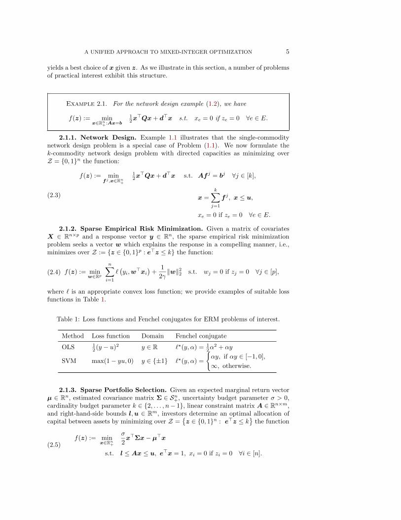
2.1.2. Sparse Empirical Risk Minimization. Given a matrix of covariatesX ∈ Rn×p and a response vector y ∈ Rn, the sparse empirical risk minimizationproblem seeks a vector w which explains the response in a compelling manner, i.e.,minimizes over Z := z ∈ 0, 1p : e>z ≤ k the function:
(2.4) f(z) := minw∈Rp
n∑i=1
`(yi,w
>xi)
+1
2γ‖w‖22 s.t. wj = 0 if zj = 0 ∀j ∈ [p],
where ` is an appropriate convex loss function; we provide examples of suitable lossfunctions in Table 1.
Table 1: Loss functions and Fenchel conjugates for ERM problems of interest.
Method Loss function Domain Fenchel conjugate
OLS 12 (y − u)2 y ∈ R `?(y, α) = 1
2α2 + αy
SVM max(1− yu, 0) y ∈ ±1 `?(y, α) =
αy, if αy ∈ [−1, 0],
∞, otherwise.
2.1.3. Sparse Portfolio Selection. Given an expected marginal return vectorµ ∈ Rn, estimated covariance matrix Σ ∈ Sn+, uncertainty budget parameter σ > 0,cardinality budget parameter k ∈ 2, . . . , n− 1, linear constraint matrix A ∈ Rn×m,and right-hand-side bounds l,u ∈ Rm, investors determine an optimal allocation ofcapital between assets by minimizing over Z =
z ∈ 0, 1n : e>z ≤ k
the function
(2.5)f(z) := min
x∈Rn+
σ
2x>Σx− µ>x
s.t. l ≤ Ax ≤ u, e>x = 1, xi = 0 if zi = 0 ∀i ∈ [n].
6 D. BERTSIMAS, R. CORY-WRIGHT, AND J. PAUPHILET
2.1.4. Unit Commitment. In the DC-load-flow unit commitment problem,each generation unit i incurs a cost given by a quadratic cost function f i(x) = aix
2 +bix+ ci for its power generation output x ∈ [0, ui]. Let T denote a finite set of timeperiods covering a time horizon (e.g., 24 hours). At each time period t ∈ T , thereis an estimated demand dt. The objective is to generate sufficient power to satisfydemand at minimum cost, while respecting minimum time on/time off constraints.
By introducing binary variables zi,t, which denote whether generation unit i isactive in time period t, requiring that z ∈ Z, i.e., z obeys physical constraints suchas minimum time on/off, the unit commitment problem admits the formulation:
minz
f(z) +∑t∈T
n∑i=1
cizi,t s.t. z ∈ Z ⊆ 0, 1n×|T |,(2.6)
(2.7)
where: f(z) := minx
∑t∈T
(n∑i=1
12aix
2i,t + bixi,t
)s.t.
n∑i=1
xi,t ≥ Dt ∀t ∈ T ,
xi,t ∈ [0, ui,t] ∀i ∈ [n],∀t ∈ T ,xi,t = 0 if zi,t = 0 ∀i ∈ [n],∀t ∈ T .
2.1.5. Facility Location. Given a set of n facilities and m customers, the fa-cility location problem consists of constructing facilities i ∈ [n] at cost ci to satisfydemand at minimal cost, i.e., minimizing over Z = 0, 1n the function:(2.8)
f(z) := minX∈Rn×m
+
c>z +
m∑j=1
n∑i=1
cijxij s.t.
m∑j=1
xij ≤ ui ∀i ∈ [n],
n∑i=1
xij = dj ∀j ∈ [m], xij = 0 if zi = 0 ∀i ∈ [n], j ∈ [m].
In this formulation, xij corresponds to the quantity produced in facility i and shippedto customer j at a marginal cost of cij . Moreover, each facility i has a maximumoutput capacity of ui and each customer j has a demand of dj . In the uncapacitatedcase where ui = ∞, the inner minimization problems decouple into independentknapsack problems for each customer j.
2.1.6. Sparse Principal Component Analysis (PCA). Given a p × p pos-itive semidefinite covariance matrix Σ, Σ ∈ Sp+ in short, the sparse PCA problem isto select a vector z which maximizes over Z =
z ∈ 0, 1p : e>z ≤ k
the function
f(z) = maxx∈Rp
x>Σx s.t. ‖x‖22 = 1, xi = 0 if zi = 0 ∀i ∈ [p].(2.9)
This function is apparently non-concave in z, because f(z) is the optimal value ofa non-convex quadratic optimization problem. Fortuitously however, this problemadmits an exact mixed-integer semidefinite reformulation, namely
f(z) = maxX∈Sp
+
〈Σ,X〉 s.t. tr(X) = 1, xi,j = 0 if zi = 0 or zj = 0 ∀i, j ∈ [p].(2.10)
Indeed, for any fixed z, Problem (2.10) maximizes a linear function inX and thereforeadmits a rank-one optimal solution. Thus, we prove that sparse PCA admits an exactmixed-integer semidefinite optimization reformulation.

A UNIFIED APPROACH TO MIXED-INTEGER OPTIMIZATION 7
2.1.7. Binary Quadratic Optimization. Given a symmetric cost matrix Q,the binary quadratic optimization problem consists of selecting a vector of binaryvariables z which minimizes over Z = 0, 1n the function:
(2.11) f(z) = z>Qz.
This formulation is non-convex and does not include continuous variables. How-ever, introducing auxiliary continuous variables yields the equivalent formulation [26]of minimizing over Z = 0, 1n the function:
f(z) := minY ∈Rn×n
+
〈Q,Y 〉 s.t. yi,j ≤ 1 ∀i, j ∈ [n],(2.12)
yi,j ≥ zi + zj − 1 ∀i ∈ [n],∀j ∈ [n]\i,yi,i ≥ zi ∀i ∈ [n],
yi,j = 0 if zi = 0 ∀i, j ∈ [n],
yi,j = 0 if zj = 0 ∀i, j ∈ [n].
2.1.8. Union of Ellipsoidal Constraints. We now demonstrate that an evenbroader class of problems than MIOs with logical constraints can be cast within ourframework. Concretely, we demonstrate that constraints x ∈ S :=
⋃ki=1(Qi ∩ Pi),
where Qi := x ∈ Rn : x>Qix + h>i x + gi ≤ 0, with Qi 0, is an ellipsoid andPi := x : Aix ≤ bi is a polytope, can be reformulated as a special case of ourframework. We remark that the constraint x ∈ S is very general. Indeed, if we wereto omit the quadratic constraints then we obtain a so-called ideal union of polyhedraformulation, which essentially all mixed-binary linear feasible regions admit [see 52].
To derive a mixed-integer formulation with logical constraints of S that fits withinour framework, we introduce xi ∈ Rn and δi ∈ 0, 1n, such that xi ∈ Qi ∩ Pi ifδi = 1, xi = 0 otherwise, and x =
∑i xi. We enforce xi ∈ Qi ∩ Pi by introducing
slack variables ξi, ρi for the linear and quadratic constraints respectively, and forcingthem to be zero whenever δi = 1. Formally, S admits the following formulation
x =
k∑i=1
xi,
k∑i=1
δi = 1,(2.13)
Aixi ≤ bi + ξi ∀i ∈ [k],
x>i Qixi + h>i xi + gi ≤ ρi ∀i ∈ [k],
xi = 0 if δi = 0 ∀i ∈ [k],
ξi = 0 if (1− δi) = 0 ∀i ∈ [k],
ρi = 0 if (1− δi) = 0 ∀i ∈ [k].
2.2. A Regularization Assumption. When we stated Problem (1.1), we as-sumed that its objective function consists of a convex function g(x) plus a regulariza-tion term Ω(x). We now formalize this assumption:
Assumption 2.2. In Problem (1.1), the regularization term Ω(x) is one of:• a big-M penalty function, Ω(x) = 0 if ‖x‖∞ ≤M and ∞ otherwise,
• a ridge penalty, Ω(x) =1
2γ‖x‖22.
This decomposition often constitutes a modeling choice in itself. We now illustratethis idea via the network design example.

8 D. BERTSIMAS, R. CORY-WRIGHT, AND J. PAUPHILET
Example 2.3. In the network design example (1.2), given the flow conser-vation structure Ax = b, we have that x ≤ Me, where M =
∑i:bi>0 bi. In
addition, if Q 0 then the objective function naturally contains a ridge reg-ularization term with 1/γ equal to the smallest eigenvalue of Q. Moreover, itis possible to obtain a tighter natural ridge regularization term by solving thefollowing auxiliary semidefinite optimization problem a priori
maxq≥0
e>q s.t. Q−Diag(q) 0,
and using qi as the ridge regularizer for each index i [30].
Big-M constraints are often considered to be a modeling trick. However, our frame-work demonstrates that imposing either big-M constraints or a ridge penalty is aregularization method, rather than a modeling trick. Interestingly, ridge regulariza-tion accounts for the relationship between the binary and continuous variables justas well as big-M regularization, without performing an algebraic reformulation of thelogical constraints1.
Conceptually, both regularization functions are equivalent to a soft or hard con-straint on the continuous variables x. However, they admit practical differences: Forbig-M regularization, there usually exists a finite value M0, typically unknown a pri-ori, such that if M < M0, the regularized problem is infeasible. Alternatively, forevery value of the ridge regularization parameter γ, if the original problem is feasiblethen the regularized problem is also feasible. Consequently, if there is no naturalchoice of M then imposing ridge regularization may be less restrictive than impos-ing big-M regularization. However, for any γ > 0, the objective of the optimizationproblem with ridge regularization is different from its unregularized limit as γ →∞,while for big-M regularization, there usually exists a finite value M1 above which thetwo objective values match. We illustrate this discussion numerically in Section 4.3.
2.3. Duality to the Rescue. In this section, we derive Problem (2.2)’s dualand reformulate f(z) as a maximization problem. This reformulation is significantfor two reasons: First, as shown in the proof of Theorem 2.5, it leverages a non-linearreformulation of the logical constraints “xi = 0 if zi = 0” by introducing additionalvariables vi such that vi = zixi. Second, it proves that the regularization term Ω(x)drives the convexity and smoothness of f(z), and thereby drives the computationaltractability of the problem. To derive Problem (2.2)’s dual, we require:
Assumption 2.4. For each subproblem generated by f(z), where z ∈ Z, eitherthe optimization problem is infeasible, or strong duality holds.
Note that all seven problems stated in Section 2.1 satisfy Assumption 2.4, astheir inner problems are convex quadratics with linear or semidefinite constraints [17,Section 5.2.3]. Under Assumption 2.4, the following theorem reformulates Problem(2.1) as a saddle-point problem:
1Specifically, ridge regularization enforces logical constraints through perspective functions, as ismade clear in Section 3.4.
A UNIFIED APPROACH TO MIXED-INTEGER OPTIMIZATION 9
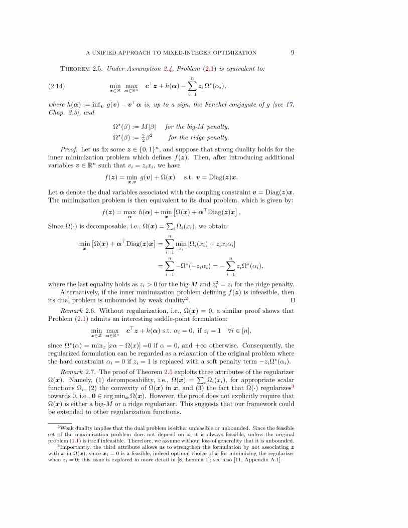
Theorem 2.5. Under Assumption 2.4, Problem (2.1) is equivalent to:
(2.14) minz∈Z
maxα∈Rn
c>z + h(α)−n∑i=1
zi Ω?(αi),
where h(α) := infv g(v) − v>α is, up to a sign, the Fenchel conjugate of g [see 17,Chap. 3.3], and
Ω?(β) := M |β| for the big-M penalty,
Ω?(β) := γ2β
2 for the ridge penalty.
Proof. Let us fix some z ∈ 0, 1n, and suppose that strong duality holds for theinner minimization problem which defines f(z). Then, after introducing additionalvariables v ∈ Rn such that vi = zixi, we have
f(z) = minx,v
g(v) + Ω(x) s.t. v = Diag(z)x.
Let α denote the dual variables associated with the coupling constraint v = Diag(z)x.The minimization problem is then equivalent to its dual problem, which is given by:
f(z) = maxα
h(α) + minx
[Ω(x) +α>Diag(z)x
],
Since Ω(·) is decomposable, i.e., Ω(x) =∑i Ωi(xi), we obtain:
minx
[Ω(x) +α>Diag(z)x
]=
n∑i=1
minxi
[Ωi(xi) + zixiαi]
=
n∑i=1
−Ω?(−ziαi) = −n∑i=1
ziΩ?(αi),
where the last equality holds as zi > 0 for the big-M and z2i = zi for the ridge penalty.Alternatively, if the inner minimization problem defining f(z) is infeasible, then
its dual problem is unbounded by weak duality2.
Remark 2.6. Without regularization, i.e., Ω(x) = 0, a similar proof shows thatProblem (2.1) admits an interesting saddle-point formulation:
minz∈Z
maxα∈Rn
c>z + h(α) s.t. αi = 0, if zi = 1 ∀i ∈ [n],
since Ω?(α) = minx [xα− Ω(x)] =0 if α = 0, and +∞ otherwise. Consequently, theregularized formulation can be regarded as a relaxation of the original problem wherethe hard constraint αi = 0 if zi = 1 is replaced with a soft penalty term −ziΩ?(αi).
Remark 2.7. The proof of Theorem 2.5 exploits three attributes of the regularizerΩ(x). Namely, (1) decomposability, i.e., Ω(x) =
∑i Ωi(xi), for appropriate scalar
functions Ωi, (2) the convexity of Ω(x) in x, and (3) the fact that Ω(·) regularizes3
towards 0, i.e., 0 ∈ arg minx Ω(x). However, the proof does not explicitly require thatΩ(x) is either a big-M or a ridge regularizer. This suggests that our framework couldbe extended to other regularization functions.
2Weak duality implies that the dual problem is either unfeasible or unbounded. Since the feasibleset of the maximization problem does not depend on z, it is always feasible, unless the originalproblem (1.1) is itself infeasible. Therefore, we assume without loss of generality that it is unbounded.
3Importantly, the third attribute allows us to strengthen the formulation by not associating zwith x in Ω(x), since xi = 0 is a feasible, indeed optimal choice of x for minimizing the regularizerwhen zi = 0; this issue is explored in more detail in [8, Lemma 1]; see also [11, Appendix A.1].
10 D. BERTSIMAS, R. CORY-WRIGHT, AND J. PAUPHILET
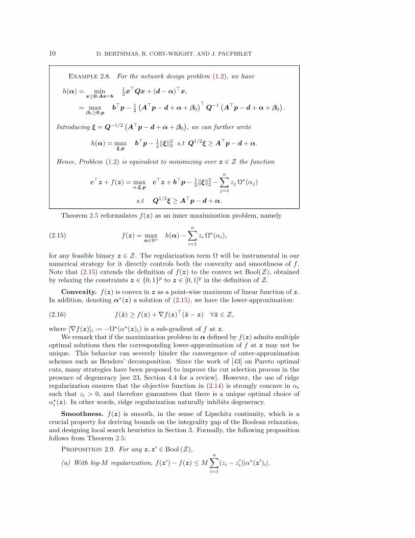
Example 2.8. For the network design problem (1.2), we have
h(α) = minx≥0:Ax=b
12x>Qx+ (d−α)>x,
= maxβ0≥0,p
b>p− 12
(A>p− d+α+ β0
)>Q−1
(A>p− d+α+ β0
).
Introducing ξ = Q−1/2(A>p− d+α+ β0
), we can further write
h(α) = maxξ,p
b>p− 12‖ξ‖
22 s.t Q1/2ξ ≥ A>p− d+α.
Hence, Problem (1.2) is equivalent to minimizing over z ∈ Z the function
c>z + f(z) = maxα,ξ,p
c>z + b>p− 12‖ξ‖
22 −
n∑j=1
zj Ω?(αj)
s.t Q1/2ξ ≥ A>p− d+α.
Theorem 2.5 reformulates f(z) as an inner maximization problem, namely
f(z) = maxα∈Rn
h(α)−n∑i=1
zi Ω?(αi),(2.15)
for any feasible binary z ∈ Z. The regularization term Ω will be instrumental in ournumerical strategy for it directly controls both the convexity and smoothness of f .Note that (2.15) extends the definition of f(z) to the convex set Bool(Z), obtainedby relaxing the constraints z ∈ 0, 1p to z ∈ [0, 1]p in the definition of Z.
Convexity. f(z) is convex in z as a point-wise maximum of linear function of z.In addition, denoting α?(z) a solution of (2.15), we have the lower-approximation:
(2.16) f(z) ≥ f(z) +∇f(z)>(z − z) ∀z ∈ Z,
where [∇f(z)]i := −Ω?(α?(z)i) is a sub-gradient of f at z.We remark that if the maximization problem in α defined by f(z) admits multiple
optimal solutions then the corresponding lower-approximation of f at z may not beunique. This behavior can severely hinder the convergence of outer-approximationschemes such as Benders’ decomposition. Since the work of [43] on Pareto optimalcuts, many strategies have been proposed to improve the cut selection process in thepresence of degeneracy [see 23, Section 4.4 for a review]. However, the use of ridgeregularization ensures that the objective function in (2.14) is strongly concave in αisuch that zi > 0, and therefore guarantees that there is a unique optimal choice ofα?i (z). In other words, ridge regularization naturally inhibits degeneracy.
Smoothness. f(z) is smooth, in the sense of Lipschitz continuity, which is acrucial property for deriving bounds on the integrality gap of the Boolean relaxation,and designing local search heuristics in Section 3. Formally, the following propositionfollows from Theorem 2.5:
Proposition 2.9. For any z, z′ ∈ Bool (Z),
(a) With big-M regularization, f(z′)− f(z) ≤Mn∑i=1
(zi − z′i)|α?(z′)i|.

A UNIFIED APPROACH TO MIXED-INTEGER OPTIMIZATION 11
(b) With ridge regularization, f(z′)− f(z) ≤ γ
2
n∑i=1
(zi − z′i)α?(z′)2i .
Proof. By Equation (2.14),
f(z′)− f(z) = maxα′∈Rn
(h(α′)−
n∑i=1
z′iΩ?(α′i)
)− maxα∈Rn
(h(α)−
n∑i=1
ziΩ?(αi)
),
= h(α?(z′))−n∑i=1
z′iΩ?(α?(z′)i)− h(α?(z′)) +
n∑i=1
ziΩ?(α?(z′)i),
≤n∑i=1
(zi − z′i)Ω?(α?(z′)i),
where the inequality holds because an optimal choice of α′ is a feasible choice of α.
Proposition 2.9 demonstrates that, when the coordinates of α?(z) are uniformlybounded4 with respect to z, f(z) is Lipschitz-continuous, with a constant L propor-tional to M (resp. γ) in the big-M (resp. ridge) case. We provide explicit boundson the magnitude of L in Appendix B.
2.4. Merits of Ridge, Big-M Regularization: Theoretical Perspective.In this section, we propose a framework to reformulate MINLOs with logical con-straints, which comprises regularizing MINLOs via either the widely used big-M mod-eling paradigm or the less popular ridge regularization paradigm. We summarize theadvantages and disadvantages of each regularizer in Table 2. However, note that wehave not yet established how these characteristics impact the numerical tractabilityand quality of the returned solution; this is the topic of the next two sections.
Table 2: Summary of the advantages (+) /disadvantages (−) of both techniques.
Regularization Characteristics
Big-M(+) Linear constraints(+) Supplies the same objective if M > M1, for some M1 <∞(−) Leads to infeasible problem if M < M0, for some M0 <∞
Ridge(+) Strongly convex objective(−) Systematically leads to a different objective for any γ > 0(+) Preserves the feasible set
3. An Efficient Numerical Approach. We now present an efficient numericalapproach to solve Problem (2.14). The backbone is an outer-approximation strategy,embedded within a branch-and-bound procedure to solve the problem exactly. Wealso propose local search and rounding heuristics to find good feasible solutions, anduse information from the Boolean relaxation to improve the duality gap.
3.1. Overall Outer-Approximation Scheme. Theorem 2.5 reformulates thefunction f(z) as an inner maximization problem, and demonstrates that f(z) is con-vex in z, meaning a linear outer approximation provides a valid underestimator of
4Such a uniform bound always exists, as f(z) is only supported on a finite number of binarypoints. Moreover, the strong concavity of h can yield stronger bounds (see Appendix B).

12 D. BERTSIMAS, R. CORY-WRIGHT, AND J. PAUPHILET
f(z), as outlined in Equation (2.16). Consequently, a valid numerical strategy forminimizing f(z) is to iteratively minimize a piecewise linear lower-approximation off and refining this approximation at each step until some approximation error ε isreached, as described in Algorithm 3.1. This scheme was originally proposed for con-tinuous decision variables by [40], and later extended to binary decision variables by[22], who provide a proof of termination in a finite, yet exponential in the worst case,number of iterations.
Algorithm 3.1 Outer-approximation scheme
Require: Initial solution z1
t← 1repeat
Compute zt+1, ηt+1 solution of
minz∈Z,η
c>z + η s.t. ∀s ∈ 1, . . . , t, η ≥ f(zs) +∇f(zs)>(z − zs)
Compute f(zt+1) and ∇f(zt+1)t← t+ 1
until f(zt+1)− ηt+1 ≤ εreturn zt
To avoid solving a mixed-integer linear optimization problem at each iteration, assuggested in the pseudo-code, this strategy can be integrated within a single branch-and-bound procedure using lazy callbacks, as originally proposed by [48]. Lazy call-backs are now standard tools in commercial solvers such as Gurobi and CPLEXand provide significant speed-ups for outer-approximation algorithms. With this im-plementation, the commercial solver constructs a single branch-and-bound tree andgenerates a new cut at a feasible solution z.
We remark that the second-stage minimization problem may be infeasible at somezt. In this case, we generate a feasibility cut rather than outer-approximation cut.In particular, the constraint
∑i zti(1− zi) +
∑i(1− zti)zi ≥ 1 excludes the iterate zt
from the feasible set. Stronger feasibility cuts can be obtained by leveraging problemspecific structure. For instance, when the feasible set satisfies zt /∈ Z =⇒ ∀z ≤zt, z /∈ Z,
∑i(1 − zti)zi ≥ 1 is a valid feasibility cut. Alternatively, one can invoke
conic duality if g(x) generates a conic feasibility problem. Formally, assume
g(x) =
〈c,x〉, if Ax = b, x ∈ K,+∞, otherwise,
where K is a closed convex cone. This assumption gives rise to some loss of gen-erality. Note, however, that all the examples in the previous section admit conicreformulations by taking appropriate Cartesian products of the linear, second-orderand semidefinite cones [5]. Assuming that g(x) is of the prescribed form, we have thedual conjugate
h(α) = infx〈x,α〉 − g(x) = max
π〈b,π〉+
0, if c−α−A>π ∈ K?,+∞, otherwise,
where K? is the dual cone to K. In this case, if some binary vector z gives rise to an

A UNIFIED APPROACH TO MIXED-INTEGER OPTIMIZATION 13
infeasible subproblem, i.e., f(z) = +∞, then the conic duality theorem implies5 thatthere is a certificate of infeasibility (α,π) such that
c−α−A>π ∈ K?, 〈b,π〉 >n∑i=1
ziΩ?(αi).
Therefore, to restore feasibility, we can simply impose the cut 〈b,π〉 ≤∑ni=1 ziΩ
?(αi).As mentioned in Section 1.2, the rate of convergence of outer-approximation
schemes depends heavily on three criterion. We now provide practical guidelineson how to meet these criterion:
1. Fast cut generation strategy: To generate a cut, one solves the second-stageminimization problem (2.2) (or its dual) in x, which contains no discretevariables and is usually orders of magnitude faster to solve than the origi-nal mixed-integer problem (1.1). Moreover, the minimization problem in xneeds to be solved only for the coordinates xi such that zi = 1. In practice,this approach yields a sequence of subproblems of much smaller size thanthe original problem, especially if Z contains a cardinality constraint. Forinstance, for the sparse empirical risk minimization problem (2.4), each cut isgenerated by solving a subproblem with n observations and k features, wherek p. For this reason, we recommend generating cuts at binary z’s, whichare often sparser than continuous z’s. This recommendation can be relaxedin cases where the separation problem can be solved efficiently even for densez’s; for instance, in uncapacitated facility location problems, each subprob-lem is a knapsack problem which can be solved by sorting [24]. If possible,we recommend theoretically analyzing the sparsity of the optimal solution apriori, to derive an explicit cardinality or budget constraint on z and ensurethe sparsity of each incumbent solution.
2. Cut selection rule in presence of degeneracy: In the presence of degeneracy,selection criteria, such as Pareto optimality [43], have been proposed to ac-celerate convergence. However, these criteria are numerous, computationallyexpensive and all in all, can do more harm than good [46]. In an oppositedirection, we recommend alleviating the burden of degeneracy by design, byimposing a ridge regularizer whenever degeneracy hinders convergence.
3. Rich root node analysis: As suggested in [23], providing the solver withas much information as possible at the root node can drastically improveconvergence of outer-approximation methods. This is the topic of the nexttwo sections. Restarting mechanisms, as described in [23, Section 5.2], couldalso be useful, although we do not implement them in the present paper.
These ingredients, and especially the ability to generate cuts efficiently, dictate whichtypes of problems could benefit the most from our approach and which regularizerto use. Problems with an explicit cardinality constraint, for instance, would requirea small subproblem to be solved at each iteration. For network design problems,
5We should note that this statement is, strictly speaking, not true unless we impose regularization.Indeed, the full conic duality theorem [5, Theorem 2.4.1] allows for the possibility that a problem isinfeasible but asymptotically feasible, i.e.,
@x : Ax = b,x ∈ K but ∃xt∞t=1 : xt ∈ K ∀t with ‖Axt − b‖ → 0.
Fortunately, the regularizer Ω(x) alleviates this issue, because it is coercive (i.e., “blows up” to +∞as ‖x‖ → ∞) and therefore renders all unbounded solutions infeasible and ensures the compactnessof the level sets of g(x) + Ω(x).

14 D. BERTSIMAS, R. CORY-WRIGHT, AND J. PAUPHILET
the network flow structure of the feasible set is a key numerical asset so we intuitthat ridge regularization, which leaves the feasible set unchanged, would be veryefficient. On the other hand, for uncapacitated facility location, sub-problems withbig-M regularization boils down to a knapsack problem and can be solved efficientlyvia sorting, as discussed in [24, Section 3.1].
3.2. Improving the Lower-Bound: A Boolean Relaxation. To certify op-timality, high-quality lower bounds are of interest and can be obtained by relaxingthe integrality constraint z ∈ 0, 1n in the definition of Z to z ∈ [0, 1]n. In this case,the Boolean relaxation of (2.1) is:
minz∈Bool(Z)
c>z + f(z),
which can be solved using Kelley’s algorithm [40], which is a continuous analog ofAlgorithm 3.1. Stabilization strategies have been empirically successful to acceleratethe convergence of Kelley’s algorithm, as recently demonstrated on uncapacitated fa-cility location problems by [24]. However, for Boolean relaxations, Kelley’s algorithmcomputes f(z) and ∇f(z) at dense vectors z, which is (sometimes substantially) moreexpensive than for sparse binary vectors z’s, unless each subproblem can be solvedefficiently as in [24].
Alternatively, the continuous minimization problem admits a reformulation
(3.1) minz∈Bool(Z)
maxα∈Rm
c>z + h(α)−n∑i=1
zi Ω?(αj).
analogous to Problem (2.14). Under Assumption 2.4, we can further write the min-max relaxation formulation (3.1) as a non-smooth maximization problem
maxα∈Rn
q(α), with q(α) := h(α) + minz∈Bool(Z)
n∑i=1
(ci − Ω?(αi)) zi
and apply a projected sub-gradient ascent method as in [12]. We refer to [7, Chapter7.5.] for a discussion on implementation choices regarding step-size schedule andstopping criteria, and [50] for recent enhancements using restarting.
The benefit from solving the Boolean relaxation with these algorithms is threefold.First, it provides a lower bound on the objective value of the discrete optimizationproblem (2.1). Second, it generates valid linear lower approximations of f(z) toinitiate the cutting-plane algorithm with. Finally, it supplies a sequence of continuoussolutions that can be rounded and polished to obtain good binary solutions. Indeed,the Lipschitz continuity of f(z) suggests that high-quality feasible binary solutions canbe found in the neighborhood of a solution to the Boolean relaxation. We formalizethis observation in the following theorem:
Theorem 3.1. Let z? denote a solution to the Boolean relaxation (3.1), R denotethe indices of z? with fractional entries, and α?(z) denote a best choice of α for agiven z. Suppose that for any z ∈ Z, |α?(z)j | ≤ L. Then, a random rounding z ofz?, i.e., zj ∼ Bernoulli(z?j ), satisfies 0 ≤ f(z) − f(z?) ≤ ε with probability at least
p = 1− |R| exp(− ε
2
κ
), where
κ := 2M2L2|R|2 for the big-M penalty,
κ := 12γ
2L4|R|2 for the ridge penalty.

A UNIFIED APPROACH TO MIXED-INTEGER OPTIMIZATION 15
We provide a formal proof of this result in Appendix A.1. This result calls for multipleremarks:
• For ε >√κ ln(|R|), we have that p > 0, which implies the existence of a
binary ε-optimal solution in the neighborhood of z?, which in turn boundsthe integrality gap by ε. As a result, lower values of M or γ typically makethe discrete optimization problem easier.
• A solution to the Boolean relaxation often includes some binary coordinates,i.e., |R| < n. In this situation, it is tempting to fix zi = z?i for i /∈ R and solvethe master problem (2.1) over coordinates in R. In general, this approachprovides sub-optimal solutions. However, Theorem 3.1 quantifies the price offixing variables and bounds the optimality gap by
√κ ln(|R|).
• In the above high-probability bound, we do not account for the feasibility ofthe randomly rounded solution z. Accounting for z’s feasibility marginally re-duces the probability given above, as shown for general discrete optimizationproblems by [49].
Under specific problem structure, other strategies might be more efficient thanKelley’s method or the subgradient algorithm. For instance, if Bool (Z) is a poly-hedron, then the inner minimization problem defining q(α) is a linear optimizationproblem that can be rewritten as a maximization problem by invoking strong duality.Although we only consider linear relaxations here, tighter bounds could be attainedby taking a higher-level relaxation from a relaxation hierarchy, such as the [41] hier-archy [see 42, for a comparison]. The main benefit of such a relaxation is that whilethe aforementioned Boolean relaxation only controls the first moment of the proba-bility measure studied in Theorem 3.1, higher level relaxations control an increasingsequence of moments of the probability measure and thereby provide non-worseningprobabilistic guarantees for randomized rounding methods. However, the additionaltightness of these bounds comes at the expense of solving relaxations with additionalvariables and constraints6; yielding a sequence of ever-larger semidefinite optimiza-tion problems. Indeed, even the SDP relaxation which controls the first two momentsof a randomized rounding method is usually intractable when n > 300, with currenttechnology. For an analysis of higher-level relaxations in sparse regression problems,we refer the reader to [2].
3.3. Improving the Upper-Bound: Local Search and Rounding. To im-prove the quality of the upper-bound, i.e., the cost associated with the best feasiblesolution found so far, we implement two rounding and local-search strategies.
Our first strategy is a randomized rounding strategy, which is inspired by Theorem3.1. Given z0 ∈ Bool(Z), we generate randomly rounded vectors z by sampling zaccording to zi ∼ Bernoulli(z0i) until z ∈ Z, which happens with high probabilitysince E[z] = z0 satisfies all the constraints which describe Z, besides integrality [49].
Our second strategy is a sequential rounding procedure, which is informed bythe lower-approximation on f(z), as laid out in Equation (2.16). Observing that theith coordinate ∇f(z0)i provides a first-order indication of how a change in zi mightimpact the overall cost, we proceed in two steps. We first round down all coordinatessuch that ∇f(z0)i(0 − z0i) < 0. Once the linear approximation of f only suggestsrounding up, we round all coordinates of z to 1 and iteratively bring some coordinatesto 0 to restore feasibility.
If z0 is binary, we implement a comparable local search strategy. If z0i = 0, then
6n2 additional variables and n2 additional constraints for empirical risk minimization, versusn+ 1 additional variables and n additional constraints for the linear relaxation.

16 D. BERTSIMAS, R. CORY-WRIGHT, AND J. PAUPHILET
switching the ith coordinate to one increases the cost by at least ∇f(z0)i. Alterna-tively, if z0i = 1, then switching it to zero increases the cost by at least −∇f(z0)i.We therefore compute the one-coordinate change which provides the largest potentialcost improvement. However, as we only have access to a lower approximation of f ,we are not guaranteed to generate a cost-decreasing sequence. Therefore, we termi-nate the procedure as soon as it cycles. A second complication is that, due to theconstraints defining Z, the best change sometimes yields an infeasible z. In practice,for simple constraints such as ` ≤ z ≤ u, we forbid switches which break feasibility;for cardinality constraints, we perform the best switch and then restore feasibility atminimal cost when necessary.
3.4. Relationship With Perspective Cuts. In this section, we connect theperspective cuts introduced by [28] with our framework and discuss the merits of bothapproaches, in theory and in practice. To the best of our knowledge, a connectionbetween Boolean relaxations of the two approaches has only been made in the contextof sparse regression, by [54]. That is, the general connection we make here betweenthe discrete problems, as well as their respective cut generating procedures, is novel.
We first demonstrate that imposing the ridge regularization term Ω(x) = 12γ ‖x‖
22
naturally leads to the perspective formulation of [28]:
Theorem 3.2. Suppose that Ω(x) = 12γ ‖x‖
22 and that Assumption 2.4 holds.
Then, Problem (2.14) is equivalent to the following optimization problem:
(3.2) minz∈Z
minx∈Rn
c>z + g(x) +1
2γ
n∑i=1
x2izi, if zi > 0,
0, if zi = 0 and xi = 0,
∞, otherwise.
Theorem 3.2 follows from taking the dual of the inner-maximization problem inProblem (2.15); see Appendix A.2 for a formal proof. Note that the equivalence statedin Theorem 3.2 also holds for z ∈ Bool(Z). As previously observed in [5, 1], Problem(3.2) can be formulated as a second-order cone problem (SOCP)
(3.3) minx∈Rn,z∈Z,θ∈Rn
c>z + g(x) +
n∑i=1
θi s.t.
∥∥∥∥∥(√
2γxi
θi − zi
)∥∥∥∥∥2
≤ θi + zi ∀i ∈ [n].
and solved by linearizing the SOCP constraints into so-called perspective cuts, i.e.,θi ≥ 1
2γ xi(2xi − xizi),∀x ∈ X , which have been extensively studied in the literature in
the past fifteen years [28, 36, 20, 27, 2]. Observe that by separating Problem (3.2) intomaster and subproblems, an outer approximation algorithm yields the same cut (2.16)as in our scheme. In this regard, our approach supplies a new and insightful derivationof the perspective cut approach. It is worth noting that our proposal can easily beimplemented within a standard integer optimization solver such as CPLEX or Gurobiusing callbacks, while existing implementations of the perspective cut approach haverequired tailored branch-and-bound procedures [see, e.g., 28, Section 3.1].
3.5. Merits of Ridge, Big-M Regularization: Algorithmic Perspective.We now summarize the relative merits of applying either ridge or big-M regularizationfrom an algorithmic perspective:
• As noted in our randomized rounding guarantees in Section 3.2, the two reg-ularization methods provide comparable bound gaps when 2M ≈ γL, while

A UNIFIED APPROACH TO MIXED-INTEGER OPTIMIZATION 17
if 2M γL, big-M regularization provides smaller gaps, and if 2M γL,ridge regularization provides smaller gaps.
• For linear problems, ridge regularization limits dual degeneracy, while big-Mregularization does not. This benefit, however, has to be put in balance withthe extra runtime and memory requirements needed for solving a quadratic,instead of linear, separation problem.
In summary, the benefits of applying either big-M or ridge regularization are largelyeven and depend on the specific instance to be solved. In the next section, we performa sequence of numerical experiments on the problems studied in Section 2.1, to provideempirical guidance on which regularization approach works best when.
4. Numerical Experiments. In this section, we evaluate our single-tree cutting-plane algorithm, implemented in Julia 1.0 using CPLEX 12.8.0 and the Julia packageJuMP.jl version 0.18.4 [21]. We compare our method against solving the naturalbig-M or MISOCP formulations directly, using CPLEX 12.8.0. All experiments wereperformed on one Intel Xeon E5− 2690 v4 2.6GHz CPU core and using 32 GB RAM.
4.1. Overall Empirical Performance Versus State-of-the-Art. In this sec-tion, we compare our approach to state-of-the-art methods, and demonstrate that ourapproach outperforms the state-of-the-art for several relevant problems.
4.1.1. Network Design. We begin by evaluating the performance of our ap-proach for the multi-commodity network design problem (2.3). We adapt the method-ology of [36] and generate instances where each node i ∈ [m] is the unique source ofexactly one commodity (k = m). For each commodity j ∈ [m], we generate demandsaccording to bjj′ = bU(5, 25)e for j′ 6= j and bjj = −
∑j′ 6=j b
jj′ , where bxe is the closest
integer to x and U(a, b) is a uniform random variable on [a, b]. We generate edgeconstruction costs, ce, uniformly on U(1, 4), and marginal flow circulation costs pro-portionally to each edge length7. The discrete set Z contains constraints of the formz0 ≤ z, where z0 is a binary vector which encodes existing edges. We generate graphswhich contain a spanning tree plus pm additional randomly picked edges, with p ∈ [4],so that the initial network is connected with O(m) edges. We also impose a cardi-nality constraint e>z ≤ (1 + 5%)z>0 e, which ensures that the network size increasesby no more than 5%. For each edge, we impose a capacity ue ∼ bU(0.2, 1)B/Ae,where B = −
∑mj=1 b
jj is the total demand and A = (1 + p)m. We penalize the con-
straint x ≤ u with a penalty parameter λ = 1, 0008. For big-M regularization, we setM =
∑j |b
jj |, and take γ = 2
m(m−1) for ridge regularization.
We apply our approach to large networks with 100s nodes, i.e., 10, 000s edges,which is ten times larger than the state-of-the-art [38, 36], and compare the qualityof the incumbent solutions after an hour, since no approach could terminate up to asatisfiable optimality gap within this time limit. Note that we define the quality of asolution as its cost in absence of regularization, although we might have augmentedthe original formulation with a regularization term to compute the solution. As aresult, we can compare the performance big-M and ridge regularization directly, de-spite the fact that the optimization problems they solve are actually different. Onthe other hand, performance metrics that depend on the function being minimized,
7Nodes are uniformly distributed over the unit square [0, 1]2. We fix the cost to be ten times theEuclidean distance.
8We do so to allow for a fair comparison between big-M and ridge regularization. By penalizingthe capacity constraint, we remove a natural big-M regularization term and no regularization canbe considered as more natural than the other.

18 D. BERTSIMAS, R. CORY-WRIGHT, AND J. PAUPHILET
Table 3: Best solution found after one hour on network design instances with m nodesand (1 + p)m initial edges. We report improvement, i.e., the relative difference be-tween the solutions returned by CPLEX and the cutting-plane. Values are averagedover five randomly generated instances. For ridge regularization, we report the “un-regularized” objective value, that is we fix z to the best solution found and resolvethe corresponding sub-problem with big-M regularization. A “−” indicates that thesolver could not finish the root node inspection within the time limit (one hour), and“Imp.” is an abbreviation of improvement.
Big-M Ridge Overallm p unit CPLEX Cuts Imp. CPLEX Cuts Imp. Imp.
40 0 ×109 1.17 1.16 0.86% 1.55 1.16 24.38% 1.74%80 0 ×109 8.13 7.52 6.99% 9.95 7.19 26.74% 10.85%120 0 ×1010 3.03 2.10 29.94% − 1.94 −% 35.30%160 0 ×1010 5.90 4.32 26.69% − 4.07 −% 30.91%200 0 ×1010 11.45 7.78 31.45% − 7.50 −% 32.32%
40 1 ×10⁸ 5.53 5.47 1.07% 5.97 5.45 8.74% 1.41%80 1 ×10⁹ 2.99 2.94 1.81% 3.16 2.95 6.78% 1.89%120 1 ×10⁹ 8.38 7.82 6.69% − 7.82 −% 6.86%160 1 ×10¹⁰ 1.64 1.54 5.98% − 1.54 −% 6.03%200 1 ×10¹⁰ 2.60 2.54 2.33% − 2.26 −% 12.98%
40 2 ×10⁸ 4.45 4.38 1.62% 4.76 4.36 8.27% 2.06%80 2 ×10⁹ 2.44 2.31 5.39% 2.46 2.31 5.97% 5.40%120 2 ×10⁹ 6.23 5.89 5.55% − 5.89 −% 5.75%160 2 ×10¹¹ 1.22 1.16 4.74% − 0.71 −% 19.33%200 2 ×10¹⁰ 2.06 1.43 30.46% − 1.01 −% 73.43%
40 3 ×10⁸ 3.91 3.85 1.58% 4.13 3.85 6.73% 1.78%80 3 ×10⁹ 2.06 1.94 5.76% 2.04 1.94 5.44% 5.85%120 3 ×10⁹ 5.43 5.15 5.31% − 4.2 −% 12.35%
40 4 ×10⁸ 3.32 3.28 1.35% 3.53 3.26 7.71% 1.85%80 4 ×10⁹ 1.88 1.77 5.59% − 1.77 −% 5.64%
such as the optimality gap, would not permit such a comparison. In 100 instances,our cutting plane algorithm with big-M regularization provides a better solution 94%of the time, by 9.9% on average, and by up to 40% for the largest networks. Forridge regularization, the cutting plane algorithm scales to higher dimensions thanplain mixed-integer SOCP, returns solutions systematically better than those foundby CPLEX (in terms of unregularized cost), by 11% on average. Also, ridge regular-ization usually outperforms big-M regularization, as reported in Table 3. Given hownumerically challenging these optimization problems are, the optimality gaps returnedby all methods are often uninformative (> 100%) - see Section C Table 10. Still, weobserve that, with big-M regularization, CPLEX systematically returns tighter opti-mality gaps that the cutting-plane approach, while with ridge regularization, the gapsobtained by the cutting-plane algorithm are tighter 86% of the times. All in all, evenartificially added, ridge regularization improves the tractability of outer approxima-tion.
4.1.2. Binary Quadratic Optimization. We study some of the binary qua-dratic optimization problems collated in the BQP library by [53]. Specifically, thebqp-50, 100, 250, 500, 1000 instances generated by [3], which have a cost matrixdensity of 0.1, and the be-100 and be-120.8 instances generated by [15], which re-

A UNIFIED APPROACH TO MIXED-INTEGER OPTIMIZATION 19
Table 4: Average runtime in seconds on binary quadratic optimization problems fromthe Biq-Mac library [53, 15]. Values are averaged over 10 instances. A “−” denotesan instance which was not solved because the approach did not respect the 32GBpeak memory budget.
Instance n Average runtime (s)/Average optimality gap (%)
CPLEX-M CPLEX-M-Triangle Cuts-M Cuts-M-Triangle
bqp-50 50 29.4 0.6 30.6 0.4bqp-100 100 122.3 51.7 25.3% 38.6bqp-250 250 1108.1% 83.5% 87.0% 46.1%bqp-500 500 2055.8% 1783.3% 157.3% 410.7%bqp-1000 1000 − − 260.9% −be100 100 79.7% 208.0% 249.4% 201.2%be120.8 120 146.4% 225.8% 264.1% 220.3%
spectively have cost matrix densities of 1.0 and 0.8. Note that these instances weregenerated as maximization problems, and therefore we consider a higher objectivevalue to be better. We warm-start the cutting-plane approach with the best solu-tion found after 10, 000 iterations of Goemans-Williamson rounding [see 35]. We alsoconsider imposing triangle inequalities [19] via lazy callbacks, for they substantiallytighten the continuous relaxations.
Within an hour, only the bqp-50 and bqp-100 instances could be solved by anyapproach considered here, in which case cutting-planes with big-M regularization isfaster than CPLEX (see Table 4). For instances which cannot be solved to optimality,although CPLEX has an edge in producing tighter optimality gaps for denser costmatrices, as depicted in Table 4, the cutting-plane method provides tighter optimalitygaps for sparser cost matrices, and provides higher-quality solutions than CPLEX forall instances, especially as n increases (see Table 5).
We remark that the cutting plane approach has low peak memory usage comparedwith the other methods: For the bqp-1000 instances, cutting-planes without triangleinequalities was the only method which respected the 32GB memory budget. This isanother benefit of decomposing Problem (1.1) into master and sub-problems.
4.1.3. Sparse Empirical Risk Minimization. For sparse empirical risk min-imization, our method with ridge regularization scales to regression problems with upp = 100, 000s features and classification problems with p = 10, 000s of features [12].This constitutes a three-order-of-magnitude improvement over previous attempts us-ing big-M regularization [10]. We also select features more accurately, as shownin Figure 1, which compares the accuracy of the features selected by the outer-approximation algorithm (in green) with those obtained from the Boolean relaxation(in blue) and other methods.
4.1.4. Sparse Principal Component Analysis. We applied our approach tosparse principal component analysis problems in [9], and by (a) introducing eitherbig-M or ridge regularization and (b) introducing additional valid inequalities intothe master problem, which we derived from the Gershgorin Circle Theorem [see 9,Section 2.3, for details] successfully solved problems where p = 100s to certifiableoptimality, and problems where p = 1000s to certifiable near optimality, as reported

20 D. BERTSIMAS, R. CORY-WRIGHT, AND J. PAUPHILET
Table 5: Average incumbent objective value (higher is better) after 1 hour for medium-scale binary quadratic optimization problems from the Biq-Mac library [53, 15]. “−”denotes an instance which was not solved because the approach did not respect the32GB peak memory budget. Values are averaged over 10 instances. Cuts-Triangleincludes an extended formulation in the master problem.
Instance n Average objective value
CPLEX-M CPLEX-M-Triangle Cuts-M Cuts-M-Triangle
bqp-250 250 9920.8 41843.4 43774.9 43701.5bqp-500 500 19417.1 19659.0 122879.3 122642.4bqp-1000 1000 − − 351450.7 −be100 100 16403.0 16985.0 17152.1 17178.5be120.8 120 17943.2 19270.3 19307.7 19371.2
(a) Regression, p = 20, 000 (b) Classification, p = 10, 000
Fig. 1: Accuracy (A) of the feature selection method as the number of samples nincreases, for the outer-approximation algorithm (in green), the solution found bythe subgradient algorithm (in blue), ElasticNet (in red), MCP (in orange), SCAD(in pink) [see 12, for definitions]. Results are averaged over 10 instances of syntheticdata with (SNR, p, k) = (6, 20000, 100) for regression (left) and (5, 10000, 100) forclassification (right).
in Table 6; we refer to [9] for descriptions of the datasets studied and more extensivenumerical experiments. This constitutes an order-of-magnitude improvement overexisting certifiably near-optimal approaches, which rely on semidefinite techniquesand therefore cannot scale to p = 1000s.
4.1.5. Sparse Portfolio Selection. We applied our approach to sparse portfo-lio selection problems in [8]. By introducing a ridge regularization term, we success-fully solved instances to optimality at a scale of one order of magnitude larger thanprevious attempts as summarized in Table 7. Specifically, we optimized over the se-curities in the Wilshire 5000, which contains around 3, 200 securities, an improvementupon existing techniques, which cannot currently scale beyond the securities in theS&P 500. Moreover, at smaller scales which existing techniques have been bench-marked on—including the set of synthetic instances generated by [28] with 200− 400

A UNIFIED APPROACH TO MIXED-INTEGER OPTIMIZATION 21
Table 6: Runtime in seconds per approach. We run all approaches on one thread,and impose a time limit of 600s. If a solver fails to converge, we report the relativebound gap at termination in brackets, and the no. explored nodes and cuts at thetime limit. For ridge regularization, we set γ = 100/k.
Dataset p k Big-M regularization Ridge regularization
Time(s) Nodes Cuts Time(s) Nodes Cuts
Pitprops 13 5 0.09 45 22 0.42 42 1610 0.08 223 223 0.68 615 244
Wine 13 5 0.04 143 69 0.10 73 3610 0.09 364 232 0.61 394 230
Miniboone 50 5 0.03 3 6 0.01 0 210 0.04 4 6 0.07 10 13
Communities 101 5 0.15 109 2 0.54 272 5510 0.44 373 76 2.20 1, 800 328
Arrhythmia 274 5 5.27 1, 080 192 6.75 1, 242 28210 (4.21%) 61, 000 11, 600 (4.63%) 77, 200 11, 360
Micromass 1300 5 131.3 4, 580 4 163.2 4 3, 80910 378.6 321 16, 090 510.3 21, 700 566
securities—our approach is as fast as and often faster than existing state-of-the-artapproaches including [55, 27] among others [see 8, Section 5.2, for details].
Table 7: Largest sparse portfolio instances reliably solved by each approach
Reference Solution method Largest instance size solved(no. securities)
[31] Perspective cut+SDP 400[16] Nonlinear B&B 200[32] Lagrangian relaxation B&B 300[18] Lagrangian relaxation B&B 300[55] SDP B&B 400[27] Approx. Proj. Perspective Cut 400[8] Algorithm 3.1 with ridge regularization 3, 200
4.2. Evaluation of Different Ingredients in Our Numerical Recipe. Wenow consider the capacitated facility problem (2.8) on 112 real-world instances avail-able from the OR-Library [3, 39], with the natural big-M and the ridge regularizationwith γ = 1. In both cases, the algorithms return the true optimal solution. Com-pared to CPLEX with big-M regularization, our cutting plane algorithm with big-Mregularization is faster in 12.7% of instances (by 53.6% on average), and in 23.85% ofinstances (by 54.5% on average) when using a ridge penalty. This observation sug-gests that ridge regularization is better suited for outer-approximation, most likelybecause, as discussed in Section 3.1, a strongly convex ridge regularizer breaks thedegeneracy of the separation problems. Note that our approach could benefit frommulti-threading and restarting.
We take advantage of these instances to breakdown the independent contributionof each ingredient in our numerical recipe in Table 8. Although each ingredient

22 D. BERTSIMAS, R. CORY-WRIGHT, AND J. PAUPHILET
contributes independently, jointly improving the lower and upper bounds providesthe greatest improvement.
Table 8: Proportion of wins and relative improvement over CPLEX in terms of com-putational time on the 112 instances from the OR-library [3, 39] for different imple-mentations of our method: an outer-approximation (OA) scheme with cuts generatedat the root node using Kelley’s method (OA + Kelley), OA with the local searchprocedure (OA + Local search) and OA with a strategy for both the lower and upperbound (OA + Both). Relative improvement is averaged over all “win” instances.
Big-M RidgeAlgorithm % wins Relative improvement % wins Relative improvement
OA + Kelley 1.8% 36.6% 30.1% 91.6%OA + Local search 1.9% 49.5% 19.4% 73.8%OA + Both 12.7% 53.6% 92.5% 91.7%
4.3. Big-M Versus Ridge Regularization. In this section, our primary in-terest is in ascertaining conditions under which it is advantageous to solve a problemusing big-M or ridge regularization, and argue that ridge regularization is preferableover big-M regularization as soon as the objective is sufficiently strongly convex.
To illustrate this point, we consider large instances of the thermal unit commit-ment problem originally generated by [29], and multiply the quadratic coefficient aifor each generator i by a constant factor α ∈ 0.1, 1, 2, 5, 10. Table 9 depicts theaverage runtime for CPLEX to solve both formulations to certifiable optimality, orprovides the average bound-gap whenever CPLEX exceeds a time limit of 1 hour.Observe that when α ≤ 1, the big-M regularization is faster, but, when α > 1 theMISOCP approach converges fast while the big-M approach does not converge withinan hour. Consequently, ridge regularization performs more favorably whenever thequadratic term is sufficiently strong.
Table 9: Average runtime in seconds per approach, on data from [29] where thequadratic cost are multiplied by a factor of α. If the method did not terminate in onehour, we report the bound gap. n denotes the number of generators, each instanceshas 24 trade periods.
α 0.1 1 2 5 10
n Big-M Ridge Big-M Ridge Big-M Ridge Big-M Ridge Big-M Ridge
100 93.6 299.0 16.2 229.4 0.32% 47.9 1.68% 4.6 2.76% 6.0150 35.6 352.1 6.2 28.3 0.25% 33.4 1.69% 6.4 2.82% 8.0200 56.3 138.1 3.3 239.7 0.24% 112.9 1.62% 16.7 2.81% 21.2
We also compare big-M and ridge regularization for the sparse portfolio selectionproblem (2.5). Figure 2 depicts the relationship between the optimal allocation offunds x? and the regularization parameter M (left) and γ (right), and Figure 3 depictsthe magnitude of the gap between the optimal objective and the Boolean relaxation’sobjective, normalized by the unregularized objective. The two investment profilesare comparable, selecting the same stocks. Yet, we observe two main differences:First, setting M < 1
k renders the entire problem infeasible, while the problem remains

A UNIFIED APPROACH TO MIXED-INTEGER OPTIMIZATION 23
feasible for any γ > 0. This is a serious practical concern in cases where a lower boundon the value of M is not known a priori. Second, the profile for ridge regularizationseems smoother than its equivalent with big-M .
(a) Big-M regularization (b) Ridge regularization
Fig. 2: Optimal allocation of funds between securities as the regularization parameter(M or γ) increases. Data is obtained from the Russell 1000, with a cardinality budgetof 5, a rank−200 approximation of the covariance matrix, a one-month holding periodand an Arrow-Pratt coefficient of 1, as in [8]. Setting M < 1
k renders the entireproblem infeasible.
10-1.0 10-0.9 10-0.8 10-0.7 10-0.6 10-0.5 10-0.4 0.000
0.002
0.004
0.006
0.008
0.010
M
Nor
mal
ized
rel
axat
ion
gap
gapSupport change
(a) Big-M regularization
10-1 100 101 102 103 0.000
0.002
0.004
0.006
0.008
0.010
Nor
mal
ized
rel
axat
ion
gap
gapSupport change
(b) Ridge regularization
Fig. 3: Magnitude of the normalized absolute bound gap as the regularization param-eter (M or γ) increases, for the portfolio selection problem studied in Figure 2
4.4. Relative Merits of Big-M , Ridge Regularization: An ExperimentalPerspective. We now conclude our comparison of big-M and ridge regularization,as initiated in Sections 2.4 and 3.5, by indicating the benefits of big-M and ridgeregularization, from an experimental perspective:
• As observed in Section 4.3, big-M and ridge regularization play fundamentallythe same role in reformulating logical constraints. This observation echoesour theoretical analysis in Section 2.
• As observed in the unit commitment and sparse portfolio selection problemsstudied in Section 4.3, ridge regularization should be the method of choice
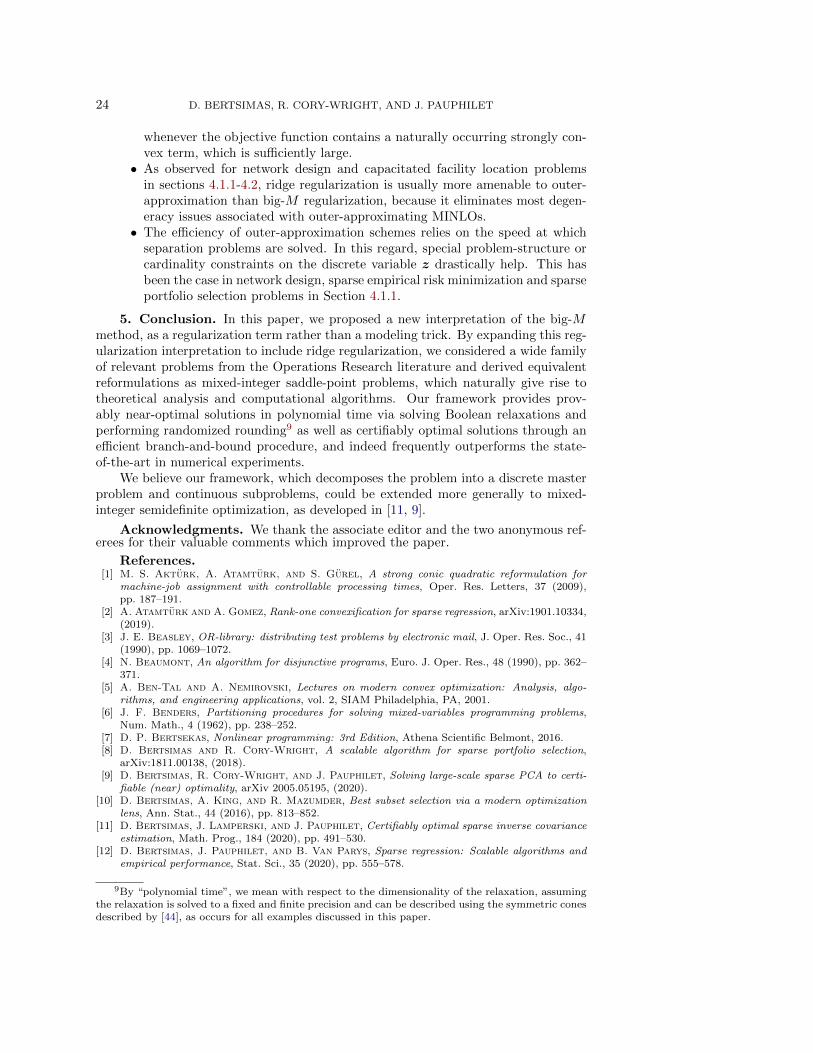
24 D. BERTSIMAS, R. CORY-WRIGHT, AND J. PAUPHILET
whenever the objective function contains a naturally occurring strongly con-vex term, which is sufficiently large.
• As observed for network design and capacitated facility location problemsin sections 4.1.1-4.2, ridge regularization is usually more amenable to outer-approximation than big-M regularization, because it eliminates most degen-eracy issues associated with outer-approximating MINLOs.
• The efficiency of outer-approximation schemes relies on the speed at whichseparation problems are solved. In this regard, special problem-structure orcardinality constraints on the discrete variable z drastically help. This hasbeen the case in network design, sparse empirical risk minimization and sparseportfolio selection problems in Section 4.1.1.
5. Conclusion. In this paper, we proposed a new interpretation of the big-Mmethod, as a regularization term rather than a modeling trick. By expanding this reg-ularization interpretation to include ridge regularization, we considered a wide familyof relevant problems from the Operations Research literature and derived equivalentreformulations as mixed-integer saddle-point problems, which naturally give rise totheoretical analysis and computational algorithms. Our framework provides prov-ably near-optimal solutions in polynomial time via solving Boolean relaxations andperforming randomized rounding9 as well as certifiably optimal solutions through anefficient branch-and-bound procedure, and indeed frequently outperforms the state-of-the-art in numerical experiments.
We believe our framework, which decomposes the problem into a discrete masterproblem and continuous subproblems, could be extended more generally to mixed-integer semidefinite optimization, as developed in [11, 9].
Acknowledgments. We thank the associate editor and the two anonymous ref-erees for their valuable comments which improved the paper.
References.[1] M. S. Akturk, A. Atamturk, and S. Gurel, A strong conic quadratic reformulation for
machine-job assignment with controllable processing times, Oper. Res. Letters, 37 (2009),pp. 187–191.
[2] A. Atamturk and A. Gomez, Rank-one convexification for sparse regression, arXiv:1901.10334,(2019).
[3] J. E. Beasley, OR-library: distributing test problems by electronic mail, J. Oper. Res. Soc., 41(1990), pp. 1069–1072.
[4] N. Beaumont, An algorithm for disjunctive programs, Euro. J. Oper. Res., 48 (1990), pp. 362–371.
[5] A. Ben-Tal and A. Nemirovski, Lectures on modern convex optimization: Analysis, algo-rithms, and engineering applications, vol. 2, SIAM Philadelphia, PA, 2001.
[6] J. F. Benders, Partitioning procedures for solving mixed-variables programming problems,Num. Math., 4 (1962), pp. 238–252.
[7] D. P. Bertsekas, Nonlinear programming: 3rd Edition, Athena Scientific Belmont, 2016.[8] D. Bertsimas and R. Cory-Wright, A scalable algorithm for sparse portfolio selection,
arXiv:1811.00138, (2018).[9] D. Bertsimas, R. Cory-Wright, and J. Pauphilet, Solving large-scale sparse PCA to certi-
fiable (near) optimality, arXiv 2005.05195, (2020).[10] D. Bertsimas, A. King, and R. Mazumder, Best subset selection via a modern optimization
lens, Ann. Stat., 44 (2016), pp. 813–852.[11] D. Bertsimas, J. Lamperski, and J. Pauphilet, Certifiably optimal sparse inverse covariance
estimation, Math. Prog., 184 (2020), pp. 491–530.[12] D. Bertsimas, J. Pauphilet, and B. Van Parys, Sparse regression: Scalable algorithms and
empirical performance, Stat. Sci., 35 (2020), pp. 555–578.
9By “polynomial time”, we mean with respect to the dimensionality of the relaxation, assumingthe relaxation is solved to a fixed and finite precision and can be described using the symmetric conesdescribed by [44], as occurs for all examples discussed in this paper.

A UNIFIED APPROACH TO MIXED-INTEGER OPTIMIZATION 25
[13] D. Bertsimas and B. Van Parys, Sparse high-dimensional regression: Exact scalable algo-rithms and phase transitions, Ann. Stat., 48 (2020), pp. 300–323.
[14] D. Bienstock, Computational study of a family of mixed-integer quadratic programming prob-lems, Math. Prog., 74 (1996), pp. 121–140.
[15] A. Billionnet and S. Elloumi, Using a mixed integer quadratic programming solver for theunconstrained quadratic 0-1 problem, Math. Prog., 109 (2007), pp. 55–68.
[16] P. Bonami and M. A. Lejeune, An exact solution approach for portfolio optimization problemsunder stochastic and integer constraints, Oper. Res., 57 (2009), pp. 650–670.
[17] S. Boyd and L. Vandenberghe, Convex optimization, Cambridge University Press, Cambridge,UK, 2004.
[18] X. Cui, X. Zheng, S. Zhu, and X. Sun, Convex relaxations and MIQCQP reformulationsfor a class of cardinality-constrained portfolio selection problems, J. Glob. Opt., 56 (2013),pp. 1409–1423.
[19] M. M. Deza and M. Laurent, Geometry of cuts and metrics, vol. 15, Springer, 2009.[20] H. Dong, K. Chen, and J. Linderoth, Regularization vs. relaxation: A conic optimization
perspective of statistical variable selection, arXiv:1510.06083, (2015).[21] I. Dunning, J. Huchette, and M. Lubin, JuMP: A modeling language for mathematical op-
timization, SIAM Rev., 59 (2017), pp. 295–320.[22] M. A. Duran and I. E. Grossmann, An outer-approximation algorithm for a class of mixed-
integer nonlinear programs, Math. Prog., 36 (1986), pp. 307–339.[23] M. Fischetti, I. Ljubic, and M. Sinnl, Benders decomposition without separability: A com-
putational study for capacitated facility location problems, Euro. J. Oper. Res., 253 (2016),pp. 557–569.
[24] M. Fischetti, I. Ljubic, and M. Sinnl, Redesigning Benders decomposition for large-scalefacility location, Mang. Sci., 63 (2016), pp. 2146–2162.
[25] R. Fletcher and S. Leyffer, Solving mixed integer nonlinear programs by outer approxima-tion, Math. Prog., 66 (1994), pp. 327–349.
[26] R. Fortet, Applications de l’algebre de boole en recherche operationelle, Revue Francaise deRecherche Operationelle, 4 (1960), pp. 17–26.
[27] A. Frangioni, F. Furini, and C. Gentile, Approximated perspective relaxations: a projectand lift approach, Comp. Opt. Appl., 63 (2016), pp. 705–735.
[28] A. Frangioni and C. Gentile, Perspective cuts for a class of convex 0–1 mixed integer pro-grams, Math. Prog., 106 (2006), pp. 225–236.
[29] A. Frangioni and C. Gentile, Solving nonlinear single-unit commitment problems with ramp-ing constraints, Oper. Res., 54 (2006), pp. 767–775.
[30] A. Frangioni and C. Gentile, SDP diagonalizations and perspective cuts for a class of non-separable MIQP, Oper. Res. Letters, 35 (2007), pp. 181–185.
[31] A. Frangioni and C. Gentile, A computational comparison of reformulations of the perspec-tive relaxation: Socp vs. cutting planes, Oper. Res. Letters, 37 (2009), pp. 206–210.
[32] J. Gao and D. Li, Optimal cardinality constrained portfolio selection, Oper. Res., 61 (2013),pp. 745–761.
[33] A. M. Geoffrion, Generalized Benders decomposition, J. Opt. Theory Appl., 10 (1972),pp. 237–260.
[34] F. Glover, Improved linear integer programming formulations of nonlinear integer problems,Mang. Sci., 22 (1975), pp. 455–460.
[35] M. X. Goemans and D. P. Williamson, Improved approximation algorithms for maximum cutand satisfiability problems using semidefinite programming, J. ACM, 42 (1995), pp. 1115–1145.
[36] O. Gunluk and J. Linderoth, Perspective reformulations of mixed integer nonlinear programswith indicator variables, Math. Prog., 124 (2010), pp. 183–205.
[37] O. Gunluk and J. Linderoth, Perspective reformulation and applications, in Mixed IntegerNonlinear Programming, Springer, 2012, pp. 61–89.
[38] K. Holmberg and J. Hellstrand, Solving the uncapacitated network design problem by alagrangean heuristic and branch-and-bound, Oper. Res., 46 (1998), pp. 247–259.
[39] K. Holmberg, M. Ronnqvist, and D. Yuan, An exact algorithm for the capacitated facilitylocation problems with single sourcing, Euro. J. Oper. Res., 113 (1999), pp. 544–559.
[40] J. E. Kelley, Jr, The cutting-plane method for solving convex programs, J. Soc. Ind. Appl.Math., 8 (1960), pp. 703–712.
[41] J. B. Lasserre, An explicit exact SDP relaxation for nonlinear 0-1 programs, in InternationalConference on Integer Programming and Combinatorial Optimization, Springer, 2001, pp. 293–303.
[42] M. Laurent, A comparison of the Sherali-Adams, Lovasz-Schrijver, and Lasserre relaxationsfor 0–1 programming, Math. Oper. Res., 28 (2003), pp. 470–496.

26 D. BERTSIMAS, R. CORY-WRIGHT, AND J. PAUPHILET
[43] T. L. Magnanti and R. T. Wong, Accelerating Benders decomposition: Algorithmic enhance-ment and model selection criteria, Oper. Res., 29 (1981), pp. 464–484.
[44] Y. Nesterov and A. Nemirovskii, Interior-point polynomial algorithms in convex program-ming, SIAM, 1994.
[45] M. Padberg and G. Rinaldi, A branch-and-cut algorithm for the resolution of large-scalesymmetric traveling salesman problems, SIAM Rev., 33 (1991), pp. 60–100.
[46] N. Papadakos, Practical enhancements to the Magnanti–Wong method, Oper. Res. Letters, 36(2008), pp. 444–449.
[47] M. Pilanci, M. J. Wainwright, and L. El Ghaoui, Sparse learning via Boolean relaxations,Math. Prog., 151 (2015), pp. 63–87.
[48] I. Quesada and I. E. Grossmann, An LP/NLP based branch and bound algorithm for convexMINLP optimization problems, Comp. & Chem. Eng., 16 (1992), pp. 937–947.
[49] P. Raghavan and C. D. Tompson, Randomized rounding: a technique for provably good algo-rithms and algorithmic proofs, Combinatorica, 7 (1987), pp. 365–374.
[50] J. Renegar and B. Grimmer, A simple nearly-optimal restart scheme for speeding-up firstorder methods, arXiv:1803.00151, (2018).
[51] P. Rigollet and J.-C. Hutter, High dimensional statistics, Lecture notes for course 18S997,(2015).
[52] J. P. Vielma, Mixed integer linear programming formulation techniques, SIAM Rev., 57 (2015),pp. 3–57.
[53] A. Wiegele, Biq Mac library—a collection of Max-Cut and quadratic 0-1 programming in-stances of medium size, tech. report, Alpen-Adria-Universitat Klagenfurt, Austria, 2007.
[54] W. Xie and X. Deng, Scalable algorithms for the sparse ridge regression, SIAM J. Opt., 30(2020), pp. 3359–3386.
[55] X. Zheng, X. Sun, and D. Li, Improving the performance of MIQP solvers for quadratic pro-grams with cardinality and minimum threshold constraints: A semidefinite program approach,INFORMS J. Comp., 26 (2014), pp. 690–703.
Appendix A. Omitted Proofs.
A.1. Proof of Theorem 3.1: Quality of the Random Rounding Strategy.
Proof. We only detail the proof for the big-M regularization case, as the ridgeregularization case follows mutatis mutandis. From Proposition 2.9,
0 ≤ f(z)− f(z?) ≤ML|R| maxα≥0:‖α‖1≤1
∑i∈R
(z?i − zi)αi.
The polyhedron α : α ≥ 0, ‖α‖1 ≤ 1 admits |R|+ 1 extreme points. However, if
maxα≥0:‖α‖1≤1
∑i∈R
(z?i − zi)αi > t,
for some t > 0, then the maximum can only occur at some α > 0 so that we canrestrict our attention to the |R| positive extreme points. Applying tail bounds on themaximum of sub-Gaussian random variables over a polytope [see 51, Theorem 1.16],since ‖α‖2 ≤ ‖α‖1 ≤ 1, we have for any t > 0,
P
(max
α≥0:‖α‖1≤1
∑i∈R
(z?i − zi)αi > t
)≤ |R| exp
(− t
2
2
),
so that
P
(ML|R| max
α≥0:‖α‖1≤1
∑i∈R
(z?i − zi)αi > ε
)≤ |R| exp
(− ε2
2M2L2|R|2
).

A UNIFIED APPROACH TO MIXED-INTEGER OPTIMIZATION 27
A.2. Proof of Theorem 3.2: Relationship With Perspective Cuts.
Proof. Let us fix z ∈ Z. Then, we have that:
maxα
h(α)− γ
2
n∑j=1
zjα2j = max
α,βh(α)− γ
2
n∑j=1
zj β2j s.t. β = α,
= maxα,β
minx
h(α)− γ
2
n∑j=1
zj β2j − x>(β −α),
= minx
maxα
[h(α) + x>α
]︸ ︷︷ ︸
(−h)?(x)=g(x)
+
n∑i=1
maxβi
[−γ
2zi β
2i − xiβi
].
Finally, observing that
maxβi
[−γ
2zi β
2i − xiβi
]=
x2i
2γziif zi > 0,
maxβi
xiβi if zj = 0,
concludes the proof.
Appendix B. Bounding the Lipschitz Constant. In our results, we reliedon the observation that there exists some constant L > 0 such that, for any z ∈ Z,‖α?(z)‖ ≤ L. Such an L always exists, since Z is a finite set. However, as ourrandomized rounding results depend on L, explicit bounds on L are desirable.
We remark that while our interest is in the Lipschitz constant with respect to“α” in a generic setting, we have used different notation for some of the problemswhich fit in our framework, in order to remain consistent with the literature. In thissense, we are also interested in obtaining a Lipschitz constant with respect to w forthe portfolio selection problem (2.5), among others.
In this appendix, we bound the magnitude of L in a less conservative manner. Ourfirst result provides a bound on L which holds whenever the function h(α) in Equation(2.14) is strongly concave in α, which occurs for the sparse ERM problem (2.4) withordinary least-squares loss, the unit commitment problem (2.7), the portfolio selection(2.5), and network design problems whenever Σ (resp. Q) is full-rank:
Lemma B.1. Let h(·) be a strongly concave function with parameter µ > 0 [see 17,Chapter 9.1.2 for a general theory of strong convexity], and suppose that 0 ∈ dom(g)and α? := arg maxα h(α). Then, for any choice of z, we have
‖α?(z)‖22 ≤ 8h(α?)− h(0)
µ,
i.e., ‖α?(z)‖∞ ≤ L, where L := 2√
2h(α?)−h(0)µ .
Proof. By the definition of strong concavity, for any α we have
h(α) ≤ h(α?) +∇h(α?)>(α−α?)− µ
2‖α−α?‖22,
where ∇h(α?)>(α − α?) ≤ 0 by the first-order necessary conditions for optimality,leading to
‖α−α?‖22 ≤ 2h(α?)− h(α)
µ.
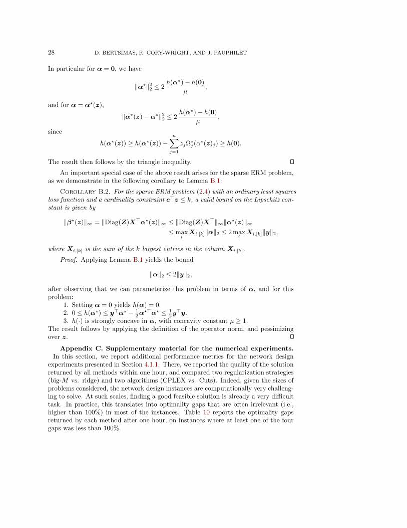
28 D. BERTSIMAS, R. CORY-WRIGHT, AND J. PAUPHILET
In particular for α = 0, we have
‖α?‖22 ≤ 2h(α?)− h(0)
µ,
and for α = α?(z),
‖α?(z)−α?‖22 ≤ 2h(α?)− h(0)
µ,
since
h(α?(z)) ≥ h(α?(z))−n∑j=1
zjΩ?j (α
?(z)j) ≥ h(0).
The result then follows by the triangle inequality.
An important special case of the above result arises for the sparse ERM problem,as we demonstrate in the following corollary to Lemma B.1:
Corollary B.2. For the sparse ERM problem (2.4) with an ordinary least squaresloss function and a cardinality constraint e>z ≤ k, a valid bound on the Lipschitz con-stant is given by
‖β?(z)‖∞ = ‖Diag(Z)X>α?(z)‖∞ ≤ ‖Diag(Z)X>‖∞‖α?(z)‖∞≤ max
iXi,[k]‖α‖2 ≤ 2 max
iXi,[k]‖y‖2,
where Xi,[k] is the sum of the k largest entries in the column Xi,[k].
Proof. Applying Lemma B.1 yields the bound
‖α‖2 ≤ 2‖y‖2,
after observing that we can parameterize this problem in terms of α, and for thisproblem:
1. Setting α = 0 yields h(α) = 0.2. 0 ≤ h(α?) ≤ y>α? − 1
2α?>α? ≤ 1
2y>y.
3. h(·) is strongly concave in α, with concavity constant µ ≥ 1.The result follows by applying the definition of the operator norm, and pessimizingover z.
Appendix C. Supplementary material for the numerical experiments.In this section, we report additional performance metrics for the network design
experiments presented in Section 4.1.1. There, we reported the quality of the solutionreturned by all methods within one hour, and compared two regularization strategies(big-M vs. ridge) and two algorithms (CPLEX vs. Cuts). Indeed, given the sizes ofproblems considered, the network design instances are computationally very challeng-ing to solve. At such scales, finding a good feasible solution is already a very difficulttask. In practice, this translates into optimality gaps that are often irrelevant (i.e.,higher than 100%) in most of the instances. Table 10 reports the optimality gapsreturned by each method after one hour, on instances where at least one of the fourgaps was less than 100%.
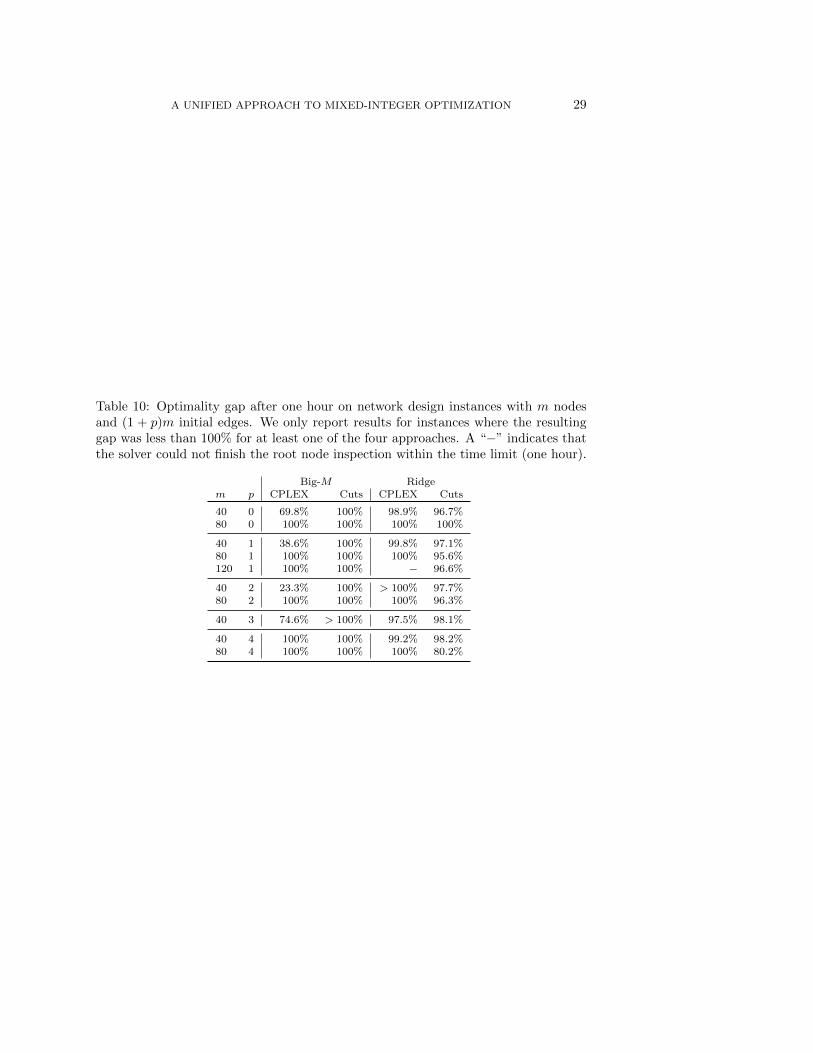
A UNIFIED APPROACH TO MIXED-INTEGER OPTIMIZATION 29
Table 10: Optimality gap after one hour on network design instances with m nodesand (1 + p)m initial edges. We only report results for instances where the resultinggap was less than 100% for at least one of the four approaches. A “−” indicates thatthe solver could not finish the root node inspection within the time limit (one hour).
Big-M Ridgem p CPLEX Cuts CPLEX Cuts
40 0 69.8% 100% 98.9% 96.7%80 0 100% 100% 100% 100%
40 1 38.6% 100% 99.8% 97.1%80 1 100% 100% 100% 95.6%120 1 100% 100% − 96.6%
40 2 23.3% 100% > 100% 97.7%80 2 100% 100% 100% 96.3%
40 3 74.6% > 100% 97.5% 98.1%
40 4 100% 100% 99.2% 98.2%80 4 100% 100% 100% 80.2%