A Two-Country Dynamic Stochastic Disequilibrium Model for ... · A Two-Country Dynamic Stochastic Disequilibrium Model for a Currency Union. Oliver Piceky Christian Schoderz April

A Two-Country Dynamic Stochastic Disequilibrium Model for a

Currency Union.∗

Oliver Picek† Christian Schoder‡

April 4, 2017

Abstract

The Dynamic Stochastic Dis-Equilibrium model introduced by Schoder (2017b) is extendedto a two-country version. Both countries are members of a monetary union. In the symmetricmodel calibration, effects of a domestic fiscal policy, a common monetary policy, a domesticproductivity shock, and a domestic wage bargaining shock are analyzed and impulse responsesprovided for both the domestic and foreign economy. In the asymmetric calibration, two distinctwage bargaining regimes (corporatist and conflictive) are attributed to the two countries. Thecorporatist economy generally fares better due to a superior external trade performance whenfaced with similar shocks. Finally, introducing a feedback from the trade balance to the wageformation process stabilizes the system.

Keywords: Dynamic stochastic disequilibrium, labor market disequilibrium, labor rationing,collective wage bargaining, monetary policyJEL Classification: B41, E12, J52

∗Financial support by the Hans-Bockler Foundation is gratefully acknowledged. The usual caveats apply.†Vienna University of Economics and Business, Welthandelsplatz 1, 1020 Vienna, Austria. Email:

[email protected]‡The New School for Social Research, 6 East 16th Street, New York, NY 10003. Email (corresponding author):

[email protected]

1

1 Introduction

During the first two decades of the European Monetary Union, internal current account imbalancesbetween Member States have seen a noticeable change in research interest. From it inception untilthe beginning of the Euro crisis, it was widely believed that current account imbalances betweenMember States have become irrelevant – comparable to current account differences between in-dividual states in a nation state with a common currency. Moreover, while the build-up of theimbalances was noticed, the overwhelming opinion was that they were “good” imbalances, coincid-ing at least to an extent to catching up-processes a la Balassa-Samuelson. With the onset of theEuro crisis came the uncertainty over a possible EMU break-up: In the absence of exchange rates tobet against, government bond yields slumped precisely in those Southern European countries (plusIreland) that had built up large external debt as a result of long-lasting current account deficits.Policymakers’ view towards internal imbalances began to shift despite the lender of last resort guar-antees by the European Central Bank. At the European Union level, an additional surveillancemechanism, the Macroeconomic Imbalances Procedure, was introduced by the European Commis-sion. Eventually, with massive austerity programs planned either by the TROIKA or fearful nationstates themselves, European policy embarked on an unprecedented adjustment effort and succeededwithin a couple years to bring down the current account deficits in Southern Europe.1 However,the corresponding surpluses of some Northern European countries, in particular Germany and theNetherlands, remained untouched. While their geographical origin shifted from Southern Europethat had compressed its import demand to countries outside of the monetary union, their level interms of GDP has increased even further.

Both of these experiences highlight the enormous persistence that current account imbalancesdisplay within the European Monetary Union, even for countries that are on a similar technologicallevel and share several industries. A number of channels have been identified that have contributedto the build-up of current account balances and, at least for the Northern countries, to their failureto revert back to the mean. The income channel ultimately refers to differences in relative growthrates. In DSGE models, the shock to government spending in the core has a high domestic multipliereffect if the economy is stuck in a liquidity trap and monetary policy is accomodative.2 The largerthe domestic shock, the larger will be the spillover effect to the foreign periphery economy viathe income channel. From the point of view of a domestic (Northern economy), if the foreign(Southern European) economy achieves higher growth rates for a number of years3, then a currentaccount surplus will arise simply because of the increasing cumulative difference in the relative sizeof final demand in the two economies.4 The second channel, the price and cost competitivenesschannel, is rooted in wage and inflation developments brought about by labor market forces and,as in our model, wage bargaining mechanisms. As Southern European economics expand and

1A similar development took place in the New Member States affected by simultaneous credit bubbles and currentaccount deficits.

2One of the key mechanisms for high multiplier effects is the real interest rate channel mentioned below.3under the assumption of ceteris paribus, including constant import propensities4In some countries, such as Spain and Ireland, the additional demand injection came about through a real estate

bubble in which increased private sector borrowing drove up real estate prices and spurred construction activity.In other countries, government spending was too high relative to the external constraint (Greece). As Picek andSchroder (2017) show in a multiregional input-output framework, direct demand spillover effects, however, have beensmall, even if one accounts for multiplier effects and global value chains. While basic IO models cannot capture pricecompetitiveness and monetary policy channels, they excel at simulating direct demand spillover effects through tradeat a level of regional detail that DSGE models cannot provide.

2

manage to lower their unemployment rates following an initial demand impulse, wage demands ofworkers increase, ultimately resulting in higher prices via a Phillips curve. With trade added tothe picture, the South loses relative cost and price competitiveness, and exports from the Northnow manage to capture an increasing market share in the South as long as demand traded costsis reasonably price-elastic. A large literature has debated cost competitiveness using unit laborcost developments among Euro Area countries, i.e. whether the the main causality goes fromdiverging wage levels (relative to labor productivity) to current account balances as claimed byLapavitsas and Flassbeck (2013). Most participants in the debate favor a weak role for cost andprice competitiveness as opposed to income effects (Gaulier and Vicard, 2012; Schroder, 2016;Storm and Naastepad, 2015; Gabrisch and Stahr, 2015). However, this part of the literature largelyforegoes any explicit macroeconomic modeling, which makes it hard to distinguish the effects ofthe different channels and keep track off all their spillover effects on the various markets. One suchchannel is the real interest rate channel that stimulates foreign demand indirectly if a domesticfiscal expansion increases the area-wide inflation rate as long as the central bank targets the area-wide rate. Lower foreign inflation then decreases the local real interest rate which makes optimizingagents switch consumption to the present in a standard Euler equation consumption framework. Inthe DSGE literature, these three channels can typically be found in two-country models of the sortthat we undertake in this paper. Among others, Blanchard et al. (2015) explicity attempt to modela core and periphery in the Euro Area, while Breuss and Rabitsch (2009), Andres et al. (2006)and Pytlarczyk (2005) focus on the Euro Area and one of its member states (Austria, Spain, andGermany, respectively). Finally, an effect that is unique to three- or multi-country models is theexchange rate channel.5 An expansion in the core lowers the exchange rate of the currency unionfrom which the periphery may profit as it raises price competitiveness and therefore net exportstowards third countries.

Wage dynamics play both an important causal and propagating role through several of thesechannels. Generally, a full macroeconomic model is preferable to disentangle the effect of severalof these shocks. However, particularly in regard to the DSGE models, the literature is rather smallbecause because wages are typically decentralized and privately efficient. Even worse, persistencein current account balances is hard to generate because of the general equilibrium structure of thesemodels. The main purpose of the present paper is to analyze in greater detail than comparableDSGE studies studies the role that divergent wage dynamics have played for persistent currentaccount imbalances. To this end, we extend the closed model framework of Schoder (2017a), whohas presented a Dynamic Stochastic Disequilibrium model, to a two-country model of a currencyunion. The original model combines disequilibrium theory with inter-temporal optimization andrational expectations. The fact that agents optimize makes it immune to the Lucas critique thatsimpler stock-flow consistent models of the Post-Keynesian tradition with aggregate parameters aresubject to. Likewise, in comparison to standard DSGE models, two particular advantages arise:Firstly, the rate of wage inflation is a policy variable subject to a collective bargaining processbetween firms’ and workers’ representatives rather than as an accommodating variable that givesrise to privately efficient wage contracts. Hence, the labor market does not clear in equilibrium andKeynesian unemployment prevails as labor is not employed optimally. Secondly, an uninsurable riskof permanent income loss is introduced to the household’s problem which motivates the existenceof precautionary savings and provides a mechanism by which consumption depends on income and

5Various extension and additional channels are possible. For instance, Poutineau and Vermandel (2015) includecross-border banking flows.

3

wealth even in equilibrium. Ultimately, this yields a Keynesian type of consumption function.With regard to the labor market, the model may be viewed as an attempt to understand policypropagation mechanisms if labor resources are permanently unter-utilized. While the model hasseveral policy implications, one of its strengths is that labor productivity and the real wage movetogether.

The model is calibrated to typical specifications in the literature. Firstly, we use an symmetriccalibration of the two economies to analyze separately an aysmmetric shock to wage bargaining,government spending, and total factor productivity as well as a common monetary policy shock.Impulse responses are provided for all of them for both the domestic and foreign economy. Acomparison with a standard DSGE model is drawn, highlighting the distinct Keynesian features ofthe model. The results of the closed economy version carry over to the currency union version. In asecond step, we calibrate the two economies symmetrically with the exception of one key difference.The domestic country runs on a corporatist wage formation regime, while the foreign country issubject to conflictive collective bargaining relations. A comparison of government spending shocksin the domestic and foreign economy as well as a common monetary policy shock reveals that thecorporatist regime generally fares better. This is largely due to their superior external performancewhen faced with these shocks. Finally, we analyze the introduction of feedback from the tradebalance to the wage formation process. In terms of recent policy discussions on current accountimbalances, this could be viewed as an adjustment in the goals of the domestic social partners in thecollective wage bargaining process to take into account the trade balance with the foreign country– and therefore policy in the monetary union to an extent. The introduction of this feedbackstabilizes the system by dampening the impulse response functions in both countries and in bothdirections, negative and positive.

The remainder of the paper is structured in a straighforward way. In Section 2, we presentthe model mainly along the lines of the domestic economy. In Section 3, we present the impulseresponse function for the major shocks and model versions. Finally, Section 4 concludes.

2 The model

The two-country model presented here is an extension of the Dynamic Stochastic Dis-Equilibriummodel introduced by Schoder (2017b). To keep the model tractable, we model the internationallinkages as in Pytlarczyk (2005) and Breuss and Rabitsch (2009). Both economies are populatedby active and inactive households, intermediate goods firms (producing heterogeneous consumptionand investment goods), final consumption and investment goods firms (bundling intermediate goodsin homogeneous final goods), retailers (combining domestic and foreign goods into consumption andinvestment aggregates), a fiscal policy authority, as well as workers’ and firms’ representatives inthe wage bargaining process. The monetary authority of the monetary union controls the commoninterest rate.

Details on the underlying DSDE model can be found in Schoder (2017b). The open economyaspects are further discussed in Pytlarczyk (2005) and Breuss and Rabitsch (2009). In this sectionwe restrain ourselves to stating the model equations and providing the intuition. Since we model theforeign country symmetric to the domestic country, we only present the equations for the domesticcountry. Note that an asterisk indicates a variable of the foreign country.

4

2.1 Households

As in Schoder (2017b), households are born in generations of constant size. Each newborn householdis part of the labor force–a state we refer to as active. Yet, the active household faces a constant per-period risk of becoming inactive losing all future labor and capital income. There is no insurancemarket for this risk. Once the household is inactive it cannot return to the active state. It facesthe risk of death with a constant probability. While active, the rational household will accumulateprecautionary savings as a buffer for the time when inactive.

We make three assumptions which allow us to derive closed-form relations of aggregated vari-ables despite partial wealth heterogeneity across households: First, inactive households have accessto a Blanchard (1985) insurance mechanism that ensures that there are no accidental bequests whendying. Bequests are transfered to inactive households that are still alive. Second, active householdsare subject to a transfer that enures that newborn households have the same wealth-income ratioas non-newborn active households. Third, we assume log-utility in consumption.

Under these assumptions, we can obtain the aggregated budget constraint of the inactive house-holds as

Ci,t + Bi,t =1

Γ

Rt−1

ΠC,t

(Bi,t−1 + UBa,t−1

)(1)

where the variables Ci,t, Bi,t, Rt, ΠC,t, and Bi,t denote consumption of the inactive households, end-of-period wealth of the inactive households, the gross interest rate, the inflation rate of consumerprices, and the wealth of active households, respectively. Γ is the determinstic growth rate of laborembodied productivity. Note that the tilde indicates variables that are detrended by deterministicgrowth. The budget constraint in equation (1) equates uses and sources of funds. The only non-standard feature is that sources include the previous period wealth of active households. This isbecause from period t − 1 to t a share of U of active households become inactive and bring theirwealth over.

The inactive household’s first order conditions (FOCs) imply that its period t consumption willbe proportional to its beginning-of-period wealth. Since the proportionality factor κ is constant wecan easily aggregate over all inactive households including newly inactive households to obtain

Ci,t = κ1

Γ

Rt−1

ΠC,t

(Bi,t−1 + UBa,t−1

)(2)

where κ = (1 − β(1 − D)) with β and D denoting the discount factor and the per-period risk ofdeath, respectively.

Equivalently, the active households budget constraints can be aggregated to yield

Ca,t + Ba,t = Zt + (1− U)1

Γ

Rt−1

ΠC,tBa,t−1 (3)

where Ca,t is consumption of active households and

Zt = ωtLt + Pt − pd,tTt (4)

is the active households’ real net income. ωt, Lt, Pt, pd,t, and Tt denote the real wage in termsof consumption goods, labor input, real profits in terms of consumption goods, prices of domestic

5

goods normalized by consumer prices, and real lump-sum taxes in terms of consumption goods.Note that Lt = (1− ut)Nt, which is implied by the definition of the unemployment rate

1− ut =LtNt, (5)

where Nt is labor supply and ut is the unemployment rate.The aggregated FOCs of the active households states that consumption should be chosen such

that the marginal utility in t is equal to the expected marginal utility in t+ 1. Since, the currentlyactive household may be newly inactive in the next period, the expected marginal utility alsodepends on the households consumption choice next period in case it became inactive. Hence, itinternalizes the optimal behavior of the inactive household. We get

θ

Ca,t= β(1− U)

1

ΓEt

RtΠC,t+1

θ

Ca,t+1

+ βU1

κBa,t(6)

where θ is a consumption utility scaling parameter. Note that this equation collapses to the standardEuler equation when U = 0.

Overall consumption is

Ct = Ca,t + Ci,t (7)

Aggregation of the FOC w.r.t. labor supply leads to

ψU1+ηNηt =

θ

Ca,tωt(1− ut). (8)

where ψ and η are a labor disutility scaling parameter and the inverse of the Frisch elasticity,respectively.

2.2 Firms

Retail firms. In the aggregate, households and firms purchase consumption bundles, Ct, andinvestment bundles, It, respectively. These bundles are generated by perfectly competitive repre-sentative consumption good retailers and investment good retailers, respectively. They combinehomogenous domestic final goods and foreign final goods using a Constant Elasticity of Substitution(CES) aggregator. The consumption retailers problem reads

maxCd,t,Cf,t

PC,tCt − (Pd,tCd,t + Pf,tCf,t)

s.t. Ct =(γc

1εcCd,t

εc−1εc + (1− γc)

1εcCf,t

εc−1εc

) εcεc−1

,

where Cd,t and Cf,t are the domestic and foreign final consumption good inputs, respectively, Pd,tand Pf,t are the prices of these goods, PC,t is the price of the final consumption bundle, γc is theshare of domestic consumption good inputs when domestic and foreign input prices are equal, andεc > 1 is the elasticity of substitution. Note that the government purchases domestic consumptiongoods straight from the final consumption goods firm and not from the retailer. The FOCs are

Cd,t = γcpd,t−εcCt (9)

6

and

Cf,t = (1− γc)pf,t−εcCt. (10)

With the optimal choice of Cd,t and Cf,t at a given Pd,t and Pf,t, one can compute the impliedaggregate price index of the consumption bundle as

1 =(γcpd,t

1−εc + (1− γc)pf,t1−εc) 1

1−εc (11)

The investment retailers problem is symmetric to the consumer retailers problem and yields theFOCs,

Id,t = γi

(pd,tpI,t

)−εiIt (12)

and

If,t = (1− γi)(pf,tpI,t

)−εiIt. (13)

With the optimal choice of Id,t and If,t at a given Pd,t and Pf,t, one can compute the impliedaggregate price index of the consumption bundle as

pI,t =(γipd,t

1−εi + (1− γi)pf,t1−εi) 1

1−εi . (14)

Final good firms. There are two symmetric representative perfectly competitive final goodsfirms: one for consumption goods and one for investment goods. The final goods firms purchaseonly domestic differentiated intermediate goods and bundle them into a homogeneous domesticconsumption good and a homogenous domestic investment good, respectively, sold to foreign anddomestic retailers. Taking as given price pi,t, the final consumption good firm’s demand for theintermediate good yC,i,t supplied by intermediate good firm i can be obtained from the followingcost minimization problem:

maxyC,i,t

Pd,t(Cd,t + C∗d,t +Gt +Ak,t +Ap,t)−∫ 1

0pi,tyC,i,tdi

s.t. Cd,t + C∗d,t +Gt +Ak,t +Ap,t =

∫ 1

0

(yC,i,t

ε−1ε di

) εε−1

,

where Gt is government spending, Ak,t and Ap,t are capital and price adjustment costs, respectively,and ε > 1 is the elasticity of substitution. Note that the asterisk denotes the foreign country. Notingthat the Lagrangian multiplier of the constraint is equal to the aggregate price index, PC,t, one canshow the FOC to read

yC,i,t =

(pi,tPd,t

)−ε(Cd,t + C∗d,t +Gd,t +Ak,t +Ap,t).

Equivalently, taking as given price pi,t, the final investment good firm’s demand for the intermediategood yI,i,t supplied by intermediate good firm i can be obtained as

yI,i,t =

(pi,tPd,t

)−ε(Id,t + I∗f,t).

7

Intermediate good firms. Taking as given total output Yt, the overall price level PC,t, and thewage rate ωt as well as the law of motion of capital, the production function, the demand functionfor intermediate goods, and the requirement to maintain a debt-capital ratio λ, the firm i chooses{pi,t, li,t, ii,t, ki,t, di,t}∞t=0 to maximize discounted inter-temporal distributed profits. Dropping thefirm index for convenience and evaluating at period t = 0, the optimization problem reads

max{pt,lt,it,kt,dt}∞t=0

E0

∞∑t=0

PC,0PC,t

Λ0,t

[ptyC,t + ptyI,t − PC,tωtlt − PI,tit − Pd,tAk,t − Pd,tAp,t+

+PC,tdt −Rt−1PC,t−1dt−1

]s.t. kt = it + (1− δ)kt−1

yC,t + yI,t = VA,t (Γkt−1)α (Γtlt)1−α

yC,t =

(ptPd,t

)−ε(Cd,t + C∗d,t +Gd,t +Ak,t +Ap,t)

yI,t =

(ptPd,t

)−ε(Id,t + I∗d,t)

Ak,t =τi2

(it

Γkt−1−(

1− (1− δ) 1

Γ

))2

kt−1

Ap,t =τp2

Γt(

ptPC,t−1

−Π

)2

dt = λqtkt

where ii,t, ki,t, di,t, VA,t, and qt are investment, the capital stock, outstanding bonds, total factorproductivity, and the price of capital, respectively. τi, δ, τp, and α denote the capital adjustmentcosts scaling parameter, the rate of capital depreciation, the price adjustment costs scaling parame-ter, and the capital elasticity of production. Λt,t+j is the stochastic discount factor which expressesthe value of a unit real profit in time t+ j in terms of the value of a unit real profit in time t.

The FOC w.r.t. dt implies that the financial structure of the firm is irrelevant from the house-hold’s perspective.

Regarding the price decision, note that all firms charge the same price, pt = Pd,t, independenton weather they are sold to the final consumption good or final investment good firm. HenceyC,t + yI,t = Yt with a mass one of firms. The FOC w.r.t. pt then implies(

(ε− 1)− ε ϕtpd,t

)Yt + τp (Πd,t −ΠC) Πd,t − EtΛt,t+1τpΓ (Πd,t+1 −ΠC)

Πd,t+12

ΠC,t+1= 0 (15)

where ϕt is the lagrangian multiplier of the production function constraint and has the interpreta-tion of real marginal costs and where

Λt−1,t =

(Rt−1

ΠC,t

)−1

(16)

as well as

Πd,t =pd,tpd,t−1

ΠC,t. (17)

8

The FOC w.r.t. lt, it, and kt imply

ϕt = ωt1

1− α

(1

VA,t

) 11−α

(Yt

Kt−1

) α1−α

, (18)

qt = pI,t + pd,tτi1

Γ

(It

Kt−1

−(

1− (1− δ) 1

Γ

)), (19)

and

qt = EtΛt,t+1

pd,t+1τi

(It+1

Kt−(1− (1− δ) 1

Γ

)) It+1

Kt−

−pd,t+1τi2

(It+1

Kt−(1− (1− δ) 1

Γ

))2+

+ϕt+1αYt+1

Kt+ qt+1(1− δ)

, (20)

respectively. Aggregating the law of motion of the capital stock leads to

Kt = It + (1− δ) 1

ΓKt−1 (21)

The aggregated production function reads

Yt = VA,tKαt−1L

1−αt . (22)

Recalling that firms maintain a debt-capital ratio of λ, the aggregated detrended real distributedprofits are

Πd,t = pd,tYt − ωtLt − (1− λ)pI,tIt − pd,tτi2

1

Γ

(It

Kt−1

−(

1− (1− δ) 1

Γ

))2

Kt−1−

− pd,tτp2

(ΠC,t −ΠC)2 . (23)

The growth rate of the real wage is linked to wage and price inflation according to

ωtωt−1

− 1 = Πw,t −ΠC,t. (24)

2.3 The labor market

We take the rate of wage inflation as subject to a bargaining process between a workers’ and afirms’ representative. We assume that the steady-state real wage ω(Πw,t) as the worker’s return andthe steady-state profit rate, r(Πw,t), as the firm’s return. Due to the presence of price adjustmentcosts, the former can be shown to increase and the latter to decrease in the rate of wage inflation.Hence, we suggest that the bargaining parties are concerned with the long-run implications of thebargaining. By assuming that the state of the labor market affects the relative bargaining power,however, the rate of wage inflation will be cyclical. The FOC of the bargaining game determinesthe rate of nominal wage inflation, Πw,t, and reads

1 = (1− 1/νt)ω(Πw,t)

r(Πw,t)

r′(Πw,t)

ω′(Πw,t). (25)

9

where

νtν

=

(1− ut1− u

)φuVν,t (26)

Note that there is not feedback of the labor market to wage formation if φu = 0. In this case, therate of wage inflation is constant.

2.4 Fiscal policy

We assume the government budget to be balanced at all times, i.e.

Tt = G (27)

Gt

G= VG,t (28)

2.5 Goods market clearing

As can easily be verified, aggregating over all budget constraints leads to the macro-economicbalance condition,

Yt = Cd,t + C∗d,t + Id,t + I∗d,t + G+

+τi2

1

Γ

(It

Kt−1

−(

1− (1− δ) 1

Γ

))2

Kt−1 +τp2

(ΠC,t −ΠC)2 (29)

2.6 Exogenous processes

The fiscal policy shock, monetary policy shock, total factor productivity shock, and worker bar-gaining power shock are assumed to evolve according to

VG,t = VG,t−1ρG exp εG,t, (30)

VR,t = VR,t−1ρR exp εR,t, (31)

VA,t = VA,t−1ρA exp εA,t, (32)

Vν,t = Vν,t−1ρν exp εν,t, (33)

where εG,t ∼ N (0, 1), εR,t ∼ N (0, 1), εA,t ∼ N (0, 1), and εν,t ∼ N (0, 1) are exogenous innovations.

10

2.7 International linkages

The final goods firms sell their products domestically and abroad. Under a common currency andwithout costs of trade,

Pd,t = P ∗d,t

Pf,t = P ∗f,t.

That is, a BMW sold in Germany needs to have the same price as a BMW sold in France. Equiva-lently, a Renault sold in Germany needs to have the same price as a Renault sold in France. Notehowever that pd,t 6= p∗d,t as PC,t 6= P ∗C,t. Defining the real exchange rate as Et = P ∗C,t/PC,t, we have

pd,t = p∗d,tEt (34)

pf,t = p∗f,tEt. (35)

Arbitrage between bonds implies a restriction on the real exchage rate (see Breuss and Rabitsch2008, footnote 8):

Et+1

Et=

Λ∗t,t+1/β∗

Λt,t+1/β. (36)

We assume the common monetary authority to set the interest rate according to

RtR

=

(ΠC,t

ΠC

)φrπVR,t (37)

3 Impulse response analysis

In the present section, we provide the impulse response analysis of four of the macroeconomic shocksin our baseline two-country DSDE model: A domestic productivity shock, a domestic fiscal policyshock, a common monetary policy shock, and, most importantly, a domestic wage bargaining shock.Whenever possible, we compare our disequilibrium version to a more standard DSGE version ofthe model to highlight the effects of the differences in the two model economies.

Moreover, we analyze modifications of the wage bargaining process in more detail. We may as-sume two distinct bargaining regimes for the two countries. Intuitively, unions and employers eitherwork together (corporatist) or fight each other (conflicting). Monetary and fiscal policies affect thetwo countries to a varying degree and in different ways when these particular regimes dominate thewage setting process. Finally, we ask what would happen if the wage bargaining process took intoaccount the current trade balance, i.e. the macroeconomic leeway (or restriction) that the externalconstraint provides serves as a feedback to the bargaining process. Regarding political relevance,the latter scenario particularly applies to calls for current account surplus countries within the EuroArea to inflate their economy.

In Figure 1, a shock to domestic total factor productivity of 1% of its steady state value isapplied. In a standard DSGE model (dashed line), higher labor productivity means an increase inthe marginal product of labor in the domestic economy. Without sticky wages, both the nominaland the real wage adjust instantaneously, so that full employment is guaranteed at all times. As themarginal product of labor has increased, the same output can be produced with less required labor

11

0 10 20 30 40

-0.1

0

0.1

0.2

0.3

0.4

%

0 10 20 30 40

-0.1

0

0.1

0.2

0.3

0.4

%

0 10 20 30 40-0.05

0

0.05

0.1

0.15

0.2

%

0 10 20 30 40-0.05

0

0.05

0.1

0.15

0.2

%

0 10 20 30 40

-0.05

0

0.05

0.1

0.15

%

0 10 20 30 40

-0.05

0

0.05

0.1

0.15

%

0 10 20 30 40

-0.3

-0.2

-0.1

0

pp

0 10 20 30 40

-0.3

-0.2

-0.1

0

pp

0 10 20 30 40

-1

-0.5

0

0.5

%

0 10 20 30 40

-1

-0.5

0

0.5

%

0 10 20 30 400

0.1

0.2

0.3

0.4

0.5

pp

0 10 20 30 400

0.1

0.2

0.3

0.4

0.5

pp

0 10 20 30 40-0.35

-0.3

-0.25

-0.2

-0.15

-0.1

-0.05

0

pp

0 10 20 30 400

0.05

0.1

0.15

0.2

0.25

0.3

0.35

%

0 10 20 30 400

0.1

0.2

0.3

0.4

%

0 10 20 30 400

0.010.020.030.040.050.060.070.08

%

Dom. output For. output Dom. consumption For. consumption

Dom. investment For. investment Dom. price inflation rate For. price inflation rate

Dom. real wage For. real wage Dom. unemployment rate For. unemployment rate

Interest rate Real exchange rate Terms of trade Trade balance

Figure 1: Macroeconomic responses to a productivity shock in the domestic country as predictedby the baseline DSDE model (solid line) and the corresponding DSGE model (dashed line).

input. Therefore, the domestic real wage falls by more than 1% initially to keep the equilibrium inthe labor market before converging back to the steady state value after a few periods. Indeed, itis here in the labor market that we see the biggest difference of the DSDE model to a comparableDSGE set-up. Instead of a fall in the real wage at full employment, domestic unemployment risesby more than .5 percentage points given the parameter calibrations. At the same time, the realwage increases slightly because wage inflation falls less than price inflation, lowering the mark-uptemporarily.Generally, however, a productivity shock is favorable in both the DSGE and the DSDE model forthe domestic economy as a whole. A higher marginal product of labor means that potential outputrises and a higher marginal product of capital means that firms demand more capital. Since capitaldoes not adjust instantaneously, investment is demanded and builds up the higher capital stockover the course of several periods. During this slow adjustment, multiplier effects are exerted and

12

lift up consumption and output. The effects are a bit weaker in the DSDE model than in the DSGEmodel because part of the potential additional output cannot be realized due to the increase in theunemployment rate.The foreign country suffers from the domestic productivity increase in the DSDE model. Sinceprices fall much more in the domestic economy than in the foreign one, the terms of trade worsenfor the foreign economy, and the real exchange rate increases. Consequently, the trade balance wors-ens as well form the point of view of the foreign economy. Output, consumption and investmentall fall. This is somewhat different in the DSGE model, where two countervailing forces interact.Therein, lower (domestic and foreign) prices pull up foreign real consumption, investment and out-put. However, the negative competitiveness effects dominate after period 1 through the terms oftrade. Foreign investment and output fall below the steady state level. In the DSDE model, the ad-ditional negative effect from the increase in unemployment shifts down the adjustment trajectoriesin output, investment and consumption.

In Figure 2, a 1% shock to domestic fiscal policy is simulated. While we assume a balancedbudget, the shock does have a positive multiplier effect on domestic output and unemployment fallscompared to its steady state level. As price inflation rises, the common central bank also raises thearea-wide interest rate. While this and other simultaneous effects do not manage to drive outputeffects to negative territory, they do so for investment and consumption. The terms of trade, thereal exchange rate and the trade balance all deteriorate from the point of view of the domesticcountry. The foreign economy of the DSDE model, however, sees an expansion that it would seeto such an extent in the DSGE model. Presumably, the stronger expansion rests on a combinationof the the wealth effect of an increase in the real interest rate and the employment effects of thespillovers from the domestic economy. Foreign output, investment and consumption all increase

In Figure 3, a common monetary policy shock of 1% (higher interest rates) meets the two(symmetrically calibrated) economies. Unsurprisingly, the effects are identical on both economies.This leaves the trade balance, the terms of trade and the real exchange rate constant (see the scale).The difference between the DSGE and the DSDE model is quite noteworty. Across the board, anegative wealth effect is present in the DSDE model. It lowers investment, consumption andoutput in both the domestic and foreign economy temporarily. While similar-looking short-termdynamics happen in the DSGE model for other reasons (intertemporal consumption smoothingthat makes households move their consumption from the present to the future), the wealth effect inthe disequilibrium model has permanent effects and brings about a new set of steady state valuesfor a few key variables. It occurs because the central bank feels obliged to keep the real interestrate at a permanently higher level due to a permanently higher price inflation rate. The latterarises due to a lower unemployment level in the new steady state that increases the bargainingpower of the union in the collective bargaining process. While output remains the same in the newsteady state, the shares of consumption and investment in output have shifted: Real consumptionis permanently elevated at over 0.2%, and investment permanently subdued at around -0.2% fromthe original steady state levels. Note the particular trajectory of the the unemployment rate: Afterthe initial increase in unemployment that is stark with almost three percentage points, a new steadystate is reached that features an almost 1% lower unemployment rate than in the original steadystate. Since the model is classical and not Keynesian in the model, this lower unemployment ratemust coincide with a new lower steady state value of the real wage (around -1%) when output hasconverged back to the old steady state.

In Figure 4, a 1% wage bargaining shock is applied to the domestic economy. Since collective

13

0 10 20 30 40

0

0.05

0.1

0.15%

0 10 20 30 40

0

0.05

0.1

0.15

%

0 10 20 30 40

-0.03

-0.02

-0.01

0

%

0 10 20 30 40

-0.03

-0.02

-0.01

0

%

0 10 20 30 40

-0.015

-0.01

-0.005

0

0.005

%

0 10 20 30 40

-0.015

-0.01

-0.005

0

0.005

%

0 10 20 30 400

0.01

0.02

0.03

0.04

0.05

pp

0 10 20 30 400

0.01

0.02

0.03

0.04

0.05

pp

0 10 20 30 40

0

0.1

0.2

0.3

%

0 10 20 30 40

0

0.1

0.2

0.3

%

0 10 20 30 40

-0.12

-0.1

-0.08

-0.06

-0.04

-0.02

0

pp

0 10 20 30 40

-0.12

-0.1

-0.08

-0.06

-0.04

-0.02

0

pp

0 10 20 30 400

0.01

0.02

0.03

0.04

0.05

pp

0 10 20 30 40-0.06

-0.05

-0.04

-0.03

-0.02

-0.01

0

%

0 10 20 30 40-0.06

-0.05

-0.04

-0.03

-0.02

-0.01

0

%

0 10 20 30 40-0.012

-0.01

-0.008

-0.006

-0.004

-0.002

0

%





Figure 2: Macroeconomic responses to a fiscal policy shock in the domestic country as predictedby the baseline DSDE model (solid line) and the corresponding DSGE model (dashed line).

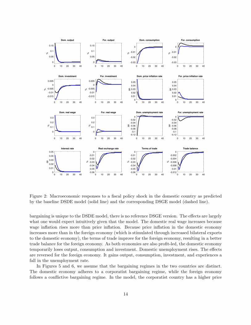
bargaining is unique to the DSDE model, there is no reference DSGE version. The effects are largelywhat one would expect intuitively given that the model. The domestic real wage increases becausewage inflation rises more than price inflation. Because price inflation in the domestic economyincreases more than in the foreign economy (which is stimulated through increased bilateral exportsto the domestic economy), the terms of trade improve for the foreign economy, resulting in a bettertrade balance for the foreign economy. As both economies are also profit-led, the domestic economytemporarily loses output, consumption and investment. Domestic unemployment rises. The effectsare reversed for the foreign economy. It gains output, consumption, investment, and experiences afall in the unemployment rate.

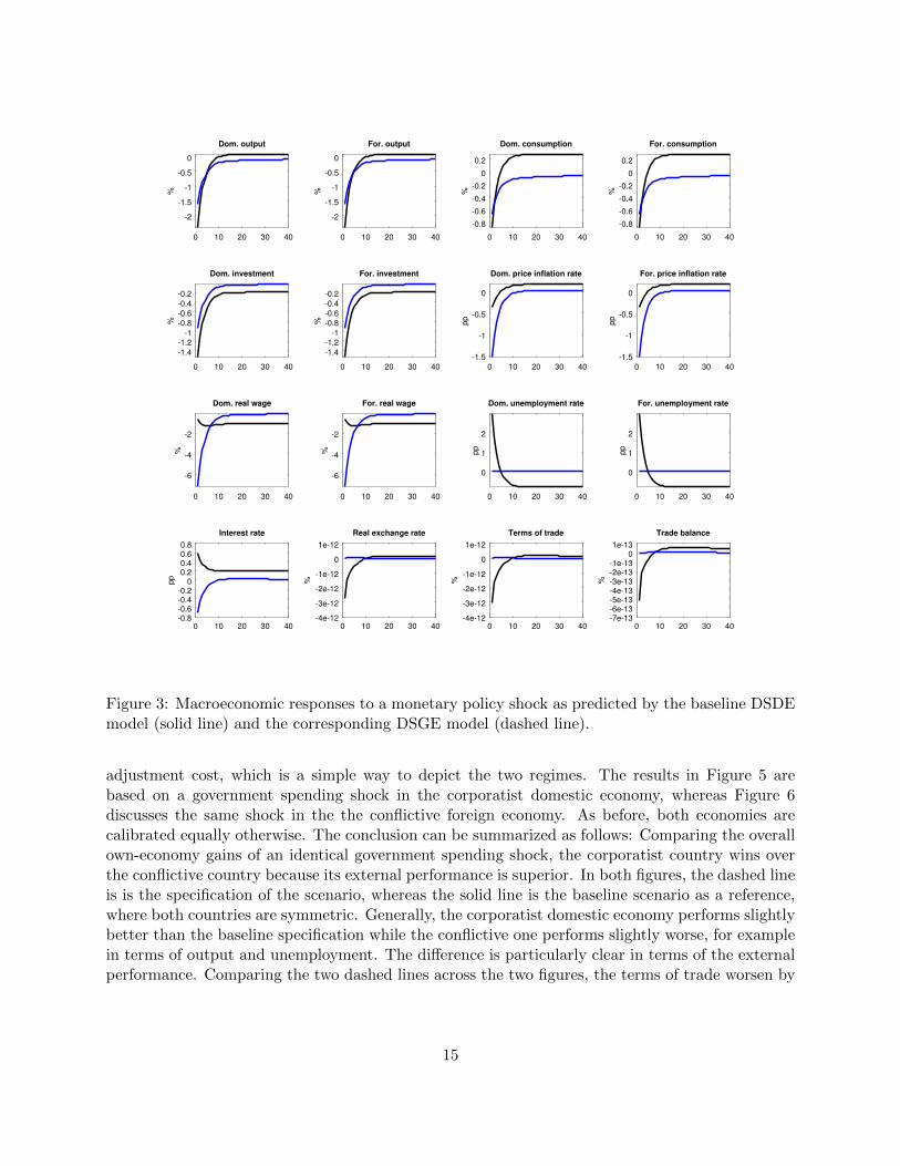
In Figures 5 and 6, we assume that the bargaining regimes in the two countries are distinct.The domestic economy adheres to a corporatist bargaining regime, while the foreign economyfollows a conflictive bargaining regime. In the model, the corporatist country has a higher price

14

0 10 20 30 40

-2

-1.5

-1

-0.5

0

%

0 10 20 30 40

-2

-1.5

-1

-0.5

0

%

0 10 20 30 40

-0.8

-0.6

-0.4

-0.2

0

0.2

%

0 10 20 30 40

-0.8

-0.6

-0.4

-0.2

0

0.2

%

0 10 20 30 40

-1.4

-1.2

-1

-0.8

-0.6

-0.4

-0.2

%

0 10 20 30 40

-1.4

-1.2

-1

-0.8

-0.6

-0.4

-0.2

%

0 10 20 30 40

-1.5

-1

-0.5

0

pp

0 10 20 30 40

-1.5

-1

-0.5

0

pp

0 10 20 30 40

-6

-4

-2

%

0 10 20 30 40

-6

-4

-2

%

0 10 20 30 40

0

1

2

pp

0 10 20 30 40

0

1

2

pp

0 10 20 30 40-0.8-0.6-0.4-0.2

00.20.40.60.8

pp

0 10 20 30 40-4e-12

-3e-12

-2e-12

-1e-12

0

1e-12

%

0 10 20 30 40-4e-12

-3e-12

-2e-12

-1e-12

0

1e-12

%

0 10 20 30 40-7e-13-6e-13-5e-13-4e-13-3e-13-2e-13-1e-13

01e-13

%





Figure 3: Macroeconomic responses to a monetary policy shock as predicted by the baseline DSDEmodel (solid line) and the corresponding DSGE model (dashed line).

adjustment cost, which is a simple way to depict the two regimes. The results in Figure 5 arebased on a government spending shock in the corporatist domestic economy, whereas Figure 6discusses the same shock in the the conflictive foreign economy. As before, both economies arecalibrated equally otherwise. The conclusion can be summarized as follows: Comparing the overallown-economy gains of an identical government spending shock, the corporatist country wins overthe conflictive country because its external performance is superior. In both figures, the dashed lineis is the specification of the scenario, whereas the solid line is the baseline scenario as a reference,where both countries are symmetric. Generally, the corporatist domestic economy performs slightlybetter than the baseline specification while the conflictive one performs slightly worse, for examplein terms of output and unemployment. The difference is particularly clear in terms of the externalperformance. Comparing the two dashed lines across the two figures, the terms of trade worsen by

15

0 10 20 30 40

-0.04

-0.02

0

0.02%

0 10 20 30 40

-0.04

-0.02

0

0.02

%

0 10 20 30 40

-0.02

-0.01

0

0.01

%

0 10 20 30 40

-0.02

-0.01

0

0.01

%

0 10 20 30 40

-0.02-0.015-0.01

-0.0050

0.0050.01

%

0 10 20 30 40

-0.02-0.015-0.01

-0.0050

0.0050.01

%

0 10 20 30 400

0.005

0.01

0.015

0.02

0.025

pp

0 10 20 30 400

0.005

0.01

0.015

0.02

0.025

pp

0 10 20 30 40

0

0.05

0.1

0.15

0.2

%

0 10 20 30 40

0

0.05

0.1

0.15

0.2

%

0 10 20 30 40-0.04-0.02

00.020.040.060.080.1

pp

0 10 20 30 40-0.04-0.02

00.020.040.060.080.1

pp

0 10 20 30 400

0.005

0.01

0.015

0.02

pp

0 10 20 30 40-0.08-0.07-0.06-0.05-0.04-0.03-0.02-0.01

%

0 10 20 30 40-0.08-0.07-0.06-0.05-0.04-0.03-0.02-0.01

%

0 10 20 30 40-0.0007-0.0006-0.0005-0.0004-0.0003-0.0002-0.0001

0

%





Figure 4: Macroeconomic responses to a wage bargaining power shock as predicted by the baselineDSDE model.

only .3% as a minimum in the corporatist regime, but by almost .6% in the conflictive regime.6 Asa result, the trade balance worsen by around .01% in the conflictive foreign country, but only byaround .5% in the corporatist domestic country. One noteworthy difference arises in the behaviorof the real wage. In the conflictive country, a government spending shock induces double themaximum rise in the foreign real wage as compared to the baseline model. If the shock hits thedomestic economy, however, the domestic real wage remains suppressed and actually falls.

In Figure 7, a common monetary policy of 1% shock affects the two countries differently whenthe domestic country is coporatist and the foreign country conflictive. Domestic output, investment,consumption and employment remain permanently above the baseline scenario, while their foreignequivalents remains below. The trade balance changes temporarily in favor of the domestic of thedomestic economy. The real wage in the two economies diverges in the long run, rising in the

6The trade balance is always depicted from the point of view of the domestic country.

16

0 10 20 30 40

0

0.05

0.1

0.15%

0 10 20 30 40

0

0.05

0.1

0.15

%

0 10 20 30 40

-0.015

-0.01

-0.005

0

0.005

%

0 10 20 30 40

-0.015

-0.01

-0.005

0

0.005

%

0 10 20 30 40

-0.01

-0.005

0

0.005

%

0 10 20 30 40

-0.01

-0.005

0

0.005

%

0 10 20 30 40

0

0.005

0.01

0.015

0.02

pp

0 10 20 30 40

0

0.005

0.01

0.015

0.02

pp

0 10 20 30 40

-0.02

-0.01

0

0.01

%

0 10 20 30 40

-0.02

-0.01

0

0.01

%

0 10 20 30 40-0.15

-0.1

-0.05

0

pp

0 10 20 30 40-0.15

-0.1

-0.05

0

pp

0 10 20 30 400

0.005

0.01

0.015

0.02

pp

0 10 20 30 40-0.04

-0.03

-0.02

-0.01

0

%

0 10 20 30 40-0.05

-0.04

-0.03

-0.02

-0.01

0

%

0 10 20 30 40-0.01

-0.008

-0.006

-0.004

-0.002

0

%





Figure 5: Macroeconomic responses to a government spending shock in the domestic country aspredicted by the baseline specification (solid line) and a conflictive foreign country/corporatistdomestic country specficition (dashed line).

domestic one and falling in the foreign one, while the price inflation rate converges back to thesame level after an initial opposing reaction. Compared to the fiscal policy shocks in the previoustwo figures, the foreign economy fares even worse when faced with a monetary policy shock.

In Figure 8, we introduce a feedback of the trade balance on wage bargaining power. The idea isthat enough political pressure is applied on the domestic country so that the collective bargainingwage formation process (presumably among social partners) begins to take into account the externalbalance in their decision-making. In case of a postive trade balance, the wage bargaining power ofunions will therefore be weaker, and in case of a negative trade balance, the power of employers willbe weaker. The figure compares the baseline model (solid) to the model with trade balance feedbackon the bargaining process (dashed) when a bargaining shock hits the domestic economy. Given theparameter calibration, the real exchange rate, terms of trade and the trade balance deviations are

17

0 10 20 30 40

0

0.05

0.1

0.15%

0 10 20 30 40

0

0.05

0.1

0.15

%

0 10 20 30 40

-0.015

-0.01

-0.005

0

0.005

0.01

%

0 10 20 30 40

-0.015

-0.01

-0.005

0

0.005

0.01

%

0 10 20 30 40

-0.01

-0.005

0

0.005

0.01

%

0 10 20 30 40

-0.01

-0.005

0

0.005

0.01

%

0 10 20 30 40

0

0.005

0.01

0.015

0.02

pp

0 10 20 30 40

0

0.005

0.01

0.015

0.02

pp

0 10 20 30 40

-0.02

0

0.02

0.04

%

0 10 20 30 40

-0.02

0

0.02

0.04

%

0 10 20 30 40

-0.12

-0.1

-0.08

-0.06

-0.04

-0.02

0

pp

0 10 20 30 40

-0.12

-0.1

-0.08

-0.06

-0.04

-0.02

0

pp

0 10 20 30 40-0.005

0

0.005

0.01

0.015

0.02

pp

0 10 20 30 400

0.01

0.02

0.03

0.04

0.05

0.06

%

0 10 20 30 400

0.01

0.02

0.03

0.04

0.05

0.06

%

0 10 20 30 400

0.002

0.004

0.006

0.008

0.01

0.012

%





Figure 6: Macroeconomic responses to a government spending shock in the foreign country aspredicted by the baseline specification (solid line) and a conflictive foreign country/corporatistdomestic country specficition (dashed line).

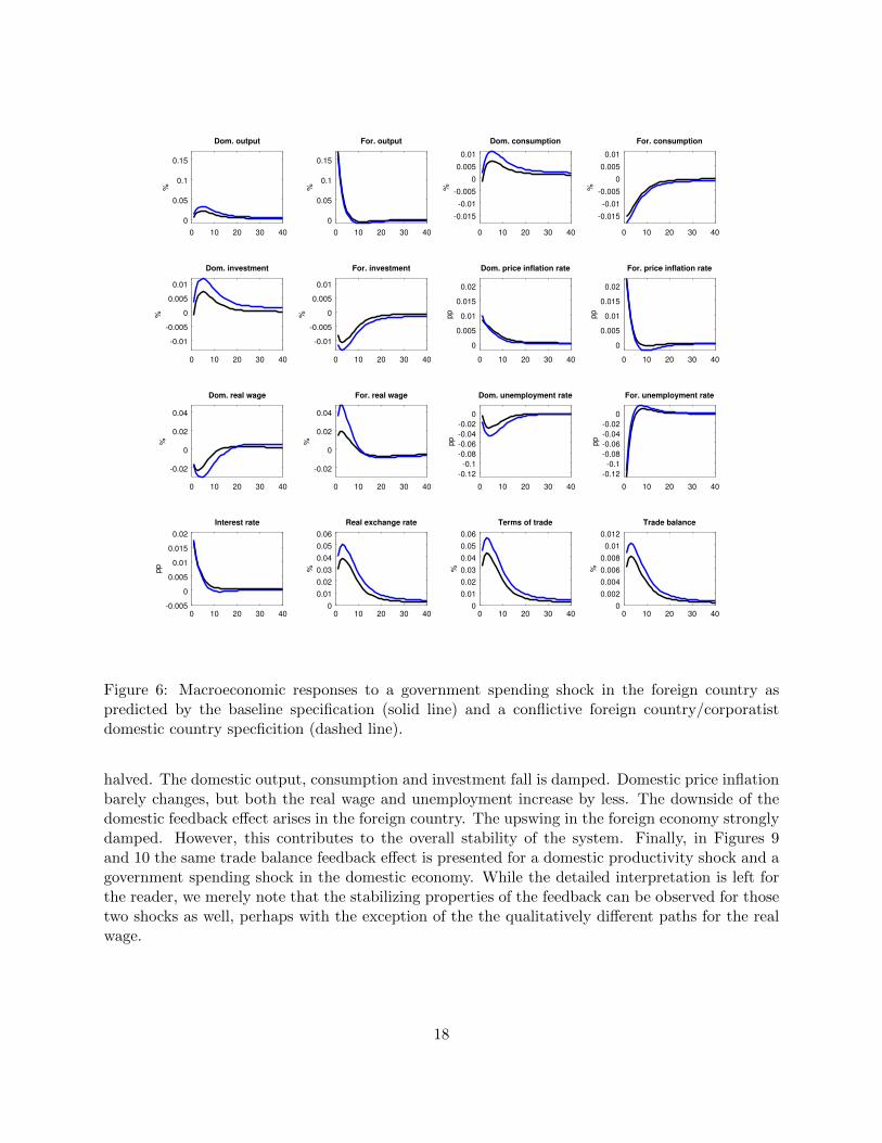
halved. The domestic output, consumption and investment fall is damped. Domestic price inflationbarely changes, but both the real wage and unemployment increase by less. The downside of thedomestic feedback effect arises in the foreign country. The upswing in the foreign economy stronglydamped. However, this contributes to the overall stability of the system. Finally, in Figures 9and 10 the same trade balance feedback effect is presented for a domestic productivity shock and agovernment spending shock in the domestic economy. While the detailed interpretation is left forthe reader, we merely note that the stabilizing properties of the feedback can be observed for thosetwo shocks as well, perhaps with the exception of the the qualitatively different paths for the realwage.

18

0 10 20 30 40

-4

-2

0%

0 10 20 30 40

-4

-2

0

%

0 10 20 30 40

-1.5

-1

-0.5

0

0.5

%

0 10 20 30 40

-1.5

-1

-0.5

0

0.5

%

0 10 20 30 40-3

-2

-1

0

%

0 10 20 30 40-3

-2

-1

0

%

0 10 20 30 40-1.5

-1

-0.5

0

0.5

pp

0 10 20 30 40-1.5

-1

-0.5

0

0.5

pp

0 10 20 30 40-3

-2.5

-2

-1.5

-1

-0.5

%

0 10 20 30 40-3

-2.5

-2

-1.5

-1

-0.5

%

0 10 20 30 40-2

0

2

4

6

pp

0 10 20 30 40-2

0

2

4

6

pp0 10 20 30 40

0.1

0.2

0.3

0.4

0.5

0.6

0.7

pp

0 10 20 30 40-1

0

1

2

3

4

5

%

0 10 20 30 40-1

0

1

2

3

4

5

%

0 10 20 30 40-0.2

0

0.2

0.4

0.6

0.8

%





Figure 7: Macroeconomic responses to a monetary policy shock as predicted by the baseline speci-fication (solid line) and a conflictive foreign country/coroporationist domestic country specficition(dashed line).

4 Conclusion

In the present paper, we have extended the closed economy model of Schoder (2017b) to a two-country version of a currency union with a particular focus on wage bargaining. Four main con-clusions emerge. Firstly, we have provided a model that is at the same time capable of analyzingthe wage bargainging process while a being micro-founded and thus grounded in intertemporal op-timization. Standard DSGE models deliver predictions for the wage bargaining process that are atodds with empirical evidence. By modeling the wage formation process as a collective bargaininggame, we manage to introduce unemployment into the model that affects bargaining power whichin turn affects the real wage. By extending the model to two countries, we can analyze spillovereffects of shocks to wages in one economy. Secondly, trade imbalances are slightly more persistentin DSDE models than in DSGE models. Thirdly, when recommendations for policy are form-

19

0 10 20 30 40

-0.04

-0.02

0

0.02%

0 10 20 30 40

-0.04

-0.02

0

0.02

%

0 10 20 30 40

-0.02

-0.015

-0.01

-0.005

0

0.005

0.01

%

0 10 20 30 40

-0.02

-0.015

-0.01

-0.005

0

0.005

0.01

%

0 10 20 30 40

-0.02

-0.015

-0.01

-0.005

0

0.005

0.01

%

0 10 20 30 40

-0.02

-0.015

-0.01

-0.005

0

0.005

0.01

%

0 10 20 30 400

0.005

0.01

0.015

0.02

pp

0 10 20 30 400

0.005

0.01

0.015

0.02

pp

0 10 20 30 40

0

0.05

0.1

0.15

0.2

%

0 10 20 30 40

0

0.05

0.1

0.15

0.2

%

0 10 20 30 40-0.05

0

0.05

0.1

pp

0 10 20 30 40-0.05

0

0.05

0.1

pp

0 10 20 30 400

0.005

0.01

0.015

0.02

pp

0 10 20 30 40-0.08-0.07-0.06-0.05-0.04-0.03-0.02-0.01

0

%

0 10 20 30 40-0.08

-0.06

-0.04

-0.02

0

%

0 10 20 30 40-0.014

-0.012

-0.01

-0.008

-0.006

-0.004

-0.002

0

%





Figure 8: Macroeconomic responses to a wage bargaining power shock in the domestic country aspredicted by the baseline DSDE model (solid line) and a DSDE model with trade balance feedbackon the wage bargaining power (dashed line).

lated to eliminate current account imbalances, the wage setting regimes of the individual countriesneed to be understood and respected. A corporatist and a conflictive bargaining system underthe umbrella of a common monetary union will react differently when faced with symmetric andasymmetric shocks. The size of the policy shocks and the resulting policy mix should be adjustedaccordingly. Finally, taking current account imbalances into accout when in the formulation ofwage setting policy may be an advantage. The business cycle (when interpreted as the result ofvarious policy as well as a productivity shock) is decidely more stable when this feedback processis introduced to wage formation in our model because fluctuations are damped.

20

0 10 20 30 40

-0.1

0

0.1

0.2

%

0 10 20 30 40

-0.1

0

0.1

0.2

%

0 10 20 30 40

-0.05

0

0.05

0.1

%

0 10 20 30 40

-0.05

0

0.05

0.1

%

0 10 20 30 40

-0.05

0

0.05

0.1

%

0 10 20 30 40

-0.05

0

0.05

0.1

%

0 10 20 30 40

-0.15

-0.1

-0.05

0

pp

0 10 20 30 40

-0.15

-0.1

-0.05

0

pp

0 10 20 30 40-0.2

0

0.2

0.4

0.6

%

0 10 20 30 40-0.2

0

0.2

0.4

0.6

%

0 10 20 30 40

0

0.1

0.2

0.3

0.4

0.5

0.6

pp

0 10 20 30 40

0

0.1

0.2

0.3

0.4

0.5

0.6

pp

0 10 20 30 40-0.2

-0.15

-0.1

-0.05

0

pp

0 10 20 30 40-0.1

0

0.1

0.2

0.3

0.4

%

0 10 20 30 40-0.1

0

0.1

0.2

0.3

0.4

%

0 10 20 30 40-0.02

0

0.02

0.04

0.06

0.08

%





Figure 9: Macroeconomic responses to a productivity shock in the domestic country as predictedby the baseline DSDE model (solid line) and a DSDE model with trade balance feedback on thewage bargaining power (dashed line).

21

0 10 20 30 40

0

0.05

0.1

0.15

%

0 10 20 30 40

0

0.05

0.1

0.15

%

0 10 20 30 40

-0.015

-0.01

-0.005

0

0.005

%

0 10 20 30 40

-0.015

-0.01

-0.005

0

0.005

%

0 10 20 30 40

-0.01

-0.005

0

0.005

%

0 10 20 30 40

-0.01

-0.005

0

0.005

%

0 10 20 30 40

0

0.005

0.01

0.015

0.02

pp

0 10 20 30 40

0

0.005

0.01

0.015

0.02

pp

0 10 20 30 40

-0.02

-0.01

0

0.01

0.02

%

0 10 20 30 40

-0.02

-0.01

0

0.01

0.02

%

0 10 20 30 40

-0.14

-0.12

-0.1

-0.08

-0.06

-0.04

-0.02

0

pp

0 10 20 30 40

-0.14

-0.12

-0.1

-0.08

-0.06

-0.04

-0.02

0

pp

0 10 20 30 400

0.005

0.01

0.015

0.02

pp

0 10 20 30 40-0.04

-0.03

-0.02

-0.01

0

0.01

%

0 10 20 30 40-0.05

-0.04

-0.03

-0.02

-0.01

0

0.01

%

0 10 20 30 40-0.01

-0.008

-0.006

-0.004

-0.002

0

0.002

%





Figure 10: Macroeconomic responses to a government spending shock in the domestic country aspredicted by the baseline DSDE model (solid line) and a DSDE model with trade balance feedbackon the wage bargaining power (dashed line).

22

References

Andres, J., Burriel, P., and Estrada, A. (2006). Bemod: A dsge model for the spanish economyand the rest of the euro area.

Blanchard, O., Erceg, C. J., and Linde, J. (2015). Jump starting the euro area recovery: would arise in core fiscal spending help the periphery? Technical report, National Bureau of EconomicResearch.

Blanchard, O. J. (1985). Debt, deficits, and finite horizons. The Journal of Political Economy,93(2):pp. 223–247.

Breuss, F. and Rabitsch, K. (2009). An estimated two-country dsge model of austria and the euroarea. Empirica, 36(1):123–158.

Gabrisch, H. and Stahr, K. (2015). The euro plus pact: Competitiveness and external capital flowsin the eu countries. JCMS: Journal of Common Market Studies, 53(3):558–576.

Gaulier, G. and Vicard, V. (2012). Current account imbalances in the euro area: competitivenessor demand shock? Bank of France Quarterly Selection of Articles, (27).

Lapavitsas, C. and Flassbeck, H. (2013). The systemic crisis of the euro – true causes and effectivetherapies. Rosa-Luxemburg-Stiftung, Berlin, Germany. May 2013.

Picek, O. and Schroder, E. (2017). Spillover Effects of Germany’s Final Demand on SouthernEurope. New School Economics Department Working Paper Series (forthcoming).

Poutineau, J.-C. and Vermandel, G. (2015). Cross-border banking flows spillovers in the eurozone:Evidence from an estimated dsge model. Journal of Economic Dynamics and Control, 51:378–403.

Pytlarczyk, E. (2005). An estimated dsge model for the german economy within the euro area. Tech-nical report, Discussion paper Series 1/Volkswirtschaftliches Forschungszentrum der DeutschenBundesbank.

Schoder, C. (2017a). A keynesian dynamic stochastic disequilibrium model for business cycleanalysis. Technical report.

Schoder, C. (2017b). A keynesian dynamic stochastic labor market disequilibrium model for busi-ness cycle analysis. Working Paper 1, New School Working Paper Series, Dusseldorf, Germany.

Schroder, E. (2016). Euro area imbalances: Measuring the contribution of expenditure growth andexpenditure switching. New School Working Paper, WP(04). August.

Storm, S. and Naastepad, C. W. M. (2015). Europe’s hunger games: Income distribution, costcompetitiveness and crisis. Cambridge Journal of Economics, 39(3):959–986.

23

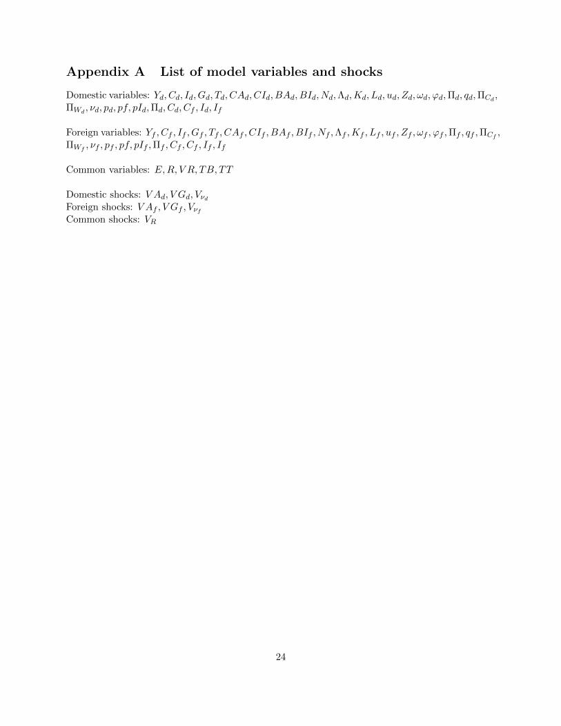
Appendix A List of model variables and shocks

Domestic variables: Yd, Cd, Id, Gd, Td, CAd, CId, BAd, BId, Nd,Λd,Kd, Ld, ud, Zd, ωd, ϕd,Πd, qd,ΠCd ,ΠWd

, νd, pd, pf, pId,Πd, Cd, Cf , Id, If

Foreign variables: Yf , Cf , If , Gf , Tf , CAf , CIf , BAf , BIf , Nf ,Λf ,Kf , Lf , uf , Zf , ωf , ϕf ,Πf , qf ,ΠCf ,ΠWf

, νf , pf , pf, pIf ,Πf , Cf , Cf , If , If

Common variables: E,R, V R, TB, TT

Domestic shocks: V Ad, V Gd, VνdForeign shocks: V Af , V Gf , VνfCommon shocks: VR

24

Appendix B Parameter calibration

Table 1: Parameter calibration

Common parameters:φrpi 1.1R 1.004ρR 0.7Domestic parameters:Γd 1.01βd 0.998Dd 0.002Ud 0.3 ∗Dd

κd 1− βd · (1−Dd)ηd 1δd 0.025εd 3εid 3εcd 3λd 0.15τid 20τpd 30φνud 2

φνtbd 20

ρGd 0.7ρνd 0.7ρAd 0.7Gd 0.2

¯PICd 1¯Y Kd 0.1Yd 1ud 0γcd 0.95γid 0.95Foreign parameters: equal to domestic ones (symmetric calibration)

25

Documents

A Two-Country Dynamic Stochastic Disequilibrium Model for ... · A Two-Country Dynamic Stochastic Disequilibrium Model for a Currency Union. Oliver Piceky Christian Schoderz April