A Tutorial for Spice3 / Nutmeg - Universidad de Sevillaiecon02.us.es/ASIGN/DCSE_1IE/WinSpice_tutorial.pdf · gate M1 2 1 0 0 modn a MOS gate over nodes 2 ... nor work exactly the

Spice3 Tutorial

A Tutorial for Spice3 / Nutmeg

Mike Smith

Based on a tutorial by Sanford Staab

Copyright 1999 Mike Smith 1

Spice3 Tutorial

This tutorial is intended to help the first-time SPICE3 user. One will learn how to properly create circuit description input files and how each of the different types of circuit analysis can be performed. NUTMEG is a powerful I/O driver program designed to make the analysis of circuits with SPICE3 more interactive and efficient. A mastery of these two tools will greatly help the reader to understand and design electronic circuits.

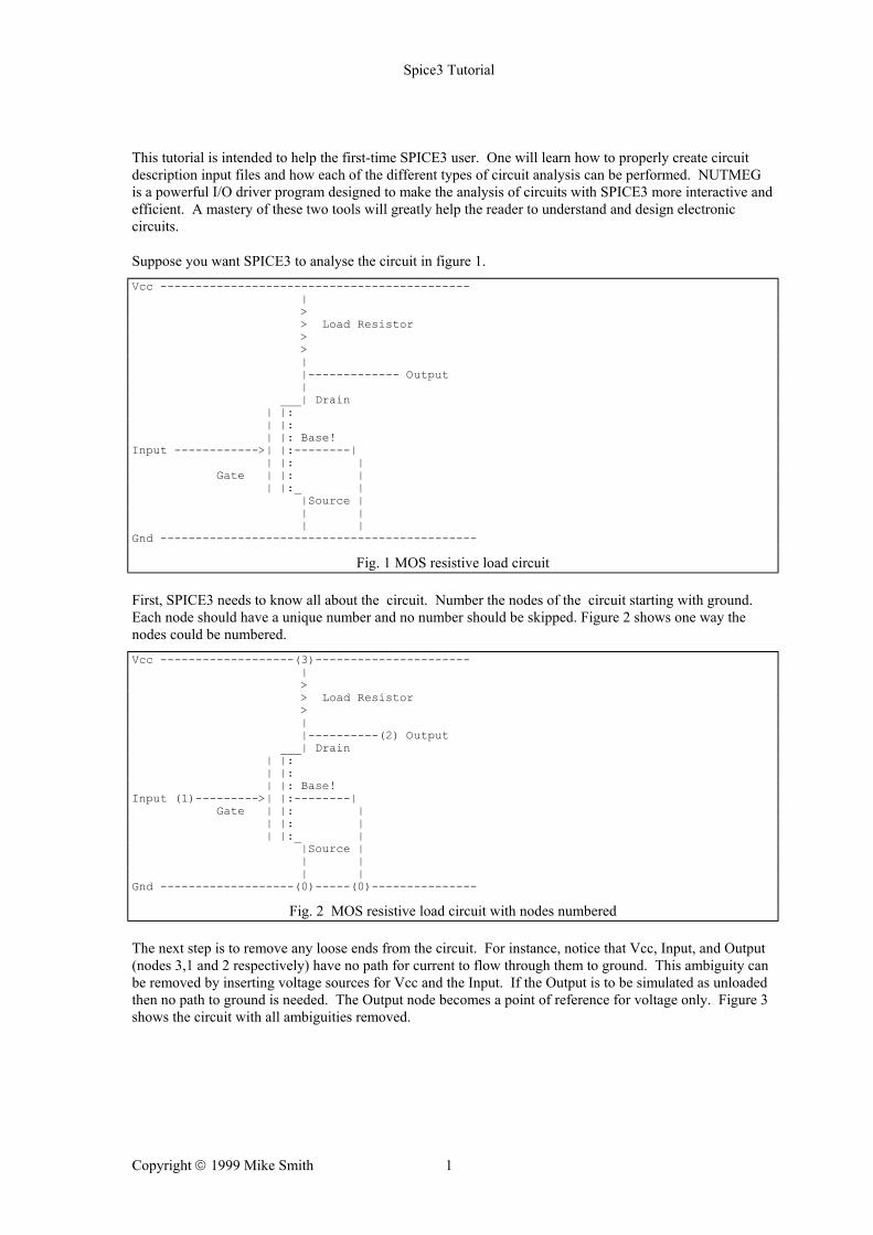
Suppose you want SPICE3 to analyse the circuit in figure 1. Vcc -------------------------------------------- | > > Load Resistor > > | |------------- Output | ___| Drain | |: | |: | |: Base! Input ------------>| |:--------| | |: | Gate | |: | | |:_ | |Source | | | | | Gnd ---------------------------------------------

Fig. 1 MOS resistive load circuit

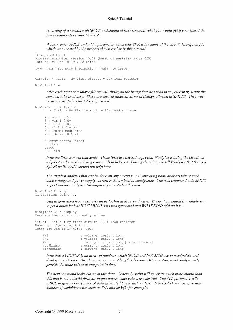
First, SPICE3 needs to know all about the circuit. Number the nodes of the circuit starting with ground. Each node should have a unique number and no number should be skipped. Figure 2 shows one way the nodes could be numbered. Vcc -------------------(3)---------------------- | > > Load Resistor > | |----------(2) Output ___| Drain | |: | |: | |: Base! Input (1)--------->| |:--------| Gate | |: | | |: | | |:_ | |Source | | | | | Gnd -------------------(0)-----(0)---------------

Fig. 2 MOS resistive load circuit with nodes numbered

The next step is to remove any loose ends from the circuit. For instance, notice that Vcc, Input, and Output (nodes 3,1 and 2 respectively) have no path for current to flow through them to ground. This ambiguity can be removed by inserting voltage sources for Vcc and the Input. If the Output is to be simulated as unloaded then no path to ground is needed. The Output node becomes a point of reference for voltage only. Figure 3 shows the circuit with all ambiguities removed.


Spice3 Tutorial

-------- Vcc -------------------(3)--------------- | | | ! | > | Load Resistor! | > | ! | > | | | (2) ......... Output! | | | ___| Drain + | |: Vcc | |: - | |: Base) | -- Input (1)------->| |:--------| | | Gate | |: | | | | |: | | | | |:_ | | + |Source | | Vin | | | - | | | | | | -------- Gnd -------------------(0)---(0)----------

Fig. 3 MOS resistive load circuit with loops closed

Choosing these values...

Vcc = 5v Vin = 0v Load = 10k ohms Gate = standard N-MOS gate. (SPICE3 default)

one is now ready to convert each device and supply in the circuit into a descriptive command for SPICE3. See the SPICE3 quick-reference card or users manual for an explanation of all device descriptions.

Vcc Vcc 3 0 5v 5 volts from node 3 to 0

Vin Vin 1 0 0v 0 volts from node 1 to 0

Load R1 3 2 10k 10k ohms from node 3 to 2

gate M1 2 1 0 0 modn a MOS gate over nodes 2,1 and 0

.model modn nmos the gate is NMOS with default parameters

With a text editor a file called "test1" can be created as shown below. * Title : My first circuit - 10k load resistor Vcc 3 0 5v Vin 1 0 0v R1 3 2 10k M1 2 1 0 0 modn .model modn nmos .DC Vin 0 5 .1

SPICE3 has some quirks since it is constantly improving. One of these is the inability for it to do DC analysis on a circuit unless the analysis is specified in the source. That is what the .dc card is for.

An example session with SPICE3 starting with this circuit appears below. User input is in normal type and added comments are in italics. SPICE3 run script

At this point we are at the command prompt. This tutorial assumes that your environment PATH variable is properly set so that spice3 is accessible. Note that your version of SPICE may not be named the same, nor work exactly the same as this example. This text however, is an actual script


Spice3 Tutorial

recording of a session with SPICE and should closely resemble what you would get if you/ issued the same commands at your terminal.

We now enter SPICE and add a parameter which tells SPICE the name of the circuit description file which was created by the process shown earlier in this tutorial.

1> wspice3 test1 Program: WinSpice, version: 0.01 (based on Berkeley Spice 3f5) Date built: Jan 5 1997 22:04:53 Type "help" for more information, "quit" to leave. Circuit: * Title : My first circuit - 10k load resistor WinSpice3 1 ->

After each input of a source file we will show you the listing that was read in so you can try using the same circuits used here. There are several different forms of listings allowed in SPICE3. They will be demonstrated as the tutorial proceeds.

WinSpice3 1 -> listing * Title : My first circuit - 10k load resistor 2 : vcc 3 0 5v 3 : vin 1 0 0v 4 : r1 3 2 10k 5 : m1 2 1 0 0 modn 6 : .model modn nmos 7 : .dc vin 0 5 .1 * Dummy control block .control .endc 9 : .end

Note the lines .control and .endc. These lines are needed to prevent WinSpice treating the circuit as a Spice2 netlist and inserting commands to help out. Putting these lines in tell WinSpice that this is a Spice3 netlist and it should not help here.

The simplest analysis that can be done on any circuit is DC operating point analysis where each node voltage and power supply current is determined at steady state. The next command tells SPICE to perform this analysis. No output is generated at this time.

WinSpice3 2 -> op DC Operating Point ...

Output generated from analysis can be looked at in several ways. The next command is a simple way to get a quick look at HOW MUCH data was generated and WHAT KIND of data it is.

WinSpice3 3 -> display Here are the vectors currently active: Title: * Title : My first circuit - 10k load resistor Name: op1 (Operating Point) Date: Thu Jan 16 15:40:44 1997 V(1) : voltage, real, 1 long V(2) : voltage, real, 1 long V(3) : voltage, real, 1 long [default scale] vcc#branch : current, real, 1 long vin#branch : current, real, 1 long

Note that a VECTOR is an array of numbers which SPICE and NUTMEG use to manipulate and display circuit data. The above vectors are of length 1 because DC operating point analysis only provide the node values at one point in time.

The next command looks closer at this data. Generally, print will generate much more output than this and is not a useful form for output unless exact values are desired. The ALL parameter tells SPICE to give us every piece of data generated by the last analysis. One could have specified any number of variable names such as V(1) and/or V(2) for example.


Spice3 Tutorial

WinSpice3 4 -> print all

The numbers here are node voltages. v(1) = 0.000000e+00 v(2) = 5.000000e+00 v(3) = 5.000000e+00

The numbers here are branch currents which correspond to the voltage supplies named. vcc#branch = -6.93317e-12 vin#branch = 0.000000e+00

Note that the source listing above contained a .DC card. This specifies a DC TRANSFER CURVE analysis which is useful for determining such things as fan-out or biasing for peak gain. To perform the analysis specified in the input file, a RUN command can be issued. Before a run can be done however, the circuit must be reset to allow another RUN on the circuit.

This terminology may be confusing. When a source file is read in, only the circuit topology is processed. This allows a variety of interactive analysis to then be performed without having to re-read the entire circuit. Any analysis can be thought of as running a program that puts the selected circuit through its paces.

WinSpice3 5 -> reset WinSpice3 6 -> run

The run in this case was equivalent to issuing a

dc vin 0 5 .1

directly because this was the analysis specified in the input deck (file). If we now issue a LET command without any parameter, all the vector variables will be printed out. This is exactly like a display command but shorter.

WinSpice3 8 -> let Here are the vectors currently active: Title: * Title : My first circuit - 10k load resistor Name: dc1 (DC transfer characteristic) Date: Thu Jan 16 15:42:38 1997 V(1) : voltage, real, 51 long V(2) : voltage, real, 51 long V(3) : voltage, real, 51 long sweep : voltage, real, 51 long [default scale] vcc#branch : current, real, 51 long vin#branch : current, real, 51 long

Note that these vectors are each 51 members long. This is because 5/.1 = 50 separate voltage points plus the terminating point. Note that vin is the scale. This is because the .DC card specified vin as the changing voltage which drives the rest of the circuit.

This much data is best understood in the form of a plot. NUTMEG, the front end for SPICE, allows a wide variety of plots to be done and can take advantage of graphics terminals and plotters. To use these graphics capabilities, one needs a graphics terminal and the TERM and DISPLAY UNIX environment variables properly set. See the NUTMEG users guide for details.

In order to maintain portability and printability of this document, only the asciiplot command is used. This allows users to see data on any terminal.

The following commands set some of the many SPICE/NUTMEG environment variables so that plot output will conform to a standard page size.

WinSpice3 -> set width=80 WinSpice3 -> set height=66


Spice3 Tutorial

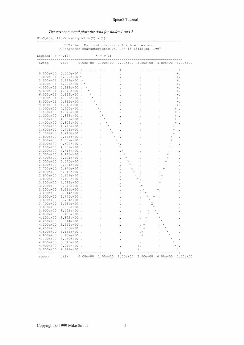
The next command plots the data for nodes 1 and 2. WinSpice3 11 -> asciiplot v(2) v(1) -------------------------------------------------------------------------- * Title : My first circuit - 10k load resistor DC transfer characteristic Thu Jan 16 15:42:38 1997 Legend: + = v(2) * = v(1) -------------------------------------------------------------------------- sweep v(2) 0.00e+00 1.00e+00 2.00e+00 3.00e+00 4.00e+00 5.00e+00 ----------------------|---------|---------|---------|---------|---------| 0.000e+00 5.000e+00 * . . . . +. 1.000e-01 4.999e+00 * . . . . +. 2.000e-01 4.996e+00 .* . . . . +. 3.000e-01 4.991e+00 . * . . . . +. 4.000e-01 4.984e+00 . * . . . . +. 5.000e-01 4.975e+00 . * . . . . +. 6.000e-01 4.964e+00 . * . . . . +. 7.000e-01 4.951e+00 . * . . . . +. 8.000e-01 4.936e+00 . * . . . . +. 9.000e-01 4.919e+00 . * . . . . +. 1.000e+00 4.900e+00 . *. . . . + . 1.100e+00 4.879e+00 . * . . . + . 1.200e+00 4.856e+00 . .* . . . + . 1.300e+00 4.831e+00 . . * . . . + . 1.400e+00 4.804e+00 . . * . . . + . 1.500e+00 4.775e+00 . . * . . . + . 1.600e+00 4.744e+00 . . * . . . + . 1.700e+00 4.711e+00 . . * . . . + . 1.800e+00 4.676e+00 . . * . . . + . 1.900e+00 4.639e+00 . . * . . . + . 2.000e+00 4.600e+00 . . *. . . + . 2.100e+00 4.559e+00 . . * . . + . 2.200e+00 4.516e+00 . . .* . . + . 2.300e+00 4.471e+00 . . . * . . + . 2.400e+00 4.424e+00 . . . * . . + . 2.500e+00 4.375e+00 . . . * . . + . 2.600e+00 4.324e+00 . . . * . . + . 2.700e+00 4.271e+00 . . . * . . + . 2.800e+00 4.216e+00 . . . * . . + . 2.900e+00 4.159e+00 . . . * . .+ . 3.000e+00 4.100e+00 . . . *. + . 3.100e+00 4.039e+00 . . . * + . 3.200e+00 3.976e+00 . . . .* +. . 3.300e+00 3.911e+00 . . . . * +. . 3.400e+00 3.844e+00 . . . . * + . . 3.500e+00 3.775e+00 . . . . * + . . 3.600e+00 3.704e+00 . . . . * + . . 3.700e+00 3.631e+00 . . . . X . . 3.800e+00 3.562e+00 . . . . + * . . 3.900e+00 3.495e+00 . . . . + * . . 4.000e+00 3.432e+00 . . . . + *. . 4.100e+00 3.372e+00 . . . . + * . 4.200e+00 3.314e+00 . . . . + .* . 4.300e+00 3.259e+00 . . . . + . * . 4.400e+00 3.206e+00 . . . . + . * . 4.500e+00 3.156e+00 . . . .+ . * . 4.600e+00 3.107e+00 . . . .+ . * . 4.700e+00 3.060e+00 . . . + . * . 4.800e+00 3.015e+00 . . . + . * . 4.900e+00 2.971e+00 . . . +. . * . 5.000e+00 2.929e+00 . . . +. . *. ----------------------|---------|---------|---------|---------|---------| sweep v(2) 0.00e+00 1.00e+00 2.00e+00 3.00e+00 4.00e+00 5.00e+00


Spice3 Tutorial

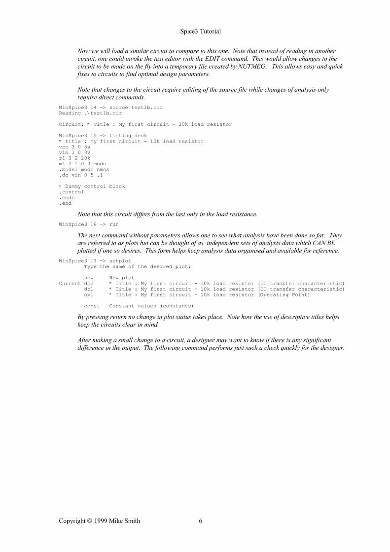
Now we will load a similar circuit to compare to this one. Note that instead of reading in another circuit, one could invoke the text editor with the EDIT command. This would allow changes to the circuit to be made on the fly into a temporary file created by NUTMEG. This allows easy and quick fixes to circuits to find optimal design parameters.

Note that changes to the circuit require editing of the source file while changes of analysis only require direct commands.

WinSpice3 14 -> source test1b.cir Reading .\test1b.cir Circuit: * Title : My first circuit - 20k load resistor WinSpice3 15 -> listing deck * title : my first circuit - 10k load resistor vcc 3 0 5v vin 1 0 0v r1 3 2 20k m1 2 1 0 0 modn .model modn nmos .dc vin 0 5 .1 * Dummy control block .control .endc .end

Note that this circuit differs from the last only in the load resistance. WinSpice3 16 -> run

The next command without parameters allows one to see what analysis have been done so far. They are referred to as plots but can be thought of as independent sets of analysis data which CAN BE plotted if one so desires. This form helps keep analysis data organised and available for reference.

WinSpice3 17 -> setplot Type the name of the desired plot: new New plot Current dc2 * Title : My first circuit - 10k load resistor (DC transfer characteristic) dc1 * Title : My first circuit - 10k load resistor (DC transfer characteristic) op1 * Title : My first circuit - 10k load resistor (Operating Point) const Constant values (constants)

By pressing return no change in plot status takes place. Note how the use of descriptive titles helps keep the circuits clear in mind.

After making a small change to a circuit, a designer may want to know if there is any significant difference in the output. The following command performs just such a check quickly for the designer.


Spice3 Tutorial

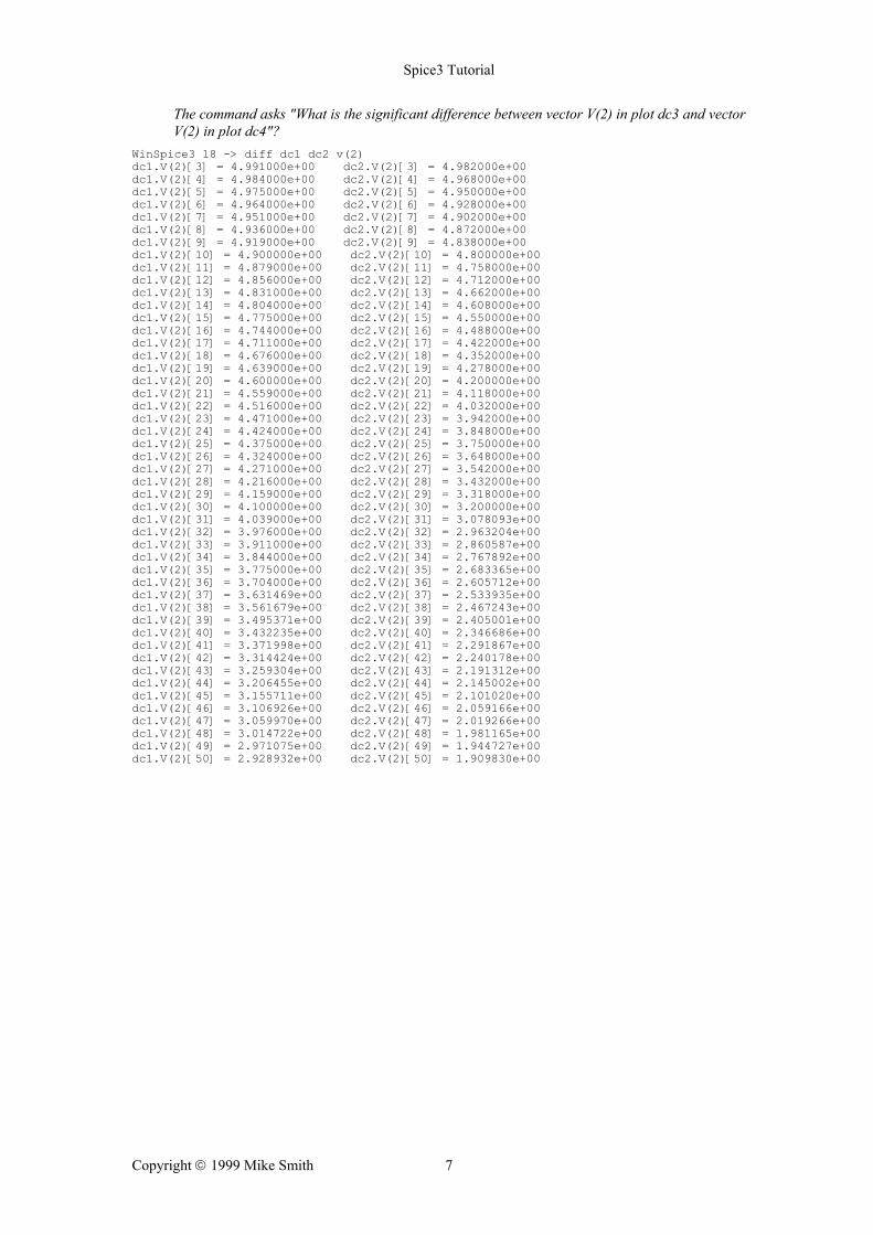
The command asks "What is the significant difference between vector V(2) in plot dc3 and vector V(2) in plot dc4"?

WinSpice3 18 -> diff dc1 dc2 v(2) dc1.V(2)[3] = 4.991000e+00 dc2.V(2)[3] = 4.982000e+00 dc1.V(2)[4] = 4.984000e+00 dc2.V(2)[4] = 4.968000e+00 dc1.V(2)[5] = 4.975000e+00 dc2.V(2)[5] = 4.950000e+00 dc1.V(2)[6] = 4.964000e+00 dc2.V(2)[6] = 4.928000e+00 dc1.V(2)[7] = 4.951000e+00 dc2.V(2)[7] = 4.902000e+00 dc1.V(2)[8] = 4.936000e+00 dc2.V(2)[8] = 4.872000e+00 dc1.V(2)[9] = 4.919000e+00 dc2.V(2)[9] = 4.838000e+00 dc1.V(2)[10] = 4.900000e+00 dc2.V(2)[10] = 4.800000e+00 dc1.V(2)[11] = 4.879000e+00 dc2.V(2)[11] = 4.758000e+00 dc1.V(2)[12] = 4.856000e+00 dc2.V(2)[12] = 4.712000e+00 dc1.V(2)[13] = 4.831000e+00 dc2.V(2)[13] = 4.662000e+00 dc1.V(2)[14] = 4.804000e+00 dc2.V(2)[14] = 4.608000e+00 dc1.V(2)[15] = 4.775000e+00 dc2.V(2)[15] = 4.550000e+00 dc1.V(2)[16] = 4.744000e+00 dc2.V(2)[16] = 4.488000e+00 dc1.V(2)[17] = 4.711000e+00 dc2.V(2)[17] = 4.422000e+00 dc1.V(2)[18] = 4.676000e+00 dc2.V(2)[18] = 4.352000e+00 dc1.V(2)[19] = 4.639000e+00 dc2.V(2)[19] = 4.278000e+00 dc1.V(2)[20] = 4.600000e+00 dc2.V(2)[20] = 4.200000e+00 dc1.V(2)[21] = 4.559000e+00 dc2.V(2)[21] = 4.118000e+00 dc1.V(2)[22] = 4.516000e+00 dc2.V(2)[22] = 4.032000e+00 dc1.V(2)[23] = 4.471000e+00 dc2.V(2)[23] = 3.942000e+00 dc1.V(2)[24] = 4.424000e+00 dc2.V(2)[24] = 3.848000e+00 dc1.V(2)[25] = 4.375000e+00 dc2.V(2)[25] = 3.750000e+00 dc1.V(2)[26] = 4.324000e+00 dc2.V(2)[26] = 3.648000e+00 dc1.V(2)[27] = 4.271000e+00 dc2.V(2)[27] = 3.542000e+00 dc1.V(2)[28] = 4.216000e+00 dc2.V(2)[28] = 3.432000e+00 dc1.V(2)[29] = 4.159000e+00 dc2.V(2)[29] = 3.318000e+00 dc1.V(2)[30] = 4.100000e+00 dc2.V(2)[30] = 3.200000e+00 dc1.V(2)[31] = 4.039000e+00 dc2.V(2)[31] = 3.078093e+00 dc1.V(2)[32] = 3.976000e+00 dc2.V(2)[32] = 2.963204e+00 dc1.V(2)[33] = 3.911000e+00 dc2.V(2)[33] = 2.860587e+00 dc1.V(2)[34] = 3.844000e+00 dc2.V(2)[34] = 2.767892e+00 dc1.V(2)[35] = 3.775000e+00 dc2.V(2)[35] = 2.683365e+00 dc1.V(2)[36] = 3.704000e+00 dc2.V(2)[36] = 2.605712e+00 dc1.V(2)[37] = 3.631469e+00 dc2.V(2)[37] = 2.533935e+00 dc1.V(2)[38] = 3.561679e+00 dc2.V(2)[38] = 2.467243e+00 dc1.V(2)[39] = 3.495371e+00 dc2.V(2)[39] = 2.405001e+00 dc1.V(2)[40] = 3.432235e+00 dc2.V(2)[40] = 2.346686e+00 dc1.V(2)[41] = 3.371998e+00 dc2.V(2)[41] = 2.291867e+00 dc1.V(2)[42] = 3.314424e+00 dc2.V(2)[42] = 2.240178e+00 dc1.V(2)[43] = 3.259304e+00 dc2.V(2)[43] = 2.191312e+00 dc1.V(2)[44] = 3.206455e+00 dc2.V(2)[44] = 2.145002e+00 dc1.V(2)[45] = 3.155711e+00 dc2.V(2)[45] = 2.101020e+00 dc1.V(2)[46] = 3.106926e+00 dc2.V(2)[46] = 2.059166e+00 dc1.V(2)[47] = 3.059970e+00 dc2.V(2)[47] = 2.019266e+00 dc1.V(2)[48] = 3.014722e+00 dc2.V(2)[48] = 1.981165e+00 dc1.V(2)[49] = 2.971075e+00 dc2.V(2)[49] = 1.944727e+00 dc1.V(2)[50] = 2.928932e+00 dc2.V(2)[50] = 1.909830e+00


Spice3 Tutorial

It looks as though there was indeed a significant difference! With another quick edit session another circuit is created and read in as follows:

WinSpice3 19 -> source test1c.cir Reading .\test1c.cir NOTE: Spice3 commands found in input file. Circuit: * Title : My first circuit - 30k load resistor WinSpice3 20 -> listing logical * Title : My first circuit - 30k load resistor 2 : vcc 3 0 5v 3 : vin 1 0 0v 4 : r1 3 2 30k 5 : m1 2 1 0 0 modn 6 : .model modn nmos 7 : .dc vin 0 5 .1 9 : .control 10 : .endc 12 : .end WinSpice3 21 -> run WinSpice3 22 -> setplot WinSpice3 19 -> source test1c.cir Reading .\test1c.cir Circuit: * Title : My first circuit - 30k load resistor WinSpice3 20 -> listing logical * Title : My first circuit - 30k load resistor 2 : vcc 3 0 5v 3 : vin 1 0 0v 4 : r1 3 2 30k 5 : m1 2 1 0 0 modn 6 : .model modn nmos 7 : .dc vin 0 5 .1 9 : .control 10 : .endc 12 : .end WinSpice3 21 -> run WinSpice3 22 -> setplot Type the name of the desired plot: new New plot Current dc3 * Title : My first circuit - 30k load resistor (DC transfer characteristic) dc2 * Title : My first circuit - 10k load resistor (DC transfer characteristic) dc1 * Title : My first circuit - 10k load resistor (DC transfer characteristic) op1 * Title : My first circuit - 10k load resistor (Operating Point) const Constant values (constants) ?new

Now a new plot is set a current. This gives the user a clean slate to work with. We now use LET commands to bring in vectors from other analysis to create a comparison plot.

WinSpice3 23 -> let input = dc1.v(1) WinSpice3 24 -> let out10k = dc1.v(2) WinSpice3 25 -> let out20k = dc2.v(2) WinSpice3 26 -> let out30k = dc3.v(2) WinSpice3 27 -> let Here are the vectors currently active: Title: Anonymous Name: unknown3 (unknown) Date: Thu Jan 16 16:10:08 1997 input : voltage, real, 51 long [default scale] out10k : voltage, real, 51 long out20k : voltage, real, 51 long out30k : voltage, real, 51 long


Spice3 Tutorial

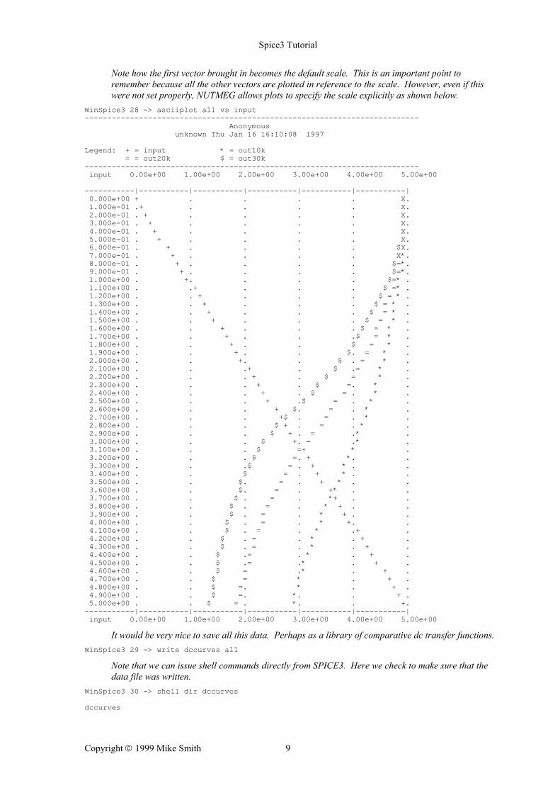
Note how the first vector brought in becomes the default scale. This is an important point to remember because all the other vectors are plotted in reference to the scale. However, even if this were not set properly, NUTMEG allows plots to specify the scale explicitly as shown below.

WinSpice3 28 -> asciiplot all vs input -------------------------------------------------------------------------- Anonymous unknown Thu Jan 16 16:10:08 1997 Legend: + = input * = out10k = = out20k $ = out30k -------------------------------------------------------------------------- input 0.00e+00 1.00e+00 2.00e+00 3.00e+00 4.00e+00 5.00e+00 -----------|-----------|-----------|-----------|-----------|-----------| 0.000e+00 + . . . . X. 1.000e-01 .+ . . . . X. 2.000e-01 . + . . . . X. 3.000e-01 . + . . . . X. 4.000e-01 . + . . . . X. 5.000e-01 . + . . . . X. 6.000e-01 . + . . . . $X. 7.000e-01 . + . . . . X*. 8.000e-01 . + . . . . $=*. 9.000e-01 . + . . . . $=*. 1.000e+00 . +. . . . $=* . 1.100e+00 . .+ . . . $ =* . 1.200e+00 . . + . . . $ = * . 1.300e+00 . . + . . . $ = * . 1.400e+00 . . + . . . $ = * . 1.500e+00 . . + . . . $ = * . 1.600e+00 . . + . . . $ = * . 1.700e+00 . . + . . .$ = * . 1.800e+00 . . + . . $ = * . 1.900e+00 . . + . . $. = * . 2.000e+00 . . +. . $ . = * . 2.100e+00 . . .+ . $ .= * . 2.200e+00 . . . + . $ = * . 2.300e+00 . . . + . $ =. * . 2.400e+00 . . . + . $ = . * . 2.500e+00 . . . + .$ = . * . 2.600e+00 . . . + $. = . * . 2.700e+00 . . . +$ . = . * . 2.800e+00 . . . $ + . = . * . 2.900e+00 . . . $ + . = .* . 3.000e+00 . . . $ +. = .* . 3.100e+00 . . . $ =+ * . 3.200e+00 . . . $ =. + *. . 3.300e+00 . . .$ = . + * . . 3.400e+00 . . $ = . + * . . 3.500e+00 . . $. = . + * . . 3.600e+00 . . $. = . +* . . 3.700e+00 . . $ . = . *+ . . 3.800e+00 . . $ . = . * + . . 3.900e+00 . . $ . = . * + . . 4.000e+00 . . $ . = . * +. . 4.100e+00 . . $ . = . * .+ . 4.200e+00 . . $ . = . * . + . 4.300e+00 . . $ . = . * . + . 4.400e+00 . . $ .= . * . + . 4.500e+00 . . $ .= .* . + . 4.600e+00 . . $ = .* . + . 4.700e+00 . . $ = * . + . 4.800e+00 . . $ =. * . + . 4.900e+00 . . $ =. *. . + . 5.000e+00 . . $ = . *. . +. -----------|-----------|-----------|-----------|-----------|-----------| input 0.00e+00 1.00e+00 2.00e+00 3.00e+00 4.00e+00 5.00e+00

It would be very nice to save all this data. Perhaps as a library of comparative dc transfer functions. WinSpice3 29 -> write dccurves all

Note that we can issue shell commands directly from SPICE3. Here we check to make sure that the data file was written.

WinSpice3 30 -> shell dir dccurves dccurves


Spice3 Tutorial

To demonstrate how these data files are recovered, we now quit SPICE3 and reenter the program. This also has the added feature of allowing all previous unwanted data do be discarded which might otherwise be filling up disk/memory space.

WinSpice3 31 -> quit Warning: the following plots haven't been saved: dc3 * Title : My first circuit - 30k load resistor, DC transfer characteristic dc2 * Title : My first circuit - 10k load resistor, DC transfer characteristic dc1 * Title : My first circuit - 10k load resistor, DC transfer characteristic op1 * Title : My first circuit - 10k load resistor, Operating Point Are you sure you want to quit (yes)?y c:\spice3> wspice3 Program: WinSpice, version: 0.01 (based on Berkeley Spice 3f5) Date built: Jan 5 1997 22:04:53 Type "help" for more information, "quit" to leave. WinSpice3 1 -> let Here are the vectors currently active: Title: Constant values Name: const (constants) Date: Sat Aug 16 10:55:15 PDT 1986 boltz : notype, real, 1 long c : notype, real, 1 long e : notype, real, 1 long echarge : notype, real, 1 long false : notype, real, 1 long i : notype, complex, 1 long kelvin : notype, real, 1 long no : notype, real, 1 long pi : notype, real, 1 long planck : notype, real, 1 long true : notype, real, 1 long yes : notype, real, 1 long [default scale] WinSpice3 2 -> load dccurves Loading raw data file ("dccurves") . . . done. Title: Anonymous Name: unknown Date: Thu Jan 16 16:10:08 1997 Here are the vectors currently active: Title: Anonymous Name: unknown1 (unknown) Date: Thu Jan 16 16:10:08 1997 input : voltage, real, 51 long [default scale] out10k : voltage, real, 51 long out20k : voltage, real, 51 long out30k : voltage, real, 51 long

Let us now proceed on to some more interesting circuits and analysis. WinSpice3 3 -> source test2.cir


Spice3 Tutorial

Note that a physical listing produces almost an exact replica of the source file numbered for us. Reading .\test2.cir Circuit: * Cmos inverter WinSpice3 4 -> listing physical * Cmos inverter 1 : * cmos inverter 2 : vcc 3 0 5v 3 : vin 1 0 0v 4 : m1 2 1 0 0 modn 5 : m2 3 1 2 3 modp 6 : .model modp pmos 7 : .model modn nmos 8 : .dc vin 0 5 .1 9 : * dummy control block 10 : .control 11 : .endc 13 : .end WinSpice3 5 -> run

Now we go to the comparison plot and add the CMOS dc transfer curve into our library of transfer curves.

WinSpice3 6 -> setplot Type the name of the desired plot: new New plot Current dc2 * Cmos inverter (DC transfer characteristic) unknown1 Anonymous (unknown) const Constant values (constants) ? unknown1 WinSpice3 7 -> let outCMOS = dc2.v(2)


Spice3 Tutorial

The width and height variables must be respecified since this is a new run. This could be avoided if a .spiceinit file were prepaired which would automatically be read in and processed as SPICE3 starts up.

WinSpice3 8 -> set width=80 WinSpice3 9 -> set height=66 WinSpice3 10 -> asciiplot all vs input -------------------------------------------------------------------------- Anonymous unknown Thu Jan 16 16:10:08 1997 Legend: + = input * = out10k = = out20k $ = out30k % = outCMOS -------------------------------------------------------------------------- input -1.00e+00 0.00e+00 1.00e+00 2.00e+00 3.00e+00 4.00e+00 5.00e+00 -----------|---------|---------|---------|---------|---------|---------| 0.000e+00 . + . . . . X. 1.000e-01 . + . . . . X. 2.000e-01 . .+ . . . . X. 3.000e-01 . . + . . . . X. 4.000e-01 . . + . . . . X. 5.000e-01 . . + . . . . X. 6.000e-01 . . + . . . . $X. 7.000e-01 . . + . . . . $X. 8.000e-01 . . + . . . . XX. 9.000e-01 . . + . . . . $=X. 1.000e+00 . . +. . . . $=X . 1.100e+00 . . + . . . $=X . 1.200e+00 . . .+ . . . $ =X . 1.300e+00 . . . + . . . $ =%* . 1.400e+00 . . . + . . . $ =%* . 1.500e+00 . . . + . . . $ =%* . 1.600e+00 . . . + . . . $ = %* . 1.700e+00 . . . + . . .$ =% * . 1.800e+00 . . . + . . $ =% * . 1.900e+00 . . . + . . $. =% * . 2.000e+00 . . . +. . $ .=% * . 2.100e+00 . . . + . $ .X * . 2.200e+00 . . . .+ . $ %= * . 2.300e+00 . . . . + . $ % =. * . 2.400e+00 . . . . + . $ % = . * . 2.500e+00 . . . . +% .$ = . * . 2.600e+00 . . . % . + $. = . * . 2.700e+00 . . . % . + $ . = . * . 2.800e+00 . . % . $+ . = . * . 2.900e+00 . . % . . $ + . = .* . 3.000e+00 . . % . . $ +.= * . 3.100e+00 . . % . . $ X * . 3.200e+00 . . % . . $ =.+ *. . 3.300e+00 . . % . .$ = . + *. . 3.400e+00 . . % . $ = . + * . . 3.500e+00 . . % . $. = . + * . . 3.600e+00 . . % . $. = . + * . . 3.700e+00 . . % . $ . = . X . . 3.800e+00 . .% . $ . = . * + . . 3.900e+00 . .% . $ . = . * + . . 4.000e+00 . .% . $ . = . * +. . 4.100e+00 . % . $ . = . * + . 4.200e+00 . % . $ . = . * .+ . 4.300e+00 . % . $ .= . * . + . 4.400e+00 . % . $ .= . * . + . 4.500e+00 . % . $ .= .* . + . 4.600e+00 . % . $ = .* . + . 4.700e+00 . % . $ = * . + . 4.800e+00 . % . $ =. * . + . 4.900e+00 . % . $ =. *. . + . 5.000e+00 . %. . $ =. *. . +. -----------|---------|---------|---------|---------|---------|---------| input -1.00e+00 0.00e+00 1.00e+00 2.00e+00 3.00e+00 4.00e+00 5.00e+00


Spice3 Tutorial

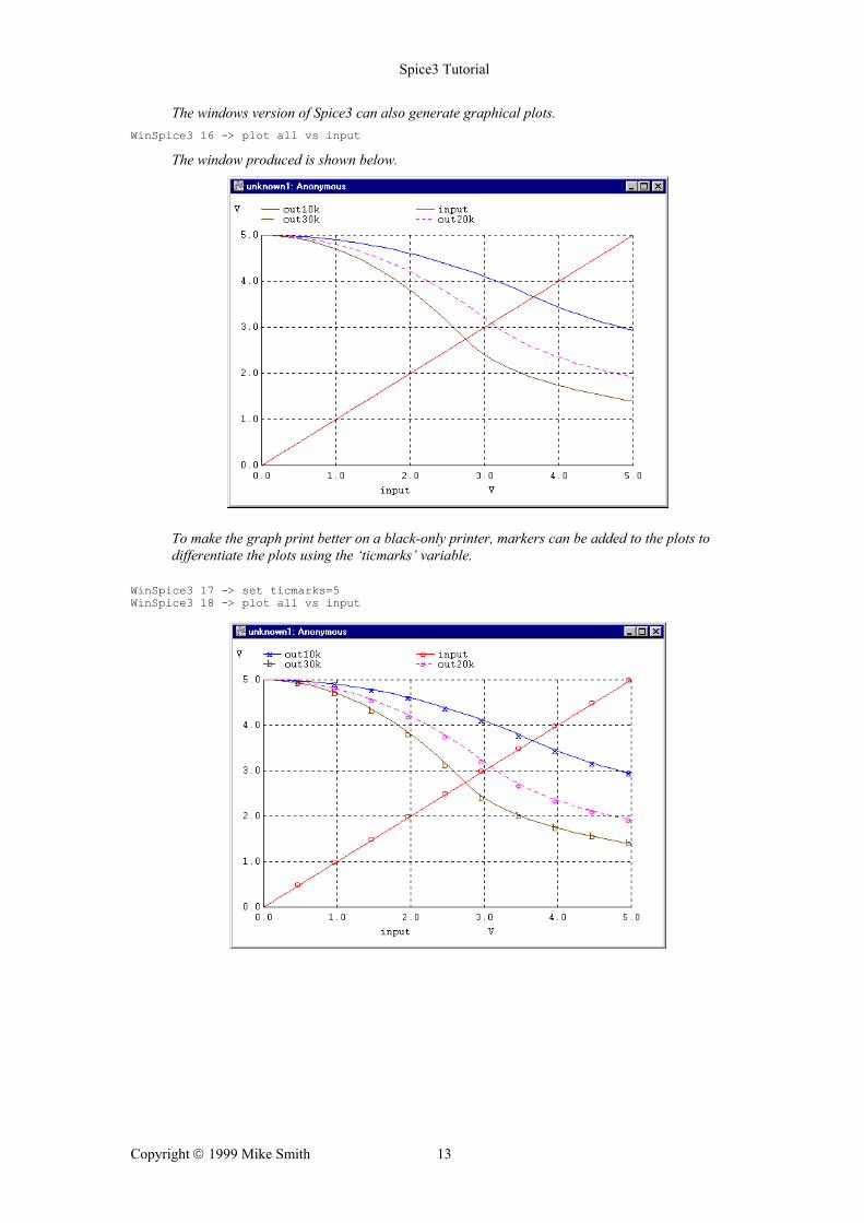
The windows version of Spice3 can also generate graphical plots. WinSpice3 16 -> plot all vs input

The window produced is shown below.

To make the graph print better on a black-only printer, markers can be added to the plots to differentiate the plots using the ‘ticmarks’ variable.

WinSpice3 17 -> set ticmarks=5 WinSpice3 18 -> plot all vs input


Spice3 Tutorial

This next circuit makes the CMOS circuit a subcircuit which can be used as a piece of a much larger circuit.

WinSpice3 17 ->source test3.cir WinSpice3 18 ->listing logical * Title : My first sub-circuit, 4 : .subckt invert 1 2 3 4 5 : m2 4 2 3 4 modp 6 : m1 3 2 1 1 modn 7 : .ends 8 : vcc 3 0 5v 9 : vin 1 0 pulse(0 5 0 .1ns .1ns 20ns 40ns) 10 : x1 0 1 2 3 invert 11 : x2 0 2 4 3 invert 12 : x3 0 4 5 3 invert 13 : c1 5 0 1pf 14 : .model modn nmos 15 : .model modp pmos 16 : .dc vin 0 5 .1 18 : .control 19 : .endc 21 : .end WinSpice3 19 -> listing expand * Title : My first sub-circuit, 8 : vcc 3 0 5v 9 : vin 1 0 pulse(0 5 0 .1ns .1ns 20ns 40ns) 5 : m:x1:2 3 1 2 3 modp 6 : m:x1:1 2 1 0 0 modn 5 : m:x2:2 3 2 4 3 modp 6 : m:x2:1 4 2 0 0 modn 5 : m:x3:2 3 4 5 3 modp 6 : m:x3:1 5 4 0 0 modn 13 : c1 5 0 1pf 14 : .model modn nmos 15 : .model modp pmos 16 : .dc vin 0 5 .1 18 : .end

Note the difference in the listings. The second one shows how SPICE sees the circuit once the subcircuits have been expanded.

WinSpice3 20 -> run Warning: vin: no DC value, transient time 0 value used


Spice3 Tutorial

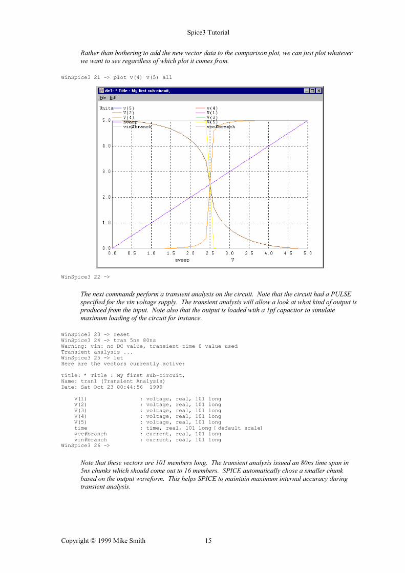
Rather than bothering to add the new vector data to the comparison plot, we can just plot whatever we want to see regardless of which plot it comes from.

WinSpice3 21 -> plot v(4) v(5) all

WinSpice3 22 ->

The next commands perform a transient analysis on the circuit. Note that the circuit had a PULSE specified for the vin voltage supply. The transient analysis will allow a look at what kind of output is produced from the input. Note also that the output is loaded with a 1pf capacitor to simulate maximum loading of the circuit for instance.

WinSpice3 23 -> reset WinSpice3 24 -> tran 5ns 80ns Warning: vin: no DC value, transient time 0 value used Transient analysis ... WinSpice3 25 -> let Here are the vectors currently active: Title: * Title : My first sub-circuit, Name: tran1 (Transient Analysis) Date: Sat Oct 23 00:44:56 1999 V(1) : voltage, real, 101 long V(2) : voltage, real, 101 long V(3) : voltage, real, 101 long V(4) : voltage, real, 101 long V(5) : voltage, real, 101 long time : time, real, 101 long [default scale] vcc#branch : current, real, 101 long vin#branch : current, real, 101 long WinSpice3 26 ->

Note that these vectors are 101 members long. The transient analysis issued an 80ns time span in 5ns chunks which should come out to 16 members. SPICE automatically chose a smaller chunk based on the output waveform. This helps SPICE to maintain maximum internal accuracy during transient analysis.


Spice3 Tutorial

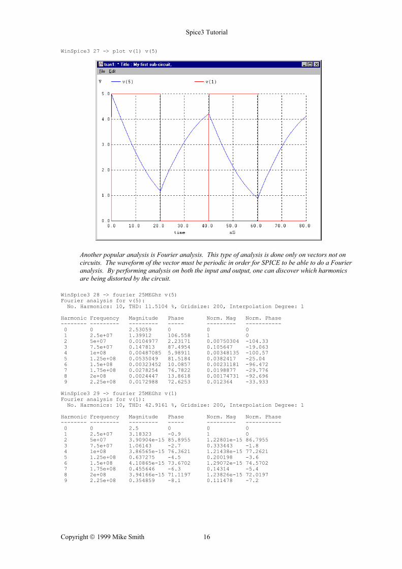
WinSpice3 27 -> plot v(1) v(5)

Another popular analysis is Fourier analysis. This type of analysis is done only on vectors not on circuits. The waveform of the vector must be periodic in order for SPICE to be able to do a Fourier analysis. By performing analysis on both the input and output, one can discover which harmonics are being distorted by the circuit.

WinSpice3 28 -> fourier 25MEGhz v(5) Fourier analysis for v(5): No. Harmonics: 10, THD: 11.5104 %, Gridsize: 200, Interpolation Degree: 1 Harmonic Frequency Magnitude Phase Norm. Mag Norm. Phase -------- --------- --------- ----- --------- ----------- 0 0 2.53059 0 0 0 1 2.5e+07 1.39912 106.558 1 0 2 5e+07 0.0104977 2.23171 0.00750304 -104.33 3 7.5e+07 0.147813 87.4954 0.105647 -19.063 4 1e+08 0.00487085 5.98911 0.00348135 -100.57 5 1.25e+08 0.0535049 81.5184 0.0382417 -25.04 6 1.5e+08 0.00323452 10.0857 0.00231181 -96.472 7 1.75e+08 0.0278254 76.7822 0.0198877 -29.776 8 2e+08 0.0024447 13.8618 0.00174731 -92.696 9 2.25e+08 0.0172988 72.6253 0.012364 -33.933 WinSpice3 29 -> fourier 25MEGhz v(1) Fourier analysis for v(1): No. Harmonics: 10, THD: 42.9161 %, Gridsize: 200, Interpolation Degree: 1 Harmonic Frequency Magnitude Phase Norm. Mag Norm. Phase -------- --------- --------- ----- --------- ----------- 0 0 2.5 0 0 0 1 2.5e+07 3.18323 -0.9 1 0 2 5e+07 3.90904e-15 85.8955 1.22801e-15 86.7955 3 7.5e+07 1.06143 -2.7 0.333443 -1.8 4 1e+08 3.86565e-15 76.3621 1.21438e-15 77.2621 5 1.25e+08 0.637275 -4.5 0.200198 -3.6 6 1.5e+08 4.10865e-15 73.6702 1.29072e-15 74.5702 7 1.75e+08 0.455646 -6.3 0.14314 -5.4 8 2e+08 3.94166e-15 71.1197 1.23826e-15 72.0197 9 2.25e+08 0.354859 -8.1 0.111478 -7.2


Spice3 Tutorial

The next circuit allows simple demonstration of small signal ac analysis. WinSpice3 30 -> source test4.cir Reading .\test4.cir Circuit: * Title: simple choke filter subcircuit - order 3 WinSpice3 31 -> listing deck * title: simple choke filter subcircuit - order 3 .subckt filter 1 2 * 1=input 2=output c1 1 2 1pf r1 2 0 1k .ends vin 1 0 ac 1v x1 1 2 filter x2 2 3 filter x3 3 4 filter x4 4 5 filter x5 5 6 filter x6 6 7 filter * dummy control block .control .endc .end WinSpice3 32 -> listing expand * Title: simple choke filter subcircuit - order 3 7 : vin 1 0 ac 1v 4 : c:x1:1 1 2 1pf 5 : r:x1:1 2 0 1k 4 : c:x2:1 2 3 1pf 5 : r:x2:1 3 0 1k 4 : c:x3:1 3 4 1pf 5 : r:x3:1 4 0 1k 4 : c:x4:1 4 5 1pf 5 : r:x4:1 5 0 1k 4 : c:x5:1 5 6 1pf 5 : r:x5:1 6 0 1k 4 : c:x6:1 6 7 1pf 5 : r:x6:1 7 0 1k 23 : .end WinSpice3 33 -> ac dec 5 1 10GHz Warning: vin: has no value, DC 0 assumed AC analysis ... WinSpice3 34 -> plot v(2) v(3) v(4) v(5) v(6) v(7) WinSpice3 35 ->


Spice3 Tutorial

Note here that the vectors v(2) etc are complex. WinSpice assumes that ‘plot v(2)’ means ‘plot mag(v(2))’ for complex vectors. To plot the complex vector in different ways, we can use ‘plot real(v(2))’ or ‘plot imag(v(2))’.

WinSpice3 35 ->plot real(v(2)) real(v(3)) real(v(4)) real(v(5)) real(v(6)) real(v(7))

By dragging a box with the mouse around the interesting part of the plot, a new plot window will be drawn which zooms in on the plot.

Notice the dotted box in the window.

The zoomed plot is drawn when the mouse is released.


Spice3 Tutorial

SPICE3 and NUTMEG provide many other facilities as well. These allow customising of the program to the user's needs. Some examples of these other features follow.

NUTMEG keeps track of the command history just like the UNIX C-Shell (csh). This allows the use of ! substitutions to repeat often typed commands.

WinSpice3 36 -> history 25 plot v(1) v(5) 26 fourier 25MEGhz v(5) 27 fourier 25MEGhz v(1) 28 cd 29 source test4.cir 30 listing deck 31 listing expand 32 ac dec 5 1 10GHz 33 plot v(2) v(3) v(4) v(5) v(6) v(7) 34 history WinSpice3 37 ->

After a long run SPICE3 may have begun to eat up a lot of resources. It is important that SPICE3 users try to minimise resource usage because circuit simulation requires LOTS of computer power and often degrades system performance if used wastefully. The following command helps a user keep track of resource usage.

WinSpice3 38 -> rusage elapsed time since last call: 3041.000 seconds. Total elapsed time: 3041.000 seconds. Current dynamic memory usage = 106418, Dynamic memory limit = 0. WinSpice3 39 ->

The above script is only an introduction. Circuit analysis is an art and SPICE, like any artist's tool has its own quirks which may sometimes seem strange to a new user. It is important that a user clearly understand what type of analysis he/she is trying to perform and why. A clear understanding of how SPICE works internally will also help considerably in understanding its quirks. Complicated circuits with such things as positive feedback can cause analysis to force non-convergence or even a floating point fault. In any case, SPICE allows the designer to try out his design before it is built.


Spice3 Tutorial

Simulation helps create understanding of circuits. Play with circuits. Explore the possibilities and see how well your understanding of circuits and SPICE is.

For more detailed information on SPICE see the SPICE users guide.


Documents

A Tutorial for Spice3 / Nutmeg - Universidad de Sevillaiecon02.us.es/ASIGN/DCSE_1IE/WinSpice_tutorial.pdf · gate M1 2 1 0 0 modn a MOS gate over nodes 2 ... nor work exactly the