A turbulent, high magnetic Reynolds number experimental model of Earth's core

Journal of Geophysical Research: Solid Earth

RESEARCH ARTICLE10.1002/2013JB010733

Key Points:• Many states in turbulent spherical

Couette flow depending onRossby number

• Transitions affect angularmomentum transport and internalfield generation

• Dynamo-like enhancement of appliedexternal dipole by nonaxisymmetricwaves

Correspondence to:D. P. Lathrop,[email protected]

Citation:Zimmerman, D. S., S. A. Triana, H.-C.Nataf, and D. P. Lathrop (2014), Aturbulent, high magnetic Reynoldsnumber experimental model of Earth’score, J. Geophys. Res. Solid Earth, 119,4538–4557, doi:10.1002/2013JB010733.

Received 30 SEP 2013

Accepted 22 MAY 2014

Accepted article online 28 MAY 2014

Published online 24 JUN 2014

A turbulent, high magnetic Reynolds number experimentalmodel of Earth’s coreDaniel S. Zimmerman1, Santiago Andrés Triana2, Henri-Claude Nataf3,4,5, and Daniel P. Lathrop6

1Institute for Research in Electronics and Applied Physics, University of Maryland, College Park, Maryland, USA, 2Institute ofAstronomy, KU Leuven, Leuven, Belgium, 3Université Grenoble Alpes, ISTerre, Grenoble, France, 4CNRS, ISTerre, Grenoble,France, 5IRD, ISTerre, Grenoble, France 6Physics, Geology, IREAP, IPST, University of Maryland, College Park, Maryland, USA

Abstract We present new experimental results from the University of Maryland Three MeterGeodynamo experiment. We drive a fully turbulent flow in water and also in sodium at magnetic Reynoldsnumber Rm = ΔΩ(ro − ri)2∕𝜂, up to 715 (about half design maximum) in a spherical Couette apparatusgeometrically similar to Earth’s core. We have not yet observed a self-generating dynamo, but we study MHDeffects with an externally applied axisymmetric magnetic field. We survey a broad range of Rossby number−68 < Ro = ΔΩ∕Ωo < 65 in both purely hydrodynamic water experiments and sodium experimentswith weak, nearly passive applied field. We characterize angular momentum transport and substantialgeneration of internal toroidal magnetic field (the Ω effect) as a function of Ro and find a rich dependence ofboth angular momentum transport and Ω effect on Ro. Internal azimuthal field generation peaks at Ro = 6with a gain as high as 9 with weak applied field. At this Rossby number, we also perform experiments withsignificant Lorentz forces by increasing the applied magnetic field. We observe a reduction of the Ω effect, alarge increase in angular momentum transport, and the onset of new dynamical states. The state we reachat maximum applied field shows substantial magnetic field gain in the axial dipole moment, enhancing theapplied dipole moment. This intermittent dipole enhancement must come from nonaxisymmetric flow andseems to be a geodynamo-style feedback involving differential rotation and large-scale drifting waves.

1. Introduction

The Earth’s main magnetic field arises from partially understood processes in the outer core. The magneticdynamo is thought to be driven by convective flows in the liquid iron outer core. One obstacle to quantita-tive modeling and prediction is turbulence. Estimates of the hydrodynamic Reynolds number, a measure ofnonlinearity in the flow, give Re = UL∕𝜈≈108, where U is the velocity scale inferred in the core, L the sizeof the core, and 𝜈 an estimate of a typical viscosity for the liquid iron in the outer core. In liquid metals, themagnetic diffusivity 𝜂 = 1∕(𝜇𝜎) is much higher than the viscosity, so that the magnetic Prandtl numberPrm = 𝜈∕𝜂 is very low (10−5 in the case of liquid sodium). Hydromagnetic flows of interest in geophysical andastrophysical situations have high magnetic Reynolds number Rm = UL∕𝜂, and the low magnetic Prandtlnumber implies that Re must be many orders of magnitude higher than Rm.

Direct numerical simulation becomes unfeasible with current computational tools not much above Re∼106

and requires high performance computing above Re∼105. Experimental models are useful because theyreach higher Reynolds number than any simulation and have significant levels of turbulence. However,diagnostic measurements of the flow are limited compared to numerical simulations.

The success of the Riga [Gailitis et al., 2001, 2008] and Karlsruhe [Stieglitz and Müller, 2001] experimentsdemonstrated that self-excitation was possible in fluid dynamo experiments and that theoretical pre-dictions for the dynamo onset of a well-organized flow were accurate. These pioneer experiments alsoopened the way to second generation experiments, which aimed at producing dynamo onset in highly tur-bulent flows. However, it was discovered that turbulent fluctuations tend to oppose the dynamo actionpredicted for the mean flow [Lathrop et al., 2001; Petrelis et al., 2003; Spence et al., 2006; Frick et al.,2010; Rahbarnia et al., 2012]. Nevertheless, the von Kármán Sodium experiment achieved self-excitedfield generation when ferromagnetic impellers are used, yielding a rich collection of dynamo behaviors[Monchaux et al., 2007; Berhanu et al., 2007; Monchaux et al., 2009; Berhanu et al., 2010].

ZIMMERMAN ET AL. ©2014. American Geophysical Union. All Rights Reserved. 4538

http://publications.agu.org/journals/

http://onlinelibrary.wiley.com/journal/10.1002/(ISSN)2169-9356

http://dx.doi.org/10.1002/2013JB010733

Journal of Geophysical Research: Solid Earth 10.1002/2013JB010733

Earth’s dynamo is peculiar because its magnetic energy, EM, is perhaps 4 orders of magnitude larger than thekinetic energy, EK, of the large-scale convective motions inferred from the secular variation of the magneticfield [e.g., Holme, 2007]. This feature (EM >> EK) is not yet reproduced in numerical simulations, and it is notclear how this arises.

In Earth’s core, the time scale for rotation (𝜏Ω = 1 day) is much shorter than the time scale of magnetic(Alfvén) waves (𝜏A ≃ 5 years), which have been recently discovered [Gillet et al., 2010]. As a consequence,motions are expected to be quasi-geostrophic on short time scales, while shaped by the magnetic field onlong time scales [Jault, 2008; Gillet et al., 2011].

These two conditions, EM >> EK and 𝜏A >> 𝜏Ω, are difficult to reproduce in the laboratory, and little isknown about the organization of turbulence in these conditions. This was the motivation behind the DTSexperiment in Grenoble. DTS has the same geometry and is driven by differential rotation as in the 3 mexperiment described here, but DTS’s outer shell is only 42 cm in diameter, and its inner sphere is a coppershell enclosing a strong permanent magnet [Cardin et al., 2002; Nataf et al., 2008; Brito et al., 2011]. The DTSgroup observed that turbulent fluctuations are substantially reduced by the combined action of the Coriolisand Lorentz forces [Nataf and Gagnière, 2008].

We have constructed a 3 m diameter sodium spherical Couette experiment aimed at understanding bet-ter the role that rotation, magnetic fields, and turbulent fluctuations play in liquid metal dynamos. Wehave attempted to match Earth’s core geometry, achieve a high magnetic Reynolds number and realisticmagnetic Prandtl number in this experiment, and achieve an unusually low Ekman number.

A major difference between our experiment and planetary flows is that we drive the flow in the rotatingframe using differential boundary rotation characterized by a Rossby number Ro = ΔΩ∕Ωo, with ΔΩ =Ωi − Ωo. The large Ro of experiments presented here is not typical of the extremely low Ro in Earth’s core.However, the actual Ro in the flow is not quite so high as is implied by the boundary speeds used to defineour dimensionless control parameters. We have not yet thoroughly characterized this as a function of Ro,but Sisan [2004] finds a tangential velocity of about 16% the inner sphere’s tangential velocity at Ro = ∞,and Zimmerman et al. [2011] finds local mean velocities corresponding to at most 20% of the outer spheretangential velocity at Ro = 2.13. Despite the apparently large size of Ro, Re, and Rm, we use external drivingquantities to define the dimensionless parameters as is traditional in experimental fluid mechanics so thatcomparison with other work is straightforward.

Although the mechanical forcing we employ is significantly different than Earth’s core convective forcing,the two types of driving share some important properties. Instabilities first appear on the cylinder tangentto the inner sphere and form a ring of narrow columns with their axis aligned with the rotation axis [e.g.,Busse, 1970; Cardin et al., 2002; Wicht, 2014]. In both cases, the width of the columns decreases as the ratioof viscous to Coriolis forces decreases. As the forcing increases, the instabilities invade the bulk of the fluidshell. In the case of mechanical driving, the instabilities appear in the Stewartson layer that forms aroundthe spinning inner sphere when the Reynolds number of the differential rotation gets large enough, and thethreshold has been determined by Wicht [2014] for our geometry. All the experiments we present here arein regimes where the Reynolds number is more than hundred times critical.

2. Experiment Description2.1. Mechanical DetailsThe experiment, shown schematically in Figure 1, consists of two independently rotating nonmagneticstainless steel shells. The outer sphere, Figure 1a, has an inner radius ro = 1.46 m, and the inner sphere,Figure 1b, has a radius of ri = 0.51 m for a radius ratio Γ = ri∕ro = 0.35, dimensionally similar to Earth’s core.The inner sphere is supported on a 17 cm diameter shaft. The gap between the shells holds 12,500 L of fluid.In this paper, we present some results where the working fluid is molten sodium metal at approximately120◦C and others where the gap is full of tap water at approximately 20◦C.

The density and viscosity of both fluids is similar, so purely hydrodynamic flow of each liquid would beessentially the same, but the sodium can interact strongly with magnetic field because of its high electricalconductivity, 𝜎 ≃ 1 × 107 S∕m. Since the boundaries are both made of low-permittivity, low-conductivitystainless steel, and the inner sphere is gas filled, the boundaries are approximately electrically insulating.The outer shell is one electromagnetic skin depth thick at a few hundred Hertz, and the inner shell is a skin



Figure 1. Schematic of the experiment. (a) Outer sphere(core-mantle-boundary), inner radius ro = 1.46 ± 0.005 m, 304SSstainless steel with thickness 2.5 cm and rotating at angular speedΩo. (b) Independently rotating (at Ωi) inner sphere (inner core), hol-low inert-gas-filled stainless steel, outer radius ri = 0.51 ± 0.005 m.The space between the two spherical boundaries (liquid outer core) isfilled with 12,500 L of fluid, either water or sodium metal. (c) Externalmagnet, B0 at experiment center up to 160 G. (d) Torque transducer.(e) Instrumentation ports for fluid access, 60 cm from the rotation axis(pressure, wall shear stress and velocity in water, internal Bs and B𝜙 insodium). (f ) Hall sensor array (attached to and rotating with outer shell).

depth thick at several kHz. Both aretherefore essentially transparent to thelow-frequency magnetic fields inducedby the sodium.

The boundaries are driven by a pair of250 kW induction motors with variablefrequency drives that hold the spheres’speeds constant to better than 0.2%.The inner sphere can be driven in eitherrotation direction with respect to theouter sphere, and the torque on theinner sphere is measured using a FutekTFF600 torque sensor and a 22 bit dig-itizer (Figure 1d). The outer sphere hasbeen tested at the maximum designrotation rate of Ωo∕2π = 4 Hz, and thedesign maximum speed of the innersphere is approximately Ωi∕2π = 20 Hz,but in the experiments described here,the maximum speeds we achieve areΩo∕2π = 2.25 Hz and Ωi∕2π = 9 Hz.

Access to the flow in the rotating frameis provided through four 13 cm instru-mentation ports shown in Figure 1e.These instrumentation ports are 60 cmaway from the rotation axis and allowflush mounting of sensors on the outersphere wall here. Wall pressure measure-

ments in both sodium and water are made using Kistler 211B5 pressure transducers in three of these ports.In water experiments, ultrasound velocity measurements up to 30 cm from the outer sphere wall were con-ducted using a Met-Flow UVP-DUO and a home-made flush-mounted hot film system [see Zimmerman,2010; Zimmerman et al., 2011] was used to measure wall shear stress calibrated against torque measure-ments. In sodium experiments, a pair of Honeywell SS94A1F hall effect sensors are inserted into oneinstrumentation port to measure field in the azimuthal and cylindrical radial directions, and this will bediscussed more in section 6.

2.2. External Field ConfigurationWe have not achieved self-excited dynamo action in sodium experiments. However, we will present somenovel results regarding the interaction of the flow of sodium with an external axisymmetric magnetic field.In the experiments we report here, this field is applied by an electromagnet in the spheres’ equatorial plane,Figure 1c. This magnet consists of 160 turns of square 1.3 cm aluminum wire with a cooling bore. The turnsare arranged with a rectangular cross section 10 layers high and 16 layers radially with an inner magnetradius of 1.8 m and an outer magnet radius of 2 m.

We define our reference magnetic field B0 as the magnitude of the applied field calculated at the exactcenter of the experiment:

B0 = |B0(r = 0)|. (1)

By varying the magnet’s current from 0 to 300 A, B0 can be varied from 0 up to a maximum of 160 G (16 mT).We normalize field quantities throughout the paper using calculated fields from the measured currentinstead of a measured field. There are two reasons for this. First, we do not have a magnetic measurementdeep inside the experiment where the field is typical of the average strength inside the sodium. Second, wetypically have substantial mean induction that would confound the use of a measurement to characterizethe mean applied magnetic field. Our calculated value of B0 agrees well with the measured field at all



sensor locations when the sodium is stationary or in solid body rotation, and the use of calculated values tonondimensionalize measured quantities allows easy interpretation of the mean induction.

The field from the single magnet in the equatorial plane varies appreciably throughout the experimentalvolume. It is roughly 2B0 at the equator and B0∕2 at the poles of the sphere. For the purposes of simulationthe field from this magnet can be adequately modeled by the field of a single filamentary current loop withradius r𝓁 = 1.9 m carrying 160 times the magnet current. This agrees to within a few percent of a finiteelement Biot-Savart calculation using a realistic multiturn geometry for our coil, and the deviations of thatsize are confined to a small region near the outer sphere equator.

2.3. Gauss CoefficientsAn array of Honeywell SS94A1F Hall sensors in the rotating frame acquires time series of 31 measurementsof the spherical radial component of the field, Br, at a radius rp = 1.05ro. We build a model of the large-scalemagnetic field outside the experiment by projecting these measurements onto vector spherical harmonics.

Outside the sphere where there are no currents, the only contributions to the total field are from poloidalvector spherical harmonics Sm

l , which are given in spherical coordinates (r, 𝜃, 𝜙) by Bullard and Gellman[1954] as

r ⋅ Sml (r, 𝜃, 𝜙) = l(l + 1)

( ro

r

)2f (r)Ym

l (𝜃, 𝜙) (2)

�� ⋅ Sml (r, 𝜃, 𝜙) =

ro

r𝜕f (r)𝜕r

𝜕Yml (𝜃, 𝜙)𝜕𝜃

(3)

�� ⋅ Sml (r, 𝜃, 𝜙) =

ro

r sin 𝜃

𝜕f (r)𝜕r

𝜕Yml (𝜃, 𝜙)𝜕𝜙

. (4)

The Yml are scalar spherical harmonics, and f (r) is an arbitrary radial function. Outside the sphere, where the

external magnetic field can be derived from a single scalar potential, f (r) = r−l .

A common convention in geomagnetism is to report the measured magnetic field in terms of the Gausscoefficients gm

l that represent the strength of each individual spherical harmonic. We assume a model ofthe external field with vector spherical harmonic components up to degree and order 4. We use a leastsquares fit of the radial component of this external field model evaluated at the 31 sensors’ positions to themeasured sensor data to obtain time series of the Gauss coefficients gm

l :

r ⋅ B(r, 𝜃, 𝜙, t) =l=4∑l=1

m=l∑m=0

l(l + 1)( ro

r

)l+2Pm

l (cos 𝜃)(gm,sl (t) sin𝜙 + gm,c

l (t) cos𝜙), (5)

where the Pml (cos(𝜃)) are Schmidt seminormalized associated Legendre polynomials.

Because of the symmetry breaking of rotation, standing nonaxisymmetric patterns in the rotating frame arenot possible without pinning or special fine tuning, and the sine (s) and cosine (c) nonaxisymmetric Gausscoefficients often oscillate 90◦ out of phase. When we refer simply to gm

l with m ≠ 0, it can be assumed thatboth sine and cosine components are present to give an azimuthally drifting pattern.

In section 7, we will report the quantity Bml = l(l + 1)gm

l evaluated at the outer sphere’s inner surface sothat it is easy to interpret the size of the different contributions. The quantity Bm

l = l(l + 1)gml is the peak

field strength of the radial field pattern at the “core-mantle boundary,” which can easily be compared to thestrength of the reference applied field B0.

The field created by the equatorial current loop (treated as a single loop of radius r𝓁) can be decomposedinto Gauss coefficients as well [Jackson, 1975]. At the position of our magnetometers (inside the loop), thefield is of external origin. But since we only consider Br measurements at a single radius rp, we can con-sider the same Gauss coefficients as defined above to get analytic B0

1 and B03 coefficients of the applied field.

We get

B01 =

𝜇0NI

2r𝓁(6)



and

B03 = −3

( rp

r𝓁

)2𝜇0NI

4r𝓁, (7)

where NI is the total ampere-turns of the loop (160Imag). With rp∕r𝓁 ≃ 0.8, we find that the applied fieldcontribution to the B0

3 coefficient in our inversions is almost perfectly opposite to that of the B01 coefficient.

3. Dimensionless Parameters3.1. Flow Dimensionless ParametersWe define the fluid and magnetic Reynolds numbers Re and Rm with ΔΩ = Ωi − Ωo:

Re =ΔΩ(ro − ri)2

𝜈Rm =

ΔΩ(ro − ri)2

𝜂. (8)

The kinematic viscosity 𝜈 is approximately 1 × 10−6 m2∕s for water and 7 × 10−7 m2∕s for sodium. Actualvalues of density and viscosity used in calculations of dimensionless parameters are taken from Lemmonet al. [2013] for water and from Fink and Leibowitz [1995] for sodium. The magnetic diffusivity of sodium𝜂 = (𝜎𝜇0)−1 is 0.079 m2∕s. We have verified this value in our experiment by applying an axisymmetric fieldto stationary liquid sodium, interrupting the current, and measuring the time constant for the exponentialresistive decay of the axial dipole component 𝜏dip = r2

o∕(π2𝜂). The measured value of 𝜏dip ≃ 2.7 s is consistent

with a calculation based on the value of conductivity reported in Fink and Leibowitz [1995].

We define the Ekman number, expressing the importance of viscous to Coriolis forces, using the outersphere angular speed:

E = 𝜈

Ωo(ro − ri)2. (9)

Because of the large size, rapid rotation, and low viscosity, our Ekman number is among the lowest achievedin rotating fluid experiments to date. We express the dimensionless differential rotation as a Rossby number:

Ro = ΔΩΩo

. (10)

Here we have chosen a velocity scale U = ΔΩ(ro−ri) so that Re = Ro∕E. As viewed from the laboratory frame,the inner sphere can superrotate (Ro > 0), subrotate (−1 < Ro < 0), or counterrotate (Ro < −1) with respectto the outer. As viewed from a frame rotating with the outer shell where we make most measurements,Ro < 0 is retrograde rotation of the inner sphere and Ro > 0 is prograde.

3.2. Turbulence and the Size of Re, Ro, and RmWe define our experimental parameters Re, Rm, Ro, etc. based on boundary speeds instead of measuredvelocities (which are a response of the system to the boundary forcing) because this allows straightfor-ward comparisons between different experiments and simulations. However, as we mention in section 1 thevelocities driven in most of the volume in wide gap shear flows by the rapidly rotating boundaries are muchlower than the boundary speeds. We generally expect turbulent flows at high Re, but we should address thisgiven that measured velocities in the system are substantially lower and therefore imply lower Re and Rm.Several measurements and estimates can be used to show that while we do not achieve a system responseRe near 108, we do not present results with Re lower than about 105, high enough that we may expectasymptotic behavior and some sort of turbulence.

Similarly Rm is substantially lower than implied by the boundary speeds, a serious issue for strong MHDeffects, but an issue shared across the literature of boundary-driven spherical Couette MHD experiments.

A typical velocity characterizing a turbulent shear flow is the friction velocity u∗ =√𝜏∕𝜌, where 𝜏 is the

wall shear stress and 𝜌 is the fluid density. If we assume uniform wall shear stress on the inner sphere, then𝜏 = T∕(π2r3

i ) where T is the torque (we do not use our wall shear stress sensor for these estimates because itis calibrated against measured torque using similar assumptions). Typical torque-derived friction velocitiesfor the results here are roughly 0.1 to 1 m/s (with the lower values at low Ro) and provide a Reynolds numberRe∗ = u∗L∕𝜈 which ranges roughly from 90,000 to 900,000.

We expect rather inhomogeneous turbulence in a wide-gap boundary-driven system like this but requiresubstantial Reynolds stresses from fluctuating velocities throughout a large volume of the fluid to explain



Table 1. Relevant MHD Parameters

Parameter Definition Section 7 Rangea,b

Lundquist S = B0(ro−ri)𝜂√𝜌𝜇0

0 < S < 4.2

Hartmann Ha = B0(ro−ri)√𝜌𝜇0𝜂𝜈

0 < Ha < 1410

Elsasser Λ =B2

0𝜌𝜇0𝜂Ωo

0 < Λ < 0.22

Interaction Parameter N = Ha2

Re0 < N < 0.04

Lehnert Number 𝜆 = B0Ωo(ro−ri)

√𝜌𝜇0

0 < 𝜆 < 0.056

a“Zero” means B0 = 0. Earth’s field approximately 0.3% of max-imum B0.

bLargest possible values S= 5.9, Ha= 1980, Λ= 14.4,and N = 8.7.

the angular momentum transport weobserve. Though we cannot provide acomprehensive study, there are a fewpreviously published results in sphericalCouette results for comparison.

Velocity measurements in Zimmermanet al. [2011] in the 3 m apparatus inwater at Ro = 2.13 at an outer sphererotation frequency of 0.75 Hz (Ωoro = 7m/s) show velocity fluctuations nearthe outer sphere wall with RMS levelsapproximately 0.20 m/s and 0.30 m/s inthe low and high torque states, respec-tively. Mean torque measurements onthe inner sphere are 34 Nm and 50 Nm

in these states, corresponding to u∗ estimates of 0.17 and 0.20 m/s, which are comparable in magnitudeto the fluctuations directly measured near the outer wall. The mean locally measured mean velocities nearthe outer sphere (dominated by the azimuthal velocity) are u = 0.52 m/s in the high torque state (a localRossby RoL = u∕(Ωoro) = 0.076) and u = 1.28 m/s (RoL = 0.186) in the low torque state, both much lower thanRo = 2.13 defined using external boundary speeds, but sufficient to drive turbulent flow.

At Ro = −0.6, the direct numerical simulations of Matsui et al. [2011] report turbulent fluctuations through-out the fluid outside the tangent cylinder in a moderately magnetized state with strong excitation of aninertial mode. At this set of parameters, the mean flow in the rotating frame is localized inside the tangentcylinder and the maximum mean flow speed is of the order of the inner sphere tangential speed. And Sisan[2004] measures turbulent fluctuations on the order of 10%–20% of the mean flow at Ro = ∞ at a Reynoldsnumber more than an order of magnitude lower than those reported here.

Finally, while they represent an indirect probe of turbulence, especially its strength, all magnetic and pres-sure spectra in our measurements here have substantial broadband fluctuations well above the noise floorat all parameters. Technical limitations have prevented a thorough direct characterization of the mean andfluctuating system response velocities at all Ro and Re, but the pieces of evidence we do have point to sub-stantial turbulence. We do not mean to imply that there is uniform homogeneous turbulence, and indeed,we expect the turbulence to be strongly anisotropic, strongly inhomogeneous, and with a character thatdepends substantially on Ro.

3.3. Applied Field Dimensionless ParametersThe strength of the applied magnetic field in this paper will be expressed using the Lundquist number

S =B0(ro − ri)𝜂√𝜌𝜇0

=VAlfvén(ro − ri)

𝜂, (11)

in which VAlfvén is the typical velocity of Alfvén waves. The Lundquist number is a convenient dimension-less measurement of the magnetic field in the context of this paper. It is linear in the magnetic field anddoes not vary with Ro, Re, or E. Our strong field data in this paper are in a limited range of parameter space,so we do not have scaling of results that would suggest a better parameter for data collapse. However,for readers’ reference and comparison with other works, Table 1 contains the definitions of other com-mon MHD parameters and the ranges of those parameters accessed in the strong field results of section 7.For reference, we also list the extreme values of some parameters which can be achieved by the currentmachine configuration.

These extreme parameters allow us to access some novel dynamics. As we discussed in section 1, Earth’sdynamo operates in a regime where the magnetic energy EM is several orders of magnitude larger than thekinetic energy EK. By applying a strong magnetic field, especially with weak forcing, we can examine thisregime. It is interesting to explore turbulence where EM > EK while Rm is still large enough to allow forstrong induction effects.

We can estimate EK assuming angular velocity profiles measured in hydrodynamic spherical Couette flowwith the outer shell stationary [Sisan, 2004], obtaining EK ∼ 0.02Rm2 in units of 𝜌𝜂2(ro − ri). Integrating the



Figure 2. Dimensionless torque versus Reynolds number withouter sphere stationary (Ro = ∞) in water. The dashed line is afit G∞ = 0.003Re1.89 [Zimmerman, 2010]. Error bars represent anestimate of the torque due to shaft seals, a substantial contribu-tion to the total torque at low Re. An offset seal torque estimatemeasured with the experiment air filled is subtracted.

magnetic energy in the shell at maximumapplied field gives EM = 150 in the same units,meaning that EM > EK up to nearly Rm = 90(keeping in mind that the effective magneticReynolds number is lower as discussed insection 3.2). In contrast, Nataf [2013] reportsthat in the DTS experiment, EM > EK only up toRm = 5.

Furthermore, it is expected that short timescale dynamics are controlled by rotation in theEarth’s core. Jault [2008] shows that this is thecase when the Lehnert number

𝜆 =B0

Ωo(ro − ri)√𝜌𝜇0

(12)

is less than 10−2, that is, when Alfvén wavespropagate 100 times more slowly than inertialwaves. It is not difficult to achieve small 𝜆 in an

experiment. However, the Lundquist number S must be high enough to allow Alfvén waves to propagate. Inthe DTS experiment, S = 7.8 near the inner sphere, but 𝜆 ≃ 0.4 at that location. In the 3 m experiment, theLundquist number can be as high as 12 near the equator at just 𝜆 = 0.04 (here S ≃ 6, 𝜆 ≃ 0.02 at the centerof the experiment).

We present some strong field results in section 7.

4. Torque Measurements

The torques on the boundaries of a rotating shear flow are interesting in the context of planetary fluidmechanics, since angular momentum is conserved in the fluid except by exchange with the rigid bound-aries. Unlike a planet, we hold the rigid boundaries at fixed speed, maintaining a mean flux of angularmomentum from one boundary to the other. However, the torque required to maintain fixed speeds is aninteresting global measurement of this angular momentum flux and therefore of the angular momentumtransport by the turbulent flow.

We note some similarities of our experiments with experimental results in Taylor-Couette flow. Paoletti andLathrop [2011] and van Gils et al. [2011] established that the Rossby number (or similar dimensionless num-ber related to the rotation rate ratio) has a strong effect on the angular momentum transport, with a torquepeak at a certain value of Rossby in the counterrotating regime. We find a similar result with important quan-titative similarities in spherical Couette flow over much of the measured range. We also observe differencesfor superrotation which lead to intermittent jumps in torque significantly exceeding typical RMS torquefluctuations due to large-scale flow transitions as in Zimmerman et al. [2011].

4.1. Reynolds Dependence at Fixed RossbyWe define a dimensionless torque G:

G = T𝜌𝜈2ri

, (13)

where T is the dimensional torque that the fluid exerts on the inner sphere. The torque at fixed Rossby num-ber scales with an expected nearly quadratic Reynolds dependence as shown in Figure 2 with the outersphere stationary (Ro = ∞). The experiment has rubber shaft seals that represent a substantial fractionof the measured torque at low Re. In Figure 2 we subtract a mean seal torque measured by running theexperiment in air where the seal torque dominates. The seal torque subtracted from these measurementsis constant with differential speed, contrary to the linear assumption used in Zimmerman et al. [2011] usedprior to the air-filled measurements. Due to changes during rebuild between water and sodium experimentsthe seal torque for sodium experiments is 16.5 Nm and that for water is 11 Nm. The length of error bars in



Figure 3. Rossby dependence of the magnitude of the measured innersphere torque. The magnitude of the torque at a given Ro and Re is nor-malized by G∞(Re), the torque expected at that Reynolds number if theouter sphere were stationary instead of rotating. A similar Re depen-dence of the torque at all Ro is also observed in Taylor-Couette flow[Paoletti and Lathrop, 2011; van Gils et al., 2011]. The torque depen-dence on Ro−1 is fit well by a piecewise linear model. Fits to lines(a) through (h) are given in Table 2. We show both data from sodiumexperiments (black inverted triangle) and data from water experiments(black circle). The sodium data are taken with a weak applied externalfield, 20 A magnet current: S = 0.39 to measure magnetic induction.The vertical line RoP is the negative Ro peak of the torque defined byintersection of fit lines (b) and (c). At the “Rayleigh” line RoR , the innerand outer sphere equators have equal angular momenta.

Figures 2 and 3 is equal to the subtractedseal torque. Using a fit to data with outersphere at rest, we define the quantityG∞(Re):

G∞(Re) = 0.003Re1.89 (14)

for all Re that we measure here. Forcomparison with equation (14), theimplicit expression relating G∞ andRe in Taylor-Couette flow, equation (2)of Paoletti and Lathrop [2011], can beapproximated by G∞(Re) = 0.03Re1.85

in the range of G in Figure 2. The pref-actor of our G∞ is much lower than thatin Taylor-Couette flow, but this prefactoris a geometry-dependent friction fac-tor that is likely to be much lower in themuch wider gap of the 3 m experimentversus a Taylor-Couette experiment withmuch smaller radius ratio.

The total hydrodynamic torque as a func-tion of Rossby and Reynolds, G(Ro, Re),has a common Re dependence asexplored in Dubrulle et al. [2005] andPaoletti and Lathrop [2011], and similarlyhere, we observe that the total torque,G(Ro, Re), factorizes

G(Ro, Re) = f (Ro)G∞(Re). (15)

We find that this is a common feature shared by turbulent Taylor-Couette and turbulent spherical Couetteflow, but the form of f (Ro) = G(Ro, Re)∕G∞(Re) for spherical Couette flow is more complex, especially forRo > 0. This will be discussed in the next two sections.

4.2. Rossby Dependence of TorqueThe Rossby dependence of the torque in turbulent spherical Couette flow is shown in Figure 3. We mea-sure the magnitude of the mean torque, G(Ro, Re), in both water (black circle) and sodium (black invertedtriangle) over a wide range of Rossby number. To measure induced field fluctuations and internal mag-netic induction during the sodium runs, we applied a relatively weak magnetic field, 20 A magnet currentfor Lundquist S = 0.39. The close agreement between sodium and water torque dimensionless torquedata suggests that there is not a significant dynamical effect of the Lorentz forces on the flow and innersphere torque at this value of applied field, except perhaps in the region of fit line (e) (LL state) where the

Table 2. Empirical FitLines in Figure 3

Line G∕G∞ Fit

(a) 0.56Ro−1 + 0.73(b) 2.17Ro−1 + 1.29(c) −3.43Ro−1 + 0.99(d) −0.01Ro−1 + 0.79(e) 0.27Ro−1 + 0.81(f ) −0.41Ro−1 + 1.11(g) 4.04Ro−1 − 0.77(h) 0.56Ro−1 + 1.09

sodium and water data seem to depart systematically. As we will see insection 6, this region is a peak of the azimuthal magnetic induction withsubstantial gain and Lorentz forces from the total field might explainthis departure.

To isolate the Rossby dependence of torque, we normalize the mag-nitude of the measured torque, G(Ro, Re) by G∞(Re). As in Paoletti andLathrop [2011] we plot G∕G∞ versus Ro−1 as it allows a piecewise lin-ear model for the torque. For convenience in comparison to other work,empirical best fits to the data in Figures 3a–3h are given in Table 2.

The intersection of fit line (b) and fit line (c) are used to define the Rossbynumber where G∕G∞ peaks for Ro < 0. This is at Ro−1 = −0.0547 orRo = −18.3.



The form of G∕G∞ has some interesting common features with that in Taylor-Couette (abbreviated TC) flow.Line (b) has the same slope as the analogous region in Taylor-Couette flow [Paoletti and Lathrop, 2011], andthe peak G∕G∞ ∼ 1.2 at the Ro < 0 peak is a similar enhancement above the torque with stationary outerboundary. The peak is in a different location: Ro = −18.3 instead of Ro ∼ −4. However, Brauckmann andEckhardt [2013] suggest that the location of this peak will shift substantially to higher Ro as radius ratio Γ isdecreased in TC flow. It is plausible that similar behavior would be seen in spherical Couette.

It might seem surprising that the peak is not at Ro−1 = 0, but the fluid experiences a net rotation asthe inner sphere spins even when the outer sphere is at rest. The situation that may best correspond toan effective absence of rotation is one in which the two spheres are counterrotating, the precise Rossbynumber depending on how the fluid is entrained by the two boundaries [Dubrulle et al., 2005]. Since thefluid engagement with the inner sphere in our wide-gap configuration is less than that of the narrow-gapTaylor-Couette device of Paoletti and Lathrop [2011], it is not surprising that the peak is found at a muchlarger value of negative Rossby number here. It remains to explain why the torque is maximum in thisparticular place [Brauckmann and Eckhardt, 2013].

The form of G∕G∞ across zero inverse Rossby is also similar to that in TC flow. The intercept of Figure 3c mustbe unity by definition when the outer sphere is stationary, Ro = ∞ or Ro−1 = 0. The different slope for fit (c)is no surprise, since the slope is set by the peak location, peak size, and the Ro = ∞ intercept. Finally, we plotthe “Rayleigh line" where the equators of the spheres have equal angular momentum:

RoR = 1Γ2

− 1 = +7.16 (16)

or Ro−1R = +0.14. We note, as in Taylor-Couette flow, that G∕G∞ comes in with nearly zero slope approaching

this line.

A full explanation of the Rossby dependence in Taylor-Couette flow is currently an area of active and ongo-ing research [Ravelet et al., 2010; Paoletti and Lathrop, 2011; van Gils et al., 2011; Paoletti et al., 2012; van Gilset al., 2012; Huisman et al., 2012; Brauckmann and Eckhardt, 2013; Ostilla et al., 2013] and may help to explainmany features of Figure 3. However, we will note here a substantial difference from TC flow. In turbulentspherical Couette flow, G∕G∞ climbs substantially above Ro−1 > 0.2 and the flow undergoes several turbu-lent flow transitions at critical values of Ro. These transitions seem to reorganize the large-scale flow in a waythat changes the angular momentum transport (and, as we will see, the internal magnetic field generation)substantially. The next section summarizes the dynamics in different ranges of Ro.

5. Large-Scale Flow Changes5.1. IntroductionOur experiments and prior work have shown that the Rossby number Ro is a controlling parameter in select-ing the large-scale turbulent flow pattern in hydrodynamic spherical Couette flow. Flows at different Rocan have different mean flows and large-scale fluctuations, and different states seem to have substan-tially different transport properties. It is important to note that these are likely not transitions betweenlaminar/chaotic and fully turbulent states such as those that can be accessed at lower Re. As discussed insection 3.2, Reynolds number defined by the fluid’s response to boundary forcing is typically well above 105

and strong broadband fluctuations are present in all measurements. At any fixed Rossby number, torqueand other measurements scale as expected for a turbulent flow.

We would like to make a comment on the large asymmetry in the torque seen between positive and neg-ative Ro−1 as its magnitude becomes large (nearing solid body rotation) in Figure 3. While the torque mustbe zero at solid body rotation, there is no particular reason to assume that G∕G∞ should take equal valueson either side of solid body rotation. The inner sphere injects vorticity of opposing sign depending on thedirection of rotation as viewed from the outer sphere rotating frame. At a given absolute value |Ro−1| wegenerally find very different behavior in all measured quantities for positive and negative values up untilthe point where we reach the RN and RP states described below, with the outer sphere rotating extremelyslowly relative to the inner. Even then, the dynamics are similar but measurably different for positive andnegative Rossby.

We have classified a number of flow regimes in Figure 3 and although boundaries between the states wehave defined at different Ro are somewhat qualitative and precise boundaries in some transitions are not



Figure 4. Wall shear stress frequency power spectra from water experiments showing the evolution of flow spectra withRo−1. The peaks in wall shear stress here are also observed as large wall pressure fluctuations (peak values approaching𝜌U2 with U = RoΩo(ro − ri)) and in velocity measurements at several depths. This evidence suggests large-scale vortices.Ro > 0 state transitions involve measurable changes in angular momentum transport [Zimmerman, 2010; Zimmermanet al., 2011]. We use spectral features to help define different turbulent flow states listed in the text. The flat spectraon the left are due to turbulent fluctuations, not instrument noise.The frequency response of constant temperaturewall shear stress sensors depends on the mean flow, which may explain the different character of the high-frequencydependence in these spectra.

always clear, we want to summarize the differences in flow in different ranges of Ro appealing to the torquedependence in Figure 3 and flow power spectra in Figure 4 and describe the behavior in each.

5.2. Inertial Mode Dominated States: IMBetween solid body rotation and Ro ∼ −2.5 (below Ro−1 ∼ −0.4 in Figure 3) there are a sequence of differentstrong Coriolis-restored inertial modes along with substantial broadband turbulence. This process has beenreported in Kelley et al. [2007, 2010], where the observed states were interpreted using full-sphere inertialmodes as in Zhang et al. [2001]. Simulations were compared with experiments at Ro = −0.6 (Ro−1 = −1.67)in a magnetized system by Matsui et al. [2011]. The existence of equivalent modes in a spherical shell wasaddressed by calculations of nonaxisymmetric modes in our geometry in Rieutord et al. [2012], which alsoprovides the details of observations of these inertial-mode dominated states in purely hydrodynamic flow inwater. We refer the reader to the prior work for further discussion of these inertial mode states but includethe wall shear stress power spectrum for Ro−1 = 0.45 (Ro = −2.2) in Figure 4 as a representative example.

We find here that transitions between inertial modes, while they occur in the runs we present here andrepresent a substantial restructuring of the overall large-scale flow, have little observed effect on angularmomentum transport in Figure 3 or the internal field generation we describe in section 6.

5.3. Quiet States: QN and QPFor both negative and positive Rossby number, we find that there are turbulent states characterized byrelatively quiet spectra, with broadband fluctuations but no strong spectral peaks, at least at low frequen-cies. The large spectral features in the EN, B, LL, and L states are associated with large globally correlatedpressure fluctuations (with peak low pressures down to 𝜌U2 below ambient where U = RoΩo(ro − ri))that seem to indicate systems of large-scale vortices like Rossby waves or inertial modes. The absence ofthese peaks in spectra is the most notable aspect of the quiet states QN (−0.4 < Ro−1 < −0.033) and QP,(0.05 < Ro−1 < 0.067).



Figure 5. Power spectrum of cylindrical radial velocity us and vertical velocity uz measured in (a) the high torque H statein water, Ro = 1.7, and (b) the low torque L state in water, Ro = 2.7. These spectra are measured well in the bulk flow,vertically down 50 cm from an instrumentation port on an intrusive stalk. The three peaks in the H spectrum are threedrifting waves that are also observed in the magnetic induction at low field but are not strong in the wall shear stress.The weak peaks in the uz spectrum for Figure 5a suggest that these waves have primarily horizontal velocities, as wemight expect for Rossby waves.

5.4. Rotation Modified Outer Stationary: RN and RPThe turbulent flow in spherical Couette with the outer sphere stationary (Ro−1 = 0) and high enoughReynolds number (somewhere well above Re = 105) shows an energetic large-scale motion with azimuthalwave number m = 1 and a broad peak in the frequency spectrum centered on 𝜔∕Ωi = 0.04 [Zimmerman,2010]. The RN and RP states at high positive and negative Rossby (|Ro−1| < 0.03) appear to be weaklymodified versions of this outer stationary state encountered at infinite Rossby.

These states have a spectral signature in Figure 4 that narrows from a broad shallow bump in the spectrumto a fairly narrow peak as the system passes from positive to negative inverse Rossby through the outerstationary state. The frequency of the peak shifts with Ωo, but this seems to be a Doppler shift of the 0.04Ωi

frequency peak at different outer sphere rotation rates as the pressure sensors rotate around a flow in whichthe fluctuations have the same basic frequency.

5.5. High and Low Torque States and Transitions: H and LThe transition between the high torque H state and the low torque L state in Figures 3 and 4 has beencharacterized and analyzed in detail in Zimmerman et al. [2011].

Briefly, the higher torque H state in water is characterized by large azimuthal velocity and larger torque fluc-tuations and low azimuthal velocity measured at the instrumentation ports shown in Figure 1 [Zimmermanet al., 2011]. The lower torque L state has faster azimuthal velocity at the port location, smaller fluctuationsin azimuthal velocity and torque.

The torque dynamics are the same in the sodium. We refer the reader to Zimmerman et al. [2011] for com-plete details of these transitions, but the transition between a high azimuthal velocity low torque stateand a low azimuthal velocity high torque state is important to understand the azimuthal magnetic fieldgeneration in section 6. We will see there that the H to L state transition is accompanied by a transition inthe Ω effect.

In a transition region of Ro between the H and L states, the flow switches between the states as time goes onand the steep slope of line (g) in Figure 3 is primarily due to the changing residence time in each individualstate as Ro is changed. G∕G∞ does vary with Ro within each state, but in the H-L transition, the dependenceof the duty cycle on Ro dominates the steep variation observed in the region of Figure 3 fit line (g).

There is a pair of strong waves in the L state [Zimmerman et al., 2011], seen clearly in frequency peaks inFigure 4 at Ro = 2.6 and Ro = 3.0 and in Figure 5b. The lower frequency wave with 𝜔∕Ωo = 0.18 hasazimuthal wave number m = 1, and the higher-frequency wave with frequency 𝜔∕Ωo = 0.25Ro + 0.16 hasm = 2. In the H state, however, the wall shear spectrum shown in Figure 4 and other measurements made atthe location of the instrumentation ports all show fairly indistinct spectral features.



Figure 6. Time series of the L to LL state transitions in water atRo−1 = 0.31. This is similar to the H to L turbulent bistabilityreported previously [Zimmerman et al., 2011]. (top) The torqueG and (bottom) the wall shear stress 𝜏 measured at an instru-mentation port are both normalized by their long-term meanvalues. 𝜏 is low pass filtered with the same frequency cutoff asthe torque to show the slow dynamics underlying the wavesand the large broadband fluctuations.

However, measurements of magnetic inductionin the weakly magnetized high torque state insodium using the Hall sensor array show a drift-ing trio of globally correlated magnetic modeswith m = 1, m = 2, and m = 3 with similardrift speed centered on 𝜔∕(mΩo) = 0.2. Peaksat these frequencies are also present in the Hstate in water in velocity measurements takendeeper inside the flow, shown in Figure 5a. Inwater, we measure cylindrical radial velocity, us,and vertical velocity uz at a location 50 cm ver-tically down from an instrumentation port, wellinside the bulk of the flow.

A frequency power spectrum of cylindricalradial velocity us at Ro = 1.7 is shown inFigure 5a. At this Ro, the m = 1, 2, 3 waves havefrequencies 𝜔∕Ωo = 0.2, 0.37, 0.48. The waves’drift is therefore somewhat desynchronized atthis Ro, but as Ro is increased, the frequenciesof the two higher waves change, and the waves

become more closely synchronized in the intermittent state switching regime at Ro = 2.1.

We also plot the power spectrum of uz in Figure 5a and note that the frequency peaks in the vertical veloc-ity data are weak compared to the horizontal velocities, suggesting that the motions are nearly geostrophic,consistent with Rossby waves. The RMS level of the broadband velocity fluctuations outside the peaksis similar.

Figure 5b shows equivalent spectra at Ro = 2.7 in the low torque L state to highlight the difference in flowin the bulk. Here the two peaks evident in the wall shear stress spectra of Figure 4 in the L state are clearlypresent. These peaks are present in magnetic spectra, pressure spectra, wall shear stress spectra, and thesedeep velocity spectra. Unlike the H state spectra at this location, the vertical velocity fluctuations are largerat all frequencies, one substantial difference in the character of the turbulence seen here in the L state versusthe H state.

Figure 7. Time series of the B state in water at Ro−1 = 0.16. Bursts ofhigher torque occur on a background similar to the LL state. TorqueG and wall shear stress 𝜏 are normalized by their mean values as inFigure 6. Again, the wall shear stress is low pass filtered like the torque.

5.6. States LL and BThe small jump in Figure 3 between theL and LL states appears to be a similartransition as that between the H and Lstates. Time series in the transition regionbetween L and LL states are shown inFigure 6. We consider these jumps to beevidence of significant large-scale flowrestructuring for two main reasons.

First, at lower and higher Ro than thenarrow transition regions where wedraw state boundaries, the RMS torquefluctuations on the inner sphere aresubstantially lower than those seen inFigure 6. Second, the largest fluctua-tions are slow (hundreds or thousands ofsphere rotations) and show a clear corre-lation between the inner sphere and wallshear stress measurements on the outersphere wall.



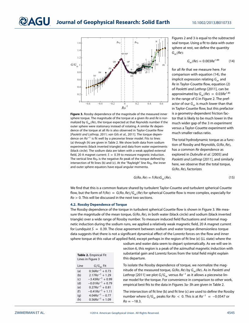
Figure 8. Parameter space map showing magneticReynolds number as a function of inverse Rossby numberfor the four runs of internal magnetic field measurementsin Figure 9. All experiments are run at steady state, butthere is a trend in Rm versus Ro because one sphere orthe other is held at a fixed speed while the speed of theother is varied to change Ro.

The torque as a fraction of the long-term mean isshown on the top, and wall shear stress 𝜏 measuredat a port as a fraction of the long-term mean is shownon the bottom. The lower torque LL state (existingfor 0.2 < Ro−1 < 0.29) is accompanied by a furtherincrease of wall shear stress at the port radius.

The bursty state labeled B exists for 0.067< Ro−1

< 0.2. The transition from the LL to the B state showsanother small drop in G∕G∞ around Ro−1 = 0.2. Thetorque shows peaked bursts toward a higher valuein this state. A time series of torque and wall shearstress at Ro−1 = 0.16 is shown in Figure 7. Again,the torque variations on the inner sphere are corre-lated with lower wall shear stress at the ports on theouter sphere, suggesting that the bursts involve alarge-scale phenomenon.

In the B state a third peak appears in the wall shearstress spectra in Figure 4, and as Ro is increased, even-

tually the higher-frequency peak from the LL state disappears. Throughout the B state, G∕G∞ varies little. Atthe transition from the B to the QP state, G∕G∞ begins to rise.

6. Magnetic Induction, 𝛀 Effect

An important part of understanding the potential for a dynamo in turbulent spherical Couette flow isunderstanding the generation of internal fields. Here we examine the Ω effect by which azimuthal field isgenerated from poloidal field by differential rotation. We do this with weak applied magnetic field in thissection, so that the Lorentz forces are relatively unimportant.

We measure internal azimuthal and cylindrical radial fields, B𝜙 and Bs, using a pair of Hall sensors located60 cm from the axis of rotation and 10 cm outside the inner sphere’s tangent cylinder (through one of theinstrumentation ports in Figure 1e). The sensors are inside the end of a cylindrical stainless steel housingthat is inserted parallel to the rotation axis so that the probe is submerged to a depth 10 cm from the wall ofthe outer sphere.

For several reasons, it was not practical to conduct the experiments in this paper with Rm or Re held con-stant with Ro. We understand the Re dependence of the torque in Figure 3 and data taken at different Recollapse onto one master curve of G∕G∞ versus Ro. We find that the induced field is not quite linear with Rmand do not have a better collapse at this time, so we present a parameter map of the steady state Rm at eachvalue of Ro−1 in Figure 8.

The highest Rm achieved in any experiment here is 715 with strongly counterrotating boundaries. The gen-eration of internal field will be stronger at higher Rm. The induction results in this section do not appear toscale exactly linearly in Rm, suggesting that flow modification from Lorentz force back reaction associatedwith the generation of these fields is already measurable, but this effect is fairly subtle. The internal fieldsin Figure 9 are measured over a large range of Ro with relatively weak applied magnetic field, S = 0.39 (20 Amagnet current).

The fields from the internal probe are made dimensionless by Bs0, the predicted cylindrical radial compo-nent of the applied magnetic field at the location of the probe. As discussed previously, we use a calculatedvalue from the magnet current that has been shown to agree with measurements with no flow so that itis easy to interpret the gain from mean induction. The choice to normalize by the cylindrical radial appliedfield Bs0 is motivated by the assumption that mean azimuthal field generation at this location is caused byrotation-dominated shear flow with strong cylindrical radial dependence and weak axial dependence. If B𝜙

is generated predominately from Bs, then B𝜙∕Bs0 > 1 can be interpreted as Ω effect with gain.

The vertical component of the applied magnetic field, Bz0, at the internal probe’s location is substantiallystronger than the cylindrical component Bs0, with the ratio Bz0∕Bs0 = 4.2. If more of the observed B𝜙 isgenerated from Bz instead of Bs, then the gain due to the Ω effect is weaker but still present.



Figure 9. Mean cylindrical radial (Bs) and mean azimuthal (B𝜙) field 10 cm down from the outer sphere surface at 60 cmcylindrical radius (s = 0.4ro). We plot B𝜙 for Ro > 0 and −B𝜙 for Ro < 0 since its direction reverses as expected with neg-ative differential rotation. Bs0 is the cylindrical radial component of the externally applied field predicted at that location.In these data, the magnet current is 20 A, S = 0.39. Different experimental runs have different Rm, which is the main rea-son that, for example, the black “Run 2" and red “Run 3" curves do not coincide. Scaling by Rm almost collapses these,but not quite, evidence that the hydrodynamic base state is slightly modified by Lorentz force back reaction resultingfrom this internal field generation. However, there is little effect on the torque (Figure 3) or other measurements withthis low applied field value, indicating similarity to the purely hydrodynamic flow.

6.1. Internal Field: Weak Applied FieldFigure 9 shows the internal azimuthal field, B𝜙, and cylindrical radial, Bs, field as a function of Ro−1 at a fixedLundquist number S = 0.39. When Ro < 0, we plot −B𝜙 because, as expected, B𝜙 reverses sign when thedifferential rotation does. It is useful to note here that the applied field has no 𝜙 component, so B𝜙 is entirelysourced by induction, but if there is no poloidal induction, we expect Bs∕Bs0 = 1. There is always measurablegeneration of B𝜙 in Figure 9.

Figure 10. Time series of azimuthal field and torque at Ro−1 = 0.47,Rm = 152, S = 0.59 showing the importance of the hydrodynamic stateon the Ω effect. At constant external driving parameters, the systemundergoes intermittent transitions between the two states as describedin Zimmerman et al. [2011] with very strong Ω effect in the low torqueL state and weak and even occasionally reversed Ω effect in the hightorque H state.

For comparison between Figures 9 and3 we have also plotted the Rossby num-ber of the Ro < 0 peak in G∕G∞ (RoP)and of the Rayleigh line, (RoR). The peakazimuthal field generation happens atabout Ro = 6 or Ro−1 = 0.167 andshows large gain, up to a factor of 7.5at S = 0.39, and a bit higher at lowerS. The large jump around Ro−1 = 0.5 isthe H-L transition. This is consistent withthe picture in Zimmerman et al. [2011]of the emergence of a fast zonal flowwith a sharp shear in the L state with aboundary near the tangent cylinder. Themeasurements in Figure 9 are taken at1.2 times the tangent cylinder radius, andthe strong Ω effect implies strong shearin the azimuthal velocity here.

In Figure 10 we show some transitionsbetween high and low torque states atfixed Rossby Ro−1 = 0.47 with S = 0.59and Rm = 152.



0.5 1.5 2.5 3.5 4 4.50 1 2 3

S

0.9

1

1.1

1.2

1.3

1.4

0

2

4

6

8

10B

Bs

Figure 11. Azimuthal and cylindrical radial induced field atRo = 6 (Bursty B hydrodynamic state) and Rm = 477 withvarying Lundquist number S. B𝜙 (black circle) as a fractionof the applied field at the probe location is sharplyreduced with increasing S, while Bs (black inverted triangle)grows appreciably.

At higher positive Ro than the H-L state transition,the Ω effect intensifies with increasing positiveRo up until the peak which is near the onset ofthe B state. The transition from the B to the QPstate is accompanied by a drop in the Ω effectand a substantial increase in the mean poloidalinduction. This induction is opposing the appliedfield, weakening and even reversing Bs.

The generation of B𝜙 at the probe location isgreatly reduced near the negative Rossby peak inG∕G∞ (RoP in Figures 3 and 9), though the min-imum Ω effect is slightly offset from the torquemaximum. An interesting feature right at theG∕G∞ peak is strong poloidal induction aiding Bs,increasing it to more than twice the applied value.

This is reminiscent of the sharp peak of induced poloidal magnetic field reported by Nataf et al. [2008] in theDTS experiment. In that experiment, it was interpreted as a consequence of a stronger poloidal fluid flow asthe geostrophic constraints due to rotation vanish.

There is substantial Ω effect for Ro < 0 as well, with a maximum value of B𝜙∕Bs0 = 3.2 at Ro = −2.75,Ro−1 = −0.36. Note, however, from Figure 8 that the magnetic Reynolds number here is about half that atthe Ro = 6 peak and changes substantially with Ro−1 since in Run 4 we were keeping the outer sphere speedconstant and changing ΔΩ. In fact, for Ro−1 < −0.4 the Ω effect scaled by Rm is about constant and aboutthe same as that at the positive Rossby peak. We do expect strong shear near the tangent cylinder in thisrange, as in the simulations at Ro−1 = −1.67 by Matsui et al. [2011].

Predicting supercritical dynamo action in high Reynolds number spherical Couette flow requires the abilityto capture the complex Rossby dependence of the flows and fields. Many of the Rossby-dependent featuresmeasured here have not been predicted or reported in spherical Couette simulations carried out at lower Re.

Some care should be taken with the Ω effect interpretation of Figure 9 since the measurements are takenat a single point. The strengthening and weakening of the azimuthal field in Figure 9 could reflect changesin the position of strong Ω effect toward or away from our measurement location rather than an increaseor decrease in production of azimuthal field from poloidal field. Unfortunately, we cannot at this time moveour probe significantly in cylindrical radius to test this idea. Still, the measurements of Figure 9 should beuseful to compare against a similar point measurement taken from a simulation.

7. High Applied Field: 𝛀 Effect Reduction and Dynamo-Like Bursts

The results in the preceding sections were in weak field regimes where the Lorentz force has little effecton the fluid flow. However, as the external magnetic field is increased, we access different states at givenhydrodynamic parameters.

In this section we will describe results of increasing the applied field at Ro = 6, E = 1.2 × 10−7, andRm = 477. This initial state is at the peak of the Ω effect for small Lundquist number in section 6.

7.1. Mean Internal Field: Strong FieldFigure 11 shows internal azimuthal and radial field induction (normalized by Bs0) as a function of Lundquistnumber. We may interpret B𝜙∕Bs0 in Figure 11 as a reduction of the Ω effect due to growing Lorentz forces inthe flow as the power required to produce the observed toroidal field substantially reduces the shear in thefluid. This is similar to a reduction of the Ω effect observed by Verhille et al. [2012].

Though B𝜙∕Bs0 monotonically decreases throughout Figure 11, the strength of the azimuthal field B𝜙

increases up to S = 2.75, reaching a peak strength of 40 G. Above the kink in B𝜙∕Bs0 at S = 2.75, B𝜙 dropsand reaches a low of 17 G at the strongest applied field, S = 4.2.

As S is increased above 0.5, Bs∕Bs0 grows. This internal poloidal field growth is most likely concurrent withthe observed increase of the mean external dipole moment described later, a phenomenon we believe



Figure 12. RMS fluctuations of Bml

= l(l + 1)gml

for selected sphericalharmonic contributions (top) normalized by the reference field B0, andthe torque on the inner sphere G (bottom) normalized by the torqueat S = 0, G0.

happens through a dynamo-stylefeedback loop involving bothaxisymmetric and nonaxisymmetricflow components.

7.2. Bursting State OnsetThe drop in B𝜙∕Bs0 as S is increasedabove 2.75 is shortly followed by theonset of a new flow state with muchstronger fluctuations in several Gausscoefficients, significantly higher torqueon the inner sphere, and bursts ofthe axial dipole Gauss coefficientg0

1 in a direction that augments theapplied field.

The onset of this dipole-bursting stateis shown in Figure 12, which shows theRMS level of fluctuations (Bm

l = l(l+1)gml )

of each Gauss coefficient (or of a nonaxisymmetric pair representing an azimuthally drifting pattern). AboveS = 3.1, there is a substantial increase in the strength of the nonaxisymmetric components B1

2, B23, and B3

4,an increase in the fluctuations of B0

1 and B03, and an increase in the mean of B0

1. Time series of these externalfield components at S = 3.5 are shown in Figure 13.

The torque on the inner sphere is also shown in Figure 12, normalized by its purely hydrodynamic value atzero applied field. The torque increases with S but begins to increase most rapidly around S = 2.75 where B𝜙

peaks, just before the growth of the strong fluctuations in the new state.

7.3. Mode Interactions: Time EvolutionIn Figure 13 we show the time evolution of the state at S = 3.5, Ro = 6, E = 1.2 × 10−7, and Rm = 477.The quantity on top is Psym = P1∕𝜎P1

+ P3∕𝜎P3where P1 and P3 are the signals from two pressure sensors in

Figure 13. Time series at S = 3.5, near onset of the new dynamical state at strong S in Figure 12. Bml= l(l+1)gm

l. In order

from top, Psym, sum of pressure signals from instrumentation port sensors located 180◦ apart, B0l

, axisymmetric m = 1and m = 3 magnetic field components, the most active nonaxisymmetric field components B1

2, B23, and B3

4, and at thebottom, torque on the inner sphere normalized by the torque at Ro = 6, S = 0. These dynamics suggest dynamo-stylefeedback that enhances the applied field, as we discuss in the text.



(a) (b)

Figure 14. Two different interaction diagrams of externally mea-sured magnetic field components Sm

land internal field compo-

nents T ml

with underlying poloidal and toroidal velocity modessm

land tm

lare supported by our data. Directly observed exter-

nal field components are in circles and colored as in Figure 12.We do not have spatial information about the internal toroidalfields, shown here in blue boxes. In scenario (a) the S1

2 is inducedfrom the axial dipole by a poloidal velocity field s1

1. Instead,in (b) S1

2 arises from the other two nonaxisymmetric modes,perhaps then causing a back reaction reducing the s2

2 and s33

velocity fields.

ports 180◦ apart, normalized by theirstandard deviations 𝜎Pn

to remove slightdifferences in calibration. This combina-tion emphasizes large-scale fluctuationswith even azimuthal wave number m.

We plot five induced field components, theaxisymmetric dipole B0

1 and axisymmetricl = 3 component B0

3. The contribution tothese components from the applied fieldhave been subtracted and positive val-ues of B0

1 correspond to an increase in thedipole that augments the applied field.The mean value of the dipole field B0

1 aver-aged over many bursts is 5% above theapplied value by S = 4.2. As discussedin section 2.3, the applied B0

3 is oppo-site in sign to the applied B0

1, and so thepositive-going B0

3 bursts in Figure 13 arereductions in the total B0

3 field.

We also plot nonaxisymmetric compo-nents B1

2, B23, and B3

4. The five poloidalcomponents in Figure 13 dominate thefluctuations seen in the external measuredfield at these parameters. The nonaxisym-metric components rotate in a progradedirection with similar phase speeds,𝜔∕(mΩo) = 0.4.

The growth of the nonaxisymmetric components B23 and B3

4 is clearly correlated with the growth of theaxisymmetric components, and both are accompanied by increase in the torque on the inner sphere, shownat the bottom and normalized by its hydrodynamic value when S = 0. To guide the eye, lines (a) and (b) inFigure 13 are at a maximum and a minimum of the torque as a function of time.

The fluctuations in this section bear a resemblance to the behavior seen in the high torque state and thehigh-to-low transitions discussed in section 5. The high torque state at lower Ro and weak applied magneticfield discussed in section 5.5 also shows similar bursts of B1

2, B23, and B3

4 synchronized with mean and fluctu-ating enhancements of the dipole. Many of the details of the temporal dynamics are different, though. Thetrio of nonaxisymmetric components drift half as fast at Ro ≃ 2 than Ro = 6. The weakly magnetized hightorque state also shows mean and fluctuating dipole enhancement synchronized with the growth of thenonaxisymmetric modes.

7.4. A Possible Dynamo-Style FeedbackThe coupling between the nonaxisymmetric components and the axisymmetric components in Figure 13is notable. Using the selection rules for flow and field from Bullard and Gellman [1954], we can put forthtwo conjectures on the nature of the dipole-reinforcing bursts. Here we will use sm

l and tml for poloidal and

toroidal velocity components and Sml and T m

l for poloidal and toroidal magnetic field components. There canbe no toroidal field in the current-free region external to the sphere, so all of the components we directlyobserve are external poloidal fields Sm

l . We note that whenever a magnetic field is induced by a velocityfield, energy and momentum conservation require a Lorentz force effect on the velocity field. The enhancedtorque in this state is also evidence of significant Lorentz forces.

We assume underlying nonaxisymmetric flow components with m = 1, m = 2, and m = 3. Psym in Figure 13is direct evidence for a m = 2 flow component synchronized with the S2

3 external induction.

Our imposed differential rotation is expected to be dominated by the axisymmetric component t01. This t0

1flow could lead to substantial gain in magnetic field, though that gain is reduced from the hydrodynamicbase state as per Figure 11.



Each burst of B01 and B0

3 in Figure 13 is synchronized with the growth of the nonaxisymmetric componentsB2

3 and B34. Spence et al. [2006] were the first to report on the induction of an axisymmetric dipole in the

Madison dynamo experiment. They demonstrate that an axial dipole moment measured external to thecurrent-carrying region cannot be induced directly from an axisymmetric applied field by an axisymmet-ric flow. Spence et al. [2006] explain their external axial dipole induction as the net contribution of thenonaxisymmetric turbulent fluctuations.

We note that the induced dipole adds to the imposed field in our case, while in the Madison experiment itwas always opposite, reducing the total dipole.

We show several possibilities of allowed interactions in Figure 14a, assuming that the internal nonaxisym-metric components are the poloidal flows s1

1, s22, and s3

3. There is a one-step coupling by which those velocityfields can induce the observed nonaxisymmetric fields from the applied axisymmetric field. We do not drawan exhaustive network diagram in Figure 14a, as there are 41 allowed interactions involving just the eightfield components and four flow components shown there, just to list a few simple possibilities that areconsistent with the behavior in Figure 13.

There are three conceptually similar triads (e.g., S01, S2

3, and T 22 ) where an underlying sl

l velocity componentinduces the externally observed poloidal component Sl

l+1 from S01 and S0

3. That poloidal component is con-verted to an internal toroidal T l

l by the action of the differential rotation t01, and the T l

l toroidal componentcan be converted to S0

1 and S03 by the sl

l poloidal velocity field. Note that each triad has a possible dynamomechanism similar to that discussed in Bullard and Gellman [1954].

We present another similar interaction diagram in Figure 14b, this time inducing the S12 component from

either of the large S23 or S3

4 fields. Note that in Figure 13 S12 arises slightly later than either S2

3 or S34. Also evi-

dent is that as S12 grows, the enhanced dipole S0

1 and modes S23 and S3

4 fall, possible evidence for a strongLorentz force back reaction caused by the production of S1

2. Again, we do not show the large number of totalpossible connections.

Assuming some radial dependence for the internal flow and field components and constructing a reducedinduction equation model could be fruitful, as it would allow us to know which interactions were strongest,but this is beyond the scope of this paper. Nevertheless, these are more results that could provide a goodbenchmark for geodynamo codes.

As we do not have conclusive evidence supporting either scenario in Figure 14, we have included bothfor scientific completeness. We expect future research can distinguish between them. A complete under-standing of the scenarios set out in Figure 14 may be of particular geophysical relevance. The observationshere are consistent with differential rotation generating toroidal field plus a few nonaxisymmetric driftingcomponents that may be similar to Rossby waves. In this sense, they would be similar to the cartridge beltdynamo scenario seen in the onset of rotating convection in a spherical shell.

The fact that we seem to have large-scale poloidal motions closing an axial-dipole-enhancing induction loopis encouraging. It points to the possibility of understanding these dynamics with reduced models of the flowand untangling how the small-scale turbulence interacts with the large-scale motions in both magnetizedand unmagnetized states.

8. Summary and Conclusions

We present a number of novel experimental results in hydrodynamic and hydromagnetic spherical Couetteexperiments at unprecedented magnetic and hydrodynamic Reynolds number. We look at angular momen-tum transport without appreciable magnetic field effects and find broad similarity with recent results fromTaylor-Couette flow over part of the accessible range of Rossby number but find dramatic restructuring ofthe flow and strong enhancement of angular momentum transport, possibly involving large-scale Rossbywaves, when 1 < Ro < 5. Changing Re alone while holding Ro fixed leads to expected turbulent flowscalings. The similarities and differences in the Ro dependence of turbulent angular momentum transportbetween spherical and Taylor Couette flow may have interesting implications for understanding angularmomentum transport in rotating geophysical systems.

The Ro dependence of the hydrodynamic mean flow confers a strong Rossby dependence on the Ω effect,the generation of internal azimuthal magnetic field from poloidal field. Although we do not observe a



self-excited magnetic dynamo in the current set of experiments up to half speed, we do observe substantialgain in the poloidal-to-toroidal field conversion over a large range of Ro.

Applying a strong magnetic field at Ro = 6, the peak of low-field azimuthal field generation, reduces theΩ effect, a phenomenon that may be important for saturation of geophysical and astrophysical dynamos.Strong enough field leads to the onset of a different dynamical state with higher torque and bursts of non-axisymmetric magnetic field and velocity fluctuations that are correlated with bursts in enhancement ofaxisymmetric external fields. The nonaxisymmetric fluctuations, like those in the high torque hydrodynamicstate, seem to be a trio of drifting waves that may be Rossby waves.

The dipole bursts are plausibly generated by a dynamo-style feedback loop that involves differential rota-tion and drifting waves, a scenario that is of substantial geophysical and astrophysical interest. We are just atthe beginning of hydromagnetic experiments in this facility, but these early results suggest a rich interplayof turbulence, rotation, and magnetic fields, as in a planet’s liquid metal core.

ReferencesBerhanu, M., et al. (2007), Magnetic field reversals in an experimental turbulent dynamo, Europhys. Lett., 77 (5), 59,001,

doi:10.1209/0295-5075/77/59001.Berhanu, M., et al. (2010), Dynamo regimes and transitions in the VKS experiment, Eur. Phys. J. B, 77 (4), 459–468,

doi:10.1140/epjb/e2010-00272-5.Brauckmann, H. J., and B. Eckhardt (2013), Intermittent boundary layers and torque maxima in Taylor-Couette flow, Phys. Rev. E, 87,

033004, doi:10.1103/PhysRevE.87.033004.Brito, D., T. Alboussière, P. Cardin, N. Gagnière, D. Jault, P. La Rizza, J.-P. Masson, H.-C. Nataf, and D. Schmitt (2011), Zonal shear and

super-rotation in a magnetized spherical Couette-flow experiment, Phys. Rev. E, 83(6), 066310, doi:10.1103/PhysRevE.83.066310.Bullard, E., and H. Gellman (1954), Homogeneous dynamos and terrestrial magnetism, Philos. Trans. R. Soc. London, Ser. A, 247(928),

213–278.Busse, F. H. (1970), Thermal instabilities in rapidly rotating systems, J. Fluid Mech., 44(3), 441–460.Cardin, P., D. Brito, D. Jault, H.-C. Nataf, and J.-P. Masson (2002), Towards a rapidly rotating liquid sodium dynamo experiment,

Magnetohydrodynamics, 38(1), 177–189.Dubrulle, B., O. Dauchot, F. Daviaud, P.-Y. Longaretti, D. Richard, and J.-P. Zahn (2005), Stability and turbulent transport in Taylor–Couette

flow from analysis of experimental data, Phys. Fluids, 17(9), 095103, doi:10.1063/1.2008999.Fink, J., and L. Leibowitz (1995), Thermodynamic and transport properties of sodium liquid and vapor, Tech. Rep. ANL/RE–95/2, Argonne

National Laboratory.Frick, P., V. Noskov, S. Denisov, and R. Stepanov (2010), Direct measurement of effective magnetic diffusivity in turbulent flow of liquid

sodium, Phys. Rev. Lett., 105(18), 184502, doi:10.1103/PhysRevLett.105.184502.Gailitis, A., O. Lielausis, E. Platacis, S. Dement’ev, A. Cifersons, G. Gerbeth, T. Gundrum, F. Stefani, M. Christen, and G. Will (2001), Magnetic

field saturation in the Riga dynamo experiment, Phys. Rev. Lett., 86, 3024–3027, doi:10.1103/PhysRevLett.86.3024.Gailitis, A., G. Gerbeth, T. Gundrum, O. Lielausis, E. Platacis, and F. Stefani (2008), History and results of the Riga dynamo experiments, C.R.

Phys., 9(7), 721–728, doi:10.1016/j.crhy.2008.07.004.Gillet, N., D. Jault, E. Canet, and A. Fournier (2010), Fast torsional waves and strong magnetic field within the Earth’s core, Nature,

465(7294), 74–77, doi:10.1038/nature09010.Gillet, N., N. Schaeffer, and D. Jault (2011), Rationale and geophysical evidence for quasi-geostrophic rapid dynamics within the Earth’s

outer core, Phys. Earth Planet. Inter., 187(3–4), 380–390, doi:10.1016/j.pepi.2012.03.006.Holme, R. (2007), Large-scale flow in the core, in Treatise on Geophysics, vol. 8, Core Dynamics, edited by P. Olson and G. Schubert,

pp. 107–129, Elsevier B. V., Amsterdam.Huisman, S. G., D. P. M. van Gils, S. Grossmann, C. Sun, and D. Lohse (2012), Ultimate turbulent Taylor-Couette flow, Phys. Rev. Lett.,

108(024,501), doi:10.1103/PhysRevLett.108.024501.Jackson, D. (1975), Classical Electrodynamics, John Wiley, New York.Jault, D. (2008), Axial invariance of rapidly varying diffusionless motions in the Earth’s core interior, Phys. Earth Planet. Inter., 166, 67–76.Kelley, D. H., S. A. Triana, D. S. Zimmerman, A. Tilgner, and D. P. Lathrop (2007), Inertial waves driven by differential rotation in a planetary

geometry, Geophys. Astrophys. Fluid Dyn., 101(5–6), 469–487, doi:10.1080/03091920701561907.Kelley, D. H., S. A. Triana, D. S. Zimmerman, and D. P. Lathrop (2010), Selection of inertial modes in spherical Couette flow, Phys. Rev. E,

81(2), 026311, doi:10.1103/PhysRevE.81.026311.Lathrop, D., W. Shew, and D. Sisan (2001), Laboratory experiments on the transition to MHD dynamos, Plasma Phys. Controlled Fusion,

43(12A), A151–A160, doi:10.1088/0741-3335/43/12A/311, 28th EPS Conference on Controlled Fusion and Plasma Physics, FUNCHAL,PORTUGAL, JUN 18-22, 2001.

Lemmon, E., M. McLinden, and D. Friend (2013), NIST Chemistry WebBook. NIST Standard Reference Database Number 69, chap.,Thermophysical Properties of Fluid Systems, National Institute of Standards and Technology, Gaithersburg, Md.

Matsui, H., M. Adams, D. Kelley, S. Triana, D. Zimmerman, B. Buffet, and D. Lathrop (2011), Numerical and experimental investigation ofshear-driven inertial oscillations in an Earth-like geometry, Phys. Earth Planet. Inter., 188, 194–202, doi:10.1016/j.pepi.2011.07.012.

Monchaux, R., et al. (2007), Generation of a magnetic field by dynamo action in a turbulent flow of liquid sodium, Phys. Rev. Lett., 98(4),044502, doi:10.1103/PhysRevLett.98.044502.

Monchaux, R., et al. (2009), The von Kármán Sodium experiment: Turbulent dynamical dynamos, Phys. Fluids, 21(3), 035108,doi:10.1063/1.3085724.

Nataf, H.-C. (2013), Magnetic induction maps in a magnetized spherical Couette flow experiment, C.R. Phys., 14(2–3), 248–267,doi:10.1016/j.crhy.2012.12.002.

Nataf, H.-C., and N. Gagnière (2008), On the peculiar nature of turbulence in planetary dynamos, C.R. Phys., 9(7), 702–710,doi:10.1016/j.crhy.2008.07.009.

AcknowledgmentsWe gratefully acknowledge grantsupport from NSF Earth Sciences.Design and construction of this majorresearch facility were supported byNSF/MRI EAR-0116129, and continu-ing scientific work is supported by NSFEAR-1114303. We thank Don Martinand Nolan Ballew at UMD for invalu-able technical support and SimonCabanes from UJF Grenoble for helpwith the Hall sensor array design andinstallation, and Matthew Adams atUMD for help with experimental runs.The stay of H.C.N. at UMD was madepossible, thanks to support by UMD,CNRS, and University of Grenobleunder Memorandun of UnderstandingCNRS-723684/00.


http://dx.doi.org/10.1209/0295-5075/77/59001

http://dx.doi.org/10.1140/epjb/e2010-00272-5

http://dx.doi.org/10.1103/PhysRevE.87.033004


http://dx.doi.org/10.1063/1.2008999

http://dx.doi.org/10.1103/PhysRevLett.105.184502


http://dx.doi.org/10.1016/j.crhy.2008.07.004

http://dx.doi.org/10.1038/nature09010

http://dx.doi.org/10.1016/j.pepi.2012.03.006


http://dx.doi.org/10.1080/03091920701561907


http://dx.doi.org/10.1088/0741-3335/43/12A/311



http://dx.doi.org/10.1063/1.3085724




Nataf, H.-C., T. Alboussière, D. Brito, P. Cardin, N. Gagnière, D. Jault, and D. Schmitt (2008), Rapidly rotating spherical Couetteflow in a dipolar magnetic field: An experimental study of the mean axisymmetric flow, Phys. Earth Planet. Inter., 170, 60–72,doi:10.1016/j.pepi.2008.07.034.

Ostilla, R., R. J. A. M. Stevens, S. Grossmann, R. Verzicco, and D. Lohse (2013), Optimal Taylor Couette flow: Direct numerical simulations,J. Fluid Mech, 719, 14–46, doi:10.1017/jfm.2012.596.

Paoletti, M. S., and D. P. Lathrop (2011), Angular momentum transport in turbulent flow between independently rotating cylinders, Phys.Rev. Lett., 106(2), 024501, doi:10.1103/PhysRevLett.106.024501.

Paoletti, M. S., D. P. M. van Gils, B. Dubrulle, C. Sun, D. Lohse, and D. P. Lathrop (2012), Angular momentum transport and turbulence inlaboratory models of Keplerian flows, A&A, 547, A64, doi:10.1051/0004-6361/201118511.

Petrelis, F., M. Bourgoin, L. Marie, J. Burguete, A. Chiffaudel, F. Daviaud, S. Fauve, P. Odier, and J. Pinton (2003), Nonlinear magneticinduction by helical motion in a liquid sodium turbulent flow, Phys. Rev. Lett., 90(17), 174501, doi:10.1103/PhysRevLett.90.174501.

Rahbarnia, K., et al. (2012), Direct observation of the turbulent EMF and transport of magnetic field in a liquid sodium experiment,Astrophys. J., 759(2), 80.

Ravelet, F., R. Delfos, and J. Westerweel (2010), Influence of global rotation and reynolds number on the large-scale features of aturbulent Taylor-Couette flow, Phys. Fluids, 22(5), 055103, doi:10.1063/1.3392773.

Rieutord, M., S. Triana, D. Zimmerman, and D. Lathrop (2012), Excitation of inertial modes in an experimental spherical Couette flow,Phys. Rev. E, 86, 026304, doi:10.1103/PhysRevE.86.026304.

Sisan, D. R. (2004), Hydromagnetic turbulent instability in liquid sodium experiments, PhD thesis, University of Maryland,College Park, Md.

Spence, E. J., M. D. Nornberg, C. M. Jacobson, R. D. Kendrick, and C. B. Forest (2006), Observation of a turbulence-induced large scalemagnetic field, Phys. Rev. Lett., 96, 055002, doi:10.1103/PhysRevLett.96.055002.

Stieglitz, R., and U. Müller (2001), Experimental demonstration of a homogeneous two-scale dynamo, Phys. Fluids, 13, 561–564,doi:10.1063/1.1331315.

van Gils, D. P. M., S. G. Huisman, G.-W. Bruggert, C. Sun, and D. Lohse (2011), Torque scaling in turbulent Taylor-Couette flow with co- andcounterrotating cylinders, Phys. Rev. Lett., 106(2), 024502, doi:10.1103/PhysRevLett.106.024502.

van Gils, D. P. M., S. G. Huisman, S. Grossmann, C. Sun, and D. Lohse (2012), Optimal Taylor-Couette turbulence, J. Fluid Mech., 706,118–149, doi:10.1017/jfm.2012.236.

Verhille, G., R. Khalilov, N. Plihon, P. Frick, and J.-F. Pinton (2012), Transition from hydrodynamic turbulence to magnetohydrodynamicturbulence in von Kármán flows, J. Fluid Mech., 693, 243–260, doi:10.1017/jfm.2011.522.

Wicht, J. (2014), Flow instabilities in the wide-gap spherical couette system, J. Fluid Mech., 738, 184–221, doi:10.1017/jfm.2013.545.Zhang, K., P. Earnshaw, X. Liao, and F. H. Busse (2001), On inertial waves in a rotating fluid sphere, J. Fluid Mech., 437, 103–119,

doi:10.1017/S0022112001004049.Zimmerman, D. S. (2010), Turbulent shear flow in a rapidly rotating spherical annulus, PhD thesis, University of Maryland,

College Park, Md.Zimmerman, D. S., S. A. Triana, and D. P. Lathrop (2011), Bi-stability in turbulent, rotating spherical Couette flow, Phys. Fluids, 23(6),

065104, doi:10.1063/1.3593465.



http://dx.doi.org/10.1017/jfm.2012.596


http://dx.doi.org/10.1051/0004-6361/201118511


http://dx.doi.org/10.1063/1.3392773



http://dx.doi.org/10.1063/1.1331315





http://dx.doi.org/10.1017/S0022112001004049

http://dx.doi.org/10.1063/1.3593465

Documents

A turbulent, high magnetic Reynolds number experimental model of Earth's core