A Three-StageMathematical-Programming Methodfor the Multi-Floor Facility Layout

Problem

by

Sabrina Bernardi

A research paperpresented to the University of Waterloo

in partial fulfillment of the requirements for the degree ofMaster of Mathematics

inComputational Mathematics

Supervisor: Dr. Miguel Anjos

Waterloo, Ontario, Canada, 2010

c© Sabrina Bernardi 2010

I hereby declare that I am the sole author of this report. This is a true copy of the report,including any required final revisions, as accepted by my examiners.

I understand that my report may be made electronically available to the public.

ii

Abstract

The purpose of this research paper is to present a three-stage method using mathematical-programming techniques that finds high-quality solutions to the multi-floor facility layoutproblem. The first stage is a linear mixed-integer program that assigns departments tofloors such that the total of the departmental interaction costs between floors is globallyminimized. Subsequent stages find a locally optimal layout for each floor. Two versionsof the proposed approach are considered. The first solves the layout of each floor inde-pendently of the other floors, allowing up to one elevator location. The second solves thelayout of all floors simultaneously, allowing for multiple elevator locations. Variations tothe problem and to the basic method are also investigated. The two versions are tested andcompared to each other through computational experiments and also to existing results inthe literature. It is clear that the proposed method can provide several high-quality layoutsfor medium and large-scale problem instances. Not only does it achieve competitive resultscompared to previous methods, but it also overcomes some of their limitations.

iii

Contents

List of Tables viii

List of Figures ix

1 Introduction 1

2 Literature Review 3

2.1 Single-Stage Approaches . . . . . . . . . . . . . . . . . . . . . . . . . . . . 3

2.1.1 Exchange-Based Heuristics . . . . . . . . . . . . . . . . . . . . . . . 3

2.1.2 Simulated-Annealing Based Algorithms . . . . . . . . . . . . . . . . 5

2.1.3 Genetic-Based Algorithms . . . . . . . . . . . . . . . . . . . . . . . 6

2.1.4 Mathematical Programming Techniques . . . . . . . . . . . . . . . 8

2.2 Multi-Stage Approaches Combining Exact and Heuristic Procedures . . . . 10

3 Background for New Mathematical Programming Approach 15

3.1 Dispersion Concentration Method (DISCON) . . . . . . . . . . . . . . . . 15

3.2 Nonlinear Optimization Layout Technique (NLT) . . . . . . . . . . . . . . 16

3.3 The Anjos-Vannelli Facility-Layout Design . . . . . . . . . . . . . . . . . . 17

3.3.1 Stage One: ModCoAR . . . . . . . . . . . . . . . . . . . . . . . . . 18

3.3.2 Stage Two: BPL . . . . . . . . . . . . . . . . . . . . . . . . . . . . 22

3.3.3 Aspect-Ratio Constraints . . . . . . . . . . . . . . . . . . . . . . . . 23

iv

4 Three-Stage Multi-Floor Facility Layout Method 24

4.0.4 Solving Each Floor Independently vs. All Floors Simultaneously . . 25

4.1 Notation for the Three-Stage Multi-Floor Model . . . . . . . . . . . . . . . 25

4.2 Stage One: Assigning Departments to Floors . . . . . . . . . . . . . . . . . 26

4.3 Stages Two and Three: Optimizing the Layout of Each Floor . . . . . . . . 27

4.3.1 FBF: Optimizing the Layout of Each Floor Independently . . . . . 28

4.3.2 AFS: Optimizing the Layout of Each Floor Simultaneously . . . . . 32

5 Computational Experiments 37

5.1 Choosing Parameters . . . . . . . . . . . . . . . . . . . . . . . . . . . . . . 37

5.1.1 Investigating The Choice of Parameters KMOD and α . . . . . . . . 39

5.2 Slack Space . . . . . . . . . . . . . . . . . . . . . . . . . . . . . . . . . . . 40

5.3 Case of a Narrow Facility . . . . . . . . . . . . . . . . . . . . . . . . . . . . 41

5.4 Test Problem 1: 15-Departments and 3-Floors . . . . . . . . . . . . . . . . 42

5.4.1 Application of FBF to Test Problem 1 . . . . . . . . . . . . . . . . 43

5.4.2 Application of AFS to Test Problem 1 . . . . . . . . . . . . . . . . 44

5.4.3 Application of AFS to Test Problem 1- AFS-C vs. AFS-NC . . . . 45

5.4.4 Comparing Proposed Methods to MFFLPE . . . . . . . . . . . . . 46

5.4.5 Comparison of Results for Test Problem 1 . . . . . . . . . . . . . . 48

5.5 Test Problem 2: 40-Departments and 4-Floors . . . . . . . . . . . . . . . . 49

5.5.1 Application of FBF to Test Problem 2 . . . . . . . . . . . . . . . . 50

5.5.2 Application of AFS to Test Problem 2- AFS-C vs. AFS-NC . . . . 51

5.5.3 Comparison of Results for Test Problem 2 . . . . . . . . . . . . . . 51

5.6 Summary of Computational Experiments . . . . . . . . . . . . . . . . . . . 52

6 Conclusions and Future Research 53

APPENDICES 55

v

A Test Data for Computational Experiments 56

A.1 Data for the Armour and Buffa 20-Department Problem . . . . . . . . . . 56

A.2 Data for 15-Department and 3-Floor Problem . . . . . . . . . . . . . . . . 58

A.3 Data for 40-Department and 4-Floor Problem . . . . . . . . . . . . . . . . 60

References 64

vi

List of Tables

2.1 Department Areas . . . . . . . . . . . . . . . . . . . . . . . . . . . . . . . 4

5.1 Parameters and Costs for Figure 5.1 . . . . . . . . . . . . . . . . . . . . . . 38

5.2 Generalized Target Distances vs. Total Costs: Armour and Buffa 20-DepartmentProblem . . . . . . . . . . . . . . . . . . . . . . . . . . . . . . . . . . . . . 40

5.3 Investigating Slack Space on Quality of Solution (no aspect ratio constraints) 41

5.4 Investigating Slack Space on Quality of Solution (aspect ratio constraints of3.0) . . . . . . . . . . . . . . . . . . . . . . . . . . . . . . . . . . . . . . . . 41

5.5 Results of FBF on Test Problem 1 . . . . . . . . . . . . . . . . . . . . . . . 44

5.6 Results of AFS on Test Problem 1 . . . . . . . . . . . . . . . . . . . . . . . 45

5.7 AFS-C vs. AFS-NC . . . . . . . . . . . . . . . . . . . . . . . . . . . . . . . 46

5.8 Results: AFS-C . . . . . . . . . . . . . . . . . . . . . . . . . . . . . . . . 46

5.9 Results: AFS-NC . . . . . . . . . . . . . . . . . . . . . . . . . . . . . . . . 46

5.10 Fixed Area of Departments . . . . . . . . . . . . . . . . . . . . . . . . . . 47

5.11 Results: AFS-C . . . . . . . . . . . . . . . . . . . . . . . . . . . . . . . . . 51

5.12 Results: AFS-NC . . . . . . . . . . . . . . . . . . . . . . . . . . . . . . . . 51

A.1 Initial Configuration for Armour and Buffa 20-Department Problem . . . . 56

A.2 Costs for Armour and Buffa 20-Department Problem . . . . . . . . . . . . 57

A.3 Fixed Area of Departments for Armour and Buffa 20-Department Problem 57

A.4 Vertical Cost for 15-Department and 3-Floor Problem . . . . . . . . . . . . 58

A.5 Flow Matrix for 15-Department and 3-Floor Problem . . . . . . . . . . . . 59

A.6 Horizontal Costs for 15-Department and 3-Floor Problem . . . . . . . . . . 59

vii

A.7 Fixed Area of Departments for 15-Department and 3-Floor Problem . . . . 60

A.8 Flow Data for 40-Department and 4-Floor Problem . . . . . . . . . . . . . 60

A.9 Initial Configuration for 40-Department and 4-Floor Problem . . . . . . . . 61

A.10 Fixed Area of Departments for 40-Department and 4-Floor Problem . . . . 61

viii

List of Figures

3.1 The theoretical concept of target distances. . . . . . . . . . . . . . . . . . . 19

3.2 Final layouts of Armour and Buffa 20-department problem using Anjos-Vannelli Method [3]. . . . . . . . . . . . . . . . . . . . . . . . . . . . . . . 23

5.1 Solutions to ModCoAR for the Armour and Buffa 20-department problem. 38

5.2 Results of ModCoAR and BPL for the lowest cost solution found. . . . . . 39

5.3 Infeasible solution of Multi-ModCoAR before scaling radii. . . . . . . . . . 42

5.4 Solution of Multi-ModCoAR after radii is scaled by 0.8. . . . . . . . . . . . 42

5.5 Final layout obtained by MULTIPLE. The figure comes from [5]. . . . . . 43

5.6 Final layout obtained by FBF. . . . . . . . . . . . . . . . . . . . . . . . . . 44

5.7 Final Layout using AFS with a cost of 125,104.35. . . . . . . . . . . . . . . 45

5.8 The optimal floor layout obtained by Goetschalckx et al. [10]. The figurewas taken from [10]. . . . . . . . . . . . . . . . . . . . . . . . . . . . . . . 47

5.9 The final layout obtained from FBF. . . . . . . . . . . . . . . . . . . . . . 47

5.10 The spacefilling curve and fixed department locations for the 40-departmentand 4-floor problem. Figure comes from [21]. . . . . . . . . . . . . . . . . 49

5.11 Layout obtained using FBF. . . . . . . . . . . . . . . . . . . . . . . . . . . 50

ix

Chapter 1

Introduction

In general, facility layout problems involve finding the optimal arrangement of departmentswithin a facility. Interaction costs between departments of given areas are minimized inthe optimal arrangement. Many applications of this general problem exist and include ar-ranging departments in production facilities, in hotels, in office buildings, and in hospitals,to name a few. There are several variations to the problem, all of which are NP-hard [3].Even the quadratic assignment problem, which is the special case of assigning N depart-ments to N fixed locations with departments of fixed, equal shapes is NP-hard [12].

A particular case of the general facility layout problem is the multi-floor facility layoutproblem which, as the name suggests, involves finding the optimal arrangement of depart-ments in a facility having multiple floors. More constraints arise in the multi-floor problemin addition to those already present in the single floor case; this adds to the complexityof the problem. Not only must the interaction between departments on the same floor beconsidered, but also the interaction between departments that are on different floors of thefacility. This requires the use and placement of elevators and/or stairwells to facilitate themovement of material between floors. Due to the complexity of the problem, many multi-floor approaches have several limitations. These may include the inability to accommodatemultiple elevator locations, the need to split departments across floors, and computationaltimes that are too high for practical use.

In general, the objective function for the multi-floor facility layout problem can be givenas

min∑i

∑j

(cHijdHij + cVijd

Vij)fij,

where fij is a parameter denoting the flow between departments i and j, cHij (cVij) is aparameter denoting the horizontal (vertical) cost per unit distance between departments

1

i and j, and dHij (dVij) is a variable denoting the horizontal (vertical) distance betweendepartments i and j [23]. It is assumed here that the material is transported betweendepartments on different floors using the elevator that minimizes the distance between thetwo departments. In other words, if departments i and j are located on different floors,dHij = min

e(die + dej), where die is the distance between department i and elevator e and

dej is the distance between elevator e and department j [23]. The costs and flows are givenby the user and the position of the departments within the facility is determined in theoptimal layout.

There are many different forms of this objective function, taking into account otherimportant aspects of facility layouts. In certain applications, information on corridors,multiple elevator locations or stairwells, and even their capacities are helpful or even re-quired. Given the complexity of these problems, exact solutions may be difficult to findand global optimal algorithms work, in general, only for small problem cases. Heuristicsare often needed for larger, more complex problems. The latter is the approach taken here.

In this research paper a three-stage method is presented that uses mathematical-programming techniques to provide good solutions to the multi-floor facility layout prob-lem. In particular, this method extends the framework for the single-floor facility-layoutproblem by Anjos and Vannelli [3] to the multi-floor case. The first stage is a linearmixed-integer program equivalent to FAF, which was introduced by Meller and Bozer [23]to assign departments to floors while minimizing vertical interaction costs between de-partments. Each department remains fixed to the floor it is assigned in the first stage.Subsequent stages find a locally optimal layout for each floor using an approach basedon the single-floor framework of Anjos and Vannelli [3]. This new multi-floor model wasimplemented and solved using the CPLEX solver for the first stage and MINOS for theremaining stages through the GAMS modeling language. Variations to the problem andto the basic method are also investigated.

Two versions of the problem are considered. The first solves the layout for each floorindependently of the other floors. One consequence is that no more than one elevator loca-tion can be considered. The second version solves the layouts on all floors simultaneously,allowing for multiple elevator locations. These versions are compared to each other throughcomputational experiments and also to existing methods in the literature. It is clear thatboth versions can provide several high-quality layouts even for large problem instances.

The report is structured as follows. Chapter 2 is a literature review of the methods forsolving the multi-floor facility layout problem. Chapter 3 gives the background necessaryfor the proposed three-stage method. Chapter 4 presents both versions of the three-stagemulti-floor layout model and the results of computational experiments can be found inChapter 5. The conclusions and specifics of the problem data constitute the remainder ofthe report.

2

Chapter 2

Literature Review

This chapter outlines several methods in the literature used to solve the multi-floor fa-cility layout problem and its variations. Advantages and disadvantages, limitations andstrengths, as well as the quality of their results are summarized.

2.1 Single-Stage Approaches

2.1.1 Exchange-Based Heuristics

Exchange-based heuristics, in general, begin with an initial layout and exchange depart-ments within/across floors in order to find a lower cost layout. Some early heuristics placerestrictions on the departments that can be exchanged and others involve splitting depart-ments in the final layout. This is not acceptable for many practical applications and morerecent heuristics improve upon these limitations.

CRAFT

CRAFT [6] is a single-floor improvement-type heuristic that influenced subsequent methodsfor solving multi-floor facility layout problems. Using a steepest descent approach, CRAFTbegins with an initial layout and exchanges the locations of two or three departments thatare either adjacent or equal in area. The effect of every possible exchange on the material-handling cost is recorded and the exchange which will most reduce the cost is selected.This process is repeated and is terminated when no exchange that reduces the objectivefunction value can be found.

3

As a result of using the steepest descent approach, it is possible that CRAFT will arriveat a solution that is a local minimum rather than the global minimum. Since there is likelymore than one local minimum, the final solution can vary depending on the initial solutionand the path taken, i.e., the exchanges that are made [24].

SPACECRAFT

Presented in 1982 by Johnson [13], SPACECRAFT is a method influenced by CRAFTfor solving the multi-floor facility layout problem. It was the first method of arrangingdepartments in a multi-floor building known to Johnson at the time. The procedure itselfbegins with an initial layout and attaches the separate floors to each other in a two-dimensional layout grid, before attempting to improve the solution iteratively. An improvedsolution is obtained by exchanging the two or three departments which will result in thegreatest savings. Similar to CRAFT, these departments must either be adjacent pairs ortriplets in the layout and/or department pairs of equal size. The procedure repeats untilno improved solution can be found by performing these exchanges or until the procedurehas reached its maximum number of iterations allowed. SPACECRAFT allows for elevatorand stairwell locations in any area of the building. However, due to the way in whichSPACECRAFT evaluates its exchanges, departments may be split across floors; the floorsare attached to each other in a two-dimensional layout grid, the exchanges are made, andthen it is transformed back into multiple floors [5].

MULTIPLE

The next improvement type algorithm, which is also an extension of CRAFT, overcomessome of the above limitations. Bozer et al.[5] present MULTIPLE which stands forMulti-Floor Plant Layout Evaluation. This algorithm uses spacefilling curves and a two-dimensional layout grid to represent the layout of each floor. The area that each departmentwill occupy is known and is represented by the number of grid squares it occupies withinthis grid.

Using a similar example to the one given in [5], with department areas given by thenumber of grid squares in Table 2.1 and layout sequence 1 − 2 − 3, one can see that on

Table 2.1: Department AreasDepartment Number 1 2 3

Number of Grid Squares 5 11 4

the layout for the floor, the first 5 grid squares following the path of the spacefilling curve

4

belong to department 1, the next 11 belong to department 2, and the next 4 belong todepartment 3. The path of the spacefilling curve passes through every usable grid squarethat is not allocated to a fixed department.

MULTIPLE begins with an initial layout and considers all exchanges that are area-feasible between any two departments located on the same floor or across different floors,even if they are not adjacent or equal in size. In each iteration, the algorithm then selectsthe best feasible exchange, the one which minimizes the cost, and repeats this process withthe new layout. When no exchanges that improve the layout can be found, the processterminates.

Within a floor, the exchange is straight-forward; the layout sequence is simply rear-ranged and the grid squares are assigned to departments as before. The order in which thegrid squares are assigned to a department follows the path of the constructed spacefillingcurve, which is a continuous function, so the departments will never be split on the samefloor and the department shapes will not worsen with each iteration. The areas assignedto each department consist of a range of acceptable values rather than a specific number.This, along with the fact that there is a separate spacefilling curve for each floor, will in-crease the number of exchanges that can be made within and across floors without splittingdepartments.

Software: LayOPT

LayOPT [11] is a software for use in Windows that can find optimal solutions to singleand multiple floor layout problems. The algorithm used is based on the one used in[5]. LayOPT is able to run the optimization algorithm automatically or interactively.This software allows the user to specify constraints and spacefilling curves. It allows anydepartment shape and the user may modify these shapes in order to better suit his/herpurpose. The user can also specify the flows and the costs associated with them.

2.1.2 Simulated-Annealing Based Algorithms

The heuristics mentioned above are path-dependent whose final solutions may settle at a lo-cal minimum since they do not consider any departmental exchanges that might temporar-ily increase the value of the objective function. Simulated annealing is used in heuristicsto attempt to reduce path dependency and should yield better solutions by reducing thebias associated with the initial layout and by removing some of the exchange restrictions[22].

5

SABLE

SABLE, introduced in [22] by Meller and Bozer, uses simulated annealing and spacefillingcurves to solve the multi-floor facility layout problem. Similar to MULTIPLE, the layoutcan be represented with grids and can be uniquely defined by a sequence of numbers withdividers and a spacefilling curve.

SABLE begins with an annealing schedule of temperatures upon which the quality ofthe final solution is dependent. Each department is assigned an address that determinesthe initial layout and its cost. A number b between 0 and 1 is uniformly sampled for eachdepartment and is compared to a specified critical value β. If b < β, then a new departmentaddress is generated. Otherwise, the address remains as it is. The departments are re-sorted according to their new addresses to determine the new layout sequence and checkedfor feasibility. If not feasible, the process is repeated. Generating layouts in this way, theprocedure does more than just exchange two or three departments as in previous layouts,but many exchanges can occur and may even change the number of departments on eachfloor. If the changed layout, the candidate layout, reduces the value of the objectivefunction, it becomes the new current representation. If not, it is accepted with a certainprobability. This allows the algorithm to visit layouts even if they are worse, with a certainprobability, to overcome the problem of settling at a local minimum [22].

Experimental results conclude that, on average, SABLE outperforms MULTIPLE, es-pecially in the case when the value of vertical cost per distance unit to horizontal costper distance unit is high. This result makes sense given that SABLE is more flexible withdepartmental exchanges across floors and may even change the number of departments oneach floor [22]. The largest of the test problems considered is a 40-department and 4-floorproblem with an average running time of 305.3 seconds.

2.1.3 Genetic-Based Algorithms

Several genetic-based algorithms exist and are useful for including other important as-pects of facility layout problems. Some present variations to the layout problem that mayaccommodate many practical problems. Several of these algorithms are presented here.

MULTI-HOPE

Kochhar and Heragu [16] introduce a genetic algorithm-based heuristic to solve the multi-floor layout problem called the Multi-Floor Heuristically Operated Placement Evolution(MULTI-HOPE) technique. Each floor is represented by a grid of unit squares. The numberof unit squares assigned to each department corresponds to the area of each department.

6

The location of lifts are given in advance and are indicated on the grid. The lift with thelowest transportation cost is selected to transport materials. This algorithm does not allowdepartments to be split across floors.

Experimental results in [16] show that MULTI-HOPE resulted in better average finalsolutions in most of the tested cases than both MULTIPLE and SABLE, however, it doesso with larger computational times. The largest of the test problems considered is also a40-department and 4-floor problem.

MUSE

Matsuzaki, Irohara, and Yoshimoto [20] introduce MUSE (MUlti-Story layout algorithmwith consideration of Elevator utilization), which is a heuristic, improvement-type algo-rithm that considers the capacity of elevators and optimizes their number and location. Itis assumed that the area and shape of every floor and that the capacity of each elevator isequal. However, the areas of elevators and aisles are not considered. Vertical and horizon-tal material handling costs are included in the objective function as well as the installationcosts of each elevator. They conclude that their proposed algorithm is effective by testingit on the 15-department, 3-floor, and 6-elevator problem that was used to test MULTIPLEin [5].

An Improved Genetic Algorithm for Multi-floor Facility Layout Problems Hav-ing Inner Structure Walls and Passages

Lee, Roh, and Jeong [17] present an improved genetic algorithm for multi-floor facilitylayout problems having inner structure walls and passages. The boundary of the facilitycan be a curve such as the boundary of a ship. It is assumed that the number and positionof the inner structure walls and lifts are specified. Also specified are the number of passages,their widths and the bounds of their locations. Experimental results on test problems withbetween 11 and 40 departments, between 2 and 3 floors, and between 2 and 6 elevators,show that this algorithm performed better than STAGES, which is presented in Section2.2.

Multiple-Floor Facility Layout Design with Aisle Construction

Chang et al. [7] consider aisle construction in the multi-floor facility layout problem. Thedepartments must be rectangularly shaped and may not be split by any space. The de-partments’ size and shape remain unchanged throughout the procedure. This procedurecan apply to problems where the floors have different areas by assuming that each floor has

7

the same area and then forbidding certain areas of each floor. The numbers and locationsof doors and elevators must be specified.

The procedure includes a construction stage that groups the departments using theK-means clustering algorithm. Reference departments are selected and are assigned tofloors. The remaining departments are then assigned to floors individually. The result isthat each of the groups are allocated to a floor so that departments of the same groupoccupy the same floor.

In the improvement stage, a genetic algorithm is used to improve the initial layout.Multiple chromosomes are used to represent departments in this multi-floor facility. Thisis combined with a heuristic decode function in order to generate a layout with doors andaisles.

Simulations show that the algorithm efficiently constructs layouts while constructingdoor and aisle structures automatically. Their simulations consist of 2 to 5 floors, 10 to 30departments, and 1 to 4 elevators.

2.1.4 Mathematical Programming Techniques

Computer Aided Design Group’s Space Planning System

Liggett and Mitchell [18] describe a software for space planning problems called ComputerAided Design Group’s Space Planning System. This software system attempts to optimizeoperating efficiency by allocating “activities” to “facilities”. In fact, three different types ofproblems can be handled by this system and are noted in [18]. These include the stackingor zone plan optimization problem (that optimizes the assignment of activities to parts ofa facility), the block plan optimization problem (that optimizes the spatial arrangement ofactivities on a floor), and the move optimization plan (that optimizes the number of movesmade within a facility).

The Space Planning System handles the above problems using a specialized form of thegeneral quadratic assignment problem which is NP-hard and is solved using a constructiveinitial placement strategy [18]. In this specialized form, fixed costs, interactive or com-munication costs, and move costs are considered. Each activity is composed of modulesof equal size and each part of the facility is partitioned into location modules of the samesize. The system assigns the activity modules to the location modules. Using modules inthis way allows the system to handle problems in which different activities have differentareas that do not necessarily match the areas of specific locations.

It also gives the user the ability to supply shape constraints by specifying minimumvalues for ratios involving a bounding rectangle drawn around the shape. Split penalties,large interaction values, are associated with pairs of modules from the same activity, so

8

that the parts of the activity will be located as close as possible to each other in the casethat activities must be split. They also assume that there is only one lift location whichmay be a group of centrally located elevators [23].

Multi-Floor Facility Layout Problem with Elevators

In 2007, Goetschalckx and Irohara [10] developed two formulations for the continuousfacility layout problem with elevators; one with full-service elevators and one allowingpartial-service elevators. This problem is known as the Multi-Floor Facility Layout Prob-lem with Elevators (MFFLPE). Both formulations include, as decision variables, where tolocate each department and elevator, the number of elevators, and which elevator to assigntransportation operations. Elevators and travel aisle space are included in the areas of thedepartments. An elevator is given by a point that remains the same on any floor it servicesand must be located on the boundary of departments. Departments cannot be split onmultiple floors, they are all rectangular, and have the same height equal to that of thefloor. The shape and area of the departments are given, but the location and orientationof each department are decision variables.

In [10], symmetry-breaking techniques and valid inequalities are also presented to reducecomputational times. The problem is solved using a combination of computer softwareincluding AMPL, a modeling language for mathematical programming and the CPLEXsolver. The largest of the problems solved in this paper consists of 15 departments, 3floors, and 6 elevators.

The Multi-Story Space Assignment Problem

The Multi-Story Space Assignment Problem (MSAP) is presented in [12] by Hahn, Smith,and Zhu. Here the multi-floor facility layout problem is modeled as a Generalized Quadratic3-dimensional Assignment Problem (GQ3AP) and also includes an evacuation plan for thefacility. The main objective is to assign the departments to floors so as to minimize theevacuation time given the number of people per department and the size restrictions ofeach department. A secondary objective is to minimize transportation costs given the flowsand distances between the departments.

The GQ3AP is a NP-hard problem and is applied to problems concerning a pair ofindependent simultaneous one-to-one assignments, which is why is it of interest for thistype of problem; one must assign departments to locations while simultaneously assigningthese same departments to escape exits. The footprint of the facility is a rectilinear polygonor can be closely approximated by a closed and bounded polygon. Each department canbe subdivided, can be assigned separately to different stairwells, and no department maybe split across floors.

9

The authors of this paper solve the MSAP using an exact solution method. Experimentsconsider between 7 and 8 floors, between 10 and 13 departments, and 2 to 3 stairwells.They recognize from the experimental results that the algorithm quickly provides solutions,however the run times are exponential in the problem size.

2.2 Multi-Stage Approaches Combining Exact and Heuris-

tic Procedures

Several approaches for solving the multi-floor layout problem consist of two stages. In thefirst stage, departments are assigned to floors in order to reduce the vertical interactioncosts and in the second stage, the layouts are optimized within each floor. Some two-stageapproaches fix the departments to the floor they were assigned in the first stage throughoutthe second stage. The idea is that because the vertical interaction cost is usually moreexpensive than the horizontal interaction cost, minimizing the interaction between floorsshould reduce the solution space in the second stage while still including good solutions[23]. Other approaches do not restrict the departments to the floor they were assigned inthe first stage rather they are allowed to move between floors in the second stage.

A heuristic method for the multi-story layout problem

Kaku, Thompson, and Baybars [15] present a heuristic procedure capable of producing so-lutions to large multi-floor layout problems with as many as 150 departments in reasonabletimes. The multi-story layout problem (MSLP) considered in this paper consists of twostages. The first stage groups the departments and assigns these groups to floors. Thesecond stage uses the department to floor assignment from the first stage to determinethe layout of each floor. The problem is broken up into subproblems, allowing the entireproblem to be solved in a more reasonable time which is important, especially as the sizeof the problem increases.

This heuristic method assumes that the building has only one elevator or a group ofelevators at one location and that all departments are interchangeable, thus requiring thedepartments to occupy the same floor space. On the other hand, modifying this methodto handle unequal area departments is problematic and can increase the complexity andsize of the problem [16].

In the first stage, a K-median heuristic is used to form groups of departments withthe goal of including departments having a high interaction in the same group, minimizinginter-group interaction. These K groups need to contain an equal number of departments.An elevator can then be added to each group that will break up inter-group flows into

10

three separate flows. So, a flow from department i in group I to a department j in groupJ is broken up into a flow from department i to the elevator belonging to group I, a flowfrom group I to group J , and a flow from the elevator of group J to department j. Thisis done for the purpose of reducing the problem into K + 1 QAPs. Included is one QAPthat determines the group’s floor number by considering the flow between groups. Theremaining K QAPs find a layout on each floor by considering intra-group flows. Here, theflows between the elevator and departments help to ensure that those departments thathave a high interaction with departments belonging to other groups are located near theelevator [15]. These QAPs are solved using heuristics presented in [14].

A simplified exchange procedure can then improve the entire solution through depart-mental exchanges across floors. It is a “simplified” version because instead of computingthe change in the value of the objective function exactly, it is estimated at several steps ofthe process. Of course an exchange of this sort will change the groups and the flows. Ineffect, groups may have to be reassigned to floors and the layout of each floor will have tobe determined again given the changes.

ALDEP

The Automated Layout Design Program (ALDEP) is a construction-type algorithm intro-duced in [25] by Seehof, Evans, Friederichs, and Quigley. It is a two-step program thatassigns each department to a floor in the first stage and assigns the departments to loca-tions within each floor in the second stage. Unfortunately, ALDEP can only work with amaximum of three floors at a time.

First the planner must specify the building and department requirements. Any areacan be fixed which may represent aisles, bathrooms, and stairs, to name a few. A pref-erence table is then constructed indicating the preferences for departments to be locatednear one another. The first department is randomly selected using a modified random-selection technique. To select another department, the preference table is searched for thedepartment with the highest preference of being located near the already chosen depart-ment. If such a department is found, it is chosen next. Otherwise, another departmentis chosen randomly. This process continues until a complete layout, consisting of all thedepartments, is formed. This layout is then evaluated by adding together the preferencevalues for bordering departments. Many layouts can be found and evaluated and the bestof these can be considered further by the planner.

Meller and Bozer [4] mentioned three issues concerning ADELP: it ignores the verticalflow between departments after they have been assigned to floors; it is unclear how thisassignment is made; and departments may be split across floors.

11

SABASS

Meller and Bozer [4] present a construction-type layout algorithm for manufacturing facil-ities with multiple floors and capacitated lifts. This algorithm consists of several stages.The first stage optimally assigns departments to floors without considering which lift isused and without splitting departments across floors. To do this, a mixed-integer linearprogramming formulation is used and is referred to as the Floor Assignment Formulation(FAF). It is NP-hard and a branch-and-bound algorithm is used to solve this problem[23].

The second stage of the algorithm determines the layout of each floor simultaneouslyusing the fixed floor assignments from FAF in stage one. It is assumed that the locations ofexisting or potential lifts are specified in advance and that the vertical flow will use the lift,l, that minimizes dHij = min

l(dHil +dHlj ). For the case where there is one lift whose location is

known, an approach in which the floor layouts are constructed independently can be used.However, it is necessary to use another method when there is more than one lift. Thisis because in an algorithm such as this, where a department has not yet been assigned alocation, it is not known in advance if that department will interact with a particular lift.

For the case of multiple lifts, this paper presents an improvement-type algorithm.Again, the departments are restricted to the floors to which they were assigned in stageone. Each floor is given a space filling curve and a layout sequence with dividers as inSABLE, above. An address consisting of a fixed component and a variable componentare assigned to each department which indicates where it will be located in the layoutsequence. The generated variable components are values between 0 and 1 and determinenew layouts using an algorithm similar to SABLE described above. This algorithm is calledthe Simulated-Annealing Based Algorithm for the Second Stage (SABASS).

The third stage solves the Lift Location-Allocation Problem (LLAP). The LLAP is theproblem of deciding which lifts to open and which lift to assign each vertical flow whilenot exceeding the throughput capacity of the lift [4]. It is assumed that every verticalflow can be assigned to only one lift and that only one lift can be at each location. Theloads arrive at a lift according to a Poisson process and are served one at a time on afirst-come-first-served basis. Specified and fixed are the distance between floors, the travelspeeds of each lift, and the pick-up and deposit times of loads. The costs to minimize inthe objective function include the amortized cost of the open lifts, the cost to wait for lifts,and the horizontal travel costs between departments to lifts. A simulated-annealing basedheuristic algorithm similar to SABASS is used to solve this problem. However, instead ofdepartments, flows and lifts are used.

Computational results, using the first two stages of this algorithm, show that it achievesresults that are better than or equal to SABLE’s for most problems [4]. A comparison of

12

the runtimes depend on the problem size since FAF is used in the first stage and hasdifficulty solving large problem sizes such as the 40-department problem tested [4].

STAGES & FLEX

Meller and Bozer [23] introduce STAGES, a two-stage approach, combining mathematical-programming and simulated annealing. Here, the departments are assigned to floors withthe goal of reducing the vertical handling cost in the first stage, and in the second stage,the layouts are determined on each floor.

FAF, the mixed-integer linear programming problem, is used for the first stage. Using amodified version of SABLE in which exchanges across floors are not allowed, the procedureattempts to improve the departmental layout of each floor in the second stage. This leavesthe departments fixed to the floor to which they were assigned by FAF in the first stage.This step attempts to minimize the horizontal handling cost, while the vertical handlingcost remains minimized [23].

Since this algorithm does not consider exchanges across floors, it does not consider thecase when an exchange across a floor will decrease the horizontal handling cost more thanthe resulting gain in the vertical handling cost. So, Meller and Bozer [23] present anothertwo-step procedure named FLEX for comparison purposes. FLEX uses FAF in the firststage followed by SABLE in the second. The difference here is that the departments arenot fixed to the floor to which they were originally assigned.

Computational evidence concludes that STAGES outperforms both SABLE and FLEX[23]. The largest data set used to test these methods consists of 40 departments, 4 floors,and 3 lifts. Again, the run times vary and as noted in [23], they are between 0.5 and 2.5times as long as SABLE’s run times.

GRASP/TS and FAF/TS

Abdinnour-Helm and Hadley [1] present two heuristics. The first of these is GRASP/TSwhich is a two-stage heuristic. A modified version of GRASP is used in the first stage anda tabu search method is used in the second stage.

GRASP (Greedy Randomized Adaptive Search Procedures) is defined in [9] and consistsof a construction phase and a local search phase. In the construction phase, a solution isconstructed iteratively and a local search phase is used at each iteration that attempts toimprove the solution.

In the first stage of GRASP/TS, a modified version of GRASP is used in which theassignment of departments to floors can be modeled as a graph partitioning problem. It

13

finds an initial assignment of departments to floors while minimizing the inter-floor flow.In this modification of GRASP, the local search phase is not performed at each iteration,which is sufficient since the objective of the first stage is to find a good solution for thesecond stage, not to solve the whole problem.

The second stage uses Tabu Search (TS). Like simulated annealing, TS is a methodthat attempts to overcome the problem of getting stuck at local optimal solutions [1].Spacefilling curves are used and one curve is generated for each floor. It begins with theinitial layout obtained from stage one. At each iteration, TS finds the best feasible moveby evaluating all possible feasible pairwise exchanges or shifts including those that occuracross different floors. These are the only two types of moves that are allowed. A shiftmove is important because it allows a department to move to another location on the samefloor and also to move to a different floor, allowing the number of departments on a floor tovary. Each move is then evaluated. Once the move is made, it is added to a tabu list whichmeans that this move is forbidden, at least for some given number of future iterations.This method maintains a separate tabu list for exchange moves and shift moves. It is stillpossible to make a move that is on this list if the resulting layout is better than the bestlayout determined up to that point. There is a chance that the move that is selected doesnot actually improve the layout and this can help prevent TS from getting stuck at a localoptimal solution. The process is repeated until it has reached its maximum number ofiterations allowed.

The second heuristic presented in this paper is FAF/TS. This heuristic also consists oftwo stages. In the first stage, FAF which is described above, is used to obtain an exactsolution to the above graph partitioning problem, and in the second stage, TS is appliedas just described.

FAF/TS found some solutions that are the best known solutions to date on a fewdata sets. FAF/TS was also shown to outperform STAGES, indicating that tabu searchperforms better than simulated annealing in this situation [1]. The fact that FAF/TS andSTAGES outperform SABLE, which was the best known single stage approach at the time,suggests that approaching the problem in two stages is a good approach [1].

14

Chapter 3

Background for New MathematicalProgramming Approach

Next, I will present the mathematical-programming framework by Anjos and Vannelli[3] upon which the proposed three-stage multi-floor layout model is based. First, twomethods are briefly introduced that are important to the development of the ideas in theirframework.

It is assumed that there are N departments. The center of department i is (xi, yi). Wehave that cij is the cost per unit distance between departments i and j and that cij = cji.The distance between departments i and j, dij, is measured from the center of departmenti to the center of department j.

3.1 Dispersion Concentration Method (DISCON)

In 1980, Drezner [8] solved a version of the facility layout problem based on a non-convexmathematical-programming method named DISpersion-CONcentration in which each de-partment i is approximated by a circle of radius ri and center (xi, yi). The distance betweentwo circles i and j is measured as dij =

√(xi − xj)2 + (yi − yj)2.

The method determines the location of each department by solving the following for-mulation using a penalty-based algorithm:

min(xi,yi)

∑1≤i<j≤N

cijdij

s.t. dij ≥ ri + rj for all 1 ≤ i < j ≤ N.

15

Inspired by the Big Bang theory, the algorithm has two phases. The first is theDISpersion phase for which the center of the circles are placed at one point (the ori-gin) and are allowed to disperse. This phase provides good starting points for the secondphase, the CON centration phase, where the departments are once again densely arrangedachieving a local minimum and arriving at a final solution [8].

3.2 Nonlinear Optimization Layout Technique (NLT)

van Camp, Carter and Vannelli [26] introduced new heuristics that help find good solu-tions to the layout problem. They presented the Nonlinear Optimization Layout Technique(NLT) allowing for rectangular departments of any area with heights and widths deter-mined throughout the optimization procedure.

The following model is the basic nonlinear optimization model used in the NLT methodto approximate the real layout problem. The model will be denoted by vCCV to beconsistent with the paper of Anjos and Vannelli [3]:

min(xi,yi),hi,wi,hF ,wF

∑1≤i<j≤N

cijdij

s.t. | xi − xj | −1

2(wi + wj) ≥ 0 if | yi − yj | −

1

2(hi + hj) < 0

| yi − yj | −1

2(hi + hj) ≥ 0 if | xi − xj | −

1

2(wi + wj) < 0

1

2wF − (xi +

1

2wi) ≥ 0 for i = 1, . . . , N

1

2hF − (yi +

1

2hi) ≥ 0 for i = 1, . . . , N

(xi −1

2wi) +

1

2wF ≥ 0 for i = 1, . . . , N

(yi −1

2hi) +

1

2hF ≥ 0 for i = 1, . . . , N

min(wi, hi)− lmini ≥ 0 for i = 1, . . . , N

lmaxi −min(wi, hi) ≥ 0 for i = 1, . . . , N

min(wF , hF )− lminF ≥ 0

lmaxF −min(wF , hF ) ≥ 0,

where dij =√

(xi − xj)2 + (yi − yj)2. Here (xi, yi) is the center of department i, wi and hirepresent the width and height of department i, wF and hF represent the width and height

16

of the facility, and lmini , lmaxi , lminF and lmaxF are the minimum and maximum allowablelengths for the shortest side of department i and the facility.

The NLT method adopts a three-stage approach that uses penalty function methods.Stage One is a relaxation that attempts to distribute the centers of the departments evenlythroughout the floor space, completely ignoring the boundaries of the departments. InStage Two, each department is represented by a circle whose diameter equals the squareroot of the area, such that the circle is inscribed in a square having the same area of thedepartment. Using a relaxation of the vCCV model, a layout is determined where thecircles do not overlap and are contained within the boundaries of the facility. The solutionof this stage can be used as initial values for the vCCV model. The Stage Two model is:

min(xi,yi),hF ,wF

∑1≤i<j≤N

cijdij

s.t. dij − (ri + rj) ≥ 0 for all i, j = 1, . . . , N

1

2wF − (xi + ri) ≥ 0 for all i = 1, . . . , N

1

2hF − (yi + ri) ≥ 0 for all i = 1, . . . , N

1

2wF + (xi − ri) ≥ 0 for all i = 1, . . . , N

1

2hF + (yi − ri) ≥ 0 for all i = 1, . . . , N

min(wF , hF )− lminF ≥ 0

lmaxF −min(wF , hF ) ≥ 0,

where all the parameters and variables are as defined before.

Finally, in Stage Three the departments are modeled as rectangles and using the solutionof Stage Two as the initial layout, the final solution is determined by solving the vCCVmodel.

3.3 The Anjos-Vannelli Facility-Layout Design

Anjos and Vannelli [3] present a framework which consists of two stages. They combine twonew mathematical-programming models to find solutions for the facility-layout problem.The purpose of the first stage is to find a solution that provides good initial values forthe next stage. The second stage attempts to find a locally optimal layout. In addition,the framework incorporates aspect-ratio constraints that prevent unrealistically shapeddepartments in the final layout.

17

3.3.1 Stage One: ModCoAR

Stage One uses an attractor-repeller (AR) model, which is a relaxation of the layout prob-lem that improves upon the first two stages of the NLT method. In this model, eachdepartment is also approximated by a circle of radius ri and center (xi, yi). Its purpose isto find good initial values for the next stage in which the final layout is determined.

AR model

The AR model introduced by Anjos and Vannelli [3] is given as follows:

min(xi,yi),hF ,wF

∑1≤i<j≤N

cijDij + f(Dij

tij)

s.t.1

2wF ≥ xi + ri for i = 1, . . . , N

1

2wF ≥ ri − xi for i = 1, . . . , N

1

2hF ≥ yi + ri for i = 1, . . . , N

1

2hF ≥ ri − yi for i = 1, . . . , N

wmaxF ≥ wF ≥ wminF

hmaxF ≥ hF ≥ hminF ,

where f(z) = (1/z)− 1 for z > 0 and tij = α(ri + rj)2 for a given α > 0 and for

1 ≤ i < j ≤ N . Furthermore Dij = (xi − xj)2 + (yi − yj)2 denotes the square distancebetween departments i and j and wmaxF , wminF , hmaxF , hminF denote the maximum and mini-mum widths and heights of the facility. The first four constraints ensure that all the circlesremain completely inside the bounds of the facility and the remaining provide a bound forthe shape of the facility.

As mentioned, the AR model improves upon the first two stages of the NLT method.Both methods are non-convex, but the AR model has only linear constraints, which isa major advantage over the NLT method. The main difference here is that in the ARmodel, the non-overlap constraints are enforced through the use of target distances insteadof the constraints dij ≥ ri + rj, for all 1 ≤ i < j ≤ N . The concept of target distances isintroduced next.

Notice that since the costs are nonnegative, the term∑

i,j cijDij would achieve a min-imum when Dij, the square of the distance between departments i and j, is as small as

18

possible. This acts as an attractor because it causes the distances between each pair ofcircles to decrease. It can be seen that without a constraint of the form dij ≥ ri + rj, orthe second term in the objective function, the minimum value would be achieved whenDij = 0, that is when the circles i and j completely overlap each other. Instead of usingthe constraints dij ≥ ri + rj, for all 1 ≤ i < j ≤ N , as in the NLT method, a repeller term

f(Dij

tij) is added to the objective function and works to prevent the circles from overlapping

[3].

The AR model aims to ensure an ideal separation between two circles at optimality.

Theoretically, this occurs whenDij

tij=

(xi−xj)2+(yi−yj)2

α(ri+rj)2= 1. Here,

√tij is the target distance

between two pairs of circles i and j and tij is the target value for Dij. When α = 1 and

whenDij

tij= 1 at optimality, the circles should intersect at exactly one point. Then, of

course, having α < 1 in tij = α(ri + rj)2 would be a relaxation in that some overlap would

be allowed between the circles i and j. Choosing α > 1 would enforce a greater separationbetween circles [2]. This concept is illustrated in Figure 3.1.

Figure 3.1: The theoretical concept of target distances.

Initially, the circles are arranged in a layout in which the squares of the distancesbetween the circles are much larger than the corresponding target distances, implying thatDij

tij> 1. The attractor-repeller effect is accomplished by penalizing overlap through the

19

inclusion of the repeller term in the objective function. Recall that the repeller term isf(

Dij

tij) =

tijDij− 1, where

Dij

tij> 0. The attractor term in the objective function aims

to decreaseDij

tij, while the repeller term aims to increase this ratio until it has reached

an equilibrium. The goal is to achieve this equilibrium whenDij

tij≈ 1 by adjusting the

parameter α [2]. The choice of this parameter is discussed in Section 5.1.

Convexified AR Model

Since the objective function of the AR model is not convex, a new convex version, CoAR,is presented in [3]. Assuming that cij > 0 and tij > 0 for all i, j, the following piecewisefunction is convex and continuously differentiable [2]:

fij(xi, xj, yi, yj) :=

cijz +tijz− 1, z ≥

√tijcij

2√cijtij − 1, 0 ≤ z <

√tijcij

where z = (xi − xj)2 + (yi − yj)2.

Anjos and Vannelli [3] present CoAR as:

min(xi,yi),hF ,wF

∑1≤i<j≤N

fij(xi, xj, yi, yj)

s.t.1

2wF ≥ xi + ri for i = 1, . . . , N

1

2wF ≥ ri − xi for i = 1, . . . , N

1

2hF ≥ yi + ri for i = 1, . . . , N

1

2hF ≥ ri − yi for i = 1, . . . , N

wmaxF ≥ wF ≥ wminF

hmaxF ≥ hF ≥ hminF .

Generalized Target Distances

The CoAR model motivates the discussion of generalized target distances. It can be shownthat the minimum of the function fij occurs when Dij ≤

√tij/cij [3]. However, the

situation where the circles completely overlap (when Dij = 0) also satisfies this inequality.

20

It is desirable to seek a layout where the overlap of circles is minimized and this occurswhen Dij ≈

√tij/cij [3].

The generalized target distance Tij is defined in [3] as

Tij =√

tijcij+ε

, for all 1 ≤ i < j ≤ N .

A small number ε > 0 is included to enforce the assumption that cij > 0 made for theCoAR model. Intuitively, it is desirable to seek a layout in which Dij ≈ Tij. First, Dij

is proportional to the corresponding target distance, tij. In addition, Dij is inverselyproportional to cij. If the cost between circles i and j is high, then Tij is small and sinceDij ≈ Tij , the two circles will probably be close to each other. On the other hand, ifthe cost cij is low, then Tij is high and by the same reasoning the circles will probably belocated farther away from each other in the layout.

ModCoAR Model

Applying generalized target distances to the CoAR model would require a specialized al-gorithm that is not very practical. So, a new model, although not convex, is used so that(theoretically) Dij ≈ Tij at optimality. This new model is ModCoAR and is presented in[3] as follows:

min(xi,yi),hF ,wF

∑1≤i<j≤N

Fij(xi, xj, yi, yj)−KMOD ln(Dij

Tij)

s.t.1

2wF ≥ xi + ri for i = 1, . . . , N

1

2wF ≥ ri − xi for i = 1, . . . , N

1

2hF ≥ yi + ri for i = 1, . . . , N

1

2hF ≥ ri − yi for i = 1, . . . , N

wmaxF ≥ wF ≥ wminF

hmaxF ≥ hF ≥ hminF ,

where KMOD is a scaling factor and

Fij(xi, xj, yi, yj) :=

{cijz +

tijz− 1, z ≥ Tij

2√cijtij − 1, 0 ≤ z < Tij.

21

3.3.2 Stage Two: BPL

In stage two, the Bilinear Penalty Layout Model (BPL) uses the solution of ModCoAR asinitial values in order to solve the layout problem. In fact, BPL is an exact formulation ofthe facility layout problem and is modeled as:

min(xi,yi),hi,wi,hF ,wF

∑1≤i<j≤N

cijδ(xi, yj, xj, yj) +KBPLXijYij

s.t. Xij ≥1

2(wi + wj)− |xi − xj| for all 1 ≤ i < j ≤ N

Yij ≥1

2(hi + hj)− |yi − yj| for all 1 ≤ i < j ≤ N

Xij ≥ 0, Yij ≥ 0, and XijYij = 0 for all 1 ≤ i < j ≤ N

1

2wF − (xi +

1

2wi) ≥ 0 for i = 1, . . . , N

(xi −1

2wi) +

1

2wF ≥ 0 for i = 1, . . . , N

1

2hF − (yi +

1

2hi) ≥ 0 for i = 1, . . . , N

(yi −1

2hi) +

1

2hF ≥ 0 for i = 1, . . . , N

wihi = ai for i = 1, . . . , N

wmaxi ≥ wi ≥ wmin

i for i = 1, . . . , N

hmaxi ≥ hi ≥ hmin

i for i = 1, . . . , N

wmaxF ≥ wF ≥ wmin

F and hmaxF ≥ hF ≥ hmin

F .

Here, KBPL is a penalty constant and δ(xi, yj, xj, yj) is the distance function, which maybe measured with several different norms [3]. The first three constraints are non-overlapconstraints, replacing the more intuitive, but disjunctive non-overlap constraints that canbe expressed as 1

2(wi+wj)−|xi−xj| ≤ 0 or 1

2(hi+hj)−|yi−yj| ≤ 0. The constraintsXij ≥ 0,

Yij ≥ 0, and XijYij = 0 for all 1 ≤ i < j ≤ N , make the model a mathematical programwith equilibrium constraints (MPEC) [19]. Anjos and Vannelli [3] penalize XijYij = 0 forall i, j in the objective function since MINOS, which is used to solve this problem, wouldotherwise fail when applied to BPL. Handling the problem in this way often successfullyleads to solutions where XijYij = 0 for all i,j [3].

22

3.3.3 Aspect-Ratio Constraints

Anjos and Vannelli [3] also incorporate aspect-ratio constraints into the BPL model thatallow the user to have control over the shape of the departments. Without these con-straints, it is possible that the final layout will contain one or a few very long and narrowdepartments which is not always practical. The aspect ratio for department i is definedas βi = max{hi, wi}/min{hi, wi}. Figure 3.2 demonstrates a layout obtained using theArmour and Buffa 20-department problem without using any aspect ratio constraints andanother with aspect ratio constraints of βi ≤ 3. It can be seen that the narrowness of somedepartments without any aspect ratio constraints is not practical for many applications.

Figure 3.2: Final layouts of Armour and Buffa 20-department problem using Anjos-VannelliMethod [3].

The ModCoAR and BPL models given above constitute the two stages of the mathematical-programming framework for facility-layout design by Anjos and Vannelli [3]. Results ofcomputational experiments in [3] indicate that they improve on previous results obtainedfrom other single-floor methods in the literature. The methods of this single-floor frame-work are modified and extended for the proposed three-stage multi-floor layout methodpresented next which is the main contribution of this report.

23

Chapter 4

Three-Stage Multi-Floor FacilityLayout Method

From the literature review in Chapter 2, it can be seen that methods for solving the multi-floor layout problem consist of one or several stages. Methods such as MULTIPLE [5]and SABLE [22] that approach the problem in a single stage use special techniques inorder to ensure that departments are not split across floors and that the problem remainsfeasible when departments are moved across floors. It can also be seen in the literaturereview that multi-stage approaches such as STAGES [23] and GRASP/TS [1], in whichthe departments are assigned to floors in the first stage and the layout is optimized oneach floor in the second stage, perform just as well, if not better, than the best single stageapproaches in many practical cases.

It has also been seen that some multi-stage approaches such as FLEX [23] allow de-partmental exchanges across floors after they have already been assigned in the first stage,while others such as STAGES do not [23]. Experimental results by Meller and Bozer [23]suggest that allowing departments to be exchanged across floors is not necessarily advan-tageous even though it is possible that an exchange of this type will result in a reductionof horizontal costs greater than that of the increase in vertical costs. They found that thisis true, in general, as long as the ratio, cVij/c

Hij , is greater than or equal to 1 and that the

floor layouts are solved simultaneously [23]. If the ratio is greater than 1, it is desirablethat departments with a high level of interaction be located on the same floor because ofthe greater cost for vertical travel than horizontal travel [23]. They hypothesize that thesuccess of the two-stage method in which departments are fixed to a floor is due to thefact that it operates over a smaller solution space, that is, a low cost portion of the wholesolution space. If there were no limits on the running time of the procedure, this wouldprobably not be true, but for practical purposes, smaller computational effort is important.Hence, for this research project we consider a method with multiple stages.

24

In the first stage of the proposed three-floor multi-floor facility layout method, the taskis to assign departments to floors minimizing the vertical interaction cost. The second andthird stages use an extension of the mathematical-programming framework by Anjos andVannelli given in Section 3.3 in order to solve the multi-floor problem. The layout of eachfloor can be solved simultaneously or independently. Theoretically, in the case of a singleelevator location, the two versions of this method should be equivalent, however both havetheir advantages and disadvantages.

4.0.4 Solving Each Floor Independently vs. All Floors Simulta-neously

The first version solves the layout of each floor independently of the other floors and willbe denoted FBF (Floor-By-Floor). This case allows several smaller problems to be solvedseparately as opposed to solving the one larger, more complex problem of solving for thelayout of all floors simultaneously. However, this version can only handle up to one elevatorlocation. This is because since the layout on another floor is not known until the end of theprocedure, the elevator that will minimize the travel distance between two departments ondifferent floors cannot be determined throughout the optimization procedure.

As will be seen, the models in stages two and three of the simultaneous version, de-noted AFS (All-Floors-Simultaneously), require there to be a penalty term in the objectivefunction for each floor. In practice, several penalty terms in the objective function may bemore difficult for the solver, but these models have the advantage of allowing for multipleelevator locations.

If one elevator location is sufficient, then FBF presented in Section 4.3.1 can be used.It is capable of providing good quality solutions in a short time and can also solve largeproblems with many departments and several floors. If multiple elevator locations arerequired, then AFS that solves each floor simultaneously would be required. This versionis presented in Section 4.3.2 and has also proven to be able to solve large problems.

4.1 Notation for the Three-Stage Multi-Floor Model

We consider N departments and K floors where the areas of the departments are givenand the lengths, widths, and positions of the departments are optimized in the layout. Tobe consistent with the notation in [23], the area needed for department i is ai and Ak is themaximum floor space that can be used on floor k. The distance between any two adjacentfloors is given by δ and yi is the variable denoting the floor number of department i.

25

In the three-stage multi-floor model, if two departments i and j are on the same floor,the horizontal distance, dHij , is simply the distance between the two departments which canbe measured with various norms. On the other hand, the distance between two departmentson different floors must include both the horizontal and vertical distance between them.As in [23], the horizontal distance, dHij , is dHij = min

e(die + dej), where die is the distance

between department i and elevator e on one floor and dej is the distance between elevator eand department j on the other floor. The vertical distance, dVij , between two departmentsnot on the same floor is dVij = δ|yi − yj|.

It is important to note that the costs cij and flows fij are not necessarily symmetric,which allows for the case when the interaction between departments i and j is not nec-essarily the same as the interaction between departments j and i. It is also necessary todistinguish between vertical costs cVij and horizontal costs cHij seeing that the cost to trans-port materials in the vertical direction is likely more costly than transporting materials toanother area on the same floor.

4.2 Stage One: Assigning Departments to Floors

In the first stage, the task is to assign departments to floors, minimizing the vertical in-teraction cost using a mathematical programming formulation. A binary variable xij is 1if department i is placed on floor j, and 0 otherwise. The constraints need to guaranteethat the area capacity of each floor is not exceeded and that each department is assignedto exactly one floor. Then the vertical cost and distance must be included in the objectivefunction when two departments are not on the same floor. This is modeled by Meller andBozer [23] as:

minN∑i=1

N∑j=1

K∑k=1

K∑g=1

fijcVij dkgxikxjg

s.t.K∑k=1

xik = 1 for i = 1, . . . , N

N∑i=1

aixik ≤ Ak for k = 1, . . . , K,

where

xik :=

{1, if department i is assigned to floor k0, otherwise

26

and dkg is the distance between floor k and floor g.

As pointed out by Meller and Bozer in [23], this problem is simply a generalization ofthe traditional quadratic assignment problem, which is known to be NP-hard and gener-ally difficult to solve with more than 20 departments. They improve on this formulationby considering the structure of the inter-floor distance function, creating a model with alinear objective function, allowing for larger problem sizes to be solved [23]. This improvedmodel is FAF [23], which has already been mentioned in the above literature review. Withthe exception of some changes in notation, the following is equivalent to FAF and is usedin Stage One of the three-stage multi-floor layout model:

minN∑i=1

N∑j=1

Vij

s.t.K∑k=1

kxik = yi for i = 1, . . . , N

Vij ≥ (yi − yj)δcVijfij for i, j = 1, . . . , N

Vij ≥ (yj − yi)δcVijfij for i, j = 1, . . . , N

K∑k=1

xik = 1 for i = 1, . . . , N

N∑i=1

aixik ≤ Ak for k = 1, . . . , K,

where

xik :=

{1, if department i is assigned to floor k0, otherwise.

4.3 Stages Two and Three: Optimizing the Layout of

Each Floor

Stages Two and Three use the mathematical-programming framework of Anjos and Van-nelli for the single floor case and extend its ideas in order to solve the multi-floor problem.The layout of each floor is solved independently in FBF and simultaneously for all floorsin AFS.

27

4.3.1 FBF: Optimizing the Layout of Each Floor Independently

Each floor uses modified versions of the ModCoAR and BPL models presented in Section3.3. I will denote ModCoAR l as the modified version of ModCoAR for floor l and similarly,BPL l as the modified BPL model for floor l.

An elevator can be given a fixed position on each floor and, of course, must be located inthe same position on each floor. In other words, the center of the elevator (xE, yE) must befixed at the same coordinates on each floor. In addition to the horizontal interaction costspresent in the single floor model, vertical interaction costs must be considered as well. Thismeans that, for example, a department i on floor l that interacts heavily with department jlocated on another floor, will ideally be located closer to the elevator (in order to minimizecosts) than another department on floor l that does not interact with any departments onanother floor. It is this reasoning that motivates the three cases included in my model.On each floor, l, the layouts are optimized independently by considering three cases; eachcase must be included in the objective functions of both the ModCoAR l and BPL l models:

On each floor l, consider:Case 1: Departments i and j are both on floor l.Let AlE={ (i, j)| departments i and j are both on floor l }. This case can be handled in away equivalent to the single floor problem presented by Anjos and Vannelli [3], as will beseen.Case 2: Department i is on floor l and department j is on another floor.Let BlE={ (i, j)| department i is on floor l and department j is on another floor }. On floorl, we calculate the portion of the cost that is between department i and the elevator.Case 3: Department i is on another floor and department j is on floor l.Let ClE={ (i, j)| department i is on another floor and department j is on floor l }. On floorl, we calculate the portion of the cost that is between the elevator and department j.

Additional Notation

Recall that in this new approach, the costs and flows are not necessarily symmetric. Sincethe model by Anjos and Vannelli [3] does not distinguish between costs and flows, but mostof the multi-floor models in the literature do, the costs are redefined as

cHij := cHij fij and cVij := cVijfij.

The radius of department i, ri, and the radius of the elevator E, rE, are defined as

28

ri =√

ai

πand rE =

√aE

π.

The target distances are modified for each of the above cases:

tij = αl(ri + rj)2, if (i, j) ∈ AlE

t Eij :=

{αl(ri + rE)2, if (i, j) ∈ BlEαl(rE + rj)

2, if (i, j) ∈ ClE,

where αl is a parameter for floor l.

The generalized target distances include

Tij =√

tijcij+ε

if (i, j) ∈ AlE and T Eij =√

t Eij

cij+εif (i, j) ∈ BlE ∪ ClE.

These next variables are equivalent to the square distances Dij, DiE and DEj:

z = (xi − xj)2 + (yi − yj)2,

z E :=

{(xi − xE)2 + (yi − yE)2, if (i, j) ∈ BlE(xE − xj)2 + (yE − yj)2, if (i, j) ∈ ClE.

KMODland KBPLl

are parameters for ModCoAR l and BPL l, respectively.

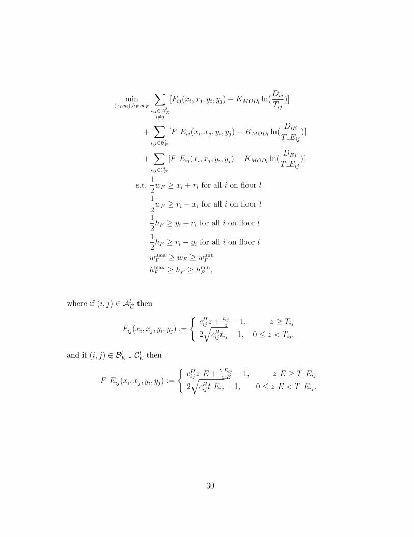
Stage Two: ModCoAR l

The ModCoAR l model is given next:

29

min(xi,yi),hF ,wF

∑i,j∈Al

Ei 6=j

[Fij(xi, xj, yi, yj)−KMODlln(

Dij

Tij)]

+∑i,j∈Bl

E

[F Eij(xi, xj, yi, yj)−KMODlln(

DiE

T Eij)]

+∑i,j∈Cl

E

[F Eij(xi, xj, yi, yj)−KMODlln(

DEj

T Eij)]

s.t.1

2wF ≥ xi + ri for all i on floor l

1

2wF ≥ ri − xi for all i on floor l

1

2hF ≥ yi + ri for all i on floor l

1

2hF ≥ ri − yi for all i on floor l

wmaxF ≥ wF ≥ wmin

F

hmaxF ≥ hF ≥ hmin

F ,

where if (i, j) ∈ AlE then

Fij(xi, xj, yi, yj) :=

{cHij z +

tijz− 1, z ≥ Tij

2√cHij tij − 1, 0 ≤ z < Tij,

and if (i, j) ∈ BlE ∪ ClE then

F Eij(xi, xj, yi, yj) :=

{cHij z E +

t Eij

z E− 1, z E ≥ T Eij

2√cHij t Eij − 1, 0 ≤ z E < T Eij.

30

Stage Three: BPL l

BPL l is formulated as:

min(xi,yi),hF ,wF

∑i,j∈Al

Ei 6=j

[cHij δ(xi, yi, xj, yj) +KBPLlXijYij]

+∑i,j∈Bl

E

[cHij δ(xi, yi, xE, yE)]

+∑i,j∈Cl

E

[cHij δ(xE, yE, xj, yj)]

s.t. Xij ≥1

2(wi + wj)− |xi − xj| for all (i, j) ∈ AlE, i 6= j

Yij ≥1

2(hi + hj)− |yi − yj| for all (i, j) ∈ AlE, i 6= j

Xij ≥ 0, Yij ≥ 0, and XijYij = 0, for all (i, j) ∈ AlE, i 6= j

1

2wF − (xi +

1

2wi) ≥ 0 for all i on floor l

(xi −1

2wi) +

1

2wF ≥ 0 for all i on floor l

1

2hF − (yi +

1

2hi) ≥ 0 for all i on floor l

(yi −1

2hi) +

1

2hF ≥ 0 for all i on floor l

wihi = ai, for all i on floor l

wmaxi ≥ wi ≥ wmin

i for all i on floor l

hmaxi ≥ hi ≥ hmin

i for all i on floor l

wmaxF ≥ wF ≥ wmin

F and hmaxF ≥ hF ≥ hmin

F .

Outline of FBF

The general outline of FBF is

Solve FAF;TotalCost=0;for l = 1 to K do

Solve ModCoAR l;Solve BPL l;TotalCost=TotalCost+BPLCost;

31

end forVerticalCost=

∑ij

cVij ∗ δ ∗ |yi − yj|;

TotalCost=TotalCost+VerticalCost;

4.3.2 AFS: Optimizing the Layout of Each Floor Simultaneously

Optimizing the layout of each floor simultaneously has the advantage of allowing for multi-ple elevator locations. AFS uses an extension of the ModCoAR and BPL methods denotedMulti-ModCoAR and Multi-BPL. Several notation modifications are made.

Additional Notation

The target distances are modified for the simultaneous case and are given as

t lij = αl(ri + rj)2, for all i, j on floor l and for all 1 ≤ l ≤ K.

The generalized target distances for each floor l are given as

T lij =√

t lijcij+ε

, for all i, j on floor l.

The M elevators are denoted E1, . . . , Em.

32

Stage 2: Multi-ModCoAR Model

min(xi,yi),hF ,wF

∑i,j on floor 1

i 6=j

[F 1ij(xi, xj, yi, yj)−KMOD1 ln(Dij

T 1ij)]

+∑

i,j on floor 2i 6=j

[F 2ij(xi, xj, yi, yj)−KMOD2 ln(Dij

T 2ij)]

+ . . .+∑

i,j on floor Ki 6=j

[F Kij(xi, xj, yi, yj)−KMODKln(

Dij

T Kij

)]

+∑i,j on

different floors

cHij Dij

s.t.1

2wF ≥ xi + ri and

1

2wF ≥ ri − xi for all i on floor 1

1

2hF ≥ yi + ri and

1

2hF ≥ ri − yi for all i on floor 1

1

2wF ≥ xi + ri and

1

2wF ≥ ri − xi for all i on floor 2

1

2hF ≥ yi + ri and

1

2hF ≥ ri − yi for all i on floor 2

...

1

2wF ≥ xi + ri and

1

2wF ≥ ri − xi for all i on floor K

1

2hF ≥ yi + ri and

1

2hF ≥ ri − yi for all i on floor K

wmaxF ≥ wF ≥ wmin

F

hmaxF ≥ hF ≥ hmin

F

Dij ≥ min (DiE1 +DE1j, DiE2 +DE2j, . . . , DiEm +DEmj) for all i, j not on same floor (?),

where if departments i and j are both on floor l

F lij(xi, xj, yi, yj) :=

{cHij z +

t lijz− 1, z ≥ T lij

2√cHij t lij − 1, 0 ≤ z < T lij

33

and recall that Dij = (xi − xj)2 + (yi − yj)

2 and thus DiE1 , for example, is the squaredistance between department i and elevator E1.

The constraints (?) are non-convex. Alternatively, the following convex constraints canbe used:

dij ≥√DiE1 +DE1j for all i, j on different floors

dij ≥√DiE2 +DE2j for all i, j on different floors

...

dij ≥√DiEK

+DEmj for all i, j on different floors,

with the objective function modified as:

min(xi,yi),hF ,wF

∑i,j on floor 1

i 6=j

[F 1ij(xi, xj, yi, yj)−KMOD1 ln(Dij

T 1ij)]

+∑

i,j on floor 2i 6=j

[F 2ij(xi, xj, yi, yj)−KMOD2 ln(Dij

T 2ij)]

+ . . .+∑

i,j on floor Ki 6=j

[F Kij(xi, xj, yi, yj)−KMODKln(

Dij

T Kij

)]

+∑i,j on

different floors

cHij(dij)2

Note that the model with convex constraints would probably yield a solution in whicheach circle will be not too far away from any elevator. The solution to Multi-ModCoARneed not be exact and although this may not give a uniform distribution of circles, it hasthe advantage of having convex constraints. The AFS model using the Multi-ModCoARmodel with convex constraints, denoted AFS-C, and the one using the Multi-ModCoARmodel with non-convex constraints, denoted AFS-NC, are tested and compared in Chapter5.

34

Stage 3: Multi-BPL Model

min(xi,yi),hF ,wF

∑i 6=j

(cHijd

Hij + cVijd

Vij

)+

∑i,j on floor 1

i 6=j

KBPL1XijYij

+∑

i,j on floor 2i 6=j

KBPL2XijYij + . . .+∑

i,j on floor Ki 6=j

KBPLKXijYij

s.t. Xij ≥1

2(wi + wj)− |xi − xj| and Yij ≥

1

2(hi + hj)− |yi − yj| for all i, j on floor 1

Xij ≥ 0, Yij ≥ 0, and XijYij = 0 for all i, j on floor 1

1

2wF − (xi +

1

2wi) ≥ 0 and (xi −

1

2wi) +

1

2wF ≥ 0 for all i on floor 1

1

2hF − (yi +

1

2hi) ≥ 0 and (yi −

1

2hi) +

1

2hF ≥ 0 for all i on floor 1

Xij ≥1

2(wi + wj)− |xi − xj| and Yij ≥

1

2(hi + hj)− |yi − yj| for all i, j on floor 2

Xij ≥ 0, Yij ≥ 0, and XijYij = 0 for all i, j on floor 2

1

2wF − (xi +

1

2wi) ≥ 0 and (xi −

1

2wi) +

1

2wF ≥ 0 for all i on floor 2

1

2hF − (yi +

1

2hi) ≥ 0 and (yi −

1

2hi) +

1

2hF ≥ 0 for all i on floor 2

...

Xij ≥1

2(wi + wj)− |xi − xj| and Yij ≥

1

2(hi + hj)− |yi − yj| for all i, j on floor K

Xij ≥ 0, Yij ≥ 0, and XijYij = 0 for all i, j on floor K

1

2wF − (xi +

1

2wi) ≥ 0 and (xi −

1

2wi) +

1

2wF ≥ 0 for all i on floor K

1

2hF − (yi +

1

2hi) ≥ 0 and (yi −

1

2hi) +

1

2hF ≥ 0 for all i on floor K

wihi = ai and wmaxi ≥ wi ≥ wmin

i and hmaxi ≥ hi ≥ hmin

i for all i

dHij = minEm:m=1...,M

(diEm + dEmj) for all i, j on different floors

dHij = dij for all i, j on same floor

wmaxF ≥ wF ≥ wmin

F and hmaxF ≥ hF ≥ hmin

F ,

35

where dij is simply the horizontal distance between departments i and j and, for example,diEm is the horizontal distance between department i and elevator Em.

Outline of Three-Stage Multi-Floor Layout Model (AFS)

The general outline of AFS is simply

Solve FAF;Solve Multi-ModCoAR;Solve Multi-BPL;

TotalCost=BPLCost;

36

Chapter 5

Computational Experiments

In this Chapter, we study the computational behavior of the proposed models. We also in-vestigate the choice of parameters, the effect of slack space, and the case of a narrow facility.Both versions of the three-stage multi-floor layout method are tested on several problemsusing the CPLEX 12.1.0 solver for the first stage and MINOS 5.4 for the remaining stagesthrough the GAMS modeling language. In addition, AFS using Multi-ModCoAR withthe convex constraints (AFS-C) will be compared to AFS with the non-convex constraints(AFS-NC). The test data used for the experiments are included in the Appendix.

Each problem requires an initial configuration of departments. The center of eachdepartment, (xi, yi), is placed at equal intervals around a circle of radius r = wmaxF +hmaxF .So, if there are M departments on a floor, then xi = r cos θi and yi = r sin θi whereθi = 2π(i− 1)/M .

5.1 Choosing Parameters

In this report, the choice of parameters was investigated in an attempt to find a correlationbetween these values and the quality of the optimal layout. The choice of αl and the penaltyvalues KMODl

and KBPLlare important to the performance of the modified ModCoAR and

BPL models in both versions of the proposed three-stage method described in Section 4.3:

• KBPLlmust be chosen large enough so that the method will converge to a feasible

layout.

• KMODlis a scaling parameter and affects the position of the circles in the layout.

– A small KMODlresults in a layout where the circles gather closer to the center

of the floor.

37

– A large KMODlresults in a layout where the circles are pushed further against

the walls of the floor.

• The parameter αl appears in the target distances of the modified ModCoAR models(tij = αl(ri + rj)

2), and can be viewed as a fine tuning parameter.

The effect of these parameters is illustrated in Figure 5.1 which is associated with Table5.1.

Figure 5.1: Solutions to ModCoAR for the Armour and Buffa 20-department problem.

Table 5.1: Parameters and Costs for Figure 5.1

Figure KMOD α Cost ofFinal Layout

Left 5 ∗∑

1≤i<j≤N

cij 7 4772.76

Center∑

1≤i<j≤N

cij 1.8 4743.20

Right 0.5 ∗∑

1≤i<j≤N

cij 0.5 4653.63

The method for finding several good layouts in [3] consists of a two step approach.First, KMOD and a large enough KBPL are chosen, then ModCoAR is run for severalvalues of α. The solutions are inspected and the one or two values, say α, for which a goodseparation of circles are observed, are chosen. The algorithm is then executed using valuesα± 0.1, 0.2, . . . , 0.5, usually resulting in several good layouts.

In the multi-floor case, different parameter values for each floor are often necessary toprovide good solutions. Due to the increased number of possible parameter combinationsit is even more desirable to have a mathematical method that can determine which penaltyvalues are likely to result in a good final layout. Anjos and Vannelli [3] observed that αhad a significant impact on the layouts obtained and, therefore, that the role of α shouldbe the subject of future research.

38

5.1.1 Investigating The Choice of Parameters KMOD and α

The aim of the ModCoAR model is for Dij ≈ Tij at optimality. My hypothesis was thata good approach for choosing parameters would be to choose KBPL large enough, and toadjust KMOD and α in such a way that the average of Dij/Tij would be approximately 1at optimality in hopes of discovering a correlation between Tij and the quality of the finalsolution. More precisely, the goal was to be able to adjust the parameters in such a waythat, on average, Dij ≈ Tij, say for parameter values α and KMOD, and then execute thecode for the values α = α± 0.1, 0.2, . . . , 0.5.

Although this method may find good layouts, having the average of Dij/Tij approxi-mately equal to 1 does not appear to be correlated to the best solutions. In fact, oftenthe best solutions are found far away from this point, demonstrating how difficult themulti-floor layout problem really is.

The results obtained using the Armour and Buffa 20-department problem and the 15-department and 3-floor problem were recorded for several values of KMOD. In particular,for each KMOD, the results for every value of alpha between 0.5 and 10 in intervals of0.1 were recorded. They clearly show that there seems to be no correlation between thegeneralized target distances and optimal costs. Figure 5.2 illustrates the best solution Ifound for the Armour and Buffa 20-department problem with aspect ratio constraints of3.0. Here, α = 8.0 and KMOD = 3 ∗

∑1≤i<j≤N cij. The average of

Dij

Tijis 10.46� 1 and it

can be seen that the circles are not well separated.

Figure 5.2: Results of ModCoAR and BPL for the lowest cost solution found.

Table 5.2 displays only some of the results obtained where it can be seen that oftenthe best solutions are found far away from the point at which Dij ≈ Tij on average. Theresults in the table are ordered by the average of Dij/Tij, from largest to smallest, so that itcan also be seen that as the average of Dij/Tij decreases, the total cost does not necessarydecrease as well.

39

Table 5.2: Generalized Target Distances vs. Total Costs: Armour and Buffa 20-DepartmentProblem

β?i KMOD KBPL α Average ofDij/Tij

Total Cost

3 5 ∗∑

1≤i<j≤N

cij

( ∑1≤i<j≤N

cij

)3

2.0 24.62 4649.31

3∑

1≤i<j≤N

cij

( ∑1≤i<j≤N

cij

)3

1.8 14.36 4743.20

3 5 ∗∑

1≤i<j≤N

cij

( ∑1≤i<j≤N

cij

)3

7 13.44 4772.76

3 3 ∗∑

1≤i<j≤N

cij

( ∑1≤i<j≤N

cij

)3

5.5 12.96 4531.80

3 3 ∗∑

1≤i<j≤N

cij

( ∑1≤i<j≤N

cij

)3

8.0 10.46 4127.80

3∑

1≤i<j≤N

cij

( ∑1≤i<j≤N

cij

)3

6 7.7 5003.579

3 3 ∗∑

1≤i<j≤N

cij

( ∑1≤i<j≤N

cij

)3

6.54 1.98 5920.42

5.2 Slack Space

The purpose of this section is to investigate the impact of the amount of slack space onthe quality of the solution. In particular, would even a small amount of slack increase thequality of the final solution?

To investigate this, I again used the Armour and Buffa 20-department problem, in whichthere is no slack space to begin with, and varied the amount of slack by expanding andcontracting the area of the floor. Some results are given in Tables 5.3 and 5.4. The entries ofthe table are the costs of the final layout and the columns, labeled 30/20, for example, meanthat the facility has a height of 30 and a width of 20. In Table 5.3, KBPL = (

∑1≤i<j≤N cij)

2,KMOD = 10 ∗

∑1≤i<j≤N cij, and there are no aspect ratio constraints. In Table 5.4,

KBPL = (∑

1≤i<j≤N cij)3, KMOD =

∑1≤i<j≤N cij, and the aspect ratio constraint for each

department is set to allow for a ratio less than or equal to 3.00. In both tables, the heightsand widths of each department are bounded below by 2.

In general, it can be seen that the more slack there is, the more likely it is that thesolver will find a feasible solution. It is also clear that there is a relationship between theamount of slack space and the layout cost. With more slack space, even though the solversometimes yields solutions that are much worse, often it does yield better solutions. For

40

example, in Tables 5.3 and 5.4, the lowest cost solution for each (highlighted in bold) arein the last column, meaning that they were found when there was the greatest amount ofslack space.

Table 5.3: Investigating Slack Space on Quality of Solution (no aspect ratio constraints)

α 30/20 30.1/20 30/20.1 30.1/20.1 30.1/20.2 30.2/20.1 30/21 31/21

1 - - - - - 5207.33 - 4240.291.5 4524.04 - 5520.07 - 4440.69 6005.1 4924.23 5023.782 - 5403.57 - 5247.08 5488.05 4981.41 4193.11 4720.79

2.5 5199.54 4978.23 5102.46 - 5055.52 5616.95 4878.7 4365.883 - 5238.6 4887.29 - 4621.24 5002.43 4625.01 3755.83

3.5 - - - 4864.42 4721.43 4528.89 5292.97 4458.934 5098.8 - 5145.08 - 4199.08 4923.42 4369.46 4836.86

4.5 - - 5238.37 - 4714.07 4252.66 4033.56 4483.485 - - 5468.68 - 5465.58 5137.25 4280.07 5151.61

slack 0 2 3 5.01 8.02 7.02 30 51

Table 5.4: Investigating Slack Space on Quality of Solution (aspect ratio constraints of 3.0)

α 30/20 30.1/20 30/20.1 30.1/20.1 30.1/20.2 30.2/20.1 30/21 31/21

1 - - - - 4677.23 4677.23 4902.85 4290.771.8 4743.196 - - - 4559.69 4559.69 4884.44 4850.741.5 - - - - 4663.04 4663.04 5326.51 4282.72 - - 4829.83 - - - 4966.86 4583.9

2.5 - - - - 5427.67 5427.67 5202.12 4607.424 - - 5391.84 - 5092.3 5092.3 5172.92 5007.43

5.1 5585.781 - 4283.31 - - - 4470.69 5128.825.2 5007.864 - - 4998.45 4735.8 4735.8 4297.3 4472.144.2 5019.872 - 4995.01 5639.81 - - 4735.48 5241.47

slack 0 2 3 5.01 8.02 7.02 30 51

5.3 Case of a Narrow Facility

When the shape of the facility is narrow, it can occur that the circles are too large to fitin the narrow facility causing the solution of ModCoAR (or of the modified ModCoARmodels) to be infeasible. In this case, it is possible to scale all of the radii by the same

41

amount so that the circles fit within the facility and a reasonable layout can be obtained.This is illustrated in Figures 5.3 and 5.4. The figures illustrate the layout of one floor ofthe 15-department and 3-floor problem solved using the proposed AFS-NC method. Thedata for this problem is given in Appendix A.2.

Figure 5.3: Infeasible solution of Multi-ModCoAR before scaling radii.

Figure 5.4: Solution of Multi-ModCoAR after radii is scaled by 0.8.

It is also sometimes helpful to scale the radii even when the solution is not infeasible,but the circles are too large for the narrowness of the facility.

5.4 Test Problem 1: 15-Departments and 3-Floors

The first test problem is a 15-department and 3-floor problem used in [5] to demonstrateMULTIPLE. It includes 6 potential lift locations that, from my understanding, are locatedon the perimeter of the floor and do not take up space. Department 15 is the receiv-ing/shipping department and is thus fixed to the first floor as a 5× 5 square in the bottomright hand corner. Also, because of the method used by MULTIPLE, a range of areas areallowed and the departments are not necessarily rectangular in shape. The final layoutcost determined by MULTIPLE is $125, 822.50 with compression and without any shape

42

Figure 5.5: Final layout obtained by MULTIPLE. The figure comes from [5].

constraints and is shown in Figure 5.5. This layout was found in 37.9 seconds. With shapeconstraints and further restrictions, the cost increases.

In order to be able to compare my results with theirs in the best way possible, Idetermined the areas of each department from MULTIPLE’s final layout. To do this, thefinal layout for each floor shown in Figure 5.5 was divided into a grid of unit squares. Thearea of a new rectangular department is precisely the number of unit squares occupied bythe irregularly shaped department. The exact problem data used is given Appendix A.2.

5.4.1 Application of FBF to Test Problem 1

In order to be able to apply FBF, I first considered the case where only one elevator locationis permitted. This location is fixed to the center of the floor and it is assumed that theelevator does not take up space, even though it can easily be made to do so. With theexception of the elevators, the specific data for this 15-department and 3-floor problem isthe same as the data given in Appendix A.2.

As is the case for FBF, the layout of each floor l was solved independently. The param-eters KMODl

and αl were varied to find a reasonable separation of circles in ModCoAR l,following the method described in Section 5.1. Table 5.5 summarizes the best results of20 different layouts, including the largest aspect ratios found on each floor, the cost of thefinal layout on each floor, the vertical cost, the total cost of the final layout, and also therunning time over all floors. It is possible to find lower cost solutions more easily if the

43

aspect ratio constraints are relaxed, but they were kept low to ensure realistically shapeddepartments. Note that the running time that is recorded is the running time for one run ofthe FBF code and does not take into consideration the time taken to tune the parametersbefore arriving at the combination of parameters that yields the solution.

Table 5.5: Results of FBF on Test Problem 1Largest Aspect Ratios

(Floor1, Floor2, Floor3)Cost

Floor 1Cost

Floor 2Cost

Floor 3Vertical

CostTotalCost

RunningTime (sec)

3.56, 3.00, 4.17 9958.91 15226.24 9736.50 86250 121,171.65 4.3813.13, 3.00, 4.17 7270.63 15226.24 9736.50 86250 118,483.37 4.4593.13, 3.00, 3.55 7270.63 15226.24 13939.16 86250 122,686.02 4.4802.50, 3.00, 3.55 10413.64 15226.24 13939.16 86250 125,829.03 4.353

Figure 5.6, illustrates one of the final layouts obtained. It can be seen that the proposedthree-stage multi-floor method found a low cost layout with realistic department shapes.

Figure 5.6: Final layout obtained by FBF.

5.4.2 Application of AFS to Test Problem 1

The same problem data was used, again with the exception that only one elevator locationis permitted, so that the AFS and FBF methods can be compared. Note that since thereis only one elevator location, there is no need to distinguish between AFS-C and AFS-NC.

The proposed AFS method was tested on this data for 20 different combinations ofparameter values. Slightly larger aspect ratio constraints were used than in Section 5.4.1in order to be able to find a few more feasible solutions in 20 trials. One reason for this

44

is that the method for choosing parameters as described in Section 5.1 works differentlywhen the layout of all floors are solved simultaneously because changing the parameterson one floor affects the layout of all floors. The feasible results of these trials are displayedin Table 5.6 and one of these layouts is illustrated in Figure 5.7.

Table 5.6: Results of AFS on Test Problem 1Largest Aspect Ratios

(Floor1, Floor2, Floor3)Cost

Floor 1Cost

Floor 2Cost

Floor 3Vertical

CostTotalCost

RunningTime (sec)

2.92, 5.2, 6.81 10341.97 15680.99 9033.54 86250 121,306.50 0.5235.12, 4.35, 4.6 11233.70 14168.26 13452.38 86250 125,104.35 0.5695.12, 4.52, 6.01 11233.70 14235.26 14494.89 86250 126,213.86 0.5525.64, 5.66, 4.33 13670.40 15586.55 15400.68 86250 130,907.63 0.516

Figure 5.7: Final Layout using AFS with a cost of 125,104.35.

5.4.3 Application of AFS to Test Problem 1- AFS-C vs. AFS-NC

This section compares the proposed AFS-C and AFS-NC methods. Both methods weretested on this 15-department and 3-floor problem (with all 6 elevators) using tight aspectratio constraints. First, KBPLl

, KMODl, and αl were chosen in such a way that a reasonable

solution to Multi-ModCoAR was achieved. Then αl was increased and decreased by thesame increments for both methods to find 30 different layouts. Table 5.7 displays thenumber of feasible solutions of the 30 trials and also the lowest cost found for each version.

The 4 lowest cost solutions for each method of the 30 trials are given in Tables 5.8and 5.9. It can be seen that both methods find good solutions without much difference incomputational times.

45

Table 5.7: AFS-C vs. AFS-NC

AFS-C AFS-NCAspect RatioConstraints

Floor1, Floor2, Floor3

# of SolutionsFound of 30

Lowest CostLayout

Running Timefor Lowest Cost

Layout

# of SolutionsFound of 30

Lowest CostLayout

Running Timefor Lowest Cost

Layout

5,5,5 3 126,936.07 0.929 12 133,181.78 0.9306,6,6 5 129,866.20 0.908 2 129,393.76 0.9128,8,8 12 126,754.52 0.926 13 123,501.51 0.870

Table 5.8: Results: AFS-CLargest Aspect Ratios

(Floor1, Floor2, Floor3) Total Cost RunningTime (sec)

2.66,8.00,4.32 126,754.52 0.9263.14,4.26,4.32 126,936.07 0.9297.14,7.15,4.32 128,982.77 0.9343.14,5.83,4.32 129,866.20 0.908

Table 5.9: Results: AFS-NCLargest Aspect Ratios

(Floor1, Floor2, Floor3) Total Cost RunningTime (sec)

7.06,4.42,5.76 123,501.53 0.8708.00,7.05,4.32 124,763.39 0.8697.14,4.63,3.54 125,269.47 0.8485.60,8.00,7.26 125,423.63 0.876

5.4.4 Comparing Proposed Methods to MFFLPE

Goetschalckx et al. [10] also use the 15 department, 3 floor, and 6 elevator problem totest their mathematical-programming method, MFFLPE, summarized in Section 2.1.4 ofthe literature review. They converted the irregularly shaped departments of the probleminto rectangular departments of the same area using one of the final layouts obtained fromMULTIPLE in [5]. Using their algorithm, they were able to find a “distance score” of121,419 in a time of 3,911 seconds.

However, there are a few issues with this. First of all, it is not clear what is meant bya “distance score”. Also, their algorithm requires the length of the long and short sides ofthe departments as input parameters rather than variables. In addition, it is clear fromtheir final layout shown in Figure 5.8 that department 15 is not fixed to the first floor asit should be.

I tested the proposed methods of this report using the same data that Goetschalckx

46

Figure 5.8: The optimal floor layout obtained by Goetschalckx et al. [10]. The figure was takenfrom [10].

et al. used in [10]. The data is the same as in Section A.2 of the Appendix except thatdepartment 15 is not fixed to the first floor and the areas are as given in Table 5.10.

Table 5.10: Fixed Area of DepartmentsDepartment 1 2 3 4 5 6 7 8 9 10 11 12 13 14 15

Area 15 10 9 7 10 25 25 15 9 25 10 15 6 19 25

First, FBF was applied to this data. In this case, it is assumed that there is only oneelevator location in the center of the floor. The largest aspect ratio in their results is 2.94.So, the aspect ratio constraints for each department in this experiment were set to allowfor ratios less than or equal to 2.94. The final layout is illustrated in Figure 5.9 with atotal cost of 106,830.08 and a total running time of 4.534 seconds.

Figure 5.9: The final layout obtained from FBF.

AFS-NC and AFS-C were also applied to this problem, taking all 6 elevators into con-sideration. The aspect ratio constraints were relaxed since it is more difficult to choose

47

parameters that will yield a feasible solution when the layout of all floors are solved simul-taneously. This is partly because changing a parameter on one floor affects the layout ofthe other floors as well. Another factor could be the multiple penalty terms in the objectivefunction. AFS-NC obtained a layout with a cost of 111,985.07 in 0.893 seconds and withaspect ratios of 4.00, 3.04, and 3.86. AFS-C obtained a layout with a cost of 113,803.39 in0.950 seconds and with aspect ratios of 4.00, 2.58, and 3.10.

From these results, it is clear that the proposed three-stage multi-floor method yieldsgood solutions and with small running times.

5.4.5 Comparison of Results for Test Problem 1

Although the results of the proposed three-stage multi-floor method cannot be compareddirectly to the final solution obtained by MULTIPLE because of differences in assumptionsand in the solution method, it is clear that FBF, AFS-C, and AFS-NC are able to findlow cost layouts with realistically shaped departments. MULTIPLE arrived at the solutionillustrated in Figure 5.5 in 37.9 seconds. All versions of the proposed method of this reportfind several high-quality layouts with running times of at most a few seconds. In particular,the AFS-C and AFS-NC methods find solutions to this problem in a running time of lessthan 1 second. One must keep in mind, however, that the time that is recorded here isthe running time for one run of the FBF, AFS-C, or AFS-NC code and does not take intoconsideration the time taken to tune the parameters before arriving at the combination ofparameters that yields the solution. Since, on average, only a few parameter combinationsneed to be tested before arriving at a solution, the proposed method can find solutions ina short amount of time. Of course this depends on the tightness of the constraints used.

It is clear that both the FBF and AFS methods can provide good quality solutions in ashort amount of time. Although FBF has the disadvantage of allowing for only one elevatorlocation, and it has slightly larger running times, often a high-quality layout can be foundin a more systematic way. This is because the layout of each floor is solved independently,so if the user finds that the layout on only one floor is not desirable, for example, theparameters for that floor can be changed without affecting the layout of the other floors.

Both the AFS-C and AFS-NC methods find good solutions without much difference inrunning times. From the results of Section 5.4.3, it may seem that AFS-NC yields lowercost solutions in general and that AFS-C finds lower cost solutions with lower aspect ratioconstraints. However, this may not be the case because these results were highly dependenton the parameters chosen for the particular experiment. It is likely that changing theparameters will find other high-quality solutions.

48

5.5 Test Problem 2: 40-Departments and 4-Floors

The second data set used is a 40-department, 4-floor, and 3-elevator problem found in [21].This test problem was designed for methods using grids and spacefilling curves, which is notthe case in the proposed method of this report. The grid size is 4.0 square distance unitsand I interpreted this to mean that each grid square of the floor is of size 2× 2. There are26 squares on the grid for each floor, implying a total area of 4× 26 = 104 square distanceunits. The inter-floor distance is 2.5 units and it seems as though department 40 is fixedto the first floor as an irregularly shaped department. This is illustrated in Figure 5.10.

There are several issues in comparing my results to the other methods in the literaturethat also used this test data, explaining why the costs I obtain in my results are muchlower than the costs of the others methods. It is my opinion that they cannot be compareddirectly. I fixed department 40 to the first floor, but I could not fix it in the same irregularshape as can be seen in Figure 5.10. In addition, the shape of the floor itself is irregular,but I assumed that it was a square floor of the same area. Since the grid size is 4.0 and theshape of each department must follow the shape of the grid squares, there is less flexibilityin the department shapes. The method of this report allows for rectangular shapes of anylength and width, allowing for more flexibility. The specific data used for the experimentis given in Appendix A.3.

Figure 5.10: The spacefilling curve and fixed department locations for the 40-departmentand 4-floor problem. Figure comes from [21].

49

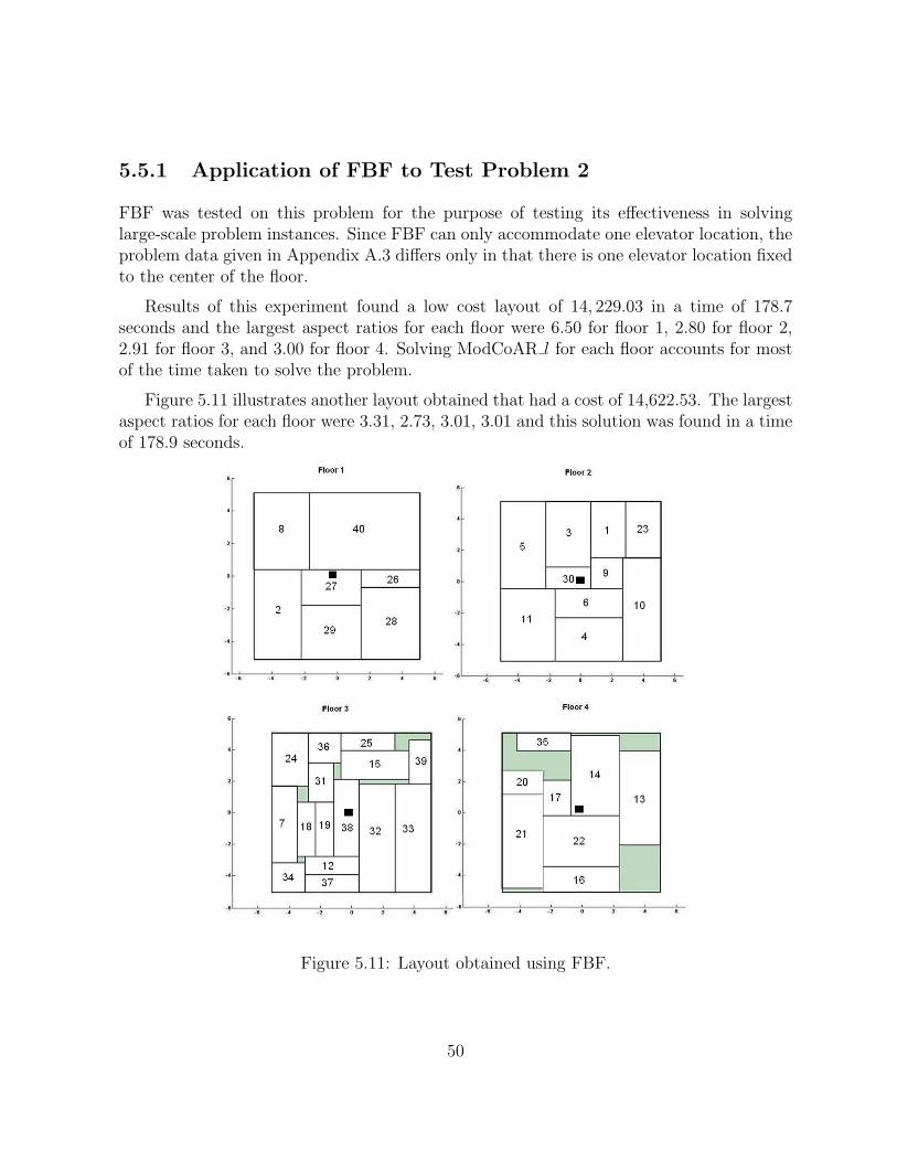
5.5.1 Application of FBF to Test Problem 2

FBF was tested on this problem for the purpose of testing its effectiveness in solvinglarge-scale problem instances. Since FBF can only accommodate one elevator location, theproblem data given in Appendix A.3 differs only in that there is one elevator location fixedto the center of the floor.

Results of this experiment found a low cost layout of 14, 229.03 in a time of 178.7seconds and the largest aspect ratios for each floor were 6.50 for floor 1, 2.80 for floor 2,2.91 for floor 3, and 3.00 for floor 4. Solving ModCoAR l for each floor accounts for mostof the time taken to solve the problem.

Figure 5.11 illustrates another layout obtained that had a cost of 14,622.53. The largestaspect ratios for each floor were 3.31, 2.73, 3.01, 3.01 and this solution was found in a timeof 178.9 seconds.

Figure 5.11: Layout obtained using FBF.

50

5.5.2 Application of AFS to Test Problem 2- AFS-C vs. AFS-NC

AFS-C and AFS-NC are tested on this problem, including all 3 elevators. Some resultsare given below in Tables 5.11 and 5.12, demonstrating that both methods are capable offinding good solutions to large problems very quickly.

Table 5.11: Results: AFS-CLargest Aspect Ratios

(Floor1, Floor2, Floor3) Horizontal Cost Vertical Cost Total Cost RunningTime (sec)

4.65, 6.50, 10.71, 11.00 9092.27 5562.50 14,654.77 2.824.15, 6.50, 5.90, 6.28 9369.99 5562.50 14,932.49 2.802.43, 5.78, 6.00, 2.69 9453.50 5562.50 15,016.00 2.734.50, 4.96, 5.34, 6.00 9501.68 5562.50 15,064.18 2.72

Table 5.12: Results: AFS-NCLargest Aspect Ratios

(Floor1, Floor2, Floor3) Horizontal Cost Vertical Cost Total Cost RunningTime (sec)

4.68, 2.77, 4.00, 5.00 8975.10 5562.50 14,537.60 2.684.48, 4.39, 4.00, 4.00 8959.16 5562.50 14,521.66 2.682.74, 3.61, 6.00, 3.69 8815.29 5562.50 14,377.79 2.663.47, 7.02, 6.38, 4.84 9633.63 5562.50 15,196.13 2.66

Note that choosing the initial configuration of departments (specifically for this data)using the method given in Chapter 5 results in the Multi-ModCoAR method being badlyscaled for some choices of parameters. However, both AFS-C and AFS-NC are still ableto find solutions, showing the strength of the methods. To avoid this problem, changeswere made to the initial configuration by randomly changing the position of some circles.The initial configuration and the specifics of the problem data are given in AppendixA.3. To avoid the problem of scaling for the application of the AFS-C method, the initialconfiguration was scaled by 0.3.

5.5.3 Comparison of Results for Test Problem 2

It is clear that each version of the proposed three-stage multi-floor method is capable offinding good layouts even for large problems. Also, both AFS-C and AFS-NC arrive ata solution in only a few seconds compared to the 200 seconds it takes FBF to arrive ata solution using the same problem data, except with only one elevator location. It seemsthat the difference in running time is due to the formulation of the objective function ofModCoAR l versus the objective function of Multi-ModCoAR.

51

5.6 Summary of Computational Experiments

First, the choice of parameters was investigated and although the aim of the ModCoARmodel is for Dij ≈ Tij at optimality, there seems to be no correlation between Tij andthe quality of the final solution. However, the method for choosing parameters by Anjosand Vannelli [3] presented in Section 5.1 resulted in many good layouts for the abovecomputational experiments.

It was seen that scaling the radii of the circles in the ModCoAR and the modifiedModCoAR models helps to achieve a reasonable layout of circles in the case of a narrowfacility.

The effect of slack space on the quality of the solution was also investigated. In general,the more slack there is, the more likely it is that the solver will find a feasible solution. Itis also clear that there is a relationship between the amount of slack space and the layoutcost; increasing the slack space often does yield better solutions.

From these test problems, it is clear that both the FBF and AFS methods can providegood quality solutions in a short amount of time. FBF has the disadvantage of allowingfor only one elevator location since the layout of the floors are solved independently ofone another. It also has larger running times than the AFS methods, but it seems thatthis is due to the formulation of the objective function of ModCoAR l versus the objectivefunction of Multi-ModCoAR. On the other hand, FBF has the advantage of allowing theuser to find a desirable layout in a more systematic way, often making it easier to find lowcost solutions with low aspect ratios.

The AFS methods, AFS-C and AFS-NC, solve the layout of all floors simultaneouslyand so have the advantage of allowing for multiple elevator locations. By adjusting theparameters α, KMODl

, KBPLl, the initial configuration, and aspect ratio constraints, both

AFS-C and AFS-NC yield good results and there is not much difference in running times.

52

Chapter 6

Conclusions and Future Research

In this report, a three-stage multi-floor layout method using mathematical-programmingtechniques was presented that provides good solutions to the multi-floor facility layoutproblem. The first stage is a linear mixed-integer program that assigns departments tofloors such that the total of the departmental interaction costs between floors is minimized.Subsequent stages find a locally optimal layout for each floor.

Two versions of this method were presented in detail. The first, FBF, solves the lay-out of each floor independently of the other floors and thus, allows for only one elevatorlocation. The second version, AFS, solves the layouts of all floors simultaneously, allowingfor multiple elevator locations. These versions were implemented, tested, and comparedto each other and to existing results in the literature through computational experiments.From the results of the experiments, it is clear that both versions can provide high-qualitysolutions to the multi-floor layout problem even for large problem instances.

Not only does the proposed method achieve very good results, but it also overcomessome limitations that are present in previous methods. For example, departments are notsplit across floors, multiple elevator locations are allowed with the AFS version, and therunning times are small. The method can find several very good layouts for the sameproblem in a short time by simply changing the parameters αl, KMODl

, and KBPLlas

opposed to other methods that find only one optimal layout. Low cost layouts with realisticdepartment shapes can be found by controlling the aspect ratio of each department throughconstraints.

It is clear that the initial configuration of departments, and the parameters αl, KMODl,

and KBPLlhave a large impact on the quality of the final solution. It is fairly easy to find

a combination of these values that yield good solutions, but it is not clear ahead of timewhich combination it will be. The choice of these values could be the subject of futureresearch. Future work could also involve constructing a single-stage method that assigns

53

departments to floors and optimizes the layout on each floor using the same underlyingconcepts of the proposed method of this report. Lastly, to find the closest elevator for eachdepartment in the Multi-BPL model, the “min” function was used, which is believed to beproblematic. No problems were noticed in the computational experiments of this report,but replacing this function could be the subject of future research.

54

APPENDIX

55

Appendix A

Test Data for ComputationalExperiments

A.1 Data for the Armour and Buffa 20-Department

Problem

• The height of the facility is 30 and the width is 20.

Table A.1: Initial Configuration for Armour and Buffa 20-Department ProblemDepartment Center Department Center

1 (155.12000000, 0.00000000) 11 (44.13591924,148.70855736)2 (153.84646694,19.83630532) 12 (24.75713572,53.13163824)3 (150.04677915,39.34689906) 13 (4.97184071,155.04030186)4 (143.78332740,58.21141780) 14 (14.89509178,154.40320800)5 (135.15895738,76.12010667) 15 (-34.51744728,151.23081774)6 (124.31528102,92.77890549) 16 (-53.57302724,145.57522163)7 (111.43035119,107.91427725) 17 (-71.74893958,137.52928440)8 (96.71573806,121.27769956) 18 (-88.74673632,127.22512013)9 (80.41305520,132.64974540) 19 (-104.28731410,114.83192291)10 (62.78999219,141.84368608) 20 (-118.11549706,100.55318868)

56

Table A.2: Costs for Armour and Buffa 20-Department Problem

1 2 3 4 5 6 7 8 9 10 11 12 13 14 15 16 17 18 19 20

1 0 1.8 1.2 0 0 0 0 0 0 1.041.12 0 0 1.20 0 0 0 0 0 02 1.8 0 0.96 24.450.78 0 13.95 0 1.201.35 0 0 0 0 0 0 0 0 6.90 03 1.2 0.96 0 0 0 2.21 0 0 3.153.90 0 0 0 13.05 0 0 0 0 13.65 04 0 24.45 0 0 1.085.70 7.50 0 2.34 0 0 1.40 0 0 0 0 0 1.5015.75 05 0 0.78 0 1.08 0 0 2.25 1.35 0 1.56 0 0 0 0 1.35 0 0 0 0 06 0 0 2.21 5.70 0 0 6.15 0 0 0 0 0.45 0 0 0 0 0 1.05 0 07 0 13.95 0 7.50 2.256.15 0 24.00 0 1.87 0 0 0 0.96 0 0 0 1.65 0 3.758 0 0 0 0 1.35 0 24.0 0 0 0 0 0 0.60 0 0 0 0 0 7.50 33.459 0 1.20 3.15 2.34 0 0 0 0 0 0 0 0 0 7.50 0 0 7.50 0 0 0101.04 1.35 3.90 0 1.56 0 1.87 0 0 0 0.3612.0 0 18.6 1.92 0 0 0 5.25 0111.12 0 0 0 0 0 0 0 0 0.36 0 2.25 0 3.00 0.9622.50 0 0 0 012 0 0 0 1.40 0 0.45 0 0 0 12.02.25 0 0 0 1.65 0 15.00 0 8.40 013 0 0 0 0 0 0 0 0.60 0 0 0 0 0 8.00 1.04 6.00 0 0 0 0141.20 0 13.05 0 0 0 0.96 0 7.5018.63.00 0 8.00 0 9.75 0 0 0.90 0 05 0 0 0 0 1.35 0 0 0 0 1.920.961.651.04 9.75 0 0 5.25 0 0 016 0 0 0 0 0 0 0 0 0 0 2.25 0 6.00 0 0 0 12.00 0 0 017 0 0 0 0 0 0 0 0 7.50 0 0 15.0 0 0 5.2512.00 0 0 7.50 018 0 0 0 1.50 0 1.05 1.65 0 0 0 0 0 0 0.90 0 0 0 0 4.65 019 0 6.90 13.6515.75 0 0 0 7.50 0 5.25 0 8.40 0 0 0 0 7.50 4.65 0 020 0 0 0 0 0 0 3.75 33.45 0 0 0 0 0 0 0 0 0 0 0 0

Table A.3: Fixed Area of Departments for Armour and Buffa 20-Department Problem

Department 1 2 3 4 5 6 7 8 9 10 11 12 13 14 15 16 17 18 19 20

Area 27 18 27 18 18 18 9 9 9 24 60 42 18 24 27 75 64 41 27 45

57

A.2 Data for 15-Department and 3-Floor Problem

• There are 15 departments and 3 floors.

• There are 6 elevator locations. They are located at (-7.5,0), (-2.5,2.5), (2.5,2.5),(7.5,0), (2.5,-2.5), and (-2.5,-2.5).

• Department 15 is the receiving/shipping department and is thus fixed to the firstfloor as a 5× 5 square in the bottom right hand corner.

• Departments are assumed to be rectangular.

• The initial configuration of departments for floor number l were determined from theformulas xi = r cos θi, yi = r sin θi, where r = wmaxF + hmaxF and θi = 2π(i − 1)/M ,and M is the number of departments on floor l.

• The maximum area for each floor is 75 where wmaxF = 15 and hmaxF = 5.

• The distance between any two adjacent floors is 10.

• The radii is scaled by .8 (narrow facility).

Table A.4: Vertical Cost for 15-Department and 3-Floor Problem

1 2 3 4 5 6 7 8 9 10 11 12 13 14 15

1 5 5 5 5 5 5 5 5 5 5 5 5 5 5 1.252 5 5 5 5 5 5 5 5 5 5 5 5 5 5 1.253 5 5 5 5 5 5 5 5 5 5 5 5 5 5 1.254 5 5 5 5 5 5 5 5 5 5 5 5 5 5 1.255 5 5 5 5 5 5 5 5 5 5 5 5 5 5 1.256 5 5 5 5 5 5 5 5 5 5 5 5 5 5 1.257 5 5 5 5 5 5 5 5 5 5 5 5 5 5 1.258 5 5 5 5 5 5 5 5 5 5 5 5 5 5 1.259 5 5 5 5 5 5 5 5 5 5 5 5 5 5 1.2510 5 5 5 5 5 5 5 5 5 5 5 5 5 5 1.2511 5 5 5 5 5 5 5 5 5 5 5 5 5 5 1.2512 5 5 5 5 5 5 5 5 5 5 5 5 5 5 1.2513 5 5 5 5 5 5 5 5 5 5 5 5 5 5 1.2514 5 5 5 5 5 5 5 5 5 5 5 5 5 5 1.2515 1.25 1.25 1.25 1.25 1.25 1.25 1.25 1.25 1.25 1.25 1.25 1.25 1.25 1.25 1.25

58

Table A.5: Flow Matrix for 15-Department and 3-Floor Problem

1 2 3 4 5 6 7 8 9 10 11 12 13 14 15

1 0 0 0 0 0 0 0 0 0 0 0 0 0 0 2402 240 0 0 0 0 0 0 0 0 0 0 0 0 0 03 0 0 0 1200 0 0 0 0 0 0 0 0 0 0 04 0 0 0 0 0 0 0 0 0 1200 0 0 0 0 05 0 0 0 0 0 0 0 0 0 0 0 0 0 600 06 0 0 0 0 0 0 0 480 0 0 0 0 0 0 07 0 0 0 0 0 0 0 480 0 0 0 0 0 0 08 0 0 0 0 0 0 0 0 0 0 0 0 0 0 1209 0 0 0 0 0 0 0 0 0 600 0 0 0 0 010 0 0 0 0 0 0 0 0 0 0 0 600 0 0 011 0 0 0 0 0 0 480 0 0 0 0 0 0 0 012 0 0 0 0 0 0 0 0 0 0 0 0 0 0 60013 0 0 0 0 0 0 480 0 0 0 0 0 0 0 014 0 0 0 0 0 0 0 0 0 0 0 600 0 0 015 0 10 25 0 25 40 0 0 25 0 40 0 20 0 0

Table A.6: Horizontal Costs for 15-Department and 3-Floor Problem

1 2 3 4 5 6 7 8 9 10 11 12 13 14 15

1 0 1 1 1 1 1 1 1 1 1 1 1 1 1 0.252 1 0 1 1 1 1 1 1 1 1 1 1 1 1 0.253 1 1 0 1 1 1 1 1 1 1 1 1 1 1 0.254 1 1 1 0 1 1 1 1 1 1 1 1 1 1 0.255 1 1 1 1 0 1 1 1 1 1 1 1 1 1 0.256 1 1 1 1 1 0 1 1 1 1 1 1 1 1 0.257 1 1 1 1 1 1 0 1 1 1 1 1 1 1 0.258 1 1 1 1 1 1 1 0 1 1 1 1 1 1 0.259 1 1 1 1 1 1 1 1 0 1 1 1 1 1 0.2510 1 1 1 1 1 1 1 1 1 0 1 1 1 1 0.2511 1 1 1 1 1 1 1 1 1 1 0 1 1 1 0.2512 1 1 1 1 1 1 1 1 1 1 1 0 1 1 0.2513 1 1 1 1 1 1 1 1 1 1 1 1 0 1 0.2514 1 1 1 1 1 1 1 1 1 1 1 1 1 0 0.2515 0.25 0.25 0.25 0.25 0.25 0.25 0.25 0.25 0.25 0.25 0.25 0.25 0.25 0.25 0

59

Table A.7: Fixed Area of Departments for 15-Department and 3-Floor ProblemDepartment 1 2 3 4 5 6 7 8 9 10 11 12 13 14 15

Area 12 7 6 5 8 27 26 16 22 22 10 14 6 18 25

A.3 Data for 40-Department and 4-Floor Problem

• There are 40 departments and 4 floors.

• There are 3 elevators locations given by (−√

26, 0), (0,√

26), and (√

26, 0).

• cHij = 1 and cVij = 5 for all i 6= j.

• The distance between adjacent floors is 25 distance units.

• The area of each floor is 104.

• Department 40 is fixed to the first floor.

Table A.8: Flow Data for 40-Department and 4-Floor ProblemFrom→To

Department Flow From→ToDepartment Flow From→To

Department Flow From→ToDepartment Flow

1→3 66.25 5→15 10 16→17 10 32→33 251→5 101.25 5→23 6 17→13 5 33→34 251→9 40 5→34 25 18→19 5 34→2 12.51→12 4 6→11 20 19→3 5 36→37 101→30 25 6→23 12 20→21 15 37→32 251→36 12.5 6→29 17.5 21→22 15 38→39 251→38 10 7→24 15 22→23 7.5 39→33 252→40 23.75 8→2 17.5 23→8 7.5 40→1 149.53→4 70 8→40 15 24→25 7.5 40→7 7.54→10 40 9→10 40 25→22 7.5 40→16 44→14 5 10→11 16 26→27 17.5 40→18 44→25 7.5 11→2 16 27→28 8.75 40→20 64→28 17.5 12→13 2 28→29 8.75 40→26 74→33 25 13→14 10 29→8 8.755→6 78.75 14→15 5 30→31 12.55→11 40 15→2 4 31→32 12.5

60

Table A.9: Initial Configuration for 40-Department and 4-Floor ProblemDepartment Center Department Center

1 ( 10.000000 ,0.000000) 21 ( -10.000000, 0.000000 )2 ( 9.876883, 1.564345 ) 22 ( -9.876883, -1.564345 )3 ( 9.510565, 3.090170 ) 23 ( -9.510565, -3.090170 )4 ( 8.910065, 4.539905 ) 24 ( -8.910065, -4.539905 )5 ( 8.090170, 5.877853 ) 25 ( -8.090170, -5.877853 )6 ( 7.071068, 7.071068 ) 26 ( -7.071068, -7.071068 )7 ( 5.877853, 8.090170 ) 27 ( -5.877853, -8.090170 )8 ( 4.539905, 8.910065 ) 28 ( -4.539905, -8.910065 )9 (3.090170, 9.510565 ) 29 ( -3.090170, -9.510565 )10 ( 1.564345, 9.876883 ) 30 ( -1.564345, -9.876883 )11 ( 0.000000, 10.000000 ) 31 ( -0.000000, -10.000000 )12 (-1.564345, 9.876883 ) 32 ( 1.564345, -9.876883 )13 ( -3.090170, 9.510565 ) 33 ( 3.090170, -9.510565 )14 (-4.539905, 8.910065 ) 34 ( 4.539905, -8.910065 )15 ( -5.877853, 8.090170 ) 35 ( 5.877853, -8.090170 )16 ( -7.071068, 7.071068 ) 36 ( 7.071068, -7.071068 )17 ( -8.090170, 5.877853 ) 37 ( 8.090170, -5.877853 )18 ( -8.910065, 4.539905 ) 38 ( 8.910065, -4.539905 )19 ( -9.510565, 3.090170 ) 39 ( 9.510565, -3.090170 )20 ( -9.876883, 1.564345 ) 40 ( 9.876883, -1.564345 )

Table A.10: Fixed Area of Departments for 40-Department and 4-Floor Problem

Department 1 2 3 4 5 6 7 8 9 10 11 12 13 14 15 16 17 18 19 20

Area 8 16 12 12 16 8 8 16 4 16 16 4 16 16 8 8 4 4 4 4

Department 21 22 23 24 25 26 27 28 29 30 31 32 33 34 35 36 37 38 39 40

Area 16 16 8 8 4 4 8 16 12 4 4 16 16 4 4 4 4 8 4 32

Note that in order to deal with one of the methods being badly scaled for this problem,the initial configuration for the problem was not obtained by using the method describedin 5, rather the position of some circles were changed randomly.

61

Bibliography

[1] Sue Abdinnour-Helm and Scott W. Hadley. Tabu search based heuristics for multi-floor facility layout. International Journal of Production Research, 38(2):365–383,2000. 13, 14, 24

[2] Miguel F. Anjos and Anthony Vannelli. An attractor-repeller approach to floorplan-ning. Mathematical Methods of Operations Research, 56:3–27, 2002. 19, 20

[3] Miguel F. Anjos and Anthony Vannelli. A new mathematical-programming frameworkfor facility-layout design. INFORMS J. on Computing, 18(1):111–118, 2006. ix, 1, 2,15, 16, 17, 18, 19, 20, 21, 22, 23, 28, 38, 52

[4] Yavuz A. Bozer and Russell D. Meller. A construction-type layout algorithm formulti-floor facilities with capacitated lifts. Technical report, University of Michiganand Auburn University, 1992. 11, 12, 13

[5] Yavuz A. Bozer, Russell D. Meller, and Steven J. Erlebacher. An improvement-typelayout algorithm for single and multiple-floor facilities. Manage. Sci., 40(7):918–932,1994. ix, 4, 5, 7, 24, 42, 43, 46

[6] Elwood S. Buffa, Gordon C. Armour, and Thomas E. Vollmann. Allocating facilitieswith CRAFT. Harvard Business Review, 42(2):136 – 158, 1964. 3

[7] Chir-Ho Chang, Jin-Ling Lin, and Huei-Jiun Lin. Multiple-floor facility layout designwith aisle construction. IEMS, 5:1–10, 2006. 7

[8] Zvi Drezner. DISCON: A new method for the layout problem. Operations Research,28(6):1375–1384, 1980. 15, 16

[9] Thomas A. Feo and Mauricio G.C. Resende. Greedy randomized adaptive searchprocedures. Journal of Global Optimization, 6:109–133, 1995. 13

[10] Marc Goetschalckx and Takashi Irohara. Efficient formulations for the multi-floorfacility layout problem with elevators. School of Industrial and Systems EngineeringResearch Report, 2007. ix, 9, 46, 47

62

[11] Eric S. Grajo and Yavuz A. Bozer. LayOPT: A data driven facilities layout optimiza-tion system for engineers. http://www.pmcorp.com/PublishedPapers/Simulation%20Publications/Sim-Layout,% 20Material% 20Handling% 20and% 20Warehous-ing/LayOPTADataDrivenFacilities.pdf. 5

[12] Peter Hahn, J. MacGregor Smith, and Yi-Rong Zhu. The multi-story space assignmentproblem. Annals of Operations Research, 2008. 1, 9

[13] Roger V. Johnson. SPACECRAFT for multi-floor layout planning. ManagementScience, 28(4):407–417, 1982. 4

[14] Bharat K. Kaku, Thomas E. Morton, and Gerald L. Thompson. A heuristic methodfor the facilities layout problem. Working paper, 1987. 11

[15] Bharat K. Kaku, Gerald L. Thompson, and Ilker Baybars. A heuristic method for themulti-story layout problem. European Journal of Operational Research, 37(3):384 –397, 1988. 10, 11

[16] Jasmit Kochhar and Sunderesh S. Heragu. MULTI-HOPE: A tool for multiple floorlayout problems. International Journal of Production Research, 36:3421–3435(15),1998. 6, 7, 10

[17] Kyu-Yeul Lee, Myung-Il Roh, and Hyuk-Su Jeong. An improved genetic algorithmfor multi-floor facility layout problems having inner structure walls and passages.Computers & Operations Research, 32(4):879 – 899, 2005. 7

[18] Robin S. Liggett and William J. Mitchell. Optimal space planning in practice.Computer-Aided Design, 13(5):277 – 288, 1981. Special Issue Design Optimization. 8

[19] Zhi-Quan Luo, Jong-Shi Pang, and Daniel Ralph. Mathematical Programs with Equi-librium Constraints. Cambridge University Press, Cambridge, UK, 1996. 22

[20] Kenichiro Matsuzaki, Takashi Irohara, and Kazuho Yoshimoto. Heuristic algorithmto solve the multi-floor layout problem with the consideration of elevator utilization.Computers & Industrial Engineering, 36(2):487 – 502, 1999. 7

[21] Russell D. Meller and Yavuz A. Bozer. Solving the facility layout problem with sim-ulated annealing. Technical Report 91-20, Department of Industrial & OperationsEngineering, University of Michigan, 1991. ix, 49

[22] Russell D. Meller and Yavuz A. Bozer. A new simulated annealing algorithm for thefacility layout problem. International Journal of Production Research, 34(6):1675–1692, 1996. 5, 6, 24

63

[23] Russell D. Meller and Yavuz A. Bozer. Alternative approaches to solve the multi-floorfacility layout problem. Journal of Manufacturing Systems, 16(3):192 – 203, 1997. 2,9, 10, 12, 13, 24, 25, 26, 27

[24] Russell D. Meller and Kai-Yin Gau. The facility layout problem: Recent and emergingtrends and perspectives. Journal of Manufacturing Systems, 15(5):351 – 366, 1996. 4

[25] Jerrold M. Seehof, Wayne O. Evans, James W. Friederichs, and James J. Quigley.Automated facilities layout programs. In Proceedings of the 1966 21st national con-ference, pages 191–199, New York, NY, USA, 1966. ACM. 11

[26] Drew J. van Camp, Michael W. Carter, and Anthony Vannelli. A nonlinear optimiza-tion approach for solving facility layout problems. European Journal of OperationalResearch, 57(2):174–189, March 1992. 16

64