A Three-Factor Yield Curve Model: Non-A–ne Structure, …fdiebold/papers/paper60/djl.pdf · Non-A–ne Structure, Systematic Risk Sources, and ... Systematic Risk Sources, and Generalized

A Three-Factor Yield Curve Model:

Non-Affine Structure, Systematic Risk Sources, and

Generalized Duration∗

Francis X. DieboldUniversity of Pennsylvania and NBER

Lei JiUniversity of Pennsylvania

Canlin LiUniversity of California-Riverside

March 9, 2004

AbstractWe assess and apply the term-structure model introduced by Nelson and Siegel (1987)and re-interpreted by Diebold and Li (2003) as a modern three-factor model of level,slope and curvature. First, we ask whether the model is a member of the affine class,and we find that it is not. Hence the poor forecasting performance recently documentedfor affine term structure models in no way implies that our model will forecast poorly,which is consistent with Diebold and Li’s (2003) finding that it indeed forecasts quitewell. Next, having clarified the relationship between our three-factor model and theaffine class, we proceed to assess its adequacy directly, by testing whether its level, slopeand curvature factors do indeed capture systematic risk. We find that they do, andthat they are therefore priced. Finally, confident in the ability of our three-factor modelto capture the pricing relations present in the data, we proceed to explore its efficacyin bond portfolio risk management. Traditional Macaulay duration is appropriate onlyin a one-factor (level) context; hence we move to a three-factor generalized duration,and we show the superior performance of hedges constructed using it.

Contact author:Professor Canlin LiGraduate School of ManagementUniversity of CaliforniaRiverside, CA [email protected] (909) 787 2325fax (909) 787 3970

∗Acknowledgments: This paper is dedicated to the memory of our teacher and colleague, Albert Ando.We thank Lawrence R. Klein for helpful editorial comments, but we alone are responsible for any remainingerrors. We are grateful to the Guggenheim Foundation and the National Science Foundation for researchsupport.

1

Diebold, F.X., Ji, L. and Li, C. (2006),"A Three-Factor Yield Curve Model: Non-Affine Structure, Systematic Risk Sources, and Generalized Duration,"

in L.R. Klein (ed.),Long-Run Growth and Short-Run Stabilization: Essays in Memory of Albert Ando. Cheltenham, U.K.:Edward Elgar, 240,274.

1 Introduction

We assess and apply the term-structure model introduced by Nelson and Siegel (1987) and

re-interpreted by Diebold and Li (2003) as a modern three-factor model of level, slope and

curvature. Our assessment and application has three components. First, we ask whether the

model is a member of the recently-popularized affine class, and we find that it is not. Hence

the poor forecasting performance recently documented for affine term structure models (e.g.,

Duffee, 2002) in no way implies that our model will forecast poorly, which is consistent with

Diebold and Li’s (2003) finding that it indeed forecasts quite well.

Second, having clarified the relationship between our three-factor model and the affine

class, we proceed to assess its adequacy directly, by asking whether its level, slope and

curvature factors capture systematic risk. We find that they do, and that they are therefore

priced. In particular, we show that the cross section of bond returns is well-explained by the

sensitivities (loadings) of the various bonds to the level, slope and curvature state variables

(factors).

Finally, confident in the ability of our three-factor model to capture the pricing relations

present in the data, we proceed to explore its use for bond portfolio risk management.

Traditional Macaulay duration is appropriate only in a one-factor (level) context; hence we

move to a three-factor generalized duration vector suggested by our model. By matching all

components of generalized duration, we hedge against level risk, slope risk, and curvature

risk. Traditional Macaulay duration hedging, which hedges only level risk, emerges as a

special and highly-restrictive case. We compare the hedging performance of our generalized

duration to that of several existing competitors, and we find that it compares favorably.

We proceed as follows. In section 2 we review affine term structure models and study

their relationship to our three-factor model. In section 3 we test whether our level, slope

and curvature factors represent priced systematic risks, and we ask whether they successfully

explain the cross section of bond returns. In section 4 we extend Macaulay duration to a

generalized vector duration and study its properties and immunization performance. We

1



conclude in section 5.

2 Is the Three-Factor Model Affine?

Affine term structure models have recently gained great popularity among theorists (e.g., Dai

and Singleton, 2000), due to their charming simplicity. Ironically, however, Duffee (2002)

shows that the restrictions associated with affine structure produce very poor forecasting

performance. A puzzle arises: the Nelson-Siegel (1987) and Diebold-Li (2003) three-factor

term structure model appears affine, yet it forecasts well. Here, we resolve the puzzle.

2.1 Background

A little background on Nelson-Siegel (1987) is required to understand what follows. Nelson

and Siegel proposed the parsimonious yield curve model,

yt(τ) = b1t + b2t1− e−λtτ

λtτ− b3te

−λtτ . (1)

where yt(τ) denotes the continuously-compounded zero-coupon nominal yield at maturity

τ , and b1t, b2t, b3t, and λt are (time-varying) parameters. The Nelson-Siegel model can

generate a variety of yield curve shapes including upward sloping, downward sloping,

humped, and inversely humped, but it can not generate yield curves with two or more

local minima/maxima that are sometimes (though rarely) observed in the data.

Diebold and Li (2003) reformulated the original Nelson-Siegel expression as

yt(τ) = f1t + f2t1− e−λτ

λτ+ f3t

(1− e−λτ

λτ− e−λτ

). (2)

The advantage of the Diebold-Li representation is that we can easily give economic

interpretations to the parameters f1t, f2t, and f3t. In particular, we can interpret them

as a level factor, a slope factor, and a curvature factor, respectively. To see this, note that

2



the loading on f1t is 1, a constant that doesn’t depend on the maturity. Thus f1t affects

yields at different maturities equally and hence can be regarded as a level factor. The loading

associated with f2t is (1− e−λτ )/λτ , which starts at 1 but decays monotonically to 0. Thus

f2t affects primarily short-term yields and hence changes the slope of the yield curve. Finally,

factor f3t has loading (1 − e−λτ )/λτ − e−λτ , which starts at 0, increases, and then decays.

Thus f3t has largest impact on medium-term yields and hence moves the curvature of the

yield curve. In short, based on (2), we can express the yield curve at any point of time as

a linear combination of the level, slope and curvature factors, the dynamics of which drive

the dynamics of the entire yield curve.

In the original Nelson-Siegel formulation, the parameter λt may change with time. But

as argued in Diebold and Li (2003), we can treat it as fixed with little degradation of fit (they

fix λ at 0.0609 with maturities measured in months). This treatment greatly simplifies the

estimation procedure, and even more importantly, it sharpens economic intuition, because

λt has no obvious economic interpretation. After fixing λt, it is trivial to estimate f1t, f2t,

and f3t from equation (2) via ordinary least squares (OLS) regressions.

In the empirical work that follows we use the Center for Research in Security Prices

(CRSP) monthly treasury file to extract the three factors. For liquidity and data quality

considerations, we keep only bills with maturity longer than 1 month and notes/bonds with

maturity longer than 1 year (see also Bliss, 1997). In the first step, as in Fama and Bliss

(1987), we use a bootstrap method to infer zero bond yields from available bill, note, and

bond prices. In the second step, we treat the factor loadings in the above equation as

regressors and we fix λ = 0.0609 to calculate the regressor values for each zero bond. In the

third step, we run a cross-sectional regression of the zero yields on the calculated regressor

values. The regression coefficients f̂1t, f̂2t, and f̂3t are the estimated factor values. We do

this in each month to get the time series of three factors, which we display in Figure 1

from 1972 to 2001. In Figure 2, we show a few selected term structure scenarios. Both

the bootstrapped zero yields and the three-factor fitted yield curves are included. From the

3



graph, it’s clear that the fitted curves can reproduce raw zero yields very well, at both the

short and long ends of the curve1.

2.2 Analysis

Even a casual look at equation (2) reveals that the yield is affine in the three factors. This

raises a natural question: is our model related to the affine term structure models popular

in the literature? In particular, can we show that the Nelson-Siegel model is an affine term

structure model (ATSM), in the sense of Duffie and Kan (1996), Dai and Singleton (2000),

and Piazessi (2002)? As in Dai and Singleton (2000), an N -factor general ATSM has the

following elements:

The state variable Y (t), an N × 1 vector, follows the affine diffusion,

dY (t) = K̃(θ̃ − Y (t))dt + Σ√

S(t)dW̃ (t), (3)

where W̃ (t) is an N -dimensional independent standard Brownian motion, K̃ and Σ are N×N

matrices, θ̃ is an N × 1 vector, and S(t) is a diagonal matrix with the ith diagonal element

[S(t)]ii = αi + β′iY (t).

The time t price of a zero-coupon bond with maturity τ is

P (t, τ) = exp(A(τ)−B(τ)′Y (t)), (4)

1Note that Fama and Bliss consider only yields on bonds with maturities up to five years. As a result, muchinformation contained in the long end of the yield curve is lost. Similarly, Diebold and Li (2003) consideronly yields with maturities up to ten years. Because we want to distill as much information as possible fromthe entire yield curve, in this paper we use all non-callable government bonds in the bootstrapping exercise.

4



where A(τ) and B(τ) are solutions to the ordinary differential equations (ODEs),

dA(τ)

dτ= −θ̃

′K̃ ′B(τ) +

1

2

N∑i=1

(Σ′B(τ))2i αi − δ0 (5)

dB(τ)

dτ= −K̃ ′B(τ)− 1

2

N∑i=1

(Σ′B(τ))2i βi + δy, (6)

with initial conditions

A(0) = 0; B(0) = 0. (7)

From (4), it is straightforward to express bond yields as

yt(τ) = −1

τln(P (t, τ)) = −A(τ)

τ+

B(τ)′Y (t)

τ. (8)

Dai and Singleton (2000) give a canonical representation for the ATSM, in which each

ATSM with N factors can be uniquely classified as Am(N), where m is the number of state

variables entering the variance of the diffusion term S(t). The most general (maximal) form

of the canonical representation is

K =

Km×m 0m×(N−m)

K(N−m)×m K(N−m)×(N−m)

(9)

θ =

θm×1

0(N−m)×1

Σ = I

β =

Im×m βm×(N−m)

0(N−m)×m 0(N−m)×(N−m)

5



α =

0m×1

1(N−m)×1

. (10)

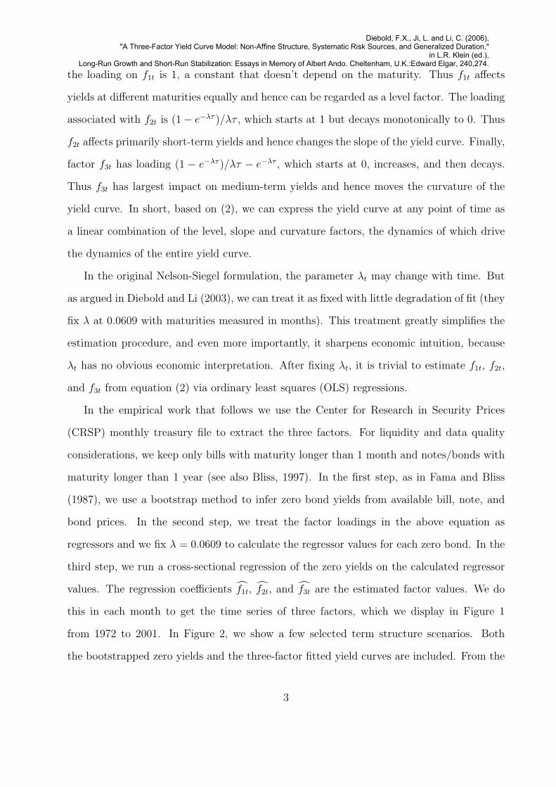
Several important points arise. First, Σ is equal to the identity matrix in the canonical

representation, which significantly simplifies the differential equations (5) and (6). Second,

note that K̃ and θ̃ in (5) and (6) are parameters under the equivalent martingale measure,

while the parameters in the canonical representation are all under the physical measure.

Therefore, we have to convert K̃ and θ̃ to K and θ using the transformations

K̃θ̃ = Kθ −

λ1α1

:

λNαN

K̃ = K +

λ1β′1

:

λNβ′N

, (11)

where λi is the market price of risk for factor i. Finally, the canonical representation puts

several restrictions on the parameters of the model in order to guarantee admissibility2 and

stationarity. As we will see, these restrictions have significant implications for our purposes.

In Table 1, we list all parameter restrictions required by ATSM for various N = 3 subclasses.

To check whether our three-factor model is nested within ATSM, we employ the following

approach. First, without loss of generality we identify (f1t, f2t, f3t) in equation (2) as

Y (t) = (Y1t, Y2t, Y3t) in equation (8), such that the initial conditions are satisfied, and

then we derive the implied functional forms for A(τ) and B(τ) from (2). Next, we insert

these implied expressions into the differential equations (5) and (6), from which we can

derive equalities/inequalities required by these two equations. Finally we compare parameter

2Admissibility means that the specification of the model parameters is such that each element of S(t) inequation (3) is strictly positive over the range of Y .

6



restrictions thus derived with those given in Table 1 to see whether the two sets of restrictions

are consistent. If our restrictions are not consistent with those imposed by ATSM, then our

model is not nested within ATSM. We perform this verification procedure for each three-

factor ATSM sub-class: A0(3), A1(3), A2(3), and A3(3).

Before exploring each sub-class, note that from (2) we have

yt(τ) = f1t + f2t1− e−λτ

λτ+ f3t

(1− e−λτ

λτ− e−λτ

),

and from (8), we have

yt(τ) = −A(τ)

τ+

B1(τ)

τY1(t) +

B2(τ)

τY2(t) +

B3(τ)

τY3(t).

Now we peoceed to identify factor fit with factor Yi(t);hence the A(τ) and B(τ) implied

by (2) are

A(τ) ≡ 0

B1(τ) = τ

B2(τ) =1− e−λτ

λτ

B3(τ) =1− e−λτ

λτ− e−λτ . (12)

Note that A(τ) and B(τ) thus defined satisfy the initial condition (7). At this stage, it

seems that our three-factor model is just a special case of the three-factor ATSM. Inserting

the implied “solutions” (12) into the ODEs (5) and (6), and using the specification (9) and

the transformation (11), we obtain

0 = −(K̃θ̃)′B(τ) +1

2

3∑i=1

Bi(τ)2αi − δ0 (13)

7



1

e−λτ

λτe−λτ

= −K̃ ′B(τ)− 1

2

3∑i=1

Bi(τ)2βi + δy. (14)

We then use the four equations (13) and (14) implied by our 3-factor model to derive

parameter restrictions. We include detailed derivations for the four sub-classes A0(3), A1(3),

A2(3), and A3(3) in the appendix. Our results show that there exists no three-factor ATSM

which can generate our three-factor model of the term structure. This reconciles (1) the

poor forecasting performance recently documented for affine term structure models, and (2)

the good forecasting performance recently documented for the Nelson-Siegel model.

3 Assessing the Three-Factor Model

Diebold and Li (2003) show that the three-factor model (2) performs well in both in-sample

fitting and out-of-sample forecasting. In this section, with an eye toward eventual use of

the three-factor model for bond portfolio risk management, we study its cross-sectional

performance. In particular, we ask whether the three factors represent systematic risk

sources, which are priced in the market. In other words, we ask whether the cross section

of bond returns is explained by the loadings of the various bonds on the three factors, in

a fashion that parallels Ross’s (1976) well-known Arbitrage Pricing Theory (APT) model,

which has been used in equity contexts for many years. Interestingly, the APT has been

applied to fixed income assets by only a few authors, notably Elton, Gruber, and Blake

(1995).

8



3.1 Factor Extraction

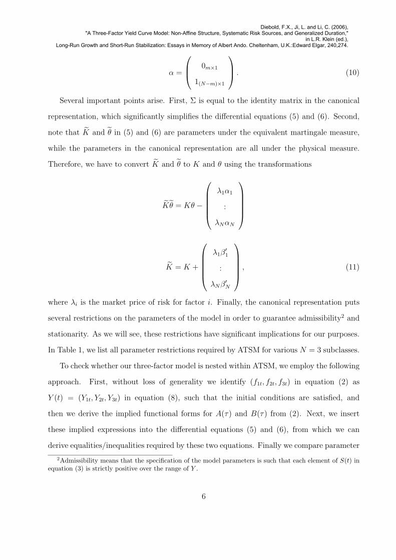
Traditional empirical tests of the APT typically rely on statistical methods, such as principal

components and factor analysis3, to get the factors. For example, Lehmann and Modest

(1988) and Connor and Korajczyk (1988) apply these methods to stocks, while Litterman

and Scheinkman (1991) and Knez, Litterman, and Scheinkman (1994) apply them to bonds.

In particular, Litterman and Scheinkman (1991) and Knez, Litterman, and Scheinkman

(1994) use principal components and factor analysis to extract factors in bond returns. They

conclude that a large portion (up to 98%) of bond return variation can be explained by the

first three principal components or factors. But neither paper considers bond pricing, which

is the focus of this section. In addition, Knez, Litterman, and Scheinkman (1994) consider

only the very short end of yield curve (money market assets). In contrast, we consider the

entire yield curve.

We will compare our three factors with factors extracted from principal components

analysis. We use the CRSP monthly treasury file from Dec. 1971 to Dec 2001. We use the

bootstrapping method outlined in section 2 to infer zero-coupon yields in each time period.

At each t, we consider a set of fixed maturities (measured in months): 3, 6, 9, 12, 15, 18,

21, 24, 30, 36, 48, 60, 72, 84, 96, 108, 120, 168, 180, 192, 216, 240, 264, 288, 312, 336, 360.

These cover the range of bond maturities, and they also reflect the different trading volumes

at different maturities. In particular, at the short end where bonds concentrate, we include

more fixed maturities, and at the long end where there are fewer bonds, we include fewer fixed

maturities. In addition, we cap these fixed maturities with the joint longest maturity within

the time range of interest. For example, from Dec. 1971 to Jan. 1985 with a total of 158

months, we calculate the longest available bond maturities in the market month by month to

get (lt=1, lt=2, ..., lt=158). The minimum of these longest maturities forms the common longest

maturity, and we keep only those fixed maturities smaller than this value in this time range.

We obtain the zero yield at each fixed maturity by reading off or linearly interpolating from

3See also Chen, Roll, and Ross (1986). Elton, Gruber, and Blake (1995), and Ang and Piazzesi (2003).

9



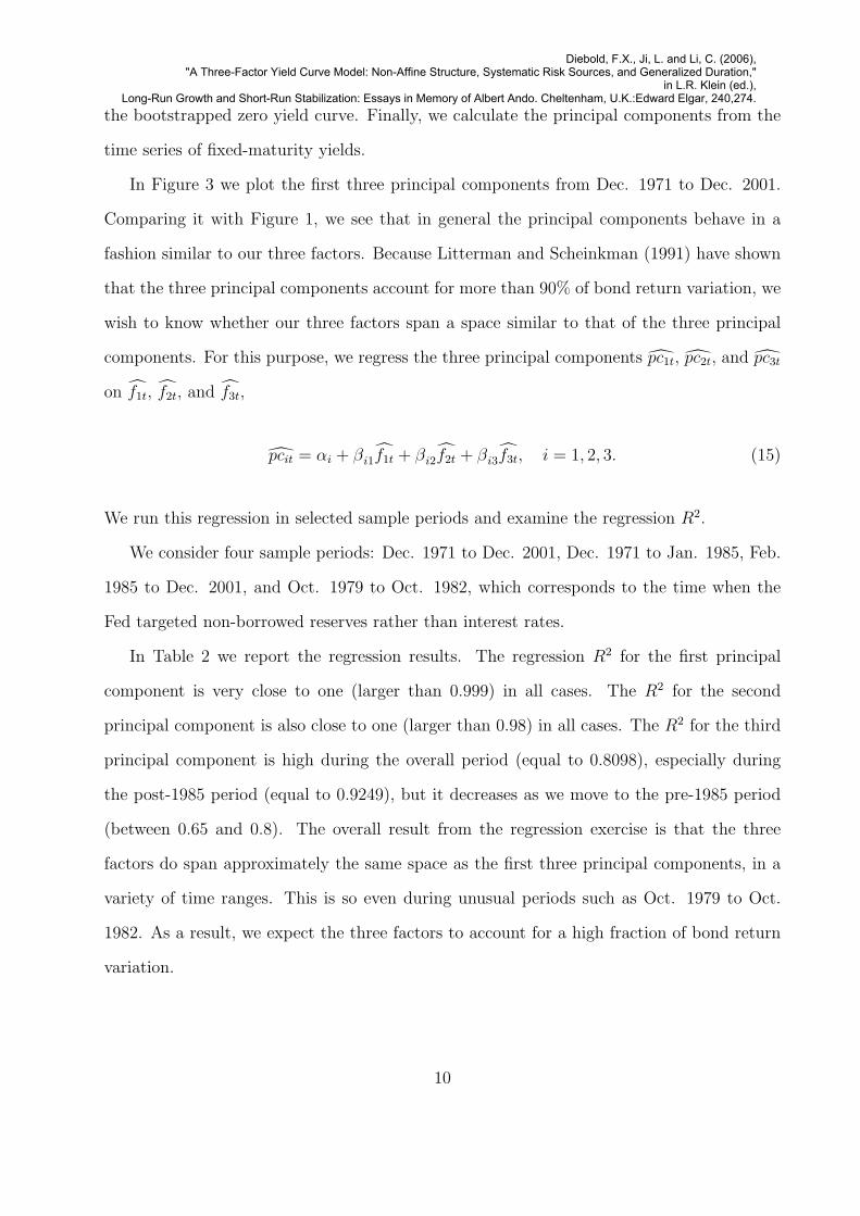
the bootstrapped zero yield curve. Finally, we calculate the principal components from the

time series of fixed-maturity yields.

In Figure 3 we plot the first three principal components from Dec. 1971 to Dec. 2001.

Comparing it with Figure 1, we see that in general the principal components behave in a

fashion similar to our three factors. Because Litterman and Scheinkman (1991) have shown

that the three principal components account for more than 90% of bond return variation, we

wish to know whether our three factors span a space similar to that of the three principal

components. For this purpose, we regress the three principal components p̂c1t, p̂c2t, and p̂c3t

on f̂1t, f̂2t, and f̂3t,

p̂cit = αi + βi1f̂1t + βi2f̂2t + βi3f̂3t, i = 1, 2, 3. (15)

We run this regression in selected sample periods and examine the regression R2.

We consider four sample periods: Dec. 1971 to Dec. 2001, Dec. 1971 to Jan. 1985, Feb.

1985 to Dec. 2001, and Oct. 1979 to Oct. 1982, which corresponds to the time when the

Fed targeted non-borrowed reserves rather than interest rates.

In Table 2 we report the regression results. The regression R2 for the first principal

component is very close to one (larger than 0.999) in all cases. The R2 for the second

principal component is also close to one (larger than 0.98) in all cases. The R2 for the third

principal component is high during the overall period (equal to 0.8098), especially during

the post-1985 period (equal to 0.9249), but it decreases as we move to the pre-1985 period

(between 0.65 and 0.8). The overall result from the regression exercise is that the three

factors do span approximately the same space as the first three principal components, in a

variety of time ranges. This is so even during unusual periods such as Oct. 1979 to Oct.

1982. As a result, we expect the three factors to account for a high fraction of bond return

variation.

10



3.2 An APT Test

Assumptions and procedures for APT tests are well-documented in the literature. We will

follow the usual steps, as for example in Campbell, Lo, and MacKinlay (1997). In particular,

we assume the return generating process,

Rt = a + BFt + εt; E(ε|F ) = 0; E(εε′|F ) = Σ, (16)

where Rt is an N-by-1 vector of returns on the N assets and Ft is a K-by-1 vector of K

factors. We also assume that factors account for the common variation in returns. Under a

no-arbitrage condition, the above structure implies that

µ = `λ0 + BλK , (17)

where µ is an N-by-1 vector of expected returns, ` is a vector of 1’s, B is an N-by-K factor

loading matrix, and λK is a K-by-1 vector of factor risk premia. This is the factor pricing

model we want to estimate and test using maximum likelihood (ML). For that purpose,

we assume returns are dynamically i.i.d. and cross-sectionally jointly normal. We use a

likelihood ratio test statistic, as defined in Campbell, Lo, and MacKinlay(1997),

J = −(T −N/2−K − 1)(log |Σ̂| − log |Σ̂∗|

)∼ χ2(r), (18)

where Σ̂ refers to the ML estimator of the residual covariance without constraints, and Σ̂∗

refers to the ML estimator of the residual covariance with constraints imposed by the pricing

model. Finally, r is the number of restrictions under the null hypothesis.

In our case, the factor pricing model (17) produces the constrained model

Rt = `λ0 + B(λK − E(FKt)) + εt, (19)

11



where the constraint is a = `λ0 + B(λK − E(FKt)). This constraint can be tested using the

J statistic in (18), which in the current context is distributed as χ2(N −K − 1) under the

null that the constraint (and hence the APT) holds.

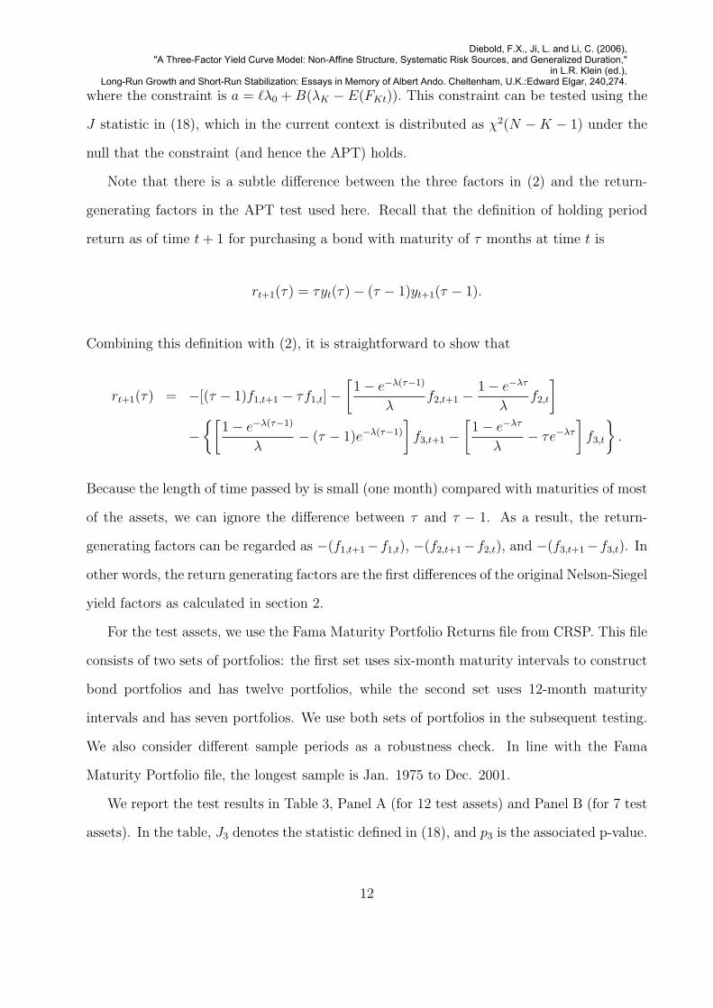
Note that there is a subtle difference between the three factors in (2) and the return-

generating factors in the APT test used here. Recall that the definition of holding period

return as of time t + 1 for purchasing a bond with maturity of τ months at time t is

rt+1(τ) = τyt(τ)− (τ − 1)yt+1(τ − 1).

Combining this definition with (2), it is straightforward to show that

rt+1(τ) = −[(τ − 1)f1,t+1 − τf1,t]−[1− e−λ(τ−1)

λf2,t+1 − 1− e−λτ

λf2,t

]

−{[

1− e−λ(τ−1)

λ− (τ − 1)e−λ(τ−1)

]f3,t+1 −

[1− e−λτ

λ− τe−λτ

]f3,t

}.

Because the length of time passed by is small (one month) compared with maturities of most

of the assets, we can ignore the difference between τ and τ − 1. As a result, the return-

generating factors can be regarded as −(f1,t+1−f1,t), −(f2,t+1−f2,t), and −(f3,t+1−f3,t). In

other words, the return generating factors are the first differences of the original Nelson-Siegel

yield factors as calculated in section 2.

For the test assets, we use the Fama Maturity Portfolio Returns file from CRSP. This file

consists of two sets of portfolios: the first set uses six-month maturity intervals to construct

bond portfolios and has twelve portfolios, while the second set uses 12-month maturity

intervals and has seven portfolios. We use both sets of portfolios in the subsequent testing.

We also consider different sample periods as a robustness check. In line with the Fama

Maturity Portfolio file, the longest sample is Jan. 1975 to Dec. 2001.

We report the test results in Table 3, Panel A (for 12 test assets) and Panel B (for 7 test

assets). In the table, J3 denotes the statistic defined in (18), and p3 is the associated p-value.

12



For most of the sample periods considered, p3 is large enough so that we fail to reject APT

at the 5% significance level. However, in certain sample periods, we get small p3 values.

For example, when we use the entire sample period, the p3 value becomes small. Structural

shifts may be responsible for this result. As argued by Diebold and Li (2003), 1985 is a

potential break point, after which the term structure is more forecastable. Another possible

break point is 1990. Note that when we use twelve test assets, the p3 value during Jan. 1985

to Dec. 1989 is 0.243, but it drops sharply to 0.098 during Jan. 1985 to Dec. 1990. The

same pattern emerges when we use seven test assets: the p3 value drops from 0.281 (from

Jan. 1985 to Dec. 1989) to 0.118 (from Jan. 1985 to Dec. 1990). This pattern suggests that

1990 is possibly a structural break. Because the overall sample includes at least two possible

breaks, it is no surprise that the p3 value is small, as indicated in the table. However, in the

sample periods that exclude the three possible break dates, our three factors price the test

assets well.

Finally, to check whether our model prices bonds well even in unusual market conditions,

we consider the Fed’s monetary experiment of the early 1980’s, the stock market crash of

1987, and the Asian crisis of 1997-1998. To have a sufficient number of data points for a

formal test, we a window of several years around each of the three stress dates: Oct. 1979

to Oct. 1982 for the Fed’s monetary experiment, Jan. 1985 to Dec. 1989 for the 1987 stock

market crash, and Jan. 1996 to Dec. 2001 for the Asian crisis. It is interesting to note that

the three-factor pricing model holds in each of these three sub-periods: p3 is larger than 0.2

in all cases, whether we use twelve test assets or seven test assets. This suggests the validity

of the three-factor model even in extraordinary market conditions.

We also report the J statistics and associated p-values when we use only the first two

factors (J2 and p2) or only the first factor (J1 and p1). Surprisingly, most of the time we

fail to reject the APT when we use only two factors or one factor, perhaps due to low power

of the tests. But to evaluate the relative performance of the 3-factor, 2-factor, and 1-factor

models, we need to consider them together rather than in isolation. Because the models are

13



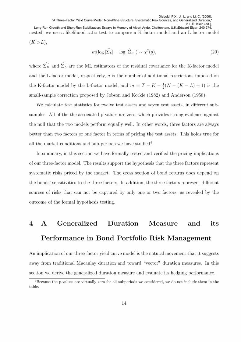
nested, we use a likelihood ratio test to compare a K-factor model and an L-factor model

(K >L),

m(log |Σ̂L| − log |Σ̂K |) ∼ χ2(q), (20)

where Σ̂K and Σ̂L are the ML estimators of the residual covariance for the K-factor model

and the L-factor model, respectively, q is the number of additional restrictions imposed on

the K-factor model by the L-factor model, and m = T − K − 12(N − (K − L) + 1) is the

small-sample correction proposed by Jobson and Korkie (1982) and Anderson (1958).

We calculate test statistics for twelve test assets and seven test assets, in different sub-

samples. All of the the associated p-values are zero, which provides strong evidence against

the null that the two models perform equally well. In other words, three factors are always

better than two factors or one factor in terms of pricing the test assets. This holds true for

all the market conditions and sub-periods we have studied4.

In summary, in this section we have formally tested and verified the pricing implications

of our three-factor model. The results support the hypothesis that the three factors represent

systematic risks priced by the market. The cross section of bond returns does depend on

the bonds’ sensitivities to the three factors. In addition, the three factors represent different

sources of risks that can not be captured by only one or two factors, as revealed by the

outcome of the formal hypothesis testing.

4 A Generalized Duration Measure and its

Performance in Bond Portfolio Risk Management

An implication of our three-factor yield curve model is the natural movement that it suggests

away from traditional Macaulay duration and toward “vector” duration measures. In this

section we derive the generalized duration measure and evaluate its hedging performance.

4Because the p-values are virtually zero for all subperiods we considered, we do not include them in thetable.

14



4.1 Alternative Duration Measures

The concept of duration has a long history in the fixed income literature. Since Macaulay

introduced this concept in 1938, it has been used mostly as a measure of bonds’ sensitivities

to interest rate risk, and it has been widely used in bond portfolio management. But it

was subsequently shown that the Macaulay duration measure works well only when the

yield curve undergoes parallel shifts and when the shifts are small. It breaks down for more

complicated yield curve movements. To overcome this problem, efforts have been made to

extend the duration concept in different directions.

Early work by Cooper (1977), Bierwag (1977), Bierwag and Kaufman (1978), and Khang

(1979) extends the duration measure by presuming various specific characteristic movements

of the term structure. For a brief summary, see Gultekin and Rogalski (1984). Despite the

improvements, the extended duration measures remain one-factor in nature, and as Gultekin

and Rogalski (1984) show, they are very similar. Hence we lump them together and consider

only the Macaulay duration. In another direction, Cox, Ingersoll, and Ross (1985) develop

a general equilibrium model of the term structure, widely known as the CIR model. One

by-product of the model is the stochastic duration measure proposed in Cox, Ingersoll, and

Ross (1979), who argue that the new duration is superior to Macaulay duration and that

the latter overstates the basis risk of bonds.

Other authors are not satisfied with either of these two approaches. They argue that we

need to consider not only movements in the level of the yield curve, but also movements in

other aspects of the curve. That is, we need to use a vector duration whose components

capture different characteristics of movements in the curve. Based on this idea, Chambers,

Carleton, and McEnally (1981) and Garbade (1996) have proposed the use of so-called

duration vectors. Because the elements of their duration vectors derive from polynomial

expansions, we call them polynomial-based duration vectors. However, polynomial-based

duration vectors are unappealing at long maturities, because polynomials diverge at long

maturities, which degrades performance.

15



Motivated by the above considerations, in the next sub-section we take a different

approach to bond portfolio risk management. Our three-factor term structure model

immediately suggests generalized duration components corresponding to the level, slope,

and curvature risk factors. In keeping with the exponential form of the Nelson-Siegel model,

and to distinguish it from the earlier-discussed polynomial model, we call our generalized

duration the exponential-based duration vector, to which we now proceed.

4.2 Generalized Duration

In general we can define a bond duration measure as follows. Let the cash flows from the

bond be C1, C2, ..., CI , and let the associated times to maturity be τ 1,τ 2,...,τ I . Assume also

that the zero yield curve is linear in some arbitrary factors f1, f2, and f3,

yt(τ) = B1(τ)f1t + B2(τ)f2t + B3(τ)f3t (21)

dyt(τ) = B1(τ)df1t + B2(τ)df2t + B3(τ)df3t. (22)

Then, assuming continuous compounding, the price of the bond can be expressed as

P =I∑

i=1

Cie−τ iyt(τ i).

Note that we need to use the corresponding zero yield yt(τ i) to discount cash flow Ci. Then,

for an arbitrary change of the yield curve, the price change is

dP =I∑

i=1

[∂P/∂yt(τ i)] dyt(τ i) =I∑

i=1

[Cie

−τ iyt(τ i)(−τ i)]dyt(τ i),

16



where we have treated yt(τ i) as independent variables. Therefore

−dP

P=

I∑i=1

[1

PCie

−τ iyt(τ i)τ i

]dyt(τ i)

=I∑

i=1

[1

PCie

−τ iyt(τ i)τ i

] 3∑j=1

Bj(τ i)dfjt,

where we have used (21) in the second equality. Now, rearranging terms, we can express the

percentage change in bond price as a function of changes in the factors

−dP

P=

3∑j=1

{I∑

i=1

[1

PCie

−τ iy(τ i)τ i

]Bj(τ i)

}dfjt (23)

=3∑

j=1

{I∑

i=1

wiτ iBj(τ i)

}dfjt,

where wi is the weight associated with Ci.

In (23), we have decomposed the change of bond price into changes in risk factors. Hence

we can define the duration component associated with each risk factor as

Dj =I∑

i=1

wiτ iBj(τ i); j = 1, 2, 3.

In particular, the vector duration based on our three-factor model of yield curve for any

coupon bond is

(D1, D2, D3) =

(I∑

i=1

wiτ i,

I∑i=1

wi1− e−λτ i

λ,

I∑i=1

wi

(1− e−λτ i

λ− τ ie

−λτ i

)). (24)

Although this duration vector has been proposed independently in Willner (1996), our

derivation and discussion are more rigorous, and our subsequent hedging performance

analysis will also be more realistic, using actual bond returns. Note that the first

element of the duration vector is exactly the traditional Macaulay duration, and that it is

straightforward to verify the following additional properties of this vector duration measure:

17



• D1, D2, and D3 move in the same direction, because they are all increasing in τ

• D1, D2, and D3 decrease with coupon rate

• D1, D2, and D3 decrease with yield to maturity

• Portfolio Property: D1, D2, and D3 for a bond portfolio is equal to the average of

individual bonds’ D1, D2, and D3, where the weight assigned to each bond is equal to

the portion of the bond value in the whole portfolio.

As an illustration of how the duration measure changes with coupon rate and time to

maturity, in Figure 4 we plot the three components of the generalized duration measure as

functions of these characteristics (we fix the yield at 5%). The three components increase

with time to maturity and decrease with coupon rate, consistent with our previous conclusion.

As time to maturity increases, D2 and D3 first increase sharply, but they quickly flatten out

around 10 years. By contrast, D1 continues to increase as time to maturity increases. Note

that although D2 and D3 look similar in the plots, they are quite different for maturities up

to 3 years.

In Figure 5, we plot the duration components as functions of coupon rates and yield

to maturity (we fix the time to maturity at 10 years). D1, D2, and D3 all exhibit similar

behavior, decreasing in both coupon rates and yields.

4.3 Comparing Alternative Duration Measures

As discussed above, the performance of our duration measure relative to Macaulay duration,

stochastic duration, and polynomial-based duration will determine its usefulness as a

practical risk management tool.

First, Macaulay duration is simply the first element of our exponential-based duration

vector.

18



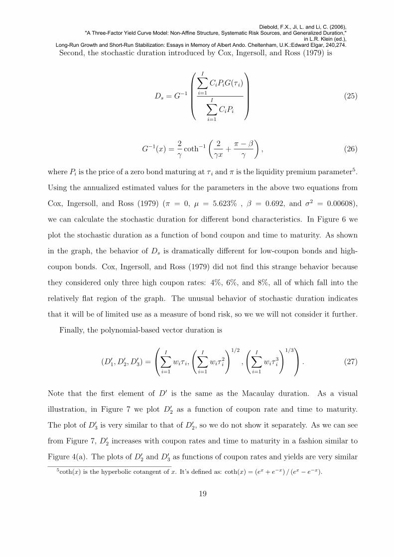
Second, the stochastic duration introduced by Cox, Ingersoll, and Ross (1979) is

Ds = G−1

I∑i=1

CiPiG(τ i)

I∑i=1

CiPi

(25)

G−1(x) =2

γcoth−1

(2

γx+

π − β

γ

), (26)

where Pi is the price of a zero bond maturing at τ i and π is the liquidity premium parameter5.

Using the annualized estimated values for the parameters in the above two equations from

Cox, Ingersoll, and Ross (1979) (π = 0, µ = 5.623% , β = 0.692, and σ2 = 0.00608),

we can calculate the stochastic duration for different bond characteristics. In Figure 6 we

plot the stochastic duration as a function of bond coupon and time to maturity. As shown

in the graph, the behavior of Ds is dramatically different for low-coupon bonds and high-

coupon bonds. Cox, Ingersoll, and Ross (1979) did not find this strange behavior because

they considered only three high coupon rates: 4%, 6%, and 8%, all of which fall into the

relatively flat region of the graph. The unusual behavior of stochastic duration indicates

that it will be of limited use as a measure of bond risk, so we we will not consider it further.

Finally, the polynomial-based vector duration is

(D′1, D

′2, D

′3) =

I∑i=1

wiτ i,

(I∑

i=1

wiτ2i

)1/2

,

(I∑

i=1

wiτ3i

)1/3 . (27)

Note that the first element of D′ is the same as the Macaulay duration. As a visual

illustration, in Figure 7 we plot D′2 as a function of coupon rate and time to maturity.

The plot of D′3 is very similar to that of D′

2, so we do not show it separately. As we can see

from Figure 7, D′2 increases with coupon rates and time to maturity in a fashion similar to

Figure 4(a). The plots of D′2 and D′

3 as functions of coupon rates and yields are very similar

5coth(x) is the hyperbolic cotangent of x. It’s defined as: coth(x) = (ex + e−x) / (ex − e−x).

19



to Figure 5(a), and thus we omit them to save space.

4.4 Risk Management Based on Alternative Duration Measures

Having introduced the definitions and basic properties of Macaulay duration, polynomial-

based vector duration, and exponential-based duration, we apply these measures as

immunization tools in a practical bond portfolio management context. Immunization is

the strategy used to protect the value of the bond portfolio against interest rate changes

by controlling some characteristics of the bond portfolio. In our case, the characteristics for

each duration measure are Macaulay duration Dm, polynomial-based duration D′ = (D′1,

D′2, D

′3), and exponential-based duration D = (D1, D2, D3).

Our empirical immunization design is similar to that in Elton, Gruber, and Nabar (1988).

First we need to specify some bond as the target asset, whose payoffs (returns) we wish to

match (immunize). For each duration measure, we will construct a bond portfolio such

that its duration measure matches that of the target asset. To the extent the duration

measure is a good measure of interest rate risks, the hedging portfolio should have realized

returns approximately equal to those of the target asset. The difference between realized

target returns and realized hedging-portfolio returns (i.e., the hedging errors) will be used

to compare the different duration measures. For a chosen target asset, we can construct

virtually an infinite number of portfolios whose duration matches the target. To narrow

our choice, we use the arguments of Ingersoll (1983) to impose the following minimization

objective

minN∑

n=1

w2n, (28)

subject to two constraints:

(1).N∑

n=1

wn = 1 (29)

20



(2).N∑

n=1

wnDn = Dtarget or

N∑n=1

wnDkn = Dk

target, (30)

where wn is the portfolio weight of bond n, Dn is the duration measure of bond n, and Dtarget

is the duration of the target bond. Note that the second constraint applies to Macaulay

duration and exponential-based vector duration, whereas the third constraint applies to the

polynomial-based duration, because in the latter case the portfolio property applies only to

the moment of the bond, not to the polynomial-based duration per se. Minimizing the sum

of squared weights guarantees diversification of the portfolio. In addition, short sales are

allowed in our design.

We use the CRSP monthly treasury data from Dec. 1971 to Dec. 2001. Because the

three duration measures reduce to the same measure for zero-coupon bonds, we exclude T-

Bills from the immunization universe. As before, for liquidity considerations, we keep only

notes and bonds with maturity longer than one year. But there are still too many bonds

concentrated at the short end. To avoid having too many assets in our portfolio (in any

case, we have at most three duration components to match), we follow Chambers, Carleton,

and McEnally (1988) and consider only government notes maturing on February 15, May

15, August 15, and November 15.

To use the true market price data, our target asset is chosen from existing bonds rather

than an artificially constructed bond as in Willner (1996). We set the target bond’s maturity

at 5 years. At each point of time, it is virtually impossible to find a bond whose time to

maturity is exactly 5 years, so as a compromise we choose as our target asset the bond with

maturity closest to 5 years. We then calculate the duration for the target asset, and we

construct the immunization portfolio from bonds excluding the target bond. In addition,

in portfolio construction, we use only those bonds with return data throughout the holding

period. We solve for the portfolio weights using (28), (29) and (30).

In Table 4 we list the number of assets in the hedging portfolio in different sample periods

and for different holding horizons. In the table, Nmean denotes the average number of assets

21



in the hedging portfolios during that time range. The maximum number of assets goes from

24 to 31, while the minimum number of assets goes from 9 to 22, which suggests that the

number of asets in our hedging portfolio is reasonable. We list in Table 5 the difference

between the target asset’s actual maturity and our ideal target bond maturity, i.e. 5 years.

The average difference Dmean varies from 0.03 year to 0.09 year, a small difference relative

to 5 years. The maximum difference Dmax is 0.37 year, still a reasonably small value.

Once the portfolio is formed, we hold it and the target asset for certain time, which we

set to 1 month, 3 months, 6 months, and 12 months in the current context. We compare the

realized target returns and portfolio returns and record the hedging errors, and we repeat

month-by-month to get the time series of hedging errors.

In Table 6 we list the hedging performance for the three duration measures. In the table,

M refers to hedging using Macaulay duration, E refers to the hedging using exponential-

based duration, and P refers to hedging using polynomial-based duration. As in Chambers,

Carleton, and McEnally (1988), we are mainly interested in the mean absolute hedging error

(MAE) and the standard deviation of the hedging error (Std). The better the hedge, the

smaller these two quantities will be. We also report the mean hedging error. A positive

mean suggests that hedging portfolio is earning a higher average return than the target asset

and is thus a desirable property.

Panel A of Table 6 reveals that, for a 1-month holding period, the exponential-based

duration consistently outperforms Macaulay duration in terms of generating smaller average

absolute hedging error and smaller standard deviation of hedging errors. This is true even

during the pre-1985 period and during the structure-break period of early eighties. In

addition, the average error from exponential-based hedging is consistently larger than that

from the Macaulay hedging. This fact is promising because it implies the exponential-

based hedging can generate higher mean returns while maintaining smaller variation. The

comparison between exponential-based and polynomial-based hedging is less clear-cut. In

most cases they have very similar performance. One exception is the monetary experiment

22



period in the early eighties (10/1979-10/1982). One possible reason is that during that

period the yields were very volatile and noisy as the market were trying to learn the Federal

Reserve’s new policy.

Panel B of Table 6 extends the holding period from one month to one quarter. The

superior performance of exponential-based hedging over Macaulay hedging is again obvious:

we have smaller average absolute error and smaller standard deviation while always keeping

a higher average mean error. Also, this superior performance is more marked than when the

holding period is 1 month. Compared with polynomial-based hedging, exponential-based

hedging still has similar performance. But in the unusual market conditions of the early

eighties, exponential hedging again proves to be superior than polynomial hedging: the

average absolute errors are 0.004 and 0.0044, respectively, and the standard deviations are

0.0049 and 0.0054.

Panels C and D of Table 6 consider even longer holding periods of 6 and 12 months.

The comparative performance of exponential-based hedging vs. Macaulay hedging remains

unchanged: the former is consistently superior to the latter in all samples considered. As

for exponential-based vs. polynomial-based hedging, the results are mixed. On the one

hand, exponential hedging seems to have higher average absolute errors in most cases, but

on the other hand, its hedging errors always have smaller standard deviation. Combining

these two features, it is hard to say which hedging strategy is better. Depending on the

specific needs of the investor, some might prefer exponential-based hedging and others might

prefer polynomial-based hedging. But as before, during the early eighties, exponential-based

hedging proves best: it has the smallest average absolute error and the smallest standard

deviation6.

Overall, Table 6 suggests that hedging based on our vector duration outperforms hedging

based on Macaulay duration in almost all samples and all holding periods. It performs

6Our hedging exercise considers only a single 5 year bond, which has simple cash flows, as the target.For target bonds with more complicated cash flows, say a portfolio of 1 year, 5 year and 10 year bonds, orfor times of high yield level or high volatility, the exponential-based duration might provide a larger hedgingimprovement over the other duration measures.

23



similarly to hedging based on polynomial vector duration in normal times but outperforms

during unusual market situations such as the monetary regime of the early eighties. All told,

our vector duration measure seems to be an appealing risk management instrument for bond

portfolio managers.

5 Conclusion

We have assessed and applied the term-structure model introduced by Nelson and Siegel

(1987) and re-interpreted by Diebold and Li (2003) as a modern three-factor model of level,

slope and curvature. First, we asked whether the model is a member of the affine class,

and we found that it is not. This reconciles (1) the poor forecasting performance recently

documented for affine term structure models, and (2) the good forecasting performance

recently documented for the Nelson-Siegel model. Next, having clarified the relationship

between our three-factor model and the affine class, we proceeded to assess its adequacy

directly, by testing whether its level, slope and curvature factors do indeed capture systematic

risk. We found that they do, and that they are therefore priced. Finally, confident in the

ability of our three-factor model to capture the pricing relations present in the data, we

proceeded to explore its efficacy in bond portfolio risk management, and we found superior

performance relative to hedges constructed using traditional measures such as Macaulay

duration, which account only for level shifts.

Appendix

Here we prove that our three factor model does not belong to ATSM. We will check one-by-

one all four sub-classes of three-factor ATSM: A0(3), A1(3), A2(3), and A3(3).

• A0(3)

24



In this case, the fourth equation from (13) and (14) reduces to

ητe−ητ = −1

ηk33(1− e−ητ ) + k33τe−ητ + δ3 =⇒

0 = −1

ηk33 + δ3 +

1

ηk33e

−ητ + τe−ητ (k33 − η) =⇒

k33 = ηδ3; k33 = 0; k33 = η.

The restrictions on k33 are contradictory. Hence class A0(3) of ATSM is inconsistent with

our three factor model.

• A1(3)

In this case, the first equation from (13) and (14) reduces to

0 = −k11θ1τ − (k21θ1 − λ2 + k31θ1 − λ3)1

η+

1

η2− δ0

+

(k21θ1 − λ2 + k31θ1 − λ3 − 2

η

)1

ηe−ητ

+

(k31θ1 − λ3 − 1

η

)τe−ητ +

1

η2e−2ητ +

1

2τ 2e−2ητ +

1

ητe−2ητ .

This equation requires that k11θ1 = 0, which contradicts the admissibility condition for

A1(3) in Table 1. Therefore, the A1(3) sub-class of ATSM is inconsistent with our three

factor model.

• A2(3)

In this case, the fourth equation in (13) and (14) reduces to

ητe−ητ = −1

ηk33(1− e−ητ ) + k33τe−ητ + δ3 =⇒

0 = −1

ηk33 + δ3 +

1

ηk33e

−ητ + τe−ητ (k33 − η) =⇒

k33 = ηδ3; k33 = 0; k33 = η.

25



Similar to the A0(3) case, the restrictions on A2(3) violates the stationarity condition in

Table 1. Therefore sub-class A2(3) of ATSM is inconsistent with our three factor model.

• A3(3)

In this case, the first equation in (13) and (14) reduces to

0 = (k11θ1 + k12θ2 + k13θ3)τ +1

η(k21θ1 + k22θ2 + k23θ3 + k31θ1 + k32θ2 + k33θ3)

−1

η(k21θ1 + k22θ2 + k23θ3 + k31θ1 + k32θ2 + k33θ3)e

−ητ

−1

η(k31θ1 + k32θ2 + k33θ3)τe−ητ .

This equation alone implies k11θ1 +k12θ2 +k13θ3 = 0 , which contradicts the admissibility

of ATSM in Table 1. Therefore sub-class A3(3) of ATSM is inconsistent with our three factor

model.

26



References

Anderson, T.W., 1958, An Introduction to Multivariate Statistical Analysis, John Wiley andSons, Inc.

Ang, A., and M. Piazzesi, 2003, “A No-Arbitrage Vector Autoregression of TermStructure Dynamics with Macroeconomic and Latent Variables,” Journal of MonetaryEconomics, 50, 4, 745-787.

Bierwag, G.O., 1977, “Immunization, Duration and the Term Structure of Interest Rates,”Journal of Financial and Quantitative Analysis, 12, 725-742.

Bierwag, G.O., and G. Kaufman, 1978, “Bond Portfolio Strategy Simulations: A Critique,”Journal of Financial and Quantitative Analysis, 13, 519-526.

Bliss, R., 1997, “Testing Term Structure Estimation Methods,” Advances in Futures andOptions Research, 9, 197-231.

Bliss, R., and D. Smith, 1997, “The Stability of Interest Rate Processes,” working paper,Federal Reserve Bank of Atlanta.

Campbell, J., A. Lo, and C. MacKinlay, 1997, The Econometrics of Financial Markets,Princeton University Press.

Chambers, D., W. Carleton, and R. McEnally, 1988, “Immunizing Default-Free BondPortfolios with a Duration Vector,” Journal of Financial and Quantitative Analysis,23, 89-104.

Chen, N., R. Roll, and S. Ross, 1986, “Economic Forces and the Stock Market,” Journal ofBusiness, 59, 383-404.

Connor, G., and R. Korajczyk, 1988, “Risk and Return in an Equilibrium APT: Applicationof a New Test Methodology,” Journal of Financial Economics, 21, 255-289.

Cooper, I., 1977, “Asset Values, Interest Rate Changes, and Duration,” Journal of Financialand Quantitative Analysis, 12, 701-724.

Cox, J., J. Ingersoll, and S. Ross, 1979,“Duration and the Measurement of Basis Risk,”Journal of Business, 52, 51-61.

Cox, J., J. Ingersoll, and S. Ross, 1985, “A Theory of the Term Structure of Interest Rates,”Econometrica, 53, 385-408.

Dai, Q., and K. Singleton, 2000, “Specification Analysis of Affine Term Structure Models,”Journal of Finance, 55, 1943-1978.

27



Diebold, F.X., and C. Li, 2003, “Forecasting the Term Structure of Government BondYields,” working paper, University of Pennsylvania.

Duffee, G., 2002, “Term Premia and Interest Rate Forecasts in Affine Models,” Journal ofFinance, 57, 405-443.

Duffie, D., and R. Kan, 1996, “A Yield-Factor Model of Interest Rates,” MathematicalFinance, 6, 379-406.

Elton, E., M. Gruber, and P. Nabar, 1988, “Bond Returns, Immunization and the ReturnGenerating Process,” Studies in Banking and Finance, 5, 125-154.

Elton, E., M. Gruber, and C. Blake, 1995, “Fundamental Economic Variables, ExpectedReturns, and Bond Fund Performance,” Journal of Finance, 50, 1229-1256.

Fama, E., and R. Bliss, 1987, “The Information in Long-Maturity Forward Rates,” AmericanEconomic Review, 77, 680-692.

Garbade, K., 1996, Fixed Income Analytics, MIT Press.

Gultekin, B., and R. Rogalski, 1984, “Alternative Duration Specifications and theMeasurement of Basis Risk: Empirical Tests,” Journal of Business, 57, 241-264.

Ingersoll, J., 1983, “Is Duration Feasible? Evidence from the CRSP Data,” in G.O. Bierwag,G. Kaufman, A. Toves, eds., Innovations in Bond Portfolio Management: DurationAnalysis and Immunization, JAI Press.

Jobson, J.D., and B. Korkie, 1982, “Potential Performance and Tests of Portfolio Efficiency,”Journal of Financial Economics, 10, 433-466.

Khang, C., 1979, “Bond Immunization when Short-Term Rates Fluctuate more than Long-Term Rates,” Journal of Financial and Quantitative Analysis, 13, 1085-1090.

Knez, P., R. Litterman, and J. Scheinkman, 1994, “Explorations into Factors ExplainingMoney Market Returns,” Journal of Finance, 49, 1861-1882.

Lehmann, B., and D. Modest, 1988, “The Empirical Foundations of the Arbitrage PricingTheory,” Journal of Financial Economics, 21, 213-254.

Litterman, R., and J. Scheinkman, 1991, “Common Factors Affecting Bond Returns,”Journal of Fixed Income, June, 54-61.

Nelson, C.R., and A.F. Siegel, “Parsimonious Modeling of Yield Curve,” Journal of Business,60, 473-489.

28



Piazzesi, M., 2002, “Affine Term Structure Models,” working paper, UCLA Anderson Schoolof Management.

Ross, S., 1976, “The Arbitrage Theory of Capital Asset Pricing,” Journal of EconomicTheory, 13, 341-360.

Vasicek, O., 1977, “An Equilibrium Characterization of the Term Structure,” Journal ofFinancial Economics, 5, 177-188.

Willner, R., 1996, “A New Tool For Portfolio Managers: Level, Slope, and CurvatureDurations,” Journal of Fixed Income, June, 48-59.

29



Table 1: Parameter Restrictions for the Three-Factor ATSM

We list parameter restrictions imposed on canonical (maximal) three-factor ATSM models: A0(3),A1(3), A2(3), and A3(3). “eigen” refers to eigenvalues of the corresponding matrix.

Model Existence/Admissibility Stationarity

δ1 ≥ 0 k11 ≥ 0A0(3) δ2 ≥ 0 k22 ≥ 0

δ3 ≥ 0 k33 ≥ 0

δ2 ≥ 0; δ3 ≥ 0 k11 ≥ 0

A1(3) k11θ1 > 0; θ1 ≥ 0 eigen

(k22 k23

k32 k33

)> 0

β12 ≥ 0; β13 ≥ 0

δ3 ≥ 0 k33 ≥ 0k11θ1 + k12θ2 > 0

A2(3) k21θ1 + k22θ2 > 0 eigen

(k11 k12

k21 k22

)> 0

k21 ≤ 0; k12 ≤ 0θ1 ≥ 0; θ2 ≥ 0

k11θ1 + k12θ2 + k13θ3 > 0k21θ1 + k22θ2 + k23θ3 > 0

A3(3) k31θ1 + k32θ2 + k33θ3 > 0 eigen

k11 k12 k13

k21 k22 k23

k31 k32 k33

> 0

k21 ≤ 0; k12 ≤ 0k23 ≤ 0; k32 ≤ 0k13 ≤ 0; k31 ≤ 0

30



Table 2: Regressions of Three Principal Components on the Three Factors

For each sample period, we report the coefficients from regressions of each principal component pci

on a constant and three Nelson-Siegel factors (f1, f2, and f3), with corresponding t statistics inparenthesis. The last column contains the regression R2.

Constant f1 f2 f3 R2

Sample period: 12/1971 - 12/2001

pc1 -0.077 1.008 0.489 0.222 0.9998(-1090.4) (1257.4) (560.8) (267.9)

pc2 -0.143 1.052 -2.917 0.218 0.9885(-94.6) (61.4) (-156.9) (12.3)

pc3 -0.105 1.451 1.022 -3.531 0.8098(-13.4) (16.3) (10.6) (-38.4)

Sample period: 02/1985 - 12/2001

pc1 -0.068 0.992 0.345 0.183 0.9997(-631.8) (643.7) (223.7) (158.3)

pc2 -0.199 0.826 -5.148 -0.959 0.9997(-85.9) (24.9) (-155.2) (-38.7)

pc3 -0.045 0.768 0.942 -0.904 0.9249(-25.9) (30.5) (37.4) (-48.0)

Sample period: 12/1971 - 01/1985

pc1 -0.092 1.009 0.489 0.222 0.9998(-711.7) (764.9) (299.7) (120.5)

pc2 -0.133 0.989 -3.602 0.217 0.9910(-54.1) (39.6) (-116.5) (6.2)

pc3 -0.026 1.407 -2.321 -11.405 0.6464(-0.544) (2.9) (-3.8) (-16.6)

Sample period: 10/1979 - 10/1982

pc1 -0.128 1.000 0.495 0.221 0.9995(-201.6) (193.8) (158.9) (75.7)

pc2 -0.128 1.035 -1.111 0.260 0.9946(-27.9) (27.9) (-49.8) (12.4)

pc3 -0.176 1.582 -0.794 -1.537 0.7946(-5.6) (6.2) (-5.2) (-10.7)

31



Table 3: APT Test of the Three Factor Model

We report APT-J test statistics using different test assets and for different sample periods. TheJ1, J2, J3 columns contain the J-statistics as defined in (18) when we use the first factor, the firsttwo factors, and all three factors, respectively. The p1, p2, p3 columns contain the correspondingp-values. Panel A uses Fama Maturity Portfolios with a 6-month maturity interval as the testassets, while Panel B uses Fama Maturity Portfolios with a 12-month maturity interval as the testassets.

Sample Period J3 p3 J2 p2 J1 p1

Panel A: 6-month maturity interval test assets

01/1975 - 12/2001 28.331 0.001 29.871 0.001 32.590 0.00001/1975 - 12/1984 10.824 0.212 11.508 0.243 12.079 0.27901/1985 - 12/2001 15.879 0.044 22.331 0.008 66.442 0.00001/1985 - 12/1989 10.322 0.243 14.315 0.112 26.088 0.00401/1985 - 12/1990 13.405 0.098 18.215 0.033 33.068 0.00001/1990 - 12/2001 10.064 0.261 13.650 0.135 54.143 0.00010/1979 - 10/1982 6.050 0.642 6.304 0.709 6.670 0.75601/1996 - 12/2001 10.093 0.259 12.741 0.175 27.304 0.002

Panel B: 12-month maturity interval test assets

01/1972 - 12/2001 7.137 0.068 7.230 0.124 10.638 0.05901/1972 - 12/1984 2.259 0.521 2.298 0.681 3.167 0.67401/1985 - 12/2001 5.012 0.171 6.391 0.171 27.164 0.00001/1985 - 12/1989 3.829 0.281 3.919 0.417 5.255 0.38601/1985 - 12/1990 5.865 0.118 6.001 0.199 8.929 0.11201/1990 - 12/2001 2.230 0.526 3.263 0.514 24.532 0.00010/1979 - 10/1982 0.751 0.861 1.134 0.888 1.856 0.86901/1996 - 12/2001 0.750 0.861 1.907 0.753 9.907 0.078

32



Table 4: Number of Assets in the Hedging Portfolios

We report the average (Nmean), maximum (Nmax), and minimum (Nmin) number of assets inhedging (immunization) portfolios for different holding periods and during different sample periods.

Time Nmean Nmax Nmin

1-month holding period

12/1971 - 12/1984 20 29 1201/1985 - 12/2001 28 32 2212/1971 - 12/2001 25 32 12


12/1971 - 12/1984 20 28 1201/1985 - 12/2001 28 31 2112/1971 - 12/2001 24 31 12


12/1971 - 12/1984 18 26 1101/1985 - 12/2001 27 30 2112/1971 - 12/2001 23 30 11


12/1971 - 12/1984 16 24 901/1985 - 12/2001 25 28 2012/1971 - 12/2001 21 28 9

33



Table 5: Divergence Between the Target Asset’s Maturity and the Five-Year Target Maturity

We present the average (Dmean), the maximum (Dmax), and the minimum (Dmin) difference,measured in years, between the empirically chosen target asset’s maturity and our theoretical targetbond maturity of five years.

Time Dmean Dmax Dmin

12/1971 - 12/1984 0.09 0.37 0.0301/1985 - 12/2001 0.03 0.21 012/1971 - 12/2001 0.06 0.37 0

34



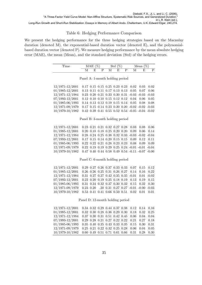
Table 6: Hedging Performance Comparison

We present the hedging performance for the three hedging strategies based on the Macaulayduration (denoted M), the exponential-based duration vector (denoted E), and the polynomial-based duration vector (denoted P). We measure hedging performance by the mean absolute hedgingerror (MAE), the mean (Mean), and the standard deviation (Std) of the hedging errors.

Time MAE (%) Std (%) Mean (%)M E P M E P M E P

Panel A: 1-month holding period

12/1971-12/2001 0.17 0.15 0.15 0.25 0.23 0.23 0.02 0.03 0.0201/1985-12/2001 0.13 0.11 0.11 0.17 0.13 0.13 0.05 0.07 0.0612/1971-12/1984 0.23 0.20 0.21 0.33 0.30 0.31 -0.03 -0.03 -0.0307/1993-12/2001 0.12 0.10 0.10 0.15 0.12 0.12 0.04 0.06 0.0501/1985-06/1993 0.14 0.13 0.12 0.19 0.15 0.14 0.05 0.08 0.0812/1971-09/1979 0.17 0.15 0.14 0.23 0.20 0.20 -0.02 -0.02 -0.0310/1979-10/1982 0.42 0.39 0.41 0.55 0.52 0.54 -0.05 -0.04 -0.02

Panel B: 3-month holding period

12/1971-12/2001 0.23 0.21 0.21 0.32 0.27 0.28 0.03 0.08 0.0601/1985-12/2001 0.20 0.18 0.18 0.25 0.20 0.20 0.09 0.06 0.1412/1971-12/1984 0.28 0.24 0.25 0.38 0.32 0.33 -0.03 -0.02 -0.0407/1993-12/2001 0.17 0.15 0.14 0.20 0.15 0.15 0.09 0.12 0.1101/1985-06/1993 0.22 0.22 0.21 0.28 0.23 0.23 0.08 0.09 0.0912/1971-09/1979 0.22 0.19 0.19 0.29 0.25 0.24 -0.01 -0.01 -0.0410/1979-10/1982 0.47 0.40 0.44 0.58 0.49 0.54 -0.11 -0.07 -0.06

Panel C: 6-month holding period

12/1971-12/2001 0.29 0.27 0.26 0.37 0.33 0.33 0.07 0.15 0.1201/1985-12/2001 0.26 0.26 0.25 0.31 0.26 0.27 0.14 0.16 0.2212/1971-12/1984 0.31 0.27 0.27 0.42 0.35 0.35 -0.01 0.01 -0.0207/1993-12/2001 0.22 0.20 0.19 0.25 0.18 0.19 0.13 0.19 0.1501/1985-06/1993 0.31 0.34 0.32 0.37 0.30 0.32 0.15 0.32 0.3012/1971-09/1979 0.23 0.20 .20 0.31 0.27 0.27 -0.01 -0.00 -0.0310/1979-10/1982 0.53 0.41 0.41 0.66 0.50 0.51 0.02 0.01 0.01

Panel D: 12-month holding period

12/1971-12/2001 0.34 0.32 0.29 0.44 0.37 0.38 0.12 0.14 0.1601/1985-12/2001 0.32 0.30 0.28 0.36 0.29 0.30 0.18 0.32 0.2512/1971-12/1984 0.37 0.30 0.31 0.51 0.42 0.45 0.06 0.04 0.0407/1993-12/2001 0.29 0.28 0.21 0.27 0.22 0.22 0.21 0.27 0.1801/1985-06/1993 0.35 0.40 0.35 0.43 0.33 0.35 0.15 0.30 0.3112/1971-09/1979 0.25 0.21 0.22 0.32 0.25 0.28 0.06 0.04 0.0510/1979-10/1982 0.60 0.49 0.51 0.71 0.61 0.66 0.31 0.28 0.30

35



Figure 1: Time Series Plot of the Three Factors

We present the time series of the level, slope, and curvature factors. We extract these factors fromzero-coupon bond yields using OLS regressions of (2) with λ fixed at 0.0609.

Jan70 Jan75 Jan80 Jan85 Jan90 Jan95 Jan00 Jan050.05

0.1

0.15

0.2

fact

or v

alue

factor 1

Jan70 Jan75 Jan80 Jan85 Jan90 Jan95 Jan00 Jan05−0.1

−0.05

0

0.05

0.1

fact

or v

alue

factor 2


−0.05

0

0.05

0.1

fact

or v

alue

factor 3

36



Figure 2: Selected Model-Based Yield Curves

We plot bootstrapped raw zero yields and model-implied zero yields on the following days:02/28/1997, 04/30/1974, 09/30/1981, and 12/29/2000. We select these days to represent differentyield curve shapes: increasing, decreasing, humped, and inverted humped.

0 50 100 150 200 250 300 350 4000.05

0.055

0.06

0.065

0.07

0.075

0.08Yield Curve on 02/28/1997

yiel

d

maturities (months)

0 50 100 150 200 2500.065

0.07

0.075

0.08

0.085

0.09


yiel

d

maturities (months)

0 50 100 150 200 2500.14

0.145

0.15

0.155

0.16

0.165


yiel

d

maturities (months)

0 50 100 150 200 250 300 3500.05

0.052

0.054

0.056

0.058

0.06


yiel

d

maturities (months)

37



Figure 3: Time Series Plot of First Three Principal Components

We present the time series of the first three principal components extracted from fixed-maturityzero-coupon bond yields inferred from all bond data. We choose these fixed maturities so that yielddata exist throughout Dec 1971 to Dec 2001.


0

0.05

0.1

0.15

valu

e

component 1


−0.1

0

0.1

0.2

valu

e

component 2


−0.2

0

0.2

0.4

valu

e

component 3

38



Figure 4: Exponential-Based Duration Vector

We plot the three elements of the exponential-based duration vector D, defined in equation (24),as a function of coupon rates and time to maturity. The first element is the Macaulay duration.We fix the bond yield at 5%.

0

100

200

300

400

0

0.05

0.1

0.15

0.20

5

10

15

20

25

30

35

Maturity (months)

D1 as a function of Coupon and Maturity

Coupon Rate

D1 (

year

s)

(a)

0

100

200

300

400

0

0.05

0.1

0.15

0.20

0.2

0.4

0.6

0.8

1

1.2

1.4

Maturity (months)


Coupon Rate

D2 (

year

s)

(b)

0

100

200

300

400

0

0.05

0.1

0.15

0.20

0.2

0.4

0.6

0.8

1

1.2

1.4

Maturity (months)


Coupon Rate

D3 (

year

s)

(c)

39



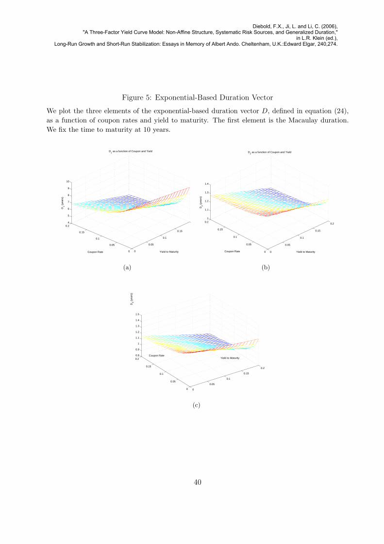
Figure 5: Exponential-Based Duration Vector

We plot the three elements of the exponential-based duration vector D, defined in equation (24),as a function of coupon rates and yield to maturity. The first element is the Macaulay duration.We fix the time to maturity at 10 years.

0

0.05

0.1

0.15

0.2

0

0.05

0.1

0.15

0.24

5

6

7

8

9

10

Yield to Maturity

D1 as a function of Coupon and Yield

Coupon Rate

D1 (

year

s)

(a)

0

0.05

0.1

0.15

0.2

0

0.05

0.1

0.15

0.21

1.1

1.2

1.3

1.4

Yield to Maturity

D2 as a function of Coupon and Yield

Coupon Rate

D2 (

year

s)

(b)

0

0.05

0.1

0.15

0.2

0

0.05

0.1

0.15

0.20.8

0.9

1

1.1

1.2

1.3

1.4

1.5

Yield to MaturityCoupon Rate

D3 (

year

s)

(c)

40



Figure 6: Stochastic Duration

We plot the stochastic duration Ds, defined in equations (25) and (26), as a function of couponrates and time to maturity. We fix the bond yield at 5% and use the following parameter values:π = 0, µ = 5.623%, β = 0.692, and σ2 = 0.00608.

0

100

200

300

400

0

0.05

0.1

0.15

0.20

5

10

15

20

25

30

35

Maturity (months)Coupon Rate

Ds’

(ye

ars)

41



Figure 7: Second Element of the Polynomial-Based Duration Vector

We plot the second element of polynomial-based duration vector D′2, defined in equation (27), as a

function of coupon rates and time to maturity. We fix the bond yield at 5%.

0

100

200

300

400

0

0.05

0.1

0.15

0.20

5

10

15

20

25

30

35

Maturity (months)Coupon Rate

D2’ (

year

s)

42



Documents

A Three-Factor Yield Curve Model: Non-A–ne Structure, …fdiebold/papers/paper60/djl.pdf · Non-A–ne Structure, Systematic Risk Sources, and ... Systematic Risk Sources, and Generalized