www.actamat-journals.com

Acta Materialia 54 (2006) 3953–3960

A thick-interface model for diffusive and massive phasetransformation in substitutional alloys

J. Svoboda a,*, J. Vala b, E. Gamsjager c, F.D. Fischer c

a Institute of Physics of Materials, Academy of Sciences of the Czech Republic, Zizkova 22, CZ-61662 Brno, Czech Republicb Faculty of Civil Engineering, Brno University of Technology, Zizkova 17, CZ-60200 Brno, Czech Republic

c Institute of Mechanics, Montanuniversitat Leoben, Franz-Josef-Straße 18, A-8700 Leoben, Austria

Received 24 February 2006; received in revised form 20 April 2006; accepted 22 April 2006Available online 7 July 2006

Abstract

Based on the application of the thermodynamic extremal principle, a new model for the diffusive and massive phase transformationin multicomponent substitutional alloys is developed. Interfacial reactions such as the rearrangement of the lattice, solute drag and trans-interface diffusion are automatically considered by assigning a finite thickness and a finite mobility to the interface region. As an appli-cation of the steady-state solution of the derived evolution equations, the kinetics of the massive c! a transformation in the Fe-richFe–Cr–Ni system is simulated. The thermodynamic properties of the interface may influence significantly the contact conditions atthe interface as well as the conditions for the occurrence of the massive transformation and its kinetics. The model is also used forthe simulation of the diffusion-induced grain boundary migration in the same system. By application of the model a realistic valuefor the Gibbs energy per unit interface area is obtained.� 2006 Acta Materialia Inc. Published by Elsevier Ltd. All rights reserved.

Keywords: Phase transformation; Diffusion; Modelling; Interface kinetics; Diffusion-induced grain boundary migration

1. Introduction

To simulate diffusional phase transformations, it is nec-essary to solve the coupled problem of diffusion and inter-face migration. Usually, the interface is assumed to besharp, and ortho-equilibrium (continuous chemical poten-tials of all components across the interface) or para-equilib-rium (continuous chemical potentials of interstitialcomponents and continuous site fractions of substitutionalcomponents across the interface) contact conditions areapplied at the interface. A more general set of contact con-ditions at a sharp interface with a finite mobility restrictsthe continuity in chemical potentials to the interstitial ele-ments only and allows identical jumps in chemical poten-tials for all substitutional elements [1]. In the case ofsubstitutional alloys, assuming a sharp migrating interface

1359-6454/$30.00 � 2006 Acta Materialia Inc. Published by Elsevier Ltd. All

doi:10.1016/j.actamat.2006.04.027

* Corresponding author. Tel.: + 420 5 412 18657.E-mail address: svobj@ipm.cz (J. Svoboda).

of finite mobility, the contact condition represented byidentical jumps of the chemical potentials of the substitu-tional elements is also derived by application of the ther-modynamic extremal principle [2].

A real migrating interface of finite thickness h may,however, drag segregated impurity atoms forming concen-tration profiles across the interface. Such a local diffusionprocess may reduce the migration velocity v of the interfacedue to the Gibbs energy dissipated by this local diffusionprocess. This decelerating effect is called solute drag. Prom-inent approaches by Lucke and Stuwe [3] and Cahn et al.[4] are reported in the literature – for other references seee.g. Ref. [5]. In contrast to the results of the classic workson solute drag, Svoboda et al. [5] allow differences of thechemical potential for the solvent as well as for the intersti-tial solute component in binary systems. The diffusion ofthe solute across the interface is driven by the gradient ofthe chemical potential of the solute, and the interfacemigration is driven by the difference of the chemical

rights reserved.

3954 J. Svoboda et al. / Acta Materialia 54 (2006) 3953–3960

potential of the solvent across the interface (a finite inter-face mobility is supposed). A similar approach, based onthe balance for the total Gibbs energy in the interface,was later used by Odquist et al. [6] for multicomponentsystems.

The solute drag effect does not only lead to the occur-rence of jumps of the chemical potentials of interstitial ele-ments segregating in the interface, but may also changesignificantly the jumps of the chemical potentials of substi-tutional components, which eventually breaks the condi-tion to be identical for all substitutional components aspredicted in Refs. [1,2]. As a consequence this may leadto a situation in which the massive transformation mayoccur in the two-phase region as has been experimentallyproven for several systems (e.g. Ref. [7]) and discussed indetail in Ref. [8].

The goal of this paper is to present a thick-interfacemodel for the diffusive transformation in multicomponentsystems consisting of substitutional components that isbased on the application of the thermodynamic extremalprinciple (e.g. see Refs. [2,9,10]). The model takes intoaccount solute drag and trans-interface diffusion as wellas a finite interface mobility. The steady-state solution ofthe derived equations is then applied to the Fe-rich Fe–Cr–Ni system to simulate the massive c! a transforma-tion. The influence of thermodynamic properties of theinterface on kinetics and conditions for the massive trans-formation are discussed in detail. The model is also usedfor simulation of the diffusion-induced grain boundarymigration (DIGM) in the same system.

2. The model

A one-dimensional, two-phase system of unit cross-sec-tional area with r substitutional components is considered,in which the c! a transformation occurs (see Fig. 1). Thelocal chemical composition is described by mole fractions~x ¼ ðx1ðz; tÞ; . . . ; xr�1ðz; tÞÞ, with z being the coordinateand t being the time. The mole fraction of the componentr is given by

xrðz; tÞ ¼ 1�Xr�1

k¼1

xkðz; tÞ: ð1Þ

Fig. 1. System geometry.

The system moves with the velocity v(t), being the velocityof interface migration to the left, relative to a fixed coordi-nate system. Thus, the position of the interface is fixed inthe coordinate system, and one can choose the origin ofthe coordinate system to coincide with the left-hand surfaceof the interface of thickness h (see Fig. 1). The left and rightends of the system have the coordinates zL and zR, respec-tively, both of which depend on time. Furthermore, weassume that non-zero diffusive fluxes ja�

k and jc�k can be im-

posed at both ends of the specimen.Let a be a scalar quantity a = a(z, t). Then its material

(or total time) derivative in the actual configuration con-nected with the moving system _a ¼ da=dt and the partialtime derivative oa/ot are related by

_a ¼ oaot� v

oaoz: ð2Þ

Furthermore, the time derivative of an integral quantity isgiven by

d

dt

Z zR

zL

a dz ¼Z zR

zL

_adz: ð3Þ

if ddt ðdzÞ ¼ 0 is assumed (see Section 2.1 of Ref. [11]). The

chemical potential lk of component k is supposed to be afunction of ~x and of z. The dependence on z determinesto which phase or to which position in the interface thematerial point belongs. Consequently, as ~x is a functionof z and t, we can formally write lk as a certain functionof z and t.

We suppose that the dependencies of the chemicalpotentials on ~x are known for both the a and c phases aswell as for the interface I between both phases supposedto be a third phase denoted by b (see Fig. 1); i.e. la

kð~xÞ,lb

k ð~xÞ and lckð~xÞ are known functions. For the chemical

potentials of phases a, b or c the well-known Gibbs–Duhem relation (see Appendix in Ref. [12] for details)holdsXr

k¼1

xk dlfk ¼

Xr

k¼1

xkolf

k

ozdzþ olf

k

otdt

!¼ 0: ð4Þ

where f represents the phase a, b or c. If we choose dt = 0,the Gibbs–Duhem relation readsXr

k¼1

xkolf

k

oz¼ 0: ð5Þ

Dividing Eq. (4) by the time increment dt yieldsXr

k¼1

xk _lfk ¼ 0: ð6Þ

Alternatively Eq. (6) can be obtained using dz = �vdt andEq. (2).

The chemical potential lk can be calculated at any pointof the specimen as

lkðz;~xÞ ¼X

f2fa;b;cgwf ðzÞlf

k ð~xÞ: ð7Þ

J. Svoboda et al. / Acta Materialia 54 (2006) 3953–3960 3955

The functions wf(z) are supposed to be reasonably contin-uous weight functions, having the properties

waðzÞ ¼ 1 for z 6 0; waðzÞ ¼ 0 for z P h=2;

wcðzÞ ¼ 0 for z 6 h=2; wcðzÞ ¼ 1 for z P h: ð8Þ

and wb(z) = 1 � wa(z) � wc(z) for every z between zL andzR. Note that the Gibbs–Duhem Eqs. (5) and (6) for lk in-stead of lf

k are not fulfilled in the region 0 6 z 6 h (in theinterface I).

For the application of the thermodynamic extremalprinciple, it is necessary to calculate the rate _G of the totalGibbs energy G of the system and the total dissipation Q inthe system.

2.1. Total Gibbs energy and its rate

The total Gibbs energy G of the system is given by

G ¼ 1

X

Xr

k¼1

Z zR

zL

xklk dz; ð9Þ

where X is the molar volume. By assuming that the im-posed fluxes ja�

k � jkðzLÞ and jc�k � jkðzRÞ (see Fig. 1) are

zero, the time derivative of G can be calculated using Eq.(3) as

_G ¼ 1

X

Xr

k¼1

Z zR

zL

ð _xklk þ xk _lkÞdz: ð10Þ

Using Eqs. (2), (7) and (8) together with the Gibbs–Duhemrelation in the form of Eq. (4), one gets

_G ¼ 1

X

Xr

k¼1

Z zR

zL

_xklk dz� vX

f2fa;b;cg

Z h

0

xkdwf

dzlf

k dz

!:

ð11ÞAccording to the Gibbs–Duhem relation in the form of Eq.(5) and using Eq. (7), Eq. (11) can be rewritten as

_G ¼ 1

X

Xr

k¼1

Z zR

zL

_xklk dz� vZ h

0

xkolk

ozdz

� �: ð12Þ

The mass conservation law for the component k with thediffusive flux jk reads

_xk ¼ �Xojk

oz: ð13Þ

Insertion of Eq. (13) into Eq. (12) and integration of thefirst term in Eq. (12) by parts yield

_G ¼Xr

k¼1

Z zR

zL

jk

olk

ozdz� 1

XvZ h

0

xkolk

ozdz: ð14Þ

2.2. Rate of the total Gibbs energy dissipation

The rate of the total Gibbs energy dissipation due tobulk diffusion and interface migration is given by [2,10]

Q ¼Xr

k¼1

Z zR

zL

j2k

Akdzþ v2

M; Ak ¼

xkDk

XRT: ð15Þ

The quantity Dk is the tracer diffusion coefficient of compo-nent k, R is the gas constant, T is the absolute temperatureand M is the interface mobility.

We assume negligible vacancy fluxes in the system,which together with the vacancy mechanism of diffusionleads to the constraintXr

k¼1

jk � 0: ð16Þ

Using Eqs. (13) and (16) leads toXr

k¼1

_xk ¼ 0: ð17Þ

Thus Eq. (1) is automatically fulfilled during the whole sys-tem evolution, if the starting conditions obey Eq. (1). Theconstraint of Eq. (16) can be taken into account in the for-mulation of the thermodynamic extremal principle bymeans of the Lagrange multiplier method.

2.3. Application of the thermodynamic extremal principle

We use the principle of maximum dissipation rate as itwas first applied by Onsager [9] in 1945 for a diffusionalprocess. According to this thermodynamic extremal princi-ple the kinetics of the system corresponds to the variation[10]

d _Gþ Q2þZ zR

zL

kXr

k¼1

jk dz

!ðj1; . . . ; jr; vÞ ¼ 0: ð18Þ

where k is the Lagrange multiplier to meet Eq. (16).Performing the variations

d _GþQ2þZ zR

zL

kXr

k¼1

jk dz

!ð~j1; . . . ;~jrÞ

¼Xr

k¼1

Z zR

zL

ejkolk

ozdzþ

Xr

k¼1

Z zR

zL

jkejk

Akdzþ

Xr

k¼1

Z zR

zL

~jkkdz¼ 0;

d _GþQ2þZ zR

zL

kXr

k¼1

jk dz

!ðevÞ

¼ � evX

Xr

k¼1

Z h

0

xkolk

ozdzþ vev

M¼ 0; ð19Þ

we obtain for k = 1,. . ., r

olk

ozþ jk

Akþ k ¼ 0 ð20Þ

and

v ¼ MX

Xr

k¼1

Z h

0

xkolk

ozdz: ð21Þ

Multiplication of Eqs. (20) by Ak, their summation andapplication of Eq. (17) allow one to calculate k as

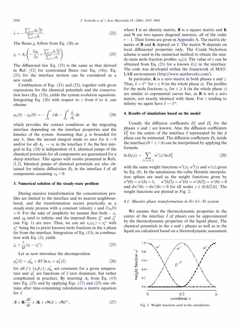
Fig. 2. Weight functions used in the calculations.

3956 J. Svoboda et al. / Acta Materialia 54 (2006) 3953–3960

k ¼ �Pr

k¼1AkolkozPr

l¼1Al: ð22Þ

The fluxes jk follow from Eq. (20) as

jk ¼ Ak �olk

ozþPr

i¼1AioliozPr

l¼1Al

!: ð23Þ

The diffusional law Eq. (23) is the same as that derivedin Ref. [12] for constrained fluxes (see Eq. (16)). Eq.(21) for the interface motion can be considered as anew result.

Combination of Eqs. (21) and (23), together with givenexpressions for the chemical potentials and the conserva-tion laws (Eq. (13)), yields the system evolution equations.Integrating Eq. (20) with respect to z from 0 to h, oneobtains

lkðhÞ � lkð0Þ ¼ �Z h

0

kdz�Z h

0

jk

Akdz: ð24Þ

which provides the contact conditions at the migratinginterface depending on the interface properties and thekinetics of the system. Assuming that jk is bounded forany k, then the second integral tends to zero for h! 0and/or for all Ak !1 in the interface I. As the first inte-gral in Eq. (24) is independent of k, identical jumps of thechemical potentials for all components are guaranteed for asharp interface. This agrees with results presented in Refs.[1,2]. Identical jumps of chemical potentials are also ob-tained for infinite diffusivities Dk in the interface I of allcomponents assuming xk > 0.

3. Numerical solution of the steady-state problem

During massive transformation the concentration pro-files are limited to the interface and its nearest neighbour-hood, and the transformation occurs practically as asteady-state process with a constant velocity v and oxk/ot

= 0. For the sake of simplicity we assume that both – zL

and zR tend to infinity and the imposed fluxes ja�k and jc�

k

(see Fig. 1) are zero. Thus, we can set xkðzLÞ ¼ x1k withx1k being the (a priori known) mole fractions in the a phasefar from the interface. Integration of Eq. (13), in combina-tion with Eq. (2), yields

jk ¼vXðxk � x1k Þ: ð25Þ

Let us now introduce the decomposition

lfk ð~xÞ ¼ lf

0k þ RT ln xk þ ufk ð~xÞ: ð26Þ

for all f 2 {a,b,c}; lf0k are constants for a given tempera-

ture and ufk are functions of ~x (not dominant, but rather

complicated in practice). By inserting Ak from Eq. (15)into Eq. (23) and by applying Eqs. (17) and (25) one ob-tains after time-consuming calculations a matrix equationfor ~x

ðIþ BÞ d~xþ ðKþ vNÞ~x ¼ vN~x1; ð27Þ

dz

where I is an identity matrix, B is a square matrix and K

and N are two square diagonal matrices, all of the orderr � 1. Their forms are given in Appendix A. The matrix ele-ments of B and K depend on~x. The matrix N depends onlocal diffusional properties only. The Crank–Nicholsonscheme is used in the numerical method to obtain the stea-dy-state mole fraction profiles xk(z). The value of v can beobtained from Eq. (21) for a known ~xðzÞ in the interface.The code was developed within the framework of MAT-LAB environment (http://www.mathworks.com/).

In particular, K is a zero matrix in both phases a and c.Thus,~x ¼~x1 for z 6 0 (in the whole phase a). The profilesfor the mole fractions xk for z P h (in the whole phase c)are similar to exponential curves but, as B is not a zeromatrix, not exactly identical with them. For z tending toinfinity we again have~x!~x1.

4. Results of simulations based on the model

Usually the diffusion coefficients Dak and Dc

k for thephases a and c are known. Also the diffusion coefficientsDb

k for the centre of the interface I represented by the bphase can be estimated. The diffusion coefficients Dk insidethe interface (0 < z < h) can be interpolated by applying theformula

ln DkðzÞ ¼X

f2fa;b;cgwf ðzÞ ln Df

k ð28Þ

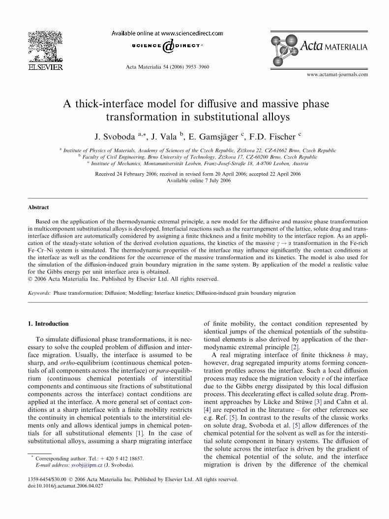
with the same weight functions wa(z), wb(z) and wc(z) givenby Eq. (8). In the simulations the cubic Hermite interpola-tion splines are used as the weight functions given bywa(0) = wc(h) = 1, wa(h/2) = wa(h) = wc(h/2) = wc(0) = 0and dwa/dz = dwc/dz = 0 for all nodes z 2 {0,h/2,h}. Theweight functions are plotted in Fig. 2.

4.1. Massive phase transformation in Fe–Cr–Ni system

We assume that the thermodynamic properties in thecentre of the interface I (b phase) can be approximatedby the thermodynamic properties of the liquid phase. Thechemical potentials in the a and c phases as well as in theliquid are calculated based on a thermodynamic assessment

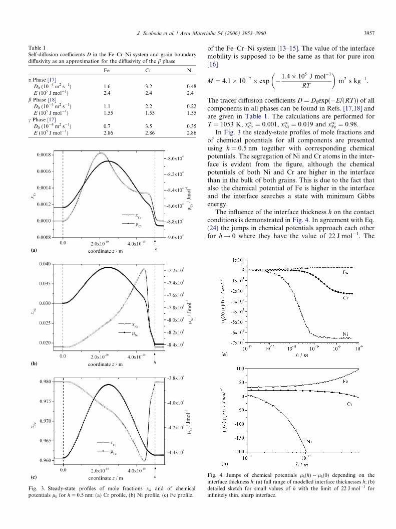
Table 1Self-diffusion coefficients D in the Fe–Cr–Ni system and grain boundarydiffusivity as an approximation for the diffusivity of the b phase

Fe Cr Ni

a Phase [17]D0 (10�4 m2 s�1) 1.6 3.2 0.48E (105 J mol�1) 2.4 2.4 2.4

b Phase [18]D0 (10�4 m2 s�1) 1.1 2.2 0.22E (105 J mol�1) 1.55 1.55 1.55

c Phase [17]D0 (10�4 m2 s�1) 0.7 3.5 0.35E (105 J mol�1) 2.86 2.86 2.86

Fig. 3. Steady-state profiles of mole fractions xk and of chemicalpotentials lk for h = 0.5 nm: (a) Cr profile, (b) Ni profile, (c) Fe profile.

J. Svoboda et al. / Acta Materialia 54 (2006) 3953–3960 3957

of the Fe–Cr–Ni system [13–15]. The value of the interfacemobility is supposed to be the same as that for pure iron[16]

M ¼ 4:1� 10�7 � exp � 1:4� 105 J mol�1

RT

� �m2 s kg�1:

The tracer diffusion coefficients D = D0exp(�E/(RT)) of allcomponents in all phases can be found in Refs. [17,18] andare given in Table 1. The calculations are performed forT = 1053 K, x1Cr ¼ 0:001, x1Ni ¼ 0:019 and x1Fe ¼ 0:98.

In Fig. 3 the steady-state profiles of mole fractions andof chemical potentials for all components are presentedusing h = 0.5 nm together with corresponding chemicalpotentials. The segregation of Ni and Cr atoms in the inter-face is evident from the figure, although the chemicalpotentials of both Ni and Cr are higher in the interfacethan in the bulk of both grains. This is due to the fact thatalso the chemical potential of Fe is higher in the interfaceand the interface searches a state with minimum Gibbsenergy.

The influence of the interface thickness h on the contactconditions is demonstrated in Fig. 4. In agreement with Eq.(24) the jumps in chemical potentials approach each otherfor h! 0 where they have the value of 22 J mol�1. The

Fig. 4. Jumps of chemical potentials lk(h) � lk(0) depending on theinterface thickness h: (a) full range of modelled interface thicknesses h; (b)detailed sketch for small values of h with the limit of 22 J mol�1 forinfinitely thin, sharp interface.

Fig. 6. Calculated and fitted dependences of the grain boundary velocity v

on the values of imposed fluxes j�Cr and j�Ni. Asterisks, calculated values ofv; dashed lines, linear fit; solid line, quadratic fit.

Fig. 5. Temperature dependence of the interface velocity v for differentvalues of the interface thickness h.

Fig. 7. Steady-state profiles of mole fractions xk in the grain boundary inthe austenite at the temperature T = 1070 K for h = 0.5 nm and differentfluxes j�Cr and j�Ni: (a) Cr profiles, (b) Ni profiles.

3958 J. Svoboda et al. / Acta Materialia 54 (2006) 3953–3960

temperature dependence of the steady-state interface veloc-ity v is calculated for various values of interface thickness h

(including h = 0.5 nm from above) and is plotted in Fig. 5.The figure clearly demonstrates a significant influence ofthe interface thickness on the transformation kinetics aswell as on the region of conditions for the massive transfor-mation (region of temperatures with v > 0).

4.2. DIGM in the Fe–Cr–Ni system

The present model can also be used for the simulation ofthe DIGM. In the case that a and c represent identicalphases, the interface represents a grain boundary. Similarlyto the procedure presented in Section 3 one can find thestationary solution of the problem with imposed fluxesja�

i (see Fig. 1). The values of the diffusive fluxes at theleft-hand side of the interface (h = 0), j�i , due to imposedfluxes ja�

i are considered as external parameters, whichcan be changed. Then the application of the stationary con-dition leads again to Eq. (25) and the numerical methodcan be modified according to this boundary condition.One expects that the imposed fluxes destroy the symmetryof the mole fraction profile in the grain boundary leading,according to Eq. (21), to a non-zero grain boundaryvelocity.

The grain boundary velocity v is calculated for all combi-nations of the values of imposed fluxes j�Cr 2�10� 10�11; �7:5� 10�11; �5� 10�11; �2:5� 10�11; 0� �mol m�2 s�1 and j�Ni 2 0; 2:5� 10�11; 5� 10�11; 7:5�

�10�11; 10� 10�11g mol m�2 s�1 and for the austenite c atthe temperature T = 1070 K with h = 0.5 nm. The valuesof the imposed fluxes are chosen so that non-negative valuesof v are ensured. Calculated grain boundary velocities v aredepicted as asterisks in Fig. 6. An approximately linearregime of v with respect to the fluxes j�i can be observed(dashed lines in Fig. 6). However, an accurate approxima-tion can be obtained in SI units as (see solid lines in Fig. 6)

v ¼ �3:43278j�Cr þ 46:1399j�Ni � 7:34548 � 108j�2Cr

þ 3:74129� 109j�Crj�Ni � 1:05509� 1011j�2Ni: ð29Þ

The influence of the fluxes j�k on the mole fraction profilesxi in the grain boundary can be observed in Fig. 7. Theoriginally symmetric profile xi for zero fluxes j�k is changedquite drastically with an increasing flux j�i . Practically nochange is observed in the profile xi with the variation ofthe flux j�kðk 6¼ iÞ.

According to the knowledge of the authors, the presentmodel can be considered as the first purely thermodynamicmodel of DIGM.

J. Svoboda et al. / Acta Materialia 54 (2006) 3953–3960 3959

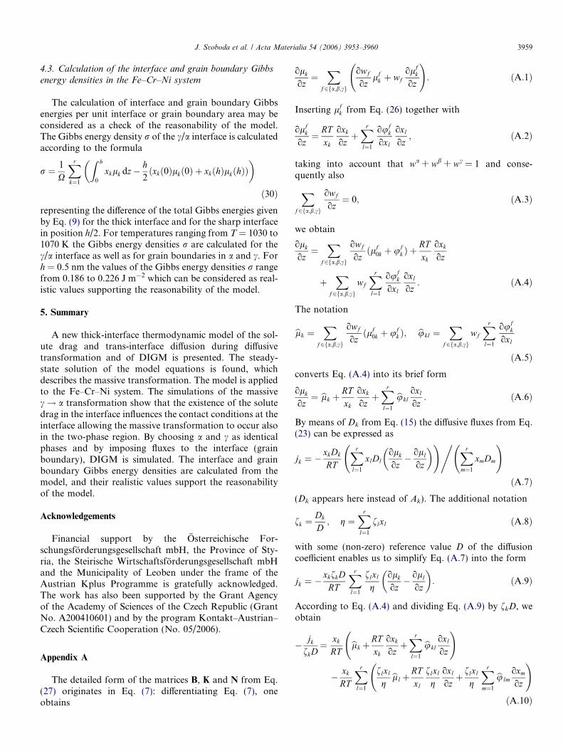
4.3. Calculation of the interface and grain boundary Gibbs

energy densities in the Fe–Cr–Ni system

The calculation of interface and grain boundary Gibbsenergies per unit interface or grain boundary area may beconsidered as a check of the reasonability of the model.The Gibbs energy density r of the c/a interface is calculatedaccording to the formula

r ¼ 1

X

Xr

k¼1

Z h

0

xklk dz� h2ðxkð0Þlkð0Þ þ xkðhÞlkðhÞÞ

� �ð30Þ

representing the difference of the total Gibbs energies givenby Eq. (9) for the thick interface and for the sharp interfacein position h/2. For temperatures ranging from T = 1030 to1070 K the Gibbs energy densities r are calculated for thec/a interface as well as for grain boundaries in a and c. Forh = 0.5 nm the values of the Gibbs energy densities r rangefrom 0.186 to 0.226 J m�2 which can be considered as real-istic values supporting the reasonability of the model.

5. Summary

A new thick-interface thermodynamic model of the sol-ute drag and trans-interface diffusion during diffusivetransformation and of DIGM is presented. The steady-state solution of the model equations is found, whichdescribes the massive transformation. The model is appliedto the Fe–Cr–Ni system. The simulations of the massivec! a transformation show that the existence of the solutedrag in the interface influences the contact conditions at theinterface allowing the massive transformation to occur alsoin the two-phase region. By choosing a and c as identicalphases and by imposing fluxes to the interface (grainboundary), DIGM is simulated. The interface and grainboundary Gibbs energy densities are calculated from themodel, and their realistic values support the reasonabilityof the model.

Acknowledgements

Financial support by the Osterreichische For-schungsforderungsgesellschaft mbH, the Province of Sty-ria, the Steirische Wirtschaftsforderungsgesellschaft mbHand the Municipality of Leoben under the frame of theAustrian Kplus Programme is gratefully acknowledged.The work has also been supported by the Grant Agencyof the Academy of Sciences of the Czech Republic (GrantNo. A200410601) and by the program Kontakt–Austrian–Czech Scientific Cooperation (No. 05/2006).

Appendix A

The detailed form of the matrices B, K and N from Eq.(27) originates in Eq. (7): differentiating Eq. (7), oneobtains

olk

oz¼

Xf2fa;b;cg

owf

ozlf

k þ wfolf

k

oz

!: ðA:1Þ

Inserting lfk from Eq. (26) together with

olfk

oz¼ RT

xk

oxk

ozþXr

l¼1

oufk

oxl

oxl

oz; ðA:2Þ

taking into account that wa + wb + wc = 1 and conse-quently alsoXf2fa;b;cg

owf

oz¼ 0; ðA:3Þ

we obtain

olk

oz¼

Xf2fa;b;cg

owf

ozðlf

0k þ ufk Þ þ

RTxk

oxk

oz

þX

f2fa;b;cgwf

Xr

l¼1

oufk

oxl

oxl

oz: ðA:4Þ

The notation

blk ¼X

f2fa;b;cg

owf

ozðlf

0k þ ufk Þ; bukl ¼

Xf2fa;b;cg

wf

Xr

l¼1

oufk

oxl

ðA:5Þconverts Eq. (A.4) into its brief form

olk

oz¼ blk þ

RTxk

oxk

ozþXr

l¼1

bukloxl

oz: ðA:6Þ

By means of Dk from Eq. (15) the diffusive fluxes from Eq.(23) can be expressed as

jk ¼ �xkDk

RT

Xr

l¼1

xlDlolk

oz� oll

oz

� � !, Xr

m¼1

xmDm

!ðA:7Þ

(Dk appears here instead of Ak). The additional notation

fk ¼Dk

D; g ¼

Xr

l¼1

flxl ðA:8Þ

with some (non-zero) reference value D of the diffusioncoefficient enables us to simplify Eq. (A.7) into the form

jk ¼ �xkfkD

RT

Xr

l¼1

flxl

golk

oz� oll

oz

� �: ðA:9Þ

According to Eq. (A.4) and dividing Eq. (A.9) by fkD, weobtain

� jk

fkD¼ xk

RTblk þ

RTxk

oxk

ozþXr

l¼1

bukloxl

oz

!

� xk

RT

Xr

l¼1

flxl

gbllþ

RTxl

flxl

goxl

ozþ flxl

g

Xr

m¼1

bulmoxm

oz

!ðA:10Þ

3960 J. Svoboda et al. / Acta Materialia 54 (2006) 3953–3960

and using the new notation

lk ¼ blk �Xr

l¼1

flxl

gbll; ukl ¼ bukl �

Xr

m¼1

fmxm

gbuml ðA:11Þ

finally

� jk

fkD¼ oxk

oz� xkfl

goxl

ozþ xklk

RTþ xk

Xr

l¼1

ukl

RToxl

oz: ðA:12Þ

From Eq. (25) it is known

jk

fkDþ v

fkDXðxk � x1k Þ ¼ 0; ðA:13Þ

this together with Eq. (A.12) yields

oxk

ozþ xk

Xr

l¼1

� fl

gþ ukl

RT

� �oxl

ozþ lk

RTþ v

fkDX

� �xk ¼

vfkDX

x1k :

ðA:14Þ

Clearly x1 + . . . + xr = 1, thus

oxr

oz¼ � ox1

oz� . . .� oxr�1

ozðA:15Þ

and also

g ¼Xr�1

l¼1

flxl þ fr 1�Xr�1

l¼1

xl

!¼ fr þ

Xr�1

l¼1

ðfl � frÞxl:

ðA:16Þ

Consequently the contribution of the summation with theindex r in Eq. (A.9) can be eliminated with the result

oxk

ozþ xk

Xr�1

l¼1

� fl

gþ ukl

RT

� �oxl

oz� xk

Xr�1

l¼1

� fr

gþ ukr

RT

� �oxl

oz

þ lk

RTþ v

fkDX

� �xk ¼

vfkDX

x1k ðA:17Þ

for k 2 {1, . . . , r � 1}; this can be rewritten as

oxk

ozþ xk

Xr�1

l¼1

Bkloxl

ozþ ðKk þ vN kÞxk ¼ vN kx1k ðA:18Þ

where

Bkl ¼xkðfr � flÞ

gþ ukl � ukr

RT; Kkk ¼

lk

RT; Nkk ¼

1

fkDX

ðA:19Þ

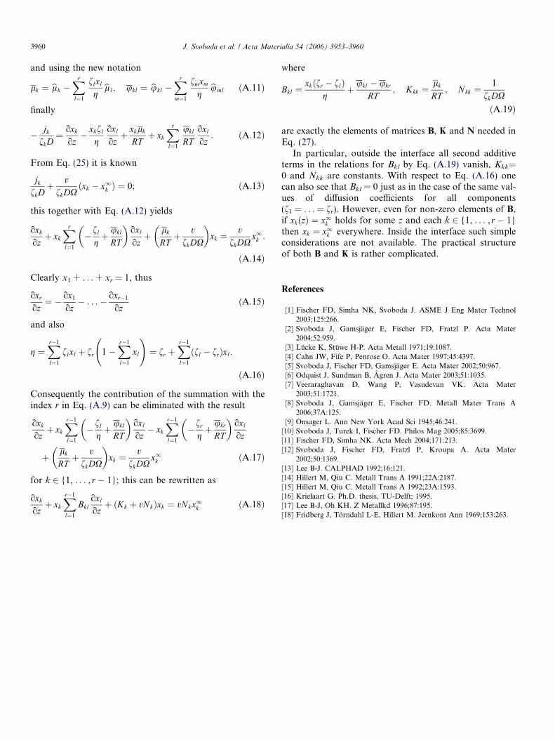
are exactly the elements of matrices B, K and N needed inEq. (27).

In particular, outside the interface all second additiveterms in the relations for Bkl by Eq. (A.19) vanish, Kkk=0 and Nkk are constants. With respect to Eq. (A.16) onecan also see that Bkl = 0 just as in the case of the same val-ues of diffusion coefficients for all components(f1 = . . . = fr). However, even for non-zero elements of B,if xkðzÞ ¼ x1k holds for some z and each k 2 {1, . . . , r � 1}then xk ¼ x1k everywhere. Inside the interface such simpleconsiderations are not available. The practical structureof both B and K is rather complicated.

References

[1] Fischer FD, Simha NK, Svoboda J. ASME J Eng Mater Technol2003;125:266.

[2] Svoboda J, Gamsjager E, Fischer FD, Fratzl P. Acta Mater2004;52:959.

[3] Lucke K, Stuwe H-P. Acta Metall 1971;19:1087.[4] Cahn JW, Fife P, Penrose O. Acta Mater 1997;45:4397.[5] Svoboda J, Fischer FD, Gamsjager E. Acta Mater 2002;50:967.[6] Odquist J, Sundman B, Agren J. Acta Mater 2003;51:1035.[7] Veeraraghavan D, Wang P, Vasudevan VK. Acta Mater

2003;51:1721.[8] Svoboda J, Gamsjager E, Fischer FD. Metall Mater Trans A

2006;37A:125.[9] Onsager L. Ann New York Acad Sci 1945;46:241.

[10] Svoboda J, Turek I, Fischer FD. Philos Mag 2005;85:3699.[11] Fischer FD, Simha NK. Acta Mech 2004;171:213.[12] Svoboda J, Fischer FD, Fratzl P, Kroupa A. Acta Mater

2002;50:1369.[13] Lee B-J. CALPHAD 1992;16:121.[14] Hillert M, Qiu C. Metall Trans A 1991;22A:2187.[15] Hillert M, Qiu C. Metall Trans A 1992;23A:1593.[16] Krielaart G. Ph.D. thesis, TU-Delft; 1995.[17] Lee B-J, Oh KH. Z Metallkd 1996;87:195.[18] Fridberg J, Torndahl L-E, Hillert M. Jernkont Ann 1969;153:263.