A THEORY OF ORDINARY P-ADIC CURVES

A Theory of Ordinary p-adic Curves

By

Shinichi MOCHIZUKI*

Table of Contents

Table of Contents

Introduction

§0. Statement of Main Results

§1. Review of the Complex TheoryBeltrami DifferentialsThe Beltrami EquationThe Series Expansion of a Quasiconformal FunctionUniformization of Hyperbolic Riemann SurfacesUniformization of Moduli Stacks of Hyperbolic Riemann SurfacesQuasidisks and the Bers EmbeddingThe Infinitesimal Form of the Modular UniformizationsCoordinates of DegenerationThe Parabolic CaseReal Curves

§2. Translation into the p-adic CaseGunning’s Theory of Indigenous BundlesThe Canonical Coordinates Associated to a Kahler MetricThe Weil-Petersson Metric from the Point of View of Indigenous BundlesThe Philosophy of Kahler Metrics as Frobenius LiftingsThe DictionaryLoose Ends

Received September 8, 1995. Revised October 2, 1996.

1991 Mathematics Subject Classification: 14H10, 14F30

* Research Institute for Mathematical Sciences, Kyoto University, Kyoto 606, Japan

1

Chapter I: Crystalline Projective Structures

§0. Introduction

§1. Schwarz StructuresNotation and Basic DefinitionsFirst Properties of Schwarz StructuresCrystalline Schwarz Structures and MonodromyCorrespondence with P1-bundlesSchwarz Structures and Square DifferentialsNormalized P1-bundles with ConnectionThe Schwarzian Derivative

§2. Indigenous BundlesBasic Definitions and ExamplesFirst PropertiesExistence and de Rham CohomologyIndigenous Bundles of Restrictable Type

§3. The Obstruction to Global IntrinsicityIntroduction of Cohomology ClassesComputation of the Second Chern ClassThe Case of Dimension One

Appendix: Relation to the Complex Analytic Case

Chapter II: Indigenous Bundles in Characteristic p

§0. Introduction

§1. FL-BundlesDeformations and FL-BundlesThe p-Curvature of an FL-Bundle

§2. The Verschiebung on Indigenous BundlesThe Definition of The VerschiebungThe p-Curvature of an Admissible Indigenous BundleThe Infinitesimal VerschiebungDifferential Criterion for Admissibility

2

§3. Hyperbolically Ordinary CurvesBasic DefinitionsThe Totally Degenerate CaseThe Case of Elliptic Curves: The Parabolic PictureThe Case of Elliptic Curves: The Hyperbolic PictureThe Generic Uniformization Number

Chapter III: Canonical Modular Frobenius Liftings

§0. Introduction

§1. Generalities on Ordinary Frobenius LiftingsBasic DefinitionsThe Uniformizing Galois RepresentationThe Canonical p-divisible GroupLogarithms of PeriodsCompatibility of DifferentialsCanonical Liftings of Points in Characteristic pCanonical Multiplicative ParametersCanonical Affine CoordinatesThe Relationship Between Affine and Multiplicative Parameters

§2. Construction of the Canonical Frobenius LiftingModular Frobenius LiftingsIndigenous Sections of DFrobenius Invariant Indigenous Bundles

§3. Applications of the Canonical Frobenius LiftingsCanonical Liftings of Curves over Witt VectorsCanonical Affine Coordinates on Mg,r

Topological Markings and Uniformization by Quadratic DifferentialsCanonical Multiplicative ParametersThe Case of Elliptic Curves

Chapter IV: Canonical Curves

§0. Introduction

3

§1. The Canonical Galois RepresentationConstruction and Global PropertiesThe Horizontal Section over the Ordinary LocusThe Canonical Frobenius Lifting over the Ordinary Locus

§2. The Canonical Log p-divisible GroupLog p-divisible Groups at InfinityConstruction of the Canonical Log p-divisible GroupReview of the Theory of [Katz-Mazur]

§3. The Compactified Canonical Frobenius LiftingThe Canonical Frobenius Lifting and the Canonical Log p-divisible GroupLocal Analysis at Supersingular PointsGlobal Hecke Correspondences

§4. p-adic Green’s FunctionsCompactified Frobenius LiftingsThe Height of a Frobenius LiftingAdmissible Frobenius LiftingsGeometric Criterion for Canonicality

Chapter V: Uniformizations of Ordinary Curves

§0. Introduction

§1. Crystalline InductionThe Crystalline-Induced MF∇-objectThe Ring of Additive PeriodsThe Crystalline-Induced Galois RepresentationRelation to the Canonical Affine CoordinatesThe Parabolic Case

§2. Canonical Objects over the Stack of Multiplicative PeriodsThe Stack of Multiplicative PeriodsThe Canonical Log p-divisible GroupThe Canonical Frobenius Lifting

BibliographyIndex

4

Introduction

§0. Statement of Main Results

The goal of this paper is to present a theory of r-pointed stable curves of genus g overp-adic schemes (for p odd), which, on the one hand, generalizes the Serre-Tate theory ofordinary elliptic curves to the hyperbolic case (i.e., 2g−2+r ≥ 1), and, on the other hand,generalizes the complex uniformization theory of hyperbolic Riemann surfaces (reviewed in§1 of this introductory Chapter) due to Ahlfors, Bers, et al. to the p-adic case. We begin bysetting up the necessary algebraic machinery: that is, the language of indigenous bundles(due to Gunning, although we rephrase Gunning’s results in a more algebraic form). Anindigenous bundle is a P1-bundle over a curve, together with a connection, that satisfycertain properties. One may think of an indigenous bundle as an algebraic way of encodinguniformization data for a curve. We then study the p-curvature of indigenous bundles incharacteristic p, and show that a generic r-pointed stable curve of genus g has a finite,nonzero number of distinguished indigenous bundles (P,∇P ), which are characterized bythe following two properties:

(1) the p-curvature of (P,∇P ) is nilpotent;

(2) the space of indigenous bundles with nilpotent p-curvature is etale overthe moduli stack of curves at (P,∇P ).

We call such (P,∇P ) nilpotent and ordinary, and we call curves ordinary if they admit atleast one such nilpotent, ordinary indigenous bundle. If a curve is ordinary, then choos-ing any one of the finite number of nilpotent, ordinary indigenous bundles on the curvecompletely determines the “uniformization theory of the curve” – to be described in thefollowing paragraphs. Because of this, we refer to this choice as the choice of a p-adicquasiconformal equivalence class to which the curve belongs.

After studying various basic properties of ordinary curves and ordinary indigenousbundles in characteristic p, we then consider the p-adic theory. Let Mg,r be the modulistack of r-pointed stable curves of genus g over Zp. Then we show that there exists acanonical p-adic (nonempty) formal stack N ord

g,r together with an etale morphism

N ord

g,r → Mg,r

such that modulo p, N ord

g,r is the moduli stack of ordinary r-pointed curves of genus g,together with a choice of p-adic quasiconformal equivalence class. Moreover, the genericdegree of N ord

g,r over Mg,r is > 1 (as long as 2g− 2 + r ≥ 1 and p is sufficiently large). It is

over N ord

g,r that most of our theory will take place. Our first main result is the following:

5

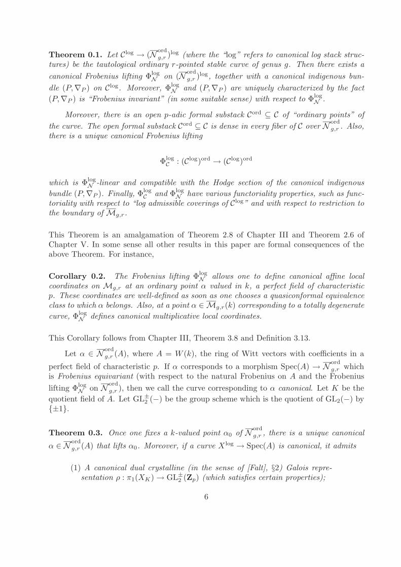
Theorem 0.1. Let Clog → (N ord

g,r )log (where the “log” refers to canonical log stack struc-tures) be the tautological ordinary r-pointed stable curve of genus g. Then there exists acanonical Frobenius lifting Φlog

N on (N ord

g,r )log, together with a canonical indigenous bun-dle (P,∇P ) on Clog. Moreover, Φlog

N and (P,∇P ) are uniquely characterized by the fact(P,∇P ) is “Frobenius invariant” (in some suitable sense) with respect to Φlog

N .

Moreover, there is an open p-adic formal substack Cord ⊆ C of “ordinary points” ofthe curve. The open formal substack Cord ⊆ C is dense in every fiber of C over N ord

g,r . Also,there is a unique canonical Frobenius lifting

ΦlogC : (Clog)ord → (Clog)ord

which is ΦlogN -linear and compatible with the Hodge section of the canonical indigenous

bundle (P,∇P ). Finally, ΦlogC and Φlog

N have various functoriality properties, such as func-toriality with respect to “log admissible coverings of Clog” and with respect to restriction tothe boundary of Mg,r.

This Theorem is an amalgamation of Theorem 2.8 of Chapter III and Theorem 2.6 ofChapter V. In some sense all other results in this paper are formal consequences of theabove Theorem. For instance,

Corollary 0.2. The Frobenius lifting ΦlogN allows one to define canonical affine local

coordinates on Mg,r at an ordinary point α valued in k, a perfect field of characteristicp. These coordinates are well-defined as soon as one chooses a quasiconformal equivalenceclass to which α belongs. Also, at a point α ∈ Mg,r(k) corresponding to a totally degeneratecurve, Φlog

N defines canonical multiplicative local coordinates.

This Corollary follows from Chapter III, Theorem 3.8 and Definition 3.13.

Let α ∈ N ord

g,r (A), where A = W (k), the ring of Witt vectors with coefficients in a

perfect field of characteristic p. If α corresponds to a morphism Spec(A) → N ord

g,r whichis Frobenius equivariant (with respect to the natural Frobenius on A and the Frobeniuslifting Φlog

N on N ord

g,r ), then we call the curve corresponding to α canonical. Let K be thequotient field of A. Let GL±

2 (−) be the group scheme which is the quotient of GL2(−) by{±1}.

Theorem 0.3. Once one fixes a k-valued point α0 of N ord

g,r , there is a unique canonical

α ∈ N ord

g,r (A) that lifts α0. Moreover, if a curve X log → Spec(A) is canonical, it admits

(1) A canonical dual crystalline (in the sense of [Falt], §2) Galois repre-sentation ρ : π1(XK) → GL±

2 (Zp) (which satisfies certain properties);

6

(2) A canonical log p-divisible group Glog (up to {±1}) on X log whose Tatemodule defines the representation ρ;

(3) A canonical Frobenius lifting ΦlogX : (X log)ord → (X log)ord over the

ordinary locus (which satisfies certain properties).

Moreover, if a lifting X log → Spec(A) of α0 has any one of these objects (1) through (3)(satisfying various properties), then it is canonical.

This Theorem results from Chapter III, Theorem 3.2, Corollary 3.4; Chapter IV, Theorem1.1, Theorem 1.6, Definition 2.2, Proposition 2.3, Theorem 4.17.

The case of curves with ordinary reduction modulo p which are not canonical is morecomplicated. Let us consider the universal case. Thus, let Slog = (N ord

g,r )log; let f log :X log → Slog be the universal r-pointed stable curve of genus g. Let T log → Slog bethe finite covering (log etale in characteristic zero) which is the Frobenius lifting Φlog

N ofTheorem 0.1. Let P log → Slog be the inverse limit of the coverings of Slog which areiterates of the Frobenius lifting Φlog

N . Let X logT = X log ×Slog T log; X log

P = X log ×Slog P log.We would like to consider the arithmetic fundamental groups

Π1def= π1((X

logT )Qp

); Π∞def= π1((X

logP )Qp

)

Unlike the case of canonical curves, we do not get a canonical Galois representation of Π1

into GL±2 (Zp). Instead, we have the following

Theorem 0.4. There is a canonical Galois representation

ρ∞ : Π∞ → GL±2 (Zp)

Moreover, the obstruction to extending ρ∞ to Π1 is nontrivial and is measured precisely bythe extent to which the canonical affine coordinates (of Corollary 0.2) are nonzero. Also,there is a ring DGal

S with a continuous action of π1(TlogQp

) such that we have a canonicaldual crystalline representation

ρ1 : Π1 → GL±2 (DGal

S )

(i.e., this is a twisted homomorphism, with respect to the action of Π1 (acting throughπ1(T

logQp

)) on DGalS ). Finally, the ring DGal

S has an augmentation DGalS → Zp which is

Π∞-equivariant (for the trivial action on Zp) and which is such that after restricting toΠ∞, and base changing by means of this augmentation, ρ1 reduces to ρ∞.

7

This follows from Chapter V, Theorems 1.4 and 1.7.

All along, we note that when one specializes the theory to the case of elliptic curves,one recovers the familiar classical theory of Serre-Tate. For instance, the definitions of“ordinary curves” and “canonical liftings” specialize to the objects with the same namesin Serre-Tate theory. The p-adic canonical coordinates on the moduli stack Mg,r (Corollary0.2) specialize to the Serre-Tate parameter. The Galois obstruction to extending ρ∞ toa representation of Π1 specializes to the obstruction to splitting the well-known exactsequence of Galois modules that the p-adic Tate module of an ordinary elliptic curve fitsinto.

For more detailed accounts of the results in each Chapter, we refer to the introductorysections at the beginnings of each of the Chapters. In the rest of this introductory Chapter,we explain the relationship between the p-adic case and the classically known complex case.

Acknowledgements: I would like to thank Prof. Barry Mazur of Harvard University forproviding the stimulating environment (during the Spring of 1994) in which this paperwas written. Also, I would like to thank both Prof. Mazur and Prof. Yasutaka Ihara(of RIMS, Kyoto University) for their efforts in assisting me to publish this paper, andfor permitting me to hold lecture series at Harvard (Spring of 1994) and RIMS (Fall of1994), respectively, during which I discussed the contents of this paper. Finally, I wouldlike to thank Prof. Ihara for informing me of the theory of [Ih], [Ih2], [Ih3], and [Ih4].This theory anticipates many aspects of the theory of the present paper (especially, thediscussion of Frobenius liftings and pseudo-correspondences in Chapters III and IV). Onthe other hand, the techniques and point of view of Prof. Ihara’s theory differ substantiallyfrom those of the present paper. Moreover, from a rigorous, mathematical point of view,the main results of Prof. Ihara’s theory neither imply nor are implied by the main resultsof the present paper. However, it is the author’s subjective opinion that philosophically,the motivation behind Prof. Ihara’s theory was much the same as that of the author’s.

§1. Review of the Complex Theory

In order to explain the meaning of the main results of this paper, it is first necessaryto review the complex theory of uniformization in a fashion that makes the generalizationto finite primes more natural. This is the goal of the present Section. Since all of thematerial is “standard” and “well-known,” we shall, of course, omit proofs, instead citingreferences for major results. We shall say that a Riemann surface X is of finite typeif it can be obtained by removing a finite number of points p1, . . . , pr from a compactRiemann surface Y of genus g. Note that in this case, Y and {p1, . . . , pr} are uniquelydetermined up to isomorphism. We shall say that the Riemann surface of finite type X ishyperbolic (respectively, parabolic; elliptic) if 2g − 2 + r ≥ 1 (respectively, 2g − 2 + r = 0;2g − 2 + r < 0). In this paper, we shall be concerned exclusively with Riemann surfacesof finite type (and their uniformizations). This is because it is precisely these Riemannsurfaces which correspond to algebraic objects. Also, we shall mainly be concerned with

8

the hyperbolic case, since this is the most difficult. Indeed, from the point of view ofthe theory of uniformization and moduli, the elliptic case is completely trivial, and theparabolic case (although nontrivial) is relatively easy and explicit.

In some sense, the theme of our review of the classical complex theory is that in mostcases, there are two ways to approach results: the “classical” and the “quasiconformal.”Typically, the classical approach was known earlier, and is more geometric and intuitive.On the other hand, the classical approach has the drawback of producing theories andresults that are only real analytic, rather than holomorphic in nature. By contrast thequasiconformal approach, which was pioneered by Ahlfors and Bers, tends to give rise toholomorphic structures and results naturally. It is thus natural that the connection betweenthe “quasiconformal approach” and the p-adic theory should be much more natural andtransparent.

Beltrami Differentials

Let X be a Riemann surface (not necessarily of finite type). Let us consider thecomplex line bundle τX ⊗ ωX on X, where ωX is the complex conjugate bundle to thecanonical bundle ωX , and τX is the tangent bundle. Note that if s is a section of τX ⊗ωX

over X, then we can consider its L∞-norm ‖s‖∞, since the transition functions of τX ⊗ωX

have complex absolute value 1. A Beltrami differential μ on X is a measurable section ofthe line bundle

τX ⊗ ωX

such that ‖μ‖∞ < 1.

Why the bundle τX ⊗ ωX? The reason is that this bundle is closely connected withthe moduli of the Riemann surface X. Indeed, Let us consider an arbitrary C∞ section μof τX ⊗ ωX . Now since τX has the structure of a holomorphic line bundle, we have a ∂operator on τX . If we look at global C∞ sections, this gives us a complex

C∞(X, τX) ∂−→ C∞(X, τX ⊗ ωX)

which computes the analytic cohomology of τX . If X is, for instance, compact, then thisanalytic cohomology coincides with the cohomology in the Zariski topology of the algebraictangent bundle. Thus, for X compact and hyperbolic, the above complex has cohomologygroups H0 = 0, and H1 = H1(X, τX), which is well-known to be the space of infinitesimaldeformations of X. Moreover, if X is compact of genus g ≥ 2, and Mg is the moduli stackof curves of genus g, then H1(X, τX) is precisely the tangent space to Mg at the pointdefined by X.

At any rate, (for X arbitrary) we have a natural surjection

9

C∞(X, τX ⊗ ωX) → H1(X, τX)

Thus, the image of μ under this surjection defines an infinitesimal deformation of thecomplex structure of X. This establishes the relationship between sections of

τX ⊗ ωX

and the moduli of X. The reason for considering measurable, rather than just C∞, sec-tions is that it is easier to obtain solutions to a certain differential equation, the Beltramiequation, when one works in this greater generality.

The Beltrami Equation

Having established the relationship between sections of τX ⊗ ωX and infinitesimaldeformations, we now would like to integrate – i.e., to “give a reciprocity law” – thatassigns to a section μ of τX ⊗ωX not just an infinitesimal deformation of X, but an actualnew Riemann surface, i.e., a new complex structure on the topological manifold underlyingX. To do this, we consider the Beltrami equation

∂f = μ · ∂f

which we regard as a differential equation in the unknown function f . It is a nontrivialresult (proven, for instance, in [Lehto2]) that when μ is a Beltrami differential, thereexist local L2 solutions f to the Beltrami equation that are homeomorphisms (where theyare defined). Such functions f are called quasiconformal (with dilatation μ). If f andg (defined on some open set U ⊆ X) are both quasiconformal with the same dilatationμ, then it is easy to see that ∂ applied to f ◦ g−1 (in the distributional sense) is zero.That is, f = h ◦ g for some biholomorphic function h. Thus, up to composition with abiholomorphic function, quasiconformal solutions to the Beltrami equation are unique.

With these observations, we can define a new complex structure on X associated toa Beltrami differential μ as follows. Let us call the resulting Riemann surface Xμ. Thus,the underlying topological manifold of Xμ is the same as that of X. On an open setU ⊆ X, we take a local quasiconformal function f of dilatation μ, and define it to bea holomorphic function on Xμ. By the essential uniqueness of solutions to the Beltramiequation, everything is well-defined, and so we obtain a new global Riemann surface Xμ.Thus, the assignment

μ → Xμ

is the fundamental “reciprocity law” that we are looking for.

10

The Series Expansion of a Quasiconformal Function

In order to really understand the Beltrami equation, it is useful to look at the explicitrepresentation of its solutions as series “in μ” (as in [Lehto], pp. 25-27). We begin byconsidering Cauchy’s integral formula:

f(z) =1

2πi

∫∂D

f(ζ) dζ

ζ − z− 1

π

∫ ∫D

∂f(ζ) dξdη

ζ − z

for a function f with L1 derivatives on an open disk D in the complex plane. Thus, if f(and its L1 derivatives) are defined on all of C, and f(z) → 0 as z → ∞, then we obtain

f(z) = T ∂f

where T is the operator on C∞ functions ω with compact support given by

(T ω)(z) = − 1π

∫ ∫C

ω(ζ) dξdη

ζ − z

Put another way, (from the point of view of the theory of pseudodifferential operators) Tis the parametrix for the elliptic differential operator ∂. If we define the Hilbert transfor-mation H by

(H ω)(z) = − 1π

∫ ∫C

ω(ζ) dξdη

(ζ − z)2

then we obtain that ∂T = H. Also, it can be shown that ∂ and ∂ commute with both Tand H.

Now let us suppose that μ is a Beltrami differential on C (say, with compact support),and that f is quasiconformal on C with dilatation μ. Then f is holomorphic at infinity,and so, after normalization, in a neighborhood of infinity, it looks like

f(z) = z +∑n≥1

bnz−n

for some bn ∈ C. Thus, f(z) − z goes to 0 as z → ∞, so we obtain that

∂f(z) = 1 + ∂{f(z) − z}= 1 + ∂T∂{f(z) − z}= 1 + H∂f(z)

11

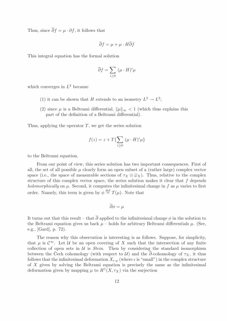
Thus, since ∂f = μ · ∂f , it follows that

∂f = μ + μ · H∂f

This integral equation has the formal solution

∂f =∑i≥0

(μ · H)iμ

which converges in L2 because

(1) it can be shown that H extends to an isometry L2 → L2;

(2) since μ is a Beltrami differential, ‖μ‖∞ < 1 (which thus explains thispart of the definition of a Beltrami differential).

Thus, applying the operator T , we get the series solution

f(z) = z + T{∑i≥0

(μ · H)iμ}

to the Beltrami equation.

From our point of view, this series solution has two important consequences. First ofall, the set of all possible μ clearly form an open subset of a (rather large) complex vectorspace (i.e., the space of measurable sections of τX ⊗ ωX). Thus, relative to the complexstructure of this complex vector space, the series solution makes it clear that f dependsholomorphically on μ. Second, it computes the infinitesimal change in f as μ varies to firstorder. Namely, this term is given by φ

def= T (μ). Note that

∂φ = μ

It turns out that this result – that ∂ applied to the infinitesimal change φ in the solution tothe Beltrami equation gives us back μ – holds for arbitrary Beltrami differentials μ. (See,e.g., [Gard], p. 72).

The reason why this observation is interesting is as follows. Suppose, for simplicity,that μ is C∞. Let U be an open covering of X such that the intersection of any finitecollection of open sets in U is Stein. Then by considering the standard isomorphismbetween the Cech cohomology (with respect to U) and the ∂-cohomology of τX , it thusfollows that the infinitesimal deformation Xε·μ (where ε is “small”) in the complex structureof X given by solving the Beltrami equation is precisely the same as the infinitesimaldeformation given by mapping μ to H1(X, τX) via the surjection

12

C∞(X, τX ⊗ ωX) → H1(X, τX)

considered previously. This completes the justification of the claim that the assignmentμ → Xμ is an “integrated version” of the “infinitesimal reciprocity law”

C∞(X, τX ⊗ ωX) → H1(X, τX)

that follows just from the definition of the ∂-cohomology of τX .

Uniformization of Hyperbolic Riemann Surfaces

Let X be a hyperbolic Riemann surface. Let X be its universal covering space. Thus,X inherits a natural complex structure from X. Then one of the most basic results in thefield is that we have an isomorphism of Riemann surfaces

X ∼= H

where H is the upper half plane. By considering the covering transformations of H → X,we get a homomorphism (well-defined up to conjugation)

ρ : π1(X) → Aut(H) ⊆ PSL2(R)

which we call the canonical representation of X.

There are (at least) two ways to prove this result. The first approach is the classicalapproach, and goes back to Koebe’s work in the early twentieth century. It involvesconsidering Green’s functions G(−,−) on X. There is an intrinsic, a priori definition ofGreen’s functions, which is not important for us here. A posteriori, that is, once one knowsthat X ∼= H, we can pull-back the hyperbolic metric

dx2 + dy2

y2

on H to X, so that we obtain a hyperbolic distance function on X. Then G(x, y) (forx, y ∈ X) is given by the logarithm of the hyperbolic distance between x and y. One canfind a detailed exposition of this approach in [FK].

The second approach (which is more relevant to the p-adic case) is the approach ofBers ([Bers]). Suppose that X is obtained by removing r points from a compact Riemannsurface Y of genus g. Then one first observes that there exists a Riemann surface X ′

which is obtained by removing r points from a compact Riemann surface of genus g andwhose universal covering space X ′ is isomorphic to H. Then one constructs (from purely

13

elementary considerations) a quasiconformal homeomorphism X ′ ∼= X. This quasiconfor-mal homeomorphism defines a Beltrami differential μ on X ′, which we can pull back toX ′ ∼= H to obtain a Beltrami differential μH on H. By reflection, one extends μH to aBeltrami differential μ on C. Then we solve the Beltrami equation for μ on C so that weobtain a quasiconformal homeomorphism

fμ

: C → C

which goes to infinity at infinity. Let Γ′ be the group of Mobius transformation of Hdefined by the covering transformations of X ′ over X ′. Thus, H/Γ′ ∼= X ′. Then it followsfrom the uniqueness of solutions to the Beltrami equation that

Γ def= fμ◦ Γ′ ◦ f−1

μ

forms a group of Mobius transformations on C. Moreover, from the reflection symmetryof μ, it follows that f

μpreserves the real axis, and hence so does Γ. It thus follows that

H/Γ is a Riemann surface of finite type, and, by the definition of μ, that H/Γ ∼= X. Thiscompletes the proof.

It turns out that it is this approach of uniformizing a single Riemann surface (for eachg, r) and then “parallel transporting” the result over the rest of the moduli space that willcarry over to the p-adic case.

Uniformization of Moduli Stacks of Hyperbolic Riemann Surfaces

Let Mg,r be the moduli stack of r-pointed smooth algebraic curves of genus g over C.Let Mg,r be its universal covering space. Then the problem of uniformization of moduli isto give an explicit representation of Mg,r. From the point of view of the Beltrami equation,this amounts to finding a small, finite-dimensional subspace T of the space of Beltramidifferentials μ such that the assignment μ → Xμ defines a covering space map T → Mg,r.

We begin by fixing a “base point” of Mg,r, which corresponds to a hyperbolic Riemannsurface X. Let M(X) be the space of Beltrami differentials on X. Let Q be the spaceof holomorphic quadratic differentials on X with at most simple poles at the puncturedpoints. Then there are two approaches to defining morphisms from open subsets of Qinto spaces of Beltrami differentials. The first approach is that of Teichmuller. In thisapproach, if φ ∈ Q, we define a norm

‖φ‖ def=∫

X

|φ|

Let V ⊆ Q be the set of φ with ‖φ‖ ≤ 1. Then Teichmuller’s uniformization map, for(nonzero) φ ∈ V , is given by

14

φ → μφdef= (‖φ‖) φ

|φ|

where φ ∈ Γ(X,ω⊗2X ) is the complex conjugate of φ. It is easy to see that μφ defines a

Beltrami differential on X. Thus, we get a morphism V → M(X). If we compose φ → μφ

with μ → Xμ, we get a morphism

V → Mg,r

The main result of Teichmuller theory (see, e.g., [Gard], Chapter 6) is that this morphisminduces an isomorphism of V onto Mg,r. One advantage of this approach is that it admitsa very satisfying geometric interpretation in terms of a foliation on X induced by φ anddeforming X into Xμφ

by deforming a canonical coordinate arising from the foliation. Themain disadvantage of this approach from our point of view, however, is that the morphismφ → μφ is neither holomorphic nor anti-holomorphic. Thus, it seems hopeless to try tofind an algebraic version of Teichmuller’s map.

On the other hand, Bers’ approach is as follows. Since we now know that X canbe uniformized by the upper half plane, let vX be the hyperbolic volume element on Xinduced by the hyperbolic volume element

vH =dx ∧ dy

y2

on the upper half plane. Let Xc be the conjugate Riemann surface to X. That is, theunderlying topological manifold of Xc is the same as that of X, but the holomorphicfunctions on Xc are exactly the anti-holomorphic functions on X. Suppose that φ ∈ Q.Then by conjugating the “input variable,” we obtain that φ defines a section φc of ω⊗2

Xc .Now define

μφdef=

−2φc

vXc

Then for some appropriate (see [Gard], pp. 100-104) open set V ⊆ Q, this μφ definesa Beltrami differential on Xc. Integrating, we get a Riemann surface Xc

μ. Then theassignment φ → Xc

μ defines a morphism

V → Mcg,r

where the superscript “c” denotes the conjugate complex manifold. This morphism inducesan isomorphism of V onto Mc

g,r ([Gard], p. 101). The important thing here is that thecorrespondence φ → μφ is holomorphic. Since μ → Xc

μ is always holomorphic, it thus

15

follows that the isomorphism V ∼= Mcg,r is biholomorphic. Put another way, we have a

holomorphic embedding

B : Mg,r ↪→ Qc

which is called the Bers embedding. This embedding will be central to our entire treatmentof the complex theory, and its p-adic analogue will be central to our treatment of the p-adictheory.

Quasidisks and the Bers Embedding

One can also define the Bers embedding in terms of Bers’ simultaneous uniformizationand Schwarzian derivatives. For details, see [Gard], pp. 100-101. To do this, we fix anisomorphism of X with H. Let Hc be the lower half plane. Thus, if H uniformizes X,then Hc naturally uniformizes Xc. Let Γ be the group of Mobius transformiations of Cwhich are the covering transformations for H = X → X. Then we may think of the spaceM(Xc) of Beltrami differentials on Xc as the space of Beltrami differentials on Hc whichare invariant under Γ. Let μ ∈ M(Xc). Let fμ : C → C be the unique quasiconformalhomeomorphism which fixes 0 and 1, goes to infinity at infinity, has Beltrami coefficient μon Hc and is conformal on H. Let Γμ = fμ◦Γ◦(fμ)−1. Then it follows from the uniquenessof solutions to the Beltrami equation that Γμ forms a group of Mobius transformations ofC. Moreover, we have conformal isomorphisms

fμ(Hc)/Γμ ∼= Xcμ; fμ(H)/Γμ ∼= X

It follows that if we take the Schwarzian derivative of the conformal “quasidisk” embedding

fμ|H : H ↪→ C

we get a Γ-invariant quadratic differential on H, hence a quadratic differential φ (with atmost simple poles at the punctures) on X. The content of the Lemma of Ahlfors-Weill([Gard], p. 100) is that the assignment:

Xcμ → φ

is equal to Bc : Mcg,r ↪→ Q. On the one hand, this description of the Bers embedding is

geometrically more satisfying than the definition given in the previous subsection, but ithas the disadvantage that it obscures the relationship between the hyperbolic and paraboliccases. So far we have been mainly discussing the hyperbolic case, but we shall discuss theparabolic case later.

16

The Infinitesimal Form of the Modular Uniformizations

Often it is useful to express these modular uniformizations in their infinitesimal form,as metrics. On the one hand, the global uniformizations can always be essentially recoveredby integrating the metrics, and on the other hand, metrics, being local in nature, can oftenbe studied more easily.

In the Teichmuller case, if K is defined by

‖φ‖ =K − 1K + 1

then one obtains a distance function on Mg,r, given by

d(X,Xμφ) =

12log(K)

which turns out to be equal to the general hyperbolic distance introduced by Kobayashifor an arbitrary hyperbolic complex manifold (see [Gard], Chapter 7, for an exposition).The infinitesimal form of this distance is given by the norm ‖φ‖ =

∫X

|φ| on quadraticdifferentials (see [Royd]).

We shall be more interested in the case of the Bers embedding

B : Mg,r ↪→ Qc

By using the hyperbolic volume form vX on X, we obtain the Weil-Petersson inner product:

〈φ,ψ〉 def=∫

X

φ · ψvX

for φ, ψ ∈ Q. It is a result of Weil and Ahlfors that the resulting metric, called the Weil-Petersson metric on Mg,r, is Kahler. Moreover, if we differentiate B, we get, at X, a mapon tangent spaces

dB : Q∨ → Qc

whose inverse is exactly the morphism Qc → Q∨ defined by the Weil-Petersson inner prod-uct. Finally, the coordinates obtained from the Bers embedding are canonical coordinatesfor the Weil-Petersson metric ([Royd]). (We shall review the general theory of canonicalcoordinates associated to a real analytic Kahler metric in §2.)

It turns out that it is precisely the p-adic analogue of the Weil-Petersson metric thatwill play a central role in this paper.

17

Coordinates of Degeneration

While the Bers coordinates are useful for understanding what happens in the interiorof Mg,r, they are not so useful for understanding what happens as one goes out to theboundary, that is, as the Riemann surface degenerates to a Riemann surface with nodes.To study this sort of degeneration, one fixes a decomposition of the Riemann surface into“pants,” which are topologically equivalent to an open disk with two smaller disks in theinterior removed. For a detailed description of the theory of pants and the coordinates theydefine, we refer to [Abikoff], Chapter 2. In summary, what happens is the following. LetX be a hyperbolic Riemann surface (of genus g with r punctures), with a decompositioninto pants. We shall call the curves on X which occur in the boundary of the pantspartition curves. There are exactly 3g − 3 + r partition curves, α1, . . . , α3g−3+r. Weassume that this decomposition is “maximal” in the sense that each partition curve isa simple closed geodesic (in the hyperbolic metric on X). Then it turns out that theisomorphism class of X as a Riemann surface is completely determined by 3g − 3 + rcomplex numbers ζi = li eiθ (i = 1, . . . , 3g − 3 + r), one for each partition curve. Basicallyli describes the circumference of the partition curve αi, while θi describes the angle oftwisting involved in gluing together the boundary curves of two neighboring pants to formαi. These coordinates ζi are called the Fenchel-Nielsen coordinates of X. The degenerationcorresponding to pinching αi to a node is given by li → 0. This degeneration respects thehyperbolic metrics involved: that is, if a family of smooth Xt degenerates to a nodalRiemann surface Z, then the hyperbolic metrics on the Xt degenerate to the hyperbolicmetric on Z (given by taking the hyperbolic metric on the smooth subsurface of Z whichis the complement of the nodes). Thus, the Fenchel-Nielsen coordinates have the virtueof admitting a very satisfying differential-geometric description (as just summarized), butthe disadvantage of not being holomorphic.

On the other hand, one can define holomorphic coordinates (as in [Wolp]), as follows.Recall the quasidisk description of the Bers embedding. Thus, we had a μ ∈ M(Xc),and a quasiconformal homeomorphism fμ : C → C, together with a new group of Mobiustransformations Γμ. Then each αi defines (by integration) an element Ai ∈ Γμ. Up toconjugation, Ai is of the form z → mi · z for some mi ∈ C with |mi| > 1. This complexnumber mi is uniquely defined. Then the coordinates

Xcμ → (m1, . . . ,m3g−3+r)

are holomorphic in μ. In [Wolp], the relationship between these coordinates and the Berscoordinates is studied. In these coordinates, the degeneration of Xc

μ corresponding to thecase where the partition curve αi is pinched to a node is given by mi → 1. It turnsout that these coordinates are probably the best complex analogue to the “multiplicativeparameters at infinity” that we construct in the p-adic case.

18

The Parabolic Case

So far we have mainly been discussing the case of hyperbolic Riemann surfaces, sincethis case is by far the most interesting. However, often it is very difficult to make explicitcomputations for hyperbolic Riemann surfaces. Thus, in order to get one’s bearings, itis sometimes useful to consider the analogous constructions in the parabolic case, whereexplicit computations are much easier to carry out. Let X be a parabolic Riemann surface.Then X is either compact of genus 1, or it is isomorphic to the projective line minus twopoints. We shall mainly be interested in the compact case, where there are nontrivialmoduli.

Thus, let X be compact of genus 1. Then one can carry out Teichmuller theory inthis case (as in [Lehto], Chapter V, §6). One can also define a parabolic analogue of theBers embedding, as follows. Namely, we simply copy the formula

μφdef=

−2φc

vXc

of the hyperbolic case, except that we take vXc to be the parabolic volume element (asopposed to the hyperbolic volume element) on Xc, with

∫Xc vXc = 1. Then one sees (as

in [Lehto], p. 220) that one obtains a holomorphic embedding

B1,0 : M1,0 ↪→ Qc

whose image is an open disk D ⊆ Qc of some radius. One can also define a Weil-Peterssonmetric on M1,0 by simply replacing the hyperbolic volume element used before by theparabolic volume element. A simple calculation then reveals that one obtains the standardhyperbolic metric on the open disk D. In particular, (just as in the hyperbolic case), thestandard coordinate on D is normal at 0 for the Weil-Petersson metric.

One thing that is interesting about this parabolic case is that even though the complexanalytic stacks M1,0 and M1,1 are isomorphic, the “Bers theory” differs substantially inthe two cases. For instance, the Bers embedding of M1,1 is far from being an open disk.In fact, (as the author was told by C. McMullen) the boundary of this hyperbolic Bersembedding has lots of cusps. A computer-generated illustration of this boundary appears in[McM]. Also, it is not difficult to show that the Weil-Petersson metrics are quite different.This contrasts considerably with the “Teichmuller theory” of M1,0 and M1,1: Indeed,since Teichmuller’s metric always coincides with Kobayashi’s intrinsic hyperbolic metric,it follows that the Teichmuller metrics of M1,0 and M1,1 coincide.

Real Curves

A Riemann surface X of finite type is called real if X ∼= Xc. In other words, this meansthat the C-valued point defined by X in the algebraic stack (Mg,r)R (over Spec(R)) is,

19

in fact, defined over R (up to perhaps reordering the marked points). Various interestingproperties of real Riemann surfaces (related to uniformization theory) are studied in [Falt2].Many of these properties are obtained by looking at various one-dimensional real analyticsubmanifolds of a real X.

From our point of view, however, the notable fact about real hyperbolic Riemannsurfaces X is the following. Let φ : X ∼= Xc be a holomorphic isomorphism. For simplicity,suppose that there exists a point x ∈ X such that φ(x) = xc, and that φc ◦ φ = idX . Fixan isomorphism X ∼= H. This induces an isomorphism Xc ∼= Hc. On the other hand, φinduces a holomorphic isomorphism φ : H → Hc. Let C : Hc → H be the conjugationmap. Let ψ = C ◦ φ. Thus, ψ is an anti-holomorphic automorphism of H. Now letΠC = π1(X,x). Since Xc has the same underlying topological space as X, we haveΠC = π1(Xc, xc). Thus, φ induces an automorphism φΠ of ΠC of degree 2. Let ΠR be theextension

1 → ΠC → ΠR → Gal(C/R) → 1

which is the crossed product of ΠC with Gal(C/R) given by letting the nontrivial elementof Gal(C/R) act on ΠC by means of φΠ. Now let us consider the Lie group

G(R) def= {M ∈ GL2(R)| det(M) = ±1}/{±1}

Thus, PSL2(R) ⊆ G(R) ⊆ GL±2 (R), so we can write

ρC : ΠC → GL±2 (R)

for the canonical representation of X (uniformized by the upper half plane H). Note that

the full group GL±2 (R) acts on the upper half plane as follows: if A =

(a b

c d

)∈ GL±

2 (R),

we let

A(z) =aw + b

cw + d

where w = z (respectively, w = z) if det(A) is positive (respectively, negative). Thus,the map defined by A is a holomorphic (respectively, anti-holomorphic) automorphismof H if det(A) is positive (respectively, negative). In particular, the anti-holomorphicautomorphism ψ : H → H defines an element (which by abuse of notation we call) ψ ∈G(R). Now note that if γ ∈ ΠC, then ψ · ρ(γ) · ψ−1 = ρ(φΠ(γ)). Thus, by mapping thenontrivial element of Gal(C/R) in the crossed product definition of ΠR to ψ, we see thatwe obtain a natural homomorphism

ρR : ΠR → GL±2 (R)

20

which extends ρC and is such that the composite with the determinant det : GL±2 (R) →

R× is trivial on ΠC and equal to the sign representation on Gal(C/R). It is this repre-sentation ρR that will be relevant to our discussion of the p-adic case.

§2. Translation into the p-adic Case

In this Section, we discuss the dictionary for translating the complex analytic theoryof §1 into the p-adic results discussed in §0. Undoubtedly, the most fundamental tool,which is, in fact, of an algebraic, not an arithmetic nature, is the systematic use of theindigenous bundles of [Gunning]. This enables one to get rid of the upper half plane, andthus to bring uniformization theory into a somewhat more algebraic setting. In any sortof nontrivial arithmetic theory of this nature, however, algebraic manipulations alone cannever be enough. Thus, the fundamental arithmetic observation is the following:

Kahler metrics in the complex case correspond to Frobenius actions inthe p-adic case.

Since one typically gets a natural Frobenius action for free modulo p, a Frobenius actiontypically means a canonical lifting of the natural Frobenius action modulo p. In fact,in some sense, if one sorts through the complex analytic theory reviewed §1, one canessentially distill everything down to two objects, both of which happen to be Kahlermetrics:

(1) the hyperbolic metric on a hyperbolic Riemann surface (which encodesthe upper half plane uniformization); and

(2) the Weil-Petersson metric on the moduli space (which encodes the Bersuniformization).

Moreover, these two metrics are related to each other in the sense that the latter is essen-tially the push-forward of the former. In a similar way, the p-adic theory revolves aroundtwo fundamental Frobenius liftings:

(1) the canonical Frobenius lifting on a canonical hyperbolic curve; and

(2) the canonical Frobenius lifting on a certain stack which is etale overthe moduli stack.

The goal of this Section is to explain this analogy in greater detail.

21

Gunning’s Theory of Indigenous Bundles

Let X be a compact hyperbolic Riemann surface. Let H → X be its uniformizationby the upper half plane. Then by considering the covering transformations of H → X, weget a homomorphism (unique up to conjugation)

ρ : π1(X) → Aut(H) ⊆ PSL2(R)

which we call the canonical representation of X. If we regard ρ as defining a morphisminto PSL2(C), then we obtain (in the usual fashion), a local system of P1-bundles on X,which thus gives us a holomorphic P1-bundle with connection (P,∇P ) on X. By Serre’sGAGA, (P,∇P ) is necessarily algebraic. It turns out that P is always isomorphic to acertain P1-bundle of jets (which is also entirely algebraic). Thus, the upper half planeuniformization may be thought of as just being a special choice of connection ∇P . A pair“like” (P,∇P ) (satisfying certain technical properties discussed in Chapter I, §2) is calledan indigenous bundle. By working with log structures, one can also define indigenousbundles in a natural way for smooth X with punctures, as well as for nodal X.

As emphasized earlier, the point of dealing with indigenous bundles is that they allowone to translate the upper half plane uniformization into the purely algebraic informationof a connection on P . Of course, how one chooses this particular special connection on Pis very nontrivial arithmetic issue. We shall call the pair (P,∇P ) consisting of P equippedwith this particular connection the canonical indigenous bundle on X. Universally, overthe moduli stack Mg,r (of stable r-pointed curves of genus g over C), the space of allindigenous bundles forms a holomorphic torsor

Sg,r → Mg,r

over the logarithmic cotangent bundle Ωlog

Mg,r/Cof Mg,r. In the holomorphic category,

we shall see (in Chapter I, §3) that this torsor is highly nontrivial. In the real analyticcategory, however, the canonical indigenous bundle determines a trivializing section

sH : Sg,r → Mg,r

of this torsor.

In fact, indigenous bundles also allow us to translate such differential-geometric in-formation as the hyperbolic geometry of X into algebraic terms. For instance, considerthe degeneration of Riemann surfaces from the point of view of hyperbolic geometry. Asreviewed in §1, this may be thought of in terms of certain geodesic partition curves whoselengths go to zero as a family of smooth Xt degenerates to a nodal Riemann surface Z.From the complex theory, we know that the hyperbolic metric on Xt degenerates to thehyperbolic metric on Z. Using indigenous bundles, we can translate this into a more al-gebraic statement as follows: We define the canonical indigenous bundle on Z to be the

22

indigenous bundle obtained by gluing together the canonical indigenous bundles of thepointed Riemann surfaces occurring in the normalization of Z. Then the statement is thatas Xt degenerates to Z, the canonical indigenous bundle on Xt degenerates to the canon-ical indigenous bundle on Z. The statement that the lengths of the partition geodesicsgo to zero then takes the form that the monodromy of the limit indigenous bundle of thecanonical indigenous bundles of the Xt’s is nilpotent at the nodes.

The Canonical Coordinates Associated to a Kahler Metric

In this subsection we discuss how a Kahler metric on a complex manifold can be used todefine canonical affine, holomorphic coordinates on the manifold locally in a neighborhoodof a given point. We believe that what is discussed here is well-known, but our point ofview is somewhat different from that usually taken in the literature.

Let M be a smooth complex manifold of complex dimension m. The complex analyticstructure on M defines, in particular, a real analytic structure on M . Let μ be a realanalytic (1, 1)-form on M that defines a Kahler metric on M . In particular, μ is a closeddifferential form. Let M c be the conjugate complex manifold to M : that is to say, we takeM c to be that complex manifold which has the same underlying real analytic manifoldstructure as M , but whose holomorphic functions are the anti-holomorphic functions ofM . Let us fix a point e ∈ M . Let N be the germ of a complex manifold obtained bylocalizing the complex manifold M c × M at (e, e) ∈ M c × M (where this last expressionmakes sense since M c has the same underlying set as M). Let Ωhol (respectively, Ωant) bethe holomorphic vector bundle on N obtained by pulling back the bundle ΩM (respectively,ΩMc) of holomorphic differentials on M (respectively, M c) to M c × M via the projectionM c × M → M (respectively, M c × M → M c), and then restricting to N . Thus, insummary, we have a 2m-dimensional germ of a complex manifold N , together with twom-dimensional holomorphic vector bundles (locally free sheaves) Ωhol and Ωant on N .

Note that locally at e ∈ M , the fact that μ is real analytic means that we can writeμ as a convergent power series in holomorphic and anti-holomorphic local coordinates ate. In other words, if we restrict μ to N , we may regard μ|N as defining a holomorphicsection of Ωhol ⊗ON

Ωant (where ON is the sheaf of holomorphic functions on N). Let dhol

(respectively, dant) be the exterior derivative on N with respect to the variables comingfrom M (respectively, M c). Note that since Ωhol is constructed via pull-back from M , wecan apply dant to sections of Ωhol. We thus obtain a sort of de Rham complex with respectto dant:

0 −→ Ωhol dant

−→ Ωhol ⊗ONΩant dant

−→ Ωhol ⊗ON(∧2Ωant) dant

−→ . . .

Relative to this complex, the section μ|N of Ωhol ⊗Ωant satisfies dant μ|N = 0 (since μ is aclosed form). It thus follows from the Poincare Lemma that there exists a (holomorphic)section α of Ωhol that vanishes at (e, e) ∈ N and satisfies dant α = μ|N . Let Me be thegerm of a complex manifold obtained by localizing M at e ∈ M . Let

23

ι : M ce ↪→ N

be the inclusion induced by the map M c → M c×M that takes f ∈ M c to (f, e) ∈ M c×M .Then ι∗(α) defines a holomorphic morphism β : M c

e → ΩM,e, where ΩM,e is the affinecomplex analytic space defined by the cotangent space of M at e. Note, moreover, thatalthough α (as chosen above) is not unique, β is nonetheless independent of the choiceof α. Moreover, β is an immersion: Indeed, to see this, it suffices to check that the mapinduced by β on tangent spaces is an isomorphism, but this follows from the fact thatdant α = μ|N , and the fact that the Hermitian form defined by μ is nondegenerate.

In summary, we see that from the Kahler metric μ, we obtain a canonical holomorphiclocal affine uniformization

βc : Me ↪→ ΩcM,e

Pulling back the standard affine coordinates on ΩcM,e gives us a canonical collection of

holomorphic coordinates on Me.

Definition 2.1. We shall refer to these coordinates as the canonical holomorphic localcoordinates of the Kahler manifold (M,μ) at e. We shall refer to βc as the canonical localaffine uniformization of the Kahler manifold (M,μ) at e.

Now let us consider some basic well-known examples:

Example 1. Let M = {z ∈ C| |z| < 1}, with the standard hyperbolic metric 2dz∧dz√1−(z·z)

.

Then z is a canonical coordinate at 0. Indeed, to see this it suffices to note that dhol(z·dz) =dz∧dz, which is equal to the metric modulo the ideal generated by z in ON . Note that bythe Kobe uniformization theorem, this example essentially covers all hyperbolic Riemannsurfaces.

Example 2. Let M be the Teichmuller space of Riemann surfaces of genus g with rpunctures, where 2g − 2 + r ≥ 1. Then as stated earlier, it is known ([Royd]) that thecoordinates arising from the Bers embedding are canonical coordinates with respect to theWeil-Petersson metric on M . In fact, in this case, by Theorem 2.3 (proven below) the realanalytic section sH defined by the canonical indigenous bundle essentially already servesas an “α” in the above discussion. Thus, in a very real sense, the section sH already is theBers embedding.

24

The Weil-Petersson Metric from the Point of View of Indigenous Bundles

Let X be a compact hyperbolic Riemann surface. Let (π : P → X,∇P ) be thecanonical indigenous bundle on X. Let Ad(P ) = π∗τP/X be the push-forward of therelative tangent bundle of π. Thus, Ad(P ) is a rank 3 vector bundle on X, equippedwith a simple Lie algebra structure, hence with a nondegenerate Killing form < −,− >:Ad(P )⊗OX

Ad(P ) → OX . Moreover, ∇P induces a connection ∇Ad on Ad(P ). Moreover,as an indigenous bundle, Ad(P ) comes equipped with a section σ : X → P (the “Hodgesection”) which defines a Hodge filtration F ·(Ad(P )) on Ad(P ). (See Chapter I for moredetails.) At any rate, we can take the first de Rham cohomology H1

DR(Ad(P ),∇Ad) moduleof (Ad(P ),∇Ad). The Hodge filtration on Ad(P ) then defines a Hodge filtration on the deRham cohomology, hence an exact sequence:

0 → H0(X,ω⊗2X ) → H1

DR(Ad(P ),∇Ad) → H1(X, τX) → 0

On the other hand, recall the representation that we used to define (P,∇P ):

ρ : π1(X) → Aut(H) ⊆ PSL2(R)

Let Ad(VR) denote the π1(X)-module obtained by letting π1(X) act on the Lie algebrasl2(R) by applying ρ and then conjugating matrices. Let Ad(VC) def= Ad(VR)⊗R C. Then(it is elementary that) we have a “comparison theorem” that gives a natural isomorphismbetween the de Rham cohomology module just considered and the group cohomology ofAd(VC):

H1DR(Ad(P ),∇Ad) ∼= H1(π1(X),Ad(VC))

On the other hand, we also have:

H1(π1(X),Ad(VC)) ∼= H1(π1(X),Ad(VR)) ⊗R C

which, combined with the above comparison theorem, thus gives a real structure onH1

DR(Ad(P ),∇Ad). One way to express this real structure is as an R-linear conjugationmorphism (read: “Frobenius action”) cDR : H1

DR(Ad(P ),∇Ad) → H1DR(Ad(P ),∇Ad).

Now let us consider the relationship between cDR and the Hodge filtration. If wecompose the natural inclusion H0(X,ω⊗2

X ) ↪→ H1DR(Ad(P ),∇Ad) with cDR followed by the

natural projection H1DR(Ad(P ),∇Ad) → H1(X, τX), we obtain a C-bilinear form

β : H0(X,ω⊗2) ⊗C H0(X,ω⊗2)c → C

(where the superscript “c” stands for the complex conjugate C-vector space).

25

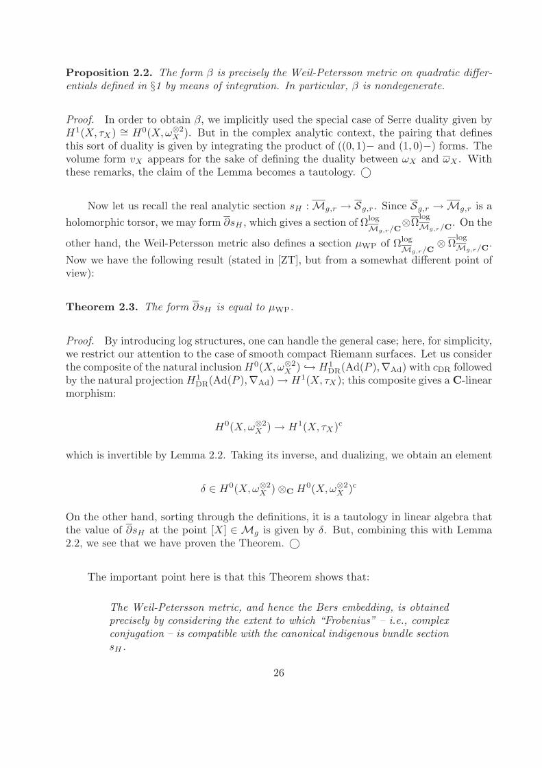
Proposition 2.2. The form β is precisely the Weil-Petersson metric on quadratic differ-entials defined in §1 by means of integration. In particular, β is nondegenerate.

Proof. In order to obtain β, we implicitly used the special case of Serre duality given byH1(X, τX) ∼= H0(X,ω⊗2

X ). But in the complex analytic context, the pairing that definesthis sort of duality is given by integrating the product of ((0, 1)− and (1, 0)−) forms. Thevolume form vX appears for the sake of defining the duality between ωX and ωX . Withthese remarks, the claim of the Lemma becomes a tautology. ©

Now let us recall the real analytic section sH : Mg,r → Sg,r. Since Sg,r → Mg,r is aholomorphic torsor, we may form ∂sH , which gives a section of Ωlog

Mg,r/C⊗Ω

log

Mg,r/C. On the

other hand, the Weil-Petersson metric also defines a section μWP of Ωlog

Mg,r/C⊗ Ω

log

Mg,r/C.

Now we have the following result (stated in [ZT], but from a somewhat different point ofview):

Theorem 2.3. The form ∂sH is equal to μWP.

Proof. By introducing log structures, one can handle the general case; here, for simplicity,we restrict our attention to the case of smooth compact Riemann surfaces. Let us considerthe composite of the natural inclusion H0(X,ω⊗2

X ) ↪→ H1DR(Ad(P ),∇Ad) with cDR followed

by the natural projection H1DR(Ad(P ),∇Ad) → H1(X, τX); this composite gives a C-linear

morphism:

H0(X,ω⊗2X ) → H1(X, τX)c

which is invertible by Lemma 2.2. Taking its inverse, and dualizing, we obtain an element

δ ∈ H0(X,ω⊗2X ) ⊗C H0(X,ω⊗2

X )c

On the other hand, sorting through the definitions, it is a tautology in linear algebra thatthe value of ∂sH at the point [X] ∈ Mg is given by δ. But, combining this with Lemma2.2, we see that we have proven the Theorem. ©

The important point here is that this Theorem shows that:

The Weil-Petersson metric, and hence the Bers embedding, is obtainedprecisely by considering the extent to which “Frobenius” – i.e., complexconjugation – is compatible with the canonical indigenous bundle sectionsH .

26

Stated in this way, the classical complex theory becomes all the more formally analogousto the p-adic theory to be discussed in this paper.

The Philosophy of Kahler Metrics as Frobenius Liftings

Before going into a detailed account of the correspondence between complex and p-adic results, we pause to explain some of the motivation for considering Kahler metrics asFrobenius liftings. Let S be a smooth p-adic formal scheme over Zp. A Frobenius lifting onS is a morphism Φ : S → S whose reduction modulo p is equal to the Frobenius morphismin characteristic p. Then the main point of the analogy is that just as (real analytic) Kahlermetrics define canonical coordinates (as discussed above), Frobenius liftings Φ : S → S(that satisfy a certain technical condition called ordinariness – see Chapter III, §1 fordetails) also define canonical coordinates, as follows:

The most basic example of an ordinary Frobenius lifting is the case when S is thep-adic completion of Zp[T, T−1] (where T is an indeterminate), and Φ−1(T ) = T p. Thenthe theory of ordinary Frobenius liftings (Chapter III, §1) states that by means of a certain“integration” procedure, every ordinary Frobenius lifting on an arbitrary S becomes (aftercompleting at a point of S) isomorphic to a product of copies of this basic example. This“integration procedure” is thus analogous to the integration procedure just reviewed whichallowed us to construct canonical coordinates associated to real analytic Kahler metrics.

The Dictionary

The fundamental “nuts and bolts” of the complex theory lies in the Beltrami equa-tion. Suppose that we think of the Beltrami equation not as a differential equation whoseunknown is the quasiconformal function fμ, but instead as an equation whose unknownis the conformal quasidisk embedding function fμ|H (in the discussion of quasidisks). Aquasidisk embedding of the universal covering space of a hyperbolic Riemann surface Xdefines an indigenous bundle (P,∇P )μ on X in a natural way. Thus, from this point ofview, we can think of the Beltrami equation as an equation whose unknown is (P,∇P )μ.Moreover, the Beltrami coefficient μ defines the “shearing” or distortion factor betweenz and z. Thus, in summary, we may regard the Beltrami equation as an equation in theunknown (P,∇P )μ in terms of the distortion factor (effected by the quasidisk embeddingfμ|H) between z and its “Frobenius conjugate” z.

On the other hand, the “nuts and bolts” of the p-adic theory lies in the study of theVerschiebung on indigenous bundles, which occupies most of Chapter II. As a functionon the indigenous bundles of a hyperbolic curve in characteristic p, the Verschiebung –which is essentially the determinant of the p-curvature – measures the distortion factorbetween applying Frobenius to an infinitesimal on the curve and applying Frobenius to aninfinitesimal motion in the (“quasidisk”) uniformization defined by the indigenous bundle.Thus, for instance, when the p-curvature is nilpotent, there is no distortion factor, and sothe indigenous bundle provides the “right” uniformization for the curve. In this sense, we

27

feel that there is an analogy between the Beltrami equation in the complex theory and theVerschiebung on indigenous bundles in the p-adic theory.

Relative to this analogy, the fundamental existence and uniqueness theorem for solu-tions to the Beltrami equation becomes the result (in Chapter II) that the Verschiebung onindigenous bundles is finite and flat. Since in the p-adic case, its degree is not one, we onlyhave uniqueness up to a finite number of possibilities. This is why we get several distinct“quasiconformal equivalence classes” in the p-adic case. Moreover, the important integraloperator “T” – i.e., the parametrix to ∂ – which gives the first term in the series expansionfor fμ may be regarded as having its analogue in the p-adic theory in the infinitesimalVerschiebung, which plays an important role throughout the paper.

More obvious is the analogy between the canonical representation ρC : π1(X) →PSL2(R) of a hyperbolic Riemann surface (arising from the upper half plane uniformiza-tion), and the canonical representation ρ∞ : Π∞ → GL±

2 (Zp) of an ordinary p-adic curve(in Theorem 0.4). Of course in the p-adic case, Π∞ has a substantial arithmetic part inaddition to its geometric part. Although generally in the complex case, there is not muchof a Galois group to work with, at least for real curves, we saw at the end of §1, that onedoes get a natural representation ρR of the full “arithmetic fundamental group” ΠR intoGL±

2 (R). Moreover, our approach to constructing ρ∞ in the p-adic case is very much akinto Bers’ approach to constructing ρC in the complex case: Namely, if one traces throughthe proof (which lies in Chapters II through V), one sees that effectively what we are doingis noting that the result is true for totally degenerate curves, and then transporting thisresult over the rest of the moduli stack of ordinary curves.

Next let us consider metrics and geometry. As we stated earlier, in some sense,one can summarize the entire complex theory by saying: We start with the hyperbolic(Kahler) metric on a hyperbolic curve, define the Weil-Petersson (Kahler) metric on themoduli stack precisely so as to be compatible with the hyperbolic metric on the curvesbeing parametrized; then our holomorphic uniformizations – i.e., both the upper half planeuniformization of the hyperbolic curve and the Bers uniformization of the moduli stack– are obtained by “integrating” the respective metrics. Similarly, the fundamental resultin the p-adic theory – namely, Theorem 0.1 – is a result about the existence of certainFrobenius liftings on the universal hyperbolic curve and its moduli stack which are uniquelycharacterized by the fact that they are compatible with each other. Here the compatibilityis expressed through the tool of the canonical indigenous bundle. Then, by “integrating”these Frobenius actions, we obtain canonical (p-adically holomorphic) coordinates (as inCorollary 0.2) on Cord and N ord

g,r . This particular analogy lies at the heart of this work.

The Bers coordinates and the coordinates of Chapter III, Theorem 2.4, are appropriatein the locus Mg,r of smooth curves. For totally degenerate curves, one has multiplicativeparameters (Chapter III, Definition 2.7) which we believe are analogous to the holomorphiccoordinates of degeneration of [Wolp], reviewed in §1. For instance, both sets of parametersare holomorphic and naturally indexed by the nodes of the totally degenerate curve.

For elliptic curves – regarded parabolically – one has, on the one hand, the well-knowntheory of the hyperbolic upper half plane, or unit disk, in the complex case, and Serre-

28

Tate theory in the p-adic case. It is interesting to note that at both types of primes(complex and p-adic), the parabolic theory may be obtained in a very precise sense asthe parabolic specializations, respectively, of Bers’ theory and of the hyperbolic p-adictheory developed in this paper. In fact, this is one of our reasons for feeling that thecanonical p-adic coordinates of Corollary 0.2 are the p-adic analogue, not of Teichmuller’scoordinates, but of Bers’: Namely, in addition to the fact that Teichmuller’s coordinates arenot holomorphic, whereas Bers’ are, Teichmuller obtains the same coordinates for 1-pointedcurves of genus 1 and parabolic elliptic curves. On the other hand, it is well-known thatBers’ coordinates are very different for 1-pointed curves of genus 1 and parabolic ellipticcurves, which is consistent with the fact that the canonical coordinates of Corollary 0.2are also very different for 1-pointed curves of genus 1 and parabolic elliptic curves.

Loose Ends

We close by saying that although, as described above, there are (what the authorbelieves to be) very strong analogies between Bers’ complex theory and the p-adic theorypresented here, the picture is by no means complete. For instance, one fundamental factin the complex case is that all r-pointed smooth curves of genus g are quasiconformallyequivalent, whereas in the p-adic case, the theory behaves as though there are severaldifferent quasiconformal equivalence classes that are permuted around to each other by acertain monodromy action in such a way that there seems to be no one quasiconformalequivalence class “which is better than the others.” Ideally, one would like to have a muchmore complete understanding of this phenomenon. In particular, one would like to knowprecisely how many quasiconformal equivalence classes there are (at least generically), aswell as a more explicit description of the set of such classes.

Also, I still do not understand what the complex, or global, analogue of a “canoni-cal p-adic curve” is. For ordinary elliptic curves, since Serre-Tate canonical liftings havecomplex multiplication, one can ask what the hyperbolic analogue of having complex mul-tiplication is. Since having complex multiplication for an elliptic curve means having lotsof isogenies, it is natural to ask if the proper hyperbolic analogue is having lots of cor-respondences, which are a sort of higher genus version of isogenies. If a hyperbolic curvedoes have a lot of correspondences, then one knows ([Marg]) that the image of its canonicalrepresentation is arithmetic. In Chapter IV, we prove that a canonical curve has lots of“pseudo-correspondences,” but unfortunately, at the time of writing, I do not see how tomake these pseudo-correspondences into genuine correspondences, so that one could applyMargulis’ result. Another issue that arises in this connection is the question of whether onecan characterize “hyperbolic curves with complex multiplication” – whatever the correctdefinition should be for this term – in terms of the Bers coordinates.

Finally, as the title implies, the present work deals exclusively with the case of ordinarycurves. In a complete theory, one would like to know what happens when one has anilpotent indigenous bundle which is not ordinary.

29

At any rate, in summary, with respect to these three issues of quasiconformal equiv-alence classes, canonical curves, and non-ordinary curves, much work remains to be done.We hope to be able to address these issues in future papers.

30

Chapter I: Crystalline Projective Structures

§0. Introduction

The purpose of this Chapter is to study the algebraic analogue of projective structureson a Riemann surface. In particular, we prove many of the analogues of results of [Gunning]in a purely algebraic framework, often making use of the crystalline site where complexanalytically one would restrict to a simply connected neighborhood on which one canintegrate. Unlike Gunning, we make systematic use of the log structures of [Kato], whichenable us to work with a very general sort of “log-curve,” that is, we can handle the caseof curves with marked points, as well as singular nodal curves on an equal footing to thesmooth case.

In §1, we discuss the notion of a Schwarz structure, which is the algebraic analogue of[Gunning]’s projective structures. We relate Schwarz structures to projective bundles withconnections as well as to square differentials, and we show that Schwarz structures naturallygive rise to a Schwarzian derivative. (Moreover, in the Appendix to this Chapter, we showthat for P1, this abstract notion of a Schwarzian derivative essentially coincides with theclassical Schwarzian derivative.) The characterizing feature of §1 is that everything takesplace locally on the curve in question. In §2, we discuss indigenous bundles (the directalgebraic analogue of [Gunning]’s indigenous bundles). What distinguishes §2 from §1 isthat in §2, we work mainly over stable curves, and thus global issues on the curve comeinto play. In §2, we are still working locally, however, on the base. In §3, we performvarious intersection theory calculations that allow us to prove that in most cases, theredo exist any canonical indigenous bundles on the universal smooth curve over a modulistack. Thus, in §3, we are concerned with issues that are global not only on the curve, butalso on the base. It should be said that all the material in this Chapter is, in some sense,“well-known,” but I do not know of any modern reference that does things from this pointof view. In particular, all the references that I know of (with the exception of [Ih], whichis algebraic, but somewhat different in point of view) discuss things only in the complexanalytic case, and often work with “hαβ’s” (i.e., cocycle classes) rather than with objectsthat have an intrinsic meaning.

§1. Schwarz Structures

In this Section, we introduce the crystalline analogue of what Gunning calls “projectivestructures on a Riemann surface.” (We shall call them Schwarz structures (after theSchwarzian derivative) to distinguish them from the analytic notion.) We begin by lettingS be a connected noetherian scheme. Often, we shall prove results about arbitrary stablecurves by working on various compactified moduli stacks. Thus, even if one is ultimatelyinterested only in smooth curves, for certain proofs, we shall see that it is useful to develop

31

the machinery for arbitrary stable curves. To deal with singular curves, we shall use thetheory of log schemes of [Kato]. Thus, we assume that S has a given fine ([Kato], §2) logstructure, and denote the resulting log scheme by Slog.

Notation and Basic Definitions

Definition 1.1. Let f log : U log → Slog be a morphism of log schemes whose underlyingmorphism of schemes f : U → S is of finite type, flat and of relative dimension one. Thenwe shall say that f log is locally stable of dimension one if, for every point u ∈ U , thereexist etale morphisms T → S and V → U ×S T , together with v ∈ V mapping to u ∈ Usuch that when we pull-back the log structure on S (respectively, U) to T (respectively,V ) to obtain log schemes V log and T log, one of the following holds:

(1) V → T is smooth, and V log = V ×T T log (where V and T denote thelog schemes with trivial log structure); or

(2) V → T is smooth, and there exists a section s : T → V such that if wedenote by V s the log scheme defined by the relative divisor Im(s) on V ,then V log = V s ×T T log; or

(3) let Y = Spec(Z[t]); X = Y [x, y]/(xy− t) (where x, y, and t are indeter-minates) and endow Y (respectively, X) with the log structure arisingfrom the divisor t = 0 (respectively, xy = 0), so we get a morphismX log → Y log of log schemes; then there exists a morphism of log schemesT log → Y log, together with a morphism ζ log : V log → T log ×Y log X log

such that the underlying scheme morphism ζ of ζ log is etale, and thelog structure of V log on V is the pull-back via ζ of the log structure onT log ×Y log X log.

In case (1) (respectively, (2); (3)), we shall say that f is smooth and unmarked (respectively,marked; singular) at u.

Note that if f log : U log → Slog is locally stable of dimension one, then it is always logsmooth ([Kato], §3). Also, note that by etale descent, the images in U of all the sectionss as in Case (2) above form a divisor in U which is etale over S. We shall refer to thisdivisor as the divisor of marked points in U .

Now let us suppose that there exists an odd prime p which is nilpotent on S. We alsosuppose that we are given a closed subscheme S0 = V (I) ⊆ S, where the sheaf of idealsI has a divided power structure γ. We denote the log scheme S0 ×S Slog (where S0 andS denote the log schemes which are the respective schemes endowed with the trivial logstructure) by Slog

0 . Let f log : U log → Slog be locally stable of dimension one. Then weshall call a section of DΔ(U log ×Slog U log) (the PD-envelope of the diagonal, as in [Kato],

32

§5) a bianalytic function over U log. Note that the bianalytic functions form a sheaf, whichwe denote OUbi , on the etale site of U . Let OU denote the sheaf on the etale site of Ugiven by considering ordinary functions. Then the two projections U ×S U → U give riseto injections iL : OU → OUbi and iR : OU → OUbi whose images we shall call the left-sided(respectively, right-sided) bianalytic functions on U log. We shall also refer to right-sidedbianalytic functions as constant bianalytic functions, or bianalytic constants. We denotetensor products of an OU -module F over OU with OUbi via iL (respectively, iR) by writingF on the left (respectively, right). Finally, we have a multiplication morphism μ : OUbi →OU . We denote the ideal subsheaf of OUbi which is the kernel of μ by J . We shall saythat a bianalytic function f over some etale V → U is a bianalytic uniformizer on V if fis, in fact, a section of J which generates the line bundle J /J [2] ∼= ωU log/Slog as an OU -module. Let OUbi be the completion of OUbi with respect to the divided powers J [i], andlet J ⊆ OUbi be the closure of J in OUbi . We shall call sections of OUbi biformal functions,and use similar terminology for biformal functions as we do for bianalytic functions.

Occasionally, we shall also need to make use of trianalytic (respectively, triformal)functions, i.e., sections of DΔ(U log ×Slog U log ×Slog U log) (respectively, its completion withrespect to the divided powers of the diagonal ideal). We denote the sheaf of trianalyticfunctions (respectively, triformal) on the etale site of U by OUtr (respectively, OUtr), andwe have left, right, and middle injections j1, j2, j3 : OU → OUtr , as well as injectionsj12, j23, j13 : OUbi → OUtr . We shall apply similar terminology and notation to trianalyticor triformal functions to that applied already to bianalytic functions. In particular, weshall call trianalytic functions that are in the image of j23 trianalytic constants.

Definition 1.2. Let S ⊆ OUbi be a subsheaf in the category of sets. We shall call S aSchwarz (respectively, pre-Schwarz) structure on U log if etale locally on U (i.e., for someetale cover V → U), S has the following form: there exists some biformal uniformizerz ∈ Γ(V,S) such that for every etale W → V , and every section f ∈ Γ(W,OUbi), thenf ∈ Γ(W,S) if and only if (respectively, implies that) f can be written etale locally (on W )in the form (az + b)/(cz + d), where a, b, c, d are biformal constants and d is invertible.

It is clear that if S ⊆ OUbi is a pre-Schwarz structure on U log, then S is contained in aunique Schwarz structure Sa ⊆ OUbi on U log, which we refer to as the Schwarz structureassociated to S. If S is a Schwarz structure, then we shall denote by S× ⊆ S (respectively,LS) the subsheaf consisting locally of functions of the form (az+b)/(cz+d), where: (1) z is

a biformal uniformizer belonging to S; (2) d is invertible; and (3)

(a b

c d

)is an invertible

matrix of biformal constants (respectively, b = 0). We let L×S = LS

⋂S×. Thus S×, LS ,and L×

S are all pre-Schwarz structures. We shall call L×S (respectively, LS) the sheaf of

biformal uniformizers (respectively, pseudo-uniformizers) of S.

Let G → U be the group scheme PGL2, and let B ⊆ G be the subgroup scheme whichis the standard Borel subgroup of PGL2, i.e., the image of the lower triangular matrices.

33

First Properties of Schwarz Structures

Proposition 1.3. The subsheaf L×S ⊆ S consisting of biformal uniformizers of S forms a

B-torsor BS → U .

Proof. This follows immediately from the definition of a Schwarz structure. The action of

B is given by associating to a biformal uniformizer z and a matrix

(a 0

c d

)(where a, c, d

are biformal constants, and a, d are invertible) the biformal uniformizer az/(cz + d). ©

Note that every B-torsor T → U naturally defines a P1-bundle with a given section (bytaking the quotient of P1 ×U T modulo the diagonal action of B, where B acts on P1 bymeans of affine transformations that fix zero; the section is the image of the zero sectionof P1). We shall refer to the P1-bundle PS → U associated to BS → U as the P1-bundleassociated to the Schwarz structure S. We denote by σS : U → PS the natural section(arising from the fact that the structure group is B rather than G).

Proposition 1.4. Let S be a Schwarz structure on U log. Then PS ∼= P(J /J [3]), andσ∗SτPS/U

∼= (J /J [2])∨ ∼= τU log/Slog . In particular, if U → S is proper, then the height ofσS with respect to τPS/U is −deg(ωU log/Slog).

Proof. One sees by construction (e.g., by writing out transition functions) that the sheaf ofnonzero relative rational functions of relative degree one (as in [EGA IV], §20) for PS → Uthat vanish at σ is naturally isomorphic to L×

S . Thus, by considering Taylor expansionsout to second order terms, we get an isomorphism OPS (−σS)/OPS (−3σS) ∼= J /J [3] (herewe use that p is odd). On the other hand, by multiplying and then taking the residue atσ, we obtain a natural duality between OPS (−σS)/OPS (−3σS) and π∗ωPS/U (3σS), whereπ : PS → U is the natural projection. Also, note that via this duality, the filtration inducedby π∗ωPS/U (2σS) ⊆ π∗ωPS/U (3σS) on OPS (−σS)/OPS (−3σS) is the filtration defined bythe submodule OPS (−2σS)/OPS (−3σS). Since PS is clearly naturally isomorphic to theprojectivization of π∗ωPS/U (3σS), we thus obtain the result. ©

Crystalline Schwarz Structures and Monodromy

Let S be a Schwarz structure on U log. We would like to associate to S a subsheaf (inthe category of sets) of OUtr , which we shall call S12 as follows. We work locally. Thus,we assume that there exists a biformal uniformizer z ∈ Γ(U,S). We consider the triformalfunction z12 defined by j12(z), where j12 is the natural map OUbi → OUtr given by inclusionon the first two factors. Then we let S12 be the sheaf of all functions which etale locallycan be written in the form (az12 + b)/(cz12 + d), where a, b, c, d are triformal constantsand d is invertible. Note that the definition of S12 does not depend on the choice of z,

34

so everything glues together, and we obtain the subsheaf S12 of OUtr over our original U .On the other hand, we also have a subsheaf S13 of OUtr defined in the same way as S12,except with the roles of 2 and 3 reversed.

Definition 1.5. We shall say that the Schwarz structure S is a crystalline Schwarzstructure on U log if the two subsheaves S12 and S13 of OUtr coincide. Let S be a crystallineSchwarz structure on U log. Then we shall say that S has nilpotent monodromy if for everymarked point s : T → V (with V → U etale), there exists a biformal uniformizer z ∈ S(V )and a section a ∈ ωU log/Slog(V ) such that the image of (dz) − iR(a) (where “d” is theexterior derivative on the right) in OUbi ⊗OU

s∗ωU log/Slog is zero.

Remark. Of course, one may also phrase the definition of a crystalline Schwarz structureas follows. First, note that OUbi , together with its right-hand sided OU -algebra structureand standard logarithmic connection, forms a quasi-coherent crystal of algebras A on thecrystalline site of U log/Slog. Then a crystalline Schwarz structure is a subsheaf of the sheafA on the crystalline site of U log/Slog satisfying certain properties. Since this point of viewis only formally different from the point of view of Definition 1.5, we shall use these twopoints of view interchangeably in what follows.

Let us suppose that S is a Schwarz structure on U log. Let H ⊆ G be the open

subscheme consisting of matrices of the form

(a b

c d

), where d is invertible. Note that

H is stable under the action by B from the right. Thus, we can take the quotient ofH ×U BS (by the diagonal action of B) to obtain a fiber bundle HS → U with fiberslocally isomorphic to H → U . Similarly, we also obtain a G-torsor GS → U . It nowfollows immediately from the definitions that the sheaf defined on the etale site of U byHS is naturally isomorphic to S×. Thus, if we assume that the Schwarz structure Sis crystalline, we see that we get a natural isomorphism between the two pull-backs ofHS → U via iL, iR : OU → OUbi , i.e., we get a logarithmic connection ∇HS on HS → U .By basic facts about fiber bundles, this gives a logarithmic connection ∇GS on GS → U anda logarithmic connection ∇PS on PS → U , as well. Thus, in summary, to every crystallineSchwarz structure S, we have associated a natural P1-bundle with section and logarithmicconnection (PS → U ;σS : U → PS ;∇PS ). Moreover, it follows from the definition ofthe connection ∇PS that by differentiating σS by means of ∇PS , we get an isomorphismτU log/Slog ∼= σ∗

SτPS/U , which is called the Kodaira-Spencer morphism. Indeed, to see thatthis morphism is, indeed, an isomorphism, it suffices to realize that if, locally on U , onetakes a biformal uniformizer z, the difference j12(z) − j13(z) generates j23(J )OUtr .

In addition to the fact that the Kodaira-Spencer morphism is an isomorphism, thelogarithmic connection ∇PS has another special property: If S has nilpotent monodromy,then we can make more explicit the way in which this monodromy acts. Indeed, letus recall from [Kato], §6, that if s : S → U is any marked point, then there exists aunique subsheaf Ms of (OUbi⊗OU ,s−1OS)/OS which is isomorphic to OS and annihilatedby the monodromy operator of the standard logarithmic connection on OUbi . (Locally,

35

this subsheaf is generated by log(1− δ), where δ = 1− (1⊗tt⊗1 ), and t is a local generator of

the ideal defining s.) This subsheaf Ms thus defines a section qs : S → P(J /J [3]) thatlies over s. Then it follows from these observations, plus Proposition 1.4, that

Proposition 1.6. If S is a crystalline Schwarz structure on U log with nilpotent mon-odromy, then under the isomorphism PS ∼= P(J /J [3]) of Proposition 1.4, qs is fixed bythe monodromy action on PS ∼= P(J /J [3]) at s.

Correspondence with P1-bundles

So far, from a crystalline Schwarz structure, we have constructed a P1-bundle withsection and logarithmic connection (satisfying certain properties). We can go the otherway, as well. Suppose we are given a P1-bundle with section and logarithmic connection(π : P → U ;σ : U → P ;∇P ) such that the Kodaira-Spencer morphism obtained bydifferentiating σ via ∇P gives an isomorphism τU log/Slog ∼= σ∗τP/U . Let PL and PR denotethe pull-backs of π : P → U via iL, iR : OU → OUbi , respectively. Then the connection ∇P

defines an OUbi-linear isomorphism Ξ : PL ∼= PR. Thus, we have a commutative diagram:

PL Ξ−→ PR⏐⏐�πL

⏐⏐�πR

Ubi id−→ Ubi

Let σL (respectively, σR) denote the result of base-changing σ via iL (respectively, iR).Then by applying (σL)∗, we can pull-back functions on PL to biformal functions on U log.Let R denote the etale sheaf of degree ≤ 1 relative rational functions (as in [EGA IV],§20) on P relative to π : P → U (i.e., the divisor of poles is flat of degree ≤ 1 over U)that are regular in a neighborhood of the image of σ. Let αR : PR → P denote thenatural projection. Then it is easy to see that Ξ−1(αR)−1(R) defines a sheaf of functionson PL that are regular in a neighborhood of Im(σL), so we can consider the subsheaf Sof biformal functions on U log which is the image of (σL)−1Ξ−1(αR)−1(R). One checksimmediately that S defines a Schwarz structure, and, moreover, that since the connection∇P is necessarily integrable (since the dimension of U over S is one), S is automaticallycrystalline. Thus, in summary, we have the crystalline analogue of Theorem 2 of [Gunning]:

Theorem 1.7. If f : U → S is as above, then there is a natural one-to-one correspondencebetween crystalline Schwarz structures on U log and isomorphism classes of P1-bundles withsection and logarithmic connection (π : P → U ;σ : U → P ;∇P ) on U log whose associatedKodaira-Spencer morphism is an isomorphism. Moreover, under this correspondence, thecrystalline Schwarz structures with nilpotent monodromy correpond precisely to the triplessuch that ∇P has nilpotent monodromy at the marked points.

36

Proof. We have already defined maps going in either direction. Thus, it suffices to seethat these maps are inverse to each other. Now it is easy to see that if we start witha P1-bundle with section and logarithmic connection as above, construct the associatedcrystalline Schwarz structure S, and then from that the associated P1-bundle PS withsection σS and logarithmic connection ∇PS , then we get back our original data. Thus, itsuffices to show that the map that associates a P1-bundle with section and connection toa crystalline Schwarz structure is injective.

Let S and S ′ be crystalline Schwarz structures on U log. Suppose that we are givena horizontal isomorphism α between PS and PS′ that takes σS to σS′ . Then α inducesan isomorphism αB of the B-torsors BS and BS′ . Let A be the OU -algebra OUbi viathe morphism iR. Since as sheaves with B-action, BS ∼= L×

S and BS′ ∼= L×S′ , we get an

isomorphism αL : L×S → L×

S′ , which, by mapping a biformal uniformizer z ∈ Γ(U,L×S )

(where U → X is etale) to the biformal uniformizer αL(z) ∈ Γ(U,L×S′) ⊆ Γ(U,A), defines

an automorphism αA of the PD-OU -algebra A that preserves the augmentation μ : A →OU . Moreover, it follows from the horizontality of α that αA is horizontal with respectto the standard logarithmic connection on A. On the other hand, it is immediate that Adoes admit any nontrivial horizontal automorphisms (as a PD-OU -algebra) that preserveμ. Thus, αA is the identity, and hence, S and S ′ must be the same subsheaf of A. Thiscompletes the proof of the first statement. The last statement follows directly from thedefinitions. ©

Schwarz Structures and Square Differentials

We would like to use Theorem 1.7 to exhibit the space of Schwarz structures as atorsor over the square differentials. Let π : P → U be a P1-bundle. Then we shall denoteby Ad(P ) the vector bundle on U (of rank three with trivial determinant) given by π∗τP/U .When we consider marked points, it is not enough just to deal with P1-bundles; we mustdeal with P1-bundles equipped with parabolic structures, as in [Sesh]. Thus, if our divisorD of marked points is given by sections p1, . . . , pr : S → U , we make the following

Definition 1.8. A P1-bundle with parabolic structure on U log is defined to be a P1-bundleπ : P → U , together with sections qi : S → P lying over pi. A rank two vector bundlewith parabolic structure on U log is a rank two vector bundle E , together with a parabolicstructure on P(E).

Let (π : P → U ; q1, . . . , qr) be a P1-bundle with parabolic structure on U log. Thenwe define the subsheaf Adq(P ) ⊆ Ad(P ) to be the sheaf of sections that vanish at theqi’s. We define Adc(P ) ⊆ Adq(P ) to be the subsheaf of sections that vanish to secondorder (in the relative coordinate for π) at the qi’s. Suppose that we are given a sectionσ : U → P that avoids all the qi. Let L = σ∗ωP/U . Then Ad(P ) gets a filtration0 = F 2(Ad(P )) ⊆ F 1(Ad(P )) ⊆ F 0(Ad(P )) ⊆ F−1(Ad(P )) = Ad(P ) given by consideringsections of τP/U that vanish to first or second order at σ. Thus, for Ad(P ), we have:

37

F 1 ∼= L; F 0/F 1 ∼= OU ; F−1/F 0 ∼= L−1

This filtration induces filtrations on Adq(P ) and Adc(P ). The subquotients are easily seento be the following: For Adq(P ), we have:

F 1 ∼= L(−D); F 0/F 1 ∼= OU ; F−1/F 0 ∼= L−1

For Adc(P ), we have:

F 1 ∼= L(−D); F 0/F 1 ∼= OU (−D); F−1/F 0 ∼= L−1

Often, L ∼= ωlogU/S . Thus, for computational purposes, it is convenient to note that

ωlogU/S(−D) is none other than the relative dualizing sheaf of the morphism f : U → S.

Now let us assume that π : P → U is given by P(J /J [3]), with the section σ givenby J /J [3] → J /J [2], and the qi given by the sections “qs” defined in the paragraphpreceding Proposition 1.6. Let ∇P be a logarithmic connection whose Kodaira-Spencermorphism at σ is the identity and whose monodromy at the marked points is nilpotentand fixes the qi. (It is not difficult to see that such ∇P always exist etale locally on U .)Then any other such logarithmic connection ∇′

P on P → U is given by adding to ∇P asection of F 0(Adc(P )) ⊗OU

ωlogU/S . On the other hand, the quadruples (π;σ; qi;∇P ) and

(π;σ; qi;∇′P ) are isomorphic if and only if ∇′

P can be obtained from ∇P by applying anautomorphism α of (π;σ; qi) that preserves the conormal bundle to σ (since both Kodaira-Spencer morphisms are the identity). Such an automorphism α is given by a sectionof F 1(Adq(P )). The effect of such an automorphism α on the connection ∇P is givenby adding to ∇P the section of Adc(P ) ⊗OU

ωlogU/S obtained by applying the morphism

Ad(∇P ) : F 1(Adq(P )) → F 0(Adc(P )) ⊗OUωlog

U/S (induced by the connection ∇P ) toα. Thus, we obtain that the set of isomorphism classes of quadruples (π;σ; qi;∇P ) that,relative to the bijection of Theorem 1.7, correspond to crystalline Schwarz structures withnilpotent monodromy are a torsor over the cokernel of Ad(∇P ). On the other hand, bylooking at the explicit representations of the subquotients of the filtrations on Adq(P ) andAdc(P ) (given in the preceding paragraph), and using the fact that the Kodaira-Spencermorphism for ∇P at σ is an isomorphism, we obtain that

Coker(Ad(∇P )) ∼= (ωlogU/S)⊗2(−D)

(We remark that here one uses the fact that p is odd, for when one computes Ad(∇P ) from∇P , certain factors of 2 appear, and in order to get the above isomorphism, one needs forthose factors of 2 to be invertible.)

In other words, we have proven the following result:

38

Theorem 1.9. The etale sheaf of crystalline Schwarz structures on U log with nilpotentmonodromy is naturally a torsor over the sheaf (ωlog

U/S)⊗2(−D).

Normalized P1-bundles with Connection

Let us consider the P1-bundle π : P = P(J /J [3]) → U , and section σ : U → Pgiven by J /J [3] → J /J [2], without any connection. Now, just as in the proof of Propo-sition 1.4, by taking residues, we obtain a natural duality between OP (−σ)/OP (−3σ)and π∗ωP/U (3σ) that respects the natural filtrations on the two bundles. Let Q =P((J /J [3])∨). As U -schemes, we may identify Q and P . Let OQ(1) denote the linebundle obtained from the definition of the projectivization; thus π∗OQ(1) = (J /J [3])∨.Let L = π∗{OQ(1)⊗OQ

τP/U (−3σ)}. Then L is a line bundle on U and (J /J [3])∨ = L⊗OU

π∗ωP/U (3σ). Thus, we obtain a natural isomorphism OP (−σ)/OP (−3σ) ∼= (J /J [3])⊗OUL

that respects filtrations. If we then look at the quotients of both sides by their respectiverank one subbundles (that make up the filtrations), we obtain an isomorphism betweenωlog

U/S∼= OP (−σ)/OP (−2σ) ∼= (J /J [2])⊗L ∼= ωlog

U/S ⊗L. That is, we get a natural trivial-ization OU

∼= L of L. In summary, we see that without any connection, we have constructeda natural filtration-preserving isomorphism:

γ : OP (−σ)/OP (−3σ) ∼= J /J [3]

Now let us suppose that we have a logarithmic connection ∇P on π whose Kodaira-Spencer morphism at σ is an isomorphism. Then we get a commutative diagram like theone preceding Theorem 1.7. Pulling back by αR, then Ξ, and finally by σL, we thus seethat ∇P induces an isomorphism:

ζ(∇P ) : OP (−σ)/OP (−3σ) ∼= J /J [3]

Now we saw above (Theorem 1.7) that ∇P defines a Schwarz structure. But one “looseend” relative to the statement of Theorem 1.7 is that although Schwarz structures have noautomorphisms, triples consisting of projective bundles with a section and a connection canhave automorphisms. These automorphisms were the cause of the phenomenon (observedjust before the statement of Theorem 1.9) that many different ∇P can give rise to the sameSchwarz structure. Thus, it is convenient to have some sort of notion of a “normalized∇P ” such that each Schwarz structure arises from a unique normalized ∇P . We choosethe normalization as follows:

Definition 1.10. We say that ∇P is normalized if γ and ζ(∇P ) are inverse to eachother.

Now as a formal consequence of this definition, we observe that we obtain the followingnormalized version of Theorem 1.7:

39

Theorem 1.11. If f : U → S is as above, then there is a natural one-to-one correspon-dence between crystalline Schwarz structures on U log and normalized logarithmic connec-tions on the P1-bundle π : P(J /J [3]) → U whose associated Kodaira-Spencer morphismat the section σ : U → P (defined by J /J [3] → J /J [2]) is an isomorphism. Moreover,under this correspondence, the crystalline Schwarz structures with nilpotent monodromycorrepond precisely to the triples such that ∇P has nilpotent monodromy at the markedpoints.

The Schwarzian Derivative

Before proceeding, it is interesting to note that, as the name suggests, a crystallineSchwarz structure S allows one to define a Schwarzian derivative dS , as follows. Letω×

U log/Slog ⊆ ωU log/Slog denote the subsheaf consisting of sections that locally generate

ωU log/Slog as an OU -module. Let O#U ⊆ OU be the subsheaf consisting of functions φ such

that dφ is a section of ω×U log/Slog ⊆ ωU log/Slog . Then our Schwarzian derivative will be a

morphism of sheaves of sets:

dS : O#U → ω⊗2

U log/Slog

Let θ be a section of O#U over some etale V → U . Let us denote by jθ ∈ J /J [3](V ) the 2-

jet of θ (i.e., the Taylor expansion out to second order, modulo the constant term). By thedefinition of O#

U , the image of jθ in J /J [2](V ) is a local generator of the sheaf J /J [2]. ByProposition 1.6, jθ then defines a section sθ : V → PS . Taking the Kodaira-Spencer mapof this section then defines an OV -linear morphism from τU log/Slog to the conormal bundleto sθ, which is simply ωU log/Slog . This OV -linear morphism is thus given by multiplicationby a section of ω⊗2

U log/Slog , which we take to be dS(θ). A simple calculation reveals that

Proposition 1.12. If (as in Theorem 1.9) one modifies the Schwarz structure S byadding the square differential δ ∈ [(ωlog

U/S)⊗2(−D)](U) to obtain a Schwarz structure S ′,then dS(θ) = dS′(θ) + δ.

We also have a biformal version of the Schwarzian derivative. Namely, we let O#

Ubibe

the subsheaf of OUbi consisting of biformal functions φ that are of the form u + c, where uis a biformal uniformizer, and c is a biformal constant. Then we get a morphism of sheavesof sets:

dbiS : O#

Ubi→ (ω⊗2

U log/Slog)Ldef= ω⊗2

U log/Slog ⊗OUOUbi

defined as follows: If θ is a section of O#

Ubiover some etale V → U , we let jθ be the

section of J /J [3] ⊗OUOUbi which is the 2-jet of θ. Thus, jθ defines a section of sθ of PL

S

40

whose Kodaira-Spencer map is given by multiplication by a section of (ω⊗2U log/Slog)L, which

we take as dbiS (θ). Note that dbi

S (iL(θ)) = iL(dS(θ)), and that if we modify the Schwarzstructure by adding a square differential δ, then

dbiS (θ) = dbi

S′(θ) + iL(δ)

Remark. In the Appendix to this Chapter, we show that the definition just given for theSchwarzian derivative coincides with one-half the classical Schwarzian derivative, when Uis the projective line.

For the biformal version of the Schwarzian, we have an analogue of the classicalresult that the Schwarzian vanishes exactly on the formal functions that make up theprojective structure of a Riemann surface. Indeed, let Ξ : PL

S → PRS be the isomorphism

defined by the connection ∇PS ; let αR : PRS → PS be the natural projection; and let

ζ : Ubi def= Spec(OUbi) → PS be the morphism obtained by composing σLS : Ubi → PL

S withΞ and then αR. Since the definition of dS is functorial, dS applied to a function pulled backby ζ is ζ−1 of the “dS” computed for projective bundles in the Appendix, i.e., one-half theclassical Schwarzian. Thus, if θ is a section of S, then θ is the pull-back by ζ of a (degree≤ 1) relative rational function for PS → U , so dbi

S (θ) = 0.

Conversely, suppose that dbiS (θ) = 0. Then the statement that dbi

S (θ) = 0 meansthat sθ is a horizontal section of PL

S . Thus it follows from the definition of a connection,together with the Poincare Lemma in crystalline cohomology (see, e.g., [Kato], §6 for thelog version) that Ξ(sθ) is the pull-back via αR of a section tθ of PS . Now (after possibleetale localization), we can find a (degree ≤ 1) relative rational function φ for PS → U

whose 2-jet at σS is given by the section tθ. Since ζ maps the diagonal in Ubi to σRS , and

the formation of 2-jets is functorial, it thus follows that the 2-jet of ψdef= ζ−1(φ) defines

a section sψ of PLS which is equal to sθ when restricted to the diagonal U ⊆ Ubi. But

since both sψ and sθ are horizontal, they must be equal. The biformal functions ψ andθ thus have 2-jets that define the same “line” in J /J [3]. Let z be a local coordinate onU . Let us denote by successive primes the derivatives of biformal functions (i.e., taken onthe left) with respect to z. Then we obtain that ψ′ and θ′ are both invertible biformalfunctions such that ψ′′ · θ′ = ψ′ · θ′′. It thus follows that (ψ′/θ′)′ = 0, so θ′ = a ψ′, wherea is an invertible biformal constant. Thus, θ = a ψ + b, where b is a biformal constant.Since, by construction ψ ∈ S(V ), it follows that θ ∈ S(V ). Thus, we obtain the following“crystalline Schwarzian Poincare Lemma:”

Theorem 1.13. If θ is a biformal function, then dbiS (θ) = 0 if and only if θ is a section

of S.

41

§2. Indigenous Bundles

In this Section, we globalize the local considerations of §1, and are thus led to introduce“indigenous bundles” (as in [Gunning]). Let Slog be a fine log scheme, whose underlyingscheme is connected noetherian. Let f log : X log → Slog be proper, geometrically connected,and locally stable of dimension one. (Note that the first two conditions are actuallyconditions on the underlying scheme morphism f .) We assume that the fibers of f : X → Shave arithmetic genus g ≥ 0, and exactly r ≥ 0 marked points (as in Definition 1.1 – notethat these may only be defined etale locally, however).

Basic Definitions and Examples

If 2g − 2 + r ≥ 1, then let Mg,r be the moduli stack of stable curves of genus g,with r marked points, over Z, and let ζ : C → Mg,r be the universal curve, with its rmarked points s1, . . . , sr : Mg,r → C. Note that Mg,r has a natural log structure givenby the divisor at infinity. Denote the resulting log stack Mlog

g,r. Also, by taking the divisorwhich is union of the si and the pull-back of the divisor at infinity of Mg,r, we get a logstructure on C; we call the resulting log stack Clog. Also, ζ : C → Mg,r extends naturallyto a morphism of log stacks ζ log : Clog → Mlog

g,r.

Definition 2.1. We shall say that f log : X log → Slog is stable if there exists a classifyingmorphism φlog : Slog → Mlog

g,r such that X log ∼= Slog ×Mlogg,r

Clog.

Ultimately, we shall be concerned mainly with the case where f log is stable, but it is usefulto realize that the definition, as well as many of the first properties, of indigenous bundlescan be made without these assumptions.

Let π : P → X be a P1-bundle. If σ : X → P is a section, then we call the canonicalheight of σ the number 1

2degX/S(σ∗τP/X), where degX/S denotes the relative degree over Sof a line bundle on X, and τP/X is the relative tangent bundle of π. If ∇P is a logarithmicconnection on P , then we call the morphism τXlog/Slog → σ∗τP/X given by differentiatingσ by means of ∇P the Kodaira-Spencer morphism at σ relative to ∇P . Often, instead ofdealing with P1-bundles with logarithmic connections, it will be more convenient to dealvector bundles: Thus, let E be a vector bundle equipped with a logarithmic connection∇E , whose rank is two and whose determinant is trivial. Then Theorem 1.7 motivates thefollowing

Definition 2.2. We shall say that (π : P → X,∇P ) is an indigenous bundle on X log ifthe monodromy at the marked points (which exist etale locally) is nilpotent, and thereexists a section σ : X → P of π such that the Kodaira-Spencer morphism at σ withrespect to ∇P is an isomorphism. We shall say that (E ,∇E) is an indigenous vector bundle

42

on X log if the associated P1-bundle with logarithmic connection (P(E) → X,∇P(E)) is anindigenous P1-bundle. We shall say that P → X (respectively, E) is intrinsic if there existsa logarithmic connection ∇P (respectively, ∇E) on P → X (respectively, E) that makes(P → X,∇P ) (respectively, (E ,∇E)) indigenous. We shall say that P → X (respectively,E) is locally intrinsic if it is intrinsic etale locally on S.

Thus, in the vector bundle case, (E ,∇E) is indigenous if ∇E has nilpotent monodromyat the marked points, and there exists a rank one subbundle F 0(E) ⊆ E such that theKodaira-Spencer morphism F 0(E) → ωXlog/Slog ⊗OX

(E/F 0(E)) (induced by ∇E) is anisomorphism.

So far we have been discussing the hyperbolic case (2g − 2 + r ≥ 1); however, one canmake the same definition for curves that are not hyperbolic.

Example 1. Suppose that f : X → S is smooth, with no marked points, and thatg = 0. Thus, f is a P1-bundle. Then the P1-bundle given by X ×S X → X has a naturaltrivial connection, together with a natural section, the diagonal section. It is trivial to seethat this triple satisfies the required properties for an indigenous bundle.

Example 2. Suppose that f log : X log → Slog has no marked points, and that its fibersall have arithmetic genus one. Then consider the bundle E = ωX/S ⊕ OX (where ωX/S

is the relative dualizing sheaf). Let L = f∗ωX/S . Thus, L is a line bundle on S, andf∗L ∼= ωX/S . In particular, there exists on ωX/S a “trivial connection” ∇ω obtained fromtensoring the trivial connection on OX with f∗L. Let ∇′

E be the connection on E whichis the direct sum of ∇ω and the trivial connection on OX . Let ∇E be the connection onE given by adding to ∇′

E the section of End(E) ⊗ ωX/S given by projecting E → ωX/S∼=

(0,OX) ⊗ ωX/S ⊆ E ⊗ ωX/S . Then one checks easily that if we take (P,∇P ) = P(E ,∇E),and σ : X → P to be given by (ωX/S , 0) ⊆ E , then we obtain an indigenous bundle onX log.

Example 3. Let Slog = Spec(Z) (with the trivial log structure); X log = M1,1 (themoduli stack of one-pointed curves of genus one over Z), with its natural log structure.Let E be the vector bundle of rank two on X which is the first de Rham cohomologymodule of the universal one-pointed curve of genus one. Then E has a natural logarithmicconnection ∇E , the so-called “Gauss-Manin connection.” There is also a natural Hodgefiltration F 1(E) ⊆ E , which defines a section σ : X → P

def= P(E). The pair (E ,∇E) formsthe prototypical example of an indigenous bundle on X log.

First Properties

We now proceed to examine basic properties of such bundles.

43

Proposition 2.3. If f log : X log → Slog and hlog : Y log → Slog are as stipulated at thebeginning of the Section, and ζ log : Y log → X log is a log etale morphism of log schemesover Slog that sends marked points to marked points, then the pull-back via ζ log of anyindigenous bundle is again indigenous.

Proof. This follows from the definitions. ©

Proposition 2.4. If π : P → X is intrinsic, then the section σ : X → P is of canonicalheight 1 − g − 1

2r. If X log → Slog is a stable curve (so, in particular, 2g − 2 + r ≥ 1),then σ is the unique section of π of canonical height 1− g− 1

2r. We shall refer to σ as theHodge section of π : P → X.

Proof. The fact that the canonical height of σ is 1− g− 12r follows from the fact that the

Kodaira-Spencer morphism is an isomorphism. Now suppose that X log → Slog is stable.Let us first assume that S is the spectrum of an algebraically closed field. Suppose thatσ′ : X → P also has canonical height 1−g− 1

2r. Then it follows that its restriction to someirreducible component of X has negative canonical height. Since the restriction of σ∗τP/X

to any irreducible component has negative degree, it follows immediately from consideringintersection numbers on P , together with the definition of “canonical height,” that therecannot exist two distinct sections of negative canonical height over that irreducible com-ponent. Thus, σ and σ′ must agree over that irreducible component. Now if there areany other irreducible components in X, then σ′ must have negative canonical height oversome other irreducible component of X, in order for its canonical height over all of X tobe 1 − g − 1

2r. Thus, repeating this argument shows that σ = σ′. Finally, let us observethat the space of deformations of σ is given by H0(X,σ∗τP/X), which is zero, since σ∗τP/X

has negative degree on every irreducible component of X. The result for general S thenfollows immediately from this by deformation theory. ©

Now let us assume for the rest of the Section (unless stated otherwise) that thereexists an odd prime p which is nilpotent on S, together with a PD-ideal I ⊆ OS .

Proposition 2.5. If π : P → X is intrinsic, then P ∼= P(J /J [3]) (where J defines thediagonal in X bi). Moreover, for any connection on π that makes it indigenous, the mon-odromy at a marked point s : S → X fixes the section qs : S → P(J /J [3]) of Proposition1.6.

Proof. This follows from Theorem 1.7 and Propositions 1.3 and 1.6. Note that the secondstatement uses the fact that p is odd.©

Proposition 2.6. Suppose that the number of marked point plus nodes on any geometricirreducible component of a fiber of X → S is even. Let (π : P → X,∇P ) be indigenous on

44

X log. Then etale locally on S, there exists an indigenous vector bundle (E ,∇E) on X log

whose projectivization is (π : P → X,∇P ). Moreover, such an (E ,∇E) is unique up totensor product with a line bundle with connection (L,∇L) on X whose square is trivial.

Proof. Consider the relative anticanonical bundle τP/X on P . By Proposition 2.5, (afteretale localization on S) there exists a line bundle G on P whose square is τP/X . Nowlet us note that since the construction of the anticanonical bundle is canonical, it followsthat the connection ∇P on the P1-bundle induces a connection on the polarized P1-bundle(π : P → X, τP/X). Moreover, since the “moduli space” of line bundles G whose squareis τP/X is etale over X, it follows that the connection ∇P on the P1-bundle π : P → Xin fact induces a connection on the polarized P1-bundle (π : P → X,G). Thus, weget a connection ∇E on E def= π∗G. Moreover, on P , we have a natural exact sequence0 → ωP/X → (π∗E) ⊗ G−1 → OP → 0, which induces an isomorphism det(π∗E) ∼= OP ,hence an isomorphism det(E) ∼= OX , which is easily seen to be horizontal. Finally, it isclear that the projectivization of (E ,∇E) is isomorphic to (π : P → X,∇P ).

Now suppose that both (E ,∇E) and (E ′,∇E′) have the same projectivization (π : P →X,∇P ). Then E defines a line bundle G on P whose square is τP/X and such that ∇P

induces a connection on the polarized P1-bundle (π : P → X,G). Similarly, E ′ defines a linebundle G′ on P . Since we have horizontal isomorphisms G⊗2 ∼= τP/X and (G′)⊗2 ∼= τP/X ,it follows that if we let L = π∗((G′)−1⊗G), then L gets a natural connection ∇L such thatthe square of (L,∇L) is trivial. Moreover, (E ,∇E) ∼= (E ′,∇E′) ⊗ (L,∇L). This completesthe proof. ©

In summary, the above Proposition tells us that (under the evenness assumption) up toetale localization on the base, it is essentially the same thing to give an indigenous P1-bundle or an indigenous vector bundle. Thus, in the future, we shall frequently simplyspeak of “indigenous bundles.” The same goes for intrinsic bundles.

Existence and de Rham Cohomology

The next step is to prove the existence of indigenous bundles, and to parametrizethem. We begin with the proof of existence. For the rest of this Section, we shall assumethat f log is stable. Thus, in particular, 2g − 2 + r ≥ 1.

Theorem 2.7. For any r-pointed stable curve X log → Slog of genus g, the P1-bundleP(J /J [3]) is locally intrinsic.

Proof. From Theorem 1.9, we know that the obstruction to the existence of a crystallineSchwarz structure with nilpotent monodromy on X log (locally on S) is given by a sectionof R1f∗(ω

logX/S)⊗2(−D) over S. On the other hand, by Serre duality, R1f∗(ω

logX/S)⊗2(−D)

45

is isomorphic to the dual of f∗τXlog/Slog = 0, since the curve is stable. The Theorem nowfollows form Proposition 1.6 and Theorem 1.7. ©

Next we wish to compute the de Rham cohomology of the P1-bundle with parabolicstructure (π; qi). Note that the exterior differential operator maps Ad(P ) (respectively,Adq(P )) into Adq(P ) (respectively, Adc(P )). We define the parabolic de Rham cohomology(respectively, with compact supports) of Ad(P ) to be the hypercohomology of the complexAd(P ) → Adq(P ) ⊗ ωlog

X/S (respectively, Adq(P ) → Adc(P ) ⊗ ωlogX/S).

Theorem 2.8. Let (P,∇P ) be an indigenous bundle on an r-pointed stable curve f log :X log → Slog of genus g. Then the de Rham cohomology of Ad(P ) with its natural connec-tion (induced by ∇P ) is as follows:

(1) For cohomology without compact supports, we have (fDR)∗(Ad(P )) =R2(fDR)∗(Ad(P )) = 0; and we have a natural exact sequence

0 → f∗(ωlogX/S)⊗2(−D) → R1(fDR)∗(Ad(P )) → R1f∗τXlog/Slog → 0

(2) For cohomology with compact supports, we have (for all i ≥ 0) a naturalisomorphism

Ri(fDR)c,∗(Ad(P )) ∼= Ri(fDR)∗(Ad(P ))

In particular, (P ;∇P ) has no nontrivial automorphisms.

Proof. To compute the de Rham cohomology, one uses the long exact cohomology se-quences induced by the filtrations considered above, plus the fact that the Kodaira-Spencermorphism is an isomorphism. Now let α be an automorphism. Since (fDR)∗(Ad(P )) = 0,all infinitesimal automorphisms must vanish, so we may work over an algebraically closedfield. By passing to a tamely ramified covering of X ramified only at the marked pointsand nodes, we may assume that the hypotheses of Proposition 2.6 are satisfied. Then letL be a line bundle on P whose square is τP/X . Since L ∼= OP (σ)⊗OS

M (for a line bundleM on S), and α always preserves σ, it follows that α preserves L. Thus, α arises from ahorizontal section of End(π∗L) = OX ⊕ Ad(P ), hence is induced by multiplying π∗L by asection of OS . Thus, α is the identity, as desired. ©

Finally, combining what we have done in this Section with Theorem 1.7, we obtain:

Corollary 2.9. Let f log : X log → Slog be an r-pointed stable curve of genus g. Thenthe set of crystalline Schwarz structures on X with nilpotent monodromy is in one-to-one

46

correspondence the set of isomorphism classes of indigenous P1-bundles on X log. More-over, the functor that assigns to T log → Slog the set of crystalline Schwarz structures withnilpotent monodromy on X log

T = X log ×Slog T log is a torsor over f∗(ωlogX/S)⊗2(−D).

Indigenous Bundles of Restrictable Type

Let f logi : X log

i → Slog (for i = 1, . . . , n) be an ri-pointed smooth curve of genus gi

(where 2gi − 2 + ri ≥ 1 for all i). Suppose that we are given a graph Γ consisting of nvertices, numbered 1 through n. Let Ei be the set of edges of the ith vertex. Supposefurther that we are given an injection λi : Ei ↪→ {1, . . . , ri}. Then we can glue togetherthe curves f log

i : X logi → Slog to form an r-pointed stable curve f log : X log → Slog of genus

g in such a way that the dual graph of f log is given by Γ, that is:

(1) vertex i corresponds to f logi : X log

i → Slog, an irreducible component ofX log;

(2) if ε is an edge running from vertex i to vertex j such that λi(ε) = aand λj(ε) = b, then ε corresponds to a node on X log obtained by gluingtogether X log

i at the ath marked point to X logj at the bth marked point;

(3) g and r can be computed combinatorially from Γ, the gi’s, the ri’s andthe λi’s.

Let μlogi : X log

i ↪→ X log be the inclusion of X logi into X log as one of the irreducible

components.

Now let us suppose that we are given an indigenous bundle (π : P → X;∇P ) on X log.Then it is not necessarily the case that (μlog

i )∗(π : P → X;∇P ) will be indigenous on X logi .

The problem is that since in general, marked points of X logi might be sent to nodes of X log

(and not to marked points), there is no reason why the monodromy at such marked pointsof X log

i should be nilpotent. We therefore make the following

Definition 2.10. If the (μlogi )∗(π : P → X;∇P ) are indigenous on X log

i for all i, then wesay that (π : P → X;∇P ) is of restrictable type.

Now let us suppose that we are given indigenous bundles Πi = (πi : Pi → Xi;∇Pi)

on X logi . Note that for each marked point s : S → Xi of an X log

i , s∗Pi has a canonicaltrivialization as a P1-bundle given by considering:

(1) the Hodge section σi : Xi → Pi (pulled-back by s);

(2) the trivialization of s∗(σ∗i ωPi/Xi

) given by the residue map; and

(3) the section qs : S → s∗Pi of Proposition 1.6.

47

It thus follows that we can glue together the Πi’s by means of this canonical trivializationat the marked points to obtain an indigenous bundle Π = (π : P → X;∇P ) on X log.Moreover, by construction, Π is of restrictable type.

Also, we can clearly reverse the procedure: Namely, if we start with an indigenousbundle Π on X log of restrictable type, we can reconstruct Π by restricting to the X log

i ’s,and then regluing, in the fashion described in the preceding paragraph. Now let us define

E def=n⊕

i=1

(fi)∗ω⊗2

Xlogi

/Slog(−Di)

where Di is the divisor of marked points on Xi. Then we have the following result:

Proposition 2.11. The etale sheaf on S of isomorphism classes of indigenous P1-bundlesof restrictable type on X log is a torsor over the vector bundle E.

Note that the rank of E is given by∑n

i=1(3gi − 3 + ri), which, in general, is strictly lessthan 3g − 3 + r.

§3. The Obstruction to Global Intrinsicity

In §2, we saw that the P1-bundle P(J /J [3]) is locally intrinsic on Mg,r. In thisSection, we study the obstruction (which, in general, is nonzero) to it being globallyintrinsic over all of Mg,r. The main point is a computation in Hodge cohomology which,in many respects, is similar to that of [Falt3], Lemma IV.4. Since, however, it is notliterally the same as [Falt3], and certain technical aspects of the computation are different,we provide a complete proof here.

Introduction of Cohomology Classes

We shall work over a field K of characteristic zero, say Qp, until we state otherwise.Since we are only interested in certain intersection numbers, the base field is essentiallyirrelevant. Let us consider the universal r-pointed stable curve of genus g, ζ : C → Mg,r

(over K). We would like to consider various cohomology classes on C and Mg,r. Thecohomology theory that we will use is Hodge theory, so all cohomology classes are to beunderstood as being Hodge-theoretic. Let π : P = P(J /J [3]) → C be the P1-bundlewhich, as we saw in §2, is locally intrinsic. Let F = Ad(P ). Thus, F has a filtration whosesubquotients are given by:

F 1 ∼= L; F 0/F 1 ∼= OC; F−1/F 0 ∼= L−1

48

where L = ωClog/Mlogg,r

. Let η = c1(L), the first Chern class of L. Then we have: c1(F) = 0.

On the other hand, the second Chern class of F is given by:

c2(F) = −η2

Let us compute ζ∗η2. Let Di ⊆ C (where i = 1, . . . , r) be the marked points. LetD =

∑ri=1 Di. We shall write [Di]; [D] for the respective cohomology classes on C. Let

ξ = c1(ωC/Mg,r). Thus, η = ξ + [D]. Since different Di’s do not intersect, we have

[Di] · [Dj ] = 0 if i �= j. Also, by “taking the residue,” we see that ζ∗{(ξ + [Di]) · [Di]} = 0,for all i. Thus, ζ∗{(ξ + [D]) · [D]} = 0. Let ψi = ζ∗(ξ · [Di]); ψ =

∑ri=1 ψi; θ = ζ∗ξ2. Then

we obtain:

ζ∗η2 = ζ∗{(ξ + [D]) · ξ}

= θ + ψ

Now one knows from [AC] that for g ≥ 3, the restrictions of the classes θ and ψ to Mg,r

are linearly independent. We summarize this in a Lemma:

Lemma 3.1. We have, on Mg,r, ζ∗η2 = θ + ψ. In particular, if g ≥ 3, then (ζ∗η2)|Mg,r

is nonzero.

We shall see below that ζ∗c2(F) can be related to the obstruction to the existence of aglobal indigenous bundle on C. Thus, once we have done this, we will have proven thatthis obstruction is given by the relatively computable cohomology class −ζ∗η2 on Mg,r.

Computation of the Second Chern Class

Let us first observe that P |D has a canonical trivialization as a P1-bundle given byusing:

(1) the Hodge section σ : C → P (restricted to D);

(2) the trivialization of (σ∗ωP/C)|D given by the residue map; and

(3) the section qs : D → P ×C D of Proposition 1.6.

Let us denote by Clogc the log stack obtained by letting C be the underlying stack and

taking for the log structure the pull-back of the log structure of Mlog

g,r via ζ. Thus, we havean exact sequence on C:

0 → ζ∗ΩMlogg,r

→ ΩClogc

→ ωC/Mg,r→ 0

49

where the first two sheaves of differentials are over K. In the future, we shall think of thisexact sequence as defining a one-step filtration on ΩClog

c. For i, j ≥ 0, let us define for any

OC-module G:

Hi,jc (C,G) def= Hi(C,G ⊗OC ∧jΩClog

c)

This cohomology is a sort of cohomology with compact supports outside D. Thus, by usingthe canonical trivialization of P |D referred to above, we see that the global obstruction tothe existence of a logarithmic connection on π : P → C (for the log structure of Clog) whichhas normalized nilpotent monodromy at D defines a class κ ∈ H1,1

c (C,Ad(P )). Now, bytaking the trace of the square of κ, we get a class in tr(κ2) ∈ H2,2

c (C,OC). If we then applyζ∗, we get a class ζ∗tr(κ2) ∈ H1,1(Mlog

g,r)def= H1(Mg,r,ΩMlog

g,r

). On the other hand, let us

denote by:

Sg,r → Mg,r

the ΩMlogg,r

-torsor defined by looking at the crystalline Schwarz structures with nilpotent

monodromy on C (as in Corollary 2.9). This torsor thus defines a class Σ ∈ H1,1(Mlog

g,r).The goal of this subsection is to prove the following:

Lemma 3.2. We have the following equality of classes in H1,1(Mlog

g,r): Σ = 12ζ∗tr(κ2).

Now let us note that H1,1c (C,Ad(P )) has two one-step filtrations: one arising from

the Leray-Serre spectral sequence applied to ζ, and the other arising from the filtrationdefined above on ΩClog

c. Thinking in these terms, we see that we get a morphism:

φ00 : H1,1c (C,Ad(P )) → H0(Mg,r,R1ζ∗(Ad(P ) ⊗ ωC/Mg,r

))

Now since we know that P → C admits a connection of the desired type on the fibers of ζ,it follows that φ00(κ) = 0.

Next let us consider the natural morphism:

φ10 : H1,1c (C,Ad(P )) → H1(C,Ad(P ) ⊗ ωC/Mg,r

)

Since φ00(κ) = 0, it follows from considering the Leray-Serre spectral sequence that φ10(κ)lies in H1(Mg,r, ζ∗(Ad(P ) ⊗ ωC/Mg,r

)) ↪→ H1(C,Ad(P ) ⊗ ωC/Mg,r). In fact, by consid-

ering only normalized connections (as in Definition 1.10), we can say more. Namely, itfollows that φ10(κ) is actually the image under the morphism H1(Mg,r, ζ∗(ωClog/Mlog

g,r

⊗ωC/Mg,r

)) → H1(Mg,r, ζ∗(Ad(P ) ⊗ ωC/Mg,r)) (induced by ωClog/Mlog

g,r

↪→ Ad(P )) of the

50

class Σ (regarded as a class in H1(Mg,r, ζ∗(ωClog/Mlogg,r

⊗ωC/Mg,r)) by means of the tauto-

logical isomorphism ΩMlogg,r

∼= ζ∗(ωClog/Mlogg,r

⊗ ωC/Mg,r)).

Now let us consider the natural morphism:

φ01 : H1,1c (C,Ad(P )) → H0(Mg,r,R1ζ∗(Ad(P ) ⊗ ΩClog

c))

Since φ00(κ) = 0, it follows that the section φ01(κ) of R1ζ∗(Ad(P ) ⊗ ΩClogc

) lies in theimage of the natural map

ι : R1ζ∗(Ad(P ) ⊗ ΩMlogg,r

) → R1ζ∗(Ad(P ) ⊗ ΩClogc

)

In fact, we can say more. Since we are dealing with sheaves on Mg,r, we can computelocally on Mg,r. Let U → Mg,r be etale. Let ∇P be a logarithmic connection withnormalized nilpotent monodromy (relative to ζU : CU → U) on PU = P ×Mg,r

U . Then theobstruction to lifting ∇P to a logarithmic connection relative to CU → Spec(K) is giving bysubtracting the two pull backs of (PU → U ;∇P ) to the first infinitesimal neighborhood ΔU

of the diagonal of U ×K U . Note that it only makes sense to compare these two pull-backsbecause we have chosen a connection ∇P , so that we can deal with crystals on Crys(CU/ΔU )(where the structure morphism CU → ΔU is given by composing ζU : CU → U with thediagonal embedding U ↪→ ΔU ). Thus, the difference between the pull-backs defines asection δ (over U) of ΩMlog

g,r

|U⊗R1(ζU )DR,∗(Ad(P ),∇P ). Now if we compose the projection

R1(ζU )DR,∗(Ad(P ),∇P ) → R1(ζU )∗τClogU

/U log with δ, we get a morphism

(ΩMlogg,r

)∨|U = ΘMlogg,r

|U → R1(ζU )∗τClogU

/U log

Now it is a tautology that this morphism is none other than the isomorphism β derivedfrom deformation theory of the tangent space to Mlog

g,r with the first cohomology groupof the relative tangent bundle of ζ log. Thus, in summary, we have proven the followingstatement:

(*) locally on Mg,r, φ10(κ) is the image under ι of some local sectionν of R1ζ∗(Ad(P )⊗ΩMlog

g,r

) whose image in R1ζ∗(τClog/Mg,r)⊗ΩMlog

g,r

is

the tautological isomorphism β.

We are now ready to consider ζ∗tr(κ2). We begin by using the observations of thepreceding two paragraphs to compute what happens when we multiply various subquotientsof the two filtrations on H1,1

c (C,Ad(P )) by each other:

(1) If we multiply two elements in the image of H1(Mg,r, ζ∗(Ad(P )) ⊗ΩMlog

g,r

), and take the trace, we get a (2, 2)-Hodge cohomology class on

51

C which is the pull-back of such a class on Mg,r; thus, if we apply ζ∗ tosuch a product, we get zero.

(2) If we multiply an element in the image of H1(Mg,r, ζ∗(Ad(P ))⊗ΩMlogg,r

)

by an element in the image of H0(Mg,r,R1ζ∗(Ad(P ))⊗ΩMlogg,r

), and take

the trace, we get a class in H1(Mg,r,R1ζ∗OC ⊗ ∧2ΩMlogg,r

); since there

are no factors of ωC/Mg,rin the wedge product, applying ζ∗ again gives

zero.

(3) If we multiply two elements of H0(Mg,r,R1ζ∗(Ad(P )) ⊗ ΩMlogg,r

), we

get zero since ζ has relative dimension one.

(4) If we multiply an element in the image of H1(Mg,r, ζ∗(Ad(P ))⊗ΩMlogg,r

)

by φ10(κ) ∈ H1(Mg,r, ζ∗(Ad(P )⊗ωC/Mg,r)), and take the trace, we get

zero, since we are taking the trace of the product of a nilpotent sectionof Ad(P ) with a section of the same Borel subalgebra of Ad(P ).

(5) If we square φ10(κ) ∈ H1(Mg,r, ζ∗(Ad(P )⊗ωC/Mg,r)), we get zero since

we are, in effect, squaring nilpotent sections of Ad(P ).

(6) If we multiply φ10(κ) ∈ H1(Mg,r, ζ∗(Ad(P ) ⊗ ωC/Mg,r)) by φ01(κ) ∈

H0(Mg,r,R1ζ∗(Ad(P )⊗ΩClogc

)), then we are, in effect, multiplying theclass Σ by the tautological isomorphism β, so that we obtain Σ, regardedas a class in H1(Mg,r,ΩMlog

g,r

).

Thus, in summary, all of the possible contributions are zero, except for the last, which is2Σ. This completes the proof of Lemma 3.2. On the other hand, by basic linear algebra,c2(Ad(P )) is −2 tr(κ2), so we see that we have, in fact, proven the following:

Lemma 3.3. We have ζ∗c2(Ad(P )) = −4Σ.

Finally, putting this together with Lemma 3.1, we see that we have explicitly computedthe class Σ in terms of well-known first Chern classes of line bundles:

Theorem 3.4. The torsor of Schwarz structures defines a class Σ ∈ H1(Mg,r,ΩMlogg,r

)

which is equal to 14 (θ + ψ), where θ = ζ∗ξ2; ψ = ζ∗(ξ · [D]); ξ = c1(ωC/Mg,r

); and [D]is the cohomology class of the divisor of marked points. In particular, if g ≥ 3, then (incharacteristic zero) Sg,r → Mg,r does not admit any sections, i.e., there are no canonicalSchwarz structures on r-pointed smooth curves of genus g ≥ 3.

Remark. Ideally, it would be nice to have an equality of classes not in H1(Mg,r,ΩMlogg,r

),

but in some sort of cohomology with compact supports “H1c (Mg,r,ΩMlog

g,r

)” (which should

52

be isomorphic to H1(Mg,r,ΩMg,r)). In order to do this, one would have to define some sort

of appropriate sense in which Σ is compactly supported, i.e., one would have to define somesort of trivializations of Sg,r → Mg,r at infinity. In fact, Sg,r → Mg,r does not (in general)have a canonical section over the divisor at infinity. However, by considering indigenousbundles of restrictable type, one can show that, so to speak, “the more singular a curve gets,the more of a canonical trivialization one has for Sg,r → Mg,r.” For instance, if the curveis totally degenerate, i.e., it can be constructed by gluing together (as at the end of §2) anumber of copies of P1 with three marked points, then Sg,r → Mg,r does have a canonicaltrivialization, as follows immediately from Proposition 2.11 (since then the indigenousbundles of restrictable type form a torsor over the zero sheaf). Thus, in some sort ofcombinatorially complicated sense, by considering indigenous bundles of restrictable type,one can exhibit Σ as a cohomology class with compact supports. Unfortunately, however,the combinatorics involved get rather complicated in general, so we shall not carry thisout explicitly, except in the case when the dimension of Mg,r is one, where things are notso difficult.

The Case of Dimension One

In this case, either g = r = 1 or g = 0, r = 4. Let D∞ ⊆ Mg,r be the divisor atinfinity. Since D∞ is zero-dimensional, in this case we do have a canonical trivialization t∞of Sg,r → Mg,r over D∞. Now we shall give a new definition of cohomology with compactsupports that takes into account this trivialization t∞. Let ωClog

!(respectively, ω

(Mlogg,r)!

) be

the subsheaf ωC/Mg,r(−D∞) (respectively, ωMlog

g,r

(−D∞)) of ωC/Mg,r(respectively, ωMg,r

).

Let ΩClog!

be the inverse image of ωClog!

⊆ ωC/Mg,rvia the morphism ΩClog

c→ ωC/Mg,r

.Thus, we have an exact sequence:

0 → ζ∗ΩMlogg,r

→ ΩClog!

→ ωClog!

→ 0

which defines a filtration on ΩClog!

. Then for i, j ≥ 0, let us define for any OC-module G:

Hi,j! (C,G) def= Hi(C,G ⊗OC ∧jΩClog

!)

and for any OMg,r-module H:

Hi,j! (Mg,r,H) def= Hi(Mg,r,H⊗OMg,r

∧jω(Mlog

g,r)!)

Note that the push forward map ζ∗ naturally defines a morphism ζ∗ : H2,2! (C,OC) →

H1,1! (Mg,r,OMg,r

). Now the obstruction to putting a logarithmic connection on P → Cwith normalized nilpotent monodromy at the marked points and which is of restrictable

53

type at infinity is given by a class κ! ∈ H1,1! (C,Ad(P )). On the other hand, the torsor

Sg,r → Mg,r together with the trivialization t∞ defines a class Σ! ∈ H1,1! (Mg,r,OMg,r

).

By the same proof as before, we have Σ! = 12ζ∗tr(κ2

! ). (In the present case, however,one might remark that in the six types of product considered previously, the first two types(numbered (1) and (2)) of product vanish all the more trivially since they involve ∧2ωMlog

g,r

,

which is zero.) Also, just as before, we have c2(Ad(P )) = −2 tr(κ2! ). Thus, we obtain:

Theorem 3.5. In H1,1! (Mg,r,OMg,r

) = K, we have

Σ! =14ζ∗η

2

where η = c1(ωClog/Mlogg,r

).

Let us compute ζ∗η2 in the case g = 1, r = 1. First we introduce the classes θ = ζ∗ξ2;ψ = ζ∗(ξ · [D]); and λ = c1(ζ∗ωC/Mg,r

). By Grothendieck-Riemann-Roch, θ = 0. On theother hand, sorting through the definitions, one sees that ψ = λ. Thus, we obtain that forg = 1, r = 1:

Σ! =14λ

Next let N log : Mlog

1,1[2] → Mlog

1,1 be the finite, log etale covering such that Mlog

1,1[2]is the moduli stack that parametrizes elliptic curves with level structure on the 2-torsionpoints. Let

Λlog : Mlog

1,1[2] → Mlog

0,4

be the log etale morphism given by sending an elliptic curve with a trivialization of itstwo torsion to the four-pointed curve of genus zero of which the elliptic curve is a doublecovering (with ramification exactly at the four marked points). Moreover, Λlog admits asection over any double covering of Mlog

0,4 (since the obstruction to such a section lies inH2

et(M0,4,Z/2Z)). Note that both N log and Λlog are, in fact, defined over Z[12 ]. Also,note that (over Z[12 ]), we have an isomorphism Λ∗S0,4

∼= N∗S1,1 obtained by pulling-backand pushing forward indigenous bundles. We thus obtain the following result:

Theorem 3.6. When Mg,r is one-dimensional, the torsor Sg,r → Mg,r does not admitany section which is equal to t∞ over D∞ modulo any prime ≥ 5.

54

Proof. We have (Σ!)1,1 = 14λ1,1, and λ1,1 = 1

2c1(ωMlog1,1

), so (Σ!)1,1 = 18c1(ωMlog

1,1). Thus,

since N log is log etale, and N∗(Σ!)1,1 is an invertible multiple of Λ∗(Σ!)0,4, it suffices toshow that:

(1) in Hodge cohomology modulo p (for a prime p ≥ 5), Λ∗c1(ωMlog0,4

) =

N∗c1(ωMlog1,1

) is nonzero; in fact, since Λlog admits a section over any

double covering of Mlog

0,4, it suffices merely to show that c1(ωMlog0,4

) is

nonzero modulo p;

(2) the formation of H1,1! (M0,4,OM0,4

) commutes with base change modulop (for p an odd prime).

But both (1) and (2) follow immediately from the fact that M0,4 is just P1, with D∞ ={0, 1,∞}. (Note that there is a slight subtlety here in that (2) is not immediately obviousfor M1,1 since it is a stack; this is why we choose to verify the assertions of the Theoremby means of M0,4.) ©

Appendix: Relation to the Complex Analytic Case

In this Appendix, we make the connection between the theory of Schwarz structuresdiscussed here and the classical notion of the Schwarzian derivative in complex analysis.Let K be an algebraically closed field of characteristic zero (such as, for instance, thecomplex numbers C). Let X → Spec(K) be a smooth, proper, connected curve. LetP = P(J /J [3]) be the usual P1-bundle on X, and let ∇P be a connection on P → X thatmakes it indigenous. Then just as in §1, we can form the Schwarzian derivative:

D : O#X → ω2

X/K

Then the purpose of this Appendix is to show that when X = P1; z is the standard rationalfunction on P1; and ω2

X/K is trivialized by (dz)2, then D(φ) is given (up to a factor oftwo) by the classical formula for the Schwarzian derivative.

First, let us note that when X = P1, there exists only one connection ∇P on π : P →X that makes it indigenous. Indeed, this follows from the fact that Ad(P )⊗OX

ωX/K hasno sections for degree reasons, plus the fact that the extension

0 → J [2]/J [3] → J /J [3] → J /J [2] → 0

does not split (since the extension class is the Hodge-theoretic first Chern class c1(ωX/K),which is nonzero). It thus follows that (P ;∇P ) is necessarily isomorphic to the indigenous

55

bundle constructed in Example 1 of §2. Thus, P ∼= X×KX (where we regard the projectionto the second factor as the structure morphism to X); let us fix such an isomorphism forthe rest of the discussion. Also, the Kodaira-Spencer morphism at the diagonal sectionσΔ : X → X ×K X ∼= P is an isomorphism. Let z be the standard rational functionon X. Let U ⊆ X be the complement of infinity. Thus, z is regular on U . We shallwork mainly on U . For i = 1, 2, let pi : P ∼= X ×K X → X be the projection to the ith

factor. Let ζ be the relative rational function on P |U → U given by p∗1(z) − p∗2(z). Let ussimply denote by ∇ the result of applying ∇P in the tangent direction d

dz . Then clearly,∇(ζ) = −1. Let η = 1/ζ. Thus, ∇(η) = η2. Now if we regard P as P(J /J [3]), and s isa section given by [a dz, b (dz)2] (where a, b ∈ OX(V ), for some open V ⊆ U), then wehave ζ(s) = a/b. Indeed, both sides of this equation define relative rational functions onP |U → U . The right-hand side has a simple pole at the section [dz, 0 · (dz)2], which, bycomputing residues as in the definition of the isomorphism of Proposition 1.4, correspondsto the section ∞×U . Thus, both sides of the equation have a simple pole at ∞×U , andthe same 1-jet at σΔ, hence are equal. In particular, η(s) = b/a.

Now suppose we are given φ ∈ O#X(V ). The 2-jet jφ of φ is given by φ′ dz + 1

2φ′′(dz)2.Thus, if sφ is the section of P over V that is defined by jφ, we have η(sφ) = φ′′

2φ′ . Thus,we compute:

(φ′′

2φ′ )′ = ∇(η(sφ))

= {∇(η)}(sφ) + η(∇(sφ))

= η2(sθ) + D(φ) (dz)−2

=(φ′′)2

4(φ′)2+ D(φ) (dz)−2

Expanding the derivative on the left and rearranging terms, we get:

D(φ) = {φ′′′

2φ′ −(φ′′)2

2(φ′)2− (φ′′)2

4(φ′)2} (dz)2

=12{φ′′′

φ′ − 3(φ′′)2

2(φ′)2} (dz)2

We have thus shown the following result:

Theorem A. On P1, the Schwarzian derivative defined at the end of §1 is equal toone-half the classical Schwarzian derivative.

For a treatment of the classical Schwarzian derivative, we refer to [Lehto].

56

Chapter II: Indigenous Bundles in Characteristic p

§0. Introduction

In this Chapter, we study indigenous bundles in characteristic p. In particular, we willbe concerned with how these bundles interact with Frobenius. Our main tool for studyingthis interaction will be the p-curvature. We begin in §1 by studying FL-bundles, whichare a special kind of rank two vector bundle with connection on a curve that correspondsto a lifting of the curve modulo p2. In §2, we define the Verschiebung map on indigenousbundles to be the determinant of the p-curvature of the indigenous bundle. It turns out that(essentially) indigenous bundles arise from FL-bundles precisely when their Verschiebungvanishes. Since it is precisely this sort of indigenous bundle – which (following [Katz]) wecall nilpotent – that corresponds to an MF∇-object in the sense of [Falt], it is worthwhiledefining and studying the moduli space N g,r of such bundles. In order to study N g,r, wemake two fundamental calculations (Theorems 2.3 and 2.13) concerning the Verschiebung.The first tells us that the Verschiebung is finite and flat, of degree p3g−3+r, and the secondcalculates the derivative the Verschiebung in terms of invariants of the indigenous bundlewhich are easier to compute. In §3, we define the hyperbolic (higher genus) analogue of anordinary elliptic curve: namely, we say that a hyperbolic curve is hyperbolically ordinaryif it admits a nilpotent indigenous bundle at which the derivative of the Verschiebung isan isomorphism. Using the general machinery developed in §2, we then do a number ofcomputations involving totally degenerate curves and elliptic curves which reveal that:

(1) the hyperbolically ordinary locus of Mg,r is open and dense (Corollary3.8);

(2) if one applies the definition of ordinariness in terms of indigenous bun-dles to the case of elliptic curves, one recovers the classical definition ofan ordinary elliptic curve (Theorem 3.11); and

(3) (at least if g ≥ 3, and p is sufficiently large then) each irreduciblecomponent of N g,r that passes through a certain canonical nilpotentindigenous bundle on a totally degenerate curve has degree ≥ 2 overMg,r; thus, there is no canonical choice of a nilpotent indigenous bundleon a generic r-pointed stable curve of genus g (Proposition 3.13).

We end the Chapter with the observation that (3) is interesting in the sense that it con-stitutes a deviation from the behavior that one might expect by analogy to the complexcase.

57

§1. FL-Bundles

In this Section, we develop the theory of a certain kind of rank two bundle, which wecall an FL-bundle, which arises from looking at the Cartier isomorphism of a curve. Itturns out that the space of such bundles can also be used to parametrize the infinitesimaldeformations of a curve to Z/p2Z. The material we present here is essentially “well-known”(see, e.g., [Kato], §4), although our point of view is a little different. Let p be a prime. LetS be a noetherian scheme over Fp. Let us assume that we are given a fine log structure onS, and let us denote the resulting log scheme by Slog. Let us denote the absolute Frobenius([Kato], §4) of Slog by ΦSlog : Slog → Slog. Let f log : X log → Slog be an r-pointed stablecurve of genus g (as in Chapter I, Definition 2.1, so 2g − 2 + r ≥ 1). In general, weshall denote by means of a superscript “F” the result of base-changing by ΦSlog . LetΦXlog/Slog : X log → (X log)F def= X log ×Slog,Φ

SlogSlog be the relative Frobenius.

Deformations and FL-Bundles

We begin by reviewing the Cartier isomorphism (as in [Kato], Theorem 4.12). Sincea curve is one-dimensional, this amounts to the existence of an exact sequence of sheaveson X:

0 → (ΦXlog/Slog)−1OXF → OX → ωlogX/S → (ΦXlog/Slog)−1(ωlog

X/S)F → 0

where the morphism in the middle is the exterior differentiation operator d. Let Q def=d(OX) ⊆ ωlog

X/S . Then note that since the above exact sequence is functorial with to base-change T log → Slog, the formation of Q is likewise functorial with respect to base-change.We would like to consider what happens to this exact sequence when it is tensored over(ΦXlog/Slog)−1OXF with (ΦXlog/Slog)−1(τXlog/Slog)F . Let T = (ΦXlog/Slog)∗(τXlog/Slog)F .We then obtain (by using the long exact cohomology sequence for higher direct images)the following two exact sequences of sheaves on S:

0 → OS → R1f∗Q⊗OXT → R1f∗ω

logX/S ⊗OX

T

0 → R1f∗(τXlog/Slog)F → R1f∗T → R1f∗Q⊗OXT → 0

where we use the fact that f∗(Q ⊗Φ−1Xlog/SlogOXF

τFXlog/Slog) ↪→ f∗(ω

logX/S ⊗OX

T ) = 0

by degree considerations. Now let us note that T has a natural logarithmic connec-tion ∇T obtained by declaring the sections of the subsheaf (ΦXlog/Slog)−1(τXlog/Slog)F ⊆(ΦXlog/Slog)∗(τXlog/Slog)F = T to be horizontal. Thus, by using the above exact sequences,we can compute the first de Rham cohomology module of T (where we always understandT to be equipped with the connection ∇T ).

58

Proposition 1.1. We have an exact sequence:

0 → R1f∗(τXlog/Slog)F → R1fDR,∗(T ) → OS → 0

which is functorial with respect to base-change T log → Slog. In particular, R1fDR,∗(T ) isa vector bundle of rank 3g − 2 + r on S. Finally, R1fDR,∗(T ) ⊆ R1f∗(T ).

Let us denote by A the R1f∗(τXlog/Slog)F -torsor on S defined by the above exactsequence. Let Slog be a fine log scheme whose underlying scheme is flat over Z/p2Z,and such that Slog ⊗ Z/pZ = Slog. Let X log → Slog be an r-pointed stable curve ofgenus g lifting f log. Then for any r-pointed stable curve Y log → Slog of genus g that lifts(X log)F → Slog, we can associate a section θY of A as follows. Consider the obstructionto lifting the relative Frobenius ΦXlog/Slog : X log → (X log)F to a morphism X log → Y log.This defines a section θ′Y of R1f∗(T ). Observe that θ′Y is independent of the choice of liftingX log. Indeed, this follows from the fact that locally, if one changes the lifting X log, theobstruction cocycle will change by a derivation of X log applied to a function pulled-backvia ΦXlog/Slog from (X log)F . But this will always give zero. This proves that θ′Y dependsonly on Y log. Let us also observe that θ′Y actually defines a section of R1fDR,∗(T ) ⊆R1f∗(T ). Indeed, to see this, we reason as follows. We work with bianalytic functions,as in Chapter I, §1. Then the inverse image via the relative Frobenius of O(Xbi)F in OXbi

coincides with both iL{(ΦXlog/Slog)−1OXF } and iR{(ΦXlog/Slog)−1OXF }. Thus, the twopull-backs (from the right and left) of θ′Y to OXbi both correspond to the obstruction tolifting iL{(ΦXlog/Slog)−1OXF } = iR{(ΦXlog/Slog)−1OXF } to a O

S-flat subalgebra (with log

structure) of OXbi . This shows that θ′Y is horizontal.

Now suppose that we consider another lifting Z log → Slog of (X log)F → Slog. Thenthe difference between the liftings Y log and Z log naturally defines a section θY Z of thevector bundle R1f∗(τXlog/Slog)F . It follows immediately from the definition of an obstruc-tion class that θ′Y = θ′Z + θY Z . Thus, if there existed a lifting Y log such that θ′Y is asection of the subsheaf R1f∗(τXlog/Slog)F ⊆ R1fDR,∗(T ), then it would follow that thereexists another lifting Z log such that θ′Z = 0. Thus, the relative Frobenius would lift to amorphism Ψ : X log → Z log. But then by pull-back, Ψ would induce a nonzero morphismof (ΦXlog/Slog)∗(ωlog

X/S)F into ωlogX/S , which, by degree considerations, is absurd. Thus, we

conclude that no θ′Y lies in R1f∗(τXlog/Slog)F ⊆ R1fDR,∗(T ). In other words, for everylifting Y log, θY defines a section of A. Let D be the R1f∗(τXlog/Slog)F -torsor over S ofliftings of (X log)F → Slog to Slog. Then, we see that we have defined a canonical morphismof R1f∗(τXlog/Slog)F -torsors

F : D → A

Since any morphism of torsors is necessarily an isomorphism, we see that we have proventhe following result: ([Kato], Theorem 4.12 (2))

59

Proposition 1.2. The canonical morphism F : D → A is an isomorphism.

Let (E ,∇E) be a rank two vector bundle on X with a connection ∇E (relative to f log).Suppose that there exists a horizontal exact sequence

0 → T → E → OX → 0

Then this exact sequence defines a section η of R1fDR,∗(T ) over S.

Definition 1.3. We shall call (E ,∇E) an FL-(vector) bundle if η maps to O×S ⊆ OS under

the map R1fDR,∗(T ) → OS of Proposition 1.1. We shall call a P1-bundle with connection(P,∇P ) on X log an FL-(P1)-bundle if it can be written etale locally on S as the P1-bundleassociated to an FL-vector bundle.

Remark. The letters “FL” stand for Frobenius lifting. Since a FL-bundle defines a sectionof the torsor A, it follows by Proposition 1.2 that it also defines a lifting Y log → Slog of(X log)F → Slog. Also, we shall see below (Corollary 1.5) that, at least if S is reduced, thenif a horizontal exact sequence as above exists, it is necessarily unique.

The p-Curvature of an FL-Bundle

Let us assume for the rest of the Section that p is odd. Throughout this Chapterthe notion of the p-curvature of a bundle with connection in characteristic p will play animportant role. We refer to [Katz], §5, 6; [Ogus], §1.2, 1.3 for basic facts concerning thep-curvature. ([Katz], of course, does not handle the arbitrary “log-smooth” case, but thedefinitions and proofs (of the properties that we will need) go through without change. Atany rate, on the sorts of curves that we are working with, the theory of [Katz], §5, 6, isliterally valid on an open, schematically dense subset, and many assertions can be checkedafter restriction to such an open subset.) Let (E ,∇E) be an FL-bundle. We would liketo compute the p-curvature of (E ,∇E). The p-curvature P will be a horizontal sectionof T ∨ ⊗OX

Ad(E). Occasionally, we shall think of P as a morphism Ad(E) → T ∨ or amorphism T → Ad(E) (using the fact that Ad(E) is self-dual). By abuse of notation, weshall also refer to these morphisms by the notation P. Now, first of all, since ∇E stabilizesthe filtration T ⊆ E , by functoriality, P also respects this filtration. Secondly, since Tand OX clearly have p-curvature zero, P not only respects the filtration, but is nilpotent,i.e., P : T → Ad(E) maps into the subbundle T ⊆ Ad(E) (given by endomorphisms of Eobtained by projecting E → OX , mapping OX to T , and then injecting T ↪→ E). Thus, Pbasically amounts to a morphism from T to T , i.e., a section of f∗OX = OS .

Proposition 1.4. Assume that p is odd. If (E ,∇E) is an FL-bundle on X log, thenP : T → Ad(E) is given by multiplication T → T by −1, followed by the inclusionT ↪→ Ad(E).

60

Proof. Since the universal example of an FL-bundle on an r-pointed stable curve of genusg is given by the torsor A over Mg,r, which is smooth, it suffices to check the assertion afterrestriction to a closed point of this universal A. Thus, we can assume that S = Spec(k),where k is a finite field. Then S has a canonical lifting to a flat scheme over Z/p2Z, namely,S = Spec(W (k)/p2W (k)) (where W (k) is the ring of Witt vectors with coefficients in k),and S has a natural Frobenius lifting Φ

S. Thus, for any smooth scheme U → S, we may

speak of a Frobenius lifting (mod p2) on U , that is, a S-linear morphism Φ : U → UF

whose reduction modulo p is the relative Frobenius U → UF of Udef= U ⊗ Z/pZ.

Now let us take U to be an affine open subset U ⊆ X, at which f is smooth, andwhich contains no marked points. Let U → S be a smooth lifting of U , and let t be alocal coordinate on U . By the interpretation of FL-bundles in terms of obstructions toFrobenius liftings, we may compute E by using as follows: Over U , E|U ∼= T |U ⊕ OU .Let us write sections of E relative to the decomposition T |U ⊕ OU and the basis givenby (Φ−1

Xlog/Slog( ddt )

F , 0); (0, 1) ; and let us denote by ∇ the connection ∇E applied in thedirection d

dt . Then ∇ is given by adding to the direct sum connection the matrix

(0 1

pΦ′

0 0

)

where the map Φ′ is the derivative (with respect to t) of some local Frobenius lifingΦ on U . Since tF → (1 + t)p − 1 is a Frobenius lifting, Φ(tF ) must be of the form(1+t)p−1+f(t), for some function f(t) on U . Therefore, 1

pΦ′ is of the form (1+t)p−1+f ′(t).This gives ∇(1, 0) = 0; ∇(0, 1) = ((1 + t)p−1 + f ′, 0). Therefore, (∇)p(1, 0) = 0 and∇p(0, 1) = (p − 1)!(1, 0) (since ( d

dt )p f = 0). Finally, it follows easily from using the fact

that F×p is a cyclic group that (p − 1)! = −1 (in Fp). This completes the proof. ©

Corollary 1.5. Assume that p is odd. Let (E ,∇E) be a rank two vector bundle withlogarithmic connection on X log (over Slog) defined by a section η of R1fDR,∗(T ). Then(E ,∇E) is an FL-bundle if and only if its p-curvature is nonzero at some point of everyfiber of f : X → S.

Proof. The “only if” part follows from Proposition 1.4. On the other hand, suppose thatthe image of η under the map R1fDR,∗(T ) → OS of Proposition 1.1 vanishes at a point.By restricting to that point, we may assume that S is the spectrum of a field, and thatthe image of η in OS vanishes identically. But then, it follows from the exact sequenceof Proposition 1.1 that (E ,∇E) is the pull-back of a bundle under Frobenius. Then itsp-curvature must vanish identically, which contradicts our assumption. ©

Corollary 1.6. Assume that p is odd and that S is reduced. Let (E ,∇E) be an FL-bundle.Let U ⊆ X be an open subset; (L,∇L) be a line bundle with logarithmic connection on U log;

61

and ι : L ↪→ E|U be a horizontal morphism of OU -modules with logarithmic connections.Then ι factors through the injection T |U ↪→ E|U in the definition of E as an FL-bundle.

Proof. By shrinking U , we may assume that f : X → S is smooth on U , and that Ustays away from the marked points. We may also assume that the composite of ι with theprojection E|U → OU is an isomorphism. Thus, we obtain a horizontal isomorphism ofline bundles L → OU . But this implies that (L,∇L) has p-curvature zero. Thus, we geta horizontal isomorphism L ⊕ T |U → E|U . Since the left-hand side has p-curvature zero,the same is true of the right-hand side. But this contradicts Proposition 1.4. ©

Remark. It is not difficult to construct counterexamples to Corollary 1.6 if one does notassume that S is reduced.

§2. The Verschiebung on Indigenous Bundles

In this Section, we define a “Verschiebung” morphism on the space Sg,r of Schwarzstructures that takes values in the space of square differentials (twisted by Frobenius). Wethen prove various basic properties of this morphism, such as computing its derivative.This computation reveals that the derivative looks rather like the Verschiebung morphismfor the Jacobian of the curve, thus justifying the terminology. On the other hand, aswe shall see in §3, unlike the Verschiebung of the Jacobian which only pertains to H1

of the curve, the Verschiebung on indigenous bundles pertains to a nonabelian invariantof the curve, namely, the nilpotent indigenous bundles on the curve. It turns out thatthe study of nilpotent indigenous bundles, and thus of the Verschiebung on indigenousbundles are central to understanding uniformization theory in the p-adic context. In thisSection, Mg,r (respectively, Sg,r) will denote the moduli stack of r-pointed curves of genusg (respectively, equipped with a Schwarz structure) over Fp. We assume throughout thisSection that p is odd.

The Definition of the Verschiebung

Let Slog be a fine noetherian log scheme over Fp. Let f log : X log → Slog be an r-pointed stable curve of genus g. Let D ⊆ X be the divisor of marked points. Let (E ,∇E)be an indigenous bundle on X log (see §2 of Chapter I for more on such bundles). Weremark here that throughout this paper, when we do various manipulations with indigenousbundles, it will be simpler to work with vector bundles, rather than P1-bundles. Of course,indigenous vector bundles only exist under certain conditions (cf. Proposition 2.6 of Chap-ter I), but this will not pose any problem, since we can always either Zariski localize on thecurve, or pass to some sort of covering of the curve, and then descend for the final result.Thus, in the future, for the rest of the paper, we shall act as if this problem does not exist,and always work with indigenous vector bundles, when it is technically more comfortableto do so.

62

We maintain the notation of §1 for the various Frobenius morphisms and for T =(ΦXlog/Slog)∗(τXlog/Slog)F . Let PE : T → Ad(E) be the p-curvature of (E ,∇E). Considerthe composite of PE with its dual P∨

E . This composite is a horizontal morphism T → T ∨,hence defines a section of (f∗(ω

logX/S)⊗2)F . Let VE be − 1

2 times this section. Another wayto put the definition of VE is as follows: We consider the square (PE)2 : (T )⊗2 → End(E)of PE , take the trace, and multiply by − 1

2 . Yet another way to put the definition of VE isthat it is the determinant of PE (regarded as a map (T )⊗2 → OX).

Proposition 2.1. Assume that S is reduced. Then VE is zero if and only if the image ofPE consists of nilpotent endomorphisms of E.

Proof. Immediate from the definitions. ©

Thus, we may think of VE as a measure of how nilpotent PE is. Note, in particular, that ata marked point, by definition ∇E has nilpotent monodromy, so the p-curvature is alreadynilpotent there. Thus, VE has zeroes at all the marked points. By abuse of notation, weshall denote by VE the resulting section of (f∗(ω

logX/S)⊗2(−D))F .

Definition 2.2. We shall refer to the section VE of (f∗(ωlogX/S)⊗2(−D))F as the Ver-

schiebung of the indigenous bundle (E ,∇E).

Thus, in the universal case, when f log : Clog → Mlog

g,r is the universal r-pointed stable curveof genus g, we obtain a morphism of Mg,r-schemes:

Vg,r : Sg,r → Qg,r

where Qg,r is the geometric vector bundle corresponding to (i.e., Spec of the symmetricalgebra of the dual of) (f∗(ω

logX/S)⊗2(−D))F . Note that both Sg,r and Qg,r are of dimension

3g−3+r over Mg,r. The rest of this Chapter will be devoted to studying this Verschiebungmorphism Vg,r.

Let us begin with some observations concerning the degree of Vg,r as a polynomialmap. Let ∇′

E = ∇E + θ be a logarithmic connection on E that makes it an indigenousbundle; here we may assume that θ is an Ad(E)-valued differential which defines a square-nilpotent endomorphism of E and which corresponds to a square differential θSD. Thus,θ2 = 0. If we then compute the p-curvature of (E ,∇′

E) by, say, working locally on U ⊆X where there is a local coordinate x, and letting ∇ (respectively, ∇′; θx) denote ∇E

(respectively, ∇′E ; θ) applied in the direction ∂

def= ddx , we note that because θ2

x = 0, all theterms that involve θx more than 1

2 (p + 1) times must vanish. Moreover, there is only oneterm that involves θx exactly 1

2 (p + 1) times, namely:

63

θx ∇ θx ∇ . . .∇ θx

that is, alternating θx’s and ∇’s, with a total of 12 (p + 1) copies of θx and 1

2 (p − 1) copiesof ∇. For future reference let us call this term ξ. Note that since θ2

x = 0, any stringθx ∇ θx can be rewritten θx [∇, θx] (where the brackets denote the commutator), andthat this commutator [∇, θx] is a linear operator (that is, linear over OX). Moreover, thislinear operator [∇, θx] preserves the Hodge filtration of E . Thus, ξ may be rewritten as θx

times [∇, θx] to some power. Since [∇, θx] preserves the Hodge filtration, it thus followsthat ξ is a linear operator on E which is nilpotent with respect to the Hodge filtration. Inparticular, ξ2 = 0. At any rate, we may at least conclude that in the expression for thetrace of the square of the p-curvature of ∇′

E , θ occurs no more than p times in each term.We thus obtain the following result:

(*) Relative to the affine structures of Sg,r and Qg,r, the pull-backs ofthe affine variables on Qg,r via the morphism Vg,r are polynomials inthe affine variables of Sg,r of degree ≤ p.

In fact, we would like to conclude a stronger result, namely that the degree is exactlyp. In order to do this, we need to enlist the aid of Jacobson’s formula (see, e.g., [Jac],pp. 186-187): This formula states that if a and b are elements of an associative ring R ofcharacteristic p, then

(a + b)p = ap + bp +p−1∑i=1

si(a, b)

where the si(a, b) are given by the formula:

(ad(ta + b))p−1(a) =p−1∑i=1

isi(a, b)ti−1

computed in the ring R[t], where t is an indeterminate. In our case, we let b = ∇ anda = θx, and we wish to compute the sj(a, b), where j = 1

2 (p − 1). Let η be the coefficientmultiplying tj−1 in the expression (ad(ta+ b))p−1(a). Let α = ad(a); β = ad(b). Then theterms in η look like 1

2 (p−3) copies of α and 12 (p+1) copies of β applied to a in some order.

Now ultimately, in order to compute the Verschiebung, we are interested in computingtr(η · ξ). Let τ be one of the terms that make up η. Now we separate the analysis of τ intotwo cases: the case where τ begins with an α, and the case where τ begins with a β.

Suppose that τ begins with an α. Thus, τ looks like

α γ1 . . . γp−2 a

64

where each γi is either α or β. Now let us note that when one applies α = ad(θx) orβ = ad(∇) to a linear operator on E , one gets back a linear operator. Moreover, α appliedto any linear operator on E yields a linear operator that preserves the Hodge filtration onE . Thus, we conclude that τ is a linear operator on E that preserves the Hodge filtration.Since ξ is nilpotent with respect to the Hodge filtration, it thus follows that tr(τ · ξ) = 0.

Now suppose that τ begins with a β:

β γ1 . . . γp−2 a

Let us denote by σ the linear operator on E given by γ1 . . . γp−2 a (i.e., we leave off theinitial β). We would like to show that σ preserves the Hodge filtration on E . To see this,first note that among the γi’s, the number of β’s is exactly one greater than the number ofα’s. Also, note that (by Griffiths transversality) relative to the Hodge filtration on Ad(E),applying β decreases the filtration index l (in F l(Ad(E))) by at most one, while applyingα always increases the filtration index l by one. Thus, since a = θx ∈ F 1(Ad(E)), itfollows that σ ∈ F 0(Ad(E)), i.e., it fixes the Hodge filtration on E , and so σ · ξ is nilpotentwith respect to the Hodge filtration. In particular, tr(σ · ξ) = 0. Since the trace map ishorizontal, we thus obtain that tr([∇, σ · ξ]) = 0. Therefore, when we multiply τ = β(σ)by ξ and take the trace, we get

tr(τ · ξ) = tr([∇, σ · ξ]) − tr(σ · [∇, ξ])= −tr(σ · [∇, ξ])

In other words, tr(τ · ξ) depends only on the images of σ and [∇, ξ] in F 0/F 1(Ad(E)).

To compute the image of σ in F 0/F 1(Ad(E)), we must analyze σ in greater detail.Now we saw that when we compute σ by applying α’s and β’s to a, β decreases the filtrationindex by at most one. The only time it fails to decrease the filtration index by one is whenit is applied to a linear operator which already has a nontrivial image in F−1/F 0(Ad(E)).If this should occur even once, then the net change in the filtration index as a result ofapplying all the γi’s (in the computation of σ) to a is ≤ 0. Thus, if this occurs even once,σ ∈ F 1(Ad(E)), so tr(σ · [∇, ξ]) = 0. On the other hand, if, during the calculation of σ, weapply α to a linear operator in F 1(Ad(E)), we get zero. Let us call the case where neitherof these two phenomena ever occurs the nondegenerate case. Thus, only the nondegenerateterms τ will make a nonzero contribution.

Let us suppose that τ is nondegenerate. Then in order to compute the image of σ inF 0/F 1(Ad(E)), it suffices to merely keep track of the leading term (relative to the Hodgefiltration on Ad(E)) as we apply the various γi’s. Now let us note that it follows fromthe fact that the Kodaira-Spencer morphism for the Hodge filtration on E is the identitythat if l ≥ 1, then applying β to a linear operator L in F l(Ad(E)) yields a linear operatorin F l−1(Ad(E)) whose image in F l−1/F l(Ad(E)) is the image of L in F l/F l+1(Ad(E))times ∂. On the other hand, if l ≤ 1, then applying α to a linear operator L in F lAd(E)yields a linear operator in F l+1(Ad(E)) whose image in F l+1/F l+2(Ad(E)) is the image

65

of L in F l/F l+1(Ad(E)) times θSD · ∂. Thus, if τ is nondegenerate, then its contribution−tr(σ · [∇, ξ]) is given by (θSD · ∂)p · (∂)p.

It remains to compute the number of nondegenerate terms τ . Let us call this numberNp, and regard it as an element of Fp. We are interested in whether or not Np ∈ Fp iszero. Although one can presumably compute Np explicitly using some sort of combinatorialargument, we prefer to take the following approach. Note that Np does not depend ong or r or on the particular curve f log : X log → Slog, but only on p. Thus, it suffices toshow that (for each odd prime p) Np �= 0 for one particular curve (with g and r arbitrary).We shall do this in §3 when we do various computations with elliptic curves. Thus, weobtain that VE (which is a section of (f∗(ω

logX/S)⊗2(−D))F ), when applied to (∂F )2 yields

the function c · (θSD · ∂)p · (∂)p, where c ∈ F×p . Put another way, the degree p component

of Vg,r is a morphism:

V [p]

g,r : {(f∗(ωlogX/S)⊗2(−D))∨}F → Sp(f∗(ω

logX/S)⊗2(−D))∨

which is equal to c times the Frobenius morphism, i.e., the pth-power map. We shall seelater in our computations with elliptic curves that c = −1. Thus, we thus obtain thefollowing important result:

Theorem 2.3. Relative to the affine structures of Sg,r and Qg,r, the pull-backs of theaffine variables on Qg,r via the morphism Vg,r are polynomials in the affine variables of

Sg,r of degree exactly p, with the leading term V [p]

g,r (i.e., the degree p component) givenby −1 times the pth-power map. In particular, Vg,r is a finite, flat morphism of degreep3g−3+r.

Proof. It remains to verify the last assertion (that Vg,r is finite and flat of the right degree).Let U = Spec(A) → Mg,r be etale. Then over U , we may choose affine coordinates Xi

and Yj of Sg,r and Qg,r so that Vg,r looks like (the map induced on Spec’s by):

Bdef= A[Y1, . . . , Y3g−3+r] → C

def= A[X1, . . . ,X3g−3+r]

where Yi → fi(X1, . . . ,X3g−3+r), and fi is of the form “−Xpi plus terms of lower degree.”

Then it is easy to see that, as a B-module, C is generated by monomials of the form

3g−3+r∏i=1

Xeii

where 0 ≤ ei ≤ p − 1. In particular, C is a finite B-module, so Vg,r is finite. Since Vg,r isa finite morphism between regular algebraic stacks of the same dimension, it follows fromcommutative algebra that Vg,r is flat. To compute the degree of Vg,r, let P = ProjA(C[T ])

66

(with the grading such that T and the Xi’s have degree one). Then Spec(C) ⊆ P is anaffine open subset. Let Si ⊆ P be the hypersurface which is the closure of the zerolocus of fi. Then the scheme-theoretic intersection V of all the Si’s has degree p3g−3+r

over Spec(A). Also, the intersection of V with P − Spec(C) = V+(T ) = Proj(C) is justV+(Xp

1 , . . . ,Xp3g−3+r) ⊆ Proj(C), which is the empty set. Thus, V ⊆ Spec(C), and so

deg(Vg,r) = deg(V → Spec(A)) = p3g−3+r. ©

Before continuing, we introduce some more terminology that will be of use in thefuture:

Definition 2.4. Let (E ,∇E) be an indigenous bundle on X log. Then, we will say that(E ,∇E) is nilpotent if VE is zero. We will say that (E ,∇E) is admissible if P∨

E : Ad(E) → T ∨

is surjective.

Note that the terminology of a “nilpotent indigenous bundle” that we have introducedhere is (by Proposition 2.1) consistent with that of [Katz]. Also, let us observe that thenilpotent bundles form a closed subscheme

N g,r ⊆ Sg,r

while the admissible bundles form an open subscheme

Sadm

g,r ⊆ Sg,r

We shall see later in this Chapter that Sadm

g,r

⋂N g,r is nonempty and that neither Sadm

g,r norN g,r is contained in the other. Note, further, that Theorem 2.3 implies that the naturalmorphism

N g,r → Mg,r

is finite and flat of degree p3g−3+r.

Finally, we observe that one thing which is interesting about nilpotent indigenousbundles is that (if S is the spectrum of a perfect field, then) by a result of [Falt] suchindigenous bundles arise as the crystalline Dieudonne modules of certain finite, flat groupschemes on X log. This point of view will be pursued further in later chapters. Thisobservation is the main reason for studying N g,r and Vg,r, which is the goal of the presentChapter.

67

The p-Curvature of an Admissible Indigenous Bundle

As a prelude to finding out more about Vg,r, it is worth looking at various basicproperties of the p-curvature of an admissible indigenous bundle.

Proposition 2.5. There is a bijective correspondence between nilpotent, admissible in-digenous bundles (up to tensor product with a line bundle of order two) and FL-bundleswhose projectivizations are indigenous given as follows: If (E ,∇E) is a nilpotent, admissi-ble indigenous bundle on X log, let PE : T → Ad(E) be its p-curvature. Then the kernel ofP∨E : Ad(E) → T ∨ is an FL-bundle.

Moreover, if (E ,∇E) is a nilpotent, admissible indigenous bundle on X log, there existsa unique rank one subbundle M ⊆ E that is annihilated by the endomorphisms in the imageof PE . This subbundle M is stabilized by ∇E . The induced connection ∇M has p-curvaturezero, and we have a horizontal isomorphism M⊗2 ∼= T .

Finally, suppose that S is reduced, and (E ,∇E) is nilpotent, admissible, and indige-nous. Let U ⊆ X be an open set, and (L,∇L) a line bundle with logarithmic connection(with respect to f log : X log → Slog) on U . Let ι : L → E|U be a horizontal morphism.Then ι factors through M ⊆ E.

Proof. First of all, since (E ,∇E) is admissible, P∨E is surjective, and thus its kernel is a

rank two vector bundle F which is stabilized by ∇E , hence gets a connection ∇F . Since(E ,∇E) is nilpotent, it follows that T ∼= Im(PE) ⊆ F , and that this inclusion T ↪→ Fis locally split. Also, this inclusion T ↪→ F is necessarily horizontal, and we also have ahorizontal isomorphism F/T ∼= OX . Thus, in order to show that (F ,∇F ) is an FL-bundle,it suffices to show that the p-curvature of (F ,∇F ) is nonzero generically on every fiber off : X → S (by Corollary 1.5). Thus, we may assume that S is the spectrum of a field.Now on some nonempty open set U ⊆ X, there is line bundle with connection (L,∇L)and a horizontal surjection μ : E → L such that Im(PE |U ) is given by endomorphisms thatvanish on Ker(μ) and whose image is in Ker(μ). Then sorting through what we have done,we see that we have a horizontal isomorphism F|U ∼= E|U ⊗L−1. Since L has p-curvaturezero, the fact that E|U has nonzero p-curvature implies that the same is true of F|U . Thiscompletes the proof that (F ,∇F ) is an FL-bundle.

On the other hand, if we are given an FL-bundle (F ,∇F ) whose projectivization(P,∇P ) is indigenous, let (E ,∇E) be an indigenous vector bundle whose projectivization is(P,∇P ). Then there exists a line bundle with connection (L,∇L) (relative to f log : X log →Slog) such that we have a horizontal isomorphism F ⊗OX

L ∼= E . Taking determinants,we thus get a horizontal isomorphism L⊗2 ∼= T ∨, so the p-curvature of L must be zero.Thus, under the natural identification of Ad(F) with Ad(E), we see that the p-curvaturesof (E ,∇E) and (F ,∇F ) coincide. Thus, by our computation in Proposition 1.4, (E ,∇E) isadmissible and nilpotent. Also, it is easy to see that these two procedures are inverse toone another, thus proving the bijective correspondence. We take M ⊆ E to be T ⊗ L ⊆

68

F ⊗ L ∼= E . The remaining assertions follow immediately from what we have done so far,plus Proposition 1.6. ©

Proposition 2.6. Let (E ,∇E) be an indigenous bundle on X log. Let PE : T → Ad(E) beits p-curvature. Then:

(1) We shall call the composite HE : T → τXlog/Slog of PE with the pro-jection E → τXlog/Slog arising from the Hodge filtration on E the squareHasse invariant of (E ,∇E). If (E ,∇E) is admissible, then HE is nonzero.

(2) Suppose that (E ,∇E) is admissible. Then the zero locus V (HE) ⊆ X isa divisor DE which is finite, flat, and of degree (p − 1)(2g − 2 + r) overS. We shall call it the double supersingular divisor of (E ,∇E).

(3) Suppose that the indigenous bundle (E ,∇E) is admissible and nilpotent.Then there exists a line bundle H on X whose square H⊗2 is isomorphicto T ∨ ⊗ τXlog/Slog , together with a section χ of H over X whose squareis HE . We shall call χ the Hasse invariant of (E ,∇E). In particular,there exists a divisor EE ⊆ X such that DE = 2 EE . We shall call EEthe supersingular divisor of (E ,∇E).

(4) Suppose that S is reduced. Then any two nilpotent, admissible indige-nous bundles with the same supersingular locus are isomorphic.

Proof. For (1), it suffices to prove the statement after we restrict to a fiber of f : X → S;thus, we may assume that S is the spectrum of a field. If HE were zero, then that wouldmean that Im(PE) lands in F 0(Ad(E)). Now F 0(Ad(E)) surjects onto OX . If the imageof PE in OX is nontrivial, we get a contradication as follows: On the one hand, Im(PE)is stabilized by ∇E . On the other hand, the fact that the Kodaira-Spencer morphism ofthe Hodge filtration is an isomorphism means that ∇E applied to Im(PE) will not be inF 0(Ad(E)). If the image of PE in OX is trivial, then it must lie in F 1(Ad(E)) ∼= ωlog

X/S .Then, by using the fact that the Kodaira-Spencer morphism is an isomorphism, we againget a contradiction. Assertion (2) follows immediately from (1).

Now suppose that (E ,∇E) is nilpotent, admissible, and indigenous. Let M ⊆ E be therank one subbundle of Proposition 2.5. Let E → N be the surjection arising from the Hodgefiltration. Then composing the injection M ↪→ E with this surjection, we get a morphismχ : M → N , whose square (under the identifications M⊗2 ∼= T ; N⊗2 ∼= τXlog/Slog) is equalto the Hasse invariant. Thus, if we let EE be the zero locus of χ, we have DE = 2 EE .This proves (3).

To prove (4), we assume that S is the spectrum of a field, and that we have twoconnections ∇E and ∇′

E on E , both of which make E a nilpotent, admissible indigenousbundle, and such that the respective supersingular divisors EE and E′

E coincide. Let us also

69

assume that ∇′E = ∇E +θ, where θ is a square differential. Let ι : M → E and ι′ : M′ → E

be the respective inclusions, and χ : M → N and χ′ : M′ → N the respective compositesdiscussed in the preceding paragraph. We claim first of all that M and M′ are isomorphic.Indeed, this follows from the fact that N ⊗M−1 ∼= OX(EE) = OX(E′

E) ∼= N ⊗ (M′)−1.Thus, we shall henceforth identify M and M′. Now χ and χ′ differ by multiplication bya section λ of OS , that is, χ = λ · χ′. Let i1 : M → E be ι, and let i2 : M → E be ι′

multiplied by λ. Then it follows that there exists a morphism α : M → F 1(E) such thati1 = i2 + α. Now let s be a horizontal section of M (over some open set U ⊆ X). Sincethe p-curvature is a horizontal morphism, ∇E(i1(s)) = 0 and ∇′

E(i2(s)) = 0. Thus, wecompute:

∇′E(i2(s)) = (∇E + θ)(i1(s) + α(s))

= ∇E(α(s)) + θ(i1(s))

Suppose that α is nonzero. Then in the last line, the first term has a nonzero image underthe surjection E → N (since the Kodaira-Spencer morphism is an isomorphism), whilethe second term lies in F 1(E). Since the sum of these terms is zero, we thus obtain acontradiction. Thus, α must be zero. Then we obtain that θ(i1(s)) = 0, so (if θ �= 0, then)i1 maps into F 1(E) ⊆ E . But then χ = 0, so by (2), we again obtain a contradiction. Thiscompletes the proof of (4). ©

Proposition 2.7. Suppose that S is reduced. Let (E ,∇E) be admissible indigenous onX log. Let PE : T → Ad(E) be the p-curvature. Let U ⊆ X be open, and let (L,∇L) be aline bundle with logarithmic connection (relative to f log) on U whose p-curvature is zero.Let ι : L → Ad(E) be a horizontal morphism. Then ι factors through T ∼= Im(PE).

Proof. By shrinking U , we may assume that L and T |U have horizontal generating sectionss and t, respectively. We may assume that s and t generate a subbundle G ⊆ Ad(E)|U ofrank two. If we take their commutator in Ad(E), we see that [s, t] must be in G. Indeed, ifthis were not the case, then the p-curvature of Ad(E) would be zero. But the p-curvatureof Ad(E) is given by Ad(PE) which is nonzero everywhere since (E ,∇E) is admissible. Thisproves the claim. Thus, G is a Lie subalgebra of Ad(E), stabilized by the connection onAd(E) and whose p-curvature is zero. Being of rank two, it is necessarily solvable, hencecontains a nilpotent subalgebra K ⊆ G which is stabilized by the connection on Ad(E)and has p-curvature zero. Now K defines a horizontal filtration N ⊆ E|U with respectto which it is nilpotent. Since (N )⊗2 ∼= K, it follows that N has p-curvature zero. Letδ : End(E|U ) → Ad(E)|U be the canonical projection given by quotienting out by the scalarendomorphisms. Then clearly the image of N ⊗E|U ⊆ End(E|U ) (i.e., the endomorphismsthat anihilate N ⊆ E|U ) under δ is equal to G. Since G and N have p-curvature zero,it thus follows that E|U has p-curvature zero, which contradicts the fact that (E ,∇E) isadmissible. ©

Proposition 2.8. Suppose that f log is obtained by gluing together various f logi , as in

70

the last subsection of Chapter I, §2. Suppose that (E ,∇E) is nilpotent, admissible, andindigenous on X log. Then it is automatically of restrictable type.

Proof. The subbundle M ⊆ E (of Proposition 2.5) is stabilized by E and has p-curvaturezero. Thus, if we restrict to an irreducible component X log

i , the monodromy at any markedpoint of X log

i must be nilpotent with respect to the filtration defined by M ⊆ E . Thiscompletes the proof. ©

As mentioned earlier, the reason that we are interested in nilpotent, admissible indige-nous bundles is that they define MF∇-objects in the sense of [Falt]. Let us suppose thatS = Spec(k), where k is a perfect field, and that f : X → S is smooth. Let S = Spec(A),where A = W (k)/p2W (k), and W (k) is the ring of Witt vectors with coefficients in k. Letus denote by ΦA the canonical Frobenius morphism on S. We suppose that S and S areendowed with the trivial log structures, and call the resulting log schemes Slog and Slog,respectively. Let f log : X log → Slog be a smooth r-pointed curve of genus g that lifts f log.Let (E ,∇E) be an indigenous bundle on X log. Let E = F 1(E)⊕ (E/F 1(E)). Let U ⊆ X bean open subset, and let Φlog : U log → U log be a lifting of Frobenius. If e is a section of E ,let ∇Φ

E (e) be the section of Φ∗(E/F 1(E)) ⊗ ωU log/Slog obtained by applying ∇E to e (andregarding the result modulo F 1(E)⊗ωU log/Slog) to get a section of (E/F 1(E))⊗ωU log/Slog ,then pulling back by Φ on E and by 1

p dΦ on ωU log/Slog . Then we can define a logarithmic

connection ∇Φ on Φ∗(EF ) by letting ∇Φ(Φ−1(0, eF )) = 0 (if e is a section of E/F 1(E))and ∇Φ(Φ−1(eF , 0)) = (0,∇Φ

E (e)) (if e is a section of F 1(E)). Then, it is easy to see (asin [Falt], §2) that for different Φ, the pairs (Φ∗(EF )|

U,∇Φ) glue together to form a bundle

with connection F∗(E ,∇E) on X log. Note that F∗(E ,∇E) depends on the choice of liftingX log → Slog.

Definition 2.9. We shall say that (E ,∇E) forms an MF∇-object on X log if

(E ,∇E) ⊗ (L,∇L) ∼= F∗(E ,∇E)

for some choice of lifting X log → Slog and some line bundle with connection (L,∇L) whosesquare is trivial.

Note that this definition is consistent (though slightly weaker, since we allow the ambiguityof tensoring with (L,∇L)) with the notion of being an object of the category MF∇ of [Falt],§2. It is shown in [Falt] (Theorem 6.2) that the de Rham cohomology of a semistable familyof varieties over X log equipped with the Hodge filtration and the Gauss-Manin connectionforms an object of MF∇ (as long as p−2 is greater than or equal to the relative dimensionof the family of varieties). The following result provides the link between what we are doinghere and [Falt], §2:

71

Proposition 2.10. Let (E ,∇E) be an indigenous bundle on X log. Then (E ,∇E) forms anMF∇-object on X log if and only if (E ,∇E) is admissible and nilpotent.

Proof. First, let us assume that (E ,∇E) forms an MF∇-object on X log for the liftingX log → Slog. One computes easily from the definition of the connection ∇Φ that the p-curvature is nilpotent (with respect to the filtration 0 ⊕ (Φ∗E/F 1(E)) ⊆ Φ∗E). Also, (justas in the proof of Proposition 1.4), the derivative 1

pΦ′ is of the form (1 + t)p−1 + f ′(t).Thus, since the Kodaira-Spencer morphism is the identity, it follows that the p-curvature(applied to ∂

def= d/dt) is obtained by multiplying a section of (Φ∗F 1(E)) ⊕ 0 by Φ−1(∂F )times the (p − 1)th derivative of (1 + t)p−1 + f ′(t) (which is just −1) and regarding theresult of this multiplication as a section of 0⊕ (Φ∗E/F 1(E)). In particular, we see that thep-curvature is nonzero. Thus, (E ,∇E) is admissible and nilpotent.

On the other hand, suppose that (E ,∇E) is admissible and nilpotent. By the bijectivecorrespondence of Proposition 2.5, (E ,∇E) corresponds to an FL-bundle (G,∇G). ByProposition 1.2, this FL-bundle corresponds to a lifting X log → Slog. It remains to seethat F∗(E ,∇E) taken with respect to this lifting is isomorphic to (E ,∇E) (up to tensoringwith an (L,∇L) whose square is trivial). Let N = E/F 1(E). Let M = Φ∗

X/S(NF ).Let ∇M be the connection on M for which the sections of NF are horizontal. Thus,(M,∇M)⊗2 ∼= (T ,∇T ). Now, sorting through the definitions and using the fact that theKodaira-Spencer morphism is the identity reveals that if X = U

⋃V (where U and V

are affine opens), then F∗(E ,∇E) ⊗ (M,∇M) is just the extension of OX by T obtainedfrom the 1-cocycle which is the difference between Frobenius liftings on U and V . It thusfollows from the definition of the canonical morphism F : D → A of Proposition 1.2 thatF∗(E ,∇E) ⊗ (M,∇M) is exactly the bundle (G,∇G). Thus, it follows from the definitionof the bijective correspondence in Proposition 2.5 that F∗(E ,∇E) ∼= (E ,∇E) ⊗ (L,∇L) forsome (L,∇L) whose square is trivial. ©

The Infinitesimal Verschiebung

Let ωX/S be the relative dualizing sheaf of f : X → S. Thus, if D ⊆ X is the divisor ofmarked points, we have ωX/S(D) ∼= ωlog

X/S . Let ΦX/S : X → XF be the relative Frobeniusover S. Recall from duality theory (see, e.g., [Harts] for a treatment of duality theory) thatsince f and ΦX/S are local complete intersection morphisms, we have a trace morphism:

trΦX/S: (ΦX/S)∗ωX/S → (ωX/S)F

where we regard ωX/S as RΦ!X/S(ωX/S)F . On the other hand, let Y log be the log scheme

whose underlying scheme is X and whose log structure is the same as that of X log awayfrom the divisor D of marked points, and equal to the pull-back of the log structure of Slog

on the open subscheme where f is smooth. Then we also have a morphism arising fromthe log version of the Cartier isomorphism (applied to Y log → Slog):

72

C : (ΦX/S)∗ωX/S → (ωX/S)F

The following result is “well-known,” but I do not know an adequate reference for it:

Lemma 2.11. The morphisms trΦX/Sand C are equal.

Proof. By a density argument, we reduce to the case where f is smooth. By naturality,we reduce to the assertion that these two morphisms are the same when X = Spec(Fp[T ]);S = Spec(Fp) (where T is an indeterminate). Since trΦX/S

is the reduction modulo p ofa construction that holds in arbitrary or mixed characteristic, we can calculate trΦX/S

byconsidering the trace map obtained from duality for the finite morphism Φ : Spec(Zp[T ]) →Spec(Zp[T ]) given by T → T p. Since trΦ(Φ∗(dT )) = p dT , and Φ∗(dT ) = p T p−1dT , itfollows that trΦ(T p−1dT ) = dT . By reducing this formula modulo p and comparing withthe construction in [Katz] of the Cartier isomorphism, we obtain the desired result. ©

Let (E ,∇E) be an indigenous bundle on X log. Let HE : T → τXlog/Slog be the squareHasse invariant of (E ,∇E). Then by pulling back via ΦXlog/Slog and taking R1f∗ of HE ,we obtain a canonical morphism:

ΦτE : (R1f∗τXlog/Slog)F → R1f∗τXlog/Slog

which we shall call the Frobenius on R1f∗τXlog/Slog induced by (E ,∇E). On the otherhand, let us consider the dual morphism to HE , that is, H∨

E : ωlogX/S → T ∨. Note that

T ∨ = Φ∗X/S(ωlog

X/S)F . Thus, if we tensor H∨E with ωX/S , we get a morphism

(ωlogX/S)⊗2(−D) → ωX/S ⊗OX

Φ∗X/S(ωlog

X/S)F

If we then compose this morphism with the trace morphism trΦX/Stensored with (ωlog

X/S)F ,

we obtain a morphism (ΦX/S)∗(ωlogX/S)⊗2(−D) → ((ωlog

X/S)⊗2(−D))F . Then applying f∗ tothis morphism, we obtain:

ΦωE : f∗(ω

logX/S)⊗2(−D) → (f∗(ω

logX/S)⊗2(−D))F

which we shall call the Verschiebung on f∗(ωlogX/S)⊗2(−D) induced by (E ,∇E). Observe

that by Serre duality applied to the morphism f , we obtain that the vector bundlesf∗(ω

logX/S)⊗2(−D) and R1f∗τXlog/Slog on S are dual to one another. Then relative to this

duality, we have

Proposition 2.12. The morphisms ΦωE and Φτ

E are dual to one another.

73

Proof. This follows immediately from duality theory. Namely, the duality betweenf∗ω

⊗2X/S(−D) and R1f∗τXlog/Slog is obtained by cup product, followed by the trace mor-

phism trf : R1f∗ωX/S → OS . On the other hand, since trace morphisms behave wellunder composition, we see that trf = (trf )F ◦ trΦX/S

. This fact, combined with the factthat Φτ

E (respectively, ΦωE ) is obtained from HE (respectively, H∨

E ), implies the result. ©

We are now ready to state and prove the second main result of this Section. Consider theVerschiebung on indigenous bundles defined in the first subsection of this Section. In theuniversal case, it was a morphism

Vg,r : Sg,r → Qg,r

over Mg,r. Thus, it induces a map on tangent bundles over Mg,r:

ΘVg,r/Mg,r: ΘSg,r/Mg,r

→ ΘQg,r/Mg,r

If we pull-back to the point of Sg,r defined by our particular (E ,∇E), we get a morphism

ΘVE : f∗(ω

logX/S)⊗2(−D) → (f∗(ω

logX/S)⊗2(−D))F

Then we have the following result:

Theorem 2.13. Let (E ,∇E) be indigenous on X log. Then the infinitesimal Verschiebungmorphism ΘV

E is equal to ΦωE .

Proof. First, let us recall Jacobson’s formula (see, e.g., [Jac], pp. 186-187): This formulastates that if a and b are elements of an associative ring R of characteristic p, then

(a + b)p = ap + bp +p−1∑i=1

si(a, b)

where the si(a, b) are given by the formula:

(ad(ta + b))p−1(a) =p−1∑i=1

isi(a, b)ti−1

computed in the ring R[t], where t is an indeterminate. In our case, we wish to apply thisformula in the case where a = ε α, α ∈ R, and ε is an element of the center of R such thatε2 = 0. In this case, substitution yields:

74

(a + b)p = bp + (ad(b))p−1a

To prove that ΘVE = Φω

E , it suffices to do a local calculation on X to show that theinfinitesimal change in the trace of the square of the p-curvature is given by −2 Φω

E . Wework over the base S[ε]/(ε2). Let ∇′

E = ∇E + ε θ, where θ is a section of f∗(ωlogX/S)⊗2(−D),

be a connection on E that makes it an indigenous bundle. Let U ⊆ X be an open subsetthat avoids the marked points and at which f is smooth. Let x be a local coordinate on U .Write ∇ (respectively, ∇′; θx) for ∇E (respectively, ∇′

E ; θ) applied in the direction ∂def= d

dx .We wish to apply the above formula in the case where b = ∇ and a = ε θx. We thusobtain that the infinitesimal change in the p-curvature is given by (ad(∇))p−1θx. Now theinfinitesimal Verschiebung is obtained by multiplying this term by the constant term andthen taking the trace (and multiplying by −1). Put another way, minus the infinitesimalVerschiebung is obtained by applying P∨

E to (ad(∇))p−1θx. Since P∨E is horizontal, it

commutes with ad(∇), so we find that:

(∂)p−1(P∨E θx) = (∂)p−1((P∨

E θ) · ∂)

is the section of Φ∗X/S(ωlog

X/S)F obtained by evaluating minus the infinitesimal Verschiebung

(which is a section of Φ∗X/S{((ω

logX/S)⊗2)(−D)}F ) at ∂F . Thus, to complete the proof of

the Theorem, we must show that

(∂)p−1((P∨E θ) · ∂) = −Φ−1

X/S{(C ⊗ 1)(P∨E θ) · ∂F }

Now let ζ be a horizontal, locally generating section of Φ∗X/S(ωlog

X/S)F . Write P∨E θ = ν · ζ,

where ν is a section of ωX/S . Substituting, we see that it suffices to show that:

(∂)p−1(ν · ∂) · ζ = −Φ−1X/S(C(ν) · ∂F ) · ζ

If we then divide out the ζ’s, we see that really (just as in [Katz2], (7.1.2.6)), we arereduced to proving a simple identity concerning differentiation in characteristic p. Indeed,if we regard the equation as an identity in ν, both sides are Φ−1

X/SOXF -linear in ν andvanish when ν is exact; thus, we are reduced to proving the identity:

(∂)p−1(xp−1) = −C(xp−1dx) · ∂F

which follows from the definition of C and the fact that (p − 1)! = −1 in characteristic p.©

75

Differential Criterion for Admissibility

We maintain the notation of the previous subsection. In the previous subsection, wecomputed the relative differential map of the Verschiebung morphism Vg,r over Mg,r. Infact, however, with a little more preparation, the same calculation allows us to give anexplicit representation of the differential map of the Verschiebung over Fp. Moreover, thisexplicit representation allows us to give a differential criterion for an indigenous bundle tobe admissible, which is also necessary if the bundle is nilpotent.

Consider the affine bundle Qg,r → Mg,r. Since by definition, this bundle is the pullback by the Frobenius morphism on Mg,r of a bundle over Mg,r, it follows that we geta natural connection ∇Q on this affine bundle Qg,r → Mg,r. Let Qlog

g,r be the log stack

obtained by pulling back to Qg,r the log structure of Mlog

g,r. Next, let us consider thecanonical exact sequence of tangent bundles on Qg,r:

0 → ΘQg,r/Mg,r→ ΘQlog

g,r

→ ΘMlogg,r

|Qg,r→ 0

Thus, our connection ∇Q induces a splitting

ΘQlogg,r

∼= ΘQg,r/Mg,r⊕ ΘMlog

g,r

|Qg,r

Now let us consider the “full” infinitesimal Verschiebung, i.e., the morphism induced ontangent bundles by Vg,r:

ΘVg,r: ΘSg,r

→ ΘQg,r

On the one hand, we know what the projection of ΘVg,rto ΘMlog

g,r

|Qg,ris. Thus, we would

like to compute the projection of ΘVg,rto ΘQg,r/Mg,r

. We shall soon see that, in fact, wehave already computed this projection as well, in the course of proving Theorem 2.13.

Suppose (as in the previous subsection) we have a log scheme Slog with an r-pointedstable curve of genus g, f log : X log → Slog, and an indigenous bundle (E ,∇E) on X log.Then the first relative parabolic de Rham cohomology module R1fDR,∗(Ad(E)) (as inChapter I, Theorem 2.8) is naturally isomorphic to the pull-back to Slog (via the classifyingmorphism for {X log, (E ,∇E)}) of ΘSlog

g,r

. On R1fDR,∗(Ad(E)), we have a Hodge filtration

0 → f∗(ωlogX/S)⊗2(−D) → R1fDR,∗(Ad(E)) → R1f∗τXlog/Slog → 0

where the surjection in the above exact sequence is exactly the pull-back to Slog of theprojection ΘSlog

g,r

→ ΘMlogg,r

|Sg,r.

76

On the other hand, consider the p-curvature of Ad(E): PE : T → Ad(E). Then byapplying “R1fDR,∗” to the dual of PE , we get a morphism

R1fDR,∗(Ad(E)) → R1fDR,∗(T ∨)

Now by Poincare duality, we have

R1fDR,∗(T ∨) ∼= {R1fDR,∗(T )}∨

Moreover, we computed R1fDR,∗(T ) in Proposition 1.1. In particular, we have a naturalinclusion R1f∗(τXlog/Slog)F ↪→ R1fDR,∗(T ). Thus, if we compose the above morphisminduced by P∨

E with the dual surjection to this natural inclusion, we obtain a naturalmorphism

ΘE : R1fDR,∗(Ad(E)) → (f∗(ωlogX/S)⊗2(−D))F

Then we have the following result:

Theorem 2.14. Let (E ,∇E) be indigenous on X log. Then the pull-back to Slog of theprojection of ΘVg,r

to ΘMlogg,r

is given by the surjection in the Hodge filtration; the pull-

back to Slog of the projection of ΘVg,rto ΘQg,r/Mg,r

is given by ΘE .

Proof. It remains to prove the statement about the projection to ΘQg,r/Mg,r. To do this

we consider an infinitesimal deformation of (E ,∇E) over Slog[ε]/(ε2). But the section of(f∗(ω

logX/S)⊗2(−D))F that we obtain can be computed locally on X. Moreover, locally on

X, this calculation is exactly the same as that of Theorem 2.13. This proves the result. ©

Corollary 2.15. Let (E ,∇E) be indigenous on X log. If ΘE is surjective, then (E ,∇E) isadmissible. In particular, if the morphism V log

g,r : S log

g,r → Qlog

g,r is log etale at the image of

the classifying morphism Slog → S log

g,r for (E ,∇E), then (E ,∇E) is admissible.

Proof. Since being admissible is an open condition, it suffices to prove the result when S

is the spectrum of an algebraically closed field. If V log

g,r is log etale, then by Theorem 2.14,ΘE must be surjective. Thus, it suffices to prove the first statement. Suppose that (E ,∇E)is not admissible. Thus, the morphism P∨

E : Ad(E) → T ∨ has a nonempty zero locus.One can compute the p-curvature explicitly at a marked point (where the monodromy isnonzero and nilpotent); it follows that the zero locus does not contain any marked points.Now there are two possibilities: the zero locus either avoids the nodes or it does not.

Let us first do the case where the zero locus of P∨E avoids the nodes. Since P∨

E ishorizontal, its zero locus must be the pull-back of some closed subscheme via ΦX/S . Thus,

77

in particular, there exists some point x ∈ X (which is neither a marked point nor anode) such that P∨

E is zero at Φ−1X/S(xF ) (the scheme-theoretic fiber). By the definition of

ΘE , it follows that the image of ΘE lands in the subspace Vx of H0(X, (ωlogX/S)⊗2(−D))F

consisting of sections that vanish at xF . Now by Riemann-Roch on curves, Vx cannot beall of H0(X, (ωlog

X/S)⊗2(−D))F , unless g = 0 and r = 3, or g = 1 and r = 1. This completesthe proof (under the assumption that P∨

E avoids the nodes), except for these two specialcases. For g = 0, r = 3, we shall show in the subsection of §3 on totally degenerate curvesthat the unique indigenous bundle on such a curve is necessarily admissible. (One checkseasily that there are no vicious circles in the reasoning.) For g = 1, r = 1, we note thatP(E ,∇E) is necessarily invariant with respect to the automorphism α given by multiplyingby −1. Thus, if we pull-back by the morphism X → X given by multiplying by 2, it isstill invariant under α. Hence it descends to the four-pointed curve of genus zero Y log ofwhich X log is a log etale double covering. Let us call this descended bundle P(F ,∇F ).Thus, P(F ,∇F ) is indigenous on Y log. It is easy to see that ΘE and ΘF are the samemorphism; thus, the hypothesis holds for P(F ,∇F ), as well. Thus, we reduce to the caseg = 0, r = 4, which has already been checked.

Now let us consider the case where P∨E vanishes at a node ν ∈ X. Let πlog : Z log →

X log be the partial normalization of X log at ν (where the log structure on Z log is suchthat the points mapping to ν are marked points). Let (F ,∇F ) def= π∗(E ,∇E). Now let usconsider the commutative diagram:

H1(X, τXlog/Slog)F −→ H1DR(X log,Ad(E)) −→ H1(X, τXlog/Slog)⏐⏐� ⏐⏐� ⏐⏐�

H1(Z, τZlog/Slog)F −→ H1DR(Zlog,Ad(F))′ −→ H1(Z, τZlog/Slog)

where the vertical arrows are pull-backs via π; the horizontal arrows on the left are inducedby PE ; and the horizontal arrows on the right are induced by the Hodge filtration. Finally,the “prime” on the de Rham cohomology on the bottom row indicates that the we aretaking non-parabolic de Rham cohomology on Z log (since (F ,∇F ) may not even have anatural parabolic structure, if (E ,∇E) is not of restrictable type). Let η be a generator ofthe kernel of H1(X, τXlog/Slog) → H1(Z, τZlog/Slog). Let us consider what happens to ηF

as we move it around the above commutative diagram. Since PE is zero at ν, if we move italong the top to H1(X, τXlog/Slog), we get zero. Thus, its image in H1

DR(X log,Ad(E)) lies inH0(X, (ωlog

X/S)⊗2(−D)). But the pull-back map H1DR(X log,Ad(E)) → H1

DR(Zlog,Ad(F))′

maps H0(X, (ωlogX/S)⊗2(−D)) injectively into H0(Z, (ωlog

Z/S)⊗2). Going around the otherway, however, (i.e., going down and then to the right), we see that the image of ηF inH1

DR(Zlog,Ad(F))′ is zero. We thus conclude that the image of ηF in H1DR(X log,Ad(E))

is zero. But this contradicts the surjectivity of ΘE , since the upper horizontal morphismon the left-hand side of the above diagram is dual to ΘE . This completes the proof. ©

78

Conversely, let us suppose that (E ,∇E) is nilpotent and admissible. Then we claimthat ΘE is necessarily surjective. Indeed, for simplicity, it suffices to prove this when Sis the spectrum of a field. Let K be the kernel of P∨

E : Ad(E) → T ∨. Note that theconnection on Ad(E) restricts to a connection ∇K on K. Thus, (K,∇K) is an FL-bundle.Also, we have a horizontal exact sequence:

0 → T → K → OX → 0

in which the connecting morphism OS → R1fDR,∗(T ) must be injective (since (K,∇K) isan FL-bundle). Moreover, it is a tautology that the composite of this morphism OS →R1fDR,∗(T ) with the projection R1fDR,∗(T ) → OS of Proposition 1.1 is the identity. Thus,we see that the morphism R1f∗(τXlog/Slog)F ↪→ R1fDR,∗(T ) → R1fDR,∗(K) is injective.Now let C = Ad(E)/T . We have a connection ∇C on C, induced by the connection onAd(E). Thus, we get a horizontal exact sequence:

0 → OX → C → T ∨ → 0

in which the connecting morphism (f∗ωlogX/S)F → R1fDR,∗(OX) must be injective (since

otherwise, C would admit two horizontal, generically linearly indendent sections, whichcontradicts the fact that the p-curvature is nonzero). Lastly, we consider the horizontalexact sequence:

0 → K → Ad(E) → T ∨ → 0

in which the composite of the connecting morphism (f∗ωlogX/S)F → R1fDR,∗(K) with the

projection R1fDR,∗(K) → R1fDR,∗(OX) is injective, as we observed above. Since theimage of R1f∗(τXlog/Slog)F ⊆ R1fDR,∗(K) under the map R1fDR,∗(K) → R1fDR,∗(OX)is zero, it thus follows that if we compose the inclusion R1f∗(τXlog/Slog)F ⊆ R1fDR,∗(K)with the morphism R1fDR,∗(K) → R1fDR,∗(Ad(E)), the resulting morphism

R1f∗(τXlog/Slog)F → R1fDR,∗(Ad(E))

is injective. But this morphism is dual to ΘE . Thus, ΘE is surjective. This completes theproof of the claim.

Let N log

g,r be the log stack obtained by pulling back the log structure on Mlog

g,r to N g,r.

Since N g,r is the zero locus of the Verschiebung, it follows that N log

g,r is log smooth overFp at a point if and only if ΘE is surjective. In other words:

Corollary 2.16. Suppose that (E ,∇E) is nilpotent indigenous. Then it is admissible ifand only if N g,r is smooth over Fp at the image of classifying morphism Slog → N log

g,r for(E ,∇E).

79

§3. Hyperbolically Ordinary Curves

Often, in the literature, one speaks of a curve as being “ordinary” if its Jacobian isordinary. In fact, however, since the Jacobian only represents the “abelian part” of thecurve, it is in some sense more intrinsic to speak of a curve as ordinary if it is hyperbolicallyordinary in the sense defined below. Philosophically, this means that the Verschiebung onindigenous bundles is a local isomorphism in a neighborhood of an indigenous bundle thatprovides a “nice” uniformization for the curve. Thus, relative to the analogy (explained inthe Introduction) between the Verschiebung on indigenous bundles and the Beltrami equa-tion, to be hyperbolically ordinary means that the Verschiebung acts (at least locally) asone might expect from this analogy, given the classical results on existence and uniquenessof solutions to the Beltrami equation.

Basic Definitions

Let Slog be a fine noetherian log scheme over Fp. Let f log : X log → Slog be anr-pointed stable curve of genus g (so 2g − 2 + r ≥ 1). Let D ⊆ X be the divisor ofmarked points. Let (E ,∇E) be an indigenous bundle on X log. Let PE : T → Ad(E) be itsp-curvature. Recall the Frobenius on R1f∗τXlog/Slog induced by (E ,∇E):

ΦτE : (R1f∗τXlog/Slog)F → R1f∗τXlog/Slog

that we defined in §2.

Definition 3.1. We shall call (E ,∇E) ordinary if ΦτE is an isomorphism.

Note that the condition of being ordinary is an open condition on Sg,r. We shall denotethis open set by Sord

g,r .

Proposition 3.2. If (E ,∇E) is ordinary, then it is admissible.

Proof. This follows a fortiori from Corollary 2.15. ©

The following definition is key to the entire paper:

Definition 3.3. We shall say that f log : X log → Slog is a hyperbolically ordinary curve ifthere exists an etale surjection T → S and a nilpotent, ordinary indigenous bundle (E ,∇E)on X log ×S T .

80

When the context is clear, we shall simply say that f log is an “ordinary curve.” The reasonfor the descriptive “hyperbolically” is that in the literature, the term “ordinary curve” isfrequently used to mean that its Jacobian is ordinary. In this paper, when f log has anordinary Jacobian, we shall say that f log is parabolically ordinary.

Proposition 3.4. If the fiber of f log : X log → Slog over s ∈ S is hyperbolically ordinary,then there exists an open set U ⊆ S with s ∈ U such that f log|U is hyperbolically ordinary.In particular, f log : X log → Slog is hyperbolically ordinary if and only if all its fibers arehyperbolically ordinary.

Proof. Indeed, it suffices to consider the universal example. Recall that N g,r ⊆ Sg,r is thelocus of nilpotent indigenous bundles. Write π : N g,r → Mg,r for the natural projection.Let n ∈ N g,r; let m ∈ Mg,r be the point π(n). Then it follows from Theorem 2.13, plusthe definition of N g,r as the zero locus of Vg,r that if n is ordinary, then π must be etaleat n. Thus, π is open at n. This completes the proof. ©

We shall denote the open subscheme of Mg,r (respectively, N g,r) consisting of hyper-bolically ordinary curves (respectively, nilpotent, ordinary indigenous bundles) by Mord

g,r

(respectively, N ord

g,r ). Thus, we have a natural etale surjection

π : N ord

g,r → Mord

g,r

Finally, let us note that over Sord

g,r , we have an etale local system in Fp-vector spacesof dimension 3g − 3 + r obtained by taking the sections of ΘMlog

g,r

|Sordg,r

that are invariant

under the Frobenius action on ΘMlogg,r

|Sordg,r

given by −ΦτE . (Note the minus sign in front of

−ΦτE ! It will be important later in Chapter III.) Let us denote this local system by Θet

g,r,

and call it the tangential local system on Sord

g,r . Similarly, by taking its dual Ωetg,r we obtain

a local system on Sord

g,r which we shall call the differential local system on Sord

g,r . Often, weshall be interested in the restrictions of these local systems to N g,r.

The Totally Degenerate Case

In this subsection, we show that totally degenerate curves are hyperbolically ordinary.By Proposition 3.4, this will show that Mord

g,r is an open dense subscheme of Mg,r. Sincetotally degenerate curves have no moduli, there is no loss of generality in assuming thatS = Spec(Fp). We begin by considering the case g = 0, r = 3. Recall the morphismsconstructed at the end of Chapter I, §3:

N log : Mlog

1,1[2] → M1,1

81

(parametrizing elliptic curves with level structures on the two-torsion points) and

Λlog : Mlog

1,1[2] → Mlog

0,4

which takes an elliptic curve to the four-pointed curve of genus zero of which it is adouble covering. Then in this case, we have Mlog

0,4 = X log. Let us construct a nilpotent,

admissible indigenous bundle on Mlog

0,4. Since X log has only one indigenous P1-bundle(up to isomorphism), this will complete the proof of Corollary 2.15. To do this, we notethat (as we saw in Example 3 of Chapter I, §2), the first de Rham cohomology module ofthe universal elliptic curve over Mlog

1,1[2] defines an indigenous vector bundle (E ,∇E). Let(P → X,∇P ) be the associated P1-bundle. Now since the map “multiplication by −1” onan elliptic curve induces the map “multiplication by −1” on E , it follows that (E ,∇E) willnot descend via Λ. However, since “multiplication by −1” induces the identity on P → X,we see that (P → X,∇P ) does descend via Λ. This gives us an indigenous bundle onX log. To see that it is nilpotent and admissible, it suffices to see that (E ,∇E) is nilpotentand admissible. But by (a rather trivial special case of) [Falt], Theorem 6.2, as a deRham cohomology module, (E ,∇E) necessarily forms an MF∇-object (see Definition 2.9).Thus, Proposition 2.10 tells us that (E ,∇E) is nilpotent and admissible. In particular, thiscompletes the proof of Corollary 2.15.

Now let us assume that f log : X log → Slog is formed by gluing together a number ofcopies of the 3-pointed stable curve of genus zero (as in the last subsection of Chapter I,§2). Then, as we saw in this final subsection of Chapter I, §2, we can glue together thenilpotent, admissible indigenous bundles that we constructed in the previous paragraphto obtain a nilpotent, admissible indigenous bundle (P → X,∇P ) on X log. On the otherhand, by Proposition 2.8, every nilpotent, admissible indigenous bundle on X log is ofrestrictable type. Since there is (up to isomorphism) only one indigenous P1-bundle ofrestrictable type on X log, it thus follows that:

Proposition 3.5. Up to isomorphism, a totally degenerate r-pointed stable curve of genusg admits one and only one nilpotent, admissible indigenous P1-bundle.

Next, let us consider the cohomology group H1(X, τXlog/Slog) of our totally degeneratecurve. If X log is obtained by gluing together various copies X log

i of the 3-pointed stablecurve of genus zero, let Y log be the disjoint union of the X log

i , and let νlog : Y log → X log

be the natural map. Let 0 → τXlog/Slog → ν∗τY log/Slog → C → 0 be the natural exactsequence (where C is defined so as to make the sequence exact). By considering the longexact cohomology sequence associated to this exact sequence of sheaves, we see that weobtain a natural isomorphism H1(X, τXlog/Slog) ∼= H0(X, C). On the other hand, C isnaturally isomorphic to the direct sum of the (τXlog/Slog)|z , where z ranges over all thenodes in X. Moreover, the residue map gives a natural isomorphism τXlog/Slog |z ∼= OS

(well-defined up to sign). Let Σ be the set of nodes of X. Then

82

C =⊕z∈Σ

(OS)z

where the subscript “z” is just used as a marker, to indicate which copy of OS one isreferring to. Thus, we have a natural isomorphism (well-defined up to sign on each factor):

H1(X, τXlog/Slog) ∼=⊕z∈Σ

(Fp)z

In particular, since Fp has a natural bilinear form (given by ring multiplication Fp×Fp →Fp), using this bilinear form on each factor (Fp)z gives a natural bilinear form:

B : H1(X, τXlog/Slog) × H1(X, τXlog/Slog) → Fp

which is now independent of all arbitrary choices of sign.

Proposition 3.6. For every totally degenerate r-pointed curve of genus g, there is anatural nondegenerate bilinear form B on the OS-module R1f∗τXlog/Slog which takes valuesin OS.

Next we would like to show that the unique nilpotent, admissible indigenous bundle(P → X,∇P ) on X log is ordinary. To do this, we must compute the induced Frobeniusaction on H1(X, τXlog/Slog). By using an isomorphism as above

H1(X, τXlog/Slog) ∼=⊕z∈Σ

(Fp)z

we see that it suffices to compute the induced Frobenius action on the various (Fp)z ’s.Consider P |z. The Hodge section σ : X → P defines a point σz ∈ P |z(Fp). On the otherhand, there is a unique point fixed by the monodromy action qz ∈ P |z(Fp). If we think ofP as P(J /J [3]) (as in Chapter I, Proposition 2.5), then (J /J [3])z = Vσ ⊕ Vq, where Vσ

(respectively, Vq) is the subspace defined by σz (respectively, qz). Note that by the residuemap, we have natural isomorphisms Vσ

∼= Fp and Vq∼= Fp. Thus, we obtain a basis

{(1, 0); (0, 1)} of (J /J [3])z. Let Eσ and Eq be the nilpotent endomorphisms of (J /J [3])z

given, respectively, by the matrices

(0 1

0 0

)and

(0 0

1 0

)

Thus, Eq is essentially the p-curvature of (π : P → X,∇P ) restricted to z. Sorting throughall the definitions, it thus follows that the induced Frobenius action on (Fp)z is given bymultiplication by tr(Eσ · Eq) = 1. We thus obtain the following result:

83

Proposition 3.7. On a totally degenerate r-pointed stable curve X log of genus g over Fp,the Frobenius action Φτ

P on H1(X, τXlog/Slog) induced by the unique nilpotent, admissibleindigenous bundle on X log is the identity. In particular, this unique nilpotent, admissibleindigenous bundle is ordinary, and so is X log.

Corollary 3.8. The open subschemes Mord

g,r ⊆ Mg,r and N ord

g,r ⊆ N g,r are nonempty.

The Case of Elliptic Curves: The Parabolic Picture

One can get a better feel for ordinariness for general r-pointed stable curves of genusg by first studying ordinariness for elliptic curves. In the case of elliptic curves, there are,in fact, two possible theories of ordinary bundles and curves: the parabolic theory andthe hyperbolic theory. Indeed, let f log : X log → Slog be a 1-pointed stable curve of genus1, with marked point ε : S → X. Let Y log be the log scheme obtained from X log (asin the subsection “The Infinitesimal Verschiebung” of §2) by removing the marked point.Then the parabolic theory (respectively, hyperbolic theory) is obtained by considering thevarious properties of the p-curvature of indigenous bundles on Y log (respectively, X log).So far in this Chapter, of course, we have only been considering the hyperbolic theory.However, since the notion of an indigenous bundle is defined for Y log, one can considerits p-curvature, and define the notions of a nilpotent indigenous bundle, or an admissibleindigenous bundle, just as before. Also, many of the results (though not all) such asTheorem 2.3 (where we replace the “3g − 3 + r” by 1) continue to hold in the paraboliccontext. The purpose of this subsection is to summarize what happens when one studieselliptic curves from the parabolic point of view, and to show, in particular, that the notionof ordinariness that we have defined in this paper (in terms of the p-curvature of indigenousbundles) reduces to the classical notion of ordinariness of elliptic curves.

First, we introduce some notation. Let Mlog

1,0 = Mlog

1,1. (The point here is that we

shall use the notation Mlog

1,0 when we are thinking about elliptic curves from the parabolicpoint of view.) Let f : G → M1,0 be the universal elliptic curve, with identity sectionε : M1,0 → G. Let L = f∗ωG/M1,0

be the Hodge bundle. Let Glog be the log stack whose

underlying stack is G and whose log structure is the pull-back of the log structure on Mlog

1,0.Let S1,0 → M1,0 be the torsor over L⊗2 of Schwarz structures on Glog. Then just as before,we can define a Verschiebung:

V1,0 : S1,0 → Q1,0

Just as before we have a closed subscheme N 1,0 ⊆ S1,0 consisting of nilpotent indigenousbundles, and an open subscheme Sadm

1,0 ⊆ S1,0 consisting of admissible indigenous bundles.Also, just as before, we define an indigenous bundle to be ordinary if its infinitesimal Ver-schiebung is an isomorphism, and we define an elliptic curve to be (parabolically) ordinaryif it admits a nilpotent, ordinary indigenous bundle.

84

Now recall that in Example 2 of Chapter I, §2, we constructed a canonical indigenousbundle on Glog. This indigenous bundle thus defines a global section τS : M1,0 → S1,0

which trivializes the L⊗2-torsor S1,0 → M1,0. Moreover, by [KM], p. 227, one knows thatif p ≥ 5, then H0(M1,0,L⊗2) = 0, so this trivialization is unique. Let us also recall that,in the definition of the indigenous bundle (E ,∇E) in Example 2 of Chapter I, §2, we hada subbundle 0 ⊕ OG ⊆ ω ⊕ OG = E (where ω = ωG/M1,0

) which was stabilized by theconnection ∇E . Moreover, the induced connection on OG was the trivial connection. Putanother way, E admits a nonzero horizontal section. It thus follows that the p-curvatureof ∇E is nilpotent. Thus, τS : M1,0 → S1,0 lands inside N 1,0.

Let θ be a section of L⊗2 over some etale V → M1,0. Let ∇θE be the connection

formed by adding to ∇E the endomorphism given by

E = ω ⊕OG → OG → ω⊗2 ∼= (ω ⊕ 0) ⊗ ω ⊆ E ⊗ ω

where the first morphism is the natural projection; the second morphism is multiplicationby θ; and the final inclusion is the natural one. Let δ be a section of L over V which iseverywhere nonzero. Thus, the sections δ and 1 define a global trivialization of E = ω⊕OGover GV . We shall write sections of E|V in terms of this basis, given by δ and 1. Writeθ = φ · δ2, where φ is a function on V . Let ∇θ be the morphism E|V → E|V given byevaluating ∇θ

E on δ−1. Then we see that ∇θ is given by the following matrix:

(0 φ

1 0

)

To obtain the p-curvature of ∇θE , we must iterate this matrix p times. This yields the

matrix:

φ12 (p−1) ·

(0 φ

1 0

)

Now let us write δ−p = h · δ−1 (so h is the classical Hasse invariant). Thus, to computethe p-curvature of ∇θ

E , we must subtract from the matrix just given the following matrix:

h ·(

0 φ

1 0

)

Thus, we obtain that the p-curvature of ∇θE is given by:

(φ12 (p−1) − h) ·

(0 φ

1 0

)

85

If we then take the determinant, we obtain our Verschiebung (applied to (δF )2):

−φ · (φ 12 (p−1) − h)2 = −φp + 2h · φ 1

2 (p+1) − h2 · φ

Let us rewrite this in invariant form. The trivialization τS of S1,0 → M1,0 allows us towrite S1,0 as Spec(⊕i≥0L⊗−2i). On the other hand, Q1,0 is given by Spec(⊕i≥0L⊗−2p·i).Thus, V1,0 is determined by specifying the morphism of quasi-coherent sheaves:

ΓV : L⊗−2p →⊕i≥0

L⊗−2i

Let us denote the component of ΓV that maps into L⊗−2i by Γ[i]V : L⊗−2p → L⊗−2i. Since

L is ample, it follows that Γ[i]V = 0 when i > p (as we saw already in the proof of Theorem

2.3). Let χ ∈ Γ(M1,0,Lp−1) be the Hasse invariant (as in [KM], p. 353). Then we seethat we have proven the following result:

Theorem 3.9. If i = p, then Γ[i]V is multiplication by −1. If i = 1

2 (p + 1), then Γ[i]V

is multiplication by 2 χ. If i = 1, then Γ[i]V is multiplication by −χ2. For all other i,

Γ[i]V = 0.

In particular, this completes the proof of Theorem 2.3.

Corollary 3.10. Geometrically, N 1,0 consists of two irreducible components I1 and I2:One, I1, is the section τS . The other, I2, is nonreduced, and (I2)red may be described asfollows: In [KM], p. 361, one finds a description of the Igusa curve Ig(p), with its canonical(Z/pZ)×-action. Then (I2)red is the quotient of Ig(p) by the subgroup {±1} ⊆ (Z/pZ)×.

In order to see which nilpotent bundles are ordinary, we must compute the derivativeof the Verschiebung map. In terms of the local objects we used in the computation above,we obtain that “dV/dφ” is given by:

h(φ12 (p−1) − h)

In particular, if h = 0, then the infinitesimal Verschiebung is identically zero, while ifh �= 0, then the infinitesimal Verschiebung at τS is nonzero. Moreover, because of thesquare factor in the expression for the Verschiebung, we see that if h �= 0, then the onlynilpotent indigenous bundle at which the infinitesimal Verschiebung will be nonzero is theindigenous bundle given by τS . We thus obtain the following:

Theorem 3.11. An elliptic curve is parabolically ordinary if and only if it is ordinaryin the classical sense (i.e., its Hasse invariant is nonzero). If it is ordinary, then theindigenous bundle constructed in Example 2 of Chapter I, §2, is the unique nilpotent,ordinary indigenous bundle on the curve.

86

The Case of Elliptic Curves: The Hyperbolic Picture

In this subsection, we consider 1-pointed stable curves of genus 1 as hyperbolic objects.In particular, we shall highlight the numerous contrasts with the parabolic viewpointpresented above. We begin by considering the torsor S1,1 → M1,1. Recall that thistorsor has a canonical trivialization at infinity, defined by the unique nilpotent, admissibleindigenous bundle on the singular 1-pointed stable curve of genus 1 (Proposition 3.5). Letus suppose that our prime p is ≥ 5. Then it follows from Chapter I, Theorem 3.6, thatS1,1 → M1,1 does not admit a section which passes through the canonical trivializationat infinity. Now let us consider the closed subscheme N 1,1 ⊆ S1,1. By Theorem 2.3, thenatural morphism N 1,1 → M1,1 is finite and flat of degree p. Let us consider the irreduciblecomponent I ⊆ N 1,1 which passes through the canonical trivialization at infinity. ThenI is generically reduced. Moreover, the degree of I → M1,1 must be ≥ 2. This behavioralready is substantially different from the parabolic case, where the irreducible componentpassing through the unique nilpotent, ordinary indigenous bundle at infinity has degreeone over M1,0. Thus, in particular, N 1,1 (respectively, V1,1) is not isomorphic to N 1,0

(respectively, V1,0), despite the fact that as stacks, M1,1∼= M1,0; S1,1

∼= S1,0; Q1,1∼= Q1,0.

Since N 1,1 → M1,1 has degree p, it follows that there exist points of N 1,1 over the infinitypoint of M1,1 at which N 1,1 → M1,1 is not etale. Such points correspond to nilpotentindigenous bundles which are not admissible (by Proposition 3.5). This fulfills our earlierpledge to show the existence of such bundles. Of these various observations, we record thefollowing for later reference:

Proposition 3.12. If p ≥ 5, then the irreducible component of N 1,1 passing through thecanonical trivialization at infinity is generically reduced and has degree ≥ 2 over M1,1.

The Generic Uniformization Number

We return to the case of an r-pointed stable curve of genus g, where r and g arearbitrary (but satisfy 2g − 2 + r ≥ 1). Suppose we are given the combinatorial data Δ (asat the end of Chapter I, Secion 2: consisting of a graph Γ, plus λi’s, etc.) for a totallydegenerate curve. We shall call two collections of such data Δ and Δ′ equivalent if theydefine isomorphic totally degenerate curves. Let us denote by Dg,r the equivalence classesof such data Δ. Alternatively, one may think of Dg,r as the set of isomorphism classes oftotally degenerate r-pointed stable curves of genus g. Now let us consider the morphism:

N g,r → Mg,r

We know that it is finite, flat, and of degree p3g−3+r. If Δ ∈ Dg,r, consider the irreduciblecomponent IΔ of N g,r that passes through the unique nilpotent, admissible indigenousbundle (as in Proposition 3.5) on the curve corresponding to Δ. Then IΔ is genericallyreduced. Let GΔ be the degree of IΔ over Mg,r. We shall refer to GΔ as the generic

87

uniformization number for the data Δ. (The reason for attaching the term “uniformization”to this number will become apparent in later Chapters.) Let

Gg,r =∑

Δ∈Dg,r

GΔ

Now let us suppose that p is sufficiently large so that the class Σ (Chapter I, Theorem 3.4)in H1(Mg,r,ΩMlog

g,r

) is nonzero. Then we have the following rough result:

Proposition 3.13. For g ≥ 3 and p sufficiently large, the number GΔ is between 2 andp3g−3+r.

Proof. The upper bound follows from the fact that N g,r → Mg,r has degree p3g−3+r. Onthe other hand, since N g,r → Mg,r is finite, and Mg,r is normal, it follows that if IΔ haddegree 1 over Mg,r, it would, in fact, be isomorphic to Mg,r, hence define a section of Sg,r

over Mg,r. By Chapter I, Theorem 3.4, we know that this is impossible, for p sufficientlylarge. ©

It is not clear to the author how far these bounds are from being sharp. For instance,it could be the case that N g,r is, in fact, irreducible. To compute the number GΔ exactlywould involve understanding the monodromy around curves that are not hyperbolicallyordinary. That is to say, it would involve proving a sort of hyperbolic analogue of Igusa’stheorem on the monodromy around supersingular elliptic curves in the parabolic case.

It is interesting to know, however, that GΔ �= 1 because this constitutes a depar-ture from the behavior of complex indigenous bundles. To see this, we must first explaincertain aspects of the analogy between the complex case and the characteristic p casetreated here. First of all, the condition of being nilpotent (and ordinary) is analogous, inthe complex case, to having real monodromy. Indeed, to be nilpotent (and admissible)is (by Proposition 2.10) the same as coming from an MF∇-object in the sense of [Falt].But to be an MF∇-object means, essentially, that the bundle with connection admits aFrobenius action, i.e., that the monodromy is Frobenius-invariant. Since the Frobeniusat the infinite prime is complex conjugation, it is thus natural to regard nilpotent (andadmissible) bundles as the characteristic p analogue of complex indigenous bundles withreal monodromy. On the other hand, in the complex case, within the real-analytic spaceof complex indigenous bundles with real monodromy, there is a canonical, topologicallyisolated component, corresponding to the indigenous bundle arising from the uniformiza-tion by the upper half-plane. On the other hand, in the characteristic p case treated here,the fact that IΔ has degree ≥ 2 over Mg,r means that there is no canonical choice of anilpotent, ordinary indigenous bundle, even on a generic curve: since the monodromy atthe curves which are not hyperbolically ordinary is nontrivial, one such indigenous bundleis always carried around to another.

88

Chapter III: Canonical Modular Frobenius Liftings

§0. Introduction

The present Chapter is central to the entire paper. In it, we construct a canonicalFrobenius lifting on (N ord

g,r )log, and a canonical indigenous bundle on the universal curve

over (N ord

g,r )log. This pair of a canonical Frobenius lifting and a canonical indigenousbundle are uniquely characterized by the fact that, relative to this Frobenius lifting, therenormalized Frobenius pull-back (Definition 1.4) of the canonical indigenous bundle isequal to itself. In some sense, an ordinary (in the sense of Definition 1.1) Frobenius liftingis like a p-adic analogue of a Kahler metric on a complex manifold in that it gives riseto local canonical coordinates. Since there are a number of general properties of ordinaryFrobenius liftings that we will need throughout the rest of the paper, we give a basicexposition of the properties of such Frobenius liftings in the first Section of this Chapter.The main result is that such a Frobenius lifting defines canonical affine and multiplicativecoordinates. Thus, in particular, our canonical Frobenius lifting on (N ord

g,r )log defines such

canonical coordinates on N ord

g,r . Since N ord

g,r is etale over Mg,r, if one thinks of a point

of N ord

g,r as a point of Mg,r, together with a choice (from a finite number of possibilities)of some added structure – which we call a p-adic quasiconformal equivalence class – thenwe obtain the result that for every choice of a p-adic quasiconformal equivalence class, weobtain a canonical local uniformization of Mg,r. The reason for the name “quasiconformalequivalence class,” is that once one chooses this piece of data for a curve, we shall seein this Chapter and in following Chapters that the uniformization theory of the curve isentirely determined. This is reminiscent of Bers’ approach (as in [Bers]) to proving thathyperbolic curves can be uniformized by the upper half plane: Namely, he proves that (inthe complex case) all hyperbolic curves with the same genus and number of marked pointsbelong to the same quasiconformal equivalence class. Thus, once we choose this class inthe p-adic case, we obtain a “covariant” uniformization by the affine space modeled onthe tangent space to Mg,r at the curve in question. To obtain uniformizations by thequadratic differentials (as in the complex case), we need more information than just thequasiconformal equivalence class. Namely, we need a topological marking of the curve.Once we define this, we obtain uniformizations by the quadratic differentials.

The canonical Frobenius gives rise to another natural notion, for which I know noparallel in the complex case: a canonical lifting of a curve over a perfect field to the ring ofWitt vectors with coefficients in that field. This is reminiscent of the canonical lifting of anelliptic curve in Serre-Tate theory. In fact, this analogy is more than philosophical: Justas in Chapter II, by using indigenous bundles on elliptic curves – regarded parabolically –one can obtain a similar uniformization theory, involving a canonical Frobenius lifting (onthe moduli stack of ordinary elliptic curves) and a canonical indigenous bundle. We thencompute that these canonical objects for elliptic curves are precisely the canonical objects

89

that one obtains from classical Serre-Tate theory. Thus, one may regard the theory ofuniformizations and canonical liftings discussed in this Chapter as the natural hyperbolicanalogue of Serre-Tate theory.

§1. Generalities on Ordinary Frobenius Liftings

Let k be a perfect field of odd characteristic p. Let A = W (k), the ring of Wittvectors with coefficients in k. Let S be a formally smooth, geometrically connected p-adicformal scheme over A of constant relative dimension d. Let Slog be a log formal schemewhose underlying formal scheme is S and whose log structure is given by a relative divisorwith normal crossings D ⊆ S over A. Let ΦA : A → A be the Frobenius morphism on A.Let us denote the result of base changing by ΦA by means of a superscripted “F .” LetΦlog : Slog → Slog be a Frobenius lifting, i.e., a morphism whose reduction modulo p is theusual Frobenius morphism in characteristic p. In this Section, we shall study the case ofa certain kind of Frobenius lifting, called an ordinary Frobenius lifting. It turns out thatsuch Frobenius liftings define various types of canonical parameters. It is these canonicalparameters that will constitute the various “uniformizations” that we obtain in this paper.

Basic Definitions

Let us consider the morphism

dΦlog : Φ∗ΩlogS/A → Ωlog

S/A

induced by Φlog on logarithmic differentials. It is always divisible by p.

Definition 1.1. We shall call Φlog : Slog → Slog an ordinary Frobenius lifting if 1p · dΦlog :

Φ∗ΩlogS/A → Ωlog

S/A is an isomorphism.

We shall use the notation

ΩΦ : Φ∗ΩlogS/A → Ωlog

S/A

to denote the isomorphism 1p · dΦlog. Note that by considering the sections of Ωlog

S/A whichare invariant under ΩΦ, we obtain an etale sheaf Ωet

Φ in free Zp-modules of rank d on S.

Definition 1.2. We shall call ΩetΦ the canonical differential local system on S associated

to Φlog. We shall call its dual ΘetΦ the canonical tangential local system on S associated to

Φlog.

90

Moreover, by taking the sections of ΩetΦ to be horizontal, we obtain a natural connection

∇Ω on ΩlogS/A which is associated to Φlog. Note that since Ωet

Φ is an etale (not just log etale)local system on S, the connection ∇Ω is a connection on S with respect to the trivial logstructure, i.e., it has no logarithmic poles at D.

The Uniformizing Galois Representation

Now we would like to associate to Φlog a canonical “uniformizing MF∇-object” (wherewe use the category MF∇ in the sense of [Falt], §2) as follows. Let

P = ΩlogS/A ⊕OS

We regard P as being filtered by taking the filtration

F 2(P) def= 0; F 1(P) def= ΩlogS/A ⊕ 0 ⊆ P; F 0(P) def= P

Let ∇P be the logarithmic connection on P obtained as follows: We start with the connec-tion ∇′

P on P which is the direct sum of the trivial connection on OS and the connection∇Ω on Ωlog

S/A. Then we add to ∇′P the End(P)-valued logarithmic differential given by

P → ΩlogS/A

∼= (0 ⊕OS) ⊗OSΩlog

S/A ⊆ P ⊗OSΩlog

S/A

where the first morphism is the projection on the first direct summand. The resultinglogarithmic connection on P will be called ∇P . Note that the Kodaira-Spencer morphismfor F 1(P) ⊆ P with respect to ∇P is the identity map. Next, we define the Frobeniusaction on P as follows: We take the Frobenius action to be the morphism PΦ : Φ∗P → Pwhich is diagonal with respect to the direct sum decomposition P = Ωlog

S/A ⊕ OS and is

equal to Φ−1 on OS and to dΦlog on ΩlogS/A. One sees easily that this Frobenius action PΦ

is horizontal with respect to ∇P . Note that this implies that ∇P is integrable, since itscurvature would define a Frobenius-invariant section of (Ωlog

S/A)∨⊗OS∧2 Ωlog

S/A, but Φlog actson this bundle with slope 1, so any Frobenius-invariant section must necessarily vanish.Thus,

(P, F ·(P),∇P ,PΦ)

defines an MF∇-object in the sense of [Falt], §2.

Definition 1.3. We shall call this MF∇-object the uniformizing MF∇-object on Slog

associated to Φlog.

91

Now choose a base point s : Spf(A) → S that avoids D. Let ΠSlog = π1(SlogK , sK),

where K is the quotient field of A, and by the fundamental group of “Slog,” we mean thefundamental group of the open formal subscheme which is the complement of divisors thatdefine the log structure. Then by the theory of [Falt], §2, the uniformizing MF∇-objecton Slog defines a dual crystalline Galois representation

Pet

of ΠSlog .

Definition 1.4. We shall call this Galois representation the uniformizing Galois repre-sentation on Slog associated to Φlog.

Note that OS∼= (0 ⊕ OS) ⊆ P is stabilized by ∇P and PΦ, and thus defines an MF∇-

subobject of the uniformizing object which is equal to the trivial MF∇-object. If we takethe quotient of the uniformizing MF∇-object by this subobject, we obtain the MF∇-object corresponding to the etale Galois representation Θet

Φ , Tate twisted once. Thus, wehave an exact sequence of ΠSlog -modules

0 → ΘetΦ (1) → Pet → Zp → 0

which thus defines an extension class:

ηΦ ∈ H1(ΠSlog ,ΘetΦ (1))

We remark relative to the analogy between Frobenius liftings and Kahler metrics, that theclass ηΦ formally “looks” somewhat like the differential form that defines a Kahler metric.

Also, we can define a ring with Galois action which will be useful later. First considerthe symmetric algebra on Ωet

Φ (−1) over Zp:

S·Zp

ΩetΦ (−1)

Let us consider the Galois action of ΠSlog on this symmetric algebra which differs fromthe direct sum of the actions on the Si (Ωet

Φ (−1)) by the class ηΦ. Thus, in other words,Spec of the symmetric algebra with this Galois action parametrizes sections of the exactsequence

0 → ΘetΦ (1) → Pet → Zp → 0

If we then adjoin the divided powers of the augmentation ideal to this Zp[ΠSlog ]-algebra,we obtain a Zp-algebra AΦ. Let T log → Slog be the finite covering given by Φlog (so

92

T log ∼= Slog). Since this finite covering is log etale in characteristic zero, we may form thesubgroup ΠT log ⊆ ΠSlog corresponding to this covering. Then one sees easily that we havea natural ΠT log -action on AΦ, compatible with the ΠSlog -action on the symmetric algebra.(We need to restrict to ΠT log so that the Galois action respects the divided powers.)

Definition 1.5. We shall call ηΦ the canonical Galois extension class associated to Φlog.We shall call AΦ the ring of additive periods of Φlog.

The Canonical p-divisible Group

Let us look at the uniformizing MF∇-object

(P, F ·(P),∇P ,PΦ)

again. Let U ⊆ S be the open formal subscheme which is the complement of the divisorU . Then by [Falt], Theorem 7.1, this MF∇-object defines a p-divisible group GΦ over U .Moreover, just as with the corresponding Galois representation discussed in the previoussubsection, we have an exact sequence of p-divisible groups over U :

0 → ΘetΦ (1) ⊗Zp

Qp/Zp → GΦ → Qp/Zp → 0

Definition 1.6. We shall call GΦ the canonical p-divisible group associated to Φlog.

Now let ω ∈ ΩetΦ be an element whose reduction modulo p is nonzero. Thus, ω defines

a Zp-linear morphism

ω(−) : ΘetΦ → Zp

Let Sn → S be the etale covering defined by taking the kernel of the morphism ΠSlog →GL(Θet

Φ ⊗Z/pnZ). Let Un → U be its restriction to U . Then over Un, ω(−)⊗Z/pnZ willbe Galois equivariant, so that, by pushing forward the above exact sequence by means ofω(−), we obtain an exact sequence of finite flat group schemes:

0 → Z/pnZ(1) → Gω,n → Z/pnZ → 0

which, by Kummer theory, defines an element

uω,n ∈ Γ(Un,O×Un

)/Γ(Un,O×Un

)pn

and thus a differential

93

ω′n

def= (duω,n)/uω,n ∈ Γ(Un,ΩUn/A ⊗ Z/pnZ)

Now let n → ∞. Let S be the p-adic completion of the inverse limit of the Sn. Since thevarious ω′

n are compatible, we thus obtain a differential

ω′ ∈ Γ(U ,ΩU/A

)

Now we would like to claim that ω′ is none other than the original differential ω that westarted out with. In some sense, I believe that this fact is well-known, but I do not knowof a clear reference for this fact, so I will prove it explicitly here. First, however, we needto make a few more general observations concerning GΦ. The proof will be given in thesubsection after the next.

Logarithms of Periods

Suppose that k is algebraically closed, and let z : Spf(A) → S be a rational pointwhose reduction modulo p is equal to the base point s. In particular, it follows that zmaps into U , and factors canonically through U (since it coincides with the base point smodulo p). Thus, we can restrict the Gω,n to Spec(A) via z so as to obtain an extension

0 → Qp/Zp(1) → Gω,z → Qp/Zp → 0

of p-divisible groups over Spec(A). By Kummer theory, this extension defines a unit

uω,z ∈ A×

whose image in the residue field k is 1.

On the other hand, we can consider the Dieudonne crystal Eω of Gω,z. Thus, Eω

is a free A-module of rank two with a filtration F 1(Eω) ⊆ Eω, and a Frobenius actionΦE : EF

ω → Eω. This Frobenius action has a unique subspace EF ⊆ Eω (respectively,EV ⊆ Eω) on which Frobenius acts with slope zero (respectively, one). Also, EV andF 1(Eω) define the same subspace modulo p. Since F 1(Eω) and E/F 1(Eω) are naturallyisomorphic to A, in the future, we shall identify them with A. Thus, by projection EF ↪→Eω → Eω/F 1(Eω) = A, we obtain a natural isomorphism of EF with A, and, dually,a natural isomorphism of EV with A. Finally, since Eω = EF ⊕ EV , we may regardF 1(Eω) ⊆ Eω as the graph of an A-linear morphism A = EV → A = EF , which, by meansof the various canonical trivializations, gives us an element Lω,z ∈ p · A.

Theorem 1.7. We have Lω,z = log(uω,z).

94

Proof. Let us denote the sequence of Galois modules which are the p-adic Tate modulesof the above exact sequence of p-divisible groups by 0 → W 0 → W → W 1 → 0. Recall theexponential map of [BK], p. 359, Definition 3.10,

exp : F 1(Eω)⊗−2 ∼= A → A× = H1Gal(Zp(1))

where the first isomorphism is the trivialization referred to above, and H1Gal denotes Galois

cohomology with respect to Gal(K/K), where K is the quotient field of K. By [BK], p. 359,Example 3.10.1, one knows that this exponential map is equal to the ordinary exponentialmap defined by the exponential series. Let η2 = log(uω,z); η1 = exp(η2).

Now we diagram-chase. Let us denote by P the (infinite dimensional) Galois moduleBcrys

f=1 ⊕BDR+ (notation of [BK]). Applying the exact sequence (1.17.1) of [BK] to the

exact sequence of Galois modules 0 → W 0 → W → W 1 → 0, we obtain the followingcommutative diagram:

H0Gal(W

0) −→ H0Gal(W ) −→ H0

Gal(W1) −→ H1

Gal(W0)⏐⏐� ⏐⏐� ⏐⏐� ⏐⏐�

H0Gal(W

0 ⊗ P) −→ H0Gal(W ⊗ P) −→ H0

Gal(W1 ⊗ P) −→ H1

Gal(W0 ⊗ P)⏐⏐� ⏐⏐� ⏐⏐� ⏐⏐�

H0Gal(W

0 ⊗ BDR) −→ H0Gal(W ⊗ BDR) −→ H0

Gal(W1 ⊗ BDR) −→ H1

Gal(W0 ⊗ BDR)

Now we have an element 1 ∈ H0Gal(W

1) which maps via the connecting homomorphism toη1 ∈ H1

Gal(W0); since the image of η1 in H1

Gal(W0⊗P) is zero, we can consider log(η1) = η2.

On the other hand, 1 ∈ H0Gal(W

1) maps to an element η3 ∈ H0Gal(W

1 ⊗P) that dies whenhit with the connecting homomorphism to H1

Gal(W0⊗P). Thus we see that η3 comes from

an element η4 ∈ H0Gal(W ⊗P) which is unique modulo H0

Gal(W0 ⊗P). Mapping η4 down

one step to H0Gal(W ⊗BDR), we get η5 ∈ H0

Gal(W ⊗BDR) that dies in H0Gal(W

1 ⊗BDR),hence comes from a unique η6 ∈ H0

Gal(W0 ⊗ BDR)/H0

Gal(W0 ⊗ P) = TV . Now it follows

from the explicit definitions of the maps in the sequence (1.17.1) of [BK] that η6 is preciselyLω,z. On the other hand, it follows from general principles of homological algebra thatη6 = η2. This completes the proof. ©

Compatibility of Differentials

Now we return to the issue of showing that ω′ = ω. Let us begin by observing that ωcan also be defined as follows. By taking the direct limit of the Gω,n’s restricted to U , weobtain an extension of p-divisible groups

0 → Qp/Zp(1) → Gω → Qp/Zp → 0

95

over U . This, moreover, defines a Dieudonne crystal (E ,∇E) with a filtration F 1(E) ⊆ E ,and Frobenius action. In fact, (E ,∇E) is obtained from (P,∇P) simply by pulling back0 → OS → P → ΩS/A → 0 via ω· : O

U→ ΩS/A|U . Now F 1(E) and E/F 1(E) may

be identified with OU

. Thus, ω is precisely the differential obtained by considering theKodaira-Spencer morphism

F 1(E) = OU→ Ω

U/A⊗ (E/F 1(E)) = Ω

U/A

Now let Rz be the complete local ring which is the completion at z of U . Let RPDz be

the p-adic completion of the PD-envelope of Rz at the augmentation ideal Rz → A definedby z. Now taking the inverse limit of the uω,n’s defines a unit

uω ∈ (RPDz )×

whose image in the residue field k is 1. Thus, we can consider log(uω) ∈ RPDz .

On the other hand, let Pz = P(z∗E) = P(Eω). Let σF : S → Pz (respectively, σV :S → Pz) denote the section determined by the subspace EF ⊆ Eω (respectively, EV ⊆ Eω).The trivializations discussed previously define an isomorphism of the tangent space to Pz

at σF with A. Thus, in summary, we get an isomorphism ψ : Pz∼= P1 by sending σF

(respectively, σV ) to infinity (respectively, zero) and using the trivialization of tangentspace to σF to remove the remaining multiplicative ambiguity. Let PRPD

z= P(E)|Spf(RPD

z ).Then ∇E gives an isomorphism

ΞP : PRPDz

∼= RPDz ⊗A Pz

which, when composed with ψ, gives an isomorphism μ : PRPDz

∼= P1RPD

z. Now by Theorem

1.7, it follows that the Hodge section (defined by F 1(E) → E)

σ : Spf(RPDz ) → PRPD

z

∼= P1RPD

z

is (in terms of the standard coordinate t on P1, which vanishes at zero and has a pole atinfinity) simply log(uω). (Indeed, Theorem 1.7 tells us that this is true after restrictionto any A-valued point of RPD

z ; hence it must be true over RPDz .) It thus follows that the

pull-back of the differential dt on P1 via σ is simply ω′ def= duω/uω. But, tracing throughall the definitions, the pull-back of dt via the Hodge section is exactly the Kodaira-Spencermorphism of the Hodge filtration. Thus, we conclude that ω = ω′ over RPD

z . On the otherhand, it is clear that this implies that ω = ω′ over all of U (since O

U→ RPD

z is injective).Thus, we have proven the following

Theorem 1.8. We have ω = duω/uω = ω′ over U .

96

Note that this holds (by descent) without the assumption that k is algebraically closed.

Canonical Liftings of Points in Characteristic p

Let α1 ∈ S(A) be an A-valued point of S. Suppose we apply Φ to α1 to obtain anA-valued point β1 ∈ S(A). Then since Φ is a Frobenius lifting, it induces zero on themorphism on cotangent spaces modulo p. Thus, β1(mod p2) depends only on α1(mod p).Let α2 = Φ−1

A (β1). Thus, α2 ≡ α1(mod p), and α2 depends only on α1(mod p). If we thencontinue in this fashion, defining

αi+1def= Φ−1

A Φ(αi)

it is clear that αi ≡ α1(mod p) for all i ≥ 1, and that the sequence {αi} of points in S(A)converges p-adically. Let α∞ ∈ S(A) be the limit of this sequence. Let α0 ∈ S(k) be thereduction of α1 modulo p. Note that we have

Φ(α∞) = αF∞

and that, moreover, α∞ is the unique A-valued point of S which has this property and isequal to α0 modulo p.

Definition 1.9. We shall call α∞ the canonical lifting of α0. We shall call an A-valuedpoint of S which is a canonical lifting of some k-valued point a canonical A-valued pointof S.

All the canonical extensions that we have defined become trivial when restricted to α∞.More precisely,

Proposition 1.10. If α0 ∈ U(k), then the restriction of uω to α∞ is 1.

Proof. Indeed, the Hodge filtration of P is invariant under Φ, so its restriction to α∞is still Frobenius invariant. By the theory of filtered Dieudonne modules with Frobeniusaction over A = W (k), it thus follows that the extension of p-divisible groups that oneobtains is trivial. Thus, by Kummer theory, uω|α∞ = 1. ©

Canonical Multiplicative Parameters

Let us assume just in this subsection that k is algebraically closed. Let z ∈ S(k) bea k-valued point of S. Let Slog

z be the completion of Slog at z. Thus, Slogz is Spf of a

complete local ring Rz which is noncanonically isomorphic to

97

A[[t1, . . . , td]]

with the restriction of the divisor D defined by t1 · t2 · . . . · ti (where i may be zero). Thenif we restrict Ωet

Φ to Slogz , we obtain the trivial local system.

Let ω ∈ ΩetΦ have integral residues at all the irreducible components of D, and nonzero

reduction modulo p. Thus, ω defines a surjection

ω(−) : ΘetΦ → Zp

If we apply ω(−) to our canonical extension of p-divisible groups

0 → ΘetΦ (1) ⊗Zp

Qp/Zp → GΦ → Qp/Zp → 0

we obtain an extension of Qp/Zp by Qp/Zp(1) over Uzdef= Sz|U . By Kummer theory, we

thus obtain a “logarithmic unit”

qω,z ∈ Rz[1t1

, . . . ,1ti

]×

which is well-defined up to multiplication by a Teichmuller representative of an element ofk. If ω has residue ej at the component of D defined by tj , then the valuation of qω,z at(tj) is equal to ej . Indeed, this follows from the formula dqω,z/qω,z = ω (of Theorem 1.8).

Next, let us consider Φ−1(qω,z). Since Φ−1 multiplies dqω,z/qω,z = ω, as well as thecanonical extension of p-divisible groups by p, it follows that Φ−1(qω,z) = λ · qp

ω,z , for someλ ∈ [k×] (where the brackets mean “the Teichmuller representative of”). On the otherhand, because Φ is a Frobenius lifting, reducing modulo p shows that λ = 1. Thus, wehave that

Φ−1(qω,z) = qpω,z

Definition 1.11. We shall call qω,z for such an ω a canonical multiplicative parameterassociated to Φlog.

Canonical Affine Coordinates

In this subsection, k need not be algebraically closed. Let α ∈ U(A) be canonical.Let Aα be the p-adic completion of the PD-envelope of S at the subscheme Im(α). Letεα : Aα → A be the augmentation that defines the point α. Let I = Ker(εα). TheA-algebra structure, together with the augmentation εα define a splitting

98

Aα = A ⊕ I

which we shall call the augmentation splitting of Aα. Note that we have an A-linearFrobenius action

ΦA : (Aα)F → Aα

induced by the Frobenius lifting Φ. Moreover, ΦA preserves the augmentation splitting,as well as the ring structure of Aα.

Let us consider the slopes of this Frobenius action ΦA. Clearly, ΦA acts on A⊕0 ⊆ Aα

as ΦA. Next, we note that since ΦA is a Frobenius lifting, it maps I into p · I. Thus, wehave

ΦA(I [j]) ⊆ pj · I [j]

where the superscript in brackets denotes the divided power. By the definition of anordinary Frobenius lifting, Ωα

def= I/I [2] has constant slope one. Thus, if we divide ΦArestricted to Ωα by p, we obtain an isomorphism

(Ωα)F → Ωα

Next, let us consider the A-submodule Ωcan ⊆ I which is the closure (in the p-adictopology) of the intersection of the images of (1

p ·ΦA|I)N (for all N ≥ 1). Since I/I [2] hasslope 1, it is clear that the projection Ωcan → Ωα is surjective. Now let us consider theintersection of Ωcan with I [2]. Let φ = ( 1

p · ΦA|I)N (ψ), where ψ ∈ I. If φ is contained inI [2] modulo pN , then since I/I [2] has slope 1, it follows that ψ must also be contained inI [2] modulo pN . But then φ = ( 1

p ·ΦA|I)N (ψ) must be zero modulo pN . Thus, we concludethat the projection Ωcan → Ωα must be an isomorphism. Inverting this isomorphism, wethus get a canonical morphism

κA : Ωα ↪→ Aα

Let Sα be the formal scheme which is the p-adic completion of the PD-envelope in S ofthe image of α ∈ U(A). Let Θα be the dual A-module to Ωα. Let Θaff

α be the p-adiccompletion of the PD-envelope at the origin of the affine space modeled on Θα. Thus, Θaff

α

is Spf of the p-adic completion of the PD-envelope of the symmetric algebra (over A) ofΩα at the augmentation ideal. We may then reinterpret the canonical morphism κA as anisomorphism

Ucan : Θaffα → Sα

99

We thus see that we have proven the following result:

Theorem 1.12. For every choice of a canonical α ∈ U(A), we obtain a local uniformiza-tion (canonically associated to Φ)

Ucan : Θaffα

∼= Sα

of S by the affine space modeled on Θα.

Definition 1.13. We shall call the elements of the image of κA canonical affine parametersassociated to Φ at α.

Now let (B,mB) be a local ring with residue field k which is p-adically complete andhas a topologically nilpotent PD-structure on mB . Let β ∈ S(B) be such that β(mod mB) ∈S(k) is equal to α(mod p) ∈ S(k). Let Sβ be the p-adic completion of the PD-envelope ofS ⊗A B at the image of β in S(B). Thus, Sβ ∼= Sα⊗AB. Let Bβ = Aα⊗AB. By tensoringthe canonical morphism κA constructed above with B, we thus obtain a morphism

κB : (Ωα)Bdef= (Ωα) ⊗A B → Bβ

Let εβ : Bβ → B be the augmentation corresponding to the point β ∈ S(B). Let Iβ =Ker(β). Let

Bβ = B ⊕ Iβ

be the splitting defined by εβ and the B-algebra structure on Bβ . Let us consider theprojections of κB on these two factors:

κ0B : (Ωα)B → B; κ1

B : (Ωα)B → Iβ

Let Ωβ = Iβ/I [2]β . If we compose κ1

B with the projection to Ωβ , we thus obtain a morphism

Ψαβ : (Ωα)B → Ωβ

which is an isomorphism, since it is an isomorphism modulo mB , where β coincides withα(mod p). Let Θβ the dual B-module to Ωβ . Now we may regard κ0

B as an elementof (Θα)B ; if we apply (Ψ∨

αβ)−1, then we get an element of κβ ∈ Θβ , hence ∈ mB · Θβ

(since εβ ≡ (εα)B modulo mB). On the other hand, if we compose κ1B with Ψ−1

αβ , we get amorphism Ωβ → Bβ which gives us an isomorphism

100

Uβ : Θaffβ → Sβ

In summary, we have proven the following result:

Theorem 1.14. For every β ∈ S(B) as above, we obtain a canonical class κβ ∈ mB ·Θβ,as well as a local uniformization

Uβ : Θaffβ

∼= Sβ

of S by the affine space modeled on Θβ. Moreover, this uniformization is related to thecanonical uniformization by tensoring over A with B, applying the isomorphism

(Ψ∨αβ)−1 : (Θα)B → Θβ

and then translating by κβ. Finally, for all β ∈ S(B) whose reductions modulo mB areequal to α(mod p), the correspondence β → κβ is a bijection of such β onto mB · Θβ.

Proof. All the statements except the last follow from the way we constructed the ob-jects involved. The last statement about the bijection follows from simply evaluating thecanonical uniformization of Theorem 1.12 on B-valued points. ©

Finally, we remark (relative to the analogy between Frobenius liftings and Kahlermetrics) that these canonical affine parameters are like canonical coordinates for a realanalytic Kahler metric.

The Relationship Between Affine and Multiplicative Parameters

Let us continue with the notation of the preceding subsection, but let us assume inaddition that k is algebraically closed, so that the canonical multiplicative parameters aredefined. Let ω ∈ Ωet

Φ have integral residues at all the irreducible components of D, andnonzero reduction modulo p. Since Ωet

Φ ⊆ Ωα, we may also regard ω as an element ofΩα. Then we would like to establish the relationship between the canonical multiplicativeparameter qω,α and the canonical affine parameter κA(ω).

First note that by Proposition 1.10, qω,α evaluated at α is a Teichmuller representative.Thus, log(qω,α) ∈ Aα is zero at α, as is κA(ω) ∈ Aα. Moreover, d log(qω,α) = ω, byTheorem 1.8. On the other hand, the fact that d κA(ω) = ω is a tautology. Thus,log(qω,α) and κA(ω) have the same derivative and both vanish at α. We thus obtain thefollowing result:

101

Theorem 1.15. We have κA(ω) = log(qω,α) in Aα.

§2. Construction of the Canonical Frobenius Lifting

In this Chapter, we shall denote by Mlog

g,r the p-adic formal stack of r-pointed stablecurves of genus g over Zp. We shall denote the reductions of objects over Zp to Fp or Z/p2Z

by means of a subscripted Fp or Z/p2Z. Let (N ord

g,r )Fp→ (Mg,r)Fp

be the etale morphism

in characteristic p of Chapter II, §3. Thus, (N ord

g,r )Fpparametrizes pairs consisting of an

r-pointed stable curve of genus g in characteristic p, together with an ordinary, nilpotentindigenous bundle. Let N ord

g,r → Mg,r be the unique etale morphism of p-adic formal

schemes that lifts (N ord

g,r )Fp→ (Mg,r)Fp

. Thus, N ord

g,r is a smooth p-adic formal scheme

over Zp whose reduction modulo p is (N ord

g,r )Fp. Our goal in this Section is to construct a

canonical ordinary lifting of Frobenius on N ord

g,r .

Modular Frobenius Liftings

In this subsection, we reinterpret certain constructions from Chapter II, §1, in terms ofliftings of the Frobenius morphism on (Mg,r)Fp

. Let S → (Mg,r)Fpbe etale, and let Slog

be the log scheme obtained by pulling back the log structure of Mlog

g,r. Thus, in particular,S is smooth over Fp. Let ΦSlog : Slog → Slog be the absolute Frobenius morphism.Since (Mg,r)Fp

⊆ (Mg,r)Z/p2Z is defined by a nilpotent ideal, the etale morphism S →(Mg,r)Fp

lifts naturally to an etale morphism S → (Mg,r)Z/p2Z. We let Slog be thelog scheme obtained by pulling back the log structure of (Mg,r)Z/p2Z. We shall call aFrobenius lifting on Slog a log morphism Slog → Slog whose reduction modulo p is equalto ΦSlog . Note that by assigning to etale morphisms U → S the set of Frobenius liftingson U log, we obtain a sheaf L on the etale site of S, with the natural structure of a torsorover ΘΦ

Slogdef= Φ∗

SΘSlog , where ΘSlog is the dual vector bundle to the sheaf of logarithmicdifferentials on Slog. Moreover, this torsor naturally admits a connection ∇L as follows:Consider the sheaf of bianalytic functions OSbi on Slog. The image IS

Φ of the Frobeniusmorphism ΦSbi : OSbi → OSbi is equal to iL(Φ−1

S OS), as well as to iR(Φ−1S OS) (where

iL, iR : OS → OSbi are the left and right injections). Thus, the pull-back of the sheafL by either iL or iR is equal to the sheaf of liftings of IS

Φ to a Z/p2Z-flat subalgebra ofOSbi . This gives a connection ∇L on the ΘΦ

Slog -torsor L → S which is compatible withthe natural connection on ΘΦ

Slog (for which sections of Φ−1S ΘSlog are horizontal); also, one

checks easily that ∇L is integrable.

Now let us recall the ΘΦSlog -torsor D → S that we defined in Chapter II, §1. Let

f log : X log → Slog be the pull-back to Slog of the universal curve over (Mlog

g,r)Fp. Recall

102

then that D is the ΘΦSlog -torsor consisting of liftings of the curve (X log)F = X log×Slog,Φ

Slog

Slog → Slog to an S-flat curve Y log → Slog. Note that it follows immediately from thedefinition of the classifying log stack Mlog

g,r (plus the fact that S → Mg,r is etale) that wehave an isomorphism

α : D → L

of ΘΦSlog -torsors given by considering the classifying map of the lifting Y log → Slog (which

is, by definition, a Frobenius lifting on Slog). On the other hand, the theory of Chap-ter II, §1, gives a natural connection ∇D on D → S as follows. Recall the line bundleT def= (ΦXlog/Slog)∗(τXlog/Slog)F on X log. By declaring the sections of the τXlog/Slog insidethe definition of T to be horizontal, we see that T gets a natural connection ∇T over X log

(i.e., not just in the relative sense for f log : X log → Slog). Thus, the de Rham cohomologymodule R1fDR,∗(T ) has a Gauss-Manin connection ∇GM on Slog. By Chapter II, Propo-sition 1.1, we have a natural surjection R1fDR,∗(T ) → OS , which one verifies easily to behorizontal. Since, by Chapter II, Proposition 1.2, D is just the sheaf of sections of thissurjection R1fDR,∗(T ) → OS , it thus follows that, as such, D gets a natural connection(induced by ∇GM), which we shall call ∇D.

Proposition 2.1. The isomorphism α is horizontal with respect to ∇D and ∇L.

Proof. Let us denote by XL (respectively, XR) the pull-back of f log : X log → Slog viaiL : OS → OSbi (respectively, iR : OS → OSbi) to Sbi. Thus, we obtain a diagram overSbi:

XL ← X bi → XR

Let us denote the left-pointing (respectively, right-pointing) arrow by πL (respectively, πR).Similarly, we have an analogous diagram with tildes, for the various objects over Z/p2Z.Now consider the image of Frobenius IS

Φ ⊆ OSbi . We also have the image of the absoluteFrobenius on X, which we denote by IX

Φ ⊆ OXbi . Note that IXΦ actually sits inside both

OXL and OXR .

Suppose next that we are given a Z/p2Z-flat subalgebra ISΦ ⊆ OSbi that lifts IS

Φ . Thiscorresponds to a section η of LL = LR. (Here the superscript “L”’s and “R”’s denoteleft and right pull-backs to Sbi, respectively.) The obstruction to lifting IX

Φ to a Z/p2Z-flat subalgebra of O

XL compatible with ISΦ defines a class in R1(fL)∗(T L), which is, by

definition, equal to ξ[L] def= (αL)−1(η). Similarly, we obtain a class ξ[R] def= (αR)−1(η).Note that (πL)−1(ξ[L]) = (πR)−1(ξ[R]), since both classes are the obstruction to liftingIX

Φ to a Z/p2Z-flat subalgebra of OXbi compatible with ISΦ. Let us call this common class

ξ[bi].

103

Now suppose that (I ′)SΦ ⊆ O

Sis a Z/p2Z-flat lifting of IS

Φ . Suppose that this lift-ing corresponds to a section ζ of L. If we then take η = ζL (in the previous para-graph), we get ξ[bi] = (πL)−1{(α−1(ζ))L}, and, similarly, if we take η = ζR, we getξ[bi] = (πR)−1{(α−1(ζ))R}. On the one hand, ∇D(α−1(ζ)) is computed by subtractingthese two ξ[bi]’s. On the other hand, (by the definition of the ΘΦ

Slog -torsor structure onD) the difference between these two ξ[bi]’s is the difference between the two classifyingmorphisms given by the subalgebras {(I ′)S

Φ}L and {(I ′)SΦ}R of OSbi . But this difference

is, by definition, ∇L(ζ). This completes the proof. ©

Henceforth, we shall identify (D,∇D) with (L,∇L), and call the resulting torsor withconnection (D,∇D) (since the notation L is more natural for line bundles).

Indigenous Sections of D

We continue with the notation of the previous subsection. Thus, S → Mg,r is etale,and we have the ΘΦ

Slog -torsor D → S, with its connection ∇D. Let π : D → S be thescheme corresponding to this torsor. Thus, D is a twisted version of Spec of the symmetricalgebra of the dual of ΘΦ

Slog . We endow D with the log structure pulled back from S; thisgives us a log stack Dlog. On D, taking the dual to the second fundamental exact sequencefor differentials gives a sequence of tangent bundles:

0 → ΘΦSlog |D → ΘDlog → ΘSlog |D → 0

where ΘDlog is the logarithmic tangent bundle on Dlog. We shall denote the surjectionΘDlog → ΘSlog |D by Θπ. The connection ∇D then defines a connection ∇D on the fiberbundle π : D → S, hence a section ∇Θ : ΘSlog |D → ΘDlog of Θπ.

Now let us suppose that we are given a section σ : S → D of π. Then σ induces asection of σ∗Θπ, which we denote by Θσ : ΘSlog → σ∗ΘDlog . Also, σ defines an FL-bundle(E ,∇E) (see Chapter II, §1) on the curve X log.

Definition 2.2. We shall call the section σ indigenous if the projectivization of theFL-bundle on X log defined by σ is an indigenous bundle on X log.

Let us assume that σ is indigenous. Then we obtain, for i = 1, 2, canonical morphisms ofvector bundles

φi : σ∗ΘDlog → ΘSlog

defined functorially as follows. By means of the etale morphism S → Mg,r, we can thinkof the geometric vector bundle σ∗ΘDlog on S as parametrizing infinitesimal deformationsη′ = {(X log)′, (E ′,∇E′)} of the curve plus FL-bundle pair given by η = {X log, (E ,∇E )}.

104

Then the obstruction to lifting the Hodge filtration of (E ′,∇E′)|X = (E ,∇E) (which existssince σ is indigenous) to a filtration of E ′ over X ′ defines a section of ΘSlog , which we takefor φ2(η′). On the other hand, if we think in terms of crystals, then (E ′,∇E′) also definesa deformation (E ′′,∇E′′) of (E ,∇E) on X[ε]/(ε2). The obstruction to lifting the Hodgefiltration of (E ,∇E) to a filtration of E ′′ on X[ε]/(ε2) defines a section of ΘSlog , which wetake for φ1(η′). Since, σ∗Θπ(η′) is simply the difference between (X log)′ and the trivialdeformation of X log, we thus see that

σ∗Θπ = φ2 − φ1

We also have that

φ1 ◦ σ∗∇Θ = 0

Indeed, sorting through the definitions, one sees that the image of ∇Θ consists of theη′ = {(X log)′, (E ′,∇E′)} obtained by letting (E ′,∇E′) be the FL-bundle given by regarding(E ,∇E) as a crystal and taking the bundle with connection that this crystal induces on thedeformation (X log)′. Thus, (E ′′,∇E′′) is simply the trivial deformation of (E ,∇E), henceis indigenous on X log by assumption. Putting the above two formulas together, we thusobtain that

φ2 ◦ σ∗∇Θ = idΘSlog

Also, let us note that

φ2 ◦ Θσ = 0

since if it were nonzero, it would measure exactly the extent to which σ fails to stay withinthe indigenous locus of D, but, by assumption, σ does stay within the indigenous locus.

Next, let us recall the morphism ΦτE : ΘΦ

Slog → ΘSlog , i.e., the dual to the “infinitesimalVerschiebung” of Chapter II, §2. Recall that this morphism was constructed by applyingR1f∗ to the morphism T → τXlog/Slog given by composing the p-curvature P : T → Ad(E)of E with the projection Ad(E) → τXlog/Slog arising from the Hodge filtration. It thusfollows immediately from the definitions (by thinking about how one defines the obstructionthat φ1 measures) that if we restrict φ1 : σ∗ΘDlog → ΘSlog to ΘΦ

Slog ⊆ σ∗ΘDlog , we get

φ1|ΘΦSlog

= ΦτE

So far we have been thinking about morphisms that one can obtain from σ by thinkingabout the indigenous FL-bundle (E ,∇E) that it defines. But by what we did in the previoussubsection, σ also defines a Frobenius lifting Φσ : Slog → Slog. Let us consider the

105

morphism ΘΦσ: ΘSlog → ΘΦ

Slog obtained by looking at the morphism induced by Φσ onthe tangent bundles, and then dividing by p. On the other hand, the morphism Θσ−σ∗∇Θ :ΘSlog → σ∗ΘDlog maps into ΘΦ

Slog ⊆ σ∗ΘDlog . Thus, by abuse of notation, we shall regardΘσ − σ∗∇Θ as a morphism ΘSlog → ΘΦ

Slog . Then we claim that

ΘΦσ= Θσ − σ∗∇Θ

Indeed, if we think of σ∗∇Θ as defining a direct sum splitting of σ∗ΘDlog , then Θσ −σ∗∇Θ

is just the component of Θσ that sits in the vertical subspace ΘΦSlog ⊆ σ∗ΘDlog . Put another

way, Θσ−σ∗∇Θ : ΘSlog → ΘΦSlog is the Kodaira-Spencer morphism for the section σ relative

to the connection ∇D. Thus, it follows from the definition of the connection called ∇L inthe previous subsection in terms of subalgebras of OSbi that ΘΦσ

= Θσ − σ∗∇Θ.

We are now ready to prove the main technical result of this subsection:

Proposition 2.3. If σ : S → D is an indigenous section, then −ΦτE is inverse to ΘΦσ

. Inparticular, the indigenous bundle associated to (E ,∇E) is ordinary.

Proof. Indeed, using the various observations made above, we simply compute:

ΦτE ◦ ΘΦσ

= φ1 ◦ (Θσ − σ∗∇Θ)= φ1 ◦ Θσ

= (φ1 − φ2) ◦ Θσ

= −(σ∗Θπ) ◦ Θσ

= −idΘSlog

Thus, in particular ΦτE is an isomorphism, and so (E ,∇E) defines an ordinary nilpotent

indigenous bundle. ©

Frobenius Invariant Indigenous Bundles

In this subsection, we change notation slightly. Let S → N ord

g,r be an etale morphism

of a p-adic formal scheme S into N ord

g,r . Thus, S is formally smooth over Zp. Also, one may

think of S → N ord

g,r as the unique etale lifting of its reduction SFp→ (N ord

g,r )Fpmodulo

p. For convenience, we assume that SFpis affine. Endow S with the log structure pulled

back from Mlog

g,r. Thus, we get a p-adic formal log scheme Slog. Pulling back the universalcurve over Mg,r, we get a morphism f log : X log → Slog. Let hlog : Y log → Slog be anr-pointed curve of genus g whose reduction modulo p is equal to (X log)F

Fp→ Slog

Fp, i.e., the

Frobenius transform of f logFp

. We shall denote the divisor of marked points on Y by E ⊆ Y .

106

Let n ≥ 2 be a natural number. Suppose that we have a coherent sheaf with connec-tion (F ,∇F ) on Y log, where F is killed by pn and flat over Z/pnZ, and the connection∇F is relative to the morphism hlog : Y log → Slog. Suppose, moreover, that we are givena filtration F 1(F)Fp

⊆ FFpof the reduction of F modulo p. We shall call this filtration

the Hodge filtration. Then, relative to this data, we define the coherent sheaf with con-nection F∗(F ,∇F ) as follows. First, we regard (F ,∇F ) as a crystal on Crys(Y log

Fp/Slog).

Thus, if we apply the relative Frobenius morphism ΦXlog/Slog to this crystal (F ,∇F ), we

obtain a crystal (F ,∇F )′ def= Φ∗Xlog/Slog(F ,∇F ) on Crys(X log

Fp/Slog). Next, we consider

the subsheaf Φ∗Xlog/SlogF

1(F)Fp⊆ F ′

Fp. If we then consider the subsheaf of (F ,∇F )′

on Crys(X logFp

/Slog) consisting of sections whose reduction modulo p is contained in the

subsheaf Φ∗Xlog/SlogF

1(F)Fp, we obtain a crystal (F ,∇F )′′ on Crys(X log

Fp/Slog). We then

let

F∗(E ,∇E) def= (F ,∇F )′′ ⊗ZpZ/pn−1Z

Definition 2.4. We shall call F∗(F ,∇F ) the renormalized Frobenius pull-back of (F ,∇F ).

Note that if F is a vector bundle on YZ/pnZ, and F 1(F)Fpis a vector bundle on YFp

, withthe injection F 1(F)Fp

↪→ FFplocally split, it follows immediately from the definitions that

the coherent sheaf F∗(F) appearing in F∗(F ,∇F ) is a vector bundle on XZ/pn−1Z. Notealso that, if we think of the “input variable” (F ,∇F ) as a crystal on Crys(Y log

Fp/Slog), then

F∗(F ,∇F ) does not depend on the choice of the deformation hlog : Y log → Slog of Y logFp

.

Often, we will be given a Frobenius lifting Φlog : SlogZ/pnZ → Slog

Z/pnZ modulo pn, and we

will take Y logZ/pnZ → Slog

Z/pnZ (respectively, (F ,∇F )) to be the pull-back of X logZ/pnZ → Slog

Z/pnZ

(respectively, some (E ,∇E) on X log) by Φlog. If S were the spectrum of the ring of Wittvectors of a perfect field k, and n = 2, then the F∗(E ,∇E)F that we have defined herewould coincide with the F∗(E ,∇E) of Chapter II, Definition 2.9.

Now let (F ,∇F ) be a vector bundle with connection on Y logZ/pnZ whose determinant

is trivial and which is indigenous modulo pn−1. We will denote its Hodge filtration byF 1(F)Z/pn−1Z ⊆ FZ/pn−1Z. Let us denote by (G,∇G) the vector bundle with connectionon XZ/pn−1Z which is the renormalized Frobenius pull-back of (F ,∇F ). Suppose, more-over, that (G,∇G)F

Fp

∼= (F ,∇F )Fp. Thus, one sees (as in the proof of Chapter II, Propo-

sition 2.10) that (F ,∇F )Fpis nilpotent and admissible (hence corresponds, by Chapter II,

Proposition 2.5, to some FL-bundle).

Lemma 2.5. Let n ≥ 3. If we modify the connection ∇F by some pn−2θ, where θ is asection of h∗(ω

logY/S)⊗2(−E), then the vector bundle F∗(F) (on XZ/pn−1Z), along with its

connection F∗(∇F ), remain unchanged.

107

Proof. Looking at the definition of the renormalized Frobenius pull-back, one sees thatthe pair (F∗(F),F∗(∇F )) is constructed by pulling back F (and ∇F ) via various localliftings of ΦXlog/Slog , and then gluing together by means of gluing morphisms definedby the connection ∇F . Moreover, these gluing morphisms are obtained from the Taylorexpansion (cf. [Falt], §2, Theorem 2.3), which involves applying the connection ∇F totangent vectors pushed forward from the Frobenius lifting. Since such tangent vectors arenecessarily divisible by p (as well as being annihilated, of course, by pn), it follows thata knowledge of (∇F )Z/pn−1Z suffices to compute these Taylor expansions. Thus, certainlyF∗(F) depends at most on (∇F )Z/pn−1Z. On the other hand, since at the end of theconstruction of F∗(F), we mod out by pn−1 · Φ∗

Xlog/SlogF1(F)Fp

⊆ pn−1 · Φ∗Xlog/SlogFFp

,we see that modifying ∇F by an endomorphism-valued differential whose image lies insidepn−2 · F 1(F) (where we have pn−2 rather than pn−1 since we always get an extra factorof p from the fact that we are applying the connection to tangent vectors divisible by p)does not affect the result. This completes the proof. ©

Now let us assume that (F ,∇F ) is a rank two vector bundle on YZ/pnZ with a con-nection (relative to hlog : Y log → Slog), whose determinant is trivial. Let us suppose,moreover, that (F ,∇F )Z/pn−1Z is indigenous. Let (G,∇G) = F∗(F ,∇F ). As before, weassume that (G,∇G)F

Fp

∼= (F ,∇F )Fp. Then by considering the result of applying F∗ to var-

ious deformations (F ,∇F )′ of (F ,∇F ) (i.e., such that (F ,∇F )Z/pn−1Z = (F ,∇F )′Z/pn−1Z)to obtain various deformations (G,∇G)′ of (G,∇G), we obtain a morphism:

(R1fDR,∗Ad(E)Fp)F → R1fDR,∗Ad(G)Fp

∼= R1fDR,∗Ad(E)Fp

If we then compose this morphism with the projection

R1fDR,∗Ad(E)Fp→ R1f∗(τXlog/Slog)Fp

arising from the Hodge filtration, we obtain a morphism

(R1fDR,∗Ad(E)Fp)F → R1f∗(τXlog/Slog)Fp

which, by Lemma 2.5, vanishes on the subbundle

(f∗(ωlogX/S)⊗2(−D))F

Fp⊆ (R1fDR,∗Ad(E)Fp

)F

arising from the Hodge filtration. Thus, we obtain a morphism of vector bundles

ΘF∗ : (R1f∗(τXlog/Slog)Fp)F → R1f∗(τXlog/Slog)Fp

Note that by Lemma 2.5, this morphism remains unchanged if one adds some pn−2θ tothe connection ∇F .

108

Lemma 2.6. The morphism ΘF∗ is equal to −ΦτE .

Proof. In the gluing process referred to in the proof of Lemma 2.5, the deformingcocycle in (τXlog/Slog)F

Fp= pn−1(τXlog/Slog)F (mod pn) only affects the Taylor expan-

sion to first order. Moreover, this cocycle in (τXlog/Slog)FFp

is mapped to a cocycle inΦ∗

Xlog/Slog(τXlog/Slog)FFp

↪→ Ad(G)Fp∼= Ad(E)Fp

, and hence to a cocyle in Ad(E)Fp. If

we then further project this cocycle via Ad(E)Fp→ (τXlog/Slog)Fp

, we obtain ΘF∗ of theoriginal cocycle. On the other hand, let us note that by Chapter II, Proposition 1.4, theinclusion Φ∗

Xlog/Slog(τXlog/Slog)FFp

↪→ Ad(G)Fp= Ad(E)Fp

is −1 times the p-curvature of(E ,∇E)Fp

. Since ΦτE is defined by applying R1f∗ to the p-curvature composed with the

projection Ad(E)Fp→ (τXlog/Slog)Fp

, we thus obtain the result. ©

We are now ready to begin defining a canonical Frobenius lifting on Slog, which willbe fundamental to the entire paper. First, note that since (N g,r)Fp

⊆ (Sg,r)Fp, we have a

tautological trivialization (τN )Fp: (N g,r)ordFp

→ (Sg,r)Fpof the torsor Sg,r over (N ord

g,r )Fp.

If we pull this trivialization back to S, we get a trivialization (τS)Fp: SFp

→ (Sg,r)Fp,

which thus defines a nilpotent, ordinary indigenous bundle (E ,∇E)1 on X logFp

. This indige-nous bundle thus corresponds to an FL-bundle, hence a section of the torsor D (of theprevious subsection) over SFp

, and hence a Frobenius lifting Φlog2 : Slog

Z/p2Z → SlogZ/p2Z. Now

let (E ,∇E)′2 be any indigenous bundle on X logZ/p2Z that lifts (E ,∇E)1. (Such a lifting exists

since SFpis affine.) We shall define Y log inductively. Let Y log

Z/p2Z = X logZ/p2Z ×Slog,Φlog

2Slog.

Let (F ,∇F )′2 = (Φlog2 )∗(E ,∇E)′2. Then it is a tautology that if we take F∗(F ,∇F )′2, we

obtain (E ,∇E)1 (up to tensor product with a line bundle with connection whose squareis trivial; as usual, for the sake of simplicity, we shall ignore this). So far, to summarize,of the objects constructed so far, Φlog

2 ; Y logZ/p2Z; and (E ,∇E)1 are canonical. The primed

objects are not canonical.

Let (F ,∇F )′3 be any rank two bundle with connection on Y logZ/p3Z whose determinant

is trivial, and whose reduction modulo p2 is equal to (F ,∇F )′2. That is, (F ,∇F )′3 is adeformation of (F ,∇F )′2. Now by Lemma 2.6, and the fact that (E ,∇E)1 is ordinary, itfollows that, among all possible deformations (F ,∇F )′3 of (F ,∇F )′2, there exists a unique(up to changing the connection by some p2 · θ) such deformation (F ,∇F )′′3 such thatF∗(F ,∇F )′′3 is indigenous on X log

Z/p2Z. Let Y logZ/p3Z be the unique deformation of Y log

Z/p2Z

such that when one evaluates the crystal (F ,∇F )′′3 on Y logZ/p3Z, it becomes indigenous.

Let (E ,∇E)2 = F∗(F ,∇F )′′3 . By Lemma 2.5, (E ,∇E)2 is independent of the choice of(E ,∇E)′2 or (F ,∇F )′′3 . Let (F ,∇F )2 = (Φlog

2 )∗(E ,∇E)2. Let Φlog3 : Slog

Z/p3Z → SlogZ/p3Z be

the classifying morphism of the r-pointed stable curve of genus g given by Y logZ/p3Z → Slog

Z/p3Z.

Thus, Φlog3 lifts Φlog

2 . Again, to summarize, the objects Φlog3 ; Y log

Z/p3Z; and (E ,∇E)2 (as well

as (F ,∇F )2) are canonical. If we now let (E ,∇E)′3 be an indigenous bundle on X logZ/p3Z

109

that lifts (E ,∇E)2, and (F ,∇F )′3 = (Φlog3 )∗(E ,∇E)′3 (where the primed bundles are newly

chosen here, hence different from the temporary ones we chose before), it follows fromLemma 2.5 that (E ,∇E)2 ∼= F∗(F ,∇F )′3.

Continuing in this fashion (making repeated use of Lemmas 2.5 and 2.6, as well asthe fact that (E ,∇E)1 is ordinary), we thus obtain a canonical Frobenius lifting Φlog :Slog → Slog (of p-adic formal schemes), as well as a canonical indigenous bundle (E ,∇E)on X log such that F∗(Φlog)∗(E ,∇E) ∼= (E ,∇E) (up to tensor product with a line bundlewith connection whose square is trivial). Moreover, note that by Proposition 2.3, thisFrobenius lifting Φlog is ordinary.

Definition 2.7. Let Ψlog : Slog → Slog be a Frobenius lifting. We shall call an indigenousbundle (G,∇G) on X log Frobenius invariant for Ψlog if (G,∇G) ∼= F∗(Ψlog)∗(G,∇G) (up totensor product with a line bundle with connection whose square is trivial).

So far, we have been working over our affine scheme S, which is etale over Mg,r. However,since the objects that we have constructed (namely, Φlog and (E ,∇E)) are canonical, i.e.uniquely characterized by certain properties that have nothing special to do with S, it isclear that they all descend to (N ord

g,r )log. We thus see that we have proven the followingkey result:

Theorem 2.8. On (N ord

g,r )log, there exists a canonical ordinary Frobenius lifting

ΦlogN : (N ord

g,r )log → (N ord

g,r )log

together with a canonical indigenous bundle (EN ,∇EN ) on Clog (where Clog → N ord

g,r is theuniversal r-pointed curve of genus g) whose reduction modulo p is equal to the nilpotent,ordinary indigenous bundle defined by the tautological trivialization (τN )Fp

of Sg,r over

N ord

g,r . Moreover, the pair {ΦlogN ; (EN ,∇EN )} is uniquely characterized by the following

properties:

(1) ΦlogN : (N ord

g,r )log → (N ord

g,r )log is a lifting of Frobenius;

(2) the reduction of (EN ,∇EN ) modulo p is the bundle defined by (τN )Fp;

(3) (EN ,∇EN ) is Frobenius invariant for ΦlogN .

Moreover, the formation of ΦlogN and (EN ,∇EN ) is compatible with restriction to products

of N ord

g,r ’s for smaller g’s and r’s that map into the boundary of our original N ord

g,r via thegluing procedure described at the end of Chapter I, §2.

110

Proof. We have proven everything except the last statement about restriction. To seethis, note first of all that Φlog

N respects such products of smaller N ord

g,r since it respects the

log structure of the original N ord

g,r . Thus, we may restrict ΦlogN and (EN ,∇EN ) to these

products, and the result follows by uniqueness. ©

Remark. This result is the central result of this paper. In some sense, the rest of the paperis just devoted to making explicit a number of formal consequences of Theorem 2.8. Inparticular, since this canonical Frobenius lifting is ordinary, it follows that we can applythe theory of §1. We shall proceed to do this in the remainder of this Chapter.

Finally, it is useful to know that the formation of the canonical Frobenius and indige-nous bundle are compatible with finite coverings. Suppose that Slog → (N ord

g,r )log is logetale, with S formally smooth over Zp, and the log structure given by a relative divisorwith normal crossings over Zp. Let f log : X log → Slog be the pull-back of the universalcurve over Mlog

g,r. Let q, s ≥ 0 be such that 2q−2+s ≥ 1. Let Y log → Slog be an s-pointedstable curve of genus q. Suppose that we are given a morphism over Slog:

Y log φlog

−→ X log

Now we make the following:

Definition 2.9. We shall say that φlog is log admissible if it is finite, log etale, and takesmarked points to marked points.

A typical example of a log admissible morphism may be obtained by considering the“admissible coverings” of [HM]. Indeed, it is not difficult to see that by endowing thecurves involved (as well as the base) with appropriate log structures, one may obtain a logadmissible covering (cf. [Mzk], §3). (Note, however, that the definition of “log admissible”given here differs from that of [Mzk], §3.)

Let (E ,∇E) be the restriction of the canonical indigenous bundle (EN ,∇EN ) to X log.Let Φlog : Slog → Slog be the pull-back of the Frobenius lifting Φlog

N to Slog (which existsbecause Slog → (N ord

g,r )log is log etale). Let (F ,∇F ) = φ∗(E ,∇E). Observe that (F ,∇F )Fp

is a nilpotent, admissible indigenous bundle on Y log. Let us assume that:

(*) (F ,∇F )Fpis ordinary.

Then (F ,∇F )Fpdetermines a factorization of the classifying morphism Slog → Mlog

q,s

through (N ord

q,s )log. Thus, we get a morphism

κlog : Slog → (N ord

q,s )log

111

For simplicity, let us write T log for (N ord

q,s )log. Let us denote by Ψlog the canonical Frobenius

on (N ord

q,s )log, and by (G,∇G) the canonical indigenous bundle on the universal s-pointed

stable curve of genus q over (N ord

q,s )log. Then we have the following compatibility result:

Theorem 2.10. We have a commutative diagram:

Slog Φlog

−→ Slog⏐⏐�κlog

⏐⏐�κlog

T log Ψlog

−→ T log

and an isomorphism κ∗(G,∇G) ∼= (F ,∇F ).

Proof. We shall apply induction on i to the proposition “the Theorem is true when theobjects in it are reduced modulo pi.” The case i = 1 is clear. Thus, it suffices to prove theinduction step. Let us consider the crystals (F ,∇F )Φ and κ∗(G,∇G)Ψ on Crys(X log

Fp/Slog).

Suppose that they agree modulo pi. If we apply F∗ (the renormalized Frobenius pull-back) to them, we get the same crystal modulo pi, by the induction hypothesis and thedefinition of the canonical Frobenii and indigenous bundles. Thus, by Lemma 2.6, it followsthat the underlying vector bundles of (F ,∇F )Φ and κ∗(G,∇G)Ψ must agree modulo pi+1.Since (F ,∇F )Φ is indigenous on (Y log)Φ, and κ∗(G,∇G)Ψ is indigenous on the s-pointedstable curve of genus q given by pulling back the universal one by Ψlog ◦ κlog, we thusobtain that the diagram in the Theorem commutes modulo pi+1. Then since (F ,∇F ) andκ∗(G,∇G) agree modulo pi, it follows that their underlying vector bundles agree modulopi+1. By a similar argument, their underlying vector bundles also agree modulo pi+2, andthe diagram commutes modulo pi+2. Then, by Lemma 2.5, since (F ,∇F ) ∼= F∗(F ,∇F )Φ

and κ∗(G,∇G) ∼= κ∗F∗(G,∇G)Ψ, it follows that (F ,∇F ) and κ∗(G,∇G) agree modulo pi+1.This completes the proof of the induction step. ©

§3. Applications of the Canonical Frobenius Lifting

In this Section, we apply the general theory of §1 to the canonical modular Frobeniuslifting constructed in §2. In particular, we define the notion of a p-adic quasiconformalequivalence class, and show how the choice of such a class allows one to construct bothaffine and multiplicative uniformizations of Mg,r. We will also define the notion of a p-adic topological marking, which will allow us to construct a local uniformization of Mg,r

by means of the affine space of quadratic differentials. As we make these constructions,we will compare them to various classical constructions in the complex case. Finally, wewill specialize what we have done in this Chapter to the case of elliptic curves (regarded

112

parabolically) to see that in this case, the canonical Frobenius lifting corresponds to awell-known Frobenius lifting from Serre-Tate theory, and that, consequently, the variousobjects constructed from it – i.e., canonical curves, modular uniformizations, etc. – reduceto the corresponding objects of classical Serre-Tate theory.

Canonical Liftings of Curves over Witt Vectors

Let N ord

g,r ; ΦlogN be as in the last subsection of §2. Let k be a perfect field of characteristic

p. Let A = W (k), the ring of Witt vectors with coefficients in k; let S = Spec(A). Thus,we have a natural Frobenius automorphism ΦA : A → A on A. Recall the notion of acanonical liftings of A-valued points in N ord

g,r (Definition 1.9).

Definition 3.1. We shall call a point α0 ∈ N ord

g,r (k) a (p-adic) quasiconformal equivalenceclass (valued in k). We shall call an r-pointed stable curve of genus g the canonical curvein the class α0 if it admits an indigenous bundle such that the pair consisting of the curveand this indigenous bundle defines a canonical A-valued point of N ord

g,r whose reductionmodulo p is α0.

Remark. Thus, a p-adic quasiconformal equivalence class consists of a hyperbolically ordi-nary r-pointed stable curve (X0 → Spec(k); p1, . . . , pr : Spec(k) → X0) of genus g, togetherwith a choice of a nilpotent, ordinary indigenous bundle (E ,∇E)0 on X log

0 . Recall fromChapter II, Proposition 3.13, that for a given ordinary X log

0 , there are at most p3g−3+r

possible choices for (E ,∇E)0. The reason for attaching the term “quasiconformal” to thisdata will become more and more apparent as we continue: Namely, unlike the complex casein which, once g and r are determined, all curves belong to the same quasiconformal equiv-alence class, the uniformization theory that we shall develop in this paper in the p-adicsetting acts (by comparison to the classical complex case) as if there are many differentquasiconformal equivalence classes (for a given g and r), and moreover, this equivalenceclass is determined exactly by the datum of a point in N ord

g,r .

Specializing the theory of §1, we obtain:

Theorem 3.2. For every p-adic quasiconformal equivalence class α0 ∈ N ord

g,r (k), there

exists a canonical lifting α∞ ∈ N ord

g,r (A), i.e., more concretely, an r-pointed stable curve(X → Spec(A); p1, . . . , pr : Spec(A) → X) of genus g, together with an indigenous (E ,∇E)on X log. This canonical lifting α∞ is uniquely characterized by the fact that it is fixedunder Φ−1

A ΦlogN , where Φlog

N is the canonical Frobenius lifting of Theorem 2.8.

Corollary 3.3. Suppose that the pair

113

{(X → Spec(A); p1, . . . , pr : Spec(A) → X); (E ,∇E)}

is canonical (i.e., for (E ,∇E), this means that it is the restriction of the (EN ,∇EN ) ofTheorem 2.8). Then

(1) If X → Spec(A) is smooth, then (E ,∇E) defines an MF∇-object onX log in the sense of [Falt], §2 (up to tensor product with a line bundlewhose square is trivial).

(2) More generally, if X → Spec(A) is not smooth, then the pair is obtainedby gluing together (as at the end of Chapter I, §2) a collection of smoothcanonical pairs.

Proof. The two statements follow by specializing Theorem 2.8. ©

Corollary 3.4. A pair

{(X → Spec(A); p1, . . . , pr : Spec(A) → X); (E ,∇E)}

consisting of a smooth r-pointed curve of genus g and an indigenous bundle on X log iscanonical if and only if

(1) the indigenous bundle (E ,∇E)Fpis ordinary;

(2) (E ,∇E) defines an MF∇-object on X log in the sense of [Falt], §2 (upto tensor product with a line bundle whose square is trivial).

More generally, a pair consisting of an r-pointed stable curve of genus g and an indigenousbundle on X log is canonical if and only if it is obtained by gluing together canonical pairsas at the end of Chapter I, §2.

Proof. Let us first consider the smooth case. By the previous Corollary, it suffices to provethe “if” part. Since (E ,∇E) is an MF∇-object, we know (by Chapter II, Proposition 2.10)that (E ,∇E)Fp

is nilpotent. Thus, there exists a canonical pair which is equal to our givenpair modulo p. On the other hand, it follows by the analogues of Lemmas 2.5 and 2.6 forF∗ over S = Spec(A) that there is only one lifting of our pair modulo p that admits anindigenous bundle which is an MF∇-object. Thus, our pair must be the canonical pair.Next, we consider the stable case. Again, by the previous Corollary, it suffices to provethe “if” part. As before, we note that there exists a canonical pair which is equal to ourgiven pair modulo p. By the previous Corollary, the canonical pair is obtained by gluingtogether smooth canonical pairs. Since a smooth canonical lifting is unique, it thus followsthat our pair must be the canonical pair. ©

114

Corollary 3.5. Suppose that we have an r-pointed (respectively, s-pointed) stable curveX log (respectively, Y log) of genus g (respectively, q) over Slog (for some appropriate choiceof log structure on Slog). Let (E ,∇E) (respectively, (F ,∇F )) be an indigenous bundle onX log (respectively, Y log). Suppose that (F ,∇F )Fp

is ordinary. Let φlog : Y log → X log belog admissible, and suppose that (F ,∇F ) = φ∗(E ,∇E). Then the pair {X log; (E ,∇E)} iscanonical if and only if the pair {Y log; (F ,∇F )} is canonical.

Proof. First note that, by pulling back square differentials and considering ΦωE and Φω

F , theordinariness of (F ,∇F )Fp

implies the ordinariness of (E ,∇E)Fp. The stipulated conditions

on φlog imply that X log is obtained by gluing if and only if Y log is obtained by gluing.We thus reduce to the smooth case. But this follows immediately, by the criterion of theprevious Corollary (about the indigenous bundle being an MF∇-object) and the fact thatF∗ commutes with log etale coverings. ©

Canonical Affine Coordinates on Mg,r

We maintain the notation of the preceding subsection. Thus, S = Spec(A); A = W (k);and k is a perfect field of characteristic p. Let α ∈ N ord

g,r (A) be canonical. Since giving

a canonical α ∈ N ord

g,r (A) is equivalent to giving the p-adic quasiconformal equivalence

class α(mod p) ∈ N ord

g,r (k), we shall frequently abuse notation and speak of “the p-adicquasiconformal equivalence class α.”

Let us assume that α corresponds to a smooth curve. Then applying Theorems 1.12and 1.14 to the canonical Frobenius lifting of Theorem 2.8 gives the following results:

Theorem 3.6. For every choice of a p-adic quasiconformal equivalence class α, we obtaina local canonical uniformization

Ucan : Θaffα

∼= Mαg,r

of Mg,r by the affine space modeled on Θα.

Let (B,mB) be a local ring with residue field k which is p-adically complete and has atopologically nilpotent PD-structure on mB .

Definition 3.7. We shall say that β ∈ N ord

g,r (B) is in the (p-adic) quasiconformal equiva-

lence class α if the point β(mod mB) ∈ N ord

g,r (k) is equal to α(mod p) ∈ N ord

g,r (k).

In summary, we have proven the following result:

115

Theorem 3.8. For every β ∈ N ord

g,r (B) in the quasiconformal equivalence class α, weobtain a canonical class κβ ∈ mB · Θβ, as well as a local uniformization

Uβ : Θaffβ

∼= Mβg,r

of Mg,r by the affine space modeled on Θβ. Moreover, this uniformization is related to thecanonical uniformization by tensoring over A with B, applying the isomorphism

(Ψ∨αβ)−1 : (Θα)B → Θβ

and then translating by κβ. Finally, for all β ∈ N ord

g,r (B) that lie in the quasiconformalequivalence class α, the correspondence β → κβ is a bijection of such β onto mB · Θβ.

Remark. In considering the uniformizations just obtained, it is tempting to compare themwith the local uniformization by the affine space modeled on the tangent space to Mg,r

given in the complex case by considering geodesics for the Teichmuller metric. We believe,however, that if there is any proper complex analogue to the uniformizations of Theorems3.6 and 3.8 at all, then it is the uniformization obtained by Bers coordinates. Indeed,unlike the Teichmuller coordinates, which are real, but not complex analytic, the Berscoordinates are (complex) analytic, just as the affine coordinates of Theorems 3.6 and3.8. Also, (perhaps more crucially) the Teichmuller coordinates are the same for ellipticcurves regarded either hyperbolically or parabolically. We shall soon see, however, thatthe uniformizations analogous to those of Theorems 3.6 and 3.8 for elliptic curves treatedparabolically are different from those in the hyperbolic case. One difference between theBers uniformization and the uniformizations of Theorems 3.6 and 3.8 is that the Bersuniformization is by the affine space of quadratic differentials (of the complex conjugatecurve), not by the tangent space to Mg,r. On the other hand, (even in the complexcase) one cannot have a holomorphic local canonical uniformization by the affine space ofquadratic differentials, as one can see easily by considering a one-pointed curve of genusone with an automorphism of degree three. Thus, to obtain a uniformization by quadraticdifferentials, we need more “rigidifying” information. In our case, the information will takethe form of a topological marking of the curve.

Topological Markings and Uniformization by Quadratic Differentials

We maintain the notation of the previous subsection. Let us consider the canonicalFrobenius lifting ΦN : N ord

g,r → N ord

g,r of Theorem 2.8. Just as in Definition 1.2, ΦN defines

canonical etale local systems on N ord

g,r in free Zp-modules of rank 3g − 3 + r:

Definition 3.9. We shall refer to ΘetN as the tangential local system on N ord

g,r . We shall

call its dual, ΩetN , the differential local system on N ord

g,r .

116

Note that if one tensors over Zp with Fp, then these local systems become the local systems(with the same names) considered in Chapter II, §3, following Proposition 3.4.

Now let us assume that k is algebraically closed. Let α ∈ N ord

g,r (A) be a p-adic quasi-conformal equivalence class. In this subsection, however, we assume that α corresponds toa smooth curve. We would like to consider the fundamental groupoid of N ord

g,r in the senseof [SGA 1], Expose V, p. 130. Recall that this fundamental groupoid is the category offiber functors from the category of finite etale coverings of N ord

g,r to the category of sets.

Moreover, if x ∈ N ord

g,r (k), then x defines a fiber functor Fx of this type by simply restrict-

ing etale coverings of N ord

g,r to Spec(k) via pull-back by x. Thus, if x, y ∈ N ord

g,r (k), then weshall call a path from x to y a natural transformation from Fx to Fy.

On the other hand, recall from the last subsection of Chapter II, §3, the set Dg,r ofisomorphism classes of totally degenerate r-pointed stable curves of genus g. If Δ ∈ Dg,r,then, by abuse of notation, we shall also write Δ ∈ N ord

g,r (A) for the totally degeneratecurve over A represented by Δ. Now we make the following important

Definition 3.10. We shall call a pair μ = (Δ;�) a (p-adic) topological marking for thequasiconformal equivalence class α if Δ ∈ Dg,r and � is a path from α(mod p) ∈ N ord

g,r (k)

to Δ ∈ N ord

g,r (k).

Let μ = (Δ;�) be a topological marking for α. Then let us note that μ definesa canonical nondegenerate bilinear form Bμ on Θα as follows. First note that by theconstruction in Proposition 3.6 of Chapter II, §3 (which is carried out there over Fp, butclearly works just as well over Zp), we have a canonical nondegenerate bilinear form Bet

Δ

on ΘetΔ. Now the path � defines an isomorphism Θ� : Θet

α∼= Θet

Δ. Thus, if we pull-backBet

Δ by means of Θ�, we get a canonical nondegenerate bilinear form Betμ on Θet

α . SinceΘα = (Θet

α )⊗ZpA, we thus obtain (by tensoring) a canonical nondegenerate bilinear form

Bμ on Θα.

Now let (B,mB) be a local ring with residue field k which is p-adically complete and hasa topologically nilpotent PD-structure on mB . Let β ∈ N ord

g,r (B) be in the quasiconformalequivalence class α. Recall the canonical isomorphism

(Ψ∨αβ)−1 : (Θα)B → Θβ

implicit in Theorem 3.8. This isomorphism allows us to transport Bμ to Θβ so as to obtaina canonical nondegenerate bilinear form Bβ

μ on Θβ . We summarize this as follows:

Proposition 3.11. The choice of a topological marking μ on a quasiconformal equivalenceclass α allows one to define a canonical nondegenerate bilinear form Bβ

μ on Θβ for every

β ∈ N ord

g,r (B) in the quasiconformal equivalence class α.

117

This finally allows us to give local uniformizations of Mg,r by means of quadratic differen-tials: Namely, we compose the affine uniformization of Theorem 3.8 with the isomorphismΘβ

∼= Ωβ given by the nondegenerate bilinear form Bβμ:

Theorem 3.12. The choice of a topological marking μ on a quasiconformal equivalenceclass α that corresponds to a smooth curve allows one to define a canonical class κ∨

μ,β ∈mB · Ωβ, as well as a local uniformization

Vμ,β : Ωaffβ

∼= Mβg,r

of Mg,r by the affine space modeled on Ωβ, for every β ∈ N ord

g,r (B) in the quasiconformal

equivalence class α. Finally, for all β ∈ N ord

g,r (B) that lie in the quasiconformal equivalenceclass α, the correspondence β → κμ,β is a bijection of such β onto mB · Ωβ.

Remark. Thus, we have obtained a canonical uniformization of Mg,r by quadratic differ-entials for every choice of a topological marking on α. In the complex case, a topologicalmarking of a Riemann surface is given by fixing the underlying topological manifold, upto homeomorphisms homotopic to the identity. Thus, the analogy between topologicalmarkings in the p-adic and complex cases lies in the fact that a p-adic topological markinggives one a canonical basis for Θet

β , hence for Θβ , corresponding to a collection of parti-tion curves (see Introduction, §2) of a Riemann surface. This specification of partitioncurves determines a topological marking, by gluing together “pants” along the partitioncurves. Thus, instead of uniformizing by the affine space modeled on Ωβ , we could alsohave uniformized by the affine space modeled on a direct product of affine lines, one foreach “partition curve.” Whichever choice of coordinates (i.e., quadratic differentials orpartition curves) is more useful depends on one’s tastes or the applications one has inmind.

Canonical Multiplicative Parameters

So far we have only been working with smooth curves. In order to find canonicalparameters at singular curves, we need to work with multiplicative parameters (like theq-parameter in the case of elliptic curves), as opposed to affine parameters, as in Theorems3.6 and 3.8.

Let α ∈ N ord

g,r (A) be a p-adic quasiconformal equivalence class (corresponding to acurve which is not necessarily smooth). Let us assume, for the rest of this subsection,that k is algebraically closed. Let Ωlog

α be the restriction of ΩMlogg,r

to α, and let Θα be

the dual A-module to Ωlogα . Then the Frobenius invariant subsections of Θα form a free

Zp-submodule Θetα ⊆ Θα of rank 3g−3+r. Similarly, we have Ωet

α ⊆ Ωlogα . Let (Mg,r)α be

the completion of Mg,r ⊗ZpA at the image of α. Let ω ∈ Ωet

α have residues equal to zero

118

or one at all the irreducible components of the divisor at infinity of Mg,r, and nonzeroreduction modulo p. Then, just as in Definition 1.11, we have a parameter

qω,α

on (Mg,r)α, which is well-defined up to multiplication by a Teichmuller representative[k×]. This parameter is a unit at all the divisors where the residue of ω is zero and hasvaluation one at all the divisors where the residue of ω is one. Moreover,

Φ−1N (qω,z) = qp

ω,z

Definition 3.13. We shall call such a parameter qω,α a canonical multiplicative parameteron (Mg,r)α.

The Case of Elliptic Curves

Just as in previous Chapters, it is useful to look at the case of elliptic curves (regardedparabolically) since the calculations are usually much easier in this case. As before, we letMlog

1,0 be the log stack of elliptic curves, and f log : Glog → Mlog

1,0 be the universal ellipticcurve (with the log structure defined by the pull-back to G of the divisor at infinity ofM1,0). Let Mord

1,0 ⊆ M1,0 be the open p-adic formal substack parametrizing ordinary

elliptic curves. Recall that we computed in Chapter II, Theorem 3.11, that N ord

1,0 = Mord

1,0 ,

and that the section of S1,0 over (Mord

1,0 )Fpcorresponding to the unique nilpotent, ordinary

indigenous bundle on an elliptic curve was given explicitly in Example 2 of Chapter I,§2. Now it is easy to see that, although nominally everything in this Chapter was donefor hyperbolic curves, much of the theory goes through for elliptic curves, as well. Inparticular, the construction of the canonical Frobenius lifting ΦN on Mord

1,0 goes throughjust as before. Since everything else in the Chapter is essentially a formal consequence ofthe existence of ΦN , in this subsection, we would like to compute the lifting ΦN explicitlyfor elliptic curves, and identify the resulting concepts (i.e., canonical curves, uniformization,topological marking, etc.) with the well-known objects of classical Serre-Tate theory. Fora treatment of classical Serre-Tate theory, we refer to [Mess] and [KM] (p. 260).

Let us begin by recalling a certain Frobenius lifting ΦM on Mord

1,0 which is fundamentalto Serre-Tate theory. Ultimately, we shall show that ΦM = ΦN . First recall that theetale quotient of the (log) p-divisible group P associated to the universal elliptic curveGord → Mord

1,0 defines a local system L on Mord

1,0 in free Zp-modules of rank one. Also, sinceP is self-dual, taking Cartier duals gives us an inclusion L∨(1) ⊗ (Qp/Zp) ↪→ P (wherethe “1” in parentheses denotes a Tate twist). Let PΦ ⊆ P be the subgroup scheme givenby L∨(1)⊗ ( 1

pZp/Zp). Thus, taking the quotient by this subgroup scheme PΦ gives us anisogeny:

119

ΦG : Gord → H

to some elliptic curve H over Mord

1,0 . Let ΦM : Mord

1,0 → Mord

1,0 be the classifying morphismof H. Thus, H = Φ∗

MGord. Since considered modulo p, the subgroup scheme PΦ is nothingbut the kernel of Frobenius, it follows that ΦM is a Frobenius lifting, and that (ΦG)Fp

isjust the relative Frobenius on Gord

Fp. For convenience, we shall denote objects pulled back

via ΦM with a superscript “F .”

Now let us consider the effect of pulling back the indigenous bundle (E ,∇E)F on(Gord)F , where (E ,∇E) is the indigenous bundle on Gord given in Example 2 of ChapterI, §2. Let (F ,∇F ) = Φ∗

G(E ,∇E)F . Let us denote by ω the relative dualizing sheaf of

Gord → Mord

1,0 . Then as a vector bundle,

F = Φ∗G(ω)F ⊕OG

Now let ΦωG : Φ∗

G(ω)F → ω denote the morphism on differentials induced by ΦG , dividedby p. Then I claim that Φω

G is an isomorphism. Indeed, since we are dealing with ordinaryelliptic curves, the local group structure near the origin is isomorphic to that of Gm (themultiplicative group scheme), and the Frobenius lifting ΦG just amounts to the pth powermap on Gm. This proves the claim. Since E = ω ⊕OG , Φω

G thus gives us an isomorphism:

E ∼= F

by taking the direct sum of ΦωG with the identity on OG . Next, we consider connections.

Recall that ∇E differs from the trivial connection by the tautological Ad(E)-valued dif-ferential form given by mapping the first factor ω to the second factor OG ⊗ ω. Thus,when we pull-back by ΦG , we get a similar nilpotent endomorphism-valued differentialform, this time given by the map from Φ∗

G(ω)F (the first factor) to OG ⊗ ω (the secondfactor) given by p · Φω

G . On the other hand, when we compute the renormalized Frobeniuspull-back of (E ,∇E), we divide out by this factor of p. It thus follows that under the isomor-phism E ∼= F considered above, the renormalized Frobenius pull-back gives a connectionon F which corresponds precisely to the connection ∇E on E . Since ΦN and (EN ,∇EN )are uniquely characterized by the property that the renormalized Frobenius pull-back ofΦ∗

N (EN ,∇EN ) is isomorphic to (EN ,∇EN ), we thus see that we have proven the followingresult.

Theorem 3.14. The canonical Frobenius lifting ΦN for elliptic curves (regarded parabol-ically) is equal to the Frobenius lifting ΦM. Moreover, the canonical indigenous bundle(EN ,∇EN ) is the indigenous bundle constructed in Example 2 in Chapter I, §2.

Remark. In other words, what we have constructed here is just a relative version of theuniformizing MF∇-object of Definition 1.3.

120

Now let k be a perfect field of characteristic p. Then it is well-known from Serre-Tatetheory that an elliptic curve E → Spec(W (k)) is canonical in the sense of Serre-Tate the-ory if and only if the point in α ∈ M1,0(W (k)) that it defines is fixed by ΦM. We thusobtain that the definition of a canonical curve given in Definition 3.1 is consistent with thedefinition arising from Serre-Tate theory. Suppose we fix a trivialization of L⊗2|α. ThenSerre-Tate theory gives a local uniformization of M1,0 near this point α by the comple-tion Gm of the multiplicative group at the identity. Relative to this uniformization, ΦMbecomes the pth power map on Gm. It thus follows immediately that the canonical affineparameters that we constructed before (in the general case) correspond to the logarithmof the Serre-Tate parameter (up to multiplication by a unit of W (k)). Moreover, one seeseasily that the local system Ωet

M corresponding to the Frobenius lifting ΦM is simply L⊗2.Thus, a topological marking (in the sense of Definition 3.10) defines a trivialization ofL⊗2|α, and so the Serre-Tate parameter itself is a canonical multiplicative parameter inthe sense of Definition 3.13. We summarize this as follows:

Theorem 3.15. Canonical liftings for elliptic curves (as defined in Definition 3.1 relativeto ΦN ) are the same as canonical liftings in the sense of Serre-Tate theory. Moreover, theuniformization of Theorem 3.12 in the case of elliptic curves (regarded parabolically) is thesame as the uniformization of Mord

1,0 given by Serre-Tate theory.

Remark. It appears that the case discussed here in Theorem 3.15, i.e., the case g = 1, r = 0,is the only case of the theory of this paper that is essentially a reformulation of a classicallyknown theory. For instance, already in the case g = 1, r = 1, despite the fact thatM1,0 = M1,1 (as stacks), it is not difficult to show that N ord

1,0 and N ord1,1 are quite different.

Indeed, in general, there exist connected components of N ord1,1 that are of degree > 1 over

M1,1 (cf. Proposition 3.12 of Chapter II). This implies, in particular, that ΦN in the caseg = 1, r = 1 is quite different from ΦN in the case g = 1, r = 0.

Finally, we observe that the term “topological marking” is apt in this case in thesense that a topological marking defines a trivialization of L|α, which is analogous in thecomplex case to specifying a particular pair of generators for the fundamental group of anelliptic curve.

121

Chapter IV: Canonical Curves

§0. Introduction

Because canonical curves (as defined in Chapter III, Definition 3.1) admit Frobeniusinvariant indigenous bundles, they possess a number of special arithmetic and geometricproperties. In this Chapter, we study a number of these properties, foremost among whichare the existence of a canonical Frobenius lifting, and the construction of a canonical p-divisible group. In particular, the canonical Frobenius lifting allows us to give a geometriccharacterization of canonical curves which may be regarded as the hyperbolic analogue ofthe statement in Serre-Tate theory that a lifting of an ordinary elliptic curve is canonical ifand only if it admits a lifting of Frobenius. From the point of view of comparison with thecomplex case, this canonical Frobenius lifting may be regarded as a sort of p-adic Green’sfunction. In the complex case, the Green’s function plays a central role in the developmentof uniformization theory from the classical (as opposed to Bers’ quasiconformal) point ofview. In this context, the Green’s function is essentially the logarithm of the hyperbolicdistance function between two points. We shall see that the Frobenius lifting also gives usa sort of p-adic notion of distance. Also, we shall see that we can construct “pseudo-Heckecorrespondences” which in some sense geometrically codify this notion of distance.

On the other hand, in the canonical case, we can also construct a certain Galois rep-resentation (arising from the torsion points of the canonical log p-divisible group) which isthe p-adic analogue of the canonical representation in the complex case of the fundamentalgroup into PSL2(R) (defined by the covering transformations of the upper half plane).Thus, in some sense, we see that at least in the canonical case, we are able to obtain ana-logues of most of the fundamental objects that appear in classical complex uniformizationtheory.

This brings us to the final reason for wanting to study the canonical case: namely,the fact that the universal hyperbolically ordinary curve (over the moduli stack) is itself(essentially) a canonical curve. Thus, in Chapter V, by restricting these canonical objectsover the universal curve to a given (not necessarily canonical) curve, we will be able toobtain Green’s functions, canonical Galois representations, and so on for noncanonicalcurves, as well.

§1. The Canonical Galois Representation

In this Section, we construct a certain canonical Galois representation of the arith-metic fundamental group of a canonical curve. After studying some of the basic globalproperties of such representations, we then consider what happens on the ordinary locusof the curve. In particular, we construct a canonical ordinary Frobenius lifting over theordinary locus. This allows us to apply the general theory of Chapter III, §1. We will

122

refer to the multiplicative parameters obtained from this general theory as the Serre-Tateparameters. We will make use of the Serre-Tate parameter quite often in this Chapter.

Throughout this Section, we will work over A = W (k), where k is a perfect field ofodd characteristic. The quotient field of A will be denoted by K. Let g, r be nonnegativeintegers such that 2g − 2 + r ≥ 1. Also, we will deal with a fixed α ∈ N ord

g,r (A), whichcorresponds to a smooth canonical curve f log : X log → Slog, where Slog is Spec(A) with thetrivial log structure. Since singular canonical curves are just obtained by gluing togethersmooth canonical curves, we shall concentrate mainly on the smooth case.

Construction and Global Properties

Let (E ,∇E) be the canonical indigenous bundle on X log (whose existence is stated inChapter III, Theorem 2.8). In fact, unless the number r of marked points is even, sucha vector bundle will not exist. However, one can always pass to an etale double coverof X on which it will exist, and then descend. For simplicity, we will just act as thoughthis problem does not exist, except when we state final results in Theorems, in whichcase our representations will be into GL± (that is, the general linear group GL modulothe subgroup {±1}). Now, we would also like to say that the renormalized Frobeniuspull-back F∗(E ,∇E)F is isomorphic to (E ,∇E). In general, this may only be true up totensoring with a line bundle with connection whose square is trivial, but this may also beignored, provided we remember that ultimately our representations will be into GL±, notGL. Let us choose an isomorphism ΦE : (E ,∇E) ∼= F∗(E ,∇E)F which is the identity ondeterminants. We shall call ΦE the canonical Frobenius action on (E ,∇E).

Now let us assume that there exists a rational point x : S → X on X which avoidsthe marked points. Let us denote by Π the profinite group π1(X

logK , xK). Then Theorem

2.6 of [Falt] implies that

Theorem 1.1. There exists a unique dual crystalline (in the sense of [Falt], §2) repre-sentation

ρ : Π → GL±(V )

(where V is a free Zp-module of rank two) that corresponds (under the functor D(−) of[Falt], §2) to (E ,∇E ,ΦE). Moreover, the determinant representation of ρ is the cyclotomiccharacter. We shall refer to ρ as the canonical crystalline representation associated toX log.

Remark. In the complex case, a hyperbolic Riemann surface can be uniformized by theupper half plane. Then the fundamental group of the Riemann surface acts on the upperhalf plane via covering transformations, and so we get a representation of the fundamental

123

group into PSL2(R), which is canonically determined up to conjugation. The representa-tion ρ of Theorem 1.1 is the p-adic analogue of this complex representation.

Now let Δ = π1(XK , xK) be the geometric subgroup of Π, so Γ def= Π/Δ is the Galoisgroup of K over K. Then by “the comparison theorem” (Theorem 5.3 of [Falt]), we get:

Theorem 1.2. Let p ≥ 5. Then the group cohomology modules Hi(Δ,Ad(V )(1)) (wherethe “(1)” is a Tate twist) are zero, except when i = 1. Let U = H1(Δ,Ad(V )(1)). ThenU is a crystalline Zp-Γ-module, which, as a Zp-module is free of rank 6(g − 1) + 2r. Itcorresponds under the functor D(−) to an MF-object (in the sense of Fontaine-Laffaille)(N ;F i(N);φi) over A, where N is a free A-module of rank 6(g − 1) + 2r; F i(N) = 0 ifi ≥ 4; F i(N) = N if i ≤ 0; F i(N) is naturally isomorphic to H0(X, (ωlog

X/S)⊗2(−D)), ifi = 1, 2, 3; and N/F 1(N) is naturally isomorphic to H1(X, τXlog/Slog).

Remark. Some mathematicians have raised questions concerning that the validity of theproof in [Falt], Theorem 5.3. However, in this one-dimensional case, one can give ad hocproofs of this result, and, moreover, (at least in the closed case, when r = 0) T. Tsuji hasorally informed the author that he has obtained a different proof of Theorem 5.3 of [Falt].

One interesting fact about the canonical representation ρ is that it is possible tocharacterize it – as well as the canonicality of X log – solely in terms of the properties of ρas a Galois representation:

Theorem 1.3. Suppose that p ≥ 5. Let X log → Spec(A) be any (not necessarily canonical)r-pointed smooth curve of genus g over A. Assume that we are not in the cases (g = 0; r =3) or (g = 1; r = 1). Let τ : Π → GL±(W ) be any dual crystalline representation ofΠ = π1(X

logK , xK) on a free Zp-module W of rank two such that

(1) HiP (Δ,Ad(W )(1)) = 0 if i �= 1; H1(Δ,Ad(W )(1)) is crystalline, and

corresponds to an MF-object M = (M ;F i(M);ψi) such that F i(M) =0 if i ≥ 4; F i(M) = M if i ≤ 0; and F i(M) is a free A-module of rank3(g − 1) + r if i = 1, 2, 3;

(2) the Frobenius endomorphism of (M/F 1(M))Fp(arising from the MF-

object of (1)) is an isomorphism;

(3) det(τ) is the cyclotomic character.

Then X log is canonical, and τ is isomorphic to the representation ρ of Theorem 1.1.

Proof. Since τ is asserted to be dual crystalline, it corresponds to some vector bundle withconnection (G,∇G) on X log, together with a filtration F i(G) on G. Let i1 (respectively,i2) be the largest i such that F i(G) �= 0 (respectively, F i(G) = G). Thus, i1 ≥ i2. The

124

condition that det(τ) be cyclotomic implies that i1 + i2 = 1. If the rank of F i1(G) is notone, then i1 = i2, and det(τ) could not be cyclotomic, so F i1(G) must be of rank one, andi1 > i2. Let L = F i1(G). Thus, L is a line bundle.

Let j1 be the largest j such that F j(M) �= 0. Now we claim that L can not be stableunder ∇G . Indeed, if it were, then the monodromy at the marked points of ∇G on L,being nilpotent and one-dimensional, must be zero. Thus, the induced connection on Lhas no poles at the marked points. But this would imply that deg(L) = 0. Hence therank over A of F j1(M) would be ≤ h0(X,L⊗2 ⊗ ωX/S) ≤ g < 3g − 3 + r (by Clifford’sTheorem), which contradicts our hypotheses. This proves the claim. On the other hand,by Griffiths transversality, if i1 − i2 ≥ 2, then F i1(G) would have to be stable under ∇G .Thus, i1 = i2 + 1, so i1 + i2 = 1 implies that i1 = 1 and i2 = 0.

Now rankA(F 3(M)) = 3g−3+r ≤ h0(X,L⊗2⊗ωX/S), so the line bundle L⊗2⊗ωX/S

must be nonspecial, by Clifford’s Theorem. It thus follows that deg(L⊗2) ≥ 2g−2+r. Sincethe Kodaira-Spencer morphism for the filtration is nonzero, we cannot have deg(L⊗2) >2g − 2 + r. Thus, we see that (G,∇G) must be indigenous. Since it is also carried to itselfby the renormalized Frobenius, it follows from Chapter III, Corollary 3.4, that X log iscanonical, and that (G,∇G) must be the canonical indigenous bundle of Theorem 1.1. ©

Remark. For the reader who is interested in handling the cases g = 0; r = 3 and g = 1;r = 1, as well, we remark that by considering conditions (similar to those imposed onHi(Δ,Ad(W )(1))) on higher symmetric powers of W , one can characterize the canonicalrepresentations in these cases as well solely in terms of their properties as Galois represen-tations.

Remark. Really, the substantive missing element here is that it is not clear to the authorhow to characterize the property of being “dual crystalline” solely in terms of proper-ties of the representation relative to the triple (Π;Δ ⊆ Π;Π/Δ ∼= Gal(K/K)). Thus,ultimately, a knowledge of the curve X log is always present in the background of this“Galois representation-theoretic” characterization of the canonical representation. For in-stance, if the property of being “dual crystalline” were known to depend only on the triple(Π;Δ ⊆ Π;Π/Δ ∼= Gal(K/K)), then one could obtain the result that whether or not acurve is canonical depends only on that triple.

In the following, we return to the assumption that X log is canonical.

The Horizontal Section over the Ordinary Locus

We maintain the notation of the previous subsection. Let Xord be the p-adic formalscheme which is the open sub-formal scheme of X given by the complement of the super-singular divisor (Chapter II, Proposition 2.6). Let us endow Xord with the log structureinduced by X log, and call the resulting log formal scheme (X log)ord. We shall refer to

125

(X log)ord as the ordinary locus of X log. The purpose of this subsection is to prove andinterpret the following result:

Theorem 1.4. There exists a unique subbundle T 12 ⊆ E|Xord of rank one with the following

properties:

(1) T 12 is horizontal, and moreover, for any n, the reduced line bundle

T12

Z/pnZ has a nonempty subsheaf (in the category of sets) consisting of

horizontal sections that generate T12

Z/pnZ as an OXord-module;

(2) T 12 is taken to itself by ΦE .

Finally, (T 12 )⊗2 is naturally isomorphic to τXlog/Slog |Xord .

Proof. Let us prove that there exists a unique ΦE -invariant horizontal subbundle T 12 ⊆

E|Xord with horizontal generating sections. We prove this by induction on n, where the nth

step is the construction of such a T 12 modulo pn. For n = 1, recall that (up to tensoring

with a line bundle) EFpis an FL-bundle (Chapter II, Proposition 2.5). Then under the

correspondence of that Proposition, we take our subbundle T12

Fpto be the subbundle of

E corresponding to the subbundle that we called “T ” in our discussion of FL-bundles inChapter II, §1. This subbundle is clearly horizontal, and has local generating sectionsthat are horizontal. In this case, uniqueness follows from the fact that the p-curvature isnonzero.

Now we assume that n ≥ 2, and that the result is known for n−1. Let U log = (X log)ord,and let Φlog : U log → (U log)F be a Frobenius lifting. Let us consider the quotient Q(respectively, P) of EZ/pnZ by pn−1 · F 1(E) (respectively, pn−1 · E). Thus, P is a quotientof Q, and P = EZ/pn−1Z. Let T ′′ ⊆ P be the subbundle given us by the inductionhypothesis. Let T ′ ⊆ Q be the the inverse image of T ′′ ⊆ P via the surjection Q → P.Then Φ∗(T ′)F ⊆ Φ∗QF defines a subbundle T

12

Z/pnZ of F∗(E)FZ/pnZ. It follows from the

definition of T12

Fpand the fact that we are on the ordinary locus that T

12

Z/pnZ is flat over

Z/pnZ. The existence of local horizontal generating sections for T12

Z/pnZ follows by takingsuch a section of T ′′, lifting it to T ′, and then pulling back this lifted section of T ′ to asection of T

12

Z/pnZ via Φ∗. That the connection vanishes on this section follows from thedefinitions, plus the fact that pulling back by Φ adds an extra factor of p. Since T ′′ is ΦE -invariant, it follows that T

12

Z/pnZ ⊗ Z/pn−1Z = T ′′. Thus, by the construction of T12

Z/pnZ,

it is clear that T12

Z/pnZ is ΦE -invariant, since pulling back any lifting of T ′′ by ΦE will

give T12

Z/pnZ. Also, this same observation (coupled with the induction hypothesis) provesuniqueness. This completes the proof of the induction step. The last statement about(T 1

2 )⊗2 follows from considering the splitting of the Hodge filtration that T 12 defines. ©

126

Now suppose that our basepoint x : S → X maps into the ordinary locus Xord. LetΠord = π1((X log)ordK , xK). Thus, we have a natural morphism:

Πord → Π

Let us denote the restriction of ρ to Πord via this natural morphism by

ρord : Πord → GL±(V ord)

Then if we apply the theory of [Falt], §2 to interpret Theorem 1.4, we see that the subbundleT 1

2 ⊆ E|Xord in fact defines a sub-MF∇-object corresponding to an etale representation(ρord)et : Πord → GL±(Vet) of Πord, for some rank one free Zp-quotient module V ord → Vet.Here, by “etale,” we mean that the kernel of (ρord)et defines an etale covering of Xord. Inother words, we have an exact sequence of (“up to {±1}”) representations of Πord:

0 → V ∨et (1) → V ord → Vet → 0

where the “1” in parentheses is a Tate twist. We state this as a Corollary:

Corollary 1.5. The restriction ρord of ρ to Πord defines an (“up to {±1}”) module V ord

of Πord, which fits into an exact sequence:

0 → V ∨et (1) → V ord → Vet → 0

where Vet is etale and of rank one over Zp.

The Canonical Frobenius Lifting over the Ordinary Locus

In this subsection, we construct the generalized analogue (for an arbitrary canonicalX log) of the p-adic endomorphism of the ordinary locus of the moduli stack of elliptic curvesobtained by sending an elliptic curve with ordinary reduction to its quotient modulo itsunique subgroup scheme which is etale locally isomorphic to μp. In many respects, theconstruction is similar to (although not literally a logical consequence of) the constructionof the Frobenius lifting on N ord

g,r constructed in Chapter III, §2.

Consider the canonical indigenous bundle (E ,∇E) (of Theorem 1.1) on the canonicalcurve X log → Slog. By Chapter II, Proposition 2.5, (E ,∇E)Fp

corresponds to an FL-bundle

0 → TFp→ F → OXFp

→ 0

127

on X logFp

. By the material directly preceding Chapter II, Proposition 1.2, splittings of this

exact sequence correspond to Frobenius liftings on X logZ/p2Z. Now, over the ordinary locus

of X log, the Hodge filtration defines such a splitting. Let us denote the resulting Frobeniuslifting on the ordinary locus by

Φ2 : (X log)ordZ/p2Z → ((X log)ord)FZ/p2Z

Let us denote by E the vector bundle which is the inductive limit of the following diagram:

F 1(E) −→ E⏐⏐�p·

F 1(E)

where the horizontal arrow is the natural inclusion. Note that EZ/pnZ depends only onEZ/pnZ. By the definition of the renormalized Frobenius pull-back, Φ∗

2EFZ/p2Z is naturally

isomorphic to EZ/p2Z. We shall identify these two sheaves in the following discussion. Onthe other hand, by considering the object in the upper right-hand corner of the diagramdefining E , we obtain a morphism

Φ∗2EF

Z/p2Z → EZ/p2Z

whose restriction to Φ∗2F

1(E)FZ/p2Z vanishes on p ·Φ∗

2F1(E)F

Z/p2Z and maps Φ∗2F

1(E)FZ/p2Z

into p ·F 1(E)Z/p2Z (by the definition of the correspondence between Frobenius liftings andsplittings of the FL-bundle F).

Now let Ψ3 : (X log)ordZ/p3Z → ((X log)ord)FZ/p3Z be any lifting of Φ2. Then, again from

the definition of the renormalized Frobenius pull-back, we obtain a morphism

Ψ∗3EF

Z/p3Z → EZ/p3Z

which vanishes on p2 ·Ψ∗3F

1(E)FZ/p3Z. However, if Ψ3 is an arbitrary lifting of Φ2, then we

don’t know that Ψ∗3F

1(E)FZ/p3Z is mapped into F 1(E)Z/p3Z.

Now suppose that we modify Ψ3 by a section δ ∈ Γ(Xord, TFp). Let HT : TFp

→(τXlog/Slog)Fp

|Xord be the isomorphism defined by projecting to the Hodge filtration. Thenthe subsheaf of EZ/p3Z given by the image of F 1(E)F

Z/p3Z under Ψ3 + δ differs from thecorresponding image subsheaf under Ψ3 by the amount HT (δ) ∈ Γ(Xord, (τXlog/Slog)Fp

).Indeed, this follows from the definitions, plus the fact that the Kodaira-Spencer morphismfor E is the identity. Since HT is an isomorphism, it thus follows that there exists a uniqueFrobenius lifting

128

Φ3 : (X log)ordZ/p3Z → ((X log)ord)FZ/p3Z

that lifts Φ2 such that Φ∗3 maps F 1(E)F

Z/p3Z into F 1(E).

Clearly, we may repeat this procedure modulo pn for arbitrary n ≥ 3, so as to obtaina unique

ΦlogX : (X log)ord → ((X log)ord)F

such that under the natural morphism

Φ∗XEF → E

the Hodge filtration is preserved. Note, moreover, that it follows from the fact that theKodaira-Spencer morphism at the Hodge section is an isomorphism plus the interpretationof the FL-bundle F in terms of Frobenius liftings that this Frobenius lifting Φlog

X is ordinaryin the sense of Chapter III, Definition 1.1. In summary, we have proven the following result:

Theorem 1.6. Let X log be a canonical curve; (E ,∇E) the canonical indigenous bundle onX log. Then there exists a unique ordinary Frobenius lifting (called canonical)

ΦlogX : (X log)ord → ((X log)ord)F

over the ordinary locus that preserves the Hodge filtration.

In particular, we can apply the theory of Chapter III, §1, to the Frobenius lift-ing Φlog

X . Note that it follows immediately from the definitions that the MF∇-object(E , F 1(E),∇E ,ΦE)|(Xlog)ord is precisely the uniformizing MF∇-object associated to Φlog

X

(as in Chapter III, Definition 1.3). Let us write

T = (T 12 )⊗2

Thus, ∇E (respectively, ΦE) induces a natural connection (respectively, Frobenius action)on T , which defines the canonical tangential local system of Chapter III, Definition 1.2.Since T is a line bundle, it is the same to give (over an etale covering of Xord) a generatingFrobenius invariant section of it, or a generating Frobenius invariant section of its dual.Thus, (just as in Chapter III, Definition 1.11) if θ is such a section of T , then θ defines, atevery z ∈ Xord(A) that avoids the marked points, a unique multiplicative parameter

qθ ∈ R×z

129

(where Rz is the completion of Xord at z). If the residue of θ is equal to one at a markedpoint z ∈ Xord(A), then we get a multiplicative parameter

q ∈ Rz

(with valuation one at the divisor Im(z)) which is unique up to multiplication by a Te-ichmuller representative [k×].

Definition 1.7. We shall call q (respectively, qθ) the Serre-Tate parameter (respectively,relative to θ) at z.

Note, in particular, that by the theory of Chapter III, §1, Φ−1X maps q (respectively, qθ) to

qp (respectively, qpθ ).

Remark. In some sense, it would be more aesthetically pleasing if one could obtain theFrobenius lifting of Theorem 1.6 in the following way. We consider the universal curveC → N ord

g,r . Then C parametrizes (r + 1)-pointed stable curves of genus g, so we have aFrobenius lifting on some stack which is etale over C. If we could prove that this Frobeniuslifting is compatible with the canonical Frobenius lifting on N ord

g,r , then we could obtain acanonical Frobenius lifting on C (or at least some stack etale over C) simply by using thecanonical Frobenius on N ord

g,r+1.

The problem with this approach is that despite the fact that the canonical modularFrobenius liftings of Chapter III do have many interesting functorial relations (i.e., rela-tive to restriction to the boundary and log admissible coverings), in general, the sort ofcompatibility of Frobenius liftings necessary to make the above sketch of a proof work –namely, compatibility with “forgetting a marked point” – simply does not hold. Indeed,one can already see this in the case of the morphism

M1,1 → M1,0

which is the identity on the underlying stacks, but which we think of as assigning to a one-pointed curve of genus one the underlying elliptic curve. Here, the canonical Frobenius onN ord

1,1 cannot be compatible with the canonical Frobenius on N ord

1,0 for the following reason.

Since N ord

1,0 ↪→ M1,0 is an open immersion, it would follow that the canonical Frobenius

on N ord

1,1 would descend to an open formal subscheme of M1,1. But this would mean thateven if a one-pointed curve of genus one in characteristic p belongs to several distinctquasiconformal equivalence classes (a phenomenon which by Chapter II, Proposition 3.13,does occur), the canonical liftings of that curve would be the same for all quasiconformalequivalence classes. But this would mean that we have several different ordinary indigenousbundles on a single hyperbolic curve, all of which are Frobenius invariant. By Chapter III,Lemma 2.6, this is absurd.

130

§2. The Canonical Log p-divisible Group

Although the existence of the canonical Galois representation of §1 is, in and of itself,of some interest, one technical drawback that it has is that it is difficult to relate theproperties of the Galois representation or the characteristic zero coverings of X log

Qpthat it

determines to X logZ/pnZ. Thus, in this Section, we shall construct a log p-divisible group

on X log which gives us back the canonical Galois representation (by looking at the Galoisaction on torsion points), but which has the advantage that one can study and understandits reductions modulo pn in a similar fashion to the elliptic modular case (which is studiedin [KM]).

Log p-divisible Groups at Infinity

We maintain the notation of the previous Section (although k need not be algebraicallyclosed, just perfect). For basic facts about log schemes, we refer to [Kato] and [Kato2].In [Kato2], certain finite, log flat group objects over the compactified moduli stack ofelliptic curves are introduced which are supposed to be the analogue at infinity of theusual finite, flat group schemes that one gets from elliptic curves by considering the kernelof multiplication by a power of p. Since we will use such objects (as well as the p-divisiblegroup objects obtained by taking direct limits thereof) later in this Section, we take thetime out in the present subsection to review explicitly the construction of these finite, logflat group objects.

Let R = A[[q]] be a complete local ring which is formally smooth of dimension oneover A. If one inverts q, then by taking the (pn)th root of q, one obtains an extension offinite flat group schemes

0 → Z/pnZ(1) → Gn → Z/pnZ → 0

over R[1/q]. Because q is not a unit in R, it is impossible to extend this extension of finiteflat group schemes over R[1/q] to an extension of finite flat group schemes over R. Our goalin this subsection, however, is to exhibit a natural extension of the above exact sequenceto an exact sequence defined over R by working with group objects in the category offinite, log flat log schemes over Spec(R)log. (In this subsection, we will regard Spec(R) asendowed with the log structure arising from the divisor defined by q.)

For nonnegative integers a, b, let Ma,b be the monoid given by taking the quotient ofN2 (where N is the monoid of nonnegative integers) by the equivalence relation generatedby (pa, 0) ∼ (0, b). Let e1 ∈ Ma,b (respectively, e2 ∈ Ma,b) be the image of (1, 0) (respec-tively, (0, 1)) in Ma,b. Then it follows from the theory of [Kato2] (especially, §4.1, 5.1) thatwe can construct the desired extension

0 → Z/pnZ(1) → Glog

n → Z/pnZ → 0

131

as follows: For j ∈ {0, . . . , pn − 1}, consider the scheme G′n,j given by R[x]/(xpn − qj),

with the log structure given by the chart ([Kato], §2) Mn,j with e1 → x; e2 → q. Denotethe resulting log scheme by (G′)logn,j . Let Glog

n,j be the universal valuative log space ([Kato2],

§1.3.1) (which, in this case, will still be a log scheme) associated to (G′)logn,j . Let Glog

n be

the union of the Glogn,j . Note that when we invert q, G

log

n becomes Gn. Endow Glog

n with

the unique structure of group object that extends the group structure on Gn. Then Glog

n

is a group object in the category of finite, log flat log schemes over Spec(R)log, and it fitsinto an exact sequence as above.

As we allow n to vary, we get morphisms Glog

n → Glog

n+1. Thus, we obtain an ind-groupobject G over Spec(R)log.

Definition 2.1. We shall refer to G as the log p-divisible group over Spec(R)log obtainedby taking pth power roots of q ∈ R.

Finally, we remark that, although what we are doing here is, in some sense, just“trivial general nonsense,” its utility lies in the fact that by using it, we can obtain p-adicfinite coverings of X log that are defined over all of X log, thus allowing us to algebrize.

Construction of the Canonical Log p-divisible Group

We now turn to the construction of the canonical log p-divisible group on X log. Con-sider the MF∇-object (E ,∇E ,ΦE), defined by the canonical indigenous bundle. Let n ≥ 1.Let U ⊆ X be the open p-adic subscheme defined by removing the marked points. Thenthe reduction modulo pn of (E ,∇E ,ΦE)|U defines, by [Falt], Theorem 7.1, a finite, flatgroup scheme (annihilated by pn), which we denote by Gn|U → U . On the other hand, letR be the complete local ring at any one of the marked points. Then (E ,∇E ,ΦE) defines aSerre-Tate parameter (as in Definition 1.7) q ∈ R/[k×]. Let q ∈ R be any representativeof q. Then R = A[[q]]. Let Glog

n |R be the log scheme constructed in the previous sub-section by taking a (pn)th-root of q. Observe that different choices of q give us naturallyisomorphic Glog

n |R’s. Also, note that if we invert q, then Glogn |R becomes (Gn|U )|R. Thus,

we see that Gn|U and the various Glogn |R at the marked points glue together naturally to

form a finite, log flat group object Glogn → X log, which a priori is just p-adic, but may be

algebrized since X is proper over A. Also, as n varies, we obtain natural morphisms

. . . → Glogn → Glog

n+1 → . . .

which thus form an inductive system of group objects.

Definition 2.2. We shall call this inductive system of group objects the canonical logp-divisible group on X log.

132

Remark. As usual, strictly speaking we really have only defined a “group up to {±1}.”That is, we really only have a group object over (perhaps) a finite etale covering of Xof degree 4, plus descent data (satisfying the cocycle condition up to {±1}) down to theoriginal X. We could, of course, develop the general nonsense of such “groups up to {±1},”but we choose not to, since it seems to serve no real purpose.

If we invert p, then this log p-divisible group Glog on X log defines a local system onthe etale site (X log

Qp)et in free Zp-modules of rank two. Thus, we get a Galois representation

on the Tate module T of characteristic zero torsion points of Glog:

ρGlog : Π → GL±(T )

Then we have the following result (which is immediate from the theory of [Falt], especiallythe construction in the proof of Theorem 7.1):

Proposition 2.3. The representation ρGlog is isomorphic to the canonical Galois repre-sentation ρ of Theorem 1.1.

Review of the Theory of [Katz-Mazur]

In this subsection, we apply to the log p-divisible group Glog the theory of [KM],which is exposed in [KM] solely in the case of the canonical log p-divisible on the compact-ified moduli stack of elliptic curves, but whose proofs go through without change for thecanonical log p-divisible group Glog on any canonical curve X log.

First of all, because Glog is a logarithmic p-divisible group, it follows from [Mess],Chapter II, Theorem 3.3.13, that if we consider the formal neighborhood of the identitysection ε : X → G, we obtain a formally smooth formal scheme G(ε) over X, which is easilyseen to have relative dimension 1 over X. We would like to use this observation to applythe theory of [KM], Chapter 1, on “A-generators” and “A-structures” to Glog. The theorythere goes through just as in the modular case since the only technical assumption neededon the finite, flat (logarithmic) group schemes whose A-generators we wish to parametrizeis that they be closed subschemes of some smooth one-dimensional scheme. However,looking at the proofs of [KM], one sees that in fact, it suffices to have the finite, flat (log)group schemes be closed subschemes of a formally smooth formal scheme (such as G(ε))of relative dimension one. Thus, we can define various moduli problems, just as in [KM],Chapter 3, by means of various structures:

(1) a Γ(n)-structure, which consists of giving a Drinfeld basis for Glogn ;

(2) a Γ1(n)-structure, which consists of giving a point “of exact order pn”in Glog

n ;

133

(3) a Γ0(n)-structure, which consists of giving an isogeny Glog → H log

(where H log is also a log p-divisible group) whose kernel is cyclic oforder pn.

Moreover, just as in [KM], one proves that these various moduli problems are representableby schemes X(n); X1(n); X0(n) that are finite over X. Finally, all of these schemes X(n);X1(n); and X0(n) are, in fact, regular. Indeed, away from the marked points, the proofsof regularity in [KM], Chapters 5 and 6, boil down to general nonsense plus two technicalresults (Proposition 5.3.4 and Theorem 6.1.1). Since these technical results are proven,respectively, for arbitrary formal groups and arbitrary finite group schemes, it is immediatethat the regularity proofs of [KM] in the modular case go through without change for X(n);X1(n); and X0(n). At the marked points, the combinatorial descriptions of the situation atthe cusps in [KM], Chapter 10, go through without change for the above moduli problems.We thus obtain the following Theorem:

Theorem 2.4. The schemes X(n); X1(n); and X0(n) that represent the moduli problemslisted above are all regular, and hence equal to the normalizations of X in the finite cover-ings of XK defined by the appropriate composites of ρ : Π → GL±(V ) with finite quotientsGL±(V ) → G, just as in the classical modular case.

Fix a positive integer n. We shall also need to analyze X0(n) modulo p, in a fashionsimilar to what is done in the modular case in [KM], Chapter 13. Let us (for the rest ofthe Section) denote X0(n) by Y , and let us use a subscript m on X, Y , etc., to denotereduction modulo pm+1. Let us denote by ΦA : A → A, Φk : k → k the respective absoluteFrobenius morphisms, and by a superscript Fm the result of base-changing an object by themth power of Frobenius, and by ΦX0 : X0 → XF

0 the relative Frobenius of X0. Essentially,the description of Y0 = Y ⊗Zp

Fp given in [KM], Chapter 13, goes through in our situationhere, but we need to do things with a little bit more care, since [KM] often falls back onthe “crutch” of using the modular interpretation of their “X,” which we lack in this moregeneral situation.

For each ordered pair of nonnegative integers (a, b) such that a + b = n, we wouldlike to define a k-scheme X0(a, b) of “(a, b)-cyclic isogenies” together with a k-morphismι(a,b);0 : X0(a, b) → Y0. We do this as follows. If a, b ≥ 1, then we let X0(a, b) bethe schematic inverse image of Infp−1(Δ) (the (p − 1)st infinitesimal neighborhood of thediagonal) via

Φa−1X0

× Φb−1X0

: X0 × XF a−b

0 → XF a−1

0 × XF a−1

0

If a or b is zero, then we let X0(a, b) be the schematic inverse image of the diagonal Δ via

ΦaX0

× ΦbX0

: X0 × XF a−b

0 → XF a

0 × XF a

0

134

Observe that in either case, (X0(a, b))red is smooth over k; ΦaX0

× ΦbX0

maps X0(a, b) ⊆X0×XF a−b

0 into Δ ⊆ XF a

0 ×XF a

0 ; and X0(a, b) comes equipped with a finite, flat, radicialmorphism

D0(a, b) : X0(a, b) → X0

To define

ι(a,b);0 : X0(a, b) → Y0

we must specify a cyclic subgroup of order pn of D0(a, b)∗Glog0 . Now on the one hand,

by composing the ath power of Frobenius with the bth-power of the Verschiebung (as in[KM], Theorem 13.3.5), we get some subgroup object of order pn of D0(a, b)∗Glog

0 , and bythe same argument as that given in [KM], Theorem 13.3.5, one sees that this subgroupmust be cyclic (in the Drinfeldian sense). Thus, by the modular definition of Y0, we get amorphism ι(a,b);0 : X0(a, b) → Y0.

In order to apply the theory of [KM], Chapter 13, we must verify the conditions (1)through (8) listed at the beginning of that Chapter. (Caution: The letters X and Yin [KM], Chapter 13, are used in the reverse way to the way that they are used here.)Conditions (1), (2), (4), (5), and (6) are trivial. Condition (3) follows from the regularityof Y and the fact that over a supersingular point, there is only one A-generator valued ink for a cyclic group, namely the identity element. Note that at ordinary points, one cando the same analysis of pth power isogenies of log p-divisible groups as is done in [KM],Chapter 13, §3. Thus, Condition (7) (that ι(a,b);0 is a closed immersion) and Condition (8)(that the ι(a,b);0’s define an isomorphism of the disjoint union of X0(a, b)’s with Y0 overthe ordinary locus) follow at the level of topological spaces from this analysis, and at thelevel of complete local rings by considering the deformation parameters for the domainand range log p-divisible groups of the isogeny. We thus get a result analogous to [KM],Theorem 13.4.7:

Theorem 2.5. The k-scheme Y0 is the disjoint union, with crossings at the supersingularpoints (in the terminology of [KM], Chapter 13, §1), of the n + 1 schemes X0(a, b) (wherea + b = n). Let f(a,b) ∈ k[[x, y]] be the equation

(xpa−1 − ypb−1)p−1

if a, b ≥ 1, and let it be xpa − ypb

if a or b is zero. Then the completed local ring at ak-rational supersingular point of Y0 is isomorphic to

k[[x, y]]/(∏(a,b)

f(a,b))

135

with the closed subscheme X0(a, b) ⊆ Y0 given by the equation f(a,b).

§3. The Compactified Canonical Frobenius Lifting

In this Section, we study the canonical Frobenius lifting on the ordinary locus ofa canonical curve (defined in Theorem 1.6). In particular, we study its behavior at su-persingular points, and “compactify it” in some sense, so as to obtain “pseudo-Heckecorrespondences.” It is by abstracting the main properties of this compactified Frobeniusin the canonical case that we shall obtain a geometric criterion for a curve to be canonicalin §4.

The Canonical Frobenius Lifting and the Canonical Log p-divisible Group

Let us denote by

ΦlogX : (X log)ord → ((X log)ord)F

the canonical Frobenius lifting of Theorem 1.6. Let Glog be the canonical log p-divisiblegroup on X log of Definition 2.2. Then we rephrase Theorem 1.6 in terms of Glog as follows:

Theorem 3.1. The canonical Frobenius lifting of Theorem 1.6

ΦlogX : (X log)ord → ((X log)ord)F

induces an isogeny of degree p

Φ∗X(Glog)F |(Xlog)ord → Glog|(Xlog)ord

between the canonical log p-divisible groups that lifts the Frobenius morphism modulo p.Moreover, Φlog

X is the unique Frobenius lifting over (X log)ord that has this property.

Proof. The existence of the isogeny follows from the fact that we have defined a morphismbetween the respective Dieudonne crystals that respects the Hodge filtrations. This inducesthe isogeny (see [BBM] and [Mess]). On the other hand, the uniqueness statement followsfrom the uniqueness statement in Theorem 1.6, together with the fact that if a Frobeniuslifting induces such an isogeny, it automatically preserves the Hodge filtrations on theDieudonne crystals. ©

136

Let n ≥ 0. Let Y = X0(n). Let Y ord ⊆ Y be the p-adic open formal subschemeconsisting of points lying over Xord. Now the Frobenius lifting of Theorem 3.1 allows usto extend the decomposition in characteristic p of YFp

into components corresponding to(a, b)-cyclic isogenies to a decomposition over A = W (k), on the ordinary locus. To obtainthis decomposition, we define closed p-adic subschemes

X(a, b)ord ⊆ Xord ×A (Xord)F a−b

via the same recipe as we did for X0(a, b), except using our canonical Frobenius liftingΦlog

X : (X log)ord → ((X log)ord)F instead of ΦX0 . Then, just as before, we get a naturalembedding ι(a,b) : X(a, b)ord → Y ord (analogous to ι(a,b);0) which induces an isomorphism

Y ord ∼=⋃

a+b=n

X(a, b)ord (disjoint union)

Finally, over Y ord, we have a tautological isogeny

GlogY ord → H log

Y ord

(where GlogY ord is the pull-back of Glog to Y ord) such that over X(a, b)ord, H log

Y ord is naturallyisomorphic to the pull-back of (Glog)F a−b

via the projection X(a, b)ord → (Xord)F a−b

tothe second factor.

Local Analysis at Supersingular Points

We now exploit the existence of the isogeny of Theorem 3.1 to understand the be-havior of the canonical Frobenius lifting at the supersingular points. Let x ∈ X(k) bea supersingular point. In studying x, we will often need to involve its various Frobeniusconjugates xF i ∈ X(k) (which may be infinite in number if the perfect field k is not finite).We begin our analysis by considering the double iterate of the Frobenius morphism oversome infinitesimal neighborhood V ⊆ XFp

at x:

Φ2V : Glog|V → Glog|V F2

Thus, V is the spectrum of a local artinian ring, with residue field k. Let us assume thatV is contained in the supersingular divisor (Chapter II, Proposition 2.6) of the canonicalindigenous bundle. By definition, this means that over V , the Hodge filtration coincideswith the FL-bundle filtration. It thus follows that over V , the kernels of the Verschiebungand Frobenius morphisms coincide. Since the kernel of the composite of the Verschiebungand the Frobenius is just the kernel of multiplication by p, it follows that the morphismΦ2

V is isomorphic to the morphism “multiplication on p.” In particular, it follows that

137

Glog|V F2 ∼= Glog|V

By iterating this isomorphism, we obtain that Glog|V is isomorphic to the pull-back to Vof a p-divisible group over k. Since the Kodaira-Spencer morphism of the Hodge filtrationof (E ,∇E) is an isomorphism, this implies that V must be Spec(k). Thus, the assumptionthat V lies inside the supersingular divisor implies that V is reduced. Put another way, wesee that we have proven (in this general context) the analogue of Igusa’s theorem ([KM],p. 355):

Proposition 3.2. The supersingular divisor of the canonical indigenous bundle (E ,∇E)is etale over k.

Next, let us observe that for any x ∈ X(k), the completed local ring Rx of X at x(which is formally smooth of dimension one over A) is naturally isomorphic to the universaldeformation space of the p-divisible group Glog|x. Indeed, it follows from the theory of[Mess] that deformations of Glog|x are given by deformations of the Hodge filtration; thus,our observation follows from the fact that the Kodaira-Spencer morphism of the Hodgefiltration of (E ,∇E) is an isomorphism. Now suppose that x ∈ X(k) is supersingular. Thenthe isomorphism

Glog|xF2 ∼= Glog|x

obtained above from the double iterate of Frobenius induces a natural isomorphism ofcomplete local rings

Ψx : RxF2 ∼= Rx

which will play an important role in the sequel.

Now fix a number n ≥ 1, and let Y = X0(n). If x ∈ X(k), let us denote by Xx theformal spectrum of X at x, i.e., Spf(Rx). We will use similar notation for Y . Over Y , wehave a tautological cyclic isogeny of order pn:

GlogY → H log

Y

Fix a supersingular x ∈ X(k). By the analysis of [KM], reviewed in §2, there exists aunique y ∈ Y (k) lying over x. Now by thinking of the completed local rings of X asuniversal classifying spaces, we obtain a morphism:

(Dy,Ry) : Yy → Xx ×A XxF n

138

where Dy is the classifying morphism for the “domain p-divisible group” GlogY , and Ry is

the classifying morphism for the “range p-divisible group” H logY . Here we use the fact that

restricted to x, the tautological isogeny is just the nth iterate of the Frobenius morphism, soH log

Y |y = GlogxF n . Also, note that by the deformation theory of [Mess], a deformation of the

tautological isogeny is uniquely determined by the induced deformations of the domain andrange p-divisible groups. It thus follows that the morphism (Dy,Ry) is formally unramified,hence a closed immersion. Thus, henceforth, we shall think of Yy as a formal divisor insideXx × XxF n by means of the closed immersion (Dy,Ry).

One of the most important properties of this divisor Yy is its symmetry. More precisely,given Yy, one can obtain a divisor in XxF n × Xx in two ways:

(1) by applying the isomorphism Xx×XxF n ∼= XxF n ×Xx given by switch-ing the two factors;

(2) by conjugating first by the nth power of Frobenius, so as to obtain adivisor in XxF n ×XxF2n and then applying the isomorphism Spf(Ψx)−n

to the second factor.

Then we claim that these two divisors in XxF n × Xx are the same. Indeed, to see this,it suffices to trace what happens to the tautological isogeny. Let us consider the secondprocedure stated above. First, we conjugate the tautological isogeny by Frobenius:

(GlogYy

)F n → (H logYy

)F n

Since at y, this isogeny is just the nth iterate of the Frobenius morphism, by looking atDieudonne modules, it follows that the kernel of this isogeny is contained in the kernel ofmultiplication by pn. Thus, we get a morphism

(H logYy

)F n → (GlogYy

)F n

Since (H logy )F n

= (Glogy )F 2n

, we thus see that the divisor in XxF n × Xx obtained thisway is just the divisor of isogenies (lifting the nth iterate of Frobenius) from the universaldeformation of Glog

x (pulled back from the second factor) to the universal deformation of(Glog

x )F n

(pulled back from the first factor). On the other hand, it we look at the divisorobtained from the first procedure stated above, it admits exactly the same description.This proves the claim.

The next important property of this divisor Yy ⊆ Xx × XxF n is that if we restrict itto the ordinary locus, it becomes equal to the union of the “local versions” of the schemesX(a, b)ord (described at the end of the preceding subsection). More precisely, X(a, b)ord

is defined as a closed subscheme of Xord × (Xord)F a−b

. Thus, we obtain X(a, b)ord|Xx⊆

(Xord × (Xord)F a−b

)Xxby restricting to the formal scheme Xx. Since a − b ≡ a + b =

139

n(mod 2), by applying the appropriate power of Ψx, we thus obtain a subscheme, whichwe shall call

X(a, b)ordx ⊆ (Xord × (Xord)F n

)Xx

Then it follows from the functorial definition of Y (in terms of parametrizing isogenies)that

Yy|Xord =⋃

a+b=n

X(a, b)ordx (disjoint union)

Let us denote the supersingular divisor of X by Xss. We are now ready to summarizewhat we have done:

Definition 3.3. We shall call the pair

Hxdef= (Yy; Ψx)

consisting of the divisor Yy ⊆ Xx ×XxF n and the isomorphism Ψx the nth canonical localHecke correspondence of X log at x. We shall call the triple

(Y → X; ΦlogX ; {Hx}x∈Xss)

the nth canonical pseudo-Hecke correspondence of X log.

Of course ideally, the local Hecke correspondences Hx would glue together to form aglobal Hecke correspondence, i.e., a morphism Y → X ×XF n

, just as in the classical casewith modular curves. We shall investigate this issue in the next subsection, but (unfortu-nately) what we shall find is that the existence of such global Hecke correspondences is arather rare phenomenon.

Global Hecke Correspondences

We maintain the notation of the previous subsection.

Definition 3.4. We shall say that the canonical curve X log admits a global nth canonicalHecke correspondence if there exists a morphism

(D,R) : Y → X × XF n

140

that is equal to the local morphisms (Dy,Ry) of the preceding subsection for every y ∈ Ylying over a supersingular point of X. We say that X log is of Hecke type if it admits aglobal nth canonical Hecke correspondence for every n ≥ 1.

Proposition 3.5. Suppose that there exists an isomorphism Ψlog : X log → (X log)F 2that

induces the morphism Spf(Ψx) when localized at every supersingular x ∈ X. Then X log isof Hecke type.

Proof. This follows immediately from gluing together Y ord with the various Yy’s by meansof Ψlog. ©

Corollary 3.6. Suppose that X log, along with all of its supersingular points are definedover Fp2 . Then X log is of Hecke type.

Proof. Over Fp2 , one can take Ψlog to be the identity, for (by functoriality) the Ψx’s mustall be the identity. ©

The classical example of a case where X log is of Hecke type is the case where X log =Mlog

1,0, the compactified moduli stack of elliptic curves (over Zp). This case is studied indetail in [Shi], Chapter 3. To see that the supersingular points are defined over Fp2 , onerepeats the argument preceding Proposition 3.2, to obtain an isomorphism EF 2 ∼= E forevery supersingular elliptic curve E.

Suppose that X log is canonical of Hecke type. Then we remark that just as in theclassical case, one can define Hecke operators on H0(X, (ωlog

X/S)⊗N )Qp(as well as one the

etale cohomology of X logQp

, etc.). Moreover, (by the same proofs as in the classical case)the effect on q-expansions (where q is the Serre-Tate parameter at a marked point) is thesame as in the classical case. (See, e.g., [Lang] for more details.)

Next, we justify the assertion (made in the preceding subsection) that, in some sense,being of Hecke type is a rather rare phenomenon. Indeed, if X log admits a global firstcanonical Hecke correspondence, consider its reduction modulo p:

(D,R)Fp: YFp

→ XFp× XF

Fp

Let Z = YFp. Then Z = Z ′⋃Z ′′, with Z ′ mapping isomorphically to XFp

via DFp, and

DFp|Z′′ isomorphic to the Frobenius morphism from Z ′′ ∼= XF−1

Fpto XFp

. On the other

hand, RFpmust map Z ′′ isomorphically to XF

Fp. Thus, Z ′′ is isomorphic to both XF−1

Fp

and XFFp

. In particular, XFp∼= XF 2

Fp, i.e., the moduli of XFp

are defined over Fp2 , whichis a very rare phenomenon.

141

Remark. At the present time, the author does not know of any canonical X log ofHecke type, except for those that arise directly from the modular case.

§4. p-adic Green’s Functions

In this Section, we give a geometric criterion for a curve to be canonical: namely, theexistence of a Frobenius lifting of the right height, over an open p-adic formal subschemeof the curve, with “nice behavior” at the points where it is not defined. We will makethese terms precise below, but the point of interest is that this criterion does not dependon knowing the action of the canonical Frobenius ΦN on N ord

g,r – that is, it is intrinsicto the curve – and, moreover, it is not phrased in terms of indigenous bundles. Now inthe case of elliptic curves (regarded parabolically), the canonical lifting defined in termsof indigenous bundles is the same as the canonical lifting defined in Serre-Tate theory(one of the definitions of which is the existence of a global Frobenius lifting). Thus, it isinteresting to note that the existence of an “admissible Frobenius lifting” amounts to justthe existence of a Frobenius lifting (in the case of elliptic curves). In other words, onemay regard the geometric criterion given here as the proper hyperbolic generalization ofthe statement that an elliptic curve (whose reduction modulo p is ordinary) is Serre-Tatecanonical if and only if it admits a Frobenius lifting.

Compactified Frobenius Liftings

In this subsection, motivated by the construction of the pseudo-Hecke correspondencesin the previous Section, we define the general notion of a “compactified Frobenius lifting.”Let X log → Slog be a smooth r-pointed curve of genus g. Let

φlog : Y log → X log

be a finite, flat morphism such that Y is regular (necessarily of dimension two), and thelog structure on Y log is defined by a divisor on Y which is etale over A and equal to theset-theoretic inverse image of the divisor of marked points of X. Let U ⊆ X be an openformal subscheme that contains all the marked points. We endow U with the log structurepulled back from X log, and call the resulting log formal scheme U log. We shall use thenotation Xx, Yy, etc. (as in the previous subsection) to denote the formal schemes whichare the formal neighborhoods of the closed points x, y, etc. Suppose that

Φlog : U log → (U log)F

is a Frobenius lifting.

Definition 4.1. We shall say that (φlog : Y log → X log; ι) is a naive compactification of theFrobenius lifting Φlog if, when we take V = φ−1(U), the following conditions are satisfied:

142

(1) V log splits as a disjoint union (V log)′⋃

(V log)′′;

(2) φlog|V ′ : (V log)′ → U log is an isomorphism;

(3) ιlog : (V log)′′ → (U log)F−1is an isomorphism;

(4) φlog|V ′′ ◦ (ιlog)−1 : (U log)F−1 → U log is the morphism (Φlog)F−1.

We shall frequently identify V ′ and U , and V ′′ and UF−1.

Suppose that (φlog; ιlog) is a naive compactification for Φlog. Note that φ is necessarilyof degree p + 1. Also, note that V ′ admits a canonical embedding

ι(1,0) : V ′ ↪→ U × UF

where we take ι(1,0) = (id,Φ), while V ′′ admits an embedding

ι(0,1) : V ′′ ↪→ U × UF−1

where we take ι(0,1) = ((Φ)F−1, id).

Let x ∈ X(k). Let

Ψx : RxF2 ∼= Rx

be an isomorphism. Suppose that y ∈ Y (k) maps to x. Let

(Dy,Ry) : Yy ↪→ Xx × XxF

be a closed embedding, where Dy is obtained by restricting φ.

Definition 4.2. We shall say that Hxdef= (Ψx; (Dy,Ry)) is a local compactification for the

Frobenius lifting Φlog at x (relative to (φlog; ιlog)) if

(1) y is the unique closed point of Y lying over x;

(2) the divisor Yy ↪→ Xx × XxF is symmetric in the sense that the twodivisors that it induces in XxF × Xx (by switching and by Frobenius-conjugating, then applying Ψx) are the same;

(3) the restriction of (Dy,Ry) to V is the union of ι(1,0), and (ι(0,1))F 2

composed with Spf(Ψx)−1 × (id).

143

Note that by the first condition, x cannot lie in U . Now let us consider (Yy)Z/p2Z. SinceYy ⊆ Xx × XxF , it follows that (Yy)Z/p2Z is Spf of a local ring of the form:

Rdef= (A/p2A)[[ξ, η]]/ψ(ξ, η)

where ξ is a local parameter for (Xx)Z/p2Z, and η = ξF is the Frobenius-conjugate localparameter for (XxF )Z/p2Z. Since Yy → Xx is flat, the last condition implies that (Yy)Fp

has exactly two irreducible components, both of which are reduced. Thus, if we denote bya “bar” the reduction of functions modulo p, we see that ψ is a product of two distinctprime elements of k[[ξ, η]]. In fact, we can say more. Outside the special point of (Yy)Fp

,

these two primes define the closed subschemes ξp − η and ηp − Ψx(ξ

F 2

). Let

f = ξp − η; g = ηp − Ψx(ξF 2)

Thus, we may assume that ψ = f · g. In other words, we can write

ψ = f · g + π

where π ∈ p · k[[ξ, η]]. In fact, π is actually p times a unit in k[[ξ, η]], since Yy is regular.

So far we have been working with functions on (Yy)Z/p2Z. Now let us restrict tofunctions on the open formal subscheme D(g) ⊆ (Yy)Z/p2Z (i.e., where g is invertible).Thus, we are in effect restricting to the graph of Φ. Let us denote the restriction morphismon functions by ζ : R → R[1/g]. Then we obtain, in R[1/g],

ζ(η) = ζ(ξ)p + ζ(π) · ζ(g)−1

By interpreting this open formal subscheme D(g) as the graph of Φ, this tells us thatΦ−1(ξF ) is a function which is not regular at x, but has a pole of order one (since g has azero of order one). In particular, it tells us that the Frobenius lifting Φ does not admit aregular extension to any neighborhood of x. We summarize this as follows:

Proposition 4.3. If Hx is a local compactification of Φlog at x, then (Yy)Fpis a node,

and x /∈ U . Also, the Frobenius lifting Φ does not admit an extension to any neighborhoodof x.

Definition 4.4. We shall call

C = (φlog; ιlog; {Hx}x/∈U )

144

a compactification of the Frobenius lifting Φlog if (φ; ι) is a naive compactification of Φlog,and for each x /∈ U , we are given a local compactification Hx of Φlog relative to (φ; ι)(where k in the definition above is replaced by the field of rationality of x).

Thus, in particular, by what we did in the last two subsections,

Proposition 4.5. Suppose that X log is a canonical curve. Then its first canonicalpseudo-Hecke correspondence is a compactification of the canonical Frobenius lifting on(X log)ord.

Suppose that (φlog; ιlog; {Hx}x/∈U ) is a compactification of Φlog. Let us consider Zdef=

YFp. It follows from the above definition that Z is reduced and has exactly two irreducible

components Z ′ and Z ′′ with V ′Fp

⊆ Z ′; V ′′Fp

⊆ Z ′′. Since Z ′ is geometrically connected,smooth, proper, and birationally equivalent to XFp

over k, it follows that Z ′ ∼= XFp.

Similarly, Z ′′ ∼= XF−1

Fp. Moreover, except at the points of intersection of Z ′ and Z ′′ (which

are nodes), Z is smooth over k.

Proposition 4.6. (Assuming that X log is hyperbolic) Y must be connected.

Proof. It suffices to prove that Z is connected. Suppose that Z is not connected. ThenφZ′ : Z ′ → XFp

is finite and birational, hence an isomorphism. It thus follows that Z ′

lifts to a connected component Y ′ of Y such that φY ′ : Y ′ → X is an isomorphism.On the other hand, Z ′′ is proper and smooth over k, and birational to XF−1

Fp, hence

Z ′′ ∼= XF−1

Fp, and φ|Z′′ : Z ′′ → XFp

is the Frobenius morphism. Moreover, Z ′′ lifts to aconnected component Y ′′ of Y . Thus, φ|Y ′ : Y ′′ → X is a Frobenius lifting. But if X log ishyperbolic, such Frobenius liftings cannot exist, for the nonzero morphism of line bundles(φ|Y ′′)∗ωlog

X/S → ωlogY ′′/S violates degree restrictions. ©

The Height of a Frobenius Lifting

Finally, we note that often it is useful to have a precise measure of how far a Frobeniuslifting fails to extend over all of X. For this, we introduce the notion of the height of aFrobenius lifting, as follows.

Let F → XFpbe the TFp

-torsor of Frobenius liftings on open sub-log schemes ofX log

Z/p2Z. Thus, if Φlog : U log → (U log)F is a Frobenius lifting, its reduction modulo p2

defines a section σΦ : UFp→ F of this torsor. Let P be the projective bundle that

canonically compactifies F . Thus, P → XFpis a P1-bundle. Recall the notion of the

canonical height of a section of P → XFp, introduced at the beginning of Chapter I, §2.

Since XFpis proper over k, it follows that σΦ extends uniquely to a section σΦ : XFp

→ P .We now make the following

145

Definition 4.7. We define the height ht(Φ) of the Frobenius lifting Φlog to be the canonicalheight of the section σΦ of P → XFp

.

More concretely, the height of Φlog can be defined as follows. If x ∈ X logFp

, then let t be alocal parameter of X log at x. Let Ξx be a local Frobenius lifting defined in a neighborhoodof x. Then 1

p (Ξ−1x (t)−Φ−1(t)) is a rational function δx on X log

Fp. Let us say that the local

height htx(Φ) of Φlog at x is:

(1) equal to 0 if this function δx is regular at x;

(2) equal to the order of the pole of δx at x otherwise.

Then we have the formula:

Proposition 4.8. We have

ht(Φ) +p

2(2g − 2 + r) =

∑x∈Xlog

Fp

[k(x) : k] htx(Φ)

Proof. This follows immediately from considering the intersection number of σΦ with the“section at infinity” given by the complement of F in P . ©

Corollary 4.9. If Φlog admits a compactification, then the local heights at points outsideU are all one. Thus,

ht(Φ) = −p

2(2g − 2 + r) + degk(X − U)Fp

where we regard (X − U)Fpas having the reduced, induced scheme structure.

Proof. The statement about local heights follows from the explicit computation precedingProposition 4.3. ©

The following is the main result of this subsection:

Proposition 4.10. If Φlog has height ≤ 1−g− 12r, then P (with its connection ∇P induced

by that of F) is a nilpotent, admissible indigenous bundle. In particular, if (P,∇P ) is alsoordinary, then X log is isomorphic to a canonical curve modulo p2, and Φlog is equal to thecanonical Frobenius lifting (of Theorem 3.1) modulo p2.

146

Proof. Indeed, suppose that ht(Φ) ≤ 1−g− 12r. Consider the Kodaira-Spencer morphism

of the section σΦ of P → X. By the general properties of FL-bundles (Chapter II, §1),we know that the Kodaira-Spencer morphism cannot vanish (for the section at infinity ofP → X is the unique horizontal section). But by degree considerations (i.e., the assumptionon ht(Φ)), once the Kodaira-Spencer morphism is nonzero, it must be an isomorphism. Itthus follows that P (with its connection induced by that of F) is a nilpotent, admissibleindigenous bundle. The last statement follows from the construction of the canonical liftingand the canonical Frobenius. ©

Thus, we see that the compactified Frobenius liftings that we are really interested inare the ones that “look nice modulo p:”

Definition 4.11. A compactified Frobenius lifting

C = (φlog; ιlog; {Hx}x/∈U )

is called admissible if

(1) ht(Φ) = g − 1 + 12r;

(2) the associated (P,∇P ) (as in Proposition 4.10) is ordinary;

(3) the reductions modulo p of the isomorphisms Ψx (that make up Hx)are equal to the canonical “Ψx” of Definition 3.3.

Note that for an admissible compactified Frobenius C, all the objects involved (that is,Φlog; φlog : Y log → X log; ιlog; Ψx; (Dy,Ry)) are completely determined modulo p (up toisomorphism) once one fixes the supersingular divisor (X − U)Fp

. Or, in other words,

Proposition 4.12. An admissible compactified Frobenius C on X log determines a p-adicquasiconformal equivalence class α to which X log belongs. If two admissible compactifiedFrobenii C and C′ on X log determine the same α, then, modulo p, all the objects that makeup C are isomorphic to those that make up C′.

Admissible Frobenius Liftings

Since an admissible compactified Frobenius is determined modulo p by the p-adicquasiconformal equivalence class α, the next step is to understand what the possible de-formations looks like. Let C be an admissible compactified Frobenius, and let us considerCZ/p2Z, i.e., the reductions modulo p2 of all the objects involved. Suppose we start with

147

the data (Φlog)Z/p2Z; (Ψx)Z/p2Z (for all supersingular x). Now it is easy to see (by lookingat points valued in an arbitrary scheme) that the symmetry condition on the divisor Yy

amounts to the statement that (Ψx)Z/p2Z restricted to the ordinary locus commutes withΦZ/p2Z.

Let β be an automorphism of (Xx)Z/p2Z which is equal to the identity modulo p. Thenwe claim that if ΦZ/p2Z commutes with β, then β is the identity. Indeed, since derivationson XFp

act trivially on functions that are pth powers, we get that

ΦZ/p2Z ◦ β = ΦZ/p2Z

Thus,

βF ◦ ΦZ/p2Z = ΦZ/p2Z

which implies that β is the identity, since ΦZ/p2Z is faithfully flat. Thus, in summary, the(Ψx)Z/p2Z are determined uniquely by the condition that they commute with ΦZ/p2Z.

Next, we consider Y log. We can break Y log up into three parts: (V log)′; (V log)′′; andthe Yy’s. Since (V log)′ and (V log)′′ are determined up to natural isomorphism by X log, itremains to determine the Yy’s, and the gluing morphisms. But Yy and its gluing morphismsto (V log)′ and (V log)′′ are completely specified once one knows the divisor Yy in Xx×XXF .Moreover, it follows from the condition (3) of Definition 4.2, that this divisor is determinedby Φ and Ψx. But we just saw that (Ψx)Z/p2Z is determined by ΦZ/p2Z. Thus, we concludethat (Hx)Z/p2Z and φlog

Z/p2Z are completely determined by ΦZ/p2Z. Sorting through all thedefinitions, we thus see that we have proven that CZ/p2Z is entirely determined by thep-adic quasiconformal equivalence class α and the deformation ΦZ/p2Z. Moreover, there isnothing special about working modulo p2: the same arguments can be made modulo anarbitrary power of p. Thus, we see that we have proven the following result:

Lemma 4.13. Let C be an admissible compactified Frobenius lifting on X log. Then CZ/pnZ

is completely determined by ΦlogZ/pnZ.

This Lemma suggests the following definition:

Definition 4.14. Let α be a p-adic quasiconformal equivalence class to which X log

belongs. Let U ⊆ X be the ordinary locus for α. Let Φlog : U log → (U log)F be a Frobeniuslifting over U log. Then we shall say that Φlog is an admissible Frobenius lifting for (X log, α)if it arises from a (necessarily unique) admissible compactified Frobenius C.

Thus, we can can regard admissible Frobenius liftings as being Frobenius liftings (over theordinary locus) that happen to have special behavior near the supersingular points.

148

Next let us consider two admissible Frobenius liftings Φlog and (Φlog)′ on the samecurve X log. Let us suppose that they are equal modulo pn (where n ≥ 2). In this discussion,we shall always be working modulo pn+1, so (by abuse of notation) we shall use Φlog and(Φlog)′ to denote the respective reductions modulo pn+1. Now just as in the discussionpreceding Proposition 4.3, for Φlog, (Yy)Z/pn+1Z is Spf of a local ring of the form:

Rdef= (A/pn+1A)[[ξ, η]]/ψ(ξ, η)

where ξ is a local parameter for (Xx)Z/pn+1Z, and η = ξF is the Frobenius-conjugate localparameter for (XxF )Z/pn+1Z. Moreover, we may assume that

ψ = f · g + π

where

f = ξp − η; g = ηp − Ψx(ξF 2)

and π ∈ p · (A/pnA)[[ξ, η]]. In fact, π is actually p times a unit, since Yy is regular.Similarly, for (Φlog)′, we have

R′ def= (A/pn+1A)[[ξ, η]]/ψ′(ξ, η)

with ψ′ = f · g′ + π′, and g′ = ηp − Ψ′x(ξF 2

). Thus,

g ≡ g′(mod pn); π ≡ π′(mod pn)

So far we have been working with functions on (Yy)Z/pn+1Z. Now let us restrict tothe open subscheme corresponding to the graph of Φ (or Φ′). Let us denote the restrictionmorphism on functions by ζ. Then we obtain, on this open subscheme, in the unprimedcase:

ζ(η) = ζ(ξ)p + ζ(π) · ζ(g)−1

and, in the primed case:

ζ(η) = ζ(ξ)p + ζ(π′) · ζ(g′)−1

= ζ(ξ)p + ζ(π′) · ζ(g)−1

since the difference between g and g′ becomes zero when multiplied by p. Ultimately, weare interested in computing the difference between the two Frobenius liftings Φ and Φ′.

149

That is, we wish to understand the difference between where η is taken by the two liftings.But by the above formulas, the difference is of the form:

{ζ(π) − ζ(π′)}(ζ(g))−1

Moreover, because the difference in brackets is divisible by pn, only the residue of g modulop is involved in the above expression. Since this residue has a zero of order exactly one atx, it follows that the difference between the two Frobenius liftings – which forms a sectionof TFp

over Xord – has poles of order at most one at the supersingular points. Since themorphism

HTFp: TFp

→ (τXlog/Slog)Fp

(given by composing the p-curvature of (P,∇P ) with the projection given by the Hodgefiltration) has zeroes at the supersingular points, it thus follows that the difference betweenΦlog and (Φlog)′ defines a global section of (τXlog/Slog)Fp

. Since we are dealing with hy-perbolic curves, though, (τXlog/Slog)Fp

has negative degree, hence has no global sections.Thus, Φlog = (Φlog)′. In summary, we have proven the following strengthened form ofLemma 4.13:

Lemma 4.15. If there exists an admissible Frobenius lifting of (X log, α), then it is unique,and contains no nontrivial deformations modulo any power of p.

Geometric Criterion for Canonicality

Let us fix X log → Slog, a smooth r-pointed curve of genus g, and a p-adic quasicon-formal equivalence class α to which X log belongs. Let Φlog be an admissible Frobeniuslifting for (X log, α).

Now suppose that X log → Slog is also a smooth r-pointed curve of genus g such that(X log)Fp

= X logFp

. The following “Rigidity Lemma” is fundamental to this subsection:

Lemma 4.16. Suppose that (X log, α) admits an admissible Frobenius lifting (Φlog)′. ThenX log = X log.

Proof. We propose to prove inductively (on n) the following statement:

(*) (X log, (Φlog)′) coincides with (X log,Φlog) modulo pn+1.

We know that this statement holds for n = 0. Assume that it holds for n − 1. Considerthe difference between the deformations X log

Z/pn+1Zand X log

Z/pn+1Zof X log

Z/pnZ. It defines aclass

150

μ ∈ H1(XFp, (τXlog/Slog)Fp

)

Let C (respectively, C′) be the compactified Frobenius corresponding to Φlog (respectively,(Φlog)′). Since Y log

Z/pnZ = (Y log)′Z/pnZ, we can consider the difference between the defor-

mations Y logZ/pn+1Z

and (Y log)′Z/pn+1Z of Y logZ/pnZ. This gives us a class

ν ∈ Ext1YFp(ΩY log

Fp/k,OYFp

)

Since φZ/pnZ = φ′Z/pnZ, the pull-back map defined by either of these morphisms gives us

a map φ−1 : φ∗(ωlogX/S)Fp

→ ΩY logFp

/k, which is generically zero over the component of YFp

that we called Z ′′ in the proof of Proposition 4.6. Now φ−1 induces a pull-back morphismon global Ext’s

ψ : Ext1YFp(ΩY log

Fp/k,OYFp

) → H1(YFp, φ∗(τXlog/Slog)Fp

)

The condition that the morphism φZ/pn+1Z deform compatibly with the deformation of(X log, Y log)Z/pn+1Z to (X log, (Y ′)log)Z/pn+1Z to a morphism φ′

Z/pn+1Z is exactly that

ψ(ν) = μ|YFp

Note that this condition, as well as the cohomology modules in which μ and ν live,are independent of n. Thus, by adding μ and ν to φlog

Z/p2Z : Y logZ/p2Z → X log

Z/p2Z, we obtain

a new morphism φlog : Y log → X log (of Z/p2Z-flat schemes). Then, by restricting φlog tothe open subscheme of Y log defined by the ordinary locus of Z ′′, we obtain a Frobeniuslifting Ξlog on the ordinary locus of X log. The only points at which Ξ is not defined arethe supersingular points (determined by α). Moreover, by the calculation of the discussionpreceding Proposition 4.3, it follows that the local height of Ξlog at a supersingular pointis ≤ 1. Indeed, in the notation of loc. cit., “π” is equal to p times an element of k[[ξ, η]],which, this time, might not be a unit since Y log might not be the reduction modulo p2 ofa regular scheme; hence the inequality ≤ 1, rather than the sharp equality = 1. At anyrate, it thus follows that ht(Ξ) ≤ ht(ΦZ/p2Z). But then, by Proposition 4.10, X log is equalto some canonical curve reduced modulo p2, and, by Proposition 2.6, (4), of Chapter II, itthus follows that this canonical curve is the one determined by α. Thus, X log = X log

Z/p2Z.

But this means that μ = 0, so X log and X log coincide modulo pn+1. By Lemma 4.15(the rigidity of an admissible Frobenius lifting), it thus follows that Φlog and (Φlog)′ alsocoincide modulo pn+1. This proves the induction step, and hence the Lemma. ©

Putting everything together, we see that we have proven the following geometriccriterion for a curve to be canonical:

151

Theorem 4.17. Let X log → Slog be a smooth r-pointed curve of genus g. Let α be ap-adic quasiconformal equivalence to which X log belongs. Then X log is canonical if andonly if (X log, α) admits an admissible Frobenius lifting.

Proof. We saw in §3 that a canonical curve admits an admissible Frobenius lifting. On theother hand, given an (X log, α) which admits an admissible Frobenius lifting, there existsan (X log, α) (with X log ≡ X log modulo p) which is canonical, hence admits an admissibleFrobenius lifting. Thus, by Lemma 4.16, it follows that X log = X log. ©

Definition 4.18. Suppose that (X log, α) admits an admissible Frobenius lifting Φlog.Then we shall call Φlog the p-adic Green’s function.

Remark. The justification for this terminology is as follows. In the classical complex case,one of the main approaches to proving that hyperbolic curves can be uniformized by theupper half plane is given by constructing a Green’s function on the universal coveringspace of the Riemann surface (see, e.g., [FK]). Once one proves that the universal coveringspace is just the upper half plane, then one sees that this Green’s function is really justthe logarithm of the hyperbolic distance between two points. On the other hand, thecanonical Frobenius lifting Φlog may also be regarded as giving us a notion of distanceon X log. Indeed, in the classical modular case, where X log parametrizes elliptic curves, ifone can get from point a to point b by applying Φlog a total of N times, then it meansthat the corresponding elliptic curves are isogenous via a cyclic isogeny of order pN . Thus,the analogy between Φlog and the classical complex Green’s function (which is just thelogartihm of the hyperbolic distance) will be established once one accepts that isogenyis the proper analogue of distance. But to see this, one need merely think of lattices inQ2

p, which one can draw schematically as a graph. Then two lattices are related by anisogeny of order pN if and only if they are N edges apart on this graph. This establishesthe relationship between isogeny and distance.

Remark. We also observe that for elliptic curves (regarded parabolically), the same defi-nition of compactified Frobenius liftings, and admissible Frobenius liftings goes through,but everything is trivial, since there are no supersingular points to contend with. Thus, we(trivially) obtain the analogue of Theorem 4.17: that an elliptic curve over A with ordinaryreduction is canonical if and only if it admits a Frobenius lifting defined everywhere on thecurve.

152

Chapter V: Uniformizations of Ordinary Curves

§0. Introduction

Having studied the case of canonical curves in the previous Chapter, in this Chapterwe turn to the case of arbitrary curves with ordinary reduction modulo p. We do this byworking with the universal case: i.e., the universal curve over the moduli stack. Unlikethe canonical case, one does not quite obtain such objects as the canonical Galois rep-resentation or the canonical log p-divisible group over the given base. Instead, one mustpass to various “schemes of multiplicative periods” – i.e., certain infinite coverings of theoriginal base – in order to obtain such objects. On the other hand, since these objectsare canonically associated to the curve over the given base, it is natural to guess that theyshould descend from the scheme of multiplicative periods back down to the original base insome appropriate sense. The key idea here is that, for instance in the case of the canonicalGalois representation (which is fundamental to the construction of all the other objects),if one works with modules of rank two, not over Zp, but over some appropriate ring ofp-adic periods DGal, then one can in fact construct a canonical Galois representation overthe original base. Thus, one obtains a representation of the entire arithmetic fundamentalgroup into GL±

2 (DGal), which in some sense extends the representation of the geometricfundamental group into GL±

2 (Zp). Moreover, (in the hyperbolic case) this representationof the arithmetic fundamental group into GL±

2 (DGal) is canonical, and dual crystalline insome appropriate sense, despite the fact that (unlike the case handled in [Falt], §2), it ison a space of infinite rank over Zp. The process of passing from the canonical representa-tion of the geometric fundamental group into GL±

2 (Zp) to the canonical representation ofthe arithmetic fundamental group into GL±

2 (DGal) is a sort of crystalline analogue of thenotion of an induced representation in group theory. We therefore refer to this process asthe process of crystalline induction.

Once one has this canonical dual crystalline representation of the arithmetic funda-mental group into GL±

2 (DGal), one can linearize the obstruction to extending the repre-sentation of the geometric fundamental group into GL±

2 (Zp) to the full arithmetic funda-mental group. This linearization tells one, for instance, that as soon as one can extendthe representation of the geometric fundamental group into GL±

2 (Zp) at all to the arith-metic fundamental group, this extension is automatically dual crystalline. This procedureof linearizing the obstruction also allows one to see that this obstruction is precisely thehyperbolic analogue of the obstruction to splitting a certain exact sequence of p-adic localsystems on the moduli stack of ordinary elliptic curves (in the parabolic case).

§1. Crystalline Induction

In Chapter III, we constructed a Frobenius-invariant indigenous bundle on the univer-sal curve over N ord

g,r . Unfortunately, unlike the case of a canonical curve, such information

153

does not immediately constitute an object of the category MF∇ (see [Falt], §2), so wecannot immediately convert it into a Galois representation. The problem is that our con-nection on the indigenous bundle is only a relative connection (for the universal curve overN ord

g,r ), not a full connection on the total space of the universal curve. Also, the obstructionto extending it to a full connection on the total space of the universal curve is nonzero.Thus, in order to obtain a Galois representation, we must replace the indigenous bundleby a certain natural “thickening” of the indigenous bundle. This thickening formally car-ries the structure of an object of the category MF∇, but has the disadvantage of beingof infinite rank, so that we cannot immediately apply the theory of [Falt] to this object.Fortunately, it is not difficult to extend the theory of [Falt] so as to handle such objects ofinfinite rank. We thus obtain a Galois representation, as desired, which turns out to be asort of crystalline analogue of the notion of an “induced representation” in group theory.

The Crystalline-Induced MF∇-object

Let p be an odd prime. Let S be formally smooth over Adef= W (k), where k is a perfect

field of characteristic p. Let us assume that S is endowed with a log structure induced bya relative divisor with normal crossings over W (k). Let Slog be the resulting log formalscheme. Let f log : X log → Slog be an r-pointed stable curve of genus g. Also, let us assumethat the classifying morphism S → Mg,r defined by f log is etale. Let Φlog : Slog → Slog

be an ordinary Frobenius lifting.

Now let us suppose that our indigenous bundle (E ,∇E) on X log is invariant under therenormalized Frobenius (Chapter III, Definition 1.4): that is,

ΦE : (E ,∇E) ∼= F∗Slog(E ,∇E)Φ

where the superscript “Φ” denotes pull-back by Φ, and the subscript “Slog” denotes that weare considering the relative renormalized Frobenius pull-back over Slog. (We shall denoteby F∗

A the renormalized Frobenius pull-back over A.)

Let DS be the quasi-coherent OS-algebra (with the OS-action from the right) which isobtained by taking the p-adic completion of the PD-envelope of the diagonal embedding ofSlog in Slog×A Slog (see, e.g., [Kato], §5.8). Thus, DS has an ideal IS ⊆ DS with DS/IS =OS , and IS/I2

S∼= Ωlog

S/A = ΩlogS . Note that DS has a natural logarithmic connection

∇DS. We shall regard DS as a filtered object with connection, whose filtration is given by

F i(DS) = I [i]S (i.e., divided powers of IS). Thus, the Kodaira-Spencer morphism for the

subquotient of the filtration given by F 1(DS)/F 2(DS) = IS/I2S∼= Ωlog

S is the identity map.Note that the Frobenius lifting Φlog on Slog induces a morphism ΦDS

: Φ∗DS → DS whichpreserves the Hodge filtration. Finally, let us denote by ((DS)X ,∇(DS)X

) the pull-back of(DS ,∇DS

) to X log.

Next, let us consider the obstruction to defining a full logarthmic connection ∇ on E(i.e., relative to X log → Spec(A)) with the following properties:

154

(1) ∇ has trivial determinant;

(2) the restriction of ∇ to a relative connection (for X log → Slog) is ∇E ;

(3) the curvature of ∇ is an Ad(E)-valued section of ∧2ΩlogS (i.e., the

ωlogX/S ⊗OS

ΩlogS -part of the curvature vanishes).

It is easy to see that the obstruction class to defining such a connection is a section ηE of

R1fDR,∗Ad(E) ⊗OSΩlog

S = F 0(R1fDR,∗Ad(E) ⊗OSΩlog

S )

whose projection to R1f∗τXlog/Slog ⊗OSΩlog

S is the identity. Also, note that Φlog and ΦEinduce a Frobenius action on R1fDR,∗Ad(E) ⊗OS

ΩlogS , which, by naturality, preserves ηE .

Thus, in particular, we see that unless we modify E in some way, there is no hope ofconstructing a full connection ∇ as specified above.

Thus, we make the following construction. Let us write SlogPD× Slog for Spf(DS)

(where we take “Spf” with respect to the p-adic topology). Similarly, we shall write

SlogPD× Slog

PD× Slog, X log

PD× X log, etc. for the obvious p-adic completions of PD-

envelopes at the respective diagonals. Also, we have two projections πR, πL : SlogPD×

Slog → Slog to the left and right by which we can pull-back X log → Slog to obtain curves

(X log)L → SlogPD× Slog, and (X log)R → Slog

PD× Slog. Moreover, both of these curves

form PD-thickenings of X log → Slog ↪→ SlogPD× Slog (where the second morphism is the

diagonal embedding). It thus follows that if we pull-back (E ,∇E) to obtain an indigenous

bundle on the curve (X log)L → SlogPD× Slog, this indigenous bundle defines a crystal

on Crys(X log/(SlogPD× Slog)) which we can then evaluate on the thickening (X log)R to

obtain a rank two vector bundle E ′ (on XR). If we then push this sheaf E ′ forward via theprojection XR → X, we obtain a quasi-coherent sheaf ED on X. Moreover, ED has thestructure of a DS-module, hence of a (DS)X -module. In fact, ED is a locally free (DS)X -module of rank two. Moreover, ED is equipped with a natural Hodge filtration compatiblewith that of (DS)X .

Next, we would like to equip ED with a full logarithmic connection that is compatiblewith its structure as a (DS)X -module and the connection on (DS)X . First, note that

X logPD× Slog

PD× Slog → Slog

PD× Slog

PD× Slog is a PD-thickening of X log → Slog ↪→

SlogPD× Slog

PD× Slog (where the second morphism is the diagonal embedding). Thus, if we

pull-back (E ,∇E) to X logPD× Slog

PD× Slog, we obtain a crystal E ′′ on Crys(X log/(Slog

PD×

SlogPD× Slog)). On the other hand, Slog

PD× X log

PD× X log → Slog

PD× Slog

PD× Slog is also

a PD-thickening of X log → Slog ↪→ SlogPD× Slog

PD× Slog. Thus, if we evaluate E ′′ on

SlogPD× X log

PD× X log, and then push forward via the projection Slog

PD× X log

PD× X log →

155

X logPD× X log, we obtain a sheaf E ′′′ on X log

PD× X log. Now since (DS)X is equipped

with a connection, the two pull-backs of (DS)X to X logPD× X log via the two projections

πXR , πX

L : X logPD× X log → X log can be identified; we denote the resulting sheaf of algebras

on X logPD× X log by (DS)

XlogPD× Xlog

. Then E ′′′ is equipped with the structure of a locally free

(DS)Xlog

PD× Xlog

-module of rank two. On the other hand, from the definition of ED, it follows

that both (πXL )∗ED and (πX

R )∗ED are naturally isomorphic (as (DS)Xlog

PD× Xlog

-modules) to

E ′′′, hence to each other. This isomorphism (πXL )∗ED ∼= (πX

R )∗ED on X logPD× X log defines

a full logarithmic connection ∇ED on ED (with respect to X log → Spec(A)). Moreover,one checks easily that this connection is integral.

Finally, we have a Frobenius action

ΦED : F∗Slog(ED ⊗DS ,ΦDS

DS) ∼= ED

Here, in the definition of F∗Slog , we first pull back the relevant crystal by means of relative

Frobenius, and then consider the subsheaf consisting of sections whose reduction modulop is contained in the subsheaf of

Φ∗XFp

(ED ⊗DS ,ΦDSDS)Fp

∼= (Φ∗XFp

EFp) ⊗OS

DS

given by

(Φ∗XFp

F 1(E)Fp) ⊗OS

DS ⊆ (Φ∗XFp

EFp) ⊗OS

DS

Theorem 1.1. Over X log, there exists a natural, locally free, rank two (DS)X-module EDequipped with a Hodge filtration, a full integrable logarithmic connection ∇ED (relative toX log → Spec(A)), and a Frobenius action

ΦED : F∗Slog(ED ⊗DS ,ΦDS

DS) ∼= ED

such that ED ⊗DS(DS/IS) = E.

The Ring of Additive Periods

Before we can convert the induced object of Theorem 1.1 into a Galois representation,we must first study the Galois representation associated to DS , with its natural filtration,connection, and Frobenius action. Once we have done this, since ED is of finite rank over

156

DS , converting ED into a Galois representation will be no more difficult than the “classicalcase” discussed in [Falt], §2.

Let us first note that, just as when we constructed “canonical affine coordinates” inChapter III, §1, by considering the slopes of the Frobenius action ΦDS

, we obtain a uniqueFrobenius-equivariant embedding of OS-modules

ΩlogS ↪→ IS

whose composite with the projection IS → IS/I2S = Ωlog

S is the identity. It is here thatwe use the divided powers of IS ⊆ DS . Let us write Geo(DS) for the subbundle of DS

generated by ΩlogS and OS . Note that Geo(DS) is stabilized by ∇DS

and by Frobenius.Moreover, the Hodge filtration on DS induces a Hodge filtration on Geo(DS). Observethat with this extra data, Geo(DS) becomes isomorphic to the uniformizing MF∇-objectassociated to Φlog (of Definition 1.3 of Chapter III).

Now we want to pass to Galois representations. Let us assume that we have chosen(once and for all) a base-point of S that avoids the divisors defining the log structure. Inthe following, our fundamental groups will be with respect to this base-point. Since ourconstruction will be canonical, we can work etale locally on S. Thus, we can assume thatS is affine. We may also assume that Slog is small (in the sense of [Falt], §2): that is, Slog

is log etale over A[T1, . . . , Td] (with the log structure given by the divisor T1 · . . . · Td). Weshall call these parameters T1, . . . , Td small parameters. Then we would like to considerthe ring B+(Slog) of [Falt], §2. We will not review the definition of this ring here, since itis rather involved, but roughly speaking, it is obtained by

(1) taking the normalization S of Slog in the maximal covering of SlogK

which is etale in characteristic zero;

(2) reducing S modulo p and taking its perfection;

(3) taking the Witt ring with coefficients in this perfection;

(4) adjoining the divided powers of a certain ideal to this Witt ring; and

(5) finally, completing with respect to a certain topology.

In particular,

(1) B+(Slog) is obtained as the inverse limit of a projective system of PD-thickenings of the OSFp

-algebra SFp;

(2) B+(Slog) has an ideal I+ ⊆ B+(Slog) which is Galois-invariant andsuch that B+(Slog)/I+ ∼= S∧ (i.e., the p-adic completion of S).

157

Moreover, B+(Slog) comes equipped with a natural Frobenius action (which we shall denoteby means of a superscripted “F”), as well as a continuous π1(S

logK )-action, which commutes

with the Frobenius. The Frobenius invariants of B+(Slog) are given by Zp ⊆ B+(Slog).There is a Galois equivariant injection β : Zp(1) ↪→ B+(Slog). Frequently, we shall abusenotation and write β ∈ B+(Slog) for the element of B+(Slog) obtained by applying β tosome generator of Zp(1). Then the Frobenius action on β takes β to p · β. We will denoteby B(Slog) the ring obtained from B+(Slog) by inverting β and p. This completes ourreview of B+(−).

Now let us return to the specific situation we have at hand. By thinking of (DS ,∇DS)

as a crystal, and using the fact that B+(Slog) is an inverse limit of PD-thickenings of acertain OSFp

-algebra, one can evaluate this crystal on B+(Slog) (and complete p-adically)to obtain a B+(Slog)-module which we shall denote by

DS⊗OSB+(Slog)

(where the “hat” denotes p-adic completion). Alternatively, one can embed OS intoB+(Slog) by means of a choice of small parameters, and then take the literal tensor prod-uct, as described in [Falt], §2. In our situation, however, since we are given a Frobeniuslifting Φlog, the most useful point of view will be to embed

OS ↪→ B+(Slog)

OS into B+(Slog) by means of the Frobenius lifting Φlog. Indeed, the choice of Frobeniuslifting gives us an embedding of OS into the ring of Witt vectors that appears in theconstruction (reviewed above) of B+(Slog). Then, we may regard the module consideredabove as obtained via the literal tensor product with respect to this particular embeddingof OS into B+(Slog). At any rate, DS⊗OS

B+(Slog) has a natural filtration and Frobeniusaction. Let T log → Slog be the finite covering defined by Φlog. (Thus, T log ∼= Slog.) ThenDS⊗OS

B+(Slog) also has a natural action by π1(TlogK ). The reason why we must restrict

to T log, rather than considering all of π1(SlogK ), is that the way the Galois action is defined

(see [Falt], §2) involves exponentiating the connection ∇DS, so in order for the exponential

series to converge, one must be in a situation where the connection acts in a sufficientlynilpotent fashion. For convenience, let us write ΠT log (respectively, ΠSlog) for π1(T

logK )

(respectively, π1(SlogK )).

Let us recall the uniformizing Galois representation Pet (Definition 1.4 of ChapterIII) associated to the ordinary Frobenius lifting Φlog. Recall that Pet fits into an exactsequence of ΠT log -modules

0 → ΘetΦ (1) → Pet → Zp → 0

The space of splittings of this sequence then forms an affine Zp-scheme, which is thespectrum of some ring Aff(P∨

et). More concretely, Aff(P∨et) is a polynomial ring over Zp in

158

3g − 3 + r variables which is equipped with an action by ΠT log . Moreover, the submoduleof polynomials of degree ≤ 1 is given by P∨

et ↪→ Aff(P∨et). We shall refer to Aff(P∨

et) as theaffinization of P∨

et.

Note that Aff(P∨et) has a natural ΠT log -invariant augmentation Aff(P∨

et) → Fp. LetDGal

S be the p-adic completion of the PD-envelope of Aff(P∨et) at this augmentation. Thus,

DGalS is equipped with a natural structure of ΠT log -algebra, and, moreover, we have a

ΠT log -invariant inclusion

P∨et ↪→ DGal

S

In other words, DS may be identified with the ring of additive periods (of Definition 1.5of Chapter III). On the other hand, since Pet is the Galois representation contravariantlyassociated to Geo(DS), it follows that we have a morphism

Pet → Geo(DS)∨⊗OSB+(Slog)

which respects the Hodge filtrations, Frobenius actions (where Pη is endowed with thetrivial Hodge filtration and Frobenius action), and Galois actions (by ΠT log). “Switchingduals,” we thus see that we have a morphism

Geo(DS) → P∨et⊗Zp

B+(Slog) ↪→ DGalS ⊗Zp

B+(Slog)

which respects Hodge, Frobenius, and Galois. Next, since Geo(DS) generates DS as a“PD-polynomial algebra” with no relations, it thus follows that we obtain a morphism

DS → DGalS ⊗Zp

B+(Slog)

which respects Hodge, Frobenius, and Galois. Finally, tensoring with B+(Slog), we obtainthe following result:

Proposition 1.2. We have a morphism

DS⊗OSB+(Slog) → DGal

S ⊗ZpB+(Slog)

which respects Hodge filtrations, Frobenius actions, and Galois actions (by ΠT log).

The Crystalline-Induced Galois Representation

Let U log ⊆ X log be a small affine open subset. Choose a Frobenius lifting Ψlog onU log that is compatible with Φlog on Slog. Thus, Ψlog gives us an embedding of OU intoB+(U log) which fits into a commutative diagram

159

OS −→ B+(Slog)⏐⏐� ⏐⏐�OU −→ B+(U log)

We would like to consider

GUdef= E∨

D⊗OUB+(U log)

where the “∨” denotes the dual as a DS-module. The problem is to show that GU hasenough Frobenius-invariant sections in the zeroth step of its filtration. The reason that wecannot apply the theory of [Falt], §2 directly is that the relevant theorem (Theorem 2.4of loc. cit.) assumes a bound on the number of steps in the filtration of the MF∇-objectunder consideration. On the other hand, ED has infinitely many steps,

What we can do is base-change GU by the morphism of Proposition 1.2. We thenobtain a free (DGal

S ⊗ZpB+(U log))-module

G′U

of rank two. Moreover, G′U is equipped with a Galois action, a Hodge filtration, and a

Frobenius action

F∗((G′U )F ) ∼= G′

U

(where the superscripted “F” denotes base-change by the Frobenius on B+(U log)).

Proposition 1.3. The submodule

(F 0(G′U ))F=1

(consisting of Frobenius-invariant elements of F 0(G′U )) forms a free DGal

S -module EGalU of

rank two.

Proof. The proof is entirely the same as that of Theorem 2.4 of [Falt], §2. The pointof base-changing by the morphism of Proposition 1.2 is that this enables us to replaceobjects like E∨

D whose Hodge filtrations have infinitely many steps by objects like G′U

whose Hodge filtration has essentially only two steps. In fact, over T log, the relativeconnection ∇E on E actually extends to a full connection ∇′ modulo p, so (EFp

,∇′) definesa Galois representation onto some Fp-vector space E′ (⊆ E∨

Fp⊗B+(U log)Fp

) of dimensiontwo. Moreover, G′

U has a filtration (defined by taking divided powers of the augmentation

160

ideal of DGalS → Fp) whose subquotients are tensor products of E∨

Fp⊗ B+(U log)Fp

withsymmetric powers of Ωet(−1)Fp

. That is to say, we know that F 0(−)F=1 for all of thesesubquotients is as desired, so next we want to consider the issue of whether the variousextensions involved split over B+(U log). But this issue is precisely that discussed in theproof of Theorem 2.4 of [Falt], §2. Thus, we see that we have enough Frobenius invariants,at least over the PD-completion of DGal

S . But it is a simple exercise to see that the fact thatthe original Frobenius action is defined over DGal

S (i.e., not just over the PD-completionof DGal

S ) implies that the Frobenius invariants will also be defined over DGalS itself. This

completes the proof. ©

Let X logT

def= X log ×Slog T log. Similarly, we have U logT ⊆ X log

T . Now we have a naturalπ1((U

logT )K)-action on G′

U Since this action preserves the filtration and commutes withFrobenius, we thus get an action of π1((U

logT )K) on EGal

U , which is compatible with mul-tiplication by elements of DGal

S and the ΠT log -action on DGalS . Moreover, as we vary the

open subset U ⊆ X, the resulting EGalU ’s are clearly compatible. Thus, they glue together

to form a π1((XlogT )K)-DGal

S -module

EGalX

We state this as a Theorem:

Theorem 1.4. The crystalline-induced MF∇-object

(ED;F i(ED); ΦED ;∇ED )

of Theorem 1.1 has associated to it an (up to ±1) π1((XlogT )K)-DGal

S -module

EGalX

which is a free DGalS -module of rank two. We shall refer to EGal

X as the crystalline-inducedGalois representation associated to the induced MF∇-object of Theorem 1.1.

Remark. Unlike the case of canonical curves, where one actually has a dual crystallinerepresentation (in the sense of [Falt], §2) into GL±

2 (Zp), in the case of noncanonical curves,EGal

X is as close a p-adic analogue as one can get to the canonical representation in thecomplex case. In the following subsection, we shall make the phrase “as close as one canget” more precise.

161

Relation to the Canonical Affine Coordinates

Let T log∞ → Slog be the inverse limit of the coverings obtained by iterating Φlog. Let

X logT∞ → T log

∞ be the pull-back to T log∞ of X log → Slog. Let us choose base-points once and

for all, and let

Π1def= π1((X

logT )K); Π∞

def= π1((XlogT∞)K)

Thus, Π∞ ⊆ Π1 is a closed subgroup. In the preceding subsection, we constructed a DGalS -

Π1-module which we called EGalX . If we restrict our Galois representations from Π1 to Π∞,

then we obtain a Π∞-equivariant surjection

πS : DGalS → Zp

whose kernel is the augmentation ideal IGalS , i.e., the PD-ideal generated by ΩGal

S . Thus, ifwe base change EGal

X by πS , we obtain a rank two Zp-module with a continuous Π∞-actionwhich we denote by:

E0def= EGal

X ⊗DGalS

,πSZp

Thus, in summary, E0 has the advantage that it is of rank two over Zp, but the disadvantagethat it only has a Π∞- (as opposed to a full Π1-) action, while EGal

X has the advantagethat is has a natural Π1-action, but the disadvantage that it is of rank two over the ratherlarge ring of additive periods DGal

S . In this subsection, we show that the canonical affinecoordinates (of Chapter III, Theorem 3.6) measure precisely the degree to which the Π∞action on E0 cannot be extended to a full action of Π1.

We begin with the following fundamental observation. Let Δ ⊆ Π∞ ⊆ Π1 be thegeometric fundamental group, i.e., the kernel of the natural morphism Π1 → π1(T

logK ). Let

us consider the exact sequence of Π∞-modules

0 → E0 ⊗ZpIGal

S /(IGalS )2 → EGal

X ⊗DGalS

DGalS /(IGal

S )2 → E0 → 0

By considering the underlying Δ-module structures, we obtain that the above exact se-quence defines an extension class

ηGal ∈ H1(Δ,Ad(E0)) ⊗ZpIGal

S /(IGalS )2 = H1(Δ,Ad(E0)) ⊗Zp

ΩGalS

which is fixed by the natural action of π1((T log∞ )K) on this cohomology group. On the

other hand, because our original indigenous bundle is ordinary, we see that we have aπ1((T log

∞ )K)-equivariant inclusion

162

(ΩGalS )∨ ↪→ H1(Δ,Ad(E0))

Then we claim that ηGal is precisely the class in H1(Δ,Ad(E0))⊗ZpΩGal

S that correspondsto this inclusion. Indeed, this follows immediately from observing that ηGal is essentiallythe Galois version of the class ηE (the obstruction to the existence of a full connection onE) that we encountered on our way to constructing ED. It then follows immediately fromthe way one passes from MF∇-objects to Galois representations that ηGal is the aboveinclusion, as claimed. This observation concerning ηGal will be the fundamental “hardfact” underlying what we do in this subsection; the rest will be general nonsense.

The general nonsense that we will use is the theory of [Schl]. Let us denote theΠ∞-module E0 ⊗Zp

Fp by (E0)Fp. Note that since over T log, the obstruction to putting

a full connection on EFpvanishes, so we get a genuine MF∇-object (whose underlying

vector bundle is (ED ⊗ DS/IS)Fp) modulo p. Thus, the Π∞-action on (E0)Fp

extends toa natural (dual crystalline) action of Π1 on (E0)Fp

. We apply Schlessinger’s theory to thefunctor on artinian rings B with residue field Fp that assigns to such a ring B the set ofisomorphism classes of continuous representations of Δ on a free B-module EB of ranktwo such that (EB) ⊗B Fp = (E0)Fp

. Since Hi(Δ,Ad((E0)Fp)) is zero if i �= 1, and of

dimension 6g − 6 + 2r over Fp if i = 1, it follows easily from [Schl] that this functor isprorepresented by a formal scheme R over Zp. Moreover, R is formally smooth over Zp,of relative dimension 6g − 6 + 2r.

Now we claim that there is a natural continuous action of π1((T log)K) on R. Indeed,let α ∈ Π1. Since Δ ⊆ Π1 is a normal subgroup, for any representation of Δ on some EB

as above, we obtain a new representation by conjugating elements of Δ by α, and thenacting on EB in the original fashion. Since the original Δ-action on EB extends to a fullΠ1-action on (EB) ⊗B Fp, it follows that this new representation is isomorphic to the oldafter base change by B → Fp. Thus, the new representation defines a new B-valued pointof R. This defines an action of Π1 on R which is clearly trivial on Δ ⊆ Π1. Thus, weobtain a natural action of π1((T log)K) on R.

Let us now turn to applying R to understanding the Π1-module EGalX . Let DGal

S bethe p-adic completion of DGal

S . The underlying Δ-module structure on EGalX defines a

classifying morphism

κ : Spf(DGalS ) → R

(This is O.K. despite the fact that DGalS ⊗Zp

Z/pNZ is not artinian, since Δ is topologicallyfinitely generated.) Let

σ0 : Spf(Zp) ↪→ R

be the composite of Spf(πS) with κ. Let RPD be the p-adic completion of the PD-envelopeof R at σ0. Let

163

κPD : Spf(DGalS ) → RPD

be the morphism induced by κ. Then the morphism induced by κPD on the Zariski tangentspaces at σ0 is precisely the injection corresponding to the class ηGal considered above.Thus, we have the following:

Lemma 1.5. The morphism κPD is a closed immersion of formal schemes.

Now let us consider the fact that the Δ-module structure on EGalX actually comes from

a Π1-module structure which is DGalS -semilinear (with respect to the Π1-action on DGal

S

through π1(TlogK )). If we translate this statement by means of the functorial interpretation

of R, we obtain the following:

Lemma 1.6. The morphism κ is π1(TlogK )-equivariant with respect to the natural π1(T

logK )-

actions on DGalS and R.

Now let φ : Γ → π1(TlogK ) be a continuous homomorphism of topological groups. Let

1 → Δ → ΠΓ → Γ → 1

be the pull-back of the group extension

1 → Δ → Π1 → π1(TlogK ) → 1

by means of φ. Then one can consider the issue of whether or not the Δ-action on E0

extends to a continuous, Zp-linear action of ΠΓ on E0. Note that since H0(Δ,Ad(E0)) = 0,as long as we require that the associated determinant representation of ΠΓ is the cyclotomiccharacter, such an extension will always be unique (up to ±1). On the other hand, by thesame reasoning as that used in Lemma 1.6, the Δ-action on E0 will extend to a ΠΓ-actionon E0 if and only if the Zp-valued point σ0 of R is fixed by Γ (acting through φ). Moreover,by the preceding two lemmas, we see that σ0 is fixed by Γ if and only if the Zp-valued pointof DGal

S defined by πS is stabilized by Γ. But this, in turn, is equivalent to the statementthat the restriction of the canonical extension class ηΦ (discussed just before Definition 1.5of Chapter III) becomes trivial when restricted to Γ.

Now let us suppose that (B,mB) is a local ring with residue field k which is p-adicallycomplete, Zp-flat, and has a topologically nilpotent PD-structure on mB . (Note that forsuch a ring B, log : (1+mB) → mB and exp : mB → (1+mB) define inverse isomorphisms.)Let Γ′ = π1(Spf(B)K). Suppose further that

ψ : Spf(B) → S

164

is a morphism whose image avoids the divisor defining the log structure on Slog. Then forsome closed subgroup Γ ⊆ Γ′ of finite index, we have a morphism φ : Γ → π1(T

logK ) which is

compatible with the morphism induced on fundamental groups by ψ. Recall from ChapterIII, Theorem 3.8, the canonical affine coordinates corresponding to ψ. These coordinatesare valued in B (or, more precisely, in mB). Moreover, they are zero if and only if theclass ηΦ becomes zero when restricted to Γ′. It is easy to see that ηΦ|Γ′ = 0 if and onlyif ηΦ|Γ = 0. Also, we know from Chapter III that ψ corresponds to a canonical curve ifand only if the canonical affine coordinates are zero. Thus, putting everything together,we obtain the following result:

Theorem 1.7. The morphism ψ corresponds to a canonical curve if and only if theΔ-action on E0 extends to a Zp-linear, continuous action of ΠΓ on E0.

More generally, but less precisely, we see that:

(*) The canonical affine coordinates in mB associated to ψ are a mea-sure of the obstruction to extending the Δ-action on E0 to a Zp-linear,continuous action of ΠΓ on E0.

Since the class ηΦ is “as nonzero as it can be” on Slog, we thus see that we have justifiedthe statement made at the end of the preceding subsection that the Π1-module EGal

X is “asclose as one can get” to extending the Δ-action on E0 to a full Π1-action.

Remark. In some sense, we can describe what we have done in this subsection as follows.Consider the obstruction to extending the Δ-action on E0 to an action of ΠΓ. A priori,this obstruction is highly nonlinear and difficult to get one’s hands on explicitly. Note thatthis nonlinearity exists despite the fact that we already have a Π∞-action on E0, and thediscrepancy between Π1 and Π∞ is “essentially” a linear Zp-space of rank 3g−3+r. Rather,the nonlinearity arises fundamentally from the fact that we are considering representationsinto GL±

2 , which is not an abelian (or even solvable) group. In particular, the moduli spaceR of representations of Δ into GL±

2 has no natural linear structure. Thus, the point ofconstructing EGal

X and reinterpreting the existence of EGalX in terms of R, as we have done

in this subsection, was to linearize this obstruction by means of the uniformization of (therelevant part of) RPD by means κPD.

Remark. For the reader interested in pursuing analogies with the complex case, we alsomake the following observation. Since R is the local moduli space of deformations of thecanonical representation Δ → GL±

2 (Zp) of the geometric fundamental group, it is naturalto regard R as a sort of local p-adic analogue of the space RC of isomorphism classes ofrepresentations of the geometric fundamental group into PSL2(C) in the complex case.Thus, RC has complex dimension 6g − 6 + 2r. Inside RC, one has Fricke space RR,with real dimension 6r − 6 + 2r, corresponding to the representations into PSL2(R). In aneighborhood of the canonical representation of a curve, RR maps diffeomorphically onto

165

Mg,r. Thus, one can regard the subspace Spf(DGalS ) ↪→ RPD as analogous to Fricke space

RR ⊆ RC in the complex case.

The Parabolic Case

Before proceeding, we pause to take a brief look at what happens for elliptic curves(regarded parabolically). Although there are many similarities between the parabolic andhyperbolic cases, there are also certain differences. This is not so surprising if one considersthe canonical representations arising from uniformizations in the complex case. Indeed,in the complex context, for hyperbolic curves, the canonical representation of the funda-mental group into PSL2(R) is completely well-defined up to conjugation by an element ofPSL2(R), while for elliptic curves, the morphism (induced by deck transformations on theuniformization by C) gives a representation of the fundamental group into the group oftranslations Ga(C) of the complex plane, but this representation is not well-defined up toconjugation by an element of Ga(C). Rather, there is an ambiguity of multiplication by acomplex number.

On the other hand, this same phenomenon of “lack of rigidity” ultimately is a con-sequence of the overall linearity of the situation, which has positive aspects, as well. Forinstance, one can carry out the construction of the induced MF∇-object (Theorem 1.1) forelliptic curves just as in the hyperbolic case. However, precisely because the obstructionto defining an MF∇-object is entirely linear from the outset, this approach is a sort ofoverkill. Thus, in the following we propose to examine the obstruction to defining a “full”MF∇-object (i.e., the same obstruction as the one we examined in the hyperbolic case)directly, at the level of Galois representations, without resorting to the tool of crystallineinduction.

Thus, let us assume that f log : X log → Slog is an ordinary zero pointed curve ofgenus one such that the classifying morphism S → M1,0 is etale. Since the canonicalrepresentation should be an extension of a rank one etale representation by its dual Tatetwisted once, we consider the local system R1(f log

K )et,∗Zp(1) on SlogK . Let us denote the

ΠSdef= π1(S

logK )-module corresponding to this local system by H1. Then there exists a

rank one ΠS-submodule E(1) ⊆ H1 such that the action of ΠS on E is unramified, andwe have an exact sequence:

0 → E(1) → H1 → E∨ → 0

Suppose that E′ is an etale ΠS-module such that (E′)⊗2 = E∨. Then, the canonicalrepresentation of the universal elliptic curve should be an extension of E′ by (E′)∨(1). Ifwe tensor the above exact sequence by E, we get an exact sequence of ΠS-modules

0 → E⊗2(1) → H1 ⊗ E → Zp → 0

Thus, the obstruction to the existence of such a canonical representation is precisely theobstruction to lifting 1 ∈ Zp in the above exact sequence. This obstruction class lies in

166

H1(ΠS , E⊗2(1))

and coincides with the class ηΦ defined by the canonical Frobenius lifting Φlog on Slog. Thatis to say, we end up with essentially the same conclusion as in the hyperbolic case: Namely,that the obstruction to the existence of a “canonical representation” for the universalordinary elliptic curve (defined on all of π1(X

logK )) is given precisely by the class ηΦ defined

by the canonical Frobenius lifting.

§2. Canonical Objects Over the Stack of Multiplicative Periods

In this Section, we note that by working over the stack of multiplicative periods, wecan construct all the objects that we are familiar with from the case of canonical curves.

The Stack of Multiplicative Periods

Let Slog = (N ord

g,r )log. Let Φlog be the canonical Frobenius lifting on Slog (as in ChapterIII, Theorem 2.8). If, for some N ≥ 1, we take the N th iterate of Φlog, we get a finite, flatcovering

(Φlog)N : Slog → Slog

of Slog. Let P log be the inductive limit of these coverings (as N goes to infinity). Let P log

be the p-adic completion of P log.

Definition 2.1. We shall call P log (respectively, P log) the universal (respectively, com-plete) stack of multiplicative periods.

Unlike the rings of additive periods considered earlier, which, roughly speaking, are gen-erated by adjoining the logarithms of the multiplicative parameters to Zp, the structuresheaf of the stack of multiplicative periods is obtained essentially by adjoining all p-powerroots of the multiplicative parameters to the structure sheaf of the original base scheme(or stack).

More generally, let T log be a formal log scheme, whose underlying scheme T is p-adically complete and flat over Zp. Let hlog : Y log → T log be an r-pointed stable curveof genus g that arises from some classifying morphism T log → Slog. Then if we pull backthe morphism P log → Slog via the classifying morphism T log → Slog for hlog, we obtainan object

P logT → T log

167

over T log. Let P logT be the p-adic completion of P log

T . We shall always assume that:

(*) The log structure of T logQp

is trivial over an open dense set.

For instance, typically T log will be the normalization of Zp in a finite field extension of Qp

with a log structure that is trivial in characteristic zero.

Definition 2.2. We shall call P logT (respectively, P log

T ) the (respectively, completed) formalscheme of multiplicative periods associated to the curve hlog : Y log → T log.

Note that P logT depends on the choice of classifying morphism T log → Slog for the curve

that lifts the morphism T log → Mlog

g,r defined by the curve itself. That is, P logT depends on

a choice of quasiconformal equivalence class for hlog : Y log → T log.

Remark. Often in what follows we shall work in the universal case, that is, over Slog, andthus obtain objects over P log (or P log). However, one should always remember that theobjects constructed define (by restriction) objects over P log

T (or P logT ) for any r-pointed

stable curve of genus g over T log satisfying the hypotheses just stated.

The Canonical Log p-divisible Group

Let Slog = (N ordg,r )log: that is, the locus of smooth ordinary curves (with a choice of

quasiconformal equivalence class). Thus, the log structure on Slog is trivial. Let f log :X log → Slog be the universal curve. Let f log[N ] : X log[N ] → Slog be the pull-back off log by the N th iterate of the canonical Frobenius. Thus, if we pull (E ,∇E) back toX log[N ] and reduce modulo pN , the obstruction to defining a full connection (relativeto X log[N ] → Spec(A)) vanishes, and so, we obtain an MF∇-object, which we shallcall E [N ]. Alternatively, this MF∇-object can be obtained taking the MF∇-object inTheorem 1.1, pulling back to X log[N ], reducing modulo pN , and then reducing moduloINS . By [Falt], Theorem 7.1, away from the divisor at infinity, and the method of Chapter

IV, §2 (following [Kato2]) at the divisor at infinity, E [N ] defines a finite, flat log groupobject G[N ] on X log[N ]. Let P log → Slog be the stack of multiplicative periods. Letf log[∞] : X log[∞] → P log be the pull-back of f log to P log. Then by restricting fromX log[N ] to X log[∞] and then taking the inductive limit, we obtain an (up to ±1) logp-divisible group

G[∞] = lim−→

G[N ]|Xlog[∞]

on X log[∞].

Definition 2.3. We shall call G[∞] the canonical log p-divisible group on X log[∞].

168

If we invert p, and pass to p-adic Tate modules, then we obtain an etale local system ofZp ⊕ Zp’s (up to ±1) on X log[∞]Qp

. Now in the notation of §1, we have

Π∞ = π1(X log[∞]Qp)

Thus, the p-adic Tate module of G[∞]Qpis given by the representation of Π∞ on E0 which

was discussed in §1. Let us denote this representation by

ρ∞ : Π∞ → GL±(E0)

Definition 2.4. We shall call ρ∞ the canonical Galois representation of Π∞.

Remark. If T is any p-adically complete formal scheme which is Zp-flat, and φ : T → N ordg,r

is a morphism, then even though the canonical log p-divisible group and the canonicalGalois representation are not defined until one goes up to the scheme of multiplicativeperiods, one can nonetheless pull-back the canonical indigenous bundle (E ,∇E)N on N ord

g,r

to obtain an indigenous bundle (E ,∇E)T on X logT → T . This indigenous bundle is defined

over T , i.e., one needn’t pass to the scheme of multiplicative periods.

Definition 2.5. We shall call (E ,∇E)T the canonical indigenous bundle on X logT .

One should always remember that one only obtains the canonical indigenous bundle afterchoosing a lifting φ : T → N ord

g,r (i.e., a quasiconformal equivalence class) of the classifyingmorphism T → Mg,r of the curve.

The Canonical Frobenius Lifting

We continue with the notation of the preceding subsection. It follows from ChapterIV, Proposition 3.2, that the supersingular divisor D ⊆ XFp

(where f log : X log → Slog

is the universal curve) is etale over SFp. We shall denote its complement in X, the

ordinary locus of X log, by Xord. Now it is immediate that the construction of the canonicalFrobenius lifting over the ordinary locus (preceding Theorem 1.6 of Chapter IV) carriesover immediately to the present case (where the base is S, as opposed to the ring of Wittvectors with coefficients in a perfect field). Thus, if we denote base-change by Φlog (thecanonical Frobenius) by means of a superscript “F ,” we obtain the universal analogue ofTheorem 1.6 of Chapter IV:

Theorem 2.6. There exists a unique ordinary Frobenius lifting (called canonical)

ΦlogX : (X log)ord → ((X log)ord)F

169

over the ordinary locus such that we get a horizontal morphism Φ∗XEF → E which preserves

the Hodge filtration.

Now let T be any p-adically complete formal scheme which is Zp-flat, and let φ : T →N ord

g,r be a morphism. Let X logT → T be the pull-back of the universal curve by φ. Write

X logT F for the pull-back of the universal curve by Φ ◦ φ. Then by restricting the morphism

ΦlogX of Theorem 2.7, we obtain a T -morphism

ΦlogXT

: (X log)ordT → (X log)ordT F

Thus, in the spirit of Definition 4.18 of Chapter IV, we make the following:

Definition 2.7. We shall call X logT F the Frobenius conjugate curve to X log

T . We shall callΦlog

XTthe p-adic Green’s function of the curve X log

T → T .

Next, we consider compactifications of this canonical Frobenius lifting. Let D[∞] ⊆X[∞]Fp

be the result of base-changing to P . Let D[∞] ⊆ X[∞] be the respective p-adiccompletions. Let XD[∞] be the completion of X[∞] at D[∞]. Then just as in §3 ofChapter IV, by looking at the universal deformation spaces of the canonical log p-divisiblegroup and its double Frobenius conjugate, we obtain an isomorphism

Ψ : XDF2 [∞] ∼= XD[∞]

Let Y [∞] → X[∞] be the finite, flat covering (of degree p + 1) parametrizing cyclicsubgroups (in the Drinfeldian sense) of the canonical log p-divisible group. Then, just asbefore, there exists a divisor E ⊆ Y [∞]Fp

that maps isomorphically onto D[∞]Fp. Let

YE [∞] be the completion of Y [∞] at E. Then we obtain an embedding

(DE ,RE) : YE [∞] → XD[∞] ×P

XDF2 [∞]

The image of this embedding is a divisor, which, when restricted to the ordinary locus,is equal to the union of the graph of the canonical Frobenius on (X log)ord with its “Ψ-transpose,” as in Chapter IV, §3 (see the discussion preceding Definition 3.3).

Definition 2.8. We shall call Y [∞] → X[∞], together with Ψ and (DE ,RE) the com-pactification of the canonical Frobenius lifting Φlog

X .

Thus, although the canonical Frobenius lifting ΦlogX is defined over S (without passing to

the stack of multiplicative periods), the compactification is only defined over the completedstack of multiplicative periods.

170

Bibliography

[Abikoff] W. Abikoff, The Real Analytic Theory of Teichmuller Space, Lecture Notes in Mathematics 820,Springer, 1980.

[AC] E. Arbarello and M. Cornalba, The Picard Groups of the Moduli Space of Curves, Topology 26, No. 2(1987), 153-171.

[BBM] P. Berthelot, L. Breen, and W. Messing, Theorie de Dieudonne cristalline II, Lecture Notes in Mathe-matics 930, Springer, 1982.

[Bers] L. Bers, Uniformization by Beltrami Equations, Comm. Pure Appl. Math. 14 (1961), 215-228.

[BK] S. Bloch and K. Kato, L-Functions and Tamagawa Numbers in The Grothendieck Festschrift I, Birkhauser(1990), 333-400.

[EGA IV] A. Grothendieck and J. Dieudonne, Elements de Geometrie Algebrique IV, Publ. Math. IHES 32 (1967).

[Falt] G. Faltings, Crystalline Cohomology and p-adic Galois Representations, JAMI Conference, Johns Hop-kins Univ. Press (1990), 25-79.

[Falt2] G. Faltings, Real Projective Structures on Riemann Surfaces, Compositio Mathematica 48, Fasc. 2(1983), 223-269.

[Falt3] G. Faltings, Stable G-Bundles and Projective Connections, Journal of Algebraic Geometry 2, No. 3(1993), 507-568.

[FK] H. Farkas and I. Kra, Riemann Surfaces, Graduate Texts in Mathematics 71, Springer, 1980.

[Gard] F. Gardiner, Teichmuller Theory and Quadratic Differentials, John Wiley and Sons, 1987.

[Gunning] R. C. Gunning, Special Coordinate Coverings of Riemann Surfaces, Math. Annalen 170 (1967), 67-86.

[Harts] R. Hartshorne, Residues and Duality, Lecture Notes in Mathematics 20, Springer, 1966.

[HM] J. Harris and D. Mumford, On the Kodaira Dimension of the Moduli Space of Curves, Inv. Math. 67(1982), 23-86.

[Ih] Y. Ihara, Schwarzian Equations, Jour. Fac. Sci. Univ. Tokyo, Sect IA Math. 21 (1974), 97-118.

[Ih2] Y. Ihara, On the Differentials Associated to Congruence Relations and the Schwarzian Equations Defin-ing Uniformizations, Jour. Fac. Sci. Univ. Tokyo, Sect. IA Math. 21 (1974), 309-332.

[Ih3] Y. Ihara, On the Frobenius Correspondences of Algebraic Curves, in Algebraic Number Theory, paperscontributed for the International Symposium, Kyoto, 1976, Japan Soc. Prom. Sci., Tokyo, 1977.

[Ih4] Y. Ihara, Lifting Curves over Finite Fields Together with the Characteristic Correspondence Π + Π′,Jour. of Algebra 75, No. 2 (1982), 452-483.

[Jac] N. Jacobson, Lie Algebras, Interscience Tracts 10, John Wiley and Sons, 1962.

[Kato] K. Kato, Logarithmic Structures of Fontaine-Illusie, Proceedings of the First JAMI Conference, Johns-Hopkins University Press (1990), pp. 191-224.

[Kato2] K. Kato, Logarithmic Degeneration and Dieudonne Theory, preprint.

[Katz] N. Katz, Nilpotent Connections and the Monodromy Theorem: Applications of a Result of Turritin,Publ. Math. IHES 39 (1970), 355-412.

[Katz2] N. Katz, Algebraic Solutions of Differential Equations, Inv. Math. 18 (1972), 1-118.

[KM] N. Katz and B. Mazur, Arithmetic Moduli of Elliptic Curves, Annals of Mathematics Studies 108,Princeton University Press, 1985.

171

[Lang] S. Lang, Introduction to Modular Forms, Grundlehren der mathematischen Wissenschaften 222, Springer,1976.

[Lehto] O. Lehto, Univalent Functions and Teichmuller Spaces, Graduate Texts in Mathematics 109, Springer,1987.

[Lehto2] O. Lehto, Quasiconformal Homeomorphisms and Beltrami Equations, in Discrete Groups and Automor-phic Functions, ed. W. J. Harvey, Academic Press (1977), 121-142.

[Marg] G. A. Margulis, Discrete Subgroups of Semisimple Lie Groups, Ergebnisse der Mathematik und ihrerGrenzgebiete 17, Springer, 1990.

[McM] C. McMullen, Rational Maps and Kleinian Groups, Proc. International Congress of Mathematicians II,Kyoto (1990), 889-899.

[Mess] W. Messing, The Crystals Associated to Barsotti-Tate Groups; with Applications to Abelian Schemes,Lecture Notes in Mathematics 264, Springer, 1972.

[Mzk] S. Mochizuki, The Geometry of the Compactification of the Hurwitz Scheme, Publ. of RIMS 31, No. 3(1995), 355-441.

[Ogus] A. Ogus, F-Crystals, Griffiths Transversality, and the Hodge Decomposition, Asterisque 221, Soc. Math.de France, 1994.

[Royd] H. L. Royden, Intrinsic Metrics on Teichmuller Space, Proc. International Congress of Mathematicians2, Vancouver (1974), 217-221.

[Schl] M. Schlessinger, Functors of Artin Rings, Trans. Amer. Math. Soc. 130 (1968), 208-222.

[Sesh] C. S. Seshadri, Fibres vectoriels sur les courbes algebriques, Asterisque 96, Soc. Math. de France, 1982.

[SGA 1] A. Grothendieck et al., Revetements etales et groupe fondamental, Lecture Notes in Mathematics 224,Springer, 1971.

[Shi] G. Shimura, Introduction to the Arithmetic Theory of Automorphic Forms, Publ. Math. Soc. of Japan11, Iwanami Shoten and Princeton University Press, 1971.

[Tate] J. Tate, p-divisible Groups, Proceedings of a Conference on Local Fields, NUFFIC Summer School heldat Driebergen in 1966, Springer, 1967.

[Wolp] S. Wolpert, The Fenchel-Nielsen Deformation, Ann. Math. 115 (1982), 501-528.

[ZT] P. G. Zograf and L. A. Takhtadzhyan, On Uniformization of Riemann Surfaces and the Weil-PeterssonMetric on Teichmuller and Schottky Spaces, Math. USSR Sbornik 60, No. 2 (1988), 297-313.

172

Index

Terminology

Note: The data following each term indicate the chapter and section where the term firstappears.

admissible compactified Frobenius lifting IV.4admissible Frobenius lifting IV.4admissible indigenous bundle II.2associated Schwarz structure I.1

Beltrami differential Intro.1Beltrami equation Intro.1Bers embedding Intro.1bianalytic constant I.1

function I.1uniformizer I.1

biformal function I.1

canonical affine parameter III.1canonical bilinear form II.3, III.3canonical class III.3canonical (crystalline) Galois representation IV.1, V.2canonical curve III.3canonical Frobenius lifting (modular) III.2canonical Frobenius lifting (on a curve) IV.1, V.2canonical Galois extension class III.1canonical height I.2canonical indigenous bundle Intro.2, V.2canonical lifting (point) III.1canonical local Hecke correspondence, nth IV.3canonical local systems III.1, III.3canonical log p-divisible group IV.2, V.2canonical multiplicative parameter III.1, III.3

173

canonical p-divisible group III.1canonical pseudo-Hecke correspondence, nth IV.3canonical representation (complex case) Intro.1, Intro.2canonical uniformization III.3compactification of a Frobenius lifting IV.4compactification of the canonical Frobenius lifting V.2crystalline-induced Galois representation V.1crystalline induction V.0crystalline Schwarz structure I.1

with nilpotent monodromy I.1

differential local system III.1, III.3dilatation Intro.1divisor of marked points I.1

elliptic Riemann surface Intro.1

Fenchel-Nielsen coordinates Intro.1finite type (Riemann surface of) Intro.1FL-bundle II.1Frobenius conjugate curve V.2Frobenius lifting III.1Frobenius on R1f∗τXlog/Slog II.2

generic uniformization number II.3global nth canonical Hecke correspondence IV.3Green’s function (complex case) Intro.1Green’s function, p-adic IV.4, V.2

Hasse invariant II.2, II.3Hecke operators IV.3Hecke type IV.3height of a Frobenius lifting IV.4Hilbert transformation Intro.1

174

Hodge section I.2hyperbolic metric Intro.1hyperbolic Riemann surface Intro.1hyperbolic volume Intro.1

Igusa curve II.3indigenous bundle Intro.2, I.2

of restrictable type I.2indigenous section III.2induced MF∇-object V.1infinitesimal Verschiebung II.2intrinsic bundle I.2

Jacobson’s formula II.2

Kahler metrics and Frobenius liftings Intro.2Kodaira-Spencer morphism I.1, I.2

local compactification of a Frobenius lifting IV.4local height of a Frobenius lifting IV.4locally intrinsic bundle I.2locally stable of dimension one I.1log admissible covering III.2log p-divisible group IV.2

marked I.1MF∇-object II.2

naive compactification of a Frobenius lifting IV.4nilpotent indigenous bundle II.2normalized P1-bundle with connection I.1

175

ordinary curve, hyperbolically II.3parabolically II.3

ordinary Frobenius lifting III.1ordinary indigenous bundle II.3ordinary locus IV.1

p-curvature II.1parabolic Riemann surface Intro.1parabolic structure I.1parabolic volume element Intro.1partition curves Intro.1pre-Schwarz structure I.1pseudo-uniformizer I.1

quasiconformal equivalence class, p-adic III.3quasiconformal function Intro.1quasidisk Intro.1

real Riemann surface Intro.1renormalized Frobenius pull-back III.2ring of additive periods III.1

scheme of multiplicative periods V.2Schwarz structure I.1Schwarzian derivative I.1Serre-Tate parameter IV.1singular I.1small affine V.1small parameters V.1smooth and unmarked I.1stable curve I.2stack of multiplicative periods V.2supersingular divisor II.2

176

tangential local system III.1, III.3Teichmuller metric Intro.1Teichmuller uniformization Intro.1topological marking, p-adic III.3totally degenerate curve I.3trianalytic constant I.1

function I.1triformal function I.1

uniformizing Galois representation III.1uniformizing MF∇-object III.1

Verschiebung of an indigenous bundle II.2on f∗(ω

logX/S)⊗2(−D) II.2

morphism II.2

Weil-Petersson inner product Intro.1Weil-Petersson metric Intro.1Wolpert’s coordinates of degeneration Intro.1

Major Notation

AΦ III.1B Intro.1, II.3Bμ III.3B+(−) V.1C I.2, IV.4

(D,∇D) III.2Δ V.1DE II.2(DE ,RE) V.2

177

dS I.1DS ; IS V.1DGal

S V.1(Dy,Ry) IV.3D0(a, b) IV.2(ED,∇ED ) V.1EE II.2EGal

X V.1(EN ,∇EN ) III.2ηΦ III.1E0 V.1F∗ II.2, III.2

Gg,r; GΔ II.3Glog IV.2GL± I.1G[∞] V.2HE II.2H log

Y IV.3ht(Φ); htx(Φ) IV.4Hx IV.3ι(a,b);0 IV.2

J I.1κ V.1κA III.1κβ III.1, III.3LS ;L×

S I.1

Mg,r I.2, III.2Mord

g,r II.3μ = (Δ,�) III.3N g,r II.2N ord

g,r II.3, III.2Ωet

g,r II.3Ωet

N III.3Ωet

Φ III.1Ωlog

S V.1

178

ω×U log/Slog I.1

O#U I.1

P II.1(P, F ·(P),∇P ,PΦ) III.1PE II.2Pet III.1ΦE IV.1, V.1Φlog

N III.2Φlog

X IV.1, V.2Φω

E II.2Φτ

E II.2Π1; Π∞ V.1� III.3P log V.2Ψ V.2Ψαβ III.1Ψx IV.3Q Intro.1Qg,r II.2qω,α III.3qω,z II.1qθ IV.1ρ IV.1ρ∞ V.2

S;S× I.1Sg,r I.3Sadm

g,r II.2T II.1, IV.1T 1/2 IV.1ΘE II.2Θet

g,r II.3Θet

N III.3Θet

Φ III.1ΘF∗ III.2ΘV

E II.2Ubi I.1Ubi I.1Ucan III.1, III.3

179

U tr I.1U tr I.1

VE II.2Vg,r II.2Vμ,β III.3X(a, b)ord IV.3Xord; (X log)ord IV.1X0(n) IV.2

180