A Theory of Coprime Blurred Pairs

Feng Li1 Zijia Li2 David Saunders1 Jingyi Yu1

1University of Delaware, Newark, DE 19716, USA, {feli,saunders,yu}@cis.udel.edu2Key Laboratory of Mathematics Mechanization, AMSS, Beijing 100190, China,lizijia@amss.ac.cn

Abstract

We present a new Coprime Blurred Pair (CBP) theorythat may benefit a number of computer vision application-s. A CBP is constructed by blurring the same latent imagewith two unknown kernels, where the two kernels are co-prime when mapped to bivariate polynomials under the z-transform. We first show that the blurred contents in a CBPare difficult to restore using conventional blind deconvolu-tion methods based on sparsity priors. We therefore intro-duce a new coprime prior for recovering the latent image ina CBP. Our solution maps the CBP to bivariate polynomialsand sample them on the unit circle in both dimension. Weshow that coprimality can be derived in terms of the rank ofthe Bezout Matrix [2] formed by the sampled polynomialsand we present an efficient algorithm to factor the BezoutMatrix for recovering the latent image. Finally, we dis-cuss applications of the CBP theory in privacy-preservingsurveillance and motion deblurring, as well as physical im-plementations of CBPs using flutter shutter cameras.

1. IntroductionImage blurs confound many computer vision problems.

A blurred image B can be viewed as the convolution of alatent image L with a blur kernel K. Tremendous effortshave been focused on solving the blind image deconvolu-tion problem in which neither L nor K is known. Sinceblind deconvolution is an under-constrained problem, state-of-the-art solutions rely on regularization to avoid trivial so-lutions [22]. Latest approaches attempt to use special priorssuch as image statistics [9], edge and gradient distributions[14], kernel sparsity and continuity [7], or color informa-tion [12] for both kernel estimation and image deconvolu-tion. We refer the readers to the recent paper by Levin et al.[16] for a comprehensive review.

Recently, a new class of dual-image deblurring tech-niques have been proposed. These techniques use a pairof images captured towards the same scene under differentaperture/shutter settings. For example, a blurry/noisy im-age pair can be captured with different shutter speeds. The

image pair helps to estimate the kernel and to reduce theringing artifacts [28] in reconstruction. A dual-blur pair [7]captures the scene under different motion blurs. It then es-timates both blur kernels by constructing an equally blurredimage pair. These methods suggest that the correlation be-tween the images imposes important constraints that areuseful for kernel and latent image estimations. In a simi-lar vein, we present a novel Coprime Blurred Pair (CBP)theory that may benefit a number of computer vision appli-cations.

A CBP is a special subset of dual-blur pairs [7]. A dual-blur pair is obtained by blurring the same latent image withdifferent kernels whereas in a coprime pair, the two ker-nels are not only different but also ´ coprime` . Consider a1D example with n as the pixel index, L(n) as the laten-t image, K1(n) and K2(n) as the kernels, and Bi(n) =L(n) ⊗ Ki(n), i = 1, 2 as the blurred images, where ⊗is the convolution operator. If we take the z-transform [4],we can map L(n), Ki(n), and Bi(n) to polynomials l(z),ki(z), and bi(z) and we have bi(z) = l(z) · ki(z), i = 1, 2.We call [B1(n), B2(n)] a CBP if their kernel polynomialsk1(z) and k2(z) are coprime.

We first show that the blurred image contents in a CBPare difficult to restore using conventional blind deconvo-lution methods based on sparsity priors. We therefore in-troduce a new coprime prior for recovering the latent im-age in a CBP. Conceptually, since the blur kernels in aCBP are coprime, we can directly estimate the latent im-age as the Greatest Common Divisor (GCD) between the´ blurred` polynomials b1(z) and b2(z). In practice, pre-vious approximate GCD algorithms [19] or co-primenesscondition [10] are computationally expensive and sensitiveto noise. Therefore, they are less suitable for vision appli-cations.

Our solution is to cast the coprime constraint on the blurkernels. We first map the CBP to bivariate polynomials andsample them on the unit circle in both dimension. We showthat coprimality can be derived in terms of the rank of theBezout Matrix [2] formed by the sampled polynomials andwe present an efficient algorithm to factor the Bezout Ma-trix for recovering the latent image. Our new algorithm is

significantly more efficient than the GCD-based approachesand is also more accurate and robust compared to sparsity-based deblurring methods.

While image blurs have been commonly considered ad-verse in computer vision, we show that coprime blurs maybenefit several vision tasks. For example, by measuringthe coprimality between the blur images, we can easily es-timate the size of the kernel and hence simplify previousguess-and-check approaches. We further explore applyingthe CBP theory for conducting privacy-preserving surveil-lance, a field that has attracted an increasing amount ofattention in recent years [1, 26]. Our solution is to pro-vide multi-level video surveillance streams by strategicallyblurring the video contents. Specifically, we form two co-prime blurred video streams from the regular surveillancevideo, where the first is accessible to everyone within thesurveillance network and the second will be only accessibleto those with a high security clearance. Finally, we dis-cuss physical implementations of CBPs using flutter shuttercameras.

2. Dual-Blur Pairs and Coprime Blur PairsIn a dual-blur pair, each blurred image Bi is obtained by

convolving the same latent image L with a different kernelKi, plus noise Nei :

Bi = L⊗Ki +Nei , i = 1, 2 . (1)

Previous approaches have shown that it may be possible toestimate K1, K2, and L directly from B1 and B2. For ex-ample, Rav-Acha and Peleg [21] attempt to estimate the op-timal kernels by constructing an equally blurred image pair:E = ∥B1 ⊗K2 −B2 ⊗K1∥2. We can rewrite E = ΓQΓT ,where Q = [A2,−A1]

T [A2,−A1], A1, A2 are the convo-lution matrices with respect to the blur images B1 and B2;Γ = [Γ1; Γ2], where Γ1 and Γ2 are column vectors unrolledfrom the kernel matrices K1 and K2 respectively.

Additional regularization terms are added to constrainthe solution. For example, we can modify the optimizationproblem as:

argminΓ

ΓQΓT + λ∥Γ∥α, (2)

subject to γi ≥ 0,t2∑i=1

γi = 1, and2t2∑

i=t2+1

γi = 1,

where t2 indicates the number of elements in each kernel ofsize t× t and λ is the weight for the regularization term.

2.1. Gaussian Prior and Sparsity Prior

The regularization term in Eqn. (2) can be interpreted aspriors. Two classical examples are the Gaussian prior andthe sparsity prior. The Gaussian prior corresponds to using

the ℓ2 norm on the kernel. Its main advantage is that thecorresponding optimization problem is convex and can besolved efficiently. The ℓ2 norm, however, tends to force theelements in the kernel to have identical values, that is, theestimated kernel would be similar to a box filter if we use alarge weight λ.

The sparsity prior accounts for the fact that a blur kerneloften contains many zeros. An effective way to impose thesparsity prior is to use the ℓ0 norm on the kernel (i.e., bycounting the nonzero entries in Γ). Under the ℓ0 norm, thecorresponding objective function is unfortunately neither d-ifferentiable nor convex and finding the optimal solution isNP-hard. To resolve this issue, it is common practice to re-place the sparsity prior with a hyper-Laplacian model [15]by using an ℓα norm with α < 1. In Section 5, we useα = 0.5 to emulate the sparsity prior.

Instead of using Gaussian or sparsity priors, we intro-duce a new coprime prior. Notice that if the first kernelis Gaussian and the second is sparse in the dual-blur pair, itwill be challenging to find the proper α for robustly estimat-ing the kernels, as shown in Fig. 1. However, such kernelpairs are generally coprime [13] and we can effectively usecoprimality to deblur the imagery data (Section 4).

2.2. Coprime Prior

To precisely define the CBP model, we start with trans-forming an image to its corresponding bivariate polynomi-al using the z-transform. Specifically, we can view the in-tensity at each pixel as the coefficients of the polynomialand directly treat the image as a matrix. For example, theblurred image B can be transformed to a bivariate polyno-mial b(z1, z2) in z1 and z2 as,

b(z1, z2) = zT1 ·B · z2, (3)

where z1 = [1, z1, z21 , . . . , z

M−11 ]T , and z2 =

[1, z2, z22 , . . . , z

N−12 ]T , and M ×N corresponds to the res-

olution of the image. Similarly, we can transform the laten-t image L and the blur kernel K into their correspondingpolynomials l(z1, z2) and k(z1, z2), respectively.

Under the z-transform, the convolution of a latent im-age with the blur kernel becomes the multiplication of theircorresponding polynomials, e.g., the z-transformed, blurredimage pair B1 and B2 can be rewritten as:{

b1(z1, z2) = l(z1, z2) · k1(z1, z2) + ne1(z1, z2)

b2(z1, z2) = l(z1, z2) · k2(z1, z2) + ne2(z1, z2).(4)

If we assume that the two polynomials k1(z1, z2) andk2(z1, z2) are coprime, we can, in theory, directly obtain las the approximate GCD of b1 and b2 (approximate becauseof the noise terms):

l(z1, z2) = gcd{b1(z1, z2), b2(z1, z2)}. (5)

(a) One Image in the CBP (d) Coprime Prior Results(c) Sparsity Prior Results(b) Gaussian Prior Results

Figure 1. Coprime prior vs. sparisity/Gaussian prior. We blur the garden scene image with a pair of kernels, one Gaussian and one sparse(random). (a) shows one of images in the blur pair. (b), (c) and (d) compare the deblurring results using the Gaussian prior, the sparsityprior (α = 0.5), and our coprime prior, respectively. The ground truth and the recovered sparsity kernel is shown at the upper right cornerin each image. Bottom row shows the close-up views.

The latent image can then be recovered using the inversez-transform.

Although computing the approximate GCD between twopolynomials is a well studied problem in symbolic algebra,most existing algorithms are not directly applicable to ourproblem. Most previous solutions [3, 25, 27] have focusedon 1D GCD computation. In essence, similar to Eqn. (2),we could pack the 2D blur images into 1D vectors, and usethe 1D algorithm to solve for the latent image and blur k-ernels in the vector format. This approach however, is notstable for images: an image of size M × N maps to a 1Dpolynomial with degreeMN−1; thus places great demandson computation power and system memory. Moreover, thisapproach would easily produce trivial results because of ac-cumulated errors. In contrast, our algorithm tackles the 2DGCD problem by solving a series of 1D GCD with degreeM − 1 or N − 1 with high accuracy.

3. CBP DeblurringNext we present an approximate algorithm for deblur-

ring a CBP. To better illustrate our algorithm, we start fromthe 1D (univariate) case and then extend to the 2D (bivari-ate) case. For clarity, we keep the consistent notations forboth cases: we present the polynomials using two vari-ables z1 and z2 in the 2D case (e.g., b(z1, z2), l(z1, z2), andk(z1, z2)) and use a single variable z to represent the 1Dcase (e.g, b(z), l(z), and k(z)).

3.1. Kernel Degree Estimation

An important yet under-explored step in most existingblind image deconvolution algorithms is to estimate the k-ernel size t. Previous approaches have commonly adopted aguess-and-check scheme: one can repeat the algorithm mul-tiple times with different kernel sizes and then compare the

deconvolution results to find the optimal kernel size. We,in contrast, develop a novel technique that directly recoversthe kernel size by analyzing the Bezout matrix [2].

In mathematics, a Bezout matrix (or Bezoutian) is a spe-cial square matrix associated with two polynomials. Suchmatrices can be used to test the stability of a given polyno-mial [25] and they play an important role in control theory.In this paper, we propose to use the Bezout matrix for test-ing the coprimality between the kernels.

We first consider a pair of univariate polynomialsb1, b2 ∈ C[z] \ {0} of degree m:{

b1(z) =∑m

i=0 uizi, um = 0,

b2(z) =∑m

i=0 vizi, vm = 0.

(6)

The Bezout matrix B(b1, b2) = (bij) is an m ×m matrix where bij =

∑sl=0(um−i+m−j−l−1vl −

ulvm−i+m−j−l−1), i, j = 1, 2, . . . ,m and s = min(m −i− 1,m− j − 1). The Bezout matrix satisfies

b1(y)b2(x)− b1(x)b2(y)

x− y= [xm−1, xm−2, xm−3, . . . , x, 1]

B(f1, f2)[ym−1, ym−2, ym−3, . . . , y, 1]T .

In symbolic algebra, it has been shown [2] that we canderive the degree of the GCD between b1(z) and b2(z) as:

deg(gcd(b1, b2)) = dim NullSpace(B(b1, b2)). (7)

Assume deg(l) = r, where l(z) is the GCD of b1(z)and b2(z). From Eq.(7), it is easy to verify that the rank ofB(b1, b2) is m − r = t. This suggests that we can direct-ly estimate the kernel degree t in terms of the rank of theBezout matrix B(b1, b2).

To further accelerate the estimation of rank(B(b1, b2)),we have developed a scheme similar to those in [25] bychecking the rank of the first s × s leading principal sub-matrix Bs(b1, b2) of B(b1, b2) as{

det(Bs(b1, b2)) = 0, s ≤ t,

det(Bs(b1, b2)) = 0, s > t.(8)

Specifically, among the first 1 × 1, 2 × 2, 4 ×4, . . . , 2⌈log2(t+1)⌉ × 2⌈log2(t+1)⌉ leading principalsubmatrices of B(b1, b2), we find the first one that issingular, and will use its rank as the blur kernel size t.

For a 2D polynomial pair, we fix one variable (z1) anddirectly use the 1D algorithm as follows:

Algorithm 1. (Kernel Degree Estimation in z2)Input: b1(z1, z2), b2(z1, z2)Output: 1D kernel degree t

1. Evaluate b1(z1, z2) and b2(z1, z2) at some point z1 = a,thus b1 and b2 become to be 1D polynomials as b1(a, z2)and b2(a, z2).

2. i = 0.3. Build the first 2i × 2i leading principal submatrixBs(b1(a, z2), b2(a, z2)) of the Bezout matrix B, s = 2i.

4. IF Bs(b1(a, z2), b2(a, z2)) is singular, output t =rank(Bs(b1(a, z2), b2(a, z2))),

5. IF not, i = i+ 1, go to step 3.

We apply Alg.1 a number of times (∼50 times in all ourexamples) by randomly choosing the sample points in z1and save the estimated t values. Next, we repeat our al-gorithm by swapping the dimensions and save the results.Finally, we choose the kernel size estimate with the mostvotes.

Notice that the core of our algorithm is to determinethe rank of matrices Bs(b1, b2). We use the singularvalue decomposition (SVD): let UΣV be the SVD ofBs(b1, b2), where U and V are unitary matrix and Σ =diag(σ1, . . . , σs) with σ1 ≥ . . . ≥ σk ≥ 0. A brute-forceapproach is to use a threshold ϵ and count the number ofeigenvalues whose values are greater than ϵ · σ1. To makeour algorithm more robust, we add an additional constraint:we look for the largest ratio (gap) η between the adjacen-t eigenvalues, i.e., the rank t of the matrix corresponds tothe largest t that maximizes η in σt ≥ η · σt+1 and satisfiesσt ≥ ϵ·σ1. Because we work up from small principal minorsizes by doubling, the run time for kernel degree estimationis O(t3 log(t)), whereas direct application of SVD to theBezout matrix would cost O(n3). This is very advantageouswhen the kernel size t is small.

3.2. Blur Kernel Estimation

Once we determine the kernel size, we set out to find theactual blur kernels.

1D Kernel. We again start with the 1D case. Recall thatl(z) = gcd(b1(z), b2(z)), deg(l) = r, and k1(z) and k2(z)

are the cofactors. We define the univariate polynomial k1(z)and k2(z) as{

k1(z) =∑t

i=0 cizi, ct = 0,

k2(z) =∑t

i=0 dizi, dt = 0.

(9)

Recent work [25, 17] in computer algebra has shown thatthe 1D kernel c = [c0, c1, . . . , ct] satisfies the followingproperty

c = (JB(b1, 1))t+1 · [y0, y1, . . . , yt−1, 1]T , (10)

where J is an anti-diagonal matrix with 1 as its nonzeroentries, and vector y = [y0, y1, . . . , yt−1]

T satisfies

Cy = f , (11)

where y = [y0, y1, . . . , yt−1]T ,C = Bt(b1, b2), and −f is a

vector formed by the first t entries of the t+1-th column ofB(b1, b2). Therefore, we can compute the 1D kernel k1(z)using Eqn.(10) by solving y from Eqn.(11). Similarly, wecan solve for the kernel k2(z) by the following equation,

d = (JB(1, b2))t+1 · [y0, y1, . . . , yt−1, 1]T , (12)

where d = [d0, d1, . . . , dt]. The complete algorithm forfinding the GCD between a 1D polynomial pair is shown asfollows:

Algorithm 2. (GCD-based 1D Kernel Estimation)Input: b1(z), b2(z)Output: k1(z), k2(z)

1. Apply Alg.1 to estimate the blur kernel degree t.2. Build C and f according to the blur kernel degree t.3. Compute y by solving Cy = f .4. Compute kernel k1(z) according to Eqn.(10).5. Compute kernel k2(z) according to Eqn.(12).

2D Kernel. To find the coprime kernels in a 2D CBP, wefirst uniformly sample the polynomials in the first dimen-sion (z1) on the unit circle within the complex domain. Ateach sample point z1 = e−

2πgit+1 , we obtain a pair of 1D poly-

nomials in z2 and then estimate their coprime kernels usingAlg.2. For each CBP kernel, we compose the 1D resultsat all sample points into two vectors and re-sample them inz2 at points z2 = e−

2πhit+1 to form a kernel matrix Φ1 and

Φ2. We can change the order of our process by sampling inz2 and estimating the 1D kernels in z1. This will producekernel matrix Ψ1 and Ψ2.

Note that Φ1 and Ψ1 can be viewed as evaluating the blurkernel K1 in the 2D Fourier domain and we could apply in-verse FFT to recoverK1. However, the 1D kernel estimatedat each sampled point is the actual one up to an (unknown)scale. We thus need to further solve for the scaling factors.Assume g and h are the indexes to an element in Φ1 andΨ1. We need to estimate the scaling factors ϕ1(g) for every

row in Φ1 and ψ1(h) for every column in Ψ1. Since for akernel matrix of size t × t, we have t2 sampled points and2t unknowns (ϕ1(g) and ψ1(h)). Therefore, we form anover-determined linear system and apply the SVD to solvefor the scaling factors. Finally we apply an inverse FFT tothe scale-corrected matrices to obtain the actual 2D kernels.Alg. 3 describes how to compute kernel K1.

Algorithm 3. (GCD-based 2D Kernel Estimation)Input: b1(z1, z2), b2(z1, z2), tOutput: blur kernel K1

1. for g = 0 : t

(a) Evaluate b1(z1, z2) and b2(z1, z2) at z1 = e−2πgit+1 to

generate a pair of 1D polynomials.

(b) Apply Alg.2 to compute a scaled 1D blur kernel

c0(e− 2πgi

t+1 )k1(e− 2πgi

t+1 , z2).

(c) Evaluate the scaled kernel at z2 = e−2πhit+1 , h =

0, 1, . . . , t, to generate the FFT evaluation of kernelK1. We have

k1(e− 2πgi

t+1 , e−2πhit+1 ) = ϕ1(g)Φ1(g, h). (13)

2. Repeat step 1 but evaluate b1 and b2 first at fixed z2 positions,then we have

k1(e− 2πgi

t+1 , e−2πhit+1 ) = ψ1(h)Ψ1(g, h). (14)

3. Combine Eq.(13) and (14) to compute the scaling factorsϕ1(g) and ψ1(h) by solving the following linear system

ϕ1(g)Φ1(g, h)− ψ1(h)Ψ1(g, h) = 0, (15)

for g = 0, 1, . . . , t;h = 0, 1, . . . , t.

4. Compute kernel K1 by applying inverse FFT to

k1(e− 2gπi

t+1 , e−2hπit+1 ) =

1

2(ϕ1(g)Φ1(g, h)+ψ1(h)Ψ1(g, h)).

(16)

Similarly, we can apply Alg.3 to compute the blur ker-nel K2. With the recovered kernels, we can reconstruct thelatent image, e.g., via regularization-based methods. If weuse blur kernels that preserve high frequency such as theones used in the flutter shutter [20], we can in fact directlyapply FFT division to recover the latent image.

Recall that the blur kernel size (degree) in our caseis usually much smaller than the latent image resolution.Therefore, our methods are much more efficient than previ-ous methods based on recovering the latent image throughGCDs [19]. For instance, we only need to evaluate the poly-nomials b1 and b2 at most t times along each dimension.This smaller number of evaluations can dramatically reducethe computation cost. In Alg.2 for 1D kernel estimation,the number of operations for estimating kernels of degreet are bounded by O(t3 ). Therefore, it takes O(t4 ) op-erations to estimate the blur kernels in the 2D Alg.3. Forkernels of size up to O(n1/2 ), 2D kernel estimation there-fore has complexity O(n2 ). To recover the latent image,

Image Size Kernel Size11× 11 21× 21 31× 31 41× 41 51× 51

320× 240 0.23 0.53 0.97 2.13 4.33640× 480 1.05 1.40 2.41 3.57 5.881024× 768 3.86 4.58 5.50 6.64 9.17

Table 1. The processing speed (in seconds) of our CBP kernel es-timation and image deblurring algorithm. All results are obtainedon a PC with Intel Pentium D CPU of 3.00GHz and 6GB memoryusing unoptimized MatLab code.

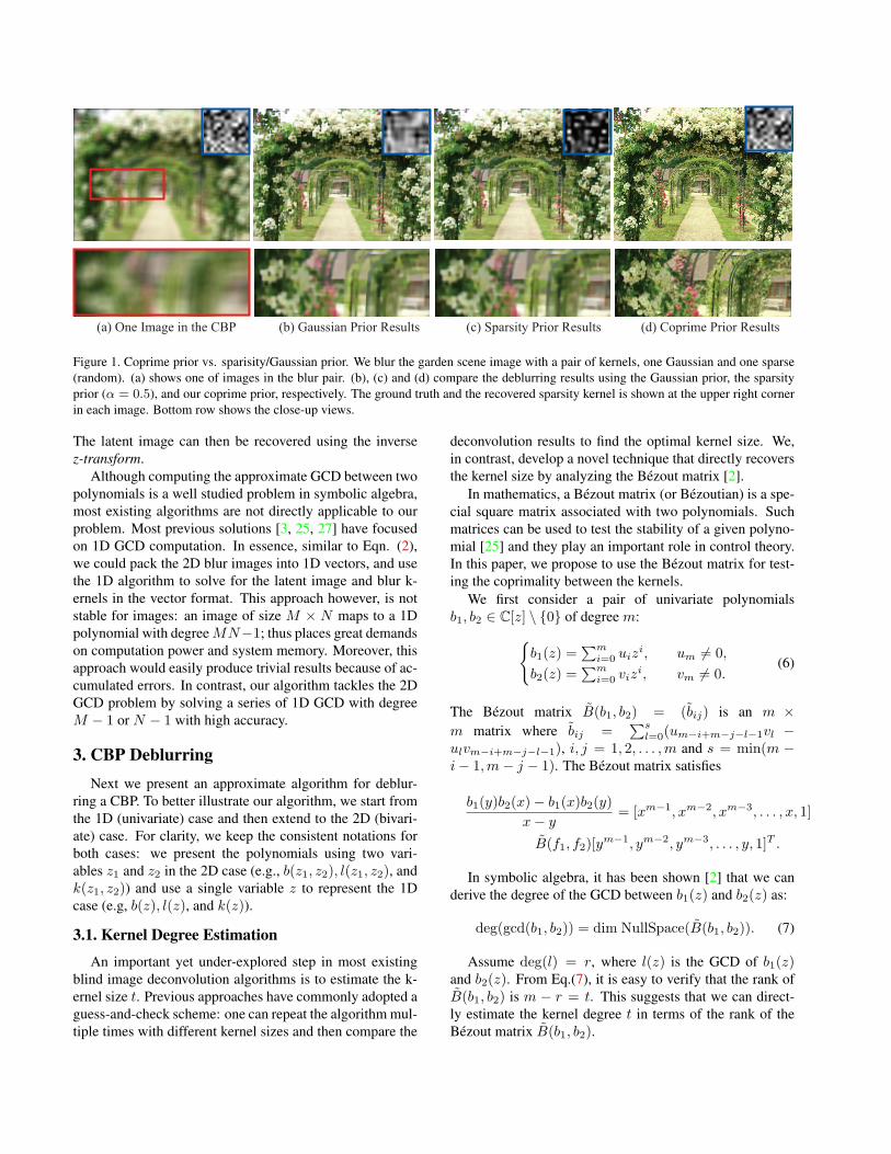
Figure 2. The processing pipeline of our CBP-based privacy-protected video surveillance.

it takes O(n2 log(n)) operations for FFT division. Hence,the overall complexity of our algorithm is O(n2 log(n)) forrecovering both the latent image and blur kernels in a CBPof image resolution n × n. Table. 1 shows the processingspeed of our CBP-based deblurring algorithm at differentimage and kernel resolutions.

4. CBP for SurveillanceAlthough image blurs have been commonly considered

adverse in computer vision, they also provide a naturalway for protecting the image contents and therefore can beused for information hiding. For example, concern aboutthe potential for abuse and the general loss of privacy invideo surveillance has also grown along with the numberof surveillance cameras. Maintaining security in sensitiveenvironments without impinging on the privacy of the pub-lic is a difficult balance to strike. Recently, the notion of”blind vision” has been introduced for addressing such pri-vacy issues. Recent efforts include privacy-protected facedetection [1], face recognition [8], image filtering [11], im-age retrieval [23], and video surveillance [26, 6, 5]. In lightof these recent efforts, we present a scheme based on CBPto achieve multi-level identity protection.

We develop a privacy-preserving surveillance scheme byapplying coprime blurs to the regular surveillance video da-ta to form a public stream and a private stream. By havingtheir contents blurred, the streams retain the ability to re-construct an unblurred image if and only if one has accessto both video streams simultaneously. Further, by carefullychoosing the blur kernels, the two streams will have differ-

Single Image

Deconvolution [Shan et al.]

Coprime Prior Result

Dual-Image Deblurring

with Sparsity Prior

One CBP

Encrypted Sequence

Frame 236 Frame 259 Frame 284 Frame 316

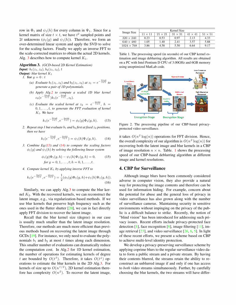
Figure 3. Decrypted results on video frames encrypted by our CBP scheme using different methods. Video data: courtesy of the EC FundedCAVIAR project/IST 2001 37540.

ent degrees of blurring in order to provide users with lowerclearance less access to personally identifiable details whilestill allowing behavior to be monitored.

Fig. 2 illustrates our CBP surveillance pipeline. We s-trategically perform two blurring operations by convolvingeach frame with two coprime kernels. At this state bothimage streams are suitable for distribution to users accord-ing to their clearance level. In the final stage an unblurredversion of the public video stream will be recovered by per-forming our CBP-based deblurring algorithm.

Our public/private image terminology is reminiscent ofRSA public key cryptography scheme [18]. It utilizes anasymmetrical key scheme that depends on a public key forencryption and a private key for decryption. Even thoughthe system provides all users with the recipient’s public keyonce the sender has encrypted the message with the pub-lic key it can only be decrypted with the recipient’s privatekey. Our approach applies the same principle by using alarge prime polynomial to blur private details within an im-age. Since it is very difficult to conduct blind image decon-

volution on a single stream [16] and all but users with thehighest clearance have access to only one polynomial kerneleach image stream by itself acts as a public key.

Just as the security of the RSA algorithm depends onkeeping the original two large prime numbers a secret oursystem relies on the two image streams being separate fromone another. The advantage of our approach is that by de-fault an individual image stream respects the privacy of thepublic and the second stream effectively acts as an addition-al layer of privacy and as a private key. Therefore as longas an eavesdropper does not have access to both streams theunblurred image cannot be recovered. Moreover, since ourCBP model provides a ´ partial` data encryption by strategi-cally blurring the image, low-clearance participants can stillanalyze the image contents (behavior, motion, etc.), whilethe data received by low-clearance participants would becompletely encrypted and visually useless when using theRSA algorithm.

In Fig. 3, we use two randomly generated blur kernel-s of size 21 × 21 to encrypt a surveillance video sequence

of resolution 384 × 288. We compare the deblurring re-sults obtained by our coprime dual-deblur algorithm (row4) and single image blind deconvolution [22] (row 2). Thevideo sequence captures a person walking towards the cam-era. Results produced by single-image deblurring containsstrong ringing artifacts that degrade the video quality. Byusing two blurred streams, our method is able to producevery high quality results, e.g., it accurately reconstructs theface of the subject.

5. DiscussionsLimitations of Sparsity Prior. Often, a pair of coprime

kernels are both coprime and sparse. This indicates that wecan also use the sparsity prior for recovering the kernels.We therefore further compare our CBP technique with thesparsity prior based solution. To effectively model sparsityof the kernel, we adopt a technique similar to the recent-ly proposed hyper-Laplacian scheme [15]. We use the ℓ0.5norm for the objective function (Eqn. 2) to emulate the s-parsity prior. We then apply the Iterative Re-weighted LeastSquares (IRLS) method [24, 15] to find the optimal solution.

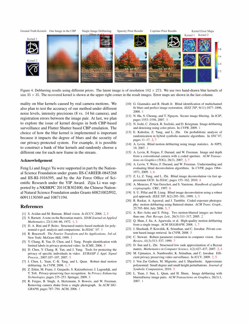
Fig. 3 (row 3) shows the recovered video sequence fromthe sparsity prior using the same dual-blur video pair. Com-pared with single-image blind deconvolution, the sparsityprior solution is able to greatly suppress the ringing artifact-s and produce reasonable results. However, it loses manyhigh frequency details compared to the CBP deblurring re-sults. Similar artifacts can be observed in Fig.4, wherewe blur the campus scene image using a pair of 35 × 35hand-drawn kernels. In our experiments, we found thatthe kernels produced by the sparsity prior tends to slight-ly ´ shrink` the kernels since it forces the kernels to be s-parse. This explains the loss of high frequency features inthe recovered latent image. Our method is able to preservedetails but exhibits some ringing artifacts. This is due tothe fact that the two hand-drawn kernels are not completelycoprime and our kernel estimation contains errors.

Flutter Shutter Implementation. To implement theCBP, the simplest way is to use a process post capture toimplement the blur. But with such methods there is somestage after capture where the image stream is not blurredand therefore susceptible to eavesdropping. To address thisissue, we suggest an on-capture solution, e.g., by using thefluttered shutter (FS) camera.

The FS camera developed by Raskar et al. [20] opensand closes the shutter during the exposure process accord-ing to a pre-determined sequence. The pseudo-random se-quence creates a broad-band filter that preserves high fre-quency details and is suitable for deconvolution. In the orig-inal FS work, the shutter sequence is assumed to be known[20]. We instead suggest using a pair of unknown but co-prime shutter sequences. For example, these coprime shut-ter sequences can be implemented by randomly generating

(a) (b)

(c) (d)

Open

Close

Shutter1

Time

Open

Close

Shutter2

Time

Figure 5. Constructing a CBP using a Flutter Shutter. (a) and (b)emulate two captured images of a moving object under two ran-domly chosen flutter shutter sequences. (c) shows our recoveredblur kernels. (d) shows our recovered latent image.

two shutter sequences since two random polynomials aregenerally coprime [13].

Unlike the original FS camera that assumes static cam-era and fast moving targets, we assume that the targets aremoving slowly and we emulate motion blurs on the camer-a side: we can mount the camera on an oscillating motorto introduce motion blurs during capture. Notice that thepath of oscillation does not need to be known but rather thatthe flutter sequence be prime to each other. There are manycomputer controlled motor systems that can reliably repro-duce small controlled oscillations at common frame rates.

In Fig. 5, we emulate our proposed FS implementationof CBP. We pick two random sequences (the top row ofFig. 5) and synthesize a pair of blurred images under 2Dmotions. We then directly apply our CBP deblurring tech-nique to obtain the blur-free images. Fig.5(d) shows ourdeblurred results. Since the FS sequences well preserveshigh frequencies and they are highly coprime (due to ran-dom sequence selection), we are able to accurately estimatethe two blur kernels and robustly deblur the images. We en-vision that the FS camera can be directly used to produceCBPs in the future. For example, we can mount a pair ofFS cameras on an oscillating motor to introduce artificialmotion blurs during capture. This will produce CBP videostreams that are suitable for privacy protection.

Limitations and Future Work. We have proposed anovel CBP theory that has the potential to benefit a num-ber of vision applications. We have by far focused on thetheoretical foundation of the CBP model and have only ap-plied our theory to privacy-protected video surveillance. Asimportant part of future work, we plan to capture real dualmotion-blurred image pairs [7] and test the validity of copri-

One Image in the CBP Single Image Deblurring

[Shan et al.]

Sparsity Prior Results Coprime Prior Results Kernel Error MapsGround Truth Kernels

Kernel 2

Kernel 1

Kernel 1 Kernel 2

Figure 4. Deblurring results using different priors. The latent image is of resolution 182 × 273. We use two hand-drawn blur kernels ofsize 35× 35. The recovered kernel is shown at the upper right corner in the result images. Error maps are shown in the last column.

mality on blur kernels caused by real camera motions. Wealso plan to test the accuracy of our method under differentnoise levels, intensity precisions (8 vs. 14 bit camera), andregistration errors between the image pair. At last, we planto explore the issue of kernel designs in both CBP-basedsurveillance and Flutter Shutter based CBP emulation. Thechoice of how the blur kernel is implemented is importantbecause it impacts the degree of blurs and the security ofour privacy-protected system. For example, it is possibleto construct a bank of blur kernels and randomly choose adifferent one for each new frame in the stream.

Acknowledgement

Feng Li and Jingyi Yu were supported in part by the Nation-al Science Foundation under grants IIS-CAREER-0845268and IIS-RI-1016395, and by the Air Force Office of Sci-entific Research under the YIP Award. Zijia Li was sup-ported by a NKBRPC 2011CB302400, the Chinese Nation-al Natural Science Foundation under Grants 60821002/F02,60911130369 and 10871194.

References[1] S. Avidan and M. Butman. Blind vision. In ECCV, 2006. 2, 5[2] S. Barnett. A note on the Bezoutian matrix. SIAM Journal on Applied

Mathematics, 22(1):84–86, 1972. 1, 3[3] D. A. Bini and P. Boito. Structured matrix-based methods for poly-

nomial e-gcd: analysis and comparisons. In ISSAC ’07. 3[4] R. Bracewell. The Fourier Transform and Its Applications, 3rd ed.

New York: McGraw-Hill, 1999. 1[5] Y. Chang, R. Yan, D. Chen, and J. Yang. People identification with

limited labels in privacy-protected video. In ICME, 2006. 5[6] D. Chen, Y. Chang, R. Yan, and J. Yang. Tools for protecting the

privacy of specific individuals in video. EURASIP J. Appl. SignalProcess., 2007:107–107, 2007. 5

[7] J. Chen, L. Yuan, C.-K. Tang, and L. Quan. Robust dual motiondeblurring. In CVPR, 2008. 1, 7

[8] Z. Erkin, M. Franz, J. Guajardo, S. Katzenbeisser, I. Lagendijk, andT. Toft. Privacy-preserving face recognition. In Privacy EnhancingTechnologies, pages 235–253. Springer, 2009. 5

[9] R. Fergus, B. Singh, A. Hertzmann, S. Roweis, and W. Freeman.Removing camera shake from a single photograph. In ACM SIG-GRAPH, pages 787–794. ACM, 2006. 1

[10] G. Giannakis and R. Heath Jr. Blind identification of multichannelfir blurs and perfect image restoration. IEEE TIP, 9(11):1877–1896,2000. 1

[11] N. Hu, S. Cheung, and T. Nguyen. Secure image filtering. In ICIP,pages 1553–1556, 2007. 5

[12] N. Joshi, C. Zitnick, R. Szeliski, and D. Kriegman. Image deblurringand denoising using color priors. In CVPR, 2009. 1

[13] E. Kaltofen, Z. Yang, and L. Zhi. On probabilistic analysis ofrandomization in hybrid symbolic-numeric algorithms. In SNC’07,pages 11–17. 2, 7

[14] A. Levin. Blind motion deblurring using image statistics. In NIPS,19, 2007. 1

[15] A. Levin, R. Fergus, F. Durand, and W. Freeman. Image and depthfrom a conventional camera with a coded aperture. ACM Transac-tions on Graphics (TOG), 26(3), 2007. 2, 7

[16] A. Levin, Y. Weiss, F. Durand, and W. Freeman. Understanding andevaluating blind deconvolution algorithms. In CVPR, pages 1964–1971, 2009. 1, 6

[17] Z. Li, Z. Yang, and L. Zhi. Blind image deconvolution via fast ap-proximate GCD. In ISSAC, pages 155–162, 2010. 4

[18] A. Menezes, P. Van Oorschot, and S. Vanstone. Handbook of appliedcryptography. CRC, 1997. 6

[19] S. U. Pillai and B. Liang. Blind image deconvolution using a robustgcd approach. IEEE TIP, 8(2):295–301, 1999. 1, 5

[20] R. Raskar, A. Agrawal, and J. Tumblin. Coded exposure photogra-phy: motion deblurring using fluttered shutter. ACM Trans. Graph.,25:795–804, July 2006. 5, 7

[21] A. Rav-Acha and S. Peleg. Two motion-blurred images are betterthan one. Patt. Recogn. Lett., 26(3):311–317, 2005. 2

[22] Q. Shan, J. Jia, A. Agarwala, et al. High-quality motion deblurringfrom a single image. ACM SIGGRAPH, 2008. 1, 7

[23] J. Shashank, P. Kowshik, K. Srinathan, and C. Jawahar. Private con-tent based image retrieval. In CVPR, 2008. 5

[24] C. Stewart. Robust parameter estimation in computer vision. SiamReview, 41(3):513–537, 1999. 7

[25] D. Sun and L. Zhi. Structured low rank approximation of a Bezoutmatrix. Mathematics in Computer Science, 1(2):427–437, 2007. 3, 4

[26] M. Upmanyu, A. Namboodiri, K. Srinathan, and C. Jawahar. Effi-cient privacy preserving video surveillance. In ICCV, 2009. 2, 5

[27] J. Von Zur Gathen, M. Mignotte, and I. Shparlinski. Approximatepolynomial: Small degree and small height perturbations. Journal ofSymbolic Computation, 2010. 3

[28] L. Yuan, J. Sun, L. Quan, and H. Shum. Image deblurring withblurred/noisy image pairs. ACM Transactions on Graphics, 26(3):1,2007. 1