Embed Size (px)
Citation preview

A Theoretical Foundation ofNetwork Localization andNavigationThis paper provides a theoretical foundation for the design of localization and navigationnetworks, paving the way to a new level of performance via spatiotemporal cooperation.
BY MOE Z. WIN , Fellow IEEE, YUAN SHEN , Member IEEE,AND WENHAN DAI , Student Member IEEE
ABSTRACT | Network localization and navigation (NLN) is a
promising paradigm, in which mobile nodes exploit spatiotem-
poral cooperation, to provide reliable location information for
a diverse range of wireless applications. This paper presents
a theoretical foundation of NLN, including a mathematical for-
mulation for NLN, an introduction of equivalent Fisher informa-
tion analysis, and determination of the fundamental limits of
localization accuracy. Key ingredients such as spatiotemporal
cooperation, array signal processing, and map exploitation are
then studied. We also develop a geometric interpretation to
provide insights into the essence of NLN for network design.
Finally, the paper highlights the connection between the theo-
retical foundation and algorithm development for NLN, guiding
the design and operation of practical localization systems.
KEYWORDS | Equivalent Fisher information; localization; navi-
gation; spatiotemporal cooperation; wireless network
I. I N T R O D U C T I O N
Location awareness is essential for a wide variety ofmodern civil and military applications [1]–[9], such
Manuscript received September 7, 2017; accepted April 9, 2018. Date of currentversion July 25, 2018. This work was supported in part by the U.S. Office of NavalResearch under Grant N00014-16-1-2141; and in part by the MIT Institute forSoldier Nanotechnologies. (Corresponding author: Moe Z. Win.)
M. Z. Win is with the Laboratory for Information and Decision Systems,Massachusetts Institute of Technology, Cambridge MA 02139 USA (e-mail:[email protected]).
Y. Shen was with the Wireless Information and Network Sciences Laboratory,Massachusetts Institute of Technology, Cambridge, MA 02139 USA. He is nowwith the Department of Electronic Engineering, Tsinghua University, and BeijingNational Research Center for Information Science and Technology, Beijing100084, China (e-mail: [email protected]).
W. Dai is with the Wireless Information and Network Sciences Laboratory,Massachusetts Institute of Technology, Cambridge MA 02139 USA (e-mail:[email protected]).
Digital Object Identifier 10.1109/JPROC.2018.2844553
as location-based services [10]–[12], rescue operations[13]–[15], autonomous vehicles [16]–[18], Internet-of-Things [19]–[21], health monitoring [22]–[24], andcrowdsensing [25]–[27]. In outdoor environments,numerous location-based applications benefit from themeter-level positioning capability of the prominentglobal navigation satellite system (GNSS) technology[29]–[35]. Unfortunately, due to the weak signalsfrom the satellites, such positioning capability becomesunreliable or even completely inaccessible in harshpropagation environments (e.g., in buildings, urbancanyons, and underground) [1]–[4]. Moreover, emergingapplications such as autonomous vehicles may requirea higher positioning accuracy than the current GNSStechnology. To address the urgent need for high-accuracylocation awareness, there have been tremendous researchinterests and efforts from both academia and industry inrecent years [36]–[53].
Localizing mobile nodes with unknown positions (calledagents) can be accomplished by utilizing two types ofmeasurements, namely, inter-node and intra-node mea-surements, together with prior knowledge [54]–[58] Inter-node measurements refer to those between nodes ina network through radio-frequency (RF) transmission[59]–[63], vision sensing [64]–[66], Lidar [67]–[69],and ultrasound [70]–[72]. Typical examples of RF trans-mission include the relative distance, angle, or vicinitybetween two nodes measured by Wi-Fi, RF identifica-tion (RFID), ultrawideband (UWB), and frequency mod-ulation (FM) radios. With the aid of a few nodes thathave perfectly known positions (called anchors), inter-node measurements to these anchors can be used toestimate the agent position through multilateration ortriangulation [73]–[75]. Comparatively, intra-node mea-
1136 PROCEEDINGS OF THE IEEE | Vol. 106, No. 7, July 2018
0018-9219 © 2018 IEEE. Personal use is permitted, but republication/redistribution requires IEEE permission.See http://www.ieee.org/publications_standards/publications/rights/index.html for more information.

Win et al.: A Theoretical Foundation of Network Localization and Navigation
surements refer to those with respect to an agent itself,which do not involve interaction with other nodes. Typicalexamples include angular velocities and accelerations ofa node obtained by inertial measurement units (IMUs)[76]–[81], or feature points in images captured by visionsensors [82]–[85]. Inertial measurements can be used toreconstruct the agent’s trajectory, while the feature pointsin multiple images can be used to estimate the agentmovement [81]–[83]. In addition, prior knowledge aboutthe agent positions is another source of information thatbenefits localization systems. For example, harnessing mapinformation can effectively improve the localization perfor-mance in both theory and practice [86]–[90].
Commonly used signal metrics for RF-based rangemeasurements include time-of-arrival (TOA) [91]–[97],timedifference- of-arrival (TDOA) [98]–[100], andreceived signal strength (RSS) [101]–[104].1 Time-based metrics, such as TOA and TDOA, are obtainedby measuring the signal propagation time betweennodes, and RSS can be obtained by a low-cost energyaccumulator. These metrics can be used to estimateinter-node distances together with the propagation speedor the channel fading model. Commonly used signalmetrics for RF-based angle measurements include thedirection-of-arrival (DOA) and the angle-of-arrival (AOA)[109]–[118]. Such metrics can be obtained by the carrier-phase difference of the signals received at an array ofantennas, or directly using angular antennas [119]–[121].With sufficient transmission power, signal bandwidth, orarray aperture, these techniques can potentially achievesubmeter localization accuracy [4]–[6].
The aforementioned GNSS can be considered as anRF-based localization technology, which estimates the posi-tion of a mobile user based on the TDOAs of the signalstransmitted from several satellites [28]–[30]. In GNSS-challenged environments, terrestrial wireless networks areemployed as a principal complement for providing posi-tioning capability [1]–[4], where each agent is usuallylocalized using the range and angle measurements to thebase stations with known positions.
In contrast to conventional localization techniques, thenetwork localization and navigation (NLN) paradigm pro-posed in [1] advocates that agents jointly infer theirstates (e.g., position, velocity, acceleration, etc.) by coop-erative techniques in both spatial and temporal domains(see Fig. 1 for the general concept). In the spatialdomain, each agent obtains information about its staterelative to other nodes’ states by inter-node measurements(e.g., ranges). Spatial cooperation between agents involvesexploiting the internode measurements of agent-agentpairs in addition to those of agent-anchor pairs, as wellas sharing location information between agents for local-ization. Such cooperation has been shown to remarkably
1As a side note, RSS can also be used as a fingerprint to matchthe entries in the database for localization with the aid of training[105]–[108]. However, the fingerprint-based techniques require extensivetraining for satisfactory localization performance.
Fig. 1. An example of NLN: a network with three agents (blue
circles) moving along the dashed trajectories. The empty ones
denote those at time instant t� and the solid ones at time instant t�.
Intra-node measurements and inter-node measurements are
denoted by green and red arrows, respectively.
improve the localization performance, especially when theanchors cannot provide highquality measurements to theagents [54]–[58], [122]–[126]. To unleash the potentialof spatial cooperation, there is a rich literature on thetheory and algorithms in recent years [127]–[136]. In thetemporal domain, each agent obtains information about itsstate relative to those in previous instants by intra-nodemeasurements (e.g., accelerations). Those measurementsprovide the information about the state evolution overdifferent instants and can significantly benefit localizationthrough a filtering process [77]–[81].
Joint spatial and temporal cooperation of NLN canyield dramatic localization performance improvement overconventional approaches since additional information isexploited through cooperation with other nodes and otherinstants [54]–[56]. In particular, measurements amongagents through cooperation contribute to the entire net-work from the inference point of view. However, joint spa-tial and temporal cooperation incurs associated costs suchas additional communication and more complicated algo-rithms over the network: 1) the communication amongnodes is required for inter-node measurements and infor-mation exchange; and 2) interdependency among theestimates of the agent positions hinders effective distrib-uted inference algorithms [137]–[139]. Thus, to provideperformance benchmarks and to guide efficient networkdesign and operation, it is important to understand thefundamental limits of localization accuracy in NLN as wellas the corresponding approaches to achieve such accuracy.2
For this purpose, the information inequality can be appliedto determine a lower bound for the estimation errors,which is known as the Cramér-Rao lower bound (CRLB),through the inverse of the Fisher information matrix (FIM)[140]–[143]. The CRLB is desirable for analysis in various
2For example, in designing energy-efficient localization networks,attainable localization accuracy is a meaningful performance objective.
Vol. 106, No. 7, July 2018 | PROCEEDINGS OF THE IEEE 1137

Win et al.: A Theoretical Foundation of Network Localization and Navigation
applications due to its amenable properties and asymp-totical achievability in high signal-to-noise ratio (SNR)regimes. In low SNR regimes, other bounds such as the Ziv-Zakai bound (ZZB) and Weiss-Weistein bound (WWB) aremore suitable than the CRLB but with highly complicatedexpressions [144]–[149].
To evaluate the localization performance in the pres-ence of noise, CRLB-type performance bounds for certainsignal metrics, e.g., time delays or AOAs, are obtainedin [150]–[155]. Note that the property of the signalmetrics depends heavily on the signal processing proce-dures, and the use of certain signal metrics may discardrelevant information for localization. Thus, in derivingthe fundamental limits of localization accuracy, it is nec-essary to fully exploit the information contained in thereceived waveforms rather than using specific signal met-rics extracted from the waveforms [156]–[158]. Based onthe received wideband signals, the fundamental limits oflocalization accuracy for a single agent are derived in [5],and the results have been generalized to the multiple-agent scenario with spatial cooperation in [54]. In additionto spatial cooperation, temporal cooperation via intra-node measurements is incorporated in the analysis forthe dynamic scenarios, where the information evolution ischaracterized in both spatial and temporal domains [55].Moreover, recent studies show that the TOA and AOAinformation obtained from modulated signals by antennaarrays can be characterized in a unified way, where thebaseband signal and the carrier signal play the role in therange and angular measurements, respectively [159].
The position inference in NLN can benefit fromthe availability of prior knowledge. Among others, themap information has been exploited in localizationalgorithms, which effectively improves the localizationaccuracy [86]–[88]. For map information modeled as aprior distribution, bounds such as the ZZB and WWB aremore suitable than the CRLB to capture the informationprovided by the map. To this end, the impact of mapinformation for localization is studied using the ZZB andWWB in [89] and [90]. The corresponding performancebounds are tighter than the CRLB in the median tolow SNR regimes. These bounds give new insights intothe use of map information for localization and howone should exploit such information in the localizationalgorithm.
This paper provides a theoretical foundation for NLN inwhich nodes exploit joint spatial and temporal cooperationfor position inference. We determine the performance lim-its of a localization network employing spatial cooperationvia inter-node wireless measurements, temporal coopera-tion via intra-node IMU measurements, as well as the priorposition knowledge via map information. The main bodyof the paper consists of five components as follows.
• We present a general mathematical model for NLNthat exploits all the position-related information (e.g.,distance and angle) from the inter-node and intran-ode measurements in a unified way.
• We develop the equivalent Fisher information (EFI)analysis to determine the fundamental limits of NLNand show that the location information can be decom-posed into basic building blocks, each associated witha spatial or temporal measurement.
• We develop a geometric interpretation for the locationinformation using the notion of information ellipse,by which the spatiotemporal evolution of the locationinformation is characterized.
• We quantify the use of map information as priorknowledge for localization by the ZZB and WWB,revealing the region of SNR where the map informa-tion plays a critical role.
• We show how the theoretical foundation canguide the system design via numerical examples,through which the effects of system parameters,spatiotemporal cooperation, and the map informationare quantified.
The remaining sections are organized as follows.Section II presents the system model for NLN and themethodology for EFI analysis. Section III derives thefundamental limits for noncooperative localization net-works, and Section IV extends the analysis to spatiotem-poral cooperative cases. Section V presents the notionof information ellipse to illustrate the behavior of thelocation information. Section VI discusses the use ofmap information in localization and introduces typicallocalization algorithms. Section VII presents the guide-lines obtained from the theoretical foundation to networkdesign by numerical examples. The last section draws theconclusions.
Notations: Throughout this paper, variables, vectors,and matrices are written as italic letters x, bold italicletters x, and bold capital italic letters X , respectively.Random variables, random vectors, and random matricesare written as sans serif letter x, bold letters x, and boldcapital letters X, respectively. The 0m and 1m denotevectors of length m with all 0’s and 1’s, respectively;[A]ij is an element at the ith row and jth column ofmatrix A. The notation A � B denotes that the matrixA−B is positive semi-definite; tr{A},AT, |A|, and adj(A)
denote the trace, transpose, determinant, and adjugatematrix of A, respectively; ‖x‖ denotes the Euclidean normof x; and S
n++ and S
n+ denote the set of n × n positive-
definite and positive-semidefinite matrices, respectively.Define the unit vectors u(ϕ) := [ cosϕ sinϕ ]T. Thenotation xk1:k2 is used for concatenating the set of vectors{xk1 ,xk1+1, . . . ,xk2}, for {x(t1),x(t1+1), . . . ,x(t2)}, andx
(t1:t2)k1:k2
for {x(t1)k1:k2
,x(t1+1)k1:k2
, . . . ,x(t2)k1:k2
} for k1 � k2, t1 �t2. The notation N (μ,Σ) denotes a Gaussian distributionwith mean μ and covariance matrix Σ. We denote ⊗ theKronecker product andEN
i,j theN×N matrix with all zerosexcept a 1 on the ith row and jth column.
The functions fx(x), fx(x; θ), fx|y(x|y) denote the prob-ability density function (PDF) of x, the PDF of x para-meterized by θ, and the conditional PDF of x given y,
1138 PROCEEDINGS OF THE IEEE | Vol. 106, No. 7, July 2018

Win et al.: A Theoretical Foundation of Network Localization and Navigation
respectively. We also define the functions
jbm(z, a(θ1, θ2, θ3), θ1, θ2) : =∂ ln fz(z; a(θ1, θ2, θ3))
∂θ1
·∂ ln fz(z; a(θ1, θ2, θ3))
∂θT2
jbp(b(θ1, θ2), θ3, θ1, θ2): =∂ lnfb(θ1,θ2)|θ3(b(θ1, θ2)|θ3)
∂θ1
·∂ lnfb(θ1,θ2)|θ3(b(θ1,θ2)|θ3)
∂θT2
.
The notation Ex{·} is the expectation operator with respectto the random vector x. The subscripts of f and E may beomitted for brevity when clear from the context.
II. S Y S T E M M O D E L
This section first presents the network setting, the statemodel, and the measurement models for NLN, and thenreviews the notion of the information inequality and thetechnique of the EFI analysis.
A. Network Setting
Consider a wireless network consisting of Na agents andNb anchors. The sets of agents and anchors are denoted byNa = {1, 2, . . . , Na} and Nb = {Na+1, Na+2, . . . , Na+Nb},respectively. Both the measurements and inference areperformed at discrete time instants tn’s (n = 1, 2, . . . , N).The state of node k at time tn is denoted by vector x(n)
k ,which can include the agent position, velocity, accelera-tion, orientation, and angular velocity.
The goal of NLN is to determine the states of agentsfrom inter-node and intra-node measurements as well asmap information, whenever available. We denote the setof measurements made at time tn by z(n), which is theconcatenation of vectors z(n)
kj , k ∈ Na, j ∈ Na ∪ Nb. Thenotations z(n)
kj for k �= j represent inter-node measure-ments, while z(n)
kk represent the intra-node measurementsof agent k.
The parameter vector of the NLN problem includesthe agent states and nuisance parameters associated withinternode and intra-node measurements. We denote theparameter vector at time tn by
θ(n) =�x
(n) T1:Na
κ(n) T1:Na
�T(1)
where the measurement parameter vector κ(n)k is formed
by the concatenation of vectors κ(n)kj , j ∈ Na∪Nb, in which
κ(n)kj (k �= j) is associated with the inter-node measure-
ments from node k to node j, and κ(n)kk is associated with
the intra-node measurements of node k.Note that although these measurement parameters such
as clock drifts and channel amplitudes are not of interestfor the NLN problem, they need to be considered sincetheir estimation errors affect the performance of positioninference. For example, the unknown clock drift will lead
to degraded intra-node velocity estimation or inter-nodeTOA estimation.
B. State Models
This section describes the models for the states fromthe non-Bayesian and Bayesian perspectives, i.e., modelingthe states as deterministic unknown parameters or randomparameters, respectively.
1) Non-Bayesian Model: The agent states and nuisanceparameters associated with the measurements are mod-eled as deterministic unknown parameters, i.e., their priorknowledge is not available. The state x(n)
k consists of theposition and orientation of the agent k at time tn, andthe measurements z(n) at time tn depend on the agentpositions and orientations at consecutive instants.3
Let θ = θ(1:N) and z = z(1:N). The likelihood function ofthe measurements can be written as
f(z; θ) =N�
n=1
f�z(n);x(n−n0:n),κ(n)� (2)
where x(n) consists of agent positions p(n)k and orienta-
tions ω(n)k , and the choice of n0 depends on the type
of measurements. For example, n0 is set to 2 whenthe intra-node measurements z(n) is related to agentaccelerations.
Given the agent states and nuisance parameters, themeasurements made by different sensors are assumed tobe independent. Therefore, the measurement model in (2)can be decomposed into inter-node and intra-node mea-surements as
f(z; θ) =N�
n=1
�k∈Na
�f�z
(n)kk ;x
(n−n0:n)k ,κ
(n)kk
�� � intra−node measurements
·�
j∈Na∪Nb\{k}f�z
(n)kj ;x
(n−n0:n)k ,x
(n−n0:n)j ,κ
(n)kj
�� � inter−node measurements
�.(3)
2) Bayesian Model: In contrast to the non-Bayesianmodel, the agent states and nuisance parameters asso-ciated with the measurements are modeled as randomvariables. The dynamics of these random variables and themeasurements are usually described by a hidden Markovmodel (HMM) [160]–[162], and the pdf of the measure-ments z and parameters θ is then
f(z, θ) =N�
n=1
f�θ(n)|θ(n−1)�� �
dynamic model
f�z(n)|θ(n)�� �
measurement model
(4)
3For example, acceleration and angular velocity measurements canbe represented by the positions and orientations of the agents atconsecutive instants, as will be shown in Section II-C.
Vol. 106, No. 7, July 2018 | PROCEEDINGS OF THE IEEE 1139

Win et al.: A Theoretical Foundation of Network Localization and Navigation
where θ(0) := ∅ is the empty set for notational conve-nience.
Similar to the non-Bayesian model, given the agentstates and nuisance parameters, the measurements madeby different sensors are assumed to be independent,and thus the measurement model can be furtherdecomposed as
f�z(n)|θ(n)
�=
�k∈Na
�f�z
(n)kk
��x(n)k ,κ
(n)kk
�� � intra−node measurements
·�
j∈Na∪Nb\{k}f�z
(n)kj
��x(n)k ,x
(n)j ,κ
(n)kj
�� � inter−node measurements
�(5)
where x(n)k may include the agent positions, velocities,
accelerations, orientations, and angular velocities, depend-ing on the type of measurements.
Remark 1: In the non-Bayesian model, no prior knowl-edge about the dynamic evolution of the states is assumed,whereas in the Bayesian model, the dynamics of the statesare modeled by an HMM via f(θ(n)|θ(n−1)). Moreover, inthe non-Bayesian model (3), the states consist of only thenode positions and orientations, and the measurementsfor quantities such as velocities and accelerations can bemodeled by a function of the states at consecutive instants,whereas in the Bayesian model (4), the states directlyinclude all the fundamental physical quantities related todynamics.
While we focus on the non-Bayesian models in thispaper, most results are applicable to the Bayesian mod-els with some modifications. For several key conclusions,remarks will be included for the Bayesian models.
C. Measurement Models
We next provide the mathematical models for generalinter-node and intra-node measurements based on thenon- Bayesian models of the states, i.e., the state onlyconsists of the positions and orientations.
1) Inter-node Measurements: The inter-node measure-ments, denoted by z(n)
kj , are performed by node k withrespect to node j. Examples of such measurements includethose obtained from the RF or acoustic signals transmittedfrom node j and received by node k, or the image of nodej captured by node k’s vision sensor. In general, inter-nodemeasurements depend only on the difference between thestates of the two nodes. We next detail the relative positionand velocity measurements.4
• Relative position: Node relative positions can be mea-sured by, for example, RF or acoustic signals. Thus, bychoosing n0 = 0, the measurement for node relative
4To the best of the authors’ knowledge, there are no sensors yetthat can directly measure the relative acceleration, relative orientation,or relative angular velocity.
positions can be described as
z(n)kj = g0
�p(n)
k − p(n)j ,κ
(n)kj
�+ w
(n)kj (6)
where g0(·) denotes a function of node relative posi-tions, and w(n)
kj represents the random measurementnoise. The likelihood of the position measurementin (3) can then be written as
f�z
(n)kj ;x
(n)k ,x
(n)j ,κ
(n)kj
�=f
w(n)kj
�z
(n)kj −g0
�p(n)
k −p(n)j ,κ
(n)kj
�; p(n)
k ,p(n)j ,κ
(n)kj
�. (7)
• Relative velocity: Node relative velocities can be mea-sured by, for example, RF or acoustic signals via theDoppler shifts. Since the velocity can be modeledas the first-order difference of node positions, bychoosing n0 = 1, the measurement for node relativevelocities can be described as5
z(n)kj =g1
�p(n)
k −p(n−1)k −p(n)
j +p(n−1)j ,κ
(n)kj
�+w(n)
kj (8)
where g1(·) denotes a function of node relativevelocities. Then, the likelihood of the relativevelocity measurement can be written similarlyas (7).
2) Intra-node Measurements: The intra-node measure-ments, denoted by z
(n)kk , are performed by node k itself.
Examples of such measurements include those fromIMU and vision sensors. Note that the measurementsrelated to velocities and accelerations can be modeledas a function of the agent positions and orientationsat consecutive instants. Thus, the likelihood functionf(z
(n)kk ;x
(n−n0:n)k ,κ
(n)kk ) in (3) for different types of intra-
node measurements corresponds to different values of n0.We exemplify the likelihood function for several typicalmeasurements in the following.
• Position: Node positions can be measured directlyby, for example, a vision or Lidar sensor through aknown local reference. Thus, by choosing n0 = 0, themeasurement for node positions can be described as
z(n)kk = h0
�p(n)
k ,κ(n)kk
�+ w(n)
k (9)
where h0(·) denotes a function of node positions,and w(n)
k represents the random measurement noise.Then, the likelihood of the position measurement canbe written in a similar way as (7).
• Velocity: Node velocities are usually obtained byDoppler measurements and can be modeled as thefirst-order difference of node positions. Thus, by
5We reuse the notation w(n)kj as in (6) for the relative velocity mea-
surement noise, with the understanding that it corresponds to differentmeasurements.
1140 PROCEEDINGS OF THE IEEE | Vol. 106, No. 7, July 2018

Win et al.: A Theoretical Foundation of Network Localization and Navigation
choosing n0 = 1, the measurement for node velocitiescan be described as
z(n)kk = h1
�p(n)
k − p(n−1)k ,κ
(n)kk
�+ w
(n)k (10)
where h1(·) denotes a function of node velocities.• Acceleration: Node accelerations are usually
measured by an IMU and can be modeled asthe secondorder difference of node positions.6 Thus,by choosing n0 = 2, the measurement of nodeaccelerations can be described as
z(n)kk = h2
�p(n)
k − 2 p(n−1)k + p(n−2)
k ,κ(n)kk
�+ w(n)
k (11)
where h2(·) denotes a function of node accelerations.• Orientation: Analogous to node positions, node orien-
tations can be measured by a magnetometer, a visionsensor, or Lidar through a known local reference. Themeasurement for node orientations can be describedsimilarly as (9) with p(n)
k replaced by ω(n)k and corre-
sponding function h0(·).• Angular velocity: Analogous to node velocities, angu-
lar velocities are usually measured by a gyroscopeand can be modeled as the first-order difference ofnode orientations. The measurement for node angularvelocities can be described similarly as (10) with p(n)
k
replaced by ω(n)k and corresponding function h1(·).7
3) Special Case of Measurements: Sections II-C1 andII-C2 have described general forms of inter-node andintranode measurements. To provide more insights intoNLN, we next present the special case of the mea-surements that are used for developing the theoreticalfoundation.
We consider the inter-node measurements to beobtained by means of exchanging RF signals betweenthe nodes in quasi-static scenarios.8 The wireless signaltransmitted from node j and received by node k over asingle-path propagation channel can be written as
z(n)kj (t) = α
(n)kj s
�t− τ
(n)kj
�+ w
(n)kj (t), t ∈ [ 0, Tob) (12)
where s(t) is a known waveform (with Fourier transformdenoted by S(f)), α(n)
kj and τ(n)kj are the amplitude and
delay of the path, respectively, w(n)kj (t) represents the obser-
vation noise modeled as additive white Gaussian processeswith two-sided power spectral density N0/2, and [ 0, Tob)
6For simplicity, we consider accelerations measured in the globalcoordinates here, though the measurements by IMUs are in the localcoordinates.
7The relationship between the angular velocity and the orientationneed to be treated with care for 3-D cases [76].
8The signal metrics, such as TOA and AOA, can be used toestimate the relative position between the nodes. With the advance ofwideband transmission and array signal processing technologies, one canobtain accurate TOA and AOA measurements, which are essential forhighaccuracy localization.
is the observation interval. The relationship between τ (n)kj
and the node positions is
τ(n)kj =
1
c
�� p(n)k − p(n)
j
�� + b(n)kj
�(13)
where c is the propagation speed of the signal, and b(n)kj
denotes the range bias. The bias b(n)kj = 0 and b(n)
kj > 0 forline-of-sight (LOS) and non-line-of-sight (NLOS) propaga-tion, respectively [61].
Let z(n)kj be the vector representation of signal z
(n)kj (t)
obtained by the Karhunen-Loéve expansion [140], andthen the likelihood function of z(n)
kj , as a special case of (7),can be written as [5]
f(z(n)kj ; p(n)
k ,p(n)j ,κ
(n)kj )
∝ exp
�2
N0
� Tob
0
z(n)kj (t)α
(n)kj s
�t− τ
(n)kj
�dt
− 1
N0
� Tob
0
�α
(n)kj s
�t− τ
(n)kj
��2dt
�(14)
where the delay τ(n)kj is a function of p(n)
k and p(n)j as
described in (13), and the path amplitude α(n)kj and the
NLOS bias b(n)kj form the nuisance parameter vector κ(n)
kj .Finally, we consider the simplest but nontrivial case
for intra-node measurements, i.e., velocity measurementswith additive Gaussian noises given by
z(n)kk = p(n)
k − p(n−1)k + w
(n)k (15)
where w(n)k ∼ N (0, σ2
m I2) in which σm is a known con-stant.
D. Information Inequality and EFI Analysis
To evaluate the performance of NLN, we first brieflyreview the information inequality, which gives a lowerbound on the mean squared error (MSE) of estimators[140]. Consider a general measurement model f(z; θ) forthe observation z and unknown deterministic parametervector θ. Let T (z) be any estimator of some function ofθ, denoted as g(θ). Under some regularity conditions, thefollowing information inequality holds
E
�[T (z)−g(θ) ][T (z)−g(θ) ]T
�� ∂ψ(θ)
∂θJ−1
θ
∂ψ(θ)
∂θ
�T(16)
where ψ(θ) = E�T (z)
�and
Jθ = E�jbm(z, θ, θ, θ)
�(17)
is the FIM about θ. In particular, if g(θ) = θ and T (z) isan unbiased estimator, then ψ(θ) = θ and (16) reduces
Vol. 106, No. 7, July 2018 | PROCEEDINGS OF THE IEEE 1141

Win et al.: A Theoretical Foundation of Network Localization and Navigation
to [140]–[142]
E�[T (z) − θ ][T (z) − θ ]T
�� J−1
θ . (18)
In practice, only a small part of θ may be of interest.For example, let θ =
�θT
1 θT2
�T, where θ1 is a vectorof parameters of interest and θ2 is a vector of nuisanceparameters. Following (18), we have
E�[T 1(z) − θ1 ][T 1(z) − θ1 ]T
���J−1
θ
�θ1
(19)
where T 1(z) is an unbiased estimator of θ1 and [J−1θ ]θ1
denotes the square submatrix of J−1θ corresponding to θ1.
Evaluating J−1θ may be complicated since θ can be a
vector of high dimensions, while only a relatively smallsubmatrix [J−1
θ ]θ1is of interest. To obtain better insights,
we introduce the methodology of EFI analysis [5].
Definition 1 (EFIM): Given a parameter vectorθ = [ θT
1 θT2 ]T and the FIM Jθ of the form
Jθ =
�A B
BT C
�(20)
where θ ∈ RN , θ1 ∈ R
n, A ∈ Rn×n, B ∈ R
n×(N−n), andC ∈ R
(N−n)×(N−n) with 1 ≤ n < N , the equivalent Fisherinformation matrix (EFIM) for θ1 is given by
Je(θ1) := A −BC−1BT. (21)
Note that the EFIM Je(θ1) is the Schur complement ofthe block C in the original FIM Jθ [163], and it retainsall the necessary information to derive the informationinequality for θ1. In other words, the EFIM can be of amuch lower dimension than the original FIM without lossof information for the parameters of interest. In fact, onecan verify that the right-hand side of (19) is equal to theEFIM for θ1, i.e.,
[J−1θ ]θ1
= J−1e (θ1). (22)
Therefore, in the context of NLN and the systemmodel (2), by letting θ1 = x, we can obtain the EFIM forthe state x with the corresponding information inequalityas
E�(x − x)(x − x)T� � J−1
e (x). (23)
Moreover, the EFIM can be further applied to derive theinformation inequality for a certain subset of the states x,such as the position of an agent at a given instant. Thisleads to the following definition of the position errorbound.
Definition 2 (SPEB): The squared position error bound(SPEB) for the position of agent k at time tn is defined as
P( p(n)k ) := tr
��J−1
e (x)�
p(n)k
�(24)
where [J−1e (x)]
p(n)k
denotes the submatrix of J−1e (x) cor-
responding to p(n)k .
III. F U N D A M E N TA L L I M I T S O FL O C A L I Z AT I O N A C C U R A C Y
For ease of exposition, in this paper, we will mainly con-sider 2-D scenarios and assume that the inter-node mea-surements to be wireless signals modeled by (12) and theintra-node measurements only involve relative positions,i.e., n0 = 1 in (3).9
In the simplified scenarios, the states are the agentpositions denoted by x = p(1:N)
1:Na, and the inter-node and
intra-node measurements are the received wireless signalsz(n)kj (t) given by (12) and velocity measurements given
by (15), respectively. Thus, the parameter vector at timetn given in (1) can be written as
θ(n) =�
p(n) T1:Na
κ(n) T1:Na
�T(25)
where the nuisance parameters κ(n)kk = ∅, and κ
(n)kj =
[α(n)kj ∅ ]T and [α
(n)kj b
(n)kj ]T for LOS and NLOS signals,
respectively. In this section, we focus on the simplest casein which the agents in a static network do not cooperatewith each other.10 This case essentially translates to thescenario in which N = 1 and Na = 1. The set ofmeasurements only consists of those between agent 1 andthe anchors, i.e., {z1j}j∈Nb , and the parameters of interestare agent 1’s position p1, where the superscript is omittedfor brevity as we consider only one instant.
A. Synchronous Networks
We first derive the EFIM Je ( p1) for agent 1’s positionwhen the agent and the anchors are all synchronized. Thederivation is outlined in the following two steps. First,we show that the NLOS signals can be eliminated fromthe original FIM without loss of information for agent 1’sposition, resulting in an intermediate EFIM with a reduceddimension. Second, the channel parameters can be furthereliminated by applying the EFI analysis to obtain the EFIMfor agent 1’s position, i.e.,
Jθ = Je({ p1, {κ1j}j∈Nb})→ Je({p1, {κ1j}j∈Nb, LOS}) → Je( p1)
9The framework can be easily extended to multipath, dynamic, or3-D scenarios by augmenting the state and nuisance parameter vectorsto include additional parameters specific to each scenario.
10The cases of the spatiotemporal cooperation will be presented inthe next section.
1142 PROCEEDINGS OF THE IEEE | Vol. 106, No. 7, July 2018

Win et al.: A Theoretical Foundation of Network Localization and Navigation
Fig. 2. A network with four anchors and one agent. Anchor 5 does
not provide any RI due to NLOS propagation, while each other
anchor provides agent 1 with the RI of intensity λ�j along the
direction from the anchor to agent 1. The purple ellipse denotes the
information ellipse (described in Section V) obtained by agent 1.
where Nb, LOS and Nb, NLOS denote the sets of anchors thatprovide LOS and NLOS signals to agent 1, respectively.The final EFIM Je( p1) is of a much lower dimension thanthe original FIM but retains all the necessary informationfor p1.
Before stating the theorem, we introduce the notion ofrange information (RI) that constitutes the building blocksof the location information in two-dimensional networksas follows [5].
Definition 3 (Range Information): The RI is a 2 × 2
matrix of the form λJr(φ), where λ is a nonnegativenumber called the range information intensity (RII), andJr(φ) is a 2 × 2 matrix called the ranging direction matrix(RDM) with angle φ, given by
Jr(φ) :=
�cos2 φ cosφ sinφ
cosφ sinφ sin2 φ
�. (26)
Theorem 1 [5, Th. 1]: When the prior knowledge of thechannel and position parameters is not available, the EFIMfor agent 1’s position is given by
Je( p1) =�
j∈Nb, LOS
λ1j Jr(φ1j) (27)
where λ1j is the RII from anchor j, given by
λ1j =8π2β2
c2SNR1j (28)
and φ1j is the angle from agent 1 to anchor j. In (28), β isthe effective bandwidth and SNR1j is the SNR of the signal,given by
β :=
�� +∞−∞ f2 |S(f)|2df� +∞−∞ |S(f)|2df
�1/2
(29a)
SNR1j :=|α1j |2
� +∞−∞ |S(f)|2dfN0
. (29b)
Remark 2: The theorem and its extensions reveal impor-tant insights into the essence of network localization,showing how the NLOS condition, multipath propagation,signal bandwidth, and network geometry affect the local-ization accuracy (see Fig. 2).
• NLOS conditions: The NLOS signals do not contributeto the EFIM for the agent position, i.e., RII λ1j = 0
for j ∈ Nb, NLOS, when there is no prior knowledgeabout the NLOS biases. This is because the intern-ode distance obtained from the delay of the NLOSsignals are corrupted by the unknown biases b1j .Hence, the NLOS signals do not affect the informationinequality.11
• Multipath propagation: The EFIM (27) is also applica-ble to multipath propagation scenarios in which thereceived signal is modeled as
zkj(t) =
L�l=1
αkj,l s�t− τkj,l
�+wkj(t), t∈ [ 0, Tob)
(30)
where L is the number of multipath components(MPCs), and αkj,l and τkj,l are the amplitude anddelay of the lth path, respectively. In such scenarios,the RII (28) becomes [5]
λ1j =8π2β2
c2(1 − χ1j) SNR1j (31)
where χ1j ∈ [ 0, 1), referred to as the path-overlapping coefficient, characterizes the degradationof RII due to multipath propagation. With the sameSNR1j of the first path, the RII for the multipathcase (31) is smaller than that for the single-path case,given by (28). The degradation is caused by MPCsinterfering the estimation of the arrival time of thefirst path. The amount of degradation is determinedby the effective bandwidth of the signal s(t) and theinterpath delays of the MPCs in the first contiguouscluster of the received signal.12 As a special case whenthe first path is resolvable from the rest of the MPCs,there is no degradation and the RII reduces to that insingle-path scenarios.
• Bandwidth: The RII λ1j is proportional to theSNR and the squared effective bandwidth of thetransmitted signal s(t). That is, doubling the SNR can
11Nevertheless, NLOS signals can be useful in localization algo-rithms, e.g., resolving the ambiguity of agent positions or facilitatingthe search of agent positions.
12The first contiguous cluster [5, Def. 3], includes the MPCsthat cannot be completely resolved from the first path. The path-overlapping coefficient depends on the interpath delays of theMPCs in the first contiguous cluster and is independent of theiramplitudes.
Vol. 106, No. 7, July 2018 | PROCEEDINGS OF THE IEEE 1143

Win et al.: A Theoretical Foundation of Network Localization and Navigation
reduce the SPEB by half, while doubling the effectivebandwidth can reduce it by three quarters. Moreover,in connection with the effect of multipath propaga-tion, larger bandwidth also improves the resolvabilityof the MPCs and reduces the degradation due tomultipath propagation. Hence, it is more desirable touse ranging signals with a larger bandwidth for high-accuracy localization.
• Network geometry: While the dimension of the orig-inal FIM Jθ is large,13 the EFIM given by (27) isa 2 × 2 matrix in a canonical form as a weighted sumof the RDMs from individual anchors. Anchor j canprovide only 1-D RI along the direction φ1j withintensity λ1j .
In the Bayesian case, when prior knowledge of thechannel parameters is available, the EFIM is also structuredas a weighted sum of RDMs from individual anchors,given by14
�Je( p1) =�
j∈Nb, LOS
�λ1j Jr(φ1j) +�
j∈Nb, NLOS
�λ1j Jr(φ1j) (32)
where �λ1j is the RII that incorporates prior channel knowl-edge. Note that the prior knowledge increases the RII ofboth LOS and NLOS signals, i.e., �λ1j is always larger thanor equal to the expected value of λ1j in (28) over therandom channel parameters. Moreover, the RII of NLOSsignals can be strictly positive and contributes to thelocalization accuracy in contrast to the case without priorchannel knowledge [5].
Furthermore, when prior knowledge of the agentposition is available, the position p1 can be modeled asa random variable (RV) and the EFIM for p1 can bewritten as15
Je(p1) = Ep1
��Je(p1)�
+ Jp(p1) (33)
where the first term on the right-hand side (RHS) of (33)is the expectation of (32) over p1, and the second termcorresponds to the information from prior knowledge,given by
Jp(p1) = Ep1
�jbp(p1,∅, p1, p1)
�. (34)
This agrees with intuition that additional information fromthe prior position knowledge increases the overall EFIMand thus improves the localization performance.
13In multipath propagation scenarios with L MPCs, the dimensionof the original FIM is 2LNb + 2 by 2LNb + 2.
14In this case, the channel parameters are considered to be ran-dom and hence the parameter vector θ(n) in (1) is called a hybridparameter vector. The corresponding information inequality (16) stillholds for hybrid parameter vector θ(n) under some regularity condi-tions [144], [164].
15We denote the EFIMs with prior position knowledge by Je(p1)and Jp(p1) for consistency, but they are no longer functions of p1.
The results of Theorem 1 provide the most pivotalinsights of network localization, which serve as a basis forinvestigating more complex network scenarios and systemparameters.
B. Asynchronous Networks
Note that synchronization required for high-accuracyNLN is on the order of nanoseconds, which is much morestrict than that for most data communication networks(on the order of microseconds). In other words, most ofthe current communication infrastructures are consideredto be asynchronous networks from the perspective of high-accuracy NLN.16
We next consider the scenario in which the agent isnot synchronized with the anchors. This scenario can bedivided into two categories: 1) the anchors are synchro-nized, e.g., fixed infrastructure synchronized via opticalfibers; and 2) the anchors are not synchronized with eachother.
In the first category, the agent can be localized via themethods of TDOA, in which the clock offset of the agent iscanceled by the difference of TOAs from anchors. Denotethe clock offset of agent 1 by ν1, and then the path delayin (13) can be written as
τ1j =1
c
�� p1 − pj
�� + b1j
�+ ν1, j ∈ Nb. (35)
The clock offset of agent 1 can be incorporated into theparameter vector as
θ =�
pT1 ν1 κT
1
�T. (36)
By applying the EFI analysis, the EFIM for agent 1’sposition and clock offset can be derived as
Je([ pT1 ν1 ]T)=
�j∈Nb,LOS
λ1j
�Jr(φ1j) cu(φ1j)
cu(φ1j)T c2
�. (37)
Consequently, if we are only interested in the positionestimate, the EFIM for agent 1’s position can be furthersimplified as
Je, B( p1) =�
j∈Nb, LOS
λ1j Jr(φ1j) − 1�j∈Nb, LOS
λ1juBuT
B
(38)
where uB =�
j∈Nb, LOSλ1j u(φ1j) depends on the RII from
each anchor as well as the network geometry.Since uBuT
B is a positive-semidefinite matrix and λ1j ’sare all positive for j ∈ Nb, LOS, comparing (38) to (27) in
16High-accuracy NLN usually refers to submeter localization accu-racy, while a clock bias of microseconds can result in localization errorson the order of hundreds of meters.
1144 PROCEEDINGS OF THE IEEE | Vol. 106, No. 7, July 2018

Win et al.: A Theoretical Foundation of Network Localization and Navigation
Fig. 3. Antenna array localization with unknown initial carrier
phase. The location information can be decomposed into the RI and
direction information (DI), which are proportional to the squared
effective bandwidth of the baseband signal and the squared carrier
frequency, respectively.
Theorem 1 gives
Je, B( p1) � Je( p1) (39)
where the equality is achieved only when uB = 0. Theinequality (39) agrees with intuition that in general, thelocalization accuracy will be degraded in the asynchronouscase due to the additional unknown clock offset involvedin the estimation problem.
As a byproduct, the EFIM (37) also characterizes thesynchronization performance of agent 1. By treating theposition as nuisance parameters, the EFIM for agent 1’sclock offset can be derived as
Je(ν1) =�
j∈Nb, LOS
c2λ1j−c2uTB
� �j∈Nb, LOS
λ1j Jr(φ1j)
−1
uB.
(40)
Note that the first summation in (40) is the informationfor synchronization when the agent position is preciselyknown. However, due to the location uncertainty of theagent, the synchronization performance will be degradedas expected. Indeed, the EFIM (37) characterizes the per-formance of joint localization and synchronization, whichare coupled in wireless networks.
We now consider the second category of asynchronousnetworks, in which the anchors are not synchronized andthus the above TDOA methods cannot be used for local-ization. A feasible localization method for such a scenariois through round-trip TOA ranging [151], in which thedistance between the agent and a nearby anchor is esti-mated using the time difference of the round-trip signalsent to and received from the anchor. For any LOS signals,the delays of the round-trip signal received by the anchor(on the anchor’s clock) and received by the agent (on the
agent’s clock) are given, respectively, by
τ1j =1
c
�� p1 − pj
�� + νj , τj1 =1
c
��pj − p1
��− νj (41)
where νj is the unknown clock offset between agent 1 andanchor j. Then, by using the round-trip TOA τ1j + τj1,17
the clock offset can be canceled and the resulting EFIM forthe agent position via round-trip TOA can be derived as
Je, R( p1) =�
j∈Nb, LOS
4λ1jλj1
λ1j + λj1Jr(φ1j). (42)
Although the structure of the EFIM (42) retains as aweighted sum of the RDMs, the effective RII is twice theharmonic mean of λ1j and λj1, which is different fromboth the synchronized case and the first category of theasynchronous case. The reason for this phenomenon is thatthe ranging accuracy of the round-trip TOA depends onthe delay estimation accuracy in both directions and suchaccuracy is limited by the worse one.
Therefore, in highly asymmetric networks such as cel-lular networks where the power levels of signals sent byanchors are much higher than those of the agents, the RIIλ1j � λj1 and thus the ranging accuracy through round-trip TOA is limited by the capability of the agents. In thosecases, the EFIM in (42) can be approximated as
Je, R( p1) ≈�
j∈Nb, LOS
4λj1Jr(φ1j) (43)
where only the RII λj1 of the signal sent by agent 1 toanchor j is involved, and the factor of four is due to theaveraging of the TOA estimates in the two directions.
C. Antenna Array Localization
So far we have focused on the simple case in whicheach agent is equipped with a single antenna. With theadvance in multiantenna technologies, base stations andmobile devices are now widely equipped with multipleantennas for high-throughput communications. Such tech-nologies developed primarily for communications can alsobe leveraged for high-accuracy localization.
Consider agent 1 equipped with an array of Nt antennaswith the index set Nt. The center position of the agent isdenoted by p1, while the position of the lth antenna isdenoted by q1,l ∈ R
2 for l ∈ Nt. Due to the rigidity ofthe array, the position of each antenna can be written as afunction of the center position p1 and the orientation ω1 as(see Fig. 3)
q1,l = p1 + Δ1,l u(ω1 + ψ1,l) (44)
17In practice, the processing time at the responder can be measuredand subtracted from the total round-trip TOA at the requester for distanceestimation.
Vol. 106, No. 7, July 2018 | PROCEEDINGS OF THE IEEE 1145

Win et al.: A Theoretical Foundation of Network Localization and Navigation
where Δ1,l denotes the distance between the lth antennaand the agent center, and ψ1,l denotes the relative directionof the lth antenna in the agent (see Fig. 3). We considerscenarios in which the distances between anchors andthe agent are sufficiently larger than the array dimensionsuch that the far-field condition applies and the chan-nel amplitudes from an anchor to all the antennas ofthe agent are the same. Moreover, the phase differencesbetween received signals in adjacent antennas are assumedto be less than 2π such that there is no periodic phaseambiguity.
Consider the transmitted signal from anchor j with abaseband signal s0(t) modulated by the carrier frequencyfc, given by
sj(t) = s0(t) exp(ı2πfct+ ςj) (45)
where ı =√−1 and ςj is the unknown initial carrier phase,
which can be considered as a parameter. We assume s0(t)to be a bandlimited real signal such that its spectrum issymmetric to the origin for the ease of expressions. It canbe shown that
β2 = β20 + f2
c (46)
where β is given in (29a) and β0 is the effective bandwidthof the baseband signal given by
β0 :=
�� +∞−∞ f2 |S0(f)|2df� +∞−∞ |S0(f)|2df
�1/2
. (47)
Thus, the squared effective bandwidth of sj(t) is thesum of its baseband counterpart and the squared carrierfrequency. As will be shown shortly, the two parts of thesquared effective bandwidth are related to the TOA andAOA information, respectively.
Based on the array geometry in Fig. 3, the time delay ofthe signals (12) from anchor j at antenna l of agent 1 canbe written as
τ1j,l = τ1j − 1
cΔ1,l cos(φ1j − ω1 − ψ1,l + φ1j) (48)
where φ1j is the angle from anchor j to the center ofagent 1, and φ1j is the angle bias in the case of NLOSpropagation, i.e., φ1j is equal to 0 for j ∈ Nb, LOS and isunknown for j ∈ Nb, NLOS. Then, the parameter vector ofantenna array localization can be written as
θ =�
pT1 ω1 κT
1
�T(49)
where the nuisance parameter vector κ1 consists of theamplitudes α1j ’s, initial carrier phase ςj ’s, and NLOSrange bias b1j ’s as well as NLOS angle bias φ1j ’s. The
measurements include the signals received at all antennas{z1j,l} for j ∈ Nb and l ∈ Nt.
The EFIM for agent 1’s position will then be derived forthe two cases: known array orientation and unknown arrayorientation. Before that, we define the angle variation ofthe lth antenna with respect to anchor j by
ϑ1j,l :=Δ1,l sin(φ1j − ω1 − ψ1,l)
d1j(50)
where d1j = ‖p1 − pj‖, and the array aperture function of
agent 1 with respect to the incident angle φ as [159]
G1(φ) =1
2N2t
�l∈Nt
�m∈Nt
�Δ1,l sin(φ− ψ1,l)
−Δ1,m sin(φ− ψ1,m)�2. (51)
Theorem 2: Given the array orientation ω1, the EFIMfor agent 1’s position is a 2 × 2 matrix
Je( p1) =�
j∈Nb, LOS
�l∈Nt
λ1j Jr(φ1j + ϑ1j,l)
+ μ1j Jr(φ1j + π/2)�
(52)
where λ1j and μ1j are the RII and the direction informationintensity (DII) from anchor j, respectively, given by
λ1j =8π2β2
0
c2SNR1j (53a)
μ1j =8π2f2
c
c2G1(φ1j − ω1)
d21j
SNR1j (53b)
in which SNR1j is given by (29b).Moreover, since |ϑ1j,l| ≈ 0 as dj � Δ1,l, the EFIM
in (52) can be further approximated as
Je( p1) ≈ Nt
!" �j∈Nb, LOS
λ1j Jr(φ1j)+μ1j Jr(φ1j +π/2)
#$. (54)
We have the following observations.
• The indexes j of both λ1j and μ1j belong to Nb, LOS,implying that the anchors with NLOS signals provideneither RI nor DI, when there is no prior knowledgeabout the parameters of the NLOS signals. The reasonfor the latter is that the measurements of the actualAOA are corrupted by the unknown NLOS angle bias.
• The first term in the summation of (54) represents therange or TOA information from the received signals,with the RII proportional to β2
0 along the radial angleφ1j to anchor j. Hence, this term provides locationinformation along the direction from the anchor tothe agent, and only the baseband signal contributesto such information.
1146 PROCEEDINGS OF THE IEEE | Vol. 106, No. 7, July 2018

Win et al.: A Theoretical Foundation of Network Localization and Navigation
• The second term in the summation of (54) representsthe direction or AOA information from the receivedsignals, with the intensity proportional to f2
c alongthe direction perpendicular to that from the anchorto the agent. Moreover, the DII is also proportionalto the “visual angle” from anchors to the array, whichis equal to the array aperture function with directionφ1j − ω1 normalized by the squared distance d2
1j .The larger the aperture is, the higher the accuracy inestimating the AOA, which is consistent with classicarray signal processing results [110], [112].
Remark 3: The EFIM Je( p1) is a sum of informationfrom each agent-anchor pair, where each pair providesinformation along two orthogonal directions (see theellipse in Fig. 3). Recall that the squared effective band-width of s(t) can be decomposed as a sum of the squaredeffective bandwidth of the baseband signal s0(t) and thesquared carrier frequency as shown in (46), and the twoparts contribute to the RI and DI, respectively. Compared tothe unmodulated transmission case shown in Theorem 1,the difference between (54) and (27) is due to the fact thatthe initial carrier phase ςj is unknown in the modulatedtransmission (45). In such a case, the carrier phases cannotbe used for measuring the TOA since there is an unknowninitial phase in the phase measurements, and consequentlyonly the baseband part can be exploited for TOA infor-mation. Nevertheless, the phase differences between thesignals received at the array antennas can cancel out theunknown initial phase, leading to useful AOA information.
Furthermore, for the same value of effective band-width β, the contribution from TOA and AOA measure-ments to the location information depends on the partitionof β into β0 and fc of the modulated signal (46). Intraditional narrowband array localization systems, fc � β0
and hence the DI dominates the location information. Incontrast, in wideband array localization systems, β0 iscomparable to fc, and hence the RI may dominate thelocation information since the visual angles are usuallysmall quantities. Therefore, in order to optimize the overalllocalization performance in practical systems, one maymake tradeoff between the range and direction informa-tion by partitioning β0 and fc for a given amount ofeffective bandwidth.
Remark 4: In dynamic scenarios, Doppler shifts mayoccur due to the agent movement, which changes thecarrier frequency and consequently the carrier phases ofthe signals received at the antenna array. In particular, theDoppler effects are shown to increase the AOA informationthat can be extracted from the received signals [159].This phenomenon can be regarded as the enlargement ofthe virtual array aperture brought by the movement. Werefer the readers to [159] for detailed discussions on theDoppler effects for antenna array localization.
Finally, we consider the case in which the array ori-entation ω1 is an unknown parameter that needs to beestimated. Similar to the TDOA case in (37), the EFIM for
the position and orientation can be derived as
Je([ pT1 ω1]
T) =�
j∈Nb, LOS
�l∈Nt
λ1jv1j,lvT1j,l+μ1jw1j,lw
T1j,l
(55)
where
v1j,l =�
cos(φ1j + ϑ1j,l) sin(φ1j + ϑ1j,l) ϑ1j,ld1j
�T
w1j,l =� − sinφ1j cosφ1j − d1j
�T.
Then, the EFIM for the agent position can be furtherderived from Je([ pT
1 ω1]T) using the methodology of EFI
analysis. It is straightforward to check that due to theadditional unknown parameter, the SPEB based on (55) forthe scenario with unknown orientation is higher than thatbased on (52) for the scenario with known orientation.
Note that when the orientation of the agent is of interestin some applications, the EFIM (55) can also be usedto determine the fundamental limits of the estimationaccuracy of orientations.
IV. S PAT I O T E M P O R A L C O O P E R AT I V EL O C A L I Z AT I O N
This section presents the fundamental limits of localizationaccuracy in spatiotemporal cooperative networks.
A. Spatial Cooperation
We first consider the scenario in which agents exploitspatial cooperation for localization in static networks. Inthis case, we have N = 1 but Na > 1, and the setof measurements is given by {zkj}k∈Na,j∈Na∪Nb\{k}. Theparameters of interest include all agent positions, denotedby p = p1:Na
. For simplicity, we consider the synchronouscase and present the EFIM for all the agents in the follow-ing theorem.18
Theorem 3: For a cooperative network with Na agents,the EFIM for the agent positions p is a 2Na × 2Na matrix,given by
Je( p) = JAe ( p) + JC
e ( p) (56)
where JAe ( p) and JC
e ( p) representing the information fromanchors and cooperation are given, respectively, by
JAe ( p) =
�k∈Na
ENak,k ⊗ JA
e ( pk) (57a)
JCe ( p) =
�k∈Na
�j∈Na\{k}
�ENa
k,k −ENak,j
�⊗ Skj . (57b)
18The theorem directly applies to the asynchronous case of thesecond category, where the RII needs to be modified as in (42). However,the asynchronous case of the first category requires augmenting thedimension of the state vector with the clock offsets, and the analysisfollows from those for (38).
Vol. 106, No. 7, July 2018 | PROCEEDINGS OF THE IEEE 1147

Win et al.: A Theoretical Foundation of Network Localization and Navigation
In (57a), JAe ( pk) denotes the EFIM for agent k from all
anchors, given by
JAe ( pk) =
�j∈Nb
Skj (58)
and Skj in (57b) and (58) denotes the RI from inter-nodemeasurements, given by
Skj =
%λkj Jr(φkj), k∈Na, j ∈ Nb
(λkj +λjk) Jr(φkj), k∈Na, j∈Na\{k}(59)
where the RII λkj is given by (28) and φkj is the angle fromnode k to node j.
Remark 5: The structure of the EFIM in (56) can beexpressed explicitly as (60), shown at the bottom of thepage. When a particular set of agents are of interest, onecan apply the EFI analysis again on their positions by treat-ing the positions of other agents as nuisance parameters.
Building upon the insights for the noncooperative sce-nario described in Section III, we draw additional insightsfor the spatial cooperation among the agents.
• The EFIM Je( p) for all the agents can be decom-posed into location information from anchors JA
e ( p)
and that from agents’ cooperation JCe ( p). The matrix
JAe ( p) is block-diagonal, where each block JA
e ( pk) isof size 2×2 corresponding to the location informationof agent k. As in the noncooperative case, each blockis a weighted sum of RDMs over anchors. Hence,the location information from anchors is not inter-related among agents. The matrix JC
e ( p) is a highlystructured, consisting of RI Skj ’s, which implies thatthe location information from agents’ cooperationresults in interrelated position estimation. In otherwords, the inter-node measurements provide relativelocation information among the agents, which needsto be jointly exploited by the agents for localization.
• The RI Skj is the basic building block of the overallEFIM Je( p). Each block corresponds to a receivedwaveform, either between an anchor and an agent, orbetween two agents, and the RII λkj is determined bythe power and effective bandwidth of the signal, themultipath propagation channel, and the prior knowl-edge of the channel if available. Moreover, agents’cooperation also provide only 1-D information, as in
the case for range measurements between anchorsand agents, for localization along the direction con-necting the two agents.
In the Bayesian case, when prior knowledge of theagent positions is available, another component thatcharacterizes such knowledge appears in the overallEFIM Je(p), such that
Je(p) = Ep
�Je(p)
�+ Jp(p) (61)
where the first component is the expectation of (56) overp, and the second term represents the information fromprior knowledge, given by
Jp(p) = E�jbp(p,∅, p, p)
�. (62)
It was shown in [54] that agents can be thought of asanchors if prior knowledge of the agent positions is infinite.This view can significantly facilitate the design and analysisof cooperative localization by treating the informationcoming from anchors and agents in a unified way.
A final comment on Theorem 3 is that if the agentsdo not cooperate, JC
e ( p) = 0 and hence Je( p) = JAe ( p)
becomes a block-diagonal matrix, which reduces to thenoncooperative case as expected. Thus, Theorem 3 can beviewed as a generalized form encompassing both noncoop-erative and cooperative cases.
B. Spatiotemporal Cooperation
Finally, we consider dynamic scenarios that incorporatethe intra-node measurements from temporal cooperation.Now we have both N > 1 and Na > 1, and the set ofmeasurements includes all the spatial and temporal ones,denoted by {z(n)
kj }k∈Na, j∈Na∪Nb . The parameters of interestinclude the positions of all agents at all instants, i.e.,p = p(1:N)
1:Na, and the EFIM for p can be obtained through
the EFI analysis shown in the following theorem.
Theorem 4: The EFIM for the agent positions p fromtime t1 to tN is a 2NNa × 2NNa matrix written as
Je( p) = J se( p) + J t
e( p) (63)
where J se( p) and J t
e( p) are the EFIM correspondingto spatial and temporal cooperation, given,
Je( p) =
&''''''''(
JAe ( p1) +
�j∈Na\{1}
S1,j −S1,2 · · · −S1,Na
−S1,2 JAe ( p2) +
�j∈Na\{2}
S2,j −S2,Na
.... . .
−S1,Na −S2,Na JAe ( pNa
) +�
j∈Na\{Na}SNa,j
)********+(60)
1148 PROCEEDINGS OF THE IEEE | Vol. 106, No. 7, July 2018

Win et al.: A Theoretical Foundation of Network Localization and Navigation
respectively, by19
J se( p) =
N�n=1
ENn,n ⊗ S(n) (64a)
J te( p) =
N�n=1
ENn,n ⊗ (T (n) + T (n+1))
−N�
n=1
(ENn,n+1 +EN
n+1,n) ⊗ T (n). (64b)
In (64a), S(n) ∈ S2Na++ is given by
S(n) =�
k∈Na
�j∈Na∪Nb\{k}
ENak,k⊗ S(n)
kj
−�
k∈Na
�j∈Na\{k}
ENak,j ⊗ S(n)
kj (65)
with
S(n)kj =
,-.λ(n)kj Jr(φ
(n)kj ), j ∈ Nb
(λ(n)kj + λ
(n)jk )Jr(φ
(n)kj ), j ∈ Na
(66)
and in (64b), T (n) ∈ S2Na++ is given by T (n) =
�k∈Na
ENak,k⊗
T(n)k with T (n)
k = λ(n)kk I2.
Remark 6: Theorem 4 shows that the EFIM for thepositions can be decomposed into two parts, i.e., the infor-mation corresponding to spatial cooperation and temporalcooperation, respectively, represented by J s
e( p) and J te( p).
Each part can be further decomposed into basic buildingblocks S(n)
kj and T(n)k with a structure detailed in the
following.• The contribution from spatial cooperation J s
e( p) char-acterizes the location information obtained from theinter-node measurements among the agents at eachinstant. It is a block-diagonal matrix with each blockS(n) of size 2Na×2Na structured as in (65), character-izing the information of the inter-node measurementsat time tn. In particular, the rank-1 submatrix S(n)
kj
denotes the RI obtained from the inter-node mea-surement between nodes k and j at time tn; the k
th-diagonal block of S(n) is the summation of theRI between agent k and all other nodes, while theoffdiagonal blocks are the negation of the RI betweeneach pair of agents.
• The contribution from temporal cooperation J te( p)
characterizes the location information obtained fromthe intra-node measurements of each agent. It hasa diagonally striped structure with each block T (n)
of size 2Na × 2Na, characterizing the informa-tion of the intra-node measurements from time tnto tn+1. The matrix T (n) is block-diagonal witheach block being a 2 × 2 matrix corresponding to
19For notational convenience, we let T (1) = T (N+1) = 0.
p(n)k ’s, since the intranode measurements of differ-
ent agents are independent. Moreover, those T (n)
on the off-diagonal of J te( p) is due to the fact
that the intra-node measurements are related to theagent positions at two consecutive instants accord-ing to (15). Note also that the displacement model(15) for intra-node measurements simplifies eachbuilding block to T (n)
k = σ−2m I2. However, in general,
T(n)k can be any 2 × 2 positive-semidefinite matrix
depending on the type of intra-node measurements,which can be composed of the range and directioncomponent.
In the Bayesian case, when prior knowledge of the agentpositions and their dynamic models is available, there willbe an additional component Jp(p) in (63), similar to thatin (61). This component characterizes the contributionof the prior knowledge, and it has a structure similar toJ t
e( p) because the knowledge of agents’ dynamic modelsaccounts for the relationship of their positions at consecu-tive instants.
To better visualize the above results, consider a simpledynamic network example of three agents at two instants,i.e., Na = 3 and N = 2, as illustrated in Fig. 4. In cooper-ative navigation, temporal cooperation gives another layerof information across consecutive instants, in addition tothe spatial cooperation at each instant.
In most real-time applications, one may be only inter-ested in the localization performance of the current timetN , i.e., the EFIM Je( p(N)). It can be derived recursivelybased on the diagonally striped structure of the EFIM Je( p)
in (63). To enable the recursion, we define the notion ofcarry-over information from tn−1 to tn as
�T (n):= T (n) − T (n)
S(n−1) + �T (n−1)
+ T (n)�−1
T (n)
(67)
with �T (1):= 0. Based on the carry-over information, the
EFIM for p(n:N) can be written as
Je( p(n:N))
= EN−n+11,1 ⊗
S(n) + �T (n)
+ T (n+1)�
+N�
m=n+1
EN−n+1m−n+1,m−n+1 ⊗
S(m)+T (m)+T (m+1)
�
−N�
m=n+1
EN−n+1
m−n,m−n+1 +EN−n+1m−n+1,m−n
�⊗ T (m).
(68)
Comparison of (68) and the original EFIM (63) showsthat the carry-over information �T (n)
retains all the usefulinformation at tn−1 for the EFIM Je( p(n:N)). Such infor-mation is transferred from one instant to the next throughtemporal cooperation. Based on (67), the carry-overinformation for cooperative navigation can be obtained
Vol. 106, No. 7, July 2018 | PROCEEDINGS OF THE IEEE 1149

Win et al.: A Theoretical Foundation of Network Localization and Navigation
Fig. 4. FIM and the graphical representation of the states and measurements. (a) In scenarios without cooperation, the EFIM is block
diagonal, and the graph of different agents are separated, i.e., K�n�k
����
j∈NbS�n�kj
. (b) In scenarios with spatial cooperation, the EFIM has
off-diagonal block that corresponds to the spatial cooperation measurements, and the graph has measurement nodes that connect different
agents, i.e., K�n�k
����
j∈Na∪Nb\{k}S�n�kj
. (c) In scenarios with spatiotemporal cooperation, the EFIM further has off-diagonal blocks
corresponding to temporal measurements, and the graph has measurement nodes that connect agents at consecutive time instants, i.e.,
K�n�k
����
j∈Na∪Nb\{k}S�n�kj
� T�n�k
� T�n�1�k
.
recursively at each instant and used as prior knowledge ofthe agent positions for the next instant. After N − 1 steps,we can obtain the EFIM Je( p(N)).
Note that spatial cooperation generally results incoupled inference, illustrated by the non-block-diagonalstructure of S(n−1) in (67) [55]. Thus, although T (n)
is block-diagonal due to the independence of the intra-node measurements corresponding to different agents, thecarry-over information �T (n)
has a complicated structure. Indistributed networks, the agents usually do not capture thecorrelation of their location information arising from spa-tial cooperation, and only keep their individual (marginal)position distributions. Hence, we obtain an approximateEFIM by ignoring such correlation at each instant, whichyields more insights into the entire navigation process.
For distributed networks, the exact individual EFIMfor agent k at time tn−1 after spatial cooperation isgiven by
�S (n−1)
k =��
S(n−1) + �T (n−1)�−1�
p(n−1)k
�−1
. (69)
Thus, by ignoring the correlation in carry-overinformation, the EFIM after spatial cooperation canbe approximated
�S (n−1) ≈�
k∈Na
ENak,k ⊗ �S (n−1)
k (70)
and this leads to the approximate carry-over informa-tion (67) at time tn
�T (n) ≈�
k∈Na
ENak,k ⊗ �T (n)
k (71)
where the individual carry-over information for agent k is
�T (n)
k = T(n)k − T (n)
k
�S (n−1)
k + T(n)k
�−1
T(n)k . (72)
Note also that (67) reduces to (72) for the cases withoutspatial cooperation since the approximation (70) becomesexact.
1150 PROCEEDINGS OF THE IEEE | Vol. 106, No. 7, July 2018

Win et al.: A Theoretical Foundation of Network Localization and Navigation
Fig. 5. Information ellipse and its evolution in the spatial and temporal domains. (a) The information ellipse with the length of major and
minor axes given by√μk and
√ηk , respectively. When another anchor is added, the major and minor axes of the ellipse grow to
��μk an��ηk ;
(b) Spatial cooperation increases the ellipse along the line adjoining the two nodes; (c) Temporal cooperation increases the ellipse along two
orthogonal directions, which are determined jointly by the intra-node measurement and the spatial information at the previous time
instant.
By the approximation in (70), the location informationevolution in cooperative navigation can be interpreted asfollows: at each instant, the agents do the following:
• treat their own carry-over information as prior knowl-edge, and update their (marginal) position distribu-tion using inter-node measurements with neighbors,as in the spatial step (69);
• obtain the carry-over information for the next instantbased on their own position distribution and intran-ode measurements, as in the temporal step (72).
V. G E O M E T R I C I N T E R P R E TAT I O NThis section presents a geometric interpretation of theEFIM for NLN, providing insights into the design andanalysis of localization systems and algorithms. We beginwith static networks without and with spatial cooperation,and then extend to the dynamic networks with spatiotem-poral cooperation.
A. Information EllipseThe EFIM for agent k’s position for noncooperative
scenarios, given by (27), can be rewritten using eigenvaluedecomposition as
Je( pk) = uϑk
�μk 0
0 ηk
�uT
ϑk(73)
where μk ≥ ηk are the eigenvalues of Je( pk) and uϑkis a
rotation matrix with angle ϑk, given by
uϑk=
�cos ϑk − sinϑk
sinϑk cos ϑk
�. (74)
The first and second columns of uϑkare eigenvectors cor-
responding to eigenvalues μk and ηk, respectively. By theproperties of eigenvalues, we have
μk + ηk = tr�Je( pk)
�=
�j∈Nb
λkj (75)
and the SPEB for agent k given by
P( pk) = tr�J−1
e ( pk)�
= μ−1k + η−1
k . (76)
Definition 4 (Information Ellipse): The informationellipse of EFIM J ∈ S
2++ is defined as the sets of
points
�w ∈ R
2 : wT J−1w = 1�. (77)
Fig. 5 (a) depicts an information ellipse, which corre-sponds to an EFIM, with major and minor axes equal to/�μk and
/�ηk, respectively, and a rotation �ϑk from thereference coordinate. Moreover, the RI from a new anchorcan be viewed as a degenerated information ellipse withthe major axis equal to
√ν and the minor axis equal to 0
with a rotation φ. The information ellipse of the new EFIMthen grows along the direction φ.
Assuming ϑk = 0 in (73), with the additional RI asshown in Fig. 5 (a), the new EFIM is represented by
�Je( pk) =
�μk 0
0 ηk
�+ ν u(φ)u(φ)T (78)
Vol. 106, No. 7, July 2018 | PROCEEDINGS OF THE IEEE 1151

Win et al.: A Theoretical Foundation of Network Localization and Navigation
which is equivalent to an information ellipse with themajor, minor axes, and rotation angle given by
�μk, �ηk =μk + ηk + ν
2
± 1
2
0[μk − ηk+ν cos 2φ]2+ν2 sin2 2φ (79a)
�ϑk =1
2arctan
1ν sin 2φ
μk − ηk + ν cos 2φ
2. (79b)
The corresponding SPEB becomes
�P( pk) =1�μk
+1�ηk
=μk + ηk + ν
μkηk + ν [ ηk + (μk − ηk) sin2 φ ]
(80)
which is no greater than P( pk).For a fixed RII ν, �P( pk) in (80) can be minimized
through φ in the denominator
minφ
�P( pk) =μk + ηk + ν
μk(ηk + ν)(81)
with
arg minφ
�P( pk) = ± π/2. (82)
That is, the additional anchor provides the largest reduc-tion in terms of SPEB when it is along the direction ofthe eigenvector corresponding to the smaller eigenvalueηk (or the least reduction when it is along the directionof the eigenvector corresponding to the larger eigenvalueμk). In other words, the minimum SPEB is achieved whenthe new anchor is placed along the minor axis of the infor-mation ellipse corresponding to Je( pk) (or the maximumSPEB is achieved when the new anchor is along the majoraxis of the information ellipse). Moreover, the SPEB withthe additional anchor can be bounded as
μ−1k < �P( pk) ≤ P( pk) (83)
where the lower and upper bounds are obtained by settingν to +∞ and 0, respectively
μ−1k = lim
ν→+∞�P( pk)|φk=±π/2 (84a)
P( pk) = limν→0
�P( pk). (84b)
B. Information Ellipse for Spatial CooperationThe EFIM for individual agents can be further obtained
from the EFIM for spatial cooperation given in (56) byusing the methodology of EFI. In general, the expressionfor the individual EFIM is complicated [55], but we canfind its lower and upper bounds with simple expressions.
Based on the definitions of JAe ( pk) and Skj given in The-
orem 3, we can bound the individual EFIM for agent k as
J Le ( pk) � Je( pk) � JU
e ( pk) (85)
where
J Le ( pk) = JA
e ( pk) +�
j∈Na\{k}
1
1 + λkjΔkjSkj (86a)
JUe ( pk) = JA
e ( pk) +�
j∈Na\{k}
1
1 + λkj�Δkj
Skj (86b)
in which
Δkj = uT(φkj)�JA
e ( pj)�−1
u(φkj)
�Δkj = uT(φkj)�JA
e ( pj) +�
k′∈Na\{k,j}2Sk′j
�−1
u(φkj).
The inequalities in (85) show that the bounds for theEFIM can be written as weighted sums of RI from theneighboring anchors and agents. In particular, those fromanchors have weights equal to 1, whereas those fromagents have weights between 0 and 1. Such a degrada-tion is due to the position uncertainty of the neighboringagents. The weights and the RI in (86a) and (86b) can bedetermined using only local information of agent k, andhence these bounds can be used to guide the design andanalysis of cooperative localization networks [130].
As a special case of only two agents in cooperation (i.e.,agent 1 and agent 2), it turns out that the lower and upperbounds in (85) coincide, leading to the following exactexpression for the individual EFIM:
Je( p1) = JAe ( p1) +
1
1 + λ12Δ12S12 (87)
where Δ12 = uT(φ12)�JA
e ( p2)�−1u(φ12). In addition,
Je( p2) has a symmetric expression to (87). The informa-tion ellipses before and after cooperation are depicted inFig. 5, where the new information ellipse grows along theline connecting the two agents.
Due to the inherent uncertainty of agent 2’s position, theeffective RII that agent 2 provides to agent 1 in (87) is
�λ12 =λ12
1 + λ12Δ12(88)
which is degraded from the original RII λ12 unless Δ12 = 0.That is, unlike that from anchors, agent 1 cannot fullyutilize the RI from agent 2. Note that Δ12 can be viewedas a directional squared ranging error of agent 2, basedpurely on the anchor information JA
e ( p2) along angleφ12 between the two agents. This implies that the largerthe uncertainty of agent 2 along the angle φ12, the less
1152 PROCEEDINGS OF THE IEEE | Vol. 106, No. 7, July 2018

Win et al.: A Theoretical Foundation of Network Localization and Navigation
effective the cooperation is. For a given Δ12, the effectiveRII �λ12 increases monotonically with λ12, and has theasymptotic limits
limλ12→0
�λ12 = 0 (89a)
limλ12→∞
�λ12 = Δ−112 . (89b)
Hence, the maximum effective RII that agent 2 can provideto agent 1 is limited by the inverse of the directionalsquared ranging error of agent 2 along the angle φ12.
Note that there is no degradation of RII when Δ12 = 0,which corresponds to the scenarios that agent 2 has noposition uncertainty along the direction of φ12. In this case,agent 2 can be thought of as an anchor in providing RI toagent 1.
C. Information Evolution in SpatiotemporalCooperation
Finally, we provide a geometric interpretation for spa-tiotemporal cooperation to illustrate the information evo-lution of NLN. This section will focus on the carry-overinformation for distributed networks.
Recall that in the distributed settings, the EFIM (72) is ablock-diagonal matrix with 2 × 2 blocks. We thus considera single agent at one instant and simplify the notation ofthe carry-over information as
�T = T − T �S + T�−1
T (90)
where we decompose the spatial and temporal matrices as
S = μJr(ϑ) + η Jr(ϑ+ π/2) (91a)
T = ζ Jr(θ) + ξ Jr(θ + π/2) (91b)
in which μ ≥ η ≥ 0, ζ ≥ ξ ≥ 0, and ϑ, θ ∈ [ 0, π). Forthe ease of discussion, we denote U := ζ Jr(θ) and V :=
ξ Jr(θ + π/2) as a decomposition of the temporal matrix.The carry-over information in (90) can be rewritten,
after some algebra, as
�T = q1 U + q2 V + q3�Jr(θ + π/4) − Jr(θ − π/4)
�(92)
where the coefficients are given by
q1 =�1 + ζ uT(θ)(S + V )−1u(θ)
�−1(93a)
q2 =�1+ξ uT(θ+π/2)(S+U)−1u(θ+π/2)
�−1(93b)
q3 = − ζ ξ uT(θ)(S + U + V )−1u(θ + π/2). (93c)
The expression (92) of the carry-over information canbe represented as a sum of three terms: the first two termsrepresent two orthogonal components of the location infor-mation obtained from temporal cooperation, in which the
weights are between 0 and 1 depending on the directionalposition uncertainty of the agent after spatial cooperation,and the third term characterizes the coupling of the infor-mation between the spatial and temporal cooperation. Forthe coupling term, note that Jr(θ + π/4) − Jr(θ − π/4)
has the eigenvalues and eigenvectors {1,u(θ + π/4)} and{−1,u(θ−π/4)}. Moreover, since the coefficient q3 in (93c)can also be written as
q3 =ζ ξ (μ− η) sin(2(ϑ− θ))
|S + U + V | (94)
the coupling term increases the EFIM with the intensity|q3| in the direction of θ+π/4 and decreases with the sameamount in the direction of θ−π/4 if sin(2(ϑ− θ)) > 0, andvise versa if sin(2(ϑ− θ)) < 0. This intensity vanishes when1) η = μ; 2) |ϑ − θ| = 0 or π/2; or 3) ξ = 0. In the firsttwo cases, the eigenvectors corresponding to T align withthose of S, and
�T =
,33-33.ζμ
ζ+μJr(θ) +
ηξ
η+ξJr(θ + π/2), |ϑ− θ| = 0
ζη
ζ+ηJr(θ + π/2) +
ηξ
η+ξJr(θ), |ϑ− θ| = π/2.
(95)
In the third case, the location information from tem-poral cooperation degenerates to a 1-D matrix. That is,T = U and thus the carry-over information �T = q1 Ualso degenerates to a 1-D matrix. Finally, as a geometricinterpretation, temporal cooperation increases the infor-mation ellipse along two orthogonal directions, as depictedin Fig. 5(c).
In summary, the carry-over information �T depends onboth the location information after spatial cooperation atthe previous instant and the information obtained from theintra-node measurements. Due to the position uncertaintycharacterized by the location information S, it can beshown that �T � T .
Leveraging the discussion for spatial and temporal coop-eration, we illustrate the information evolution of NLNinduced by spatiotemporal cooperation in Fig. 6. The threeellipses of each agent correspond to the initial carry-over information, the information after anchors’ contri-bution, and the information after spatial cooperation,respectively.
VI. M A P I N F O R M AT I O N A N DA L G O R I T H M A S P E C T S
In this section, we will discuss two important issues relatedto the theoretical foundation of NLN. First, we will quantifythe benefit of map information, which can be treatedas prior knowledge for localization, from a theoreticalperspective. Second, we will present general forms forlocalization algorithms and the challenges in designingefficient distributed solutions.
Vol. 106, No. 7, July 2018 | PROCEEDINGS OF THE IEEE 1153

Win et al.: A Theoretical Foundation of Network Localization and Navigation
Fig. 6. Geometric interpretation of spatiotemporal cooperation.
The green ellipse denotes the EFIM of each agent carried from time
tn−1 to time tn through temporal cooperation; the blue dashed
ellipse denotes the EFIM after making inter-node measurement with
anchors; and the orange ellipse denotes the EFIM at time tn through
spatial cooperation between the two agents.
A. Map-Aware Localization
While map information has been implicitly used in local-ization systems, there are only a few theoretical studiesthat analyze the benefit of map information. In particular,performance bounds have been derived to characterizethe relationship between the localization accuracy and themap information for noncooperative localization in [89]and cooperative localization in [90]. We next outline atheoretical analysis of a map-aware localization networkfor both noncooperative and cooperative networks.
Suppose that agent k is placed in a 2-D area R. Withoutadditional knowledge, the prior pdf of its position f( pk) iscommonly modeled by a uniform distribution
f ( pk) =
%1/|R|, pk ∈ R0, elsewhere
(96)
where |R| denotes the area of R, as uniform distributionshave the maximum entropy given a finite support.
For simplicity, we consider static scenarios and assumethat the position measurement zk ∈ R
2 of agent k basedon the inter-node measurements from anchors follows aGaussian distribution with mean pk and variance σ2
b I2,and the inter-node measurement zkj between agent k
and agent j follows a Gaussian distribution with meanpk − pj and variance σ2
a I2, where σ2b and σ2
a are the errorvariances of the corresponding measurements.20
The MSE matrix of the position estimation p(z) based onthe measurement z is given by
Λ := Ez,p
�[ p(z) − p][ p(z) − p]T
�(97)
20While the simplest nontrivial models are adopted for ease of expo-sition, the analysis is applicable when the measurements are receivedwaveforms or the measurement noise has a nondiagonal covariancematrix.
and the MSE for agent k’s position estimator in x andy coordinates can be written, respectively, as σ2
kx=
[Λ]2k−1,2k−1 and σ2ky
= [Λ]2k,2k.Attainable lower bounds on the MSE of the estimator
are often employed to characterize the performance of theestimator. The most commonly used CRLB is not appro-priate to evaluate the map-aware localization becausethe agent positions are modeled as RVs in (97) ratherthan the deterministic parameters. Moreover, simple exten-sion of the CRLB to the Bayesian case still cannot fullycapture the map information due to the violation ofthe regularity conditions. Therefore, we next present theZZB and WWB, which adopt different ways to incorpo-rate the map information, to characterize the localizationperformance.
1) Ziv-Zakai Bound (ZZB): We first give a briefreview of the ZZB in the context of NLN. The deriva-tion of the ZZB relies on transforming the estima-tion error into a related hypothesis testing problem,and the bound is tightened by the optimal decisionrule [145].
For any estimator p(z) of the agent positions, theestimation error is ε = p(z) − p with the MSE matrixΛ given by (97). The ZZB is derived from the followingidentity of the projected MSE of Λ along a given directiona ∈ R
2Na [148]
aTΛa = Ez,p{aTεεTa} =1
2
� ∞
0
P
�|aTε| ≥ h
2
�h dh. (98)
For a given h > 0, let δ be any vector in R2Na such
that aTδ = h. Then the probability P{|aTε| ≥ h2} can
be calculated using binary hypothesis testing problemsbetween two fixed agent position vectors p and p + δ,given by
,-.H0 : z ∼ fz(z; γ = 0)
H1 : z ∼ fz(z; γ = 1)(99)
where z = g( p + γδ) + w in which g(·) denotes themeasurement function of the agent positions and the w isthe observation noise vector. Based on the prior PDF fp( p)
of the agent positions, the prior probability of hypothesisH0 is given by
P{γ = 0} =fp( p)
fp( p) + fp ( p + δ).
and that for H1 is given by 1 = P{γ = 0}.Let P ( p,p + δ) be the decision error probability of the
following suboptimal decision rule for (99)
aTp(z)γ=1
≷γ=0
aTp +h
2(100)
1154 PROCEEDINGS OF THE IEEE | Vol. 106, No. 7, July 2018

Win et al.: A Theoretical Foundation of Network Localization and Navigation
and then it can be shown that
P
�|aTε| ≥ h
2
�=
�R2Na
�fp( p) + fp( p + δ)
�P ( p,p + δ)dp. (101)
Since P ( p,p + δ) is lower bounded by the minimum errorprobability Pmin( p,p+δ) corresponding to the best rule fordeciding H0 and H1, the projected MSE in (98) is largerthan or equal to the ZZB, given as follows
aTΛa ≥ 1
2
� ∞
0
V�
maxδ:aTδ=h
��R2Na
(fp( p) + fp( p + δ))
·Pmin ( p, p + δ) dp �h d h (102)
where V(·) is the “valley-filling” function to obtain a tighterbound using the non-increasing property of (101) withrespect to h [148]. Since the distribution of the agent posi-tions appears in the integral of (102), the ZZB naturallyincorporates the prior map information in the mapawareNLN.
In the NLN problem, we consider the problem of esti-mating the position vector pk of agent k in the x-axis asan example, and the result for the y-axis follows from thesame derivation. The MSE of the agent k’s position in thex-axis is bounded below by the ZZB as [90]
σ2kx
≥ Zkx (103)
where
Zkx :=1
|R|Na
�Y
� ∞
0
maxδx:eT
k,Naδx=h
%�S(ρy,δx)
Q(d0(δx)/2)dρx
4h dh dρy (104)
in which ρx and ρy correspond to the x- and y-coordinatesof vector ρ (so are δx and δy of vector δ), respectively
S(ρy, δx) =�ρx|f(ρ) > 0 and f(ρ + δ) > 0 and δy = 0
�Y is the support of the y-coordinates of the vector pgiven by (96), and Q(·) is the tail probability of thestandard normal distribution. In (104), d0(δx) denotesthe normalized distance in the x-axis between the meansof the two likelihood functions in the hypothesis testingproblem (99), and it is given by
d0(δx) =
,333333-333333.
‖δx‖/σb, noncooperative!"‖δx‖2
σ2b
+
Na−1�k=1
Na�j=k+1
(δkx − δjx )2
σ2a
#$12
,
cooperative (105)
where δkx denotes the element of δ corresponding tothe x-axis of agent k. Based on (105), we can observethat cooperative localization can yield a smaller ZZB thannoncooperative localization. This is due to the fact thatd0(δx) in the cooperative case is larger than that in thenoncooperative case and Q(·) is a monotonically decreas-ing function.
The ZZB presents a bound on the global MSE averagedover the prior PDF [148]. Compared with the CRLB, theZZB is tighter in the entire SNR regions and has norestrictions on the type of the estimator. This provides abetter performance benchmark to evaluate the achievableMSE. However, in most cases the maximization operator in(102) complicates the derivation of the ZZB in a closedform. Therefore, while the ZZB is a tighter bound thanCRLB in the context of localization with prior knowledge,it is difficult to evaluate analytically.
2) Weiss–Weistein Bound (WWB): We next presentanother type of bound that incorporates the prior knowl-edge in parameter estimation. Define ψ(x, θ) for x ∈Ω, θ ∈ Θ as a real-valued measurable function that satisfiesthe following condition [149]:�
Θ
ψ(x, θ)f(x, θ) dθ = 0, a.e. x ∈ Ω (106)
with f(x, θ) being the joint pdf of x and θθθ. Then, thefollowing inequality holds for any real-valued scalar k > 1:
E
�|g(x) − h(θθθ)|k
�≥ |E {h(θθθ)ψ(x,θθθ)} |k�
E
�|ψ(x,θθθ)| k
k−1
��k−1(107)
where g(·) and h(·) are real-valued measurable functionsdefined on Ω and Θ, respectively.
In general, (107) represents a class of lower boundsfor the estimation error of h(θθθ). As a special case with1-D parameter θ and k = 2, the left-hand side becomesthe common MSE for the estimator g (x) of h(θ). If wetake h(θ) = θ and ψ(x, θ) be the first partial derivativeof ln f(x, θ) with respect to θ, then the above inequalityreduces to exactly the CRLB.
To obtain the WWB for map-aware localization, wedefine
ψ(z, p)
=
%Lς(z; p + δ,p)−L1−ς(z; p − δ,p), p ∈ S(δ)
0 p /∈ S(δ)
(108)
where S(δ) = {ρ|f(ρ) > 0 and f(ρ + δ) > 0}, ςis a parameter between 0 and 1, and L (z; p1,p2) :=
f(z, p1)/f(z,p2).One can easily verify that this definition of ψ(z,p)
satisfies the requirement in (106). Again taking x-axis as
Vol. 106, No. 7, July 2018 | PROCEEDINGS OF THE IEEE 1155

Win et al.: A Theoretical Foundation of Network Localization and Navigation
an example, we can derive the WWB for agent k in thecooperative localization as
σ2kx
≥ Wkx
:= supδ∈R2Na
�δkx Ez,p
�Lς
�z; p+, p
�� �2Ez,p
��Lς (z; p+, p) − Lς (z; p−, p)
�2�(109)
where p+ := p + δ and p− := p − δ.Note that unlike the CRLB, the derivation of the WWB
is free of regularity conditions and thus the prior mapinformation in terms of a uniform distribution can beeasily incorporated in the bound. Indeed, since δkx is afree variable and the CRLB is a special case in the limitδkx → 0, the WWB that maximizes the right-hand side overall possible δkx can be much tighter than the CRLB.
To simplify the exposition, we choose ς = 12
and theWWB can be further simplified into
Wkx =1
2|R|Nasup
δ∈R2Na
�δkx
�S(δ)
exp (−d2(δ)/8)dρ
�2
�S(δ)
dρ−�S(δ)
exp(−d2(δ)/2)dρ
(110)
where
S(δ) :=�ρ|f(ρ) > 0 and f(ρ+δ) > 0 and f(ρ − δ)>0
�and
d(δ) =0d20(δx) + d2
0(δy) (111)
in which d0(·) is defined in (105). The supremum operatorleads to intractable expressions for the WWB, which hin-ders further investigation of the relationship between themap information and the localization accuracy. Neverthe-less, the WWB tends to be tighter than the ZZB in certainSNR regions as shown in Fig. 7.
Numerical results are presented for a 1-D scenario inwhich three agents and two anchors are placed in asegment of length 10 m with the LOS measurements.The ratio of agent-agent measurement and agent-anchormeasurement error variances σ2
a/σ2b is 1/200, i.e., cooper-
ative internode measurements are of high quality. Fig. 7compares the ZZB and WWB with the simulation results ofthe minimum mean squared error (MMSE) estimator. First,since the ZZB and WWB are tight over all SNR regimes,they can serve as good performance benchmarks for theachievable root mean squared error (RMSE) of map-aware localization.21 Moreover, the localization accuracy
21Unlike the RMSE obtained by the estimator, the calculation ofZZB and WWB does not require time-consuming simulations.
Fig. 7. RMSE as a function of the SNR of inter-node measurements
with fixed ratio σ�a/σ�b. The MMSE estimator, ZZB, and WWB are
considered.
is considerably improved in the cooperation scenario interms of the ZZB and WWB. Note that in the vicinity oflow SNR regimes, the RMSE decreases slowly with theSNR, but there is a significant gain from cooperation due tohigh cooperation quality. Finally, in high SNR regimes, themeasurements from anchors provide sufficient informa-tion, and hence the performance gap between cooperationand noncooperation is reduced.
B. Algorithm Design
The EFIM not only serves as a benchmark for practicalNLN systems, but also provides important insights into howthe system parameters and network geometry affect thelocalization performance. These insights will facilitate thealgorithm design and system operation for efficient NLN.
Armed with the theoretical framework, we next presentgeneral forms for NLN algorithms, i.e., determining theagent states from inter-node and intra-node measure-ments. From a non-Bayesian perspective, the optimal algo-rithm amounts to determining the likelihood functionf(z; p), from which the maximum-likelihood (ML) esti-mate can be obtained; whereas from a Bayesian perspec-tive, it amounts to determining the posterior distributionf( p|z), also referred to as the position belief. Once thisbelief is obtained, point estimates can be obtained bycomputing the mean or mode, leading to the or maximuma posteriori (MAP) estimates, respectively.
In the following discussion, we will focus on the non-Bayesian perspective and adopt Gaussian distributions forthe inter-node and intra-node measurement errors as anexample. All the discussions also apply to the Bayesianperspective and general measurement models, where thedesign of localization algorithms needs to incorporate priorinformation and the specific error distributions.
1156 PROCEEDINGS OF THE IEEE | Vol. 106, No. 7, July 2018

Win et al.: A Theoretical Foundation of Network Localization and Navigation
No cooperation: In the static case, each agent indi-vidually determines its position using the measurementsobtained only from anchors [see Fig. 4(a)]. For Gaussianranging error models, the estimate for agent k’s positionpk is the solution of the weighted least squares problem
pk, ML = arg minpk
�j∈Nb
1
σ2zkj
�zkj − ‖ pk − pj‖
�2(112)
where σ2zkj
is the error variance in the inter-node mea-surement zkj . The EFIM for the agent positions and thegraphical representation of the states and measurementsare given side by side in Fig. 4(a). Since there are no inter-node measurements between the agents, the EFIM is block-diagonal and the graph has separate subnetworks, eachcorresponding to a single agent.
Spatial cooperation: When spatial cooperation amongagents is available, the agents can refine their positionestimate by incorporating the inter-node measurementswith the position estimates of their neighbors. Fig. 4(b)shows the EFIM and the graph for the case of spatialcooperation. Again when the measurement errors followGaussian distributions, the estimate for all agent positionsp = p1:Na
is the solution of the weighted least squaresproblem
pML = arg minp
�k∈Na
�j∈Nb
1
σ2zkj
�zkj − ‖pk − pj‖
�2+
�k∈Na
�j∈Na\{k}
1
σ2zkj
�zkj − ‖pk − pj‖
�2. (113)
Due to the inter-node measurements between the agents,the EFIM is no longer block-diagonal and the graph is con-nected, where both the off-block-diagonal submatrices andthe links connecting different agent positions correspondto the inter-node measurements among agents.
Spatiotemporal cooperation: Finally, when the temporalcooperation is further incorporated, agents can jointlyestimate their positions at a sequence of instants, i.e., p =
p(1:N)1:Na
using all the inter-node and intra-node measure-ments. When all the measurement errors follow Gaussiandistributions, the estimate for p is the solution of
pML
= arg minp
N�n=1
�k∈Na
�j∈Nb
1
σ2
z(n)kj
z(n)kj −
���p(n)k − p(n)
j
����2
+
N�n=1
�k∈Na
�j∈Na\{k}
1
σ2
z(n)kj
z(n)kj −
���p(n)k − p(n)
j
����2
+N−1�n=1
�k∈Na
1
σ2
z(n)kk
z(n)kk −
���p(n)k − p(n−1)
k
����2
(114)
where the three components correspond to the measure-ments from anchors, spatial cooperation, and temporalcooperation, respectively. Due to the intra-node measure-ments of each agent, the addition of the temporal coop-eration further increases the size of the EFIM and thegraph, as shown in Fig. 4(c). The off-diagonal blocks in theEFIM across different instants account for the intra-nodemeasurements, which also result in the links connectingagent positions at different instants in the graph.
In the above setting, the ranging errors are modeled asa Gaussian distribution. When they follow non-Gaussiandistributions, the optimization process required for esti-mation can be computationally challenging, in which case(112)–(114) can be used as tractable suboptimal solu-tions. Moreover, a centralized processor is required forcomputing the estimate for all agents at all instants. Sucha process is highly complex and inefficient especially inmedium- to large-scale networks, because joint estimationrequires high-dimensional inference and incurs large com-munication overhead [165]–[167]. For practical imple-mentation, distributed algorithms for NLN are attractive,where the agent positions can be estimated and refinedlocally through iterative algorithms in the network. How-ever, in the spatiotemporal cooperative setting, the optimalestimates of agent positions are correlated. This can beseen from the nondiagonal structure of the EFIM as well asthe presence of cycles in the graph. Distributed algorithmsusually ignore such correlation for simple implementation,which often results in suboptimal solutions. It is thusdesirable to analyze the spatial and temporal couplingof the location information and develop algorithms thatcan better handle the tradeoff between performance andcomplexity in algorithm design [168].
VII. D E S I G N G U I D E L I N E S F O R N L N
This section illustrates the theoretical results obtainedin previous sections with practical network settings andsignal parameters. These numerical results shed light intohow different system parameters affect the localizationperformance, thus serving as performance benchmarks anddesign guidelines for practical localization networks.
In this section, we consider a network with 36 anchorsdeployed on a regular 6 × 6 lattice with 100-m separationbetween two neighboring anchors, i.e., the convex hull ofthese anchors is a square area of 500 m by 500 m. Theagents are randomly deployed in this area. The orthogonalfrequency division multiplexing (OFDM) signals with thecarrier frequency of fc = 2 or 5 GHz, the bandwidth rang-ing from 2 to 20 MHz, and the subcarrier spacing of 15 kHzare used for range measurements. The number of subcar-riers is determined by the total bandwidth divided by thesubcarrier spacing. Unless otherwise specified, the powerof the transmitting signal at each node is 1mW with a dura-tion of 66.67 μs [169] and the noise figure is set to 5 dB.
The RIIs between anchors and agents are determinedas follows: first, the LOS/NLOS states of anchor k to allagents are generated for the Urban Micro scenario [170],
Vol. 106, No. 7, July 2018 | PROCEEDINGS OF THE IEEE 1157

Win et al.: A Theoretical Foundation of Network Localization and Navigation
Fig. 8. Average root SPEB as a function of the signal bandwidth.
The carrier frequency is 2 GHz. Both single-path and multipath
channels as well as synchronous and asynchronous scenarios are
considered.
with spatial consistency among agents according to [171];then delays and amplitudes are generated using QuaDRiGa[172] according to the Urban Micro B1 for channelsbetween anchor k and the agents with LOS states, whereanchor k serves as the transmitter and the agents as thereceivers; finally, the RIIs between anchor k and the agentswith LOS states are then calculated based on [5], whereasthose between anchor k and the agents with NLOS statesare set to 0 [5]. The approach above considers the spatialconsistency of channel fading from a particular anchorto several agents. Similarly, the RIIs among agents aredetermined by first generating LOS/ NLOS states as wellas the delay and amplitudes, and then performing thecalculation of the RII [54].
A. Signal and Channel Parameters
We first investigate the effect of various signal andchannel parameters (e.g., signal bandwidth, multipathpropagation, and clock biases) on the localization accu-racy.22 One agent is randomly placed in the consideredarea, and the carrier frequency of the signal is 2 GHz.The localization accuracy of the agent is characterized bythe root SPEB given in (27) and (38). Fig. 8 depicts theaverage root SPEB as a function of the signal bandwidthfor both synchronous and asynchronous networks, wherethe averaging is over random node positions and channels.We draw the following observations from the figure.
The root SPEB decreases with the signal bandwidth,since the RII is proportional to the square of the effective
22This paper focuses on fundamental limits of localization accuracybased on the RF signals. Practical imperfections in transceivers suchas antenna radiation pattern, circuit implementation, and oscillatorinstability would degrade the localization accuracy with respect to thatpresented in this paper.
Fig. 9. Average root SPEB as a function of the signal bandwidth
for localization with uniform linear arrays. Antenna arrays are of six
or ten elements with interelement spacing 0.5 m, and multipath
channels are considered.
bandwidth, as shown in (28). Indeed, in the log scale, onecan verify from the figure that the root SPEB decreaseslinearly with the signal bandwidth, which is proportionalto the effective bandwidth, with slope −1 for single-pathchannels. Moreover, in multipath channels, the root SPEBdecreases faster with the signal bandwidth than that insingle-path cases, i.e., the slopes of the correspondingcurves are slightly smaller than −1. This is because largersignal bandwidths give better channel resolvability, i.e.,smaller path overlapping coefficient χ1j in (31), whichgives another fold of accuracy improvement. Nevertheless,the path overlapping effect itself causes larger root SPEB inmultipath cases than single-path cases, due to the reduc-tion of the RII by a factor 1 − χ1j in (31), whereas thegap in terms of the ratios between them decreases with thebandwidth, since larger bandwidth can reduce the effect ofpath overlapping.
We also compare the root SPEBs for asynchronousnetworks with those for synchronous networks. For bothsingle-path and multipath cases, the root SPEBs as a func-tion of the bandwidth for asynchronous networks behavesimilarly to those for the synchronous networks. Underthe same network conditions, asynchronous networks havea poorer localization performance than the synchronousnetworks. This agrees with the theoretical results (38), asthe unknown clock biases act as nuisance parameters inthe inference problem. For example, in the multipath caseswith signal bandwidth of 10 MHz, the root SPEBs are 0.31and 1.64 m for synchronous and asynchronous networks,respectively. In fact, the ratios between the root SPEBs forsynchronous and asynchronous cases are approximatelyconstant for different bandwidths, as the ratio mainlydepends on the network geometry rather than the signalsand channels.
In summary, the figures in this section provide numericalexamples of the theoretical results obtained in Section III,
1158 PROCEEDINGS OF THE IEEE | Vol. 106, No. 7, July 2018

Win et al.: A Theoretical Foundation of Network Localization and Navigation
Fig. 10. Average root SPEB in cooperative networks as a function of (a) the instants with four agents and (b) the number of agents at the
third instant. Three modes of cooperation are compared: spatial cooperation, temporal cooperation, and spatiotemporal cooperation.
quantifying the localization accuracy achieved by standardOFDM signals under realistic channel conditions. Theseresults show how the signal bandwidth, multipath condi-tions, and clock biases affect the localization accuracy inpractical systems.
B. Antenna Array Localization
We next investigate the performance of wireless localiza-tion systems where the anchors are equipped with antennaarrays. We adopt typical uniform linear arrays, where sixor ten antenna elements are used. The carrier frequency ofthe signal is 2 or 5 GHz, and again one agent is randomlyplaced in the area. The localization accuracy of the agentis characterized by the root SPEB given in (52). Fig. 9depicts the average root SPEB as a function of the signalbandwidth.
Compared with single-antenna systems in Fig. 8,antenna arrays significantly reduce the root SPEB. Forexample, for the OFDM signal with 2-MHz bandwidth and2-GHz carrier frequency, localization using a six-antennaarray yields an average root SPEB of 0.29 m, as opposedto 1.82 m using a single antenna, i.e., an approximately85% reduction is achieved; for the signal with 10-MHzbandwidth and 2-GHz carrier frequency, the correspondingroot SPEBs are 0.067 and 0.31 m for the six-antennaarray and the single antenna, respectively, i.e., yieldingan approximately 80% error reduction. Such performancegain is due to higher received SNR and additional angleinformation provided by the antenna array. As shownin Theorem 2, the AOA measurements can be obtainedfrom the carrier phases of the received signals with anaccuracy proportional to the carrier frequency, which ison the order of gigahertz. In contrast, the accuracy ofthe TOA measurements is proportional to the effectivebandwidth of the baseband signal, which is on the orderof megahertz. Thus, the performance gain using antenna
arrays is more remarkable when the bandwidth of thesignals is an order of magnitudes smaller than the carrierfrequency.
Note that for a given size of antenna arrays, the local-ization performance with carrier frequency 2 GHz is bet-ter than that with 5 GHz, which is counterintuitive. Theexplanation is as follows: although the accuracy of AOAmeasurements is proportional to the carrier frequency, theaccuracy is also proportional to the received signal energy.A larger carrier frequency suffers from a more severe pathloss, which reduces the SNR of received signals SNR1j
and thus the RII as shown in (53a)–(53b). Moreover,the ratio of the average root SPEBs for carrier frequency5 GHz to those for 2 GHz increases with the bandwidth,which implies that the TOA measurements plays a moresignificant role in the localization information for the lattercase. This is because the AOA measurements contributemore significantly to the overall localization informationwhen the carrier frequency is 5 GHz more than when it is2 GHz.
In addition, arrays with more antennas yield a betterlocalization performance as expected. The gain is two-fold:one is the power gain as more received signal energy iscollected at antennas, the other is the aperture gain asmore antennas increase the array size, which yields betterAOA estimation.
In summary, while more receive antennas always pro-vide better localization performance, this set of resultsreveal the intricate roles of the carrier frequency and sig-nal bandwidth on the localization accuracy. Hence, thesesignal parameters should be chosen carefully in practicalantenna array localization systems.
C. Effects of Cooperation
We next investigate the localization performance withspatiotemporal cooperation. The network consists of the
Vol. 106, No. 7, July 2018 | PROCEEDINGS OF THE IEEE 1159
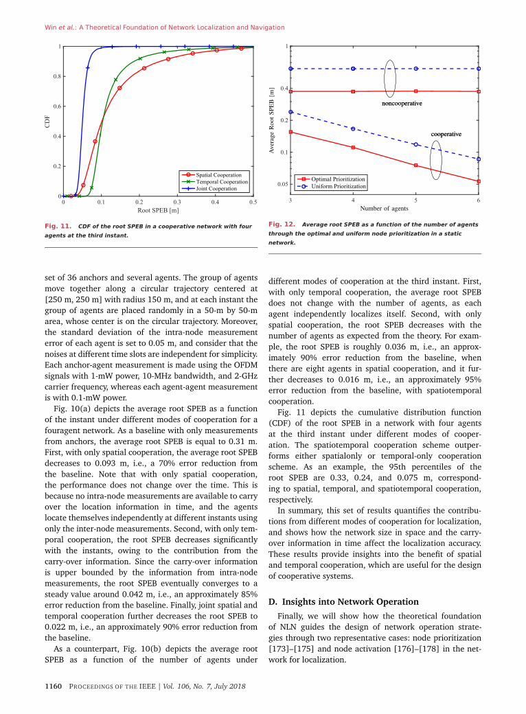
Win et al.: A Theoretical Foundation of Network Localization and Navigation
Fig. 11. CDF of the root SPEB in a cooperative network with four
agents at the third instant.
set of 36 anchors and several agents. The group of agentsmove together along a circular trajectory centered at[250 m, 250 m] with radius 150 m, and at each instant thegroup of agents are placed randomly in a 50-m by 50-marea, whose center is on the circular trajectory. Moreover,the standard deviation of the intra-node measurementerror of each agent is set to 0.05 m, and consider that thenoises at different time slots are independent for simplicity.Each anchor-agent measurement is made using the OFDMsignals with 1-mW power, 10-MHz bandwidth, and 2-GHzcarrier frequency, whereas each agent-agent measurementis with 0.1-mW power.
Fig. 10(a) depicts the average root SPEB as a functionof the instant under different modes of cooperation for afouragent network. As a baseline with only measurementsfrom anchors, the average root SPEB is equal to 0.31 m.First, with only spatial cooperation, the average root SPEBdecreases to 0.093 m, i.e., a 70% error reduction fromthe baseline. Note that with only spatial cooperation,the performance does not change over the time. This isbecause no intra-node measurements are available to carryover the location information in time, and the agentslocate themselves independently at different instants usingonly the inter-node measurements. Second, with only tem-poral cooperation, the root SPEB decreases significantlywith the instants, owing to the contribution from thecarry-over information. Since the carry-over informationis upper bounded by the information from intra-nodemeasurements, the root SPEB eventually converges to asteady value around 0.042 m, i.e., an approximately 85%error reduction from the baseline. Finally, joint spatial andtemporal cooperation further decreases the root SPEB to0.022 m, i.e., an approximately 90% error reduction fromthe baseline.
As a counterpart, Fig. 10(b) depicts the average rootSPEB as a function of the number of agents under
Fig. 12. Average root SPEB as a function of the number of agents
through the optimal and uniform node prioritization in a static
network.
different modes of cooperation at the third instant. First,with only temporal cooperation, the average root SPEBdoes not change with the number of agents, as eachagent independently localizes itself. Second, with onlyspatial cooperation, the root SPEB decreases with thenumber of agents as expected from the theory. For exam-ple, the root SPEB is roughly 0.036 m, i.e., an approx-imately 90% error reduction from the baseline, whenthere are eight agents in spatial cooperation, and it fur-ther decreases to 0.016 m, i.e., an approximately 95%error reduction from the baseline, with spatiotemporalcooperation.
Fig. 11 depicts the cumulative distribution function(CDF) of the root SPEB in a network with four agentsat the third instant under different modes of cooper-ation. The spatiotemporal cooperation scheme outper-forms either spatialonly or temporal-only cooperationscheme. As an example, the 95th percentiles of theroot SPEB are 0.33, 0.24, and 0.075 m, correspond-ing to spatial, temporal, and spatiotemporal cooperation,respectively.
In summary, this set of results quantifies the contribu-tions from different modes of cooperation for localization,and shows how the network size in space and the carry-over information in time affect the localization accuracy.These results provide insights into the benefit of spatialand temporal cooperation, which are useful for the designof cooperative systems.
D. Insights into Network Operation
Finally, we will show how the theoretical foundationof NLN guides the design of network operation strate-gies through two representative cases: node prioritization[173]–[175] and node activation [176]–[178] in the net-work for localization.
1160 PROCEEDINGS OF THE IEEE | Vol. 106, No. 7, July 2018

Win et al.: A Theoretical Foundation of Network Localization and Navigation
The goal of node prioritization is to achieve the bestlocalization accuracy for a given total transmission poweror bandwidth. In particular, for the static scenario, theproblem translates to allocating the total transmissionpower to anchors so that the average SPEB of the agents isminimized. The optimal solution for the node prioritizationcan be achieved by convex optimization programs thanksto the amenable properties of the SPEB [173]. As a base-line for comparison, we also adopt the uniform powerallocation. The signal bandwidth is 10 MHz, and the totalpower to be allocated among anchors is Na mW, andin the cooperative case each agent-agent ranging mea-surement consumes additional 0.1 mW. Fig. 12 depictsthe average root SPEB of the agents as a function ofthe number of agents. First, in the cooperative case, theaverage root SPEB decreases with the number of agentssince more degrees of freedom are available for nodeprioritization and additional agent-agent measurementsare available. Second, the optimal prioritization yields amuch better localization performance than the uniformprioritization. For example, in the noncooperative case,the former is 0.37 m while the latter is 0.61 m, whichconstitutes an approximately 40% error reduction. Third,the spatial cooperation among the agents further improvesthe localization performance with the same amount of totalpower from the anchors. For the case of four agents incooperation, the root SPEB reduces to 0.11 and 0.17 mwith the optimal and uniform prioritization, both yieldingan approximately 70% error reduction from their noncoop-erative counterparts. We also present the node activationas an example for the dynamic scenarios. The goal of nodeactivation is to select the best pairs of nodes for inter-node measurements at each instant so that the localizationerror of the entire network is minimized. The solution fornode activation can be obtained either by opportunisticactivation or by simply random activation with differenttradeoffs between the performance and communicationoverheads [176].23 Fig. 13 depicts the average root SPEBof the agents as a function of the number of measure-ment pairs at each instant, where the network has twoor six agents and the standard deviation of the intra-node measurement error of each agent is set to 0.05 m.Moreover, for a fair comparison, the total transmissionpower of the network is fixed to be Na mW, and thusmore measurement pairs result in less signal power foreach measurement pair. First, the average root SPEBdecreases with the number of measurement pairs for bothopportunistic and random activation as expected, sincemore degrees of freedom are available for node activationalthough the total transmission power is fixed. However,the additional gain diminishes as the number of measure-ment pairs grows, since the degree of freedom is fullyexploited. Second, the opportunistic activation can achieve
23The opportunistic activation selects the best set of links forreducing the SPEB at each instant, while the random activation selectsa number of links from available measurement pairs uniformly.
Fig. 13. Average root SPEB through the opportunistic and random
activation in a dynamic network. The network consists of two or six
agents that are randomly placed in the area.
a much better performance than its random counterparts.For instance, for the case of six agents in the networkemploying five measurement pairs at each instant, the rootSPEB is 0.069 and 0.293 m for opportunistic and randomactivation, respectively. That is, a 75% reduction in theroot SPEB can be achieved by the former method. Third,the opportunistic activation can yield better localizationperformance when there are more agents in the networkwith sufficient measurement links. In this case, mobileagents will not only have more opportunities to accessanchors, but also increase the diversity for selecting nodes,both of which can potentially provide more information forlocalization.
In summary, these results demonstrate that theoptimized node prioritization and node activation cansignificantly improve the localization performance underresource constraints. Meanwhile, with the aid of the the-oretical results, we can optimize the performance of thelocationaware networks in an efficient way.
VIII. C O N C L U S I O N
Location awareness is a key enabler for mobile networkapplications, spanning from location-based services toautonomous vehicles, which require different levels oflocalization accuracy and reliability. Network localizationand navigation (NLN) enabled by spatiotemporal coopera-tion is a promising paradigm that can dramatically improvethe localization performance. This paper presented a com-prehensive exploration of theoretical foundation, wherethe methodology of equivalent Fisher information analysiswas applied to determine the fundamental limits of local-ization accuracy attainable by spatiotemporal cooperation.The effects of spatiotemporal cooperation, the antennaarrays, and map exploitation were characterized on thelocalization performance, and a geometric interpretation
Vol. 106, No. 7, July 2018 | PROCEEDINGS OF THE IEEE 1161

Win et al.: A Theoretical Foundation of Network Localization and Navigation
was developed to visualize the information dynamicsin NLN. These results and the insights can be used to guidethe algorithm and network design for NLN.
Despite the recent advances in the field, there arestill several open challenges to be addressed for NLN. Inparticular, low-cost solutions for information fusion needto be developed for high-accuracy localization in harshenvironments. Also needed is the design of efficient com-munication protocols that can guarantee the efficiency and
reliability of NLN. In addition, security and privacy arecritical issues especially for homeland security and militaryapplications, which needs further study. �
IX. A C K N O W L E D G M E N T
The authors would like to thank A. Conti, G. C. Ferrante,A. Giorgetti, Z. Liu, and S. Mazuelas for their helpfulsuggestions and careful reading of the manuscript.
R E F E R E N C E S[1] M. Z. Win et al., “Network localization and
navigation via cooperation,” IEEE Commun. Mag.,vol. 49, no. 5, pp. 56–62, May 2011.
[2] N. Bulusu, J. Heidemann, and D. Estrin, “GPS-lesslow-cost outdoor localization for very smalldevices,” IEEE Pers. Commun., vol. 7, no. 5,pp. 28–34, Oct. 2000.
[3] D. Schneider, “New indoor navigationtechnologies work where GPS can’t,” IEEESpectrum, Nov. 2013.
[4] S. Gezici et al., “Localization via ultra-widebandradios: A look at positioning aspects for futuresensor networks,” IEEE Signal Process. Mag.,vol. 22, no. 4, pp. 70–84, Jul. 2005.
[5] Y. Shen and M. Z. Win, “Fundamental limits ofwideband localization—Part I: A generalframework,” IEEE Trans. Inf. Theory, vol. 56,no. 10, pp. 4956–4980, Oct. 2010.
[6] H. Godrich, A. M. Haimovich, and R. S. Blum,“Target localization accuracy gain in MIMOradar-based systems,” IEEE Trans. Inf. Theory,vol. 56, no. 6, pp. 2783–2803, Jun. 2010.
[7] B. T. Robinson, “Who goes there?” IEEE Spectrum,vol. 40, no. 10, pp. 42–47, Oct. 2003.
[8] F. Gustafsson and F. Gunnarsson, “Mobilepositioning using wireless networks: Possibilitiesand fundamental limitations based on availablewireless network measurements,” IEEE SignalProcess. Mag., vol. 22, no. 4, pp. 41–53, Jul. 2005.
[9] E. Paolini, A. Giorgetti, M. Chiani, R. Minutolo,and M. Montanari, “Localization capability ofcooperative anti-intruder radar systems,” EURASIPJ. Adv. Signal Process., vol. 2008, p. 726854,Dec. 2008.
[10] J. J. Caffery and G. L. Stüber, “Overview ofradiolocation in CDMA cellular systems,” IEEECommun. Mag., vol. 36, no. 4, pp. 38–45,Apr. 1998.
[11] K. Pahlavan, X. Li, and J.-P. Mäkelä, “Indoorgeolocation science and technology,” IEEECommun. Mag., vol. 40, no. 2, pp. 112–118,Feb. 2002.
[12] K. Yu, J.-P. Montillet, A. Rabbachin, P. Cheong, andI. Oppermann, “UWB location and tracking forwireless embedded networks,” Signal Process.,vol. 86, no. 9, pp. 2153–2171, 2006.
[13] J. Warrior, E. McHenry, and K. McGee, “Theyknow where you are—Location detection,” IEEESpectrum, vol. 40, no. 7, pp. 20–25, 2003.
[14] L.-J. Kau and C.-S. Chen, “A smart phone-basedpocket fall accident detection, positioning, andrescue system,” IEEE J. Biomed. Health Inf.,vol. 19, no. 1, pp. 44–56, Jan. 2015.
[15] T. Latif, E. Whitmire, T. Novak, and A. Bozkurt,“Sound localization sensors for search and rescuebiobots,” IEEE Sensors J., vol. 16, no. 10,pp. 3444–3453, May 2016.
[16] J. Guivant, E. Nebot, and S. Baiker, “Autonomousnavigation and map building using laser rangesensors in outdoor applications,” J. Robotic Syst.,vol. 17, no. 10, pp. 565–583, 2000.
[17] S.-H. Lee and C. C. Chung, “Robust multirateon-road vehicle localization for autonomoushighway driving vehicles,” IEEE Trans. ControlSyst. Technol., vol. 25, no. 2, pp. 577–589,Mar. 2017.
[18] G. Bresson, Z. Alsayed, L. Yu, and S. Glaser,“Simultaneous localization and mapping: A survey
of current trends in autonomous driving,” IEEETrans. Intell. Vehicles, vol. 2, no. 3, pp. 194–220,Sep. 2017.
[19] D. Miorandi, S. Sicari, F. D. Pellegrini, andI. Chlamtac, “Internet of Things: Vision,applications and research challenges,” Ad HocNetw., vol. 10, no. 7, pp. 1497–1516, Sep. 2012.
[20] L. Geng, M. F. Bugallo, A. Athalye, and P. M.Djuric, “Indoor tracking with RFID systems,” IEEEJ. Sel. Topics Signal Process., vol. 8, no. 1,pp. 96–105, Feb. 2014.
[21] F. Meyer, B. Etzlinger, Z. Liu, F. Hlawatsch, andM. Z. Win, “A scalable algorithm for networklocalization and synchronization,” IEEE InternetThings J., vol. 5, 2018, to appear.
[22] T. Budinger, “Biomonitoring with wirelesscommunications,” Annu. Rev. Biomed. Eng., vol. 5,no. 1, pp. 383–412, 2003.
[23] K. Witrisal et al., “High-accuracy localization forassisted living: 5G systems will turn multipathchannels from foe to friend,” IEEE Signal Process.Mag., vol. 33, no. 2, pp. 59–70, Mar. 2016.
[24] F. Buccafurri, G. Lax, S. Nicolazzo, and A. Nocera,“Robust multirate on-road vehicle localization forautonomous highway driving vehicles,” IEEETrans. Serv. Comput., to be published.
[25] F. Zabini and A. Conti, “Inhomogeneous Poissonsampling of finite-energy signals withuncertainties in R
d , ” IEEE Trans. Signal Process.,vol. 64, no. 18, pp. 4679–4694, Sep. 2016.
[26] G. Cardone et al., “Fostering participaction insmart cities: A geo-social crowdsensing platform,”IEEE Commun. Mag., vol. 51, no. 6, pp. 112–119,Jun. 2013.
[27] S. Bartoletti, A. Conti, and M. Z. Win, “Device-freecounting via wideband signals,” IEEE J. Sel. AreasCommun., vol. 35, no. 5, pp. 1163–1174,May. 2017.
[28] B. W. Parkinson and J. J. Spilker, Eds., GlobalPositioning System: Theory & Applications(Progress in Astronautics & Aeronautics), vol. 1.Washington, DC, USA: AIAA, 1996.
[29] B. W. Parkinson and J. J. Spilker, Eds., GlobalPositioning System: Theory and Applications(Progress in Astronautics and Aeronautics), vol. 2.Washington, DC, USA: AIAA 1996.
[30] J. J. Spilker, Jr., “GPS signal structure andperformance characteristics,” Navigation, vol. 25,no. 2, pp. 121–146, Aug. 1978.
[31] B. W. Parkinson and S. W. Gilbert, “NAVSTAR:Global positioning system—Ten years later,” Proc.IEEE, vol. 71, no. 10, pp. 1177–1186, Oct. 1983.
[32] E. Kaplan, Ed., Understanding GPS: Principles andApplications. Norwood, MA, USA: Artech House,1996.
[33] B. S. Pervan, D. G. Lawrence, and B. W. Parkinson,“Autonomous fault detection and removal usingGPS carrier phase,” IEEE Trans. Aerosp. Electron.Syst., vol. 34, no. 3, pp. 897–906, Jul. 1998.
[34] C. J. Hegarty and E. Chatre, “Evolution of theglobal navigation satellite system (GNSS),” Proc.IEEE, vol. 96, no. 12, pp. 1902–1917, Dec. 2008.
[35] R. W. Klukas, G. Lachapelle, C. Ma, and G.-I. Jee,“GPS signal fading model for urban centres,” IEEProc. Microw. Antennas Propag., vol. 150, no. 4,pp. 245–252, Aug. 2003.
[36] U. A. Khan, S. Kar, and J. M. F. Moura, “DILAND:An algorithm for distributed sensor localization
with noisy distance measurements,” IEEE Trans.Signal Process., vol. 58, no. 3, pp. 1940–1947,Mar. 2010.
[37] A. J. Weiss and A. Amar, “Direct positiondetermination of multiple radio signals,” EURASIPJ. Adv. Signal Process., vol. 2005, p. 653549,Dec. 2005.
[38] S. Bartoletti, W. Dai, A. Conti, and M. Z. Win, “Amathematical model for wideband ranging,” IEEEJ. Sel. Topics Signal Process., vol. 9, no. 2,pp. 216–228, Mar. 2015.
[39] K. Plarre and P. R. Kumar, “Tracking objects withnetworked scattered directional sensors,”EURASIP J. Adv. Signal Process., vol. 2008,p. 360912, Dec. 2008.
[40] P. Tichavský, C. H. Muravchik, and A. Nehorai,“Posterior Cramér-Rao bounds for discrete-timenonlinear filtering,” IEEE Trans. Signal Process.,vol. 46, no. 5, pp. 1386–1396, May 1998.
[41] S. Safavi, U. Khan, S. Kar, and J. Moura,“Distributed localization: A linear theory,” Proc.IEEE, vol. 106, no. 7, pp. 1204–1223, Jul. 2018.
[42] A. M. Haimovich, R. S. Blum, and L. J. Cimini,“MIMO radar with widely separated antennas,”IEEE Signal Process. Mag., vol. 25, no. 1,pp. 116–129, Jan. 2008.
[43] T. V. Nguyen, Y. Jeong, H. Shin, and M. Z. Win,“Machine learning for wideband localization,”IEEE J. Sel. Areas Commun., vol. 33, no. 7,pp. 1357–1380, Jul. 2015.
[44] H. Godrich, A. P. Petropulu, and H. V. Poor, “Powerallocation strategies for target localization indistributed multiple-radar architectures,” IEEETrans. Signal Process., vol. 59, no. 7,pp. 3226–3240, Jul. 2011.
[45] Y. Liu, Y. Shen, D. Guo, and M. Z. Win, “Networklocalization and synchronization using full-duplexradios,” IEEE Trans. Signal Process., vol. 66, no. 3,pp. 714–728, Feb. 2018.
[46] D. M. Bevly and B. Parkinson, “Cascaded Kalmanfilters for accurate estimation of multiple biases,dead-reckoning navigation, and full statefeedback control of ground vehicles,” IEEE Trans.Control Syst. Technol., vol. 15, no. 2, pp. 199–208,Mar. 2007.
[47] M. Rabinowitz and J. J. Spilker, “A newpositioning system using televisionsynchronization signals,” IEEE Trans. Broadcast.,vol. 51, no. 1, pp. 51–61, Mar. 2005.
[48] P. Tseng, “Second-order cone programmingrelaxation of sensor network localization,”.SIAM J.Optim., vol. 18, no. 1, pp. 156–185, Feb. 2007.
[49] S. Bartoletti, A. Giorgetti, M. Z. Win, and A. Conti,“Blind selection of representative observations forsensor radar networks,” IEEE Trans. Veh. Technol.,vol. 64, no. 4, pp. 1388–1400, Apr. 2015.
[50] O. Bialer, D. Raphaeli, and A. J. Weiss, “Two-waylocation estimation with synchronized basestations,” IEEE Trans. Signal Process., vol. 64,no. 10, pp. 2513–2527, May 2016.
[51] H. Chen, G. Wang, Z. Wang, H. C. So, andH. V. Poor, “Non-line-of-sight node localizationbased on semi-definite programming in wirelesssensor networks,” IEEE Trans. Wireless Commun.,vol. 11, no. 1, pp. 108–116, Jan. 2018.
[52] T. Tirer and A. J. Weiss, “Performance analysis of ahigh-resolution direct position determinationmethod,” IEEE Trans. Signal Process., vol. 65,
1162 PROCEEDINGS OF THE IEEE | Vol. 106, No. 7, July 2018

Win et al.: A Theoretical Foundation of Network Localization and Navigation
no. 3, pp. 544–554, Feb. 2017.[53] F. Meyer et al., “Message passing algorithms for
scalable multitarget tracking,” Proc. IEEE,vol. 106, no. 2, pp. 221–259, Feb. 2018.
[54] Y. Shen, H. Wymeersch, and M. Z. Win,“Fundamental limits of widebandlocalization—Part II: Cooperative networks,” IEEETrans. Inf. Theory, vol. 56, no. 10, pp. 4981–5000,Oct. 2010.
[55] Y. Shen, S. Mazuelas, and M. Z. Win, “Networknavigation: Theory and interpretation,” IEEE J.Sel. Areas Commun., vol. 30, no. 9,pp. 1823–1834, Oct. 2012.
[56] H. Wymeersch, J. Lien, and M. Z. Win,“Cooperative localization in wireless networks,”Proc. IEEE, vol. 97, no. 2, pp. 427–450, Feb. 2009.
[57] N. Patwari, J. N. Ash, S. Kyperountas, A. O. Hero,R. L. Moses, and N. S. Correal, “Locating thenodes: Cooperative localization in wireless sensornetworks,” IEEE Signal Process. Mag., vol. 22,no. 4, pp. 54–69, Jul. 2005.
[58] A. Conti, D. Dardari, M. Guerra, L. Mucchi, andM. Z. Win, “Experimental characterization ofdiversity navigation,” IEEE Syst. J., vol. 8, no. 1,pp. 115–124, Mar. 2014.
[59] H. Wymeersch, S. Marano, W. M. Gifford, andM. Z. Win, “A machine learning approach toranging error mitigation for UWB localization,”IEEE Trans. Commun., vol. 60, no. 6,pp. 1719–1728, Jun. 2012.
[60] J. Xu, X. Shen, J. W. Mark, and J. Cai, “Mobilelocation estimation in CDMA cellular networks byusing fuzzy logic,” Wireless Commun. MobileComput., vol. 7, no. 3, pp. 285–298, Mar. 2007.
[61] D. Dardari, A. Conti, U. Ferner, A. Giorgetti, andM. Z. Win, “Ranging with ultrawide bandwidthsignals in multipath environments,” Proc. IEEE,vol. 97, no. 2, pp. 404–426, Feb. 2009.
[62] B. Denis, J.-B. Pierrot, and C. Abou-Rjeily, “Jointdistributed synchronization and positioning inUWB ad hoc networks using TOA,” IEEE Trans.Microw. Theory Techn., vol. 54, no. 4,pp. 1896–1911, Jun. 2006.
[63] S. Mazuelas, A. Conti, J. C. Allen, and M. Z. Win,“Soft range information for network localization,”IEEE Trans. Signal Process., vol. 66, no. 12,pp. 3155–3168, Jun. 2018.
[64] A. Ohya, A. Kosaka, and A. Kak, “Vision-basednavigation by a mobile robot with obstacleavoidance using single-camera vision andultrasonic sensing,” IEEE Trans. Robot. Autom.,vol. 14, no. 6, pp. 969–978, Dec. 1998.
[65] J. A. Castellanos, J. Neira, and J. D. Tardos,“Multisensor fusion for simultaneous localizationand map building,” IEEE Trans. Robot. Autom.,vol. 17, no. 6, pp. 908–914, Dec. 2001.
[66] A. I. Mourikis, N. Trawny, S. I. Roumeliotis,A. E. Johnson, A. Ansar, and L. Matthies,“Vision-Aided Inertial Navigation for SpacecraftEntry, Descent, and Landing,” IEEE Trans. Robot.,vol. 25, no. 2, pp. 264–280, Apr. 2009.
[67] W. Burgard, O. Brock, and C. Stachniss,“Map-based precision vehicle localization in urbanenvironments,” in Proc. Robot. Sci. Syst. Conf.,Baden-Baden, Germany, Jun. 2007, pp. 121–128.
[68] J. Levinson et al., “Towards fully autonomousdriving: Systems and algorithms,” in Proc. IEEEIntell. Vehicles Symp. (IV), Baden-Baden, Germany,Jun. 2011, pp. 163–168.
[69] R. W. Wolcott and R. M. Eustice, “Visuallocalization within LIDAR maps for automatedurban driving,” in Proc. IEEE/RSJ Int. Conf. Intell.Robots Syst., Chicago, IL, USA, Sep. 2014,pp. 176–183.
[70] P. Lazik, N. Rajagopal, O. Shih, B. Sinopoli, andA. Rowe, “ALPS: A Bluetooth and ultrasoundplatform for mapping and localization,” in Proc.Conf. Embedded Networked Sensor Syst., Seoul,South Korea, 2015, pp. 73–84.
[71] N. B. Priyantha, A. Chakraborty, andH. Balakrishnan, “The cricket location-supportsystem,” in Proc. 6th Annu. Int. Conf. MobileComput. Netw. New York, NY, USA: 2000,pp. 32–43.
[72] Z. Liu, W. Dai, and M. Z. Win, “Mercury: An
infrastructure-free system for network localizationand navigation,” IEEE Trans. Mobile Comput.,vol. 17, no. 5, pp. 1119–1133, May 2018.
[73] U. A. Khan, S. Kar, and J. M. F. Moura,“Distributed sensor localization in randomenvironments using minimal number of anchornodes,” IEEE Trans. Signal Process., vol. 57, no. 5,pp. 2000–2016, May 2009.
[74] M. Z. Win and Y. Shen, “On the accuracy oflocalization systems using wideband antennaarrays,” IEEE Trans. Commun., vol. 58, no. 1,pp. 270–280, Jan. 2010.
[75] A. H. Sayed, A. Tarighat, and N. Khajehnouri,“Network-based wireless location: Challengesfaced in developing techniques for accuratewireless location information,” IEEE SignalProcess. Mag., vol. 22, no. 4, pp. 24–40, Jul. 2005.
[76] J. Prieto, S. Mazuelas, and M. Z. Win,“Context-aided inertial navigation via beliefcondensation,” IEEE Trans. Signal Process., vol. 64,no. 12, pp. 3250–3261, Jun. 2016.
[77] P. D. Groves, Principles of GNSS, Inertial, andMultisensor Integrated Navigation Systems.Norwood, MA, USA: Artech House, 2008.
[78] A. R. J. Ruiz, F. S. Granja, J. C. P. Honorato, andJ. I. G. Rosas, “Accurate pedestrian indoornavigation by tightly coupling foot-mounted IMUand RFID measurements,” IEEE Trans. Instrum.Meas., vol. 61, no. 1, pp. 178–189, Jan. 2012.
[79] S. Beauregard, “A helmet-mounted pedestriandead reckoning system,” in Proc. 3rd Int. ForumAppl. Wearable Comput., Mar. 2006, pp. 1–11.
[80] S. Mazuelas, Y. Shen, and M. Z. Win, “Beliefcondensation filtering,” IEEE Trans. Signal Process.,vol. 61, no. 18, pp. 4403–4415, Sep. 2013.
[81] E. Foxlin, “Pedestrian tracking with shoe-mountedinertial sensors,” IEEE Comput. Graph. Appl.,vol. 25, no. 6, pp. 38–46, Nov./Dec. 2005.
[82] J. Wolf, W. Burgard, and H. Burkhardt, “Robustvision-based localization by combining animage-retrieval system with Monte Carlolocalization,” IEEE Trans. Robot., vol. 21, no. 2,pp. 208–216, Apr. 2005.
[83] S. Se, D. G. Lowe, and J. J. Little, “Vision-basedglobal localization and mapping for mobilerobots,” IEEE Trans. Robot., vol. 21, no. 3,pp. 364–375, Jun. 2005.
[84] A. J. Davison and D. W. Murray, “Simultaneouslocalization and map-building using active vision,”IEEE Trans. Pattern Anal. Mach. Intell., vol. 24,no. 7, pp. 865–880, Jul. 2002.
[85] A. Georgiev and P. K. Allen, “Localization methodsfor a mobile robot in urban environments,” IEEETrans. Robot., vol. 20, no. 5, pp. 851–864,Oct. 2004.
[86] A. Conti, M. Guerra, D. Dardari, N. Decarli, andM. Z. Win, “Network experimentation forcooperative localization,” IEEE J. Sel. AreasCommun., vol. 30, no. 2, pp. 467–475, Feb. 2012.
[87] M. Anisetti, C. A. Ardagna, V. Bellandi, E.Damiani, and S. Reale, “Map-based location andtracking in multipath outdoor mobile networks,”IEEE Trans. Wireless Commun., vol. 10, no. 3,pp. 814–824, Mar. 2011.
[88] Y. Cheng and T. Singh, “Efficient particle filteringfor road-constrained target tracking,” IEEE Trans.Aerosp. Electron. Syst., vol. 43, no. 4,pp. 1454–1469, Oct. 2007.
[89] F. Montorsi, S. Mazuelas, G. M. Vitetta, andM. Z. Win, “On the performance limits ofmap-aware localization,” IEEE Trans. Inf. Theory,vol. 59, no. 8, pp. 5023–5038, Aug. 2013.
[90] K. Zhang, Y. Shen, and M. Z. Win, “On theperformance of map-aware cooperativelocalization,” in Proc. IEEE Int. Conf. Commun.,Kuala Lumpur, Malaysia, May 2016, pp. 1–6.
[91] C. Falsi, D. Dardari, L. Mucchi, and M. Z. Win,“Time of arrival estimation for UWB localizers inrealistic environments,” EURASIP J. Appl. SignalProcess., vol. 2006, Article ID 32 082, 2006.
[92] A. Rabbachin, I. Oppermann, and B. Denis, “GMLToA estimation based on low complexity UWBenergy detection,” in Proc. PIMRC, Helsinki,Finland, Sep. 2006, pp. 1–5.
[93] D. Dardari, C.-C. Chong, and M. Z. Win,
“Threshold-based time-of-arrival estimators inUWB dense multipath channels,” IEEE Trans.Commun., vol. 56, no. 8, pp. 1366–1378,Aug. 2008.
[94] Z. N. Low, J. H. Cheong, C. L. Law, W. T. Ng, andY. J. Lee, “Pulse detection algorithm forline-of-sight (LOS) UWB ranging applications,”IEEE Antennas Wireless Propag. Lett., vol. 4,pp. 63–67, 2005.
[95] Z. Zhang, C. L. Law, and Y. L. Guan,“BA-POC-based ranging method with multipathmitigation,” IEEE Antennas Wireless Propag. Lett.,vol. 4, no. 1, pp. 492–495, 2005.
[96] M. Leng, W. P. Tay, C. M. S. See, S. G. Razul, andM. Z. Win, “Modified CRLB for cooperativegeolocation of two devices using signals ofopportunity,” IEEE Trans. Wireless Commun.,vol. 13, no. 7, pp. 3636–3649, Jul. 2014.
[97] T. Wang, Y. Shen, S. Mazuelas, H. Shin, andM. Z. Win, “On OFDM ranging accuracy inmultipath channels,” IEEE Syst. J., vol. 8, no. 1,pp. 104–114, Mar. 2014.
[98] J. Caffery, Wireless Location in CDMA CellularRadio Systems. Boston, MA, USA: Kluwer, 2000.
[99] T. S. Rappaport, J. Reed, and B. D. Woerner,“Position location using wireless communicationson highways of the future,” IEEE Commun. Mag.,vol. 34, no. 10, pp. 33–41, Oct. 1996.
[100] W. W.-L. Li, Y. Shen, Y. J. Zhang, and M. Z. Win,“Robust power allocation for energy-efficientlocation-aware networks,” IEEE/ACM Trans. Netw.,vol. 21, no. 6, pp. 1918–1930, Dec. 2013.
[101] H.-S. Ahn and W. Yu, “Environmental-adaptiveRSSI-based indoor localization,” IEEE Trans.Autom. Sci. Eng., vol. 6, no. 4, pp. 626–633,Oct. 2009.
[102] N. Patwari and A. O. Hero, III, “Using proximityand quantized RSS for sensor localization inwireless networks,” Proc. IEEE/ACM 2nd WorkshopWireless Sensor Nets. Appl., 2003, pp. 20–29.
[103] T. Pavani, G. Costa, M. Mazzotti, A. Conti, andD. Dardari, “Experimental results on indoorlocalization techniques through wireless sensorsnetwork,” in Proc. IEEE Semiannu. Veh. Technol.Conf., vol. 2, Melbourne, Australia, May 2006,pp. 663–667.
[104] J. P. Beaudeau, M. F. Bugallo, and P. M. Djuric,“RSSI-based multi-target tracking by cooperativeagents using fusion of cross-target information,”IEEE Trans. Signal Process., vol. 63, no. 19,pp. 5033–5044, Oct. 2015.
[105] P. Bahl and V. N. Padmanabhan, “RADAR: Anin-building RF-based user location and trackingsystem,” in Proc. INFOCOM, vol. 2, Tel Aviv, Israel,Mar. 2000, pp. 775–784.
[106] Y. Shang, W. Rumi, Y. Zhang, and M. Fromherz,“Localization from connectivity in sensornetworks,” IEEE Trans. Parallel Distrib. Syst.,vol. 15, no. 11, pp. 961–974, Nov. 2004.
[107] T. He, C. Huang, B. M. Blum, J. A. Stankovic, andT. Abdelzaher, “Range-free localization schemesfor large scale sensor networks,” in Proc. 9thAnnu. Int. Conf. Mobile Comput. Netw., New York,NY, USA, 2003, pp. 81–95.
[108] M. Li and Y. Liu, “Rendered path: Range-freelocalization in anisotropic sensor networks withholes,” IEEE/ACM Trans. Netw., vol. 18, no. 1,pp. 320–332, Feb. 2010.
[109] T.-J. Shan, M. Wax, and T. Kailath, “On spatialsmoothing for direction-of-arrival estimation ofcoherent signals,” IEEE Trans. Acoust. SpeechSignal Process., vol. 33, no. 4, pp. 806–811,Apr. 1985.
[110] B. D. V. Veen and K. M. Buckley, “Beamforming: Aversatile approach to spatial filtering,” IEEE ASSPMag., vol. 5, no. 2, pp. 4–24, Apr. 1988.
[111] H. Krim and M. Viberg, “Two decades of arraysignal processing research: The parametricapproach,” IEEE Signal Process. Mag., vol. 13,no. 4, pp. 67–94, Jul. 1996.
[112] R. Engelbrecht, “Passive source localization fromspatially correlated angle-of-arrival data,” IEEETrans. Acoust. Speech Signal Process., vol. 31,no. 4, pp. 842–846, Aug. 1983.
[113] M. Wax and T. Kailath, “Optimum localization of
Vol. 106, No. 7, July 2018 | PROCEEDINGS OF THE IEEE 1163

Win et al.: A Theoretical Foundation of Network Localization and Navigation
multiple sources by passive arrays,” IEEE/ACMTrans. Audio Speech Language Process., vol. 31,no. 5, pp. 1210–1217, Oct. 1983.
[114] R. Roy and T. Kailath, “ESPRIT-estimation of signalparameters via rotational invariance techniques,”IEEE/ACM Trans. Audio Speech Language Process.,vol. 37, no. 7, pp. 984–995, Jul. 1989.
[115] C.-C. Chong, C.-M. Tan, D. I. Laurenson,S. McLaughlin, M. A. Beach, and A. R. Nix, “A newstatistical wideband spatio-temporal channelmodel for 5-GHz band WLAN systems,” IEEE J.Sel. Areas Commun., vol. 21, no. 2, pp. 139–150,Feb. 2003.
[116] D. Niculescu and B. Nath, “Ad hoc positioningsystem (APS) using AOA,” in Proc. 22nd Annu.Joint Conf. IEEE Comput. Commun., vol. 3. SanFrancisco, CA, USA, Mar./Apr. 2003,pp. 1734–1743.
[117] L. Xiong, “A selective model to suppress NLOSsignals in angle-of-arrival (AOA) locationestimation,” in Proc. 9th IEEE Int. Symp. Pers.Indoor Mobile Radio Commun., vol. Sep. 1, 1998,pp. 461–465.
[118] H.-J. Shao, X.-P. Zhang, and Z. Wang, “Efficientclosed-form algorithms for AOA basedself-localization of sensor nodes using auxiliaryvariables,” IEEE Trans. Signal Process., vol. 62,no. 10, pp. 2580–2594, May 2014.
[119] A. F. Molisch, Wireless Communications, 1st ed.Piscataway, NJ, USA: Wiley, 2005.
[120] C.-Y. Lee, “Finding the approximate angularprobability density function of wave arrival byusing a directional antenna,” IEEE Trans. AntennasPropag., vol. 21, no. 3, pp. 328–334, May 1973.
[121] B. Zhang and F. Yu, “LSWD: Localization schemefor wireless sensor networks using directionalantenna,” IEEE Trans. Consum. Electron., vol. 56,no. 4, pp. 2208–2216, Nov. 2010.
[122] T. V. Nguyen, Y. Jeong, H. Shin, and M. Z. Win,“Least square cooperative localization,” IEEETrans. Veh. Technol., vol. 64, no. 4,pp. 1318–1330, Apr. 2015.
[123] J. Luo and Q. Zhang, “Relative distance basedlocalization for mobile sensor networks,” in Proc.IEEE Global Telecomm. Conf., DC, USA, Nov. 2007,pp. 1076–1080.
[124] J. Chen, W. Dai, Y. Shen, V. K. N. Lau, andM. Z. Win, “Resource management games fordistributed network localization,” IEEE J. Sel.Areas Commun., vol. 35, no. 2, pp. 317–329,Feb. 2017.
[125] S. Safavi and U. A. Khan, “An opportunisticlinear-convex algorithm for localization in mobilerobot networks,” IEEE Trans. Robot., vol. 33, no. 4,pp. 875–888, Aug. 2017.
[126] S. Safavi and U. A. Khan, “Localization in mobilenetworks via virtual convex hulls,” IEEE Trans.Signal Inf. Process. Netw., vol. 4, no. 1,pp. 188–201, Mar. 2018.
[127] W. Chen and X. Meng, “A cooperative localizationscheme for zigbee-based wireless sensornetworks,” in Proc. 14th IEEE Int. Conf. Netw.,Singapore, Sep. 2006, pp. 1–5.
[128] N. Alsindi and K. Pahlavan, “Cooperativelocalization bounds for indoor ultra-widebandwireless sensor networks,” EURASIP J. Adv. SignalProcess., vol. Jan. 2008, 2008, no. 125.
[129] C. Savarese, J. M. Rabaey, and J. Beutel,“Locationing in distributed ad-hoc wireless sensornetworks,” in Proc. IEEE Int. Conf. Acoust. SpeechSignal Process., vol. May 4. 2001, pp. 2037–2040.
[130] W. Dai, Y. Shen, and M. Z. Win, “Distributedpower allocation for cooperative wireless networklocalization,” IEEE J. Sel. Areas Commun., vol. 33,no. 1, pp. 28–40, Jan. 2015.
[131] X. Tan and J. Li, “Cooperative positioning inunderwater sensor networks,” IEEE Trans. SignalProcess., vol. 58, no. 11, pp. 5860–5871,Nov. 2010.
[132] R. M. Vaghefi, M. R. Gholami, R. M. Buehrer, andE. G. Ström, “Cooperative received signalstrength-based sensor localization with unknowntransmit powers,” IEEE Trans. Signal Process.,vol. 61, no. 6, pp. 1389–1403, Mar. 2013.
[133] J. Chen, W. Dai, Y. Shen, V. K. N. Lau, and
M. Z. Win, “Power management for cooperativelocalization: A game theoretical approach,” IEEETrans. Signal Process., vol. 64, no. 24,pp. 6517–6532, Dec. 2016.
[134] C. Chang and A. Sahai, “Cramér-Rao-type boundsfor localization,” EURASIP J. Appl. Signal Process.,vol. Dec. 2006, 2006, no. 094287.
[135] S. B. Cruz, T. E. Abrudan, Z. Xiao, N. Trigoni, andJ. Barros, “Neighbor-aided localization invehicular networks,” IEEE Trans. Intell. Transp.Syst., vol. 18, no. 10, pp. 2693–2702, Oct. 2017.
[136] J. Yao, A. T. Balaei, M. Hassan, N. Alam, andA. G. Dempster, “Improving cooperativepositioning for vehicular networks,” IEEE Trans.Veh. Technol., vol. 60, no. 6, pp. 2810–2823,Jul. 2011.
[137] U. A. Khan and J. M. F. Moura, “Distributing theKalman filter for large-scale systems,” IEEE Trans.Signal Process., vol. 56, no. 10, pp. 4919–4935,Oct. 2008.
[138] S. Mazuelas, Y. Shen, and M. Z. Win, “Informationcoupling in cooperative localization,” IEEECommun. Lett., vol. 15, no. 7, pp. 737–739,Jul. 2011.
[139] S. Mazuelas, Y. Shen, and M. Z. Win,“Spatio-temporal information coupling in networknavigation,” IEEE Trans. Inf. Theory, vol. 64, 2018,to appear.
[140] H. L. Van Trees and K. L. Bell, Detection Estimationand Modulation Theory, Part 1. New York, NY:Wiley, 1968.
[141] H. V. Poor, An Introduction to Signal Detection andEstimation, 2nd ed. New York, NY, USA:Springer-Verlag, 1994.
[142] T. M. Cover and J. A. Thomas, Elements ofInformation Theory, 2nd ed. Hoboken, NJ, USA:Wiley, 2006.
[143] F. Gini, R. Reggiannini, and U. Mengali, “Themodified Cramér–Rao bound in vector parameterestimation,” IEEE Trans. Commun., vol. 46, no. 1,pp. 52–60, Jan. 1998.
[144] I. Reuven and H. Messer, “A Barankin-type lowerbound on the estimation error of a hybridparameter vector,” IEEE Trans. Inf. Theory, vol. 43,no. 3, pp. 1084–1093, May 1997.
[145] J. Ziv and M. Zakai, “Some lower bounds onsignal parameter estimation,” IEEE Trans. Inf.Theory, vol. 15, no. 3, pp. 386–391, May. 1969.
[146] M. Zakai and J. Ziv, “On the threshold effect inradar range estimation,” IEEE Trans. Inf. Theory,vol. IT-15, no. 1, pp. 167–170, Jan. 1969.
[147] D. Chazan, M. Zakai, and J. Ziv, “Improved lowerbounds on signal parameter estimation,” IEEETrans. Inf. Theory, vol. 21, no. 1, pp. 90–93,Jan. 1975.
[148] K. L. Bell, Y. Steinberg, Y. Ephraim, and H. L. V.Trees, “Extended Ziv-Zakai lower bound for vectorparameter estimation,” IEEE Trans. Inf. Theory,vol. 43, no. 2, pp. 624–637, Mar. 1997.
[149] E. Weinstein and A. J. Weiss, “A general class oflower bounds in parameter estimation,” IEEETrans. Inf. Theory, vol. 34, no. 2, pp. 338–342,Mar. 1988.
[150] C. Chang and A. Sahai, “Estimation bounds forlocalization,” in Proc. IEEE Commun. Soc. Conf.Sensor Ad Hoc Commun. Netw. (SECON),Oct. 2004, pp. 415–424.
[151] L. Mailaender, “On the geolocation bounds forround-trip time-of-arrival and all non-line-of-sightchannels,” EURASIP J. Adv. Signal Process.,vol. Dec. 2008, 2008, no. 584670.
[152] Y. Qi, H. Kobayashi, and H. Suda, “Analysis ofwireless geolocation in a non-line-of-sightenvironment,” IEEE Trans. Wireless Commun.,vol. 5, no. 3, pp. 672–681, Mar. 2006.
[153] D. Jourdan, D. Dardari, and M. Win, “Positionerror bound for UWB localization in densecluttered environments,” IEEE Trans. Aerosp.Electron. Syst., vol. 44, no. 2, pp. 613–628,Apr. 2008.
[154] S. Venkatesh and R. M. Buehrer, “Multiple-accessinsights from bounds on sensor localization,”Pervasive Mobile Comput., vol. 4, no. 1, pp. 33–61,2008.
[155] S. Mazuelas, R. M. Lorenzo, A. Bahillo, P.
Fernandez, J. Prieto, and E. J. Abril, “Topologyassessment provided by weighted barycentricparameters in harsh environment wirelesslocation systems,” IEEE Trans. Signal Process.,vol. 58, no. 7, pp. 3842–3857, Jul. 2010.
[156] Y. Qi and H. Kobayashi, “Cramér-Rao lower boundfor geolocation in non-line-of-sight environment,”in Proc. IEEE Int. Conf. Acoust. Speech SignalProcess., Orlando, FL, USA, May 2002,pp. III-2473–III-2476.
[157] Y. Qi, H. Suda, and H. Kobayashi, “Ontime-of-arrival positioning in a multipathenvironment,” in Proc. IEEE Semiannu. Veh.Technol. Conf., Los Angeles, CA, USA, Sep. 2004,pp. 3540–3544.
[158] Y. Shen and M. Z. Win, “Fundamental limits ofwideband localization accuracy via Fisherinformation,” in Proc. IEEE Wireless Commun.Netw. Conf., Kowloon, China, Mar. 2007,pp. 3046–3051.
[159] Y. Han et al., “Performance limits and geometricproperties of array localization,” IEEE Trans. Inf.Theory, vol. 62, no. 2, pp. 1054–1075, Feb. 2016.
[160] O. Cappe, E. Moulines, and T. Ryden, Inference inHidden Markov Models, ser. Statistics. New York,NY, USA: Springer-Verlag, 2007.
[161] L. R. Rabiner, “A tutorial on hidden Markovmodels and selected applications in speechrecognition,” Proc. IEEE, vol. 77, no. 2,pp. 257–286, Feb. 1989.
[162] L. Rabiner and B. Juang, “An introduction tohidden Markov models,” IEEE ASSP Mag., vol. 3,no. 1, pp. 4–16, Jan. 1986.
[163] T. Kailath, A. H. Sayed, and B. Hassibi, LinearEstimation, ser. Information and System Sciences.Upper Saddle River, NJ, USA: Prentice-Hall,2000.
[164] S. Bay, B. Geller, A. Renaux, J.-P. Barbot, andJ.-M. Brossier, “On the hybrid Cramér Rao boundand its application to dynamical phaseestimation,” IEEE Wireless Commun. Lett., vol. 15,no. 8, pp. 453–456, May 2008.
[165] A. T. Ihler, J. W. Fisher, R. L. Moses, and A. S.Willsky, “Nonparametric belief propagation forself-localization of sensor networks,” IEEE J. Sel.Areas Commun., vol. 23, no. 4, pp. 809–819,Apr. 2005.
[166] J. Aspnes et al., “A theory of networklocalization,” IEEE Trans. Mobile Comput., vol. 5,no. 12, pp. 1663–1678, Dec. 2006.
[167] P. Biswas, T.-C. Lian, T.-C. Wang, and Y. Ye,“Semidefinite programming based algorithms forsensor network localization,” ACM Trans. SensorNetw., vol. 2, no. 2, pp. 188–220, 2006.
[168] S. Mazuelas, Y. Shen, and M. Z. Win,“Spatio-temporal information coupling incooperative navigation,” in Proc. IEEE GlobalTelecomm. Conf., Anaheim, CA, USA, Dec. 2012,pp. 2403–2407.
[169] Technical Specification LTE;Evolved UniversalTerrestrial Radio Access (E-UTRA); User Equipment(UE) Radio Transmission and Reception, documentTS 136.101 V11.2.0, 3rd Generation PartnershipProject, 3GPP, Nov. 2012.
[170] Technical Report LTE; 5G; Study on Channel Modelfor Frequency Spectrum Above 6 GHz, Release 14,document ETSI TR 138 900 V14.3.1, 3rdGeneration Partnership Project, 3GPP, Aug. 2017.
[171] F. Ademaj, M. K. Müller, S. Schwarz, and M. Rupp,“Modeling of spatially correlated geometry-basedstochastic channel,” in Proc. IEEE Semiannual Veh.Technol. Conf., Toronto, ON, Canada, Sep. 2017,pp. 1–6.
[172] S. Jaeckel, L. Raschkowski, K. Börner, L. Thiele,F. Burkhardt, and E. Eberlein, “Quasi deterministicradio channel generator user manual anddocumentation,” Fraunhofer Heinrich Hertz Inst.,Berlin, Germany, Tech. Rep., 2017.
[173] Y. Shen, W. Dai, and M. Z. Win, “Poweroptimization for network localization,” IEEE/ACMTrans. Netw., vol. 22, no. 4, pp. 1337–1350,Aug. 2014.
[174] W. Dai, Y. Shen, and M. Z. Win, “Energy-efficientnetwork navigation algorithms,” IEEE J. Sel. AreasCommun., vol. 33, no. 7, pp. 1418–1430,
1164 PROCEEDINGS OF THE IEEE | Vol. 106, No. 7, July 2018

Win et al.: A Theoretical Foundation of Network Localization and Navigation
Jul. 2015.[175] W. Dai, Y. Shen, and M. Z. Win, “A computational
geometry framework for efficient networklocalization,” IEEE Trans. Inf. Theory, vol. 64,no. 2, pp. 1317–1339, Feb. 2018.
[176] T. Wang, Y. Shen, A. Conti, and M. Z. Win,
“Network navigation with scheduling: Errorevolution,” IEEE Trans. Inf. Theory, vol. 63, no. 11,pp. 7509–7534, Nov. 2017.
[177] T. Wang, Y. Shen, A. Conti, and M. Z. Win,“Analysis of network navigation with schedulingstrategies,” in Proc. IEEE Int. Conf. Commun.,
London, U.K., Jun. 2015, pp. 3562–3566.[178] M. Z. Win, W. Dai, Y. Shen, G. Chrisikos, and
H. V. Poor, “Network operation strategies forefficient localization and navigation,” Proc. IEEE,vol. 106, no. 7, pp. 1224–1254, Jul. 2018.
A B O U T T H E A U T H O R S
Moe Z. Win (Fellow, IEEE) is a Professorat the Massachusetts Institute of Technology(MIT), Cambridge, MA, USA and the found-ing director of the Wireless Information andNetwork Sciences Laboratory. Prior to joiningMIT, he was with AT&T Research Laborato-ries and NASA Jet Propulsion Laboratory.His research encompasses fundamental
theories, algorithm design, and networkexperimentation for a broad range of real-world problems. Hiscurrent research topics include network localization and naviga-tion, network interference exploitation, and quantum informationscience. He has served the IEEE Communications Society as anelected Member-at-Large on the Board of Governors, as electedChair of the Radio Communications Committee, and as an IEEEDistinguished Lecturer. Over the last two decades, he held variouseditorial positions for IEEE journals and organized numerous inter-national conferences. Currently, he is serving on the SIAM DiversityAdvisory Committee.Dr. Win is an elected Fellow of the American Association for the
Advancement of Science (AAAS) and the Institution of Engineeringand Technology (IET). He was honored with two IEEE TechnicalField Awards: the IEEE Kiyo Tomiyasu Award (2011) and the IEEEEric E. Sumner Award (2006, jointly with R. A. Scholtz). Togetherwith students and colleagues, his papers have received numer-ous awards. Other recognitions include the IEEE CommunicationsSociety Edwin H. Armstrong Achievement Award (2016), the Inter-national Prize for Communications Cristoforo Colombo (2013), theCopernicus Fellowship (2011) and the Laurea Honoris Causa (2008)from the Universitá degli Studi di Ferrara, and the U.S. PresidentialEarly Career Award for Scientists and Engineers (2004). He is an ISIHighly Cited Researcher.
Yuan Shen (Member, IEEE) received theB.E. degree (with highest honor) in elec-tronic engineering from Tsinghua University,Beijing, China, in 2005 and the S.M. andPh.D. degrees in electrical engineering andcomputer science from the MassachusettsInstitute of Technology (MIT), Cambridge,MA, USA, in 2008 and 2014, respectively.He is an Associate Professor at the Depart-
ment of Electronic Engineering, Tsinghua University. Prior to that,he was a Research Assistant and then Postdoctoral Associate atthe Wireless Information and Network Sciences Laboratory, MIT, in2005–2014. He was with the Hewlett-Packard Labs in winter 2009and the Corporate R&D at Qualcomm Inc. in summer 2008. Hisresearch interests include statistical inference, network science,communication theory, information theory, and optimization. Hiscurrent research focuses on network localization and navigation,inference techniques, resource allocation, and intrinsic wirelesssecrecy.
Prof. Shen was a recipient of the Qiu Shi Outstanding YoungScholar Award (2015), the China’s Youth 1000-Talent Program(2014), the Marconi Society Paul Baran Young Scholar Award(2010), and the MIT Walter A. Rosenblith Presidential Fellowship(2005). His papers received the IEEE Communications Society FredW. Ellersick Prize (2012) and three Best Paper Awards from IEEEinternational conferences. He is an elected Vice Chair (2017–2018)and Secretary (2015–2016) for the IEEE ComSoc Radio Commu-nications Committee. He serves as TPC symposium Co-Chair forIEEE Globecom (2018 and 2016), the European Signal ProcessingConference (EUSIPCO 2016), and the IEEE ICC Advanced NetworkLocalization and Navigation (ANLN) Workshop (2016, 2017, and2018). He also serves as Editor for the IEEE TRANSACTIONS ON WIRELESS
COMMUNICATIONS (since 2018), IEEE COMMUNICATIONS LETERS (since 2015),and IEEE CHINA COMMUNICATIONS (since 2017), and served as GuestEditor for the International Journal of Distributed Sensor Networks(in 2015).
Wenhan Dai (Student Member, IEEE)received the B.S. degrees in electronic engi-neering and in mathematics from TsinghuaUniversity, Beijing, China, in 2011 and theS.M. degree in aeronautics and astronauticsfrom the Massachusetts Institute of Technol-ogy (MIT), Cambridge, MA, USA, in 2014,where he is currently working toward thePh.D. degree at the Wireless Information andNetwork Sciences Laboratory.His research interests include communication theory and sto-
chastic optimization with application to wireless communicationand network localization. His current research focuses on efficientnetwork localization, cooperative network operation, and ultraw-ideband communication.Mr. Dai was honored by the Marconi Society with the Paul Baran
Young Scholar Award (2017). He received the Marconi-BISITE BestPaper Award from the IEEE ICUWB (2017), the Chinese GovernmentAward for Outstanding Student Abroad (2016), the first prize of theIEEE Communications Society Student Competition (2016), and theStudent Paper Award (first place) from the IEEE CWIT (2015). Hewas recognized as the exemplary reviewer of IEEE CommunicationsLeters (2014).
Vol. 106, No. 7, July 2018 | PROCEEDINGS OF THE IEEE 1165