A theoretical and experimental study of the Broyden

Vol. 6(8), pp. 166-176, August, 2013

DOI: 10.5897/AJMCSR11.072

ISSN 2006-9731 ©2013 Academic Journals

http://www.academicjournals.org/AJMCSR

African Journal of Mathematics and Computer Science Research

Full Length Research Paper

A theoretical and experimental study of the Broyden-Fletcher-Goldfarb-Shano (BFGS) update

T. A. Adewale1 and B. I. Oruh2*

1Department of Industrial Mathematics, Adekunle Ajasin University, P. M. B. 1, Akungba – Akoko, Nigeria.

2Department of Mathematics/Statistics/Computer Science, Michael Okpara University of Agriculture, Umudike, Nigeria.

Accepted 10 May, 2013

This paper discusses theoretically the evolution of a conjugate direction algorithm for minimizing an arbitrary nonlinear, non quadratic function using Broyden-Fletcher-Goldfarb-Shano (BFGS) update in quasi-Newton Method. The updating rule is initialized by a Moore Penrose’s generalized inverse. Specifically, an approximation to the inverse Hessian is constructed and the updating rule for this approximation is imbedded in the BFGS update. Numerical experiments show that, using the proposed line search algorithm and the modified quasi-Newton algorithm for unconstrained problems are very competitive. This paper produces a new analysis that demonstrates that the BFGS method with a line

search is step q-superlinear convergent with assumption of linearly independent iterates. The

analysis assumes that the inverse Hessian approximations are positive definite and bounded asymptotically, which from computational experience, are of reasonable assumptions. Key words: Quasi-Newton method, Moore-Penrose generalized inverse, Broyden-Fletcher-Goldfarb-Shano (BFGS) update, superlinear convergence, conjugate directions, orthogonalization of matrices.

INTRODUCTION This paper is connected with interactions in the form:

Where and is a

scalar and it is the step length parameter chosen under

the condition min and is determined by:

𝛼𝑘 = ∇𝑓 𝑥0 ,𝑆𝑘

𝐵𝑆𝑘 ,𝑆𝑘 = ∇𝑓 𝑥0 ,𝑆𝑘

𝑃𝑘 ,𝑆𝑘 ,𝑘 = 0,1,…𝑛 − 1,

is the search direction, is the gradient vector

at . Each is intended to approximate inverse

Hessian at and is chosen to prevent divergence of

the sequence , f is assumed to be at least twice

continuously differentiable. Bea-Israel (1996) developed an iterative scheme which can be employed for inversion of the Hessian of the objective function to be minimized, namely;

where H is an n × n matrix, is an orthogonal matrix

and B0 is chosen to be the Moore-Penrose generalized

inverse of H and it is derived as follows (Altman, 1960; Bernet 1979, Demidovich 1981, Rao and Mitra 1971, Rao 1973): Let M and N be given positive definite matrices,

be non-zero Eigenvalues of with

respect to or of with respect

*Corresponding author. E-mail:[email protected].

to N, be Eigenvectors of with respect

to and be eigenvectors of with

respect to N. We can write H in the form:

𝐻 = 𝑀−1 𝜇1ℑ1𝜂1𝑇 +⋯+ 𝜇𝑛ℑ𝑛𝜂𝑛

𝑇 𝑁 (1)

and the more Penrose generalized inverse of H

as:

𝐻+𝑀𝑁 = 𝜇1

−1𝜂1ℑ1𝑇 + 𝜇2

−1ℑ2𝑇 + ⋯+ 𝜇𝑛

−1𝜂𝑛ℑ𝑛𝑇 (2)

We shall take:

(3)

In a previous paper, was taken to be the n × n

identity matrix since it satisfied the properties of .;

namely:

𝐻𝐵0 − 𝑃𝐻 < 1, . is is any valid matrix norm

𝐻0𝐵 − 𝑃𝐻 < 1.

We shall chose the Frobenius norm defined by:

𝐻 𝐹 = ℎ𝑖𝑗2

1

2, ℎ𝑖𝑗 i,j, = 1,2,..,n.. (4)

Being the entries of H and PH to be the matrix derived as follows:

Let us take where non-singular and real

is. That is the Hessian matrix at the initial point. Let us represent this by:

(5)

And leave unchanged the first two rows, from each

row, subtract the second row of multiplied by

a scalar The new matrix is:

, for i = 1,2. (6)

and

(7)

Observing that the first row of coincides with the

Adewale and Oruh 167

first row of and all the other rows of are linear

combinations of the rows of orthogonal to the first

row of and therefore the row of will also be

orthogonal to its first row, we chose the multiplier so

that the row of , from the third onwards are

orthogonal to the second row. In summary, this is equivalent to:

(8) or

(9) Whence,

(10)

From each ith row of

beginning with the second subtract the first row multiplied

by a scalar, dependent on the

number of the row we get the transformed matrix

given by:

(11)

We chose multiplier such that the first row of matrix

is orthogonal to the other rows of the matrix. We then have:

(12)

Whence,

(13) This process is continued until we get the matrix:

(14)

168 Afr. J. Math. Comput. Sci. Res. All the rows are orthogonal in pairs, that is, until:

(15)

The matrix has orthogonal row and it is,

therefore, not difficult to see that:

(16)

That is, a diagonal matrix. Also if H is a matrix with orthogonal columns, then:

(17)

Also, if a matrix H has orthogonal row/column it is sufficient to normalize each row/column to orthogonalize it (Barnet 1979; Demidovich 1981) That is:

(18)

is an orthogonal matrix, we shall next set:

(19)

and the iteration is defined by:

(20)

Since is an approximation to we intend to

improve upon this using the Broyden–Fletcher–Goldfarb (BFGS) update defined by:

(21)

That is,

(22)

Where

A major drawback to quasi-Newton method (other than the difficulty of obtaining analytical derivatives) is that the value of the objective function is guaranteed to be improved on each cycle only if the Hessian matrix of the

objective function, is positive definite.

is positive definite for strictly convex functions but

for general functions, quasi-Newton method may lead to

search directions diverging from the minimum of .

Recall that a real symmetric matrix is positive definite if all the Eigenvalues are positive. We shall, therefore need to demonstrate or present schemes for “forcing” positive definiteness on the approximate inverse Hessian.

Certain authors have proposed that the Hessian matrix be forced to be positive definite at each stage of the minimization. Himelblau, (1972) and Rao, (1978) devised a scheme of Eigenvalue analysis that guaranteed that an

estimate of the inverse, , would be positive definite.

Let B-1

be approximate to H(x), scale the matrix B-1

as follows:

(23)

Where is a diagonal matrix whose elements are:

(24)

That is, the positive square root of the absolute values of

the elements on the main diagonal of will

have all positive or negative ones on its main diagonal.

Because and are non singular and of

order n, the inverse of the product is the product of the inverses in reverse order, or:

That is:

(25)

Then can be calculated from the scaled matrix as:

(26)

We can express, in terms of the Eigenvalues

of and the Eigenvalues of the inverse matrix are

simply the inverse , of the Eigenvalues of the original

matrix. Therefore:

(27)

Where is the normalized Eigenvector corresponding to

the Eigenvalues . Instead of using , however,

is used:

(28)

in which any of is replaced by a small positive number,

so that BK can now be guaranteed positive definite if computed from:

(29)

This scheme described above shall be employed in this presentation. The second scheme that shall be employed in this study was due to Marquardt (1963); Levenberg (1994) and Goldfield et al. (1966). To ensure that the

estimate of was positive definite the above

named authors suggested the following computation scheme:

(30)

Where, is a positive constant such that

. Because the Eigenvalues of

are , Equation (30) guarantees that

is positive definite since use of an approximate

in Equation (30) in effect destroys negative small Eigenvalues of the approximation to the Hessian matrix.

Note that with sufficiently large, can overwhelm

and the minimization approach a steepest descent

search. A third scheme which is only good for mentioning in this study is due to Zwart (1969) but will not be employed in this investigation.

The main purpose of this paper is to better understand the computational and theoretical properties of the BFGS update in the context of basic line search and quasi-Newton methods for unconstrained optimization for the BFGS method. Ge and Powell (1983) proved, under a different set of assumptions from those of Conn et al. (1988a; 1988b; 1991), that the sequence of general

matrices converges, but not necessarily to . We

shall demonstrate that under the assumption of uniform linear independence of sequence of steps and boundedness and positive definiteness of the guaranteed matrices a new convergence analysis is possible. We presented computation experience with the BFGS update using a standard line search technique and quasi-Newton algorithms for small to medium size unconstrained optimization problems. Convergence analysis is undertaken and some brief conclusion and comments regarding future research were made.

COMPUTATIONAL RESULTS AND ALGORITHM In order to test the performance of quasi-Newton

Adewale and Oruh 169 (conjugate direction) method for unconstrained optimization using BFGS update we present and discuss some numerical experiments that were conducted. Minimization of the function after orthogonalization of the Hessian matrix using: i) The Broyden-Fletcher-Goldfarb-Shano (BFGS) Update ii) The Davidon-Fletcher-Powell (DFP) update, iii) The symmetric rank one update and, iv) Minimization of RsenBrock’s Banana-shape valley function using Lagrange’s reduction of quadratic forms in quasi-Newton (lagroqf q-n) method for comparism.

The line search is based on a cubic modelling of in the direction of search developed by the authors and the Quasi-Newton is determined using the New Line Search Technique (Rao, 1978; Walsh, 1968) to approximately minimize the function in the experimental set of questions. The frame works of these algorithms are presented below:

Algorithm Quasi-Newton method (line search)

Step 0: give an initial vector of independent variables,

an initial positive definite matrix and

. Set k (the interaction counter) = 0

Step 1: if a convergence criterion is achieved, then stop Step 2: Compute a quasi-Newton direction

if is safely positive definite, else

set where such that

as defined in Equations 23 to 29 or 30

such that is safely positive definite.

Step 3: find an acceptable step length using algorithm

(31) (Adewale, 2003; Demidovick, 1981):

Step 4: Set

Step 5: Compute the next inverse Hessian approximation

using the BFGS update

Step 6: Set and go to Step 1.

Error in the inverse Hessian approximation and uniform linear independence Definition

A sequence of vectors in is said to be

uniformly linearly independent if there exist

and nm such that, for each nm , one can choose n

distinct indices:

mkkkk n ...1 such that the minimum

singular value of the matrix

170 Afr. J. Math. Comput. Sci. Res.

n1

1

kk

k

S...

S

Snk

k

SS (31)

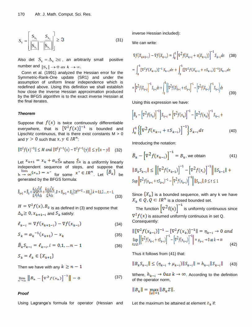
Also det kkS , an arbitrarily small positive

number and .0 kasSk

Conn et al. (1991) analyzed the Hessian error for the Symmetric-Rank-One update (SR1) and under the assumption of uniform linear independence which is redefined above. Using this definition we shall establish how close the inverse Hessian approximation produced by the BFGS algorithm is to the exact inverse Hessian at the final iterates.

Theorem

Suppose that is twice continuously differentiable

everywhere, that is is bounded and

Lipschitz continuous, that is there exist constants M > 0

and such that :

(32)

Let where is a uniformly linearly independent sequence of steps, and suppose that

for some . Let be generated by the BFGS formula:

(33)

is as defined in (3) and suppose that

and satisfy:

(34)

(35)

(36)

Then we have with any

(37)

Proof Using Lagrange’s formula for operator (Hessian and

inverse Hessian included): We can write:

(38)

(39) Using this expression we have:

(40)

Introducing the notation:

, we obtain (41)

Since is a bounded sequence, with any k we have

is a closed bounded set.

The function is uniformly continuous since

is assumed uniformly continuous in set Q.

Consequently:

(42) Thus it follows from (41) that:

(43)

Where, . According to the definition

of the operator norm,

Let the maximum be attained at element if:

(44)

Then because of the condition:

Where defined in (31), the

coefficients will be bounded, that is,

. Using (44) we obtain:

(45)

Hence by (43 and the fact that is bounded we

have:

That is:

and the theorem

is proved. Theorem

If is a continuously differentiable strongly convex

function and sequence is such that

and then .

Proof

According to condition we have:

with any . The

set is strongly convex since is a strongly convex

function. Then there is a positive number any

point , where , is an

internal point of the set . Let where

is a plane tangent to the set and

Then noting that: , we obtain

.

But µ since otherwise in addition to point

set and plane would have other point in

common, which contradicts the strong convexity of .

Adewale and Oruh 171 Therefore:

Hence, if . But

if , then since is strongly convex,

the maximum diameter of set which implies

that . The theorem is proved.

Theorem

If is a twice continuously differentiable function for

which

are valid, matrix with any is defined by

system of equations:

and satisfies the condition:

is determined to be

, then whatever the initial point the

following statement stated are valid for sequence:

and at a superlinear

rate of convergence, Where with any

COMPUTATIONAL RESULTS

On the basis of analogical heuristics, we shall implement the algorithm on four test problems, three of which are non quadratic functions common with authors of quasi-Newton methods. We shall orthogonalize the constant matrices resulting from the Hessian of the quadratic approximations to the function. They shall be compared under BFGS, SRL and DFP updates.

Problem

A quadratic function

𝐻 = 4 22 4

,𝐻 =

1 0

0 1

, 𝑧1 = 𝑥1

𝑧2 = 𝑥1 + 𝑥2 ,𝑓 𝑧 = 𝑧12 + 𝑧2

2 , 𝑧0 = (1,2)


Table 1. Minimization of Rosenbrock’s function (using the BFGS update).

0 101 104 18 8.6 × 10

-20

10-5

72 74 18 6.8 × 10-20

10

-3 60 61 17 1.6 × 10

-16

10-1

52 53 21 2.6 ×10-16

0.5 48 49 26 5.1 × 10

-18

0.75 40 42 32 2.8 × 10-20

0.9 40 42 32 2.8 ×10

-20

1.0 39 40 31 1.3 × 10-7

= Steplength parameter; = number of function evaluation; = error of function

value approximation; = number of iteration.

Table 2. minimization of Rosenbrock’s function using the DFP update.

0 118 119 22 3.7 × 10-20

10-5

88 89 22 3.4 × 10-20

10-3

77 78 22 5.8 × 10-20

10-1

61 63 24 1.3 × 10-20

0.5 59 60 29 1.1 × 10-17

0.75 41 42 36 2.1 × 10-19

0.9 45 46 35 8.2 × 10-20

1.0 41 42 35 2.7 ×10-18

= Steplength parameter; = number of function evaluation; = error

of function value approximation; = number of iteration.

Problem Powell’s quattic

𝑓 𝑋1 ,𝑋2 ,𝑋3,𝑋4 = 𝑋1 + 10𝑋2 2 + 5 𝑋3 − 𝑋4

2 + 𝑋2 − 2𝑋3 4 + 10 𝑥1 − 𝑋4

4

𝑋0 = 3,−1,0,1 𝑇 ,𝐻 =

4 0 0 0

0 10 0 0

0 0 2 0

0 0 0 20

. Problem Woods function

Problem Rosenbrock’s banana – shaped valley function

The numerical results are reported in Tables 1-11

including the Steplength parameter( , number of

function evaluation( ), error of function value

approximation( ), number of iteration( ). DISCUSSION OF COMPUTATIONAL RESULTS The BFGS update has appeared to be superior in general application. This finding was corroborated by S.H.C Dutoit when developing computer programs for the analysis of covariance structure arising from nonlinear growth curves and from autoregressive time series with moving average residual (Rao, 1978) In this presentation

Adewale and Oruh 173

Table 3. Minimization of Rosenbrock’s function using the symmetric-rank-one update (SR1).

0 128 4.9 × 10-17

130 23

10-5

97 5.2 × 10-17

99 23

10-3

83 6.0 × 10-17

84 23

10-1

67 1.9 × 10-21

69 27

0.5 56 6.2 × 10-16

56 30

0.75 53 1.8 ×10-14

54 35

0.9 55 2.1 × 10-15

56 41

1.0 55 2.1 × 10-20

57 44


value approximation; = number of iteration.

Table 4. Minimization of wood’s (using the BFGS update).

0 191 194 40 1.3 × 10-16

10-5

142 144 40 1.6 × 10-16

10-3

113 116 37 1.7 × 10-21

10-1

85 86 38 3.8 × 10-20

0.5 96 98 69 4.0 × 10-17

0.75 93 95 73 5.4 × 10-17

0.9 87 89 73 4.6 × 10-16

1.0 97 98 75 9.0 × 10-15

= Steplength parameter; = number of function evaluation; = error of function value

approximation; = number of iteration.

Table 5. Minimization of wood’s function using DFP update.

0 259 261 40 6.7 × 10-17

10-5

210 213 40 1.5 × 10-16

10-3

167 168 36 1.9 × 10-21

10-1

172 173 48 3.2 × 10-19

0.5 450 452 158 1.9 × 10-21

0.75 - >1086 >1032 3.2

0.9 - >1066 >1044 6.7

1.0 - >898 >892 7.7


value approximation; = number of iteration. we experiment with four nonlinear functions of many variables and it is discovered that one advantage of the BFGS over DFP update, for instance, is that a search to

choose , the step length parameter, is no longer

always essential and it is often sufficient to let

(Table 5). The DFP update, on the other hand, was first used in the analysis of convergence structure by Joreskog (1967) and has been employed successfully by him in a variety of situations but found that it requires a fairly complicated search on each interaction to choose

so as to minimize a discrepancy function. The BFGS


Table 6. Minimization of wood’s function using the symmetric-rank-one update (SR1).

0 209 212 42 2.5 × 10-17

10-5

151 152 42 4.3 × 10-17

10-3

139 142 45 1.5 × 10-17

10-1

95 96 41 8.8 × 10-18

0.5 160 161 75 8.7 × 10-18

0.75 139 141 85 3.0 × 10-20

0.9 180 181 98 5.4 × 10-19

1.0 143 144 93 1.8 × 10-18



Table 7. Minimization of powell’s quartic function (using the BFGS update).

0 102 132 26 8.0 × 10-14

10-5

78 106 26 7.7 × 10-14

10-3

72 97 27 4.3 × 10-15

10-1

45 51 22 7.7 × 10-14

0.5 42 50 38 2.5 × 10-14

0.75 39 46 43 1.5 × 10-11

0.9 39 46 43 1.5 × 10-11

1.0 38 41 37 1.3 × 10-11



Table 8. Minimization of Powell’s quartic comparing the uses of the DFP, SR1, and BFGS updates, second order methods.

BFGS SR1 DFP BFGS SR1 DFP BFGS SR1 DFP BFGS SR1 DFP

0 102 99 108 132 112 151 26 21 26 8.0 × 10-13

2.6 x 10-13

7.9 x 10-14

10-5

78 75 81 106 85 119 26 21 26 7.7 × 10-14

2.6 x 10-13

8.5 x 10-14

10-3

72 64 74 97 77 98 27 23 26 4.3 × 10-15

3.0 x 10-13

6.1 x 10-15

10-1

45 36 45 51 52 53 22 24 18 7.7 × 10-14

3.8 x 10-15

1.5 x 10-17

0.5 42 33 40 50 34 66 38 25 37 2.5 × 10-14

3.4 x 10-10

8.8 x 10-11

0.75 39 38 38 46 39 99 43 33 84 1.5 × 10-11

1.9 x 10-10

8.9 x 10-13

0.9 39 37 37 46 47 58 43 36 47 1.5 × 10-11

9.0 x 10-11

1.2 x 10-12

1.0 38 46 194 41 56 214 37 44 200 1.3 × 10-11

1.3 x 10-10

4.0 x 10-13

update has been the most commonly used secant update for many years. It makes a symmetric, rank-two change

to the previous Hessian approximation and if is

positive definite then is positive definite. The BFGS has been shown to be q-superlinearly convergent provided that the initial Hessian approximation is sufficiently accurate. In this study, the inverse Hessian is initialized by Moor Pencrose’s generalized inverse

matrices which are not as accurate as required, yet the convergence is q-superlinear. Also for non quadratic functions, convergence of the SR1update is not as well understood as convergence of the BFGS method. Conclusion In this study we have attempted to investigate theoretical

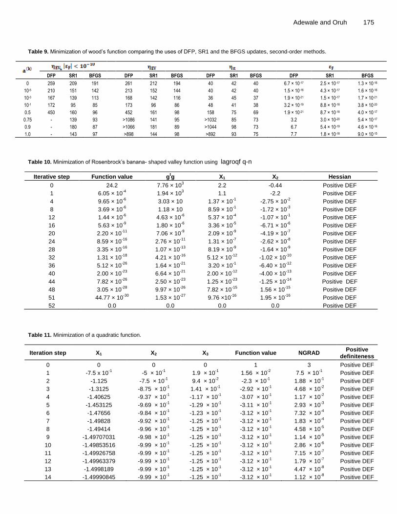
Adewale and Oruh 175 Table 9. Minimization of wood’s function comparing the uses of DFP, SR1 and the BFGS updates, second-order methods.

DFP SR1 BFGS DFP SR1 BFGS DFP SR1 BFGS DFP SR1 BFGS

0 259 209 191 261 212 194 40 42 40 6.7 × 10-17 2.5 × 10-17 1.3 × 10-16

10-5 210 151 142 213 152 144 40 42 40 1.5 × 10-16 4.3 × 10-17 1.6 × 10-16

10-3 167 139 113 168 142 116 36 45 37 1.9 × 10-21 1.5 × 10-17 1.7 × 10-21

10-1 172 95 85 173 96 86 48 41 38 3.2 × 10-19 8.8 × 10-18 3.8 × 10-20

0.5 450 160 96 452 161 98 158 75 69 1.9 × 10-21 8.7 × 10-18 4.0 × 10-17

0.75 - 139 93 >1086 141 95 >1032 85 73 3.2 3.0 × 10-20 5.4 × 10-17

0.9 - 180 87 >1066 181 89 >1044 98 73 6.7 5.4 × 10-19 4.6 × 10-16

1.0 - 143 97 >898 144 98 >892 93 75 7.7 1.8 × 10-18 9.0 × 10-15

Table 10. Minimization of Rosenbrock’s banana- shaped valley function using lagroqf q-n

Iterative step Function value gtg X1 X2 Hessian

0 24.2 7.76 × 103 2.2 -0.44 Positive DEF

1 6.05 × 10-4

1.94 × 103 1.1 -2.2 Positive DEF

4 9.65 × 10-6

3.03 × 10 1.37 × 10-1

-2.75 × 10-2

Positive DEF

8 3.69 × 10-6

1.18 × 10 8.59 × 10-1

-1.72 × 10-3

Positive DEF

12 1.44 × 10-6

4.63 × 10-6

5.37 × 10-4

-1.07 × 10-1

Positive DEF

16 5.63 × 10-9

1.80 × 10-6

3.36 × 10-5

-6.71 × 10-6

Positive DEF

20 2.20 × 10-11

7.06 × 10-9

2.09 × 10-9

-4.19 × 10-7

Positive DEF

24 8.59 × 10-16

2.76 × 10-11

1.31 × 10-7

-2.62 × 10-8

Positive DEF

28 3.35 × 10-16

1.07 × 10-13

8.19 × 10-9

-1.64 × 10-9

Positive DEF

32 1.31 × 10-18

4.21 × 10-16

5.12 × 10-12

-1.02 × 10-10

Positive DEF

36 5.12 × 10-26

1.64 × 10-21

3.20 × 10-1

-6.40 × 10-12

Positive DEF

40 2.00 × 10-23

6.64 × 10-21

2.00 × 10-12

-4.00 × 10-13

Positive DEF

44 7.82 × 10-26

2.50 × 10-23

1.25 × 10-23

-1.25 × 10-14

Positive DEF

48 3.05 × 10-28

9.97 × 10-26

7.82 × 10-15

1.56 × 10-15

Positive DEF

51 44.77 × 10-30

1.53 × 10-27

9.76 ×10-16

1.95 × 10-16

Positive DEF

52 0.0 0.0 0.0 0.0 Positive DEF

Table 11. Minimization of a quadratic function.

Iteration step X1 X2 X3 Function value NGRAD Positive

definiteness

0 0 0 0 1 3 Positive DEF

1 -7.5 x 10-1

-5 × 10-1

1.9 × 10-1

1.56 × 10-2

7.5 × 10-1

Positive DEF

2 -1.125 -7.5 × 10-1

9.4 × 10-2

-2.3 × 10-1

1.88 × 10-1

Positive DEF

3 -1.3125 -8.75 × 10-1

1.41 × 10-1

-2.92 × 10-1

4.68 × 10-2

Positive DEF

4 -1.40625 -9.37 × 10-1

-1.17 × 10-1

-3.07 × 10-1

1.17 × 10-2

Positive DEF

5 -1.453125 -9.69 × 10-1

-1.29 × 10-1

-3.11 × 10-1

2.93 × 10-3

Positive DEF

6 -1.47656 -9.84 × 10-1

-1.23 × 10-1

-3.12 × 10-1

7.32 × 10-4

Positive DEF

7 -1.49828 -9.92 × 10-1

-1.25 × 10-1

-3.12 × 10-1

1.83 × 10-4

Positive DEF

8 -1.49414 -9.96 × 10-1

-1.25 × 10-1

-3.12 × 10-1

4.58 × 10-5

Positive DEF

9 -1.49707031 -9.98 × 10-1

-1.25 × 10-1

-3.12 × 10-1

1.14 × 10-5

Positive DEF

10 -1.49853516 -9.99 × 10-1

-1.25 × 10-1

-3.12 × 10-1

2.86 × 10-6

Positive DEF

11 -1.49926758 -9.99 × 10-1

-1.25 × 10-1

-3.12 × 10-1

7.15 × 10-7

Positive DEF

12 -1.49963379 -9.99 × 10-1

-1.25 × 10-1

-3.12 × 10-1

1.79 × 10-7

Positive DEF

13 -1.4998189 -9.99 × 10-1

-1.25 × 10-1

-3.12 × 10-1

4.47 × 10-8

Positive DEF

14 -1.49990845 -9.99 × 10-1

-1.25 × 10-1

-3.12 × 10-1

1.12 × 10-8

Positive DEF


Table 11. Contd.

15 -1.49995422 -9.99 × 10-1

-1.25 × 10-1

-3.125 × 10-1

2.79 × 10-9

Positive DEF

16 -1.49996567 -9.999 × 10-1

-1.25 × 10-1

-3.125 × 10-1

1.11 × 10-9

Positive DEF

17 -1.499996568 -9.9999 × 10-1

-1.25 × 10-1

-3.125 × 10-1

1.105 × 10-9

Positive DEF

and numerical aspect of quasi-Newton methods that are based on the BFGS formula for the Hessian approximation. We considered only four functions. The performance of BFGS formula make us feel that the superiority of SR1 over BFGS claimed by Khalfan et al. (1993) needed to be probed further, especially, when combined with line searches. Also further study on the use of trust region strategy and line search techniques need to be undertaken. The reader is referred to the work of Nocedal and Yuan (1998). REFERENCES Adewale TA, Aderibigbe FM (2002). A New Line Search Technique,

Quastiones Mathematicae, J. South Afr. Math. Soc. 25(4)453-464. Altman MA (1960). An optimum cubically Convergent Iterative Method

of Inverting a linear bounded operator in Hilbert space. Pacific J. Math. 16:7-113, 1107-1113.

Barnet S (1979). Matrix methods for Engineers and scientists McGraw-Hill Book company New York. pp. 139-145.

Conn AR, Gould NIM, Toint PhL (1988a). Global Convergence of a class of trust region algorithms for optimization with simple bounds. SIAM journal on Numerical Analysis, 25(2):433-460.

Conn AR, Gould NIM, Toint PhL (1988b). Testing a class of methods for solving minimization problems with simple bounds on the variables. Mathematics of computation, 50:399-430.

Conn AR, Gould NIM, Toint PhL (1991). Convergence of quasi-Newton matrices generated by the symmetric rank one update. Mathematical Progamming, 50(2):177-196.

Goldfeldt SM, Quandt RE, Trotter HF (1966). Maximization by quadratic hill-climbing. Econometrica, 34:541-551.

Demidovich BP (1981). Computational Mathematics, MIR publishers, Moscow. pp. 410-490.

Himelblau DM (1972). Applied Nonlinear Programming, McGraw Hill Book Company. New York,pp.30-34, 73-96, 190-217

Khalfan HF, Byrd RH, Schnabel RB (1993). A theoretical and experimental Study of the symmetric rank –one update. SIAM J. Optim. 3(1):1-24.

Levenberg K (1944). A method for the solution of certain problems in least squares. Quarterly Journal on Applied Mathematics , 2:164-168.

Marquardt D (1963). An algorithm for least squares estimation of nonlinear parameters. SIAM Journal on Applied Mathematics, 11:431-441.

Murray W (1972). The Relationship Between The Approximate Hessian Matrices Generated by a Class of quasi – Newton methods, NPL Report NAC 12.

Nocedal J, Yaun T(1998). Combining trust region and line search techniques. Advances in Nonlinear Programming, Kluwer Academic Publishers, Dordrecht, the Netherlands, pp. 153-176,

Pscnichey PS (1978). Numerical Methods in Extremal problems, MIR Publishers, Moscow, pp. 69-129.

Rao CR, Mitra SK (1971). Generalized Inverse of Matrices and its Applications, John Wiley and Sons, New York, pp. 7-9, 207-217.

Rao CR (1973). linear Statistical Inference and its Applications, 2nd

ed. Willey New York pp. 1-50.

Rao SS (1978). Optimization theory and Applications Wily Eastern Limited. New York, pp. 318-720.

Walsh GR (1968). Methods of Optimization, John Willey and Sons, New York. pp. 97-139.

Documents

A theoretical and experimental study of the Broyden