A testing scenario for probabilistic automata

Marielle StoelingaUC Santa Cruz

Frits VaandragerUniversity of Nijmegen

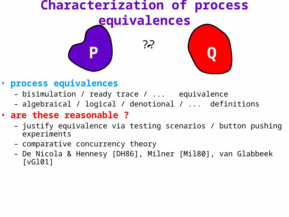
Characterization of process equivalences

• process equivalences – bisimulation / ready trace / ... equivalence– algebraical / logical / denotional / ... definitions

• are these reasonable ?– justify equivalence via testing scenarios / button pushing

experiments– comparative concurrency theory– De Nicola & Hennesy [DH86], Milner [Mil80], van Glabbeek [vGl01]

• testing scenarios:- define intuitive notion of observation, fundamental- processes that cannot be distinguished by observation ce ´: P ´ Q iff Obs(P) = Obs(Q)- ´ does not distinguish too much/too little

P Q´??

Characterization of process equivalences

• process equivalences – bisimulation / ready trace / ... equivalence– algebraical / logical / denotional / ... definitions

• are these reasonable ?– justify equivalence via testing scenarios / button pushing

experiments

• testing scenarios:- define intuitive notion of observation, fundamental- processes that cannot be distinguished by observation are deemed to be equivalent- justify process equivalence ´: P ´ Q iff Obs(P) = Obs(Q)- ´ does not distinguish too much/too little

P Q´??

Main results

• testing scenarios in non-probabilistic case– trace equivalence– bisimulation– ...

• we define – observations of a probabilistic automaton (PA)– observe probabilities through statistical methods (hypothesis testing)

• characterization result– Obs(P) = Obs(Q) iff trd(P) = trd(Q), P, Q finitely branching

• trd(P) extension of traces for PAs. [Segala] • justifies trace distr equivalence in terms of observations

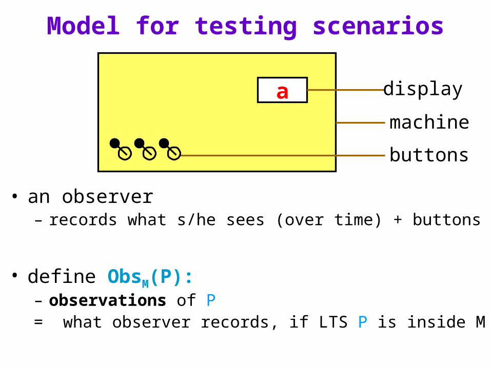
Model for testing scenarios

a

• machine M – a black box– inside: process described by LTS P

• display – showing current action

• buttons – for user interaction

display

machine

buttons

Model for testing scenarios

a

• an observer – records what s/he sees (over time) + buttons

• define ObsM(P): – observations of P= what observer records, if LTS P is inside M

display

machine

buttons

Trace Machine (TM)

a

• no buttons for interaction• display shows current action

Trace Machine (TM)

a

• no buttons for interaction• display shows current action• with P inside M, an observer sees one of , a, ab, ac• ObsTM(P) = traces of P• testing scenario justifies trace (language) equivalence

b c

aP

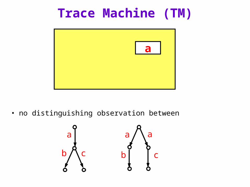
Trace Machine (TM)

a

• no distinguishing observation between

b c

a a a

b c

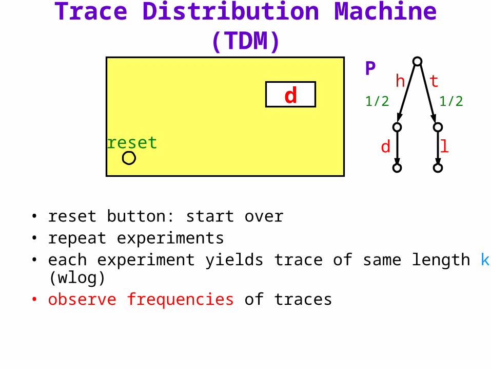
Trace Distribution Machine (TDM)

• reset button: start over• repeat experiments• each experiment yields trace of same length k (wlog)• observe frequencies of traces

d

reset

h t1/2 1/2

d l

P

Trace Distribution Machine (TDM)

• 100 exps, length 2 frequencies - hd tl tl hd tl .... hd hd 48

tl 52

other 0 (hh,dh,hl,...)

d

reset

h t1/2 1/2

d l

P

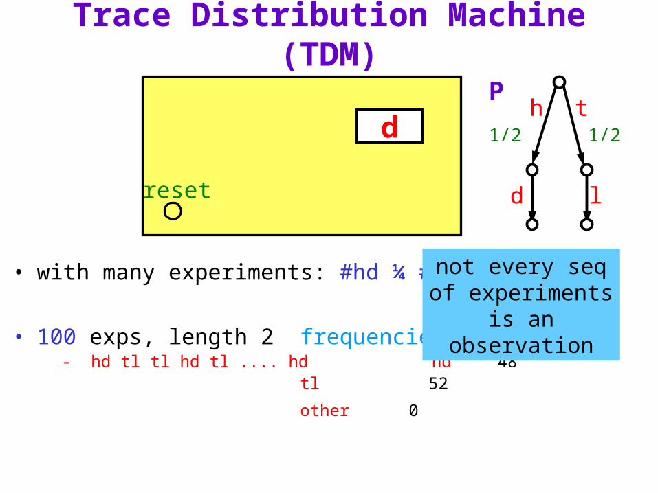
Trace Distribution Machine (TDM)

• with many experiments: #hd ¼ # tl

• 100 exps, length 2 frequencies - hd tl tl hd tl .... hd hd 48

tl 52

other 0

d

reset

h t1/2 1/2

d l

P

not every seq of experiments is an observation

Trace Distribution Machine (TDM)

• with many experiments: #hd ¼ # tl

• 100 exps, length 2 frequencies - hd tl tl hd tl ... hd hd 48

tl 52

other 0 - hd hd hd hd .... hd hd 100 tl 0

other 0

d

reset

h t1/2 1/2

d l

P

2 Obs(P)freq likely

2 Obs(P)freq

unlikely

/

Trace Distribution Machine (TDM)

• nondeterministic choice• choose one transition probabilistically• in large outcomes: 1/2 #c + 1/3 #d ¼ #b• use statistics:

– b,b,b,....b 2 Obs(P) freqs likely

– b,d,c,b,b,b,c,... 2 Obs(P) freqs unlikey

d

reset

b d

1/3 3/4c b

2/3 1/4

P

/

Observations TDM

• ObsTDM(P) = { | is likely to be produced by P}

a

reset

h t1/2 1/2

d l

P

Observations TDM

• perform m experiments (m resets)• each experiment yields trace of length k (wlog)• sequence 2 (Actk)m

• Obs(P) = {2 (Actk)m | is likely to be produced by P, k,m 2

N}• what is likely? use hypothesis testing

a

reset

h t1/2 1/2

d l

P

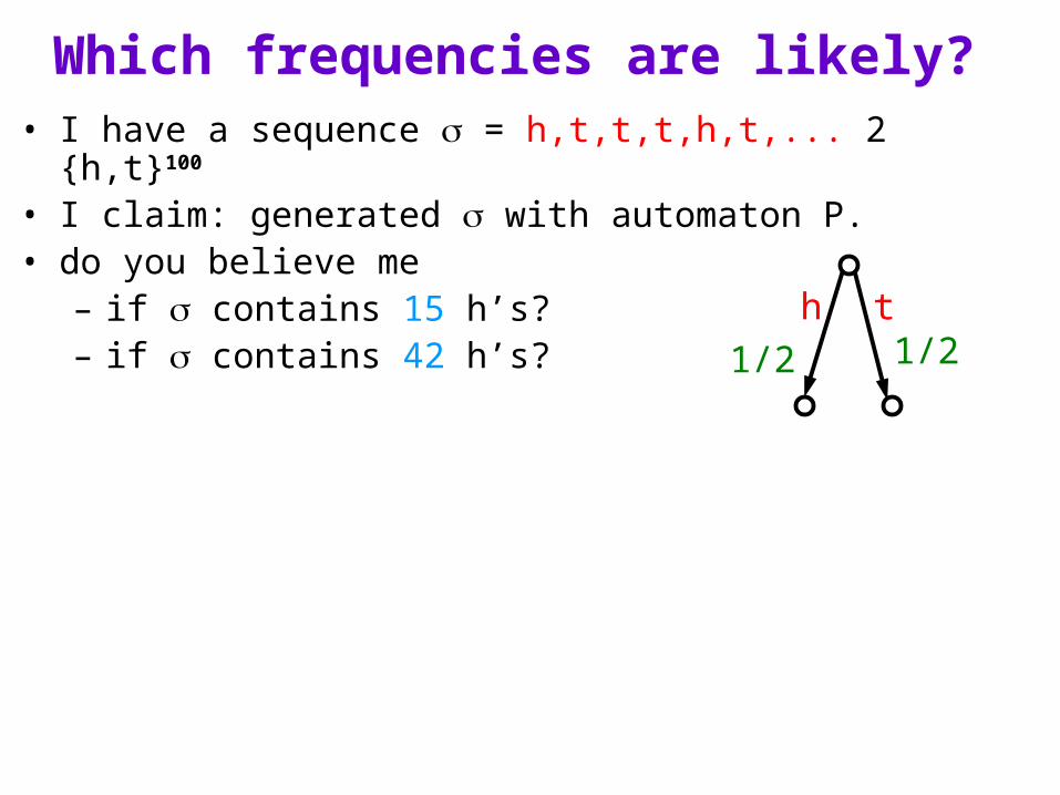
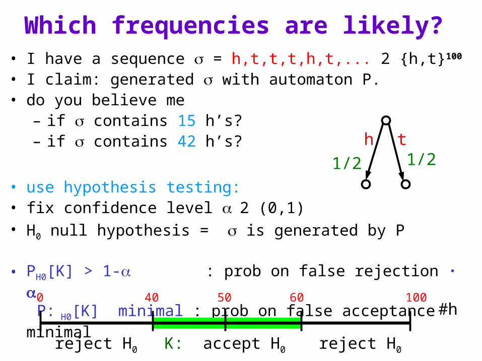
Which frequencies are likely? • I have a sequence = h,t,t,t,h,t,... 2 {h,t}100

• I claim: generated with automaton P.• do you believe me

– if contains 15 h’s? – if contains 42 h’s? h t

1/2 1/2

Which frequencies are likely? • I have a sequence = h,t,t,t,h,t,... 2 {h,t}100

• I claim: generated with automaton P.• do you believe me

– if contains 15 h’s? – if contains 42 h’s?

• use hypothesis testing:• fix confidence level 2 (0,1)• H0 null hypothesis = is generated by P

h t1/2 1/2

0 50 10040 60

K: accept H0reject H0 reject H0

#h

Which frequencies are likely? • I have a sequence = h,t,t,t,h,t,... 2 {h,t}100

• I claim: generated with automaton P.• do you believe me

– if contains 15 h’s? – if contains 42 h’s?

• use hypothesis testing:• fix confidence level 2 (0,1)• H0 null hypothesis = is generated by P

• PH0[K] > 1- : prob on false rejection · P: H0[K] minimal : prob on false acceptance minimal

h t1/2 1/2

0 50 10040 60

K: accept H0reject H0 reject H0

#h

Which frequencies are likely? • I have a sequence = h,t,t,t,h,t,... 2 {h,t}100

• I claim: generated with automaton P.• do you believe me

– if contains 15 h’s? NO – if contains 42 h’s? YES

• use hypothesis testing:• fix confidence level 2 (0,1)• H0 null hypothesis = is generated by P

• PH0[K] > 1- : prob on false rejection · P: H0[K] minimal : prob on false acceptance minimal

h t1/2 1/2

0 50 10040 60

K: accept H0reject H0 reject H0

#h

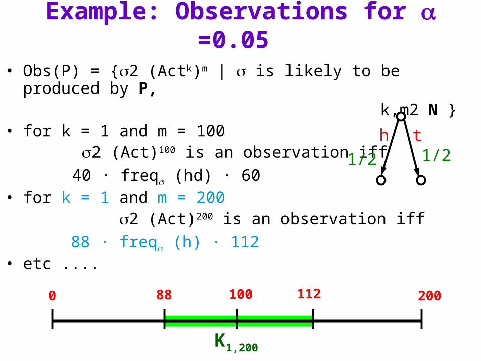
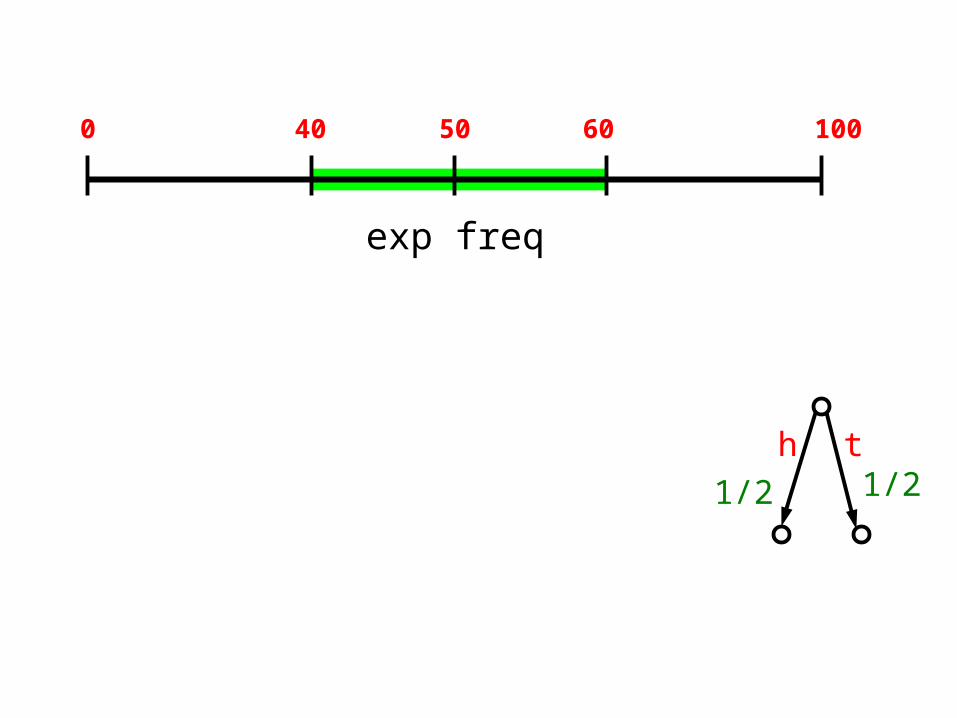
Example: Observations for =0.05

• Obs(P) = {2 (Actk)m | is likely to be produced by P, k,m2 N }• for k = 1 and m = 100 2 (Act)100 is an observation iff 40 · freq (hd) · 60

h t1/2 1/2

0 50 10040

K1,100

60

Example: Observations for =0.05

• Obs(P) = {2 (Actk)m | is likely to be produced by P, k,m2 N }• for k = 1 and m = 100 2 (Act)100 is an observation iff 40 · freq (hd) · 60• for k = 1 and m = 200 2 (Act)200 is an observation iff

88 · freq (h) · 112• etc ....

h t1/2 1/2

0 100 20088

K1,200

112

Example: Observations for =0.05

• Obs(P) = {2 (Actk)m | is likely to be produced by P, k,m2 N }• for k = 1 and m = 100, 2 (Act)100 is an observation iff 40 · freq (hd) · 60• for k = 1 and m = 200 2 (Act)200 is an observation iff

88 · freq (h) · 112• etc ....

h t1/2 1/2

0 100 20088

K1,200

112

exp freq EP

allowed deviation ( = 12)0

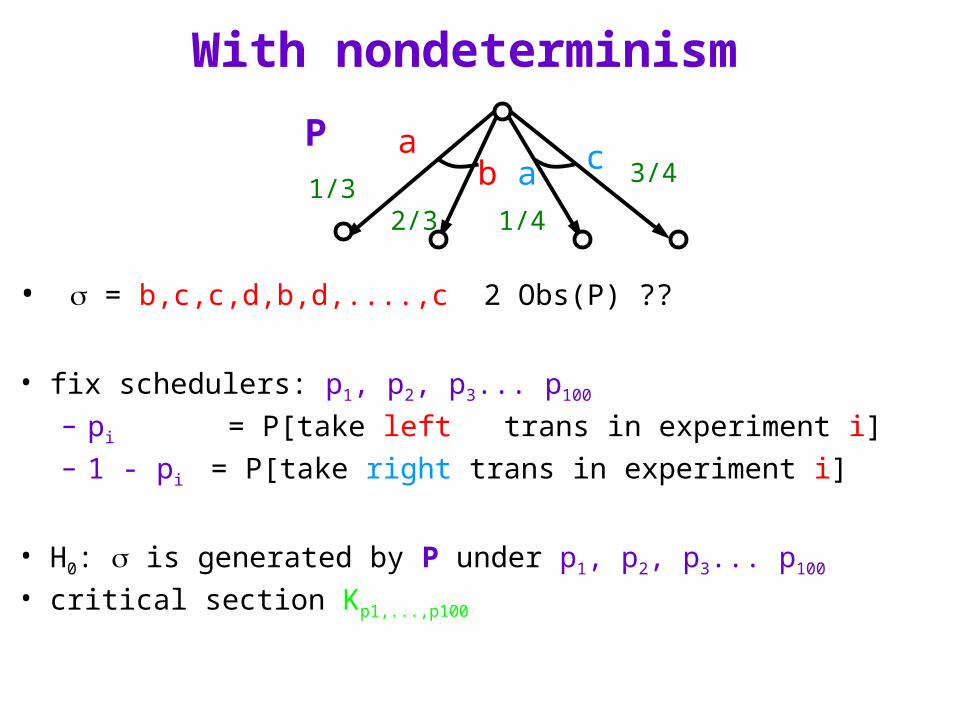
With nondeterminism

• = b,c,c,d,b,d,....,c 2 Obs(P) ??

aa1/3

3/4b c

1/42/3

P

With nondeterminism

• = b,c,c,d,b,d,....,c 2 Obs(P) ??

• fix schedulers: p1, p2, p3... p100

– pi = P[take left trans in experiment i] – 1 - pi = P[take right trans in experiment i]

• H0: is generated by P under p1, p2, p3... p100 • critical section Kp1,...,p100

aa1/3

3/4b c

1/42/3

P

With nondeterminism

• = b,c,c,d,b,d,....,c 2 Obs(P) ??

• fix schedulers: p1, p2, p3... p100

– pi = P[take left trans in experiment i] – 1 - pi = P[take right trans in experiment i]

• H0: is generated by P under p1, p2, p3... p100 • critical section Kp1,...,p100

aa1/3

3/4b c

1/42/3

P

2 Obs(P) iff 2 Kp1,...,p100 for some p1, p2, p3... p100

Example: Observations

Observations for k =1, m = 100. • contains b,c only with 54 · freq (c) · 78

– take pi = 1 for all i• contains b,d only with 62 · freq (d) · 88

– take pi = 0 for all i

bb1/3 3/4c d

1/42/3

Example: Observations

Observations for k =1, m = 100. • contains a,b only and 54 · freq (c) · 78

– take pi = 1 for all i• contains b,d only and 62 · freq (d) · 88

– take pi = 0 for all i

Observations for k=1, m = 200 • 61 · freq (c) · 71 and 70 · freq (d) · 80

– pi = ½ for all i (exp 66 c’s; 74 d’s; 60 b’s) – (these are not all observations; they form a sphere)

bb1/3 3/4c d

1/42/3

Main result

• TDM characterizes trace distr equivalence

ObsTDM(P) = ObsTDM(Q) iff trd(P) = trd(Q)

if P, Q are finitely branching

• justifies trace distribution equivalence in an observational way

Main resultTDM characterizes trace distr equiv ´TD

ObsTDM(P) = ObsTDM(Q) iff trd(P) = trd(Q)

• “only if” part is immediate, “if”-part is hard.– find a distinguishing observation if P, Q have different trace distributions.

• IAP for P. Q fin branching – P, Q have the same infinite trace distrs iff P, Q have the same finite trace distrs

• the set of trace distrs is a polyhedron• Law of large numbers

– for random vars with different distributions

Observations =0.05

• Obs(P) = {2 (Actk)m | likely to be produced by P}

• Obs(P) = {2 (Actk)m | freq_ in K} •

• for k = 1 and m = 100, 2 (Act)100 is an observation iff 40 · freq (hd) · 60

h t1/2 1/2

0 50 10040 60

K

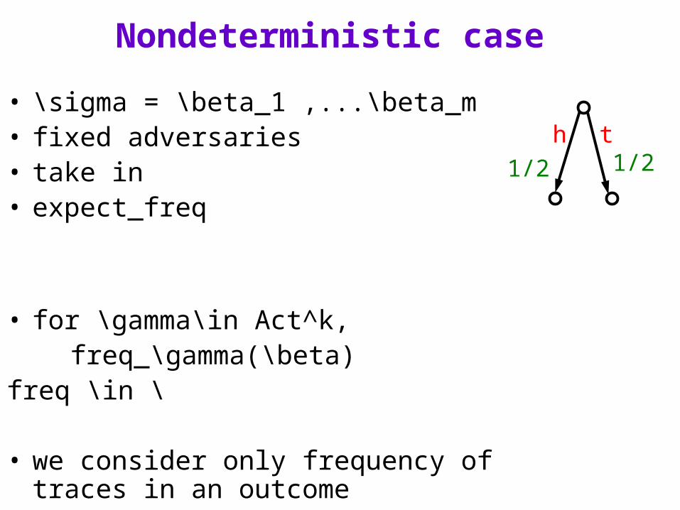
Nondeterministic case

• \sigma = \beta_1 ,...\beta_m• fixed adversaries• take in • expect_freq

• for \gamma\in Act^k, freq_\gamma(\beta) freq \in \

• we consider only frequency of traces in an outcome

h t1/2 1/2

a!

b!

a?

b?

b c

a

a!

b!

a?

Trace Distribution Machine (TDM)

• reset button: start over• repeat experiments: yields sequence of traces• in large outcomes: #hd ¼ # tl• use statistics:

– hd,hd,hd,...,hd 2 Obs(P) too unlikely – hd,tl,tl,hd,...tl,hd 2 Obs(P) likely

d

reset

/

h t1/2 1/2

d l

h t1/2 1/2

0 50 10040 60

exp freq

Process equivalences

Q

P

Testing scenario’s

a

• a black box with display and buttons• inside: process described by LTS P• display: current action• what do we see (over time)? ObsM(P)• P, Q are deemed equivalent iff ObsM(Q) = ObsM(Q)• desired characterization:

display

machine

buttons

Observations =0.05

• Obs(P) = {2 (Actk)m | is likely to be produced by P}• for k = 1 and m = 99,• expectation E = (33,33,33) • Obs(P) = {2 (Act)99 | | – E | <

15}

h t1/3 1/3