A Test of the Validity of Steady State and Equilibrium Approximations in Chemical Kinetics Vincente Viossat and Roger I. Ben-Aim Universite P. et M. Curie - 75005 Paris (France)

Kinetic studies focus on various interests, including physical parameters (temperature, initial concentrations, etc.) and kinetic data (orders, activation energies, etc.). Such studies in closed and homogeneous systems a t cou- stant volume and temperature generally lead to nonlinear ordinary differential equations: the chemical rate equa- tions. These equations have the following form.

where the concentrations of the species are denoted as XI, ..., x"; and the corresponding time derivatives are denoted by x,, ...,i,,.

In general these differential systems are difficult to solve analytically, so approximate or numerical solutions are often used. A general method for obtaining such appmxi- mate solutions is to suppose that some of the functions f,, ..., fi are equal to zem. The system thus becomes

f1 = 0

This system of j algebraic equations and n - j differential equations clearly has a simpler solution than the initial system.

This method is similar to the theom of dvnamical svs- tems where information about the system is obtained from stationarv solutions of all the variables. These stationarv solutionsdefine the "attractor" that the system approaches when the time tends to i n f i t y .

Evidently, relations such as f i = 0 and fi = 0 allow expres- sion o f j concentrations as functions of the other n - j con- centrations that are time-dependent. This is why the X I , ..., x, concentrations, which are now implicit functions of time, are called "quasi-stationary". Solving the remaining n - j differential equations leads to a solution that is an appmx- imation of the initial system.

In this paper we investigate the following very simple mechanism, from this point of view.

1 3

A ~ B - c

2

where A is the reactant; B is the intermediate compound; and the Cis product.

732 Journal of Chemical Education

This mechanism is often encountered in chemical kinet- ics. Some examples are well-known:

a acid-base catalysis ( I ) enzyme catalysis (2) transition-state theory (3) quasi-unimolecular reaction theory by Lindemann (41 nucleophilic and electrophilic substitutions (5)

Two bfferent cases corresponding to the general method of approximation described above will be considered:

Quasi-Stationary State Approximation (QSSA) r Quasi-Equilibrium Approximation (QEA)

The exact solution for this mechanism is obtained when the reactions are first-order. Afterwards, the analytical ex- pressions of the solutions calculated using the above ap- ~mximations are derived. Finallv the solutions are com- pared either analytically or by"numerica1 simulations. Thus, the conditions of validity of the a~~roximations verv commonly used in chemistry are pi t ' in evidence an; tested.

Kinetic Equations and Analytical Solutions Exact Theory

The rates of reactions 1, 2, and 3 are denoted by u,, u,, and US. The concentrations of A, B, and C are denoted by the same symbol as the corresponding chemical species. The elementary reaction rates are assumed to be first- order.

The overall rate is calculated either for the reactant de- let ion

"=-A=" 1 - 0 2

or for the accumulation of final

U ' = C = ~ 3

Generally the rates u and u' are different due to the pres- ence of the intermediate compound B.

The kinetic equations are

A = -vl+ uz =-k,A+ k,B (11

B = V ~ - U ~ - U ~ = ~ , A - ~ , B - ~ ~ B system 1 (2)

C=u3=kSB (3)

System 1 clearly corresponds to a particular case of the general mechanism reported in the introduction.

I t is customary to consider the following initial condi- tions.

A(O) = %

B(0) = C(0) = 0

The solution of system 1 has been given by Lowry and John (63, Johnson (71, Rodiguin and Rodiguina (8).

A - = (b - A,)-'(& - kl) et'~t) - (XI - kl) et"lt) 4

with

With conditions ii, the solution is

Quasi-Stationary State Approximation

In the QSSA(9) one assumes

u l - " ~ - U 3 = 0 (2') C = (kz + k,) k l + k , + k 3 " [I - AE])

(9') Equation 2' replaces eq 2 in the differential system 1. It follows that the overall reaction rates u and u' calculated for the reactant or the product are the same. The differen- tial system is

A = - k , ~ + k @ (1)

We may notice that eqs 7',8', and 9' are deduced from eqs 7,8, and 9 by changing & into

system 2 (2') As noted previously, it is evident that eq 8 does not sat-

isfy the condition B = 0 at t = 0. For this reason QSSA is applied only during a certain time interval &er the reac- tion begins, as usually specified in textbooks. The solution of system 2 depends on integration con-

stants, which in turn are specified by the initial time. How- ever, the exact initial conditions,

A(0) = %

Quasi-Equilibrium Approximation

In the QEA (10) one assumes

v , -v ,=o (1')

Equation 1' replaces eq 1 in the differential system 1, which becomes

0=-klA+k2B ( 1')

B = klA - (k, + k,)B system 3 (2)

do not hold for eq 2'. It is absolutely necessary to adopt initial wnditions consistent with eq 2'. which wnstitutes the basis of the approximation. Two simple different condi- tions come to mind:

-i: A(0) = % =$

The overall reaction rate u for reactant depletion is al- ways null, whereas u', the reaction rate for product accu- mulation, is nontrivial and always positive (except at the beginning and the end of the reaction). This surprising re- sult wmes from the hypothesis that, at each time, the equi- librium between A and B is reached while B reads to form C.

Solution of system 3 evidently depends on integration constants. At the initial time, the exact initial conditions

4 0 ) = %

and

C(0) = 0

(At t = 0 the concentrations of A and C are the exact ones, whereas the concentration of B is modified. As a result, the mass balance of the whole system is not obeyed.)

do not hold for eq 1'. We decide to maintain eq 1' and one of the following conditions:

(Mass is conserved but the initial conditions are modified for Aand B.)

Acwrding to the wnditions adopted, it is easy to obtain the integrated form of system 2.

With conditions i, the solution is and

C(0) = 0

(Mass is not conserved at t = 0, and the initial condition for B is modified.)

Volume 70 Number 9 September 1993 733

8 the differential system 1 (A+ B + c = 0 ) 8 the integrated expressions of A, B, and C

or 8 simple chemical considerations

The parameter r = A + B + C is introduced for approximate solutions, and the ratio rl& is compared to 1.

and

Quasi-Stationary State Approximation

With QSSA and initial conditions i, (Mass is conserved, but the initial conditions are modified for A and B.)

According to the condition adopted, it is easy to obtain the integrated form of system 3. With conditions i, the so- lution is

The limited expansion for a short time interval is

The condillon that makes this expression close to 1 for the initial time and fir the shon time intervals is k l << k. r k ~ .

From eqs 7 and 9, it is easy to obtain t , and T, half-lives associated with system 2:

With conditions ii, the solution is

Evidently these two values are different from the exact half-lives, tvz and Tm, obtained with the system 1. Substi- tuting t with t,, eq 13 becomes

A less-restrictive condition is obtained for mass conserva- tion at half-lives

k , << 2(kz + k3)

For long time intervals the exponential term ofeq 13 tends to zero, and the law is always obeyed.

With QSSA and initial conditions ii

Note that eqs 10', ll', and 12' are deduced from eqs 10,11, and 12 by changing & into

Criterion for Testing the Validity of Approximations In general, for any problem solved in an approximate

manner, it is necessary to check the validity of the approx- imation. In this particular problem one criterion has been chosen: the mass conservation law. Comparison between

This expression is deduced from 13 by changing A, into

the exact and approximate solutions is c&ed out by ana- lytical or numerical methods or both.

The test will he applied at dlmerent time intewuls during the course of the reaction:

0 short time intervals half-lives (tvz for reactant consumption; Tm for product formation) long time intervals

In the previous calculations, solutions have been ob- tained by assuming that the approximation is valid a t the initial time and consequently changing the initial condi- tions for B or Aor both. In both cases i, the mass consenra- tion law is not obeyed. Thus, this statement cannot be maintained from a chemical point of view except as an ap- proximation.

The mass conservation law is evidently

v t : A + B + C = %

and the approximation is applicable. As a conclusion, the condition k l << kz + k3 , with consis-

tent initial concentrations, makes QSSA valid from the point of view of mass law conservation.

Quasi-Equilibrium Approximation

With QEAand initial conditions i,

and follows from

734 Journal of Chemical Education

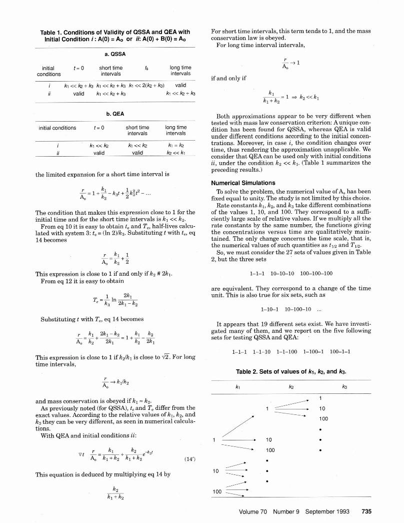
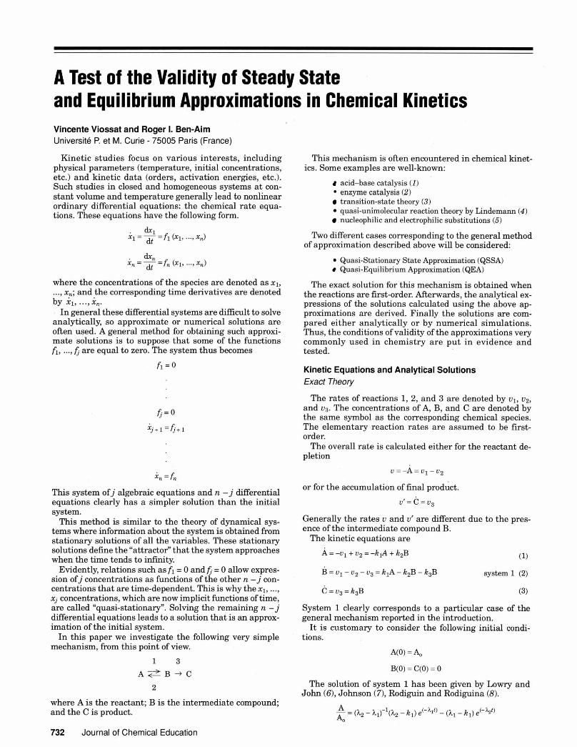
Table 1. Conditions of Validity of QSSA and QEA with Initial Condition i : A(0) = A. or ii: A(0) + B(0) = Ao

a. QSSA

initial t = O shorttime t long time conditions intervals intervals

i ki << k2 + k3 ki << k2 + k3 k~ << Z(k2 + k3) valid ii valid ki << k2 + k ki<<k2+k

b. QEA

initial conditions t = O shorl time long time intervals intervals

i kr c< k2 ki <c k2 kl = k ii valid valid k2 << kl

the limited expansion for a short time interval is

The condition that makes tlus expression close to 1 for the initial time and for the short time intervals is k, <c k l .

From eq 10 it is easy to obtain t . and T,, half-lives calcu- lated with system 3: t . = (In 2)lkg. Substituting t with t,, eq 14 becomes

This expression is close to 1 if and only i f k z # 2k. From eq 12 it is easy to obtain

Substituting t with T,, eq 14 becomes

This expression is close to 1 if kzlkl is close to a. For long time intervals,

and mass conservation is obeyed if kl = kz. As previously noted (for QSSA), t , and T. differ from the

exact values. According to the relative values of kl , kz, and ka they can be very different, as seen in numerical calcula- tions.

With QEA and initial wnditions ii:

This equation is deduced by multiplying eq 14 by

For short time intervals, this term tends to 1, and the mass conservation law is obeyed.

For long time interval intervals,

if and only if

Both approximations appear to be very different when tested with mass law conservation criterion: Aunique con- dition has been found for QSSA, whereas QEA is valid under different conditions according to the initial concen- trations. Moreover. in case i. the condition chanees over ~ ~

time, thus rendering the ap6oximation unapphcible. We consider that QEAcan be used onlv with Initial conditions ii, under the condition kz << k l . ('fable 1 summarizes the preceding results.)

Numerical Simulations To solve the problem, the numerical value of A,, has been

fixed equal to unity The study is not limited by this choice. Rate wnstants k l , kz, and k3 take different combinations

of the values 1, 10, and 100. They correspond to a suffi- ciently large scale of relative values. If we multiply all the rate constants by the same number, the functions giving the concentrations versus time are qualitatively main- tained. The only change concerns the time scale, that is, the numerical values of such quantities as tn and Tm.

So, we must consider the 27 sets of values given in Table 2 , but the three sets

are equivalent. They correspond to a change of the time unit. This is also true for six sets, such as

It appears that 19 different sets exist. We have investi- gated many of them, and we report on the five following sets for testing QSSAand QEA:

Table 2. Sets of values of ki, h, and k3.

Volume 70 Number 9 September 1993 735

Geometrical Representation Let us represent A, B, and C, as

the coordinates along three per- pendicular axes. Mass conserva- tion gives

A + B + C = %

which is the equation of a plane called the "simplex" of the sys- tem.

Every trajectory that satisfies the mass conservation is in- cluded in this plane, as is the exact solution of system 1. The

a s e b simplex intercepts the axes at three points (a, b, and c) defining an equilateral triangle of side equal to a&. It is well-estab- lished in phase diagrams (Fig. l a ) that a point M inside the =h *

equilateral triangle can repre- sent the composition of a ternary system: The distance to the side bc is proportional to the concen- tration A, and so on.

Ao The sum of the distances to the

three sides is a constant equal to the altitude h of the triangle. Be- cause the side is equal to &*, h

0 e e' i s&m The composition of the system

can be followed either in the tri- ~ ~

Figure 1. (la) Spatial representation of the system of three constituents A. 8, and C. Every system dimensional space or, more con- satisfying mass conservation is represented in the "simplex" plane abc. (1 b) Exact trajectory of the venientl~, in the The system in the "simplex". (Ic) Approximate trajectories corresponding to QSSA with initial wnditbns ior exad trsjectoly starts at point a ii. (Id) Approximate trajectories corresponding to QEA with initial conditions ior ii. and ends at point c (Fig. lb).

QSSA and QEA stipulate, re-

Miller (15) points out that simplified equations differ with QSSA according to whether or not the mass law is conserved. References 16, 10, and 17 also compare QSSA and QEA. The former gives the integrated form of the equations with the steady state approximation and initial and conditions i. The condition k l << kz + k3 makes the exact and approximate expressions of A, B, and C identical. For QEA the author states the condition klA = k.B and uses

spectively, the relations

mass conservation. The only kinetic law conc&ns product (eq 3), He obtains certain conditions that make identical which are the equations of two different planes including

QSSA and QEA. the axis OC and intercepting the simplex along straight lines cs and ce, respectively (Fig. la).

Reference 10 considers both approximations and com- nares The initial conditions i applied to QSSAare

the exact expression for the rate equation for C with the ap- proximate rate obtained from the use of the ... approximation

A s the authors limit the study to differential equations, the problem of initial conditions does not appear. The study is also limited by the fact that they consider only the cases corresponding to k l = kz or k l = k ~ , as seen in Figures 3 and 4 of their paper.

The conclusion is that QSSA is valid if k3 >> kz or if k3 << k z with the condition kl = kz or k l = k3 , respectively. It is in agreement with our condition k l << kz + k,. The conclusion that QEAis valid if k 1 = ks << kz does not have an exact equivalent in our study. However,it corresponds to our initial conditions r for short time intervals (compare with Table lb). The authors reiecc the condition k l = k. >> - . k3, though it appears in plots i f Figure 4 of their paper.

Sehmitz (1 7) presents many theoretical mechanisms and compares QSSA and QEA. However, a clear conclusion does not appear.

C(0) = 0

The initial conditions i applied to QEAare

A(0) = 4

They are the coordinates of points s' and e', respectively. The initial conditions ii are, for QSSA,

Volume 70 Number 9 September 1993 737

C(0) = 0

For QEA,

They are the wordinates of points s and e because they satisfy the following relation.

A(0) + B(0) = 4

Description of the trajectories during the progress of the readion is an interesting subject, but it is outside the swpe of this paper. The exact trajectory is contained in the sim- plex plane abc (Fig. lb). The trajectories corresponding to QSSA or QEA are contained in planes cOs or cOe, respec- tively, as shown in Figures l c and id.

If, as usually but inwnsistently admitted, the exact ini- tial conditions are adopted and QSSAis applied, the trajec- tory stark at point a and tends to the plane cOs. The time necessary to approach this plane corresponds to the "in- duction period" during which the steady state cannot be applied.

On the contrary if, according to our view, QSSA is ap- plied from the beginning of the reaction, the trajectory is located entirely in the plane cOs. For example, with wndi- tion ii, it stark a t points and ends a t point c. The more the mass conservation law is obeyed, the more the trajectory goes nearer the simplex, that is, the straight line sc. The condition of validity of QSSA, kl << k;? + ka makes s and s' draw nearer to a , and the three trajectories, ac, sc, and s'c are merging. I t is evident that the concentration of B be- comes very small. It is noteworthy that, as QSSAis always valid for long time intervals, the trajectories are tangent to the straight line sc when they approach c.

Concluding Remarks - In this paver QSSA and QEA have been applied to a par-

ticular m&anis& of importance in chemic~kinetics.The approximate solutions were calculated with initial wndi- tiois consistent with the approximations.

The validity of approximations was tested with the crite- rion of mass balance. Other criteria could have been cho- sen, such as comparison between

approximate and exad concentrations Cap#& reaction rates u,#~.. characteristic times tapdt,, concentration of intermediate Bap&

I t would be interesting to check the results obtained in these different cases.

The advantage of the criterion chosen is that it does not need inteeration of the set of exact eauations because mass balance & generally obtained from chemical considera- tions, whereas some of other criteria need this integration. Thus, our method can be applied in more complex systems. The results obtained are the following.

QSSA, applied with initial coherent conditions, is valid from the very heginning and d m g the progress of the reaction under rhe condition k . << ko + k,. Thiscondition is in wee- ment with many publhed;esuks.

QEAcannot be applied without caution. Different conditions appear awarding to the example chosen. The only case in which coherence is achieved all along the reaction progress corresprmds to the condition kl >> kz with initial conditions ii. Howwer, the problem of compatibility of these mnditions with the results published so far has not been investigated.

Acknowledgment

The authors thank G. Nicolis of Bruxelles University for critical reading of the mannscript.

Literature Cited 1. Ben, R. PAcX M d h C a h l ~ i s ; Clarendan: (Mmd. 1941; p9O. 2. Michaelis, L.;Menten, M. L.Bioekk 2. 1913,49,333. 3. E-, H. J A m Chem Soc. 1891,53,ZS31; or C h . Phys. 19%2,10, 103. 4. Liodemm, F. A. Ihuls. Fomduy Sae. 188% 17,598.

5. Ingold, C. K Sfrubun end Medonism in I~lg~lgnie Chamiaw, 2nd ed.: Cornell Univemity: Ithaca. NY. 1969.

6. Lomy, T. M.; John, W. T J. Chem. Sae. 1910,97,2634. 1. Jahoaon, K J. Numriml M&& in Chemistry; Marcel Dekker: NewYork aod

Base1 Radri-, N.M.;Rodri-a.E N. C o ~ e c v t i ~ ChemrmlR-tlolo,Vao Noehaod:

lbronto, NewYork London, 1961. . Bod-tein, M. Z Physikalkhr Chem. 1013,85,341.

10. Valk, L.: R i c h a r b , W.; La", K H.; Lin, S. H. J. Cham. Edue. 1817,64,95. 11. Gilbert,H. F J. Chem.Edue. 1677,64,492. 12. Rain-. R T.: Ransen. D. E. J Chem. Edw. 19E% 65.161. . . . . 13. Porter. M. D., Skinner, G. B. J Chem Edue. IWS,53,366. 14. Tardy, D. C.; Cater, E. D. J Ckm. Ed=. ISSS, 60,109. 15. Miller, S. 1. J. Chem Ed=. 18811.62.490. 16. Pyuo, C. W J Chem. Educ. 1071,48. 194.

17. Sehmitz. G., Thesis, IVniversitd libre de BmeUe~es, Stationnarite et rkt ions pC&ques, 1983.

738 Journal of Chemical Education