A Test of Private Information in Life Insurance Markets

NBER WORKING PAPER SERIES

MULTIPLE DIMENSIONS OF PRIVATE INFORMATION IN LIFE INSURANCEMARKETS

Xi WuLi Gan

Working Paper 19629http://www.nber.org/papers/w19629

NATIONAL BUREAU OF ECONOMIC RESEARCH1050 Massachusetts Avenue

Cambridge, MA 02138November 2013

Authors would like to thank seminar participants at Columbia University, University of California,Davis and Miami University for their help comments. All the remaining errors are ours. The viewsexpressed herein are those of the authors and do not necessarily reflect the views of the National Bureauof Economic Research.

NBER working papers are circulated for discussion and comment purposes. They have not been peer-reviewed or been subject to the review by the NBER Board of Directors that accompanies officialNBER publications.

© 2013 by Xi Wu and Li Gan. All rights reserved. Short sections of text, not to exceed two paragraphs,may be quoted without explicit permission provided that full credit, including © notice, is given tothe source.

Multiple Dimensions of Private Information in Life Insurance MarketsXi Wu and Li GanNBER Working Paper No. 19629November 2013JEL No. D82,G22,I13

ABSTRACT

Conventional theory for private information of adverse selection predicts a positive correlation betweeninsurance coverage and ex post risk. This paper shows the opposite in the life insurance market despitethe clear evidence of private information on mortality risk. The reason for this contradictory resultis the existence of multiple dimensions of private information. The paper discusses how the privateinformation on insurance preference offsets the effect of the private information on mortality risk.A mixture density model is applied to disentangle these two effects.

Xi WuDepartment of EconomicsTexas A&M UniversityCollege Station, TX [email protected]

Li GanDepartment of EconomicsTexas A&M UniversityCollege Station, TX 77843-4228and [email protected]

2

I. Introduction

Much literature has argued that adverse selection or moral hazard induced by the

private information may lead to an under-provision or lack of trade in insurance,

causing a substantial consumer welfare loss. However, this paper shows that people

who have lower mortality risk are more likely to have life insurance, despite the clear

evidence of private information on mortality risk. The reason for this contradictory

result is the existence of multiple dimensions of private information. The paper

discusses how the private information on insurance preference offsets the effect of the

private information on mortality risk and applies a mixture density model to

disentangle these two effects.

As one of the most widely held financial products, by the end of 2009, total life

insurance coverage in the United States had achieved $18.1 trillion (American Council

of Life Insurance, 2010). In light of its large size, it is important to understand the

influence of the private information in this market.

Rothschild and Stiglitz (1976) argue that individuals may still have residual

information about their own eventual risk in a competitive market after conditional on

all observables to insurers. Those who believe they have higher risk would purchase

more insurance than those lower-risk individuals. Therefore, one standard test for

detecting asymmetric information used in most literature is to test for a positive

correlation between the amount of insurance coverage and ex post occurrence of

insured risk (Chiappori and Salanié 1997, 2000; Chiappori, Julian, Salanié, and

Salanié, 2006).

Existing empirical literature on asymmetric information in life insurance markets,

however, is mixed. Cawley and Philipson (1999) found a neutral or even negative

relationship between life insurance ownership and subsequent mortality using 1992-

1994 Health and Retirement Study (HRS) data. We find similar results using HRS data

during the period between 2000 and 2008. In Table 1, 20.6% of people in the sample

passed away during the period of 2000 and 2008. However, the mortality rates are

quite different by life insurance. Among 69.5% of people who have life insurance in

year 2000, 18.4% of them passed away. Meanwhile, 25.6% of people who do not have

life insurance died.

3

Various explanations for this interesting phenomenon are offered in the literature.

Pauly et al (2003) explain the absence of private information with individuals’

sufficiently low risk elasticity. They argue that even if individuals indeed know more

than insurers, serious adverse selection will not occur if those individuals are sluggish

in their willingness to respond to that information. He (2009), however, attributes the

absence to a sample selection problem: Even if high-risk individuals are more likely to

purchase life insurance, they are also more likely to die early and thus less likely to be

found in a cross-sectional sample.

Recent theoretical research suggests that a positive correlation between insurance

purchases and risk occurrence is neither necessary nor sufficient for the presence of

asymmetric information about risk type when multiple dimensions of private

information, such as risk type or insurance preferences, coexist (Smart, 2000; De

Meza and Webb, 2001; Jullien, Salanié, and Salanié , 2007; Chiappori and Salanié,

2013). To illustrate, consider the following thought experiment. There are five

individuals each in groups I and II, which are a high-insurance-preference (h) group

and low-insurance-preference (l) group, respectively. The l group is more likely to die

and has a weaker preferences in insurance; while, the h group has a lower probability

to experience the risky event but has a stronger preferences for insurance. As shown in

Table 2, the probability to die for individuals 1 to 5 in group I is 20, 30, 40, 50, and 60

percent, respectively; and the corresponding amount of insurance purchases for this

group is 1, 1, 2, 3, and 4. For individuals A to E in group II, their mortality risks are 10,

20, 30, 40, and 50, respectively; and the amount of insurance purchased by this group

is 1, 2, 2, 3, and 4. If we combine these two groups as a whole, a researcher examining

this sample may conclude that the asymmetric information is absent: When the

probability of mortality is increased from 50 to 60 percent, the amount of insurance

purchased, on the contrary, decreases from 7 to 4. However, a positive correlation

between individual insurance purchases and the probability of ex post risk can be

found, conditional on each category of individuals’ insurance preferences.

Empirically, Finkelstein and McGarry (2006) demonstrate the existence of these

multiple dimensions of private information on risk type and on individual insurance

preferences in long-term care insurance markets. They confirm that these two

4

dimensions of private information operate in offsetting directions, leading to a neutral

or negative relationship between insurance coverage and the occurrence of risky events,

even if the market is known to have asymmetric information on ex post risk. However,

despite direct evidence of private information on risk type, they still fail to detect it

using the “positive correlation” test by controlling proxy variables for individuals’

preferences in insurance.

Intuitively, when a full set of proxy variables for insurance preferences is available,

controlling these variables enables us to fully exclude the effect of heterogeneous

insurance preferences on the relationship between insurance purchase and subsequent

mortality. However, under most circumstances, the accessibility of only a partial set of

proxy variables related to insurance preferences would lead to the error term still

consisting of these two kinds of private information, resulting in failures of the

standard test for private information. (See Gan, Huang, and Mayer (2011) for a more

formal discussion on this point.)

This paper makes three contributions to the literature. First, contrary to the

conclusions drawn in Cawley and Philipson (1999), this paper provides direct evidence

of private information in life insurance markets. In particular, after conditioning on a

set of variables used by insurance companies for the determination of risk

classifications, individuals’ subjective responses on their own mortality risks that are

available in HRS (but not typically available to insurance companies) have additional

predictive power to their actual mortality risks. Nevertheless, the traditional positive

correlation test fails to detect this asymmetric information.

Second, we find a series of socioeconomic factors, which are correlated with the

second type of private information (i.e., heterogeneity in insurance preferences), and

show that this type of private information has an opposite effect on insurance purchase

and subsequent mortality. Similar results are reported by Finkelstein and McGarry

(2006) and Cutler, Finkelstein, and McGarry (2008). Specifically, individuals who

have stock, houses, and loans, as well as those who have employment are more likely to

buy life insurance but less likely to experience insured event. Similarly pattern applies

to individuals who have more years of education, more annual income, lower risk

tolerance and stronger bequest motives. However, with the effort of excluding

5

individuals’ heterogeneity in insurance preferences through controlling these variables,

we still fail to find a positive correlation between life insurance purchases and

subsequent mortality.

Third, this paper applies the mixture density model, in which we separate

individuals into two unobserved types based on their different preferences in life

insurance. Under this framework, we successfully obtain a significant and positive

correlation between life insurance purchases and subsequent mortality conditional on

each type. It is worth pointing out that, due to the specificity of life insurance markets,

a positive correlation between life insurance ownership and subsequent mortality

signifies the existence of adverse selection, in light of the small possibility of moral

hazard in this market. Our result also implies that, different from long-term care

insurance markets shown by Finkelstein and McGarry (2006), such heterogeneity in

preferences of life insurance is driven by a variety of socioeconomic factors, not solely

the risk attitude.

The remainder of this paper proceeds as followings. In section II, we illustrate the

identification strategy used to detect the private information in life insurance market

and describe our data. Section III presents the results and specification test. The final

section concludes.

II. Empirical Approach

Our empirical strategy proceeds in three steps. First, we demonstrate that

individuals have residual private information about their mortality risk; and this

residual information is also negatively correlated with insurance coverage. However,

the standard positive correlation test does not provide any evidence for the existence of

this private information. Second, we empirically identify a set of socioeconomic factors

which are related to the second type of private information, (i.e., the heterogeneity in

insurance preferences) and show that they can offset the effect of the private

information on mortality risk on the correlation between insurance coverage and risk

exposure in life insurance markets. In the final step of our analysis, we apply the

mixture density model and present that a positive correlation between insurance

coverage and insured event can be obtained only if individuals’ insurance preferences

6

is conditioned by distinguishing people into two groups based on the series of factors

we mentioned above.

A. Econometric Model

We characterize the market for life insurance with the following two equations.

The first equation relates the individual characteristics to the probability of mortality.

The second relates the same characteristics to the decision to purchase life insurance.

1( 0)

1( 0)

X H SS

X H SS

Die c X H SS u

LFI c X H SS v

, (1)

where Die is an indicator variable for whether the individual died during the period

2000-2008. LFI is a binary variable for whether the individual had life insurance in

year 2000. We chose year 2000 as the starting period because the 2000 wave is the

first year that includes all the variables we need in our analysis. We use X to denote the

individual characteristics that are public information– information that is available for

both individuals and insurers. SS is individuals’ subjective survival probability for the

next 10 to 15 years, so that βSS is expected to be less than zero. Also, everything equal,

individuals with higher expectation on their longevity are less likely to purchase life

insurance, thus δSS is also expected to be less than zero.

The variable H in (1) represents the unobserved individual preferences for life

insurance. Without losing generality, we assume δH > 0, i.e., a higher H implies a

higher possibility to purchase life insurance. Meanwhile, as shown by De Meza and

Webb (2001) and Fang, Keane, and Silverman (2008), a higher H may also be

associated with a lower probability of the occurrence of an insured event, i.e., H <0.

The first step of our analysis is to examine the effect of individuals’ subjective

survival probabilities (SS) on actual mortality and on life insurance purchase,

respectively, after conditioning on risk classifications by the insurance company (X).

Previous literature (Hurd and McGarry, 2002; Gan, Hurd, and McFadden, 2005) has

shown that this “first-type” private information has additional predictive power but

7

suffers serious focal response error. We estimate the following bivariate probit models.

The key interest is on the coefficient of SS:

*

*

1( 0)

1( 0)

X SS

X SS

Die c X SS u

LFI c X SS v

, (2)

where, *

Hu H u and *

Hv H v .

We next implement the positive correlation test for private information in the

absence of private subjective survival information. The key interest is in the correlation

coefficient of the two error terms. In particular, the model to be estimated is:

**

**

1( 0)

1( 0)

X

X

Die c X u

LFI c X v

, (3)

where, **

H Zu H Z u and **

H Zv H Z v . Clearly, error terms in equation (3)

include not only private information on risk type but also private information on

insurance preferences. Thus, the correlation between **u and **v would reflect a

combined effect of these two types of private information, resulting in an ambiguous

sign of ρ. Note the problem discussed here is the familiar omitted variable problem.

According to Chiappori and Salanié (1997, 2000), a positive correlation can serve as

a test for the presence of adverse selection when heterogeneous insurance preference

(H) is absent. Chiappori et al. (2006) as well as Chiappori and Salanié (2013) further

show that the test can actually be extended to a more general setup: In the case of

competitive markets, the correlation between insurance coverage and insured events

can only be positive or zero even in the presence of the private heterogeneous

insurance preference, H.

However, under the imperfect competition, if insurance preference is public, the

positive correlation property still holds; while, the correlation between the insurance

coverage and ex post risk can take any sign when individuals’ insurance preference is

private information. Similar analyses are also provided in Jullien, Salanié, and Salanié

(2007). Gan, Huang, and Mayer (2011) also show that the positive correlation test may

fail to detect the private information on risk when individuals have heterogeneous

insurance preferences.

8

The structure of life insurance markets exhibit more like an imperfect competition

instead of an perfect competition. According to American Council of Life Insurers

(2010), by total direct life insurance premiums, the first largest life insurer in U.S. is

4.15 times that of the 10th largest one; and 7.88 times that of the 20th. Similar findings

are also documented at an industry website http://InvestmentNews.com , which

shows that, for 2008, the market share calculated based on direct premiums for the

first largest life insurance company is 18.08%; sharply decreases to 2.56% for the 10th

largest; and for the 20th largest company, it is only 1.12%. In fact, Chiappori and

Salanié (2013) also point out that perfect competition does not well approximate

insurance markets due to differentiation on fixed cost, product characteristics and

switching cost.

We also apply the other approach, which estimates a probit model 0f mortality as a

function of insurance coverage controlling for risk classification, as proposed by

Finkelstein and Poterba (2002):

Pr(Die = 1) = Φ (Xβx + θ LFI) (4)

The positive correlation predicts θ > 0. One potential issue with this approach is that

the endogeneity of LFI due to the omitted private information on the mortality, a

biased estimate of θ may be obtained.

In the second step of our analysis, we try to control the effect of individuals’

heterogeneous insurance preferences, H, on the relationship between insurance

purchases and insured events.

Although we cannot observe H, a series of proxy variables, W, which are related to H

is able to be obtained. In the classic models about life insurance such as Yaari (1965)

and Hakansson (1969), the demand for life insurance is attributed to a person’s desire

to bequeath funds to dependents and provide income for retirement. Later models

such as that of Lewis (1989) extend this framework by incorporating the preferences of

the beneficiaries into the model, which shows that the probability of owning life

insurance increases with the primary wage earners’ death, the present value of the

beneficiaries’ consumption, and the degree of risk aversion; simultaneously, this

probability decreases with the household’s net wealth. Walliser and Winter (1998)

report that tax advantages and bequest motives indeed are the two important factors

9

determining life insurance demand in Germany. Cutler, Finkelstein, and McGarry

(2008) find that individuals who engage in more risky behavior (i.e., smoking,

drinking) or less risk reducing behavior (i.e., use preventative care, always wear

seatbelt) are systematically less likely to have term life insurance; and not surprisingly,

riskier behaviors are associated with higher mortality after controlling individuals’ risk

classification. Browne and Kim (1993) present evidence on life insurance demand

across 45 countries. They find that the main determinants of cross-country variations

in the demand for life insurance include the dependency ratio (i.e., the number of

dependents per potential life insurance consumer), education and income. In Beck and

Webb (2003), economic indicators, religious and institutional indicators are the robust

predictors of life insurance.

Following the literature discussed above, we suggest W includes: (i) Bequest

motives, which is represented by 100 or more hours spent (or not) in last two years

taking care of grandchildren if they have; and religious preference, if any. (ii) Risk

aversion, which is represented by decision to practice preventative health activities

such as getting a flu shot or blood test for cholesterol. (iii) Education, represented by

the number of years of education—a proxy variable for knowledge about life insurance;

(iv) Employment status — the individual who has employment usually has a lower

transaction cost for obtaining life insurance; more importantly, employed people are

more likely to use life insurance, especially the whole life insurance, as an investment

for retirement considering they have more uncertainties about future income than

those who are already retired; (v) Financial situation, including income of the insured

– as suggested in the literature, and whether the individual has loan, stock, and

house—people with a loan usually prefer term life insurance, which helps meet the

responsibility for an ensured repayment in case of any possibility of mortality during

an anticipated period, while holding stock or owning a house is a reflection of

investment attitudes.

We, therefore, plug these proxy variables into the following bivariate probit model

to examine whether they have an opposite effect on Die and LFI:

10

***

***

1( 0)

1( 0)

X W

X W

Die c X W u

LFI c X W v

(5)

Again, if we assume W can fully characterize H such that H can be written as H = W

+ δ where δ is the error term that is independent on W, u*** and v***. Given this, the

correlation between the two error terms in equation (5) can be used to test for the

presence of private information.

However, more commonly, the set W is composed of two subsets, W =(Wo, Wu),

where we only observe Wo but not Wu. Further, Wo and Wu are often correlated, i.e.,

corr(Wo, Wu) ≠ 0. In this case, the unobserved Wu is omitted from the model. The

same omitted variable problem discussed earlier remains. Thus, it is necessary to

propose a method that can fully exclude the effect of heterogeneity in insurance

preferences to uncover the private information on mortality risk.

One method to fully exclude the insurance preferences is to assume that all

individuals are to be categorized into one of these K types: 1 2( , ,......, )KH H H H , based

on their different life insurance preferences. Without loss of generality, we assume that

Hk < Hk+1. A greater value of H indicates a stronger preference on life insurance. For

individuals belong to the k-th type (H = Hk ):

1( 0)X SS k k kDie c X SS H u

1( 0)k

X SS kc X SS u

*1( 0)k

X kc X u

1( 0)X SS k k kLFI c X SS H v (6)

1( 0)k

X SS kc X SS v

*1( 0)k

X kc X v

By assuming H to be categorical, the effect of insurance preference is absorbed into

the constant terms kc and kc . The correlations between *

ku and *

kv , therefore, only

reflect the presence of private information SS in k-th type. By construction, constant

terms are different for different types to reflect the effect of insurance preferences on

subsequent mortality and life insurance purchase, respectively.

11

Implication 1. With everything equal, for any 1 m n K , where K is the total

number of types, the nth -type individual would be more likely to buy life insurance but

less likely to experience mortality than the mth -type individual, i.e., n mc c and n mc c .

Based on above analysis, the empirical model we used to estimate is written as

follows:

for i, j = 0, 1; (7)

B. Identification of finite mixture density model

The model in equation (7) is a standard mixture density model, whose

identification issue has been well studied in the literature (Hu, 2008; Lewbel, 2007;

Chen, Hu, and Lewbel, 2008, 2009; Mahajan, 2006; Gan and Henandez, 2013; Henry,

Kitamura and Salanié, 2013). In particular, Henry, Kitamura, and Salanié (2013), HKS

for short, show that under the following assumptions, the mixture density model with

unobserved heterogeneity in equation (7) is non-parametrically identified.

Assumption 1 (Dependency condition). The probability of being a certain type does

depend on the value of W. That is, the type variable H must be correlated with W. This

assumption holds since W is regarded as proxies for H.

Assumption 2 (Exclusive restriction). The set of variables W no longer affects the

outcome once conditional on a certain type. That is,

and , for any {1,2,......, }k K . (8)

Note that Assumption 2 can be equivalently represented by:

Pr(Die = i, LFI = j | X, H = Hk) = Pr(Die = i, LFI = j | X, H = Hk, W) (8’)

for i, j = 0, 1. In particular, equation (8) implies:

and

for any {1,2,......, }k K (9)

Such property of W in equation (9) is quite similar to the requirement of

instrumental variable (IV) in the two-stage least square (2SLS) estimation, in which

the instrumental variable is supposed to be correlated with the unobserved H variable

but not correlated with the error term.

12

It is worth noting that Assumption 2 in HKS implies that life insurance preferences

can be fully controlled by only using a partial set of proxy variables W .2

HKS also suggests that a violation of Assumption 2 will result in a biased estimate

of coefficients provided that X and Wo (observed proxy variables) are correlated, as

shown in Assumption 3.

Assumption 3. Corr (X, Wo) ≠ 0.

This property forms the specification test of this paper. Specifically, we successively

drop each one of the five sets of proxy variables and check whether there is a

significant difference between estimated coefficients of X using different proxy-

variable sets. If so, this indicates that the effect of heterogeneous preferences on life

insurance cannot be fully excluded through the mixture density model by only using a

partial set of proxy variables. Assumption 3 is necessary for the validity of specification

test we proposed above; otherwise, the coefficient of X would always be consistently

estimated even if the unobserved insurance preference is not fully excluded.

In HKS, a sharp boundary for both the probability of being each type and the

probability of the outcome conditional on a certain type can be obtained under

Assumption 1 and 2. Moreover, in the two-type case, point identification can be

achieved under Assumption 1, 2 as well as an additional restriction. It is suggested

that one type dominates in the left tail and the other type dominates in the right tail,

which is satisfied, in our case, by the assumption of symmetric distribution of

dependent variables with the same variance but different means, as implied in

Implication 1.

Under Implication 1, Assumption 1, and Assumption 2, the mixture density model,

as shown in equation (7) with only two categories (K=2) is uniquely identified.

In the rest of this part, we will start with the simplest case in which we assume

there are only two types of life insurance preferences ( high-type (h) and low-type (l))

2 W is called Instrumental-Like Variables (ILV) in Mahajan (2006) in which studies the non-parametric

identification and estimation of regression models with a misclassified binary regressor (Hmis) under the mixture density framework. The existence of ILV (W) is one of the key assumptions in his paper. ILV is assumed to be independent of the observed but misclassified (Hmis) conditional on covariates X and true type. A direct implication of this conditional independence in his context is that the only channel for the ILV affecting the outcome is through the true type.

13

and construct the likelihood function with the assumption that the error terms have a

standard joint normal distribution to jointly identify the parameter set ( hc , lc , hc , lc ,

X , X ,). The probability of belonging to each type and the correlations between the

error terms for each type can also be estimated simultaneously.

Our objective function for MLE is:

,

1

ln ( , | )maxN

i i i i

i

f Die LFI X W

(10)

where,

1( 1, 1) 1( 1, 0)( , ) Pr( 1, 1) *Pr( 1, 0) *i i i iDie LFI Die LFI

i i i i i if Die LFI Die LFI Die LFI

1( 0, 1) 1( 0, 0)Pr( 0, 1) *Pr( 0, 0)i i i iDie LFI Die LFI

i i i iDie LFI Die LFI

1( , )

0,10,1

[ ( , )] i iDie m LFI n

i i

mn

f Die m LFI n

1( , )

0,10,1

{Pr( , | )*Pr( )

Pr( , | )*Pr( )} i i

i i h h

Die m LFI nm i i l ln

Die m LFI n H H H H

Die m LFI n H H H H

Let * *

1h h hu v , and * *

2l l lu v ; then 2 2

11h

and 2 2

21l

by the

assumption that *

( ) ~ (0,1)h lu N and *

( ) ~ (0,1)h lv N . We then write down one of the four

cases in our objective function as below:

( 1, 1| , ) Pr( 1, 1| , )*Pr( | )i i i i i i h i h if Die LFI X W Die LFI H H X H H W

Pr( 1, 1| , )*Pr( | )i i l i l iDie LFI H H X H H W

* * *Pr( 0, 0 | )*Pr( 0)h h

i X h i X h i ic X u C X v X W

* * *Pr( 0, 0 | )*[1 Pr( 0)]l l

i X l i X l i ic X u c X v X W

*

1 * * *

2

1

( ) ( ) ( )1h

i X

h

i X h

h h i

c X

c X vv dv W

*

2 * * *

2

2

( ) ( ) [1 ( )]1l

i X

l

i X l

l l i

c X

c X vv dv W

; (11)

14

C. Data

The data set to be used here is the HRS cohort of the Health and Retirement Study

(HRS) data during the period 2000 to 2008. We restrict our analysis to data from

2000 to 2008, since 2000 is the first year which includes all the variables we apply to

distinguish individuals’ heterogeneity in preferences of life insurance, and 2008 is the

latest data we may access. The average age of our respondents in 2000 is 66, and 70

percent have life insurance (including both term and whole life insurance). Same

respondents are followed over time, allowing us to observe actual mortality from 2000

to 2008. During this eight-year time window, 20.6% of our sample die at some point. A

different approach to measure the ex-post risk is to work on age-sex-race adjusted

mortality instead of working on the binary variable of dying. This method calculates

each individual’s updated survival possibility conditional on if he/she has died, as

suggested in Gan, Hurd, and McFadden (2005). For simplicity, this paper employs the

binary variable as the record of the occurrence of insured event.

The dataset contains information on insurance status, mortality, and a series of

public information on individual demographics and health conditions, all of which may

be used to determine risk classifications by insurers. The data also contain information

that is only available to individuals but not to insurers. Specifically, HRS asks

respondents about their self-perceived likelihood of being alive for next 10 to 15 years.

The specific question is: “Using a number from 0 to 100, where 0 means absolutely no

chance and 100 equals absolutely certain, what do you think are the chances that you

will live to be 80 to 100?” These subjective survival probabilities have been shown in

the literature to carry additional information on individual actual mortality (Hurd and

McGarry, 1995) and performs better in predicting individuals’ behavior (Gan, Gong,

Hurd, and McFadden, 2013). We, therefore, use the self-perceived likelihood of being

alive for next 10 to 15 years as a proxy variable for private information, Z, which

captures a subset of private information of individuals. It is worth noting that the

higher the value is, the lower probability of mortality the individual believes.

One well-known potential problem with self-perceived risk is that individuals have

propensity to report figures 0, 50, and 100 percent (Hurd and McGarry, 2002; Gan,

Hurd, and McFadden, 2005). These focal responses suggest that individual subjective

15

probabilities on subsequent mortality can only serve as a noisy proxy for private

information.

The data also contain information that is potentially useful to distinguish

individuals’ different preferences in life insurance: bequest motives; risk tolerance; the

number of years of education; employment status; and financial variables such as

whether own stock, loan, and house. The proxy variables for risk tolerance include

whether an individual practices preventative health activities such as flu shot and

blood test for cholesterol. The proxy variables for bequest motives include whether

individuals take care of grandkids if they have and whether they have religion

preferences. For more details on the data and our sample see Table 3.

III. Results

A. Private information about mortality

Column (2) of Table 4 shows the estimated results from the bivariate probit

estimation of equation (2). They show the relationship between individual beliefs and

subsequent mortality and the relationship between individual beliefs and purchases of

life insurance, controlling the public information used by insurance companies for

determining the classification of risk.

We find that an individual’s belief about the likelihood of being alive for next ten to

fifteen years is a significant, negative predictor of insurance purchases as well as

subsequent mortality. This indicates that the individuals who have higher self-

perceived probability of being alive for next 10 to 15 years are less likely to have life

insurance and are also less likely to experience mortality. The estimated coefficients for

individual beliefs in Die and LFI equation are -0.0011 and -0.00078, respectively, and

corresponding to marginal effects of -0.00025 and -0.00027. That is, every 10

percentage point increase in self-perceived survival probability is associated with a

0.25% decrease in the probability of mortality between 2000 and 2008 and a 0.27%

decrease in the probability of holding life insurance in the year 2000, respectively.

Reasons for this statistically significant but economically trivial effect may be ascribed

to focal point responses and problem of noisy reports, which are quite common in

16

these subjective questions. Nevertheless, these results provide direct evidence for the

existence of private information in life insurance markets.

In addition, we also include “self-reported health status (SRH)”, which is a

subjective but more comprehensive judgment for current health condition, into the

public information, X. The specific question we use is: “Would you say your health is

excellent, very good, good, fair, or poor?” People are asked to use number 1 to 5, which

represent poor, fair, good, very good, and excellent, respectively, to evaluate his/her

current health condition. We find the estimated coefficients for SRH in Die equation is

significantly negative, while, in LFI equation, it is positive. This indicates that

individuals who are in a better state of health are less likely to die but more likely to be

included in the pool of individuals holding life insurance.

However, except for the direct evidence for the existence of private information we

stated at the beginning of this part, when we apply the standard test, we obtain a

significantly negative estimate at -0.0341 for the correlation between the two error

terms. In other words, the standard test does not provide evidence for the existence of

private information. These findings are consistent with the conclusions made by

Cawley and Philipson (1999), in which they confirm a neutral relationship between

subjective mortality risk and life insurance ownership.

B. Private information about insurance preferences

The third column of Table 4 represents the results of model (5), in which we add

the proxy variables for individuals’ preferences for life insurance. We confirm that the

signs of these variables are opposite in these two equations, indicating that compared

to private information on risk type, these factors can have an offsetting effect on the

correlation between insurance coverage and risk occurrence. Specifically, individuals

who have wealth, employment, low risk tolerance, strong bequest motives, and more

years of education, who own stock, house, and loan are more likely to purchase life

insurance but less likely to experience the insured events. However, even after

controlling these variables, the correlation between the two error terms is still negative

and not significantly different from zero.

17

Column (4) of Table 4 report the results from the same probit model, with self-

perceived risk of mortality added. All the results are similar to what reported in

column (3).

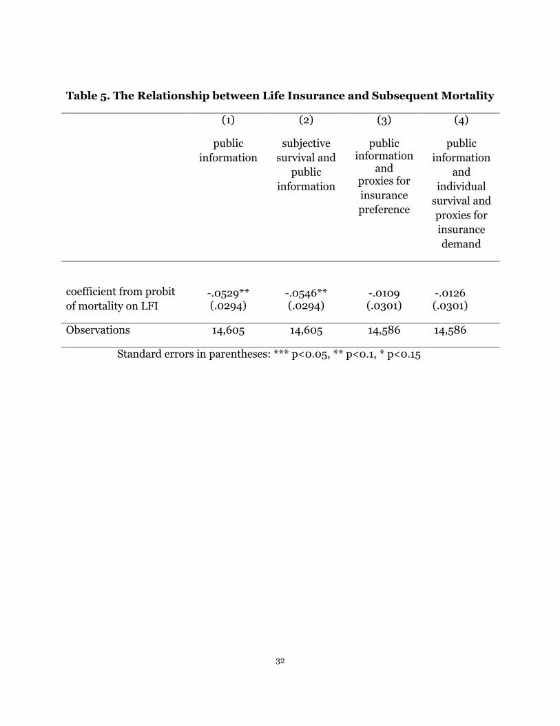
C. Life insurance and individual’s mortality

Another approach, suggested by Finkelstein and Poterba (2004), is also applied

here to confirm this negative or neutral relationship between life insurance purchases

and the mortality we derived above. Table 5 shows the estimated coefficients from

probit estimation of subsequent mortality on the ownership of life insurance (equation

(3)). In column (1) of Table 5, we control for the public information that is available to

insurers. The coefficient for life insurance is negative and statistically significant at -

0.053 (0.029), indicating that individuals who have life insurance are 2% less likely to

die than those who do not. In the second column of Table 5, we add proxy for private

information, i.e., the self-perceived risk of mortality. A similar result is obtained. The

third and fourth columns in Table 5 report the results with proxies for individuals’

preferences in life insurance added, where the fourth column includes self-perceived

risk while column (3) does not. We find that the estimated coefficient for life insurance,

unsurprisingly, is still not significantly different from zero.

D. Identification of private information about mortality using mixture density

model

We now estimate the mixture density model as shown in equation (7), assuming

individuals can be categorized into two types based on their different insurance

preferences. Let H=1 be h type, and H=0 be l type. As discussed before, we cannot

observe which type the individual belongs to, but we can use a series of proxy variables

W which are related to H to probabilistically determine the type of an arbitrary

individual. We then use ML method to estimate our log likelihood function (10).

Column (1) of the top panel of Table 6 reports the estimated effects of the series of

socioeconomic factors predicting the type of an individual. Overall, 86 percent of

individuals belong to the h type.

18

Not surprisingly, people who belong to different types are quite different in their

behaviors. As expected, with everything equal, individuals who are h type are more

likely to purchase life insurance but less likely to experience mortality. For an h-type

individual, the average likelihood of purchasing life insurance is 0.779 and the

probability of mortality is 0.079; while, for an l-type person, the average likelihood of

purchasing life insurance is 0.178 and the probability of mortality is 0.19. In other

words, the h type is 60 percentage points more likely to purchase life insurance but 11

percentage points less likely to experience mortality than the l type.

The conclusion above can also be confirmed from the perspective of the magnitude

of constant terms. For the Die model, with everything equal, the magnitude of the

estimated constant for the h type hc is -0.2888 (3.1764), which is smaller than the

estimated constant for the l type lc at 0.2451 (3.1754). However, for the LFI model,

with everything equal, the magnitude of the estimated constant for h type hc is -3.8322

(2.5344), which is larger than the estimated constant for the l type lc at -5.5241

(2.5530), although they are not significantly different. It is worth mentioning here that

all the results are consistent with the predictions made in Implication 1, the

assumption that guaranteed the point identification of this model.

Most importantly, by distinguishing individuals into h and l types based on their

different preferences in life insurance, we obtain direct evidence of private information

from the standard test. The estimated correlation between the error terms in Die

model and LFI model is, respectively, positive at 0.114 (0.0568) for h-type and 0.327

(0.0777) for l-type individuals, which are both statistically significant at the 5 percent

level. Note that such positive correlation is achieved without using any data on private

information.

In the second column of Table 6, we include one dimension of private information,

the self-perceived probability of being alive for next ten to fifteen years, in both the Die

equation and LFI equation. Consistent with the results reported in one type model in

Table 4, the coefficient of this variable is negative and statistically significant in both

equations, indicating that private information still plays a key role in determining the

purchases of life insurance and predicting subsequent mortality after controlling the

19

classification of risk calculated by insurance companies. We find when adding one

proxy variable for private information, the correlation between the two error terms for

h type and l type are still significantly positive at 0.112 (0.0564) and 0.334 (0.0790),

respectively. All other estimates are similar to the results reported in column (1) of

Table 6.

E. A specification test

In this section, we focus on the test of the key assumption (Assumption 2) which

ensures the full exclusion of such heterogeneity in insurance preferences through the

mixture density model. Given the above assumptions, the probability of mortality and

life insurance purchases conditional on each type can be expressed in the following

forms:

Pr( 1| , ) ( )h

h XDie X H H c X , and Pr( 1| , ) ( )h

h XLFI X H H c X ;

Pr( 1| , ) ( )l

l XDie X H H c X , and Pr( 1| , ) ( )l

l XLFI X H H c X .

Provided that ( , ) 0corr X W , Assumption 2 holds if and only if for any arbitrary

two sets of proxy variable, say Wa and Wb , there is no significantly different estimation

of hc , lc , hc , lc , X and X when using Wa and Wb to determine the types of

individuals, respectively. This enlightens the specification test which is similar to the

over-identification test in the instrumental model when more than one dimension of

instrumental variables W is available. Such method to test Assumption 2 in our paper

is also suggested by HKS. We therefore vary the variables we used in the type equation

as a test of Assumption 2. Specifically, in the present setting, the set of W includes

individuals’ characteristics from five aspects: bequest motives, risk aversion, education,

employment status, and financial conditions. We would like to respectively exclude

each of these five aspects in our specification tests.

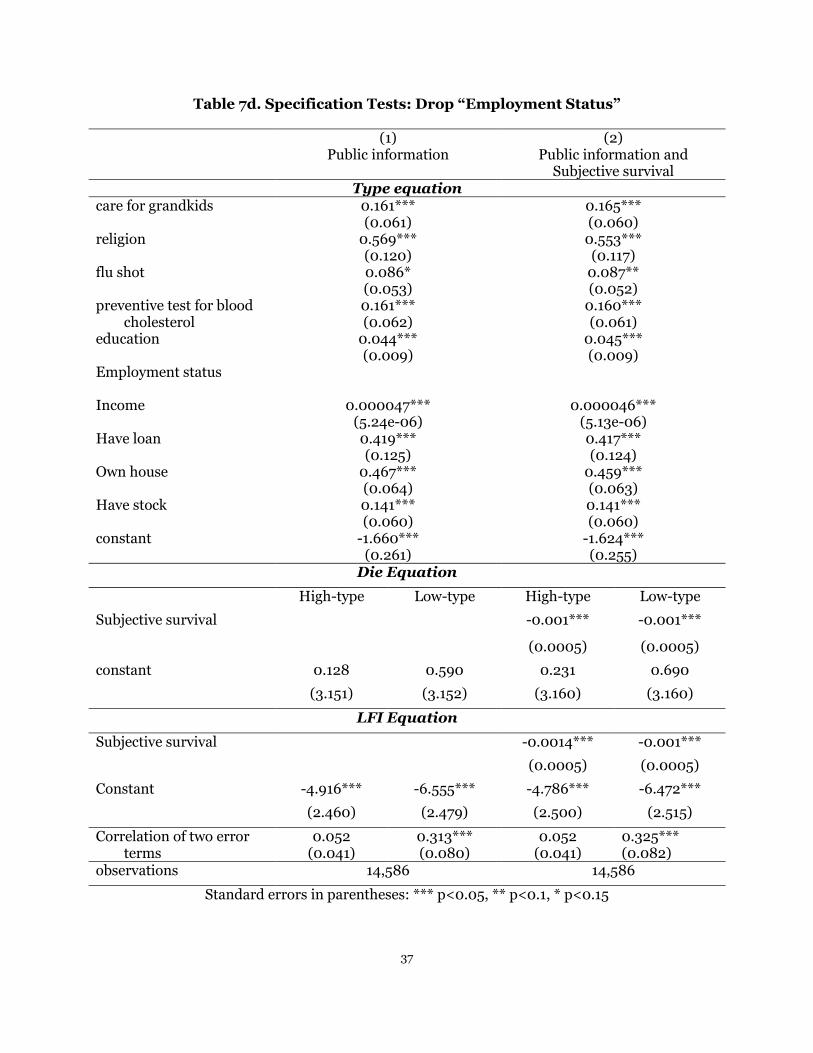
Table 7 (a), (b), (c), (d) and (e) reports the result when proxy variables for bequest

motives, risk attitudes, the number of years of education, employment status and

financial conditions are excluded, respectively, where the first column only includes

public information, X, while the second column includes both public information, X,

and private information on subsequent mortality in next ten to fifteen years, Z. We see

20

under all of these five settings, the constants in both equations satisfy the predictors of

two-type model; parameters in both Die and LFI equations are similar to the

corresponding parameters estimated in Table 6, when a full set of W is used. Moreover,

the correlations between the error terms in Die and LFI equations are still significantly

positive for most of specifications; although such positive correlation is not significant

in case (d) for h type and case (e) for l type.

Table 8 presents a formal Hausman-type test comparing the estimated parameters

of interest in the Die and LFI equations (i.e.,

hc , lc , hc , lc , X and

X ) presented in

Table 7 with each of the five cases in Table 8. Results under five specifications, which

correspond to the specification test in Table 8, are reported. In the first to fifth set of

columns, we compare the estimates from the full model with the bequest motive-

excluded model, risk aversion-excluded model, education-excluded model,

employment status-excluded model, and financial conditions-excluded model,

respectively. The first and second rows compare the parameter estimates in Die

equation and LFI equation, respectively. As expected, estimates in the Die and LFI

equations in all five settings are not significantly different from the parameters

estimated from the full model.

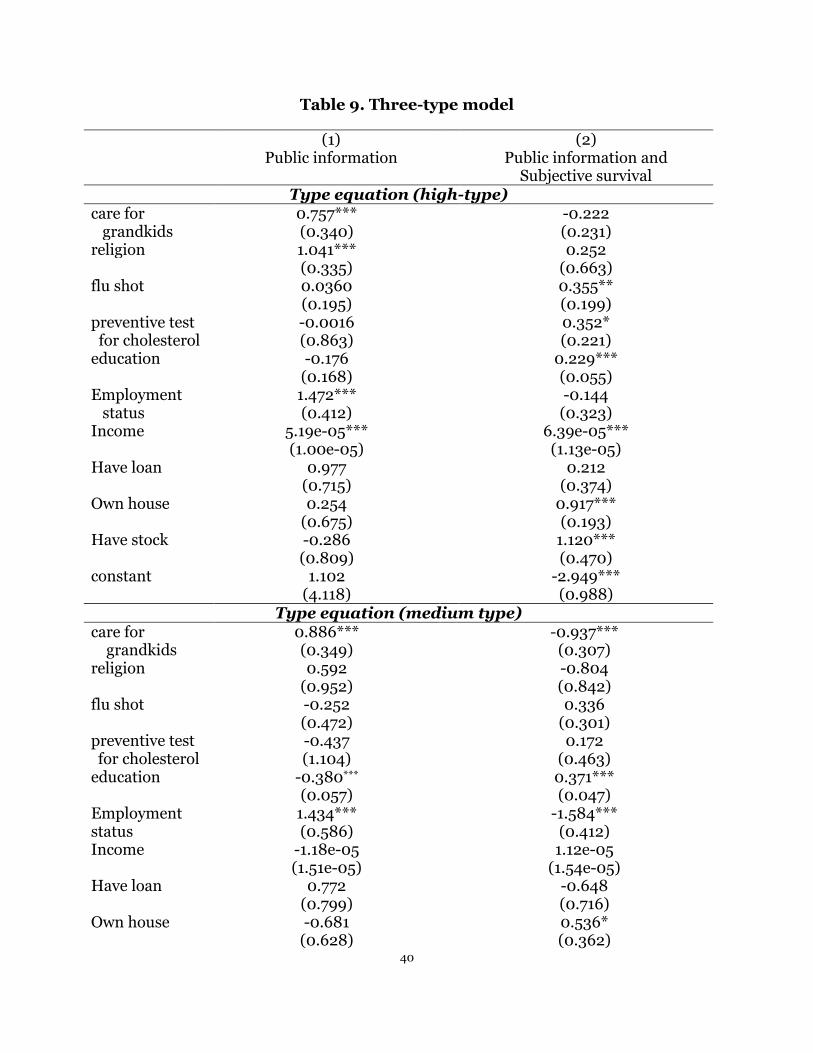
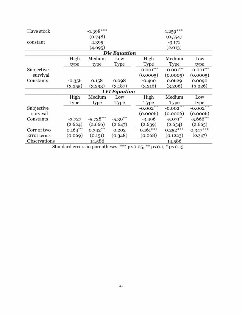
F. A three-type model

Section D and E present results from of the mixture density model with the

assumption that individuals’ heterogeneity in life insurance preferences (H) is

categorized into two types, although, it is possible to categorize them into three or

more types. We distinguish people into three types based on their high, medium, or

low preference for life insurance by using the same set of variables we employed when

separating individuals’ preferences in life insurance into two types, with the

assumption that the probability of being each type has a multinomial logit distribution.

Meanwhile, we make the same restrictions in the two-type model: X and X are set to

be identical for each type, while the correlation between the two error terms in each

type as well as the constant terms are allowed to differ. Table 9 shows the results

estimated from a three-type model, where column (1) includes only public information

21

and column (2) contains both public information as well as self-perceived probability

of being alive for next 10 to 15 years.

We find the correlations between the error terms in Die and LFI equation in each

type are still significantly positive, which are 0.164 (0.069), 0.342 (0.151), and 0.202

(0.348), respectively, when only public information is included. However, compared to

the two-type model, many of the variables used to distinguish people’s heterogeneous

preferences in life insurance in the three-type model become insignificant, indicating

the delimitation of individuals’ different preferences for life insurance is not that clear

when separating individuals into three types by the same set of variables we used for

two types. In other words, there exists much more in common on the taste for life

insurance between each two types of individuals when we categorize individuals into

three types than when we separate them into two.

Next, we apply the Akaike Information Criterion (AIC) and Bayesian Information

Criterion (BIC) as a further comparison of the relative goodness of fit between two-

type and three-type model. Results are shown in Table 10. We find that when there is

only public information added into the Die and LFI equations, the value of AIC is

27375.7 for three-type model, while for two-type model is 27456.9, suggesting that the

three-type model minimizes the information loss compared to the two-type model and

thus is preferred by AIC. However, after introducing a larger penalty term for the

number of parameters, the two-type model is more favorably suggested by BIC. The

corresponding value of BIC for two-type model is 28170.2, while for three-type model

it is 28195.1. The same conclusions can be made when both public and private

information are included in Die and LFI equations. However, since the difference of

values between Two-type and Three-type model measured by both AIC and BIC is

quite small, we may conclude that increasing the number of types does not help

improve the model a lot.

IV. Conclusions

This paper makes three contributions to the literature. First, we find after

controlling the insurer’s risk classification, an individual’s subjective belief of being

alive for next 10 to 15 years still is a significantly negative predictor on subsequent

22

mortality, indicating the existence of residual private information in life insurance

markets. Besides, this residual private information is negatively correlated with the

purchase of life insurances. Combined, these two results provide direct evidence of the

asymmetric information. However, this private information cannot be directly detected

by the standard test which is widely used in most literature.

Second, this paper demonstrates that a series of socioeconomic factors such as

education level, employment status, risk attitudes, bequest motives as well as financial

conditions which result in individuals’ heterogeneity in insurance preferences all have

offsetting effects on life insurance coverage and risk occurrence. Specifically,

individuals who are employed, wealthier, more risk averse, with strong bequest

motives and higher education level as well as those who have stock, loans and houses

are more likely to purchase life insurance but less likely to die. However, even after

controlling these variables, we still cannot observe a positive correlation between life

insurance ownership and subsequent mortality.

Third, by applying the mixture density model, in which we distinguish people into

two unobserved categories based on their different preferences in insurance, we

successfully detect a significantly positive correlation between life insurance purchases

and subsequent mortality, providing a direct evidence of private information suggested

by the standard test.

One direction for future work is to use more diverse distribution assumptions on

the error terms to serve as a further test of our result. In this paper, we estimate our

model by assuming a standard normal distribution of error terms; however, more

extensive distribution assumptions on error terms are welcomed to be applied to

secure a more robust result.

23

References:

American Council of Life Insurers (2010): “2010 Life Insurers Fact Book”

Beck, Thorsten, and Ian Webb (2003): “Economic, demographic, and institutional

determinants of life insurance consumption across countries.” The World Bank

Economic Review, Vol.17, No.1 51-58

Browne, M.J., and K. Kim (1993): “An international analysis of life insurance demand,

Journal of Risk and Insurance,” 60(4): 616-634.

Cawley, John and Tomas Philipson (1999): “An empirical examination of information

barriers to trade in insurance.” American Economic Review, 1999, 89 (4), pp.827-

846

Chiappori, Pierre-Andre (2000): “Econometric models of insurance under asymmetric

information.” In Georges Dionne, ed. Handbook of Insurance Economics. London:

Kluwer

Chiappori, Pierre-Andre and Bernad Salanié (1997): “Empirical contract theory: the case

of insurance data.” European Economic Review, page 943-950

Chiappori, Pierre-André, and Bernard Salanié (2013): “Asymmetric information in

insurance markets: predictions and tests.” Forthcoming in G. Dionne, ed. Handbook

of Insurance, 2nd edition.

Chiappori, Pierre-Andre, and Bernard Salanié (2000): “Testing for asymmetric

information in insurance markets.” Journal of Political Economy, 108 (1), page 56-78

Chiappori, Pierre-Andre, Bruno Jullien, Bernard Salanié, and Francois Salanié (2006):

“Asymmetric information in insurance: general testable implications.” The RAND

Journal of Economics, Vol 37, Issue 4, pages 783–798

Cutler, David, Amy Finkelstein and Kathleen McGarry (2008): “Preference

heterogeneity and insurance markets: explaining a puzzle of insurance.” American

Economic Review: Papers and Proceedings, 98:2, page 157-162

Fang, Hanming, Michael P. Keane, and Dan Silverman (2008): “Sources of

advantageous selection: evidence from the Medigap insurance market.” Journal of

Political Economy, Volume 116, Issue 2, page 303-350

Finkelstein, Amy and Kathleen McGarry (2006): “Multiple dimensions of private

information: evidence from the long-term care insurance market.” American

Economic Review, Vol.96 No.4, page 938-958

24

Finkelstein, Amy and James Poterba (2002). “Selection effects in the market for

individual annuities: new evidence from the United Kingdom.” Economic Journal,

2002, 112 (476), pp. 28-50.

Gan, Li, Michael Hurd and Daniel McFadden (2005): “Individual subjective survival

curves.” In David Wise, ed., Analysis in Economics of Aging. Chicago: University of

Chicago Press, page 377-411

Gan, Li, Feng Huang and Adalbert Mayer (2010): “A simple test of private information

in the insurance markets with heterogeneous insurance demand.” NBER WPS

#16738

Gan, Li, Guan Gong, Michael Hurd, and Danie McFadden (2013): “Individual subjective

survival curves and bequests.” Forthcoming, Journal of Econometrics.

Gan, Li and Manuel Hernandez (2013): “Making friends with your neighbors?

Agglomeration and tacit collusion in the lodging industry.” Review of Economics and

Statistics, July 2013, 95(3): 1002-1017.

Hakansson, Nils H. (1969). “Optimal investment and consumption strategies under risk,

an uncertain life time, and insurance.” International Economic Review, Vol. 10, No. 3

Oct, 1969, pp. 443-466.

He, Daifeng (2009). “The life insurance market: asymmetric information revisited”

Journal of Public Economics, Vol 93, Issues 9-10, Oct 2009, pp. 1090-1097.

Hendel, Igal, and Alessandro Lizzie (2003). “The role of commitment in dynamic contracts: evidence from life insurance.” The Quarterly Journal of Economics, Vol. 118, No. 1, pp. 299-327

Henry, Marc, Yuichi Kitamura, and Bernard Salanié (2010). “Identifying finite mixtures

in econometric models” Cowles Foundation Discussion Paper #1767

Hu, Yingyao (2008). “Identification and estimation of nonlinear models with

misclassification error using instrumental variables: A general solution” Journal of

Econometrics, 144, 27–61

Hurd, Michael D. and McGarry, Kathleen (2002). "The Predictive validity of subjective

probabilities of survival." Economic Journal, 2002, 112(482), pp. 966-85

Jullien, Bruno, Bernard Salanié and François Salanié (2007). “Screening risk-averse agents under moral hazard: single-crossing and the CARA case.” Economic Theory, Vol. 30, No. 1, pp. 151-169

Lewis, Frank D. (1989). “Dependents and the demand for life insurance” The American

25

Economic Review, Vol. 79, No. 3, pp. 452-467 Mahajan, Aprajit (2006). “Identification and estimation of regression models with

misclassification.” Econometrica, Vol.74, No.3 631-665

Meza, David de and David C. Webb (2001). “Advantageous selection in insurance

markets.” The RAND Journal of Economics, 32 (2), page 249-262

Pauly, Mark V., Kate H. Withers, Krupa Subramanian-Viswana, Jean Lemaire, and John

C. Hershey (2003). “Price elasticity of demand for term life insurance and adverse

selection” NBER WPS #9925

Rothschild, Michael and Joseph Stiglitz (1976) “Equilibrium in competitive insurance

markets: an essay on the economics of imperfect information.” Quarterly Journal of

Economics, 1976, 90 (4) pp. 629-649.

Smart, Michael (2000) “Competitive insurance markets with two unobservables.”

International Economic Review, 2000, 41(1) pp. 153-169.

Walliser, Jan and Joachim K. Winter (1998). “Tax incentives, bequest motives and the

demand for life insurance: evidence from Germany” Working Paper.

Yarri, Menahem E. (1965). “Uncertain life time, life insurance, and the theory of the

consumer” The Review of Economic Studies, Vol. 32, No. 2, pp. 137-150

http://www.nber.org/people/mark_pauly

26

Table 1. Unconditional Relationship between Life Insurance

Life insurance ownership

0 1 Sum

Die

0 22.7% 56.7% 79.4%

1 7.8% 12.8% 20.6%

Sum 30.5% 69.5%

Table 2. Thought Experiment

Group Number Probability of

Mortality

Purchase of Life

Insurance

Low insurance

preference

group (l)

1 20 1

2 30 1

3 40 2

4 50 3

5 60 4

High insurance

preference

group (h)

A 10 1

B 20 2

C 30 2

D 40 3

E 50 4

All together

10 1

20 2

30 3

40 5

50 7

60 4

27

28

Table 3. Summary of Statistics

Variables Mean Std. Deviation Min Max

Die 0.21 0.41 0 1

LFI 0.7 0.46 0 1

Subjective survival 49.51 31.75 0 100

Marriage 0.69 0.46 0 1

Spouse age 44.49 30.87 0 99

age 65.92 9.97 27 90

age square 4444 1334 729 8100

age cubic 306172 137461 19683 729000

black 0.12 0.32 0 1

age x black 7.6 21.01 0 90

age square x black 499 1430 0 8100

age cubic x black 33482 101661 0 729000

age x gender 26.56 33.14 0 90

age square x gender 1804 2353 0 8100

age cubic x gender 124801 174154 0 72900

male 0.4 0.49 0 1

arthritis 0.56 0.5 0 1

high blood pressure 0.48 0.5 0 1

lung 0.09 0.29 0 1

cancer 0.12 0.33 0 1

heart 0.21 0.41 0 1

stroke 0.06 0.23 0 1

drink 0.06 0.24 0 1

smoke now 0.16 0.36 0 1

smoke ever 0.6 0.49 0 1

diabetes 0.17 0.44 0 1

incontinent 0.17 0.38 0 1

psych 0.14 0.34 0 1

depression 0.23 0.42 0 1

back 0.33 0.47 0 1

self-reported-health 3.3 1.11 1 5

BMI 27.25 5.34 12.6 75.5

take drugs 0.77 0.42 0 1

home care use 0.05 0.23 0 1

nursing home 0.01 0.12 0 1

hospital 0.23 0.42 0 1

number of kid 3.25 2.15 0 20

kid 0.94 0.25 0 1

29

No of siblings 2.59 2.31 0 17

siblings 0.85 0.36 0 1

No of grandkids 5.07 5.43 0 80

grandkid 0.8 0.4 0 1

care grandkid missing 0.2 0.4 0 1

care for grandkid 0.28

0.45

0 1

religion 0.95

0.23

0 1

education 12.47

3.02

0 17

flu shot 0.61

0.49

0 1

test for blood 0.77 0.42 0 1

employment 0.4

0.49

0 1

stock 0.36

0.48

0 1

loan 0.08

0.27

0 1

income ($) 21793 33167 0 2000000

30

Table 4. One Type Bivariate Probit Model

(1) (2) (3) (4)

public information

subjective survival and

public information

public information and proxies

for insurance preference

public information

and individual survival and proxies for insurance demand

Die equation

subjective survival -0.0011*** -0.0010***

(0.0005) (0.0005)

care for grandkids -0.0948*** -0.0945***

(0.0344) (0.0344)

religion -0.0986** -0.0989**

(0.0600) (0.0600)

flu shot 0.0135 0.0138

(0.0316) (0.0316)

preventive test for blood

cholesterol

-0.217***

(0.0354)

-0.215***

(0.0354)

education -0.0004 -0.0002

(0.0052) (0.0052)

employment status -0.159*** -0.156***

(0.0361) (0.0361)

income -1.31e-06** -1.33e-06**

(7.21e-07) (7.21e-07)

have loan -0.0060 -0.0043

(0.0587) (0.0587)

own house -0.134*** -0.134***

(0.0368) (0.0368)

have stock -0.0887*** -0.0887***

(0.0320) (0.0320)

constant 0.0658 0.160 -0.882 -0.792

(3.1753) (3.189) (3.185) (3.196)

LFI equation

subjective survival -0.0008*** -0.0011***

(0.0004) (0.0004)

care for grandkids 0.0807*** 0.0814***

(0.0279) (0.0279)

religion 0.230*** 0.230***

(0.0496) (0.0496)

flu shot 0.0674*** 0.0679***

(0.0256) (0.0256)

31

preventive test for blood

cholesterol

0.0657***

(0.0287)

0.0677***

(0.0287)

education 0.0278*** 0.0284***

(0.0044) (0.0044)

Employment status 0.334*** 0.335***

(0.0285) (0.0285)

income 2.94e-06*** 2.94e-06***

(3.91e-07) (3.91e-07)

have loan 0.188*** 0.190***

(0.0466) (0.0467)

own house 0.257*** 0.256***

(0.0316) (0.0316)

have stock 0.0413* 0.0418*

(0.0261) (0.0262)

constant -5.1930*** -5.084*** -3.417** -3.272**

(1.8514) (1.852) (1.925) (1.926)

corr of two error terms -0.0331**

(0.0178)

-0.0341**

(0.0178)

-0.00573

(0.0182)

-0.00678

(0.0182)

observations 14,605 14,605 14,586 14,586

Standard errors in parentheses: *** p<0.05, ** p<0.1, * p<0.15

32

Table 5. The Relationship between Life Insurance and Subsequent Mortality

(1) (2) (3) (4)

public

information

subjective

survival and

public

information

public information

and proxies for

insurance

preference

public

information

and

individual

survival and

proxies for

insurance

demand

coefficient from probit

of mortality on LFI

-.0529** (.0294)

-.0546** (.0294)

-.0109 (.0301)

-.0126 (.0301)

Observations 14,605 14,605 14,586 14,586


33

Table 6. Mixture density model (Two-type)

(1) Public information

(2) Public information and

Subjective survival Type equation

care for grandkids 0.1686*** 0.1679*** (0.0563) (0.0558) religion 0.5295*** 0.5216*** (0.1075) (0.1060) flu shot 0.0988*** 0.0995*** (0.0492) (0.0488) preventive test for blood cholesterol

0.1764*** (0.0577)

0.1767*** (0.0571)

education 0.0334*** 0.0343*** (0.0086) (0.0086) Employment status 0.3990***

(0.0631) 0.3925*** (0.0628)

Income 3.52e-05*** 3.5e-05*** (4.38e-06) (4.31e-06) Have loan 0.3656*** 0.3665*** (0.1120) (0.1114) Own house 0.4276*** 0.4226*** (0.0607) (0.0560) Have stock 0.1057*** 0.1062*** (0.0534) (0.0530) constant -1.5840*** -1.569*** (0.2459) (0.2436)

Die Equation

High-type Low-type High-type Low-type

Subjective survival -0.0011*** -0.0011***

(0.0005) (0.0005)

constant -0.2888 0.2451 -0.1787 0.3522

(3.1764) (3.1754) (3.1831) (3.1821)

LFI Equation


(0.0005) (0.0005)

Constant -3.8322* 5.5241*** -3.671 -5.389***

(0.0568) (0.0777) (2.5556) (2.5751)

Correlation of two error terms

0.114*** (0.0568)

0.327*** (0.0777)

0.112*** (0.0564)

0.334*** (0.0790)

observations 14,586 14,586 14,586 14,586


34

Table 7a: Specification Tests: Drop “Bequest motives”




care for grandkids religion flu shot 0.0985***

(0.048) 0.0996*** (0.0477)

preventive test for blood cholesterol

0.1730*** (0.057)

0.1727*** (0.056)

Education 0.033*** 0.034***

(0.008) (0.008) Employment status 0.0379*** 0.371*** (0.0619) (0.0615) Income 0.0000359*** 0.0000356*** (4.51e-06) (4.45e-06) Have loan 0.357*** 0.358*** (0.113) (0.112) Own house 0.430*** 0.425*** (0.059) (0.058) Have stock 0.112*** 0.113*** (0.053) (0.053) constant -0.980*** -0.968*** (0.181) (0.179)

Die Equation



(0.0004) (0.0004)

constant -0.0168 0.4897 0.093 0.594

(3.166) (3.165) (3.171) (3.171)

LFI Equation

Subjective survival -0.0015*** -0.0015*

(0.0005) (0.0005)

Constant -4.857** -6.632*** -4.729** -6.543**

(2.597) (2.626) (2.622) (2.654)


0.106*** (0.0529)

0.338** 0.103*** 0.348***

observations 14,586 14,586 14,586 14,586


35

Table 7b. Specification Tests: Drop “Risk Averse” (1)

Public information (2)

Public information and Subjective survival

Type equation care for grandkids 0.168*** 0.167***

(0.056) (0.056) religion 0.523*** 0.516*** (0.107) (0.106) flu shot preventive test for blood cholesterol

education 0.035*** 0.036*** (0.0086) (0.008) Employment status 0.371*** 0.365*** (0.062) (0.062) Income 0.000036*** 0.000036*** (4.55e-06) (4.48e-06) Have loan 0.370*** 0.371*** (0.112) (0.111) Own house 0.427*** 0.423*** (0.061) (0.060) Have stock 0.116*** 0.116*** 0.052) (0.052) constant -1.392 -1.377 (0.242) (0.240)

Die Equation



(0.0005) (0.0005)

constant -0.266 0.225 -0.162 0.327

(3.178) (3.177) (3.183) (3.182)

LFI Equation


(0.0005) (0.0005)

Constant -3.911* -5.650*** -3.760* -5.524***

(2.567) (2.591) (2.588) (2.613)


0.110*** (0.056)

0.307*** (0.083)

0.107*** (0.055)

0.313*** (0.084)

observations 14,586 14,586 14,586 14,586


36

Table 7c. Specification Tests: Drop “Education”





0.194*** (0.0594)

0.195*** (0.0591)

education 0.432*** 0.428*** (0.064) (0.063) Employment status Income 0.000036*** 0.000036*** (4.31e-06) (4.26e-06) Have loan 0.3837*** 0.3860*** (0.113) (0.112) Own house 0.446*** 0.443*** (0.062) (0.062) Have stock 0.140*** 0.141*** (0.053) (0.053) constant -1.308*** -1.294*** (0.225) (0.224)

Die Equation



(0.0005) (0.0005)

constant -0.599 -0.053 -0.499 0.046

(3.185) (3.184) (3.194) (3.193)

LFI Equation


(0.0005) (0.0005)

Constant -.852*** -5.456*** -3.677*** -5.296***

(2.458) (2.471) (2.470) (2.483)


0.118*** (0.060)

0.301*** (0.074)

0.116** (0.060)

0.305*** (0.074)

observations 14,586 14,586


37

Table 7d. Specification Tests: Drop “Employment Status”




care for grandkids 0.161*** 0.165*** (0.061) (0.060) religion 0.569*** 0.553*** (0.120) (0.117) flu shot 0.086* 0.087** (0.053) (0.052) preventive test for blood cholesterol

0.161*** (0.062)

0.160*** (0.061)

education 0.044*** 0.045*** (0.009) (0.009) Employment status Income 0.000047*** 0.000046*** (5.24e-06) (5.13e-06) Have loan 0.419*** 0.417*** (0.125) (0.124) Own house 0.467*** 0.459*** (0.064) (0.063) Have stock 0.141*** 0.141*** (0.060) (0.060) constant -1.660*** -1.624*** (0.261) (0.255)

Die Equation



(0.0005) (0.0005)

constant 0.128 0.590 0.231 0.690

(3.151) (3.152) (3.160) (3.160)

LFI Equation


(0.0005) (0.0005)

Constant -4.916*** -6.555*** -4.786*** -6.472***

(2.460) (2.479) (2.500) (2.515)


0.052 (0.041)

0.313*** (0.080)

0.052 (0.041)

0.325*** (0.082)

observations 14,586 14,586


38

Table 7e. Specification Tests: Drop “Financial Conditions”





0.336*** (0.097)

0.333*** (0.096)

education 0.084*** 0.084*** (0.017) (0.018) Employment status 0.935*** 0.921*** (0.179) (0.181) Income Have loan Own house Have stock constant -1.973*** -1.958*** (0.607) (0.620)

Die Equation


Subjective survival -0.001 -0.001

(0.0005) (0.0005)

constant -1.115 -0.531 -1.000 0.420

(3.297) (3.297) (3.299) (3.299)

LFI Equation

Subjective survival --0.0013*** --0.0013***

(0.0005) (0.0005)

Constant -2.284 -4.035*** -3.884

(2.215) (2.259) (2.281)


0.225*** (0.082)

0.114 (0.104)

0.223*** (0.082)

0.118 (0.110)

observations 14,586 14,586 14,586 14,586


39

Table 8. Hausman Tests: The Baseline Model vs Models with

Only a Subset of Proxy Variables for Insurance Demand

Baseline model vs

Drop “Bequest Motives”

Baseline model vs

Drop “Risk Averse”

Baseline model vs

Drop “Education”

Public

information

Public and

subjective

survival

Public

information

Public and

subjective

survival

Public

information

Public &

subjective

survival

Die 5.46 5.13 4.12 4.19 0.06 6.87

equation (1.000) (1.000) (1.000) (1.000) (1.000) (1.000)

LFI 16.24 11.31 18.06 17.76 14.74 14.60

equation (0.991) (1.000) (0.977) (0.980) (0.996) (0.996)

Baseline model vs

Drop “Employment

status”

Baseline model vs

Drop “Financial

Condition”

Public

information

Public and

subjective

survival

Public

information

Public and

subjective

survival

Die 5.87 5.62 9.58 0.79

equation (1.000) (1.000) (1.999) (1.000)

LFI 11.94 14.73 9.93 6.20

equation (1.000) (0.996) (0.999) (1.000)

40

Table 9. Three-type model



Subjective survival Type equation (high-type)

care for grandkids

0.757*** (0.340)

-0.222 (0.231)

religion 1.041*** 0.252 (0.335) (0.663) flu shot 0.0360 0.355** (0.195) (0.199) preventive test for cholesterol

-0.0016 (0.863)

0.352* (0.221)

education -0.176 0.229*** (0.168) (0.055) Employment status

1.472*** (0.412)

-0.144 (0.323)

Income 5.19e-05*** 6.39e-05*** (1.00e-05) (1.13e-05) Have loan 0.977 0.212 (0.715) (0.374) Own house 0.254 0.917*** (0.675) (0.193) Have stock -0.286 1.120*** (0.809) (0.470) constant 1.102 -2.949*** (4.118) (0.988)

Type equation (medium type) care for grandkids

0.886*** (0.349)

-0.937*** (0.307)

religion 0.592 -0.804 (0.952) (0.842) flu shot -0.252 0.336 (0.472) (0.301) preventive test for cholesterol

-0.437 (1.104)

0.172 (0.463)

education -0.380*** 0.371*** (0.057) (0.047) Employment status

1.434*** (0.586)

-1.584*** (0.412)

Income -1.18e-05 1.12e-05 (1.51e-05) (1.54e-05) Have loan 0.772 -0.648 (0.799) (0.716) Own house -0.681 0.536* (0.628) (0.362)

41

Have stock -1.398*** 1.259*** (0.748) (0.554) constant 4.395 -3.171 (4.695) (2.013)

Die Equation High

type Medium

type Low Type

High Type

Medium Type

Low type

Subjective survival

-0.001***

(0.0005) -0.001***

(0.0005) -0.001***

(0.0005) Constants -0.356 0.158 0.098 -0.460 0.0629 0.0090 (3.255) (3.293) (3.187) (3.216) (3.206) (3.226)

LFI Equation High

type Medium

type Low Type

High Type

Medium Type

Low type

Subjective survival

-0.002***

(0.0006) -0.002***

(0.0006) -0.002***

(0.0006) Constants -3.727 -5.728*** -5.30*** -3.496 -5.071** -5.666*** (2.624) (2.666) (2.647) (2.639) (2.654) (2.665) Corr of two

Error terms 0.164***

(0.069) 0.342***

(0.151) 0.202

(0.348) 0.161***

(0.068) 0.252***

(0.1223) 0.347***

(0.347)

Observations 14,586 14,586 Standard errors in parentheses: *** p<0.05, ** p<0.1, * p<0.15

42

Table 10. A Comparison of the Goodness of Fit between Two-type model and

Three-type model via Akaike Information Criterion (AIC) and Bayesian

Information Criterion (BIC)

AIC

Two-Type Model Three-Type Model

w/o private information 27456.9 27375.7

With private information 27447.8 27365.5

BIC

Two-Type Model Three-Type Model

w/o private information 28170.2 28195.1

With private information 28176.3 28200.1

Documents

A Test of Private Information in Life Insurance Markets