A TEST FOR MONOTONE COMPARATIVE STATICS

A TEST FOR MONOTONE COMPARATIVE STATICS

FEDERICO ECHENIQUE AND IVANA KOMUNJER

Abstract. In this paper we design an econometric test for monotone comparative

statics (MCS) often found in models with multiple equilibria. Our test exploits the

observable implications of the MCS prediction: that the extreme (high and low)

conditional quantiles of the dependent variable increase monotonically with the

explanatory variable. The main contribution of the paper is to derive a likelihood-

ratio test, which to the best of our knowledge, is the first econometric test of MCS

proposed in the literature. The test is an asymptotic “chi-bar squared” test for

order restrictions on intermediate conditional quantiles. The key features of our ap-

proach are: (1) it does not require estimating the underlying nonparametric model

relating the dependent and explanatory variables to the latent disturbances; (2) it

makes few assumptions on the cardinality, location, or probabilities over equilib-

ria. In particular, one can implement our test without assuming an equilibrium

selection rule.

JEL codes: C12, C51

Keywords: multiple equilibria, comparative statics, quantiles, “chi-bar squared”

Affiliations and Contact information. Echenique: Division of the Humanities and Social Sciences,

California Institute of Technology, 1200 E California Bvd, Pasadena CA 91125, Phone: (626) 395-

4273, Fax: (626) 793-8580, E-mail: [email protected]. Komunjer: Department of Economics,

University of California at San Diego, 9500 Gilman Dr, La Jolla CA 92093-0508, Phone: (858)

822-0667, Fax: (858) 534-0172, E-mail: [email protected].

A TEST FOR MONOTONE COMPARATIVE STATICS 1

1. Introduction

Comparative statics predictions—or how exogenous variables affect endogenous

variables—are important to establish in economic models.1 Often, the models pos-

sess multiple equilibria, and a monotone comparative statics (MCS) prediction holds:

There is a smallest and a largest equilibrium, and these change monotonically with

explanatory variables (see, e.g., Milgrom and Roberts, 1990; Milgrom and Shannon,

1994; Villas-Boas, 1997). MCS is a feature found in many well-known economic mod-

els. Examples are single-person decision models such as models of optimal growth

(see, e.g., Barro and Sala-I-Martin, 2003; Ljungqvist and Sargent, 2004) and firms’

investment decisions (see, e.g., Hayashi, 1982; Hayashi and Inoue, 1991), as well as

many models in IO (see Vives, 1999, for survey). Current econometric literature, on

the other hand, has largely remained silent on the issue of formal tests for MCS.2

The goal of this paper is to fill this gap.

There are two challenges in testing the MCS hypothesis. The first is to obtain

testable implications; the second is to construct a formal statistical test and study

its properties. In the context of structural models, Echenique and Komunjer (2007)

solve the first, but not the second challenge. They obtain testable implications of

the MCS property in the form of restrictions on the conditional quantiles of the

dependent variable given the explanatory variable.

In this paper, we derive similar restrictions on conditional quantiles in the context

of reduced form models with multiple equilibria. Our main contribution is to show

how to test those restrictions in a way that is not affected by equilibrium selections.

In general, the latter are unknown and have to be treated as nuisance parameters of

1According to Samuelson (1947): “The usefulness of our theory emerges from the fact that byour analysis we are often able to determine the nature of the changes in our unknown variablesresulting from a designated change in one of more parameters.”

2We note that Athey and Stern (1998) discuss tests for monotone comparative statics, however,only in the context of firms’ choice of organizational form.

2 ECHENIQUE AND KOMUNJER

the problem. Our approach is to first estimate the conditional quantiles nonparamet-

rically, then use those to construct an asymptotic likelihood-ratio test of the order

restrictions implied by the MCS. The test relies only on the asymptotic distribution

results; it is an extension of the “chi-bar squared” test by Gourieroux, Holly, and

Monfort (1982) and Kodde and Palm (1986) to restrictions on conditional quantiles.

In the remainder of this Introduction, we give a brief overview of the related

literature, and present an example of how one could use our results.

Related Literature. As early as in the work of Bjorn and Vuong (1984, 1985),

econometricians recognized the importance of testing economic models that possess

multiple equilibria. Proposed solutions to the problem of multiplicity have been to

assume the probabilities of various equilibrium realizations known (see, e.g., Bjorn

and Vuong, 1984); or finitely parameterized (see, e.g., Bjorn and Vuong, 1985; McK-

elvey and Palfrey, 1995; Bajari, Hong, and Ryan, 2004; Sweeting, 2005). Without

the specification of an equilibrium selection rule, there are alternative approaches to

estimation and inference. The first exploits the fact that—despite the multiplicity—

some of the model features are uniquely predicted (see, e.g., Bresnahan and Reiss,

1990, 1991); by focusing attention on those features, one is then able to carry out

likelihood-based estimation and inference.

The second approach is to work with structural models in which, despite multiplic-

ity, point identification of the structural parameters is known to hold. Observable

implications in models with multiple equilibria were first derived by Jovanovic (1989)

who sought conditions for point identification (see also Aradillas-Lopez and Tamer,

2008; Molinari and Rosen, 2008). When the parameters of interest are only set-

identified, interesting results on estimation and inference can be found in the rapidly

growing literature on econometrics of games (see, e.g., Berry, 1992; Tamer, 2003;

Andrews, Berry, and Jia, 2004; Ciliberto and Tamer, 2004; Kim, 2005). Mostly,


these papers build on discrete-choice methods and are well-suited for models with

few choice variables; our methods, on the other hand, apply to models with con-

tinuous endogenous variables. The goal in those papers is also different than ours:

typically, they try to estimate agents’ payoff functions (i.e. estimate the nature of

strategic interaction); we only test for the presence of a comparative statics effect.

Finally, we want to emphasize the relevance of a rapidly growing literature on

partially identified models (see, e.g., Galichon and Henry, 2006; Chernozhukov,

Hong, and Tamer, 2007; Canay, 2008; Molinari and Beresteanu, 2008) in our context.

Mostly, however, those papers do not explicitly model comparative statics effects:

they focus on general estimation and inference issues.

Example. We now illustrate how to use our results. Say that one is interested

in testing whether an exogenous change in a policy causes the prices in the market

for cars to increase. When there are complementarities between the policy and the

agents’ choice variables, the effect on prices takes the form of MCS. In the case of

car prices, policy changes which increase marginal cost would cause the smallest

and largest equilibria to increase. Examples of these policies are environmental

regulations (Pakes, Berry, and Levinsohn, 1993) and voluntary export restraints

(Berry, Levinsohn, and Pakes, 1999).

Concretely, let Y denote the price and X the policy dummy; further, suppose that

an economic theory posits a reduced form model for Y that has the form Y = g(X)U ,

where one observes an “intended equilibrium” g(X), subject to a multiplicative shock

U .3 Here, g is generally unknown.

Many models which yield predictions for price competition—such as Berry, Levin-

sohn, and Pakes (1995, 1999), for example—are also likely to have multiple equilibria.

3A multiplicative error model is chosen so as to preserve the positivity of the price variable Y .


Before

After

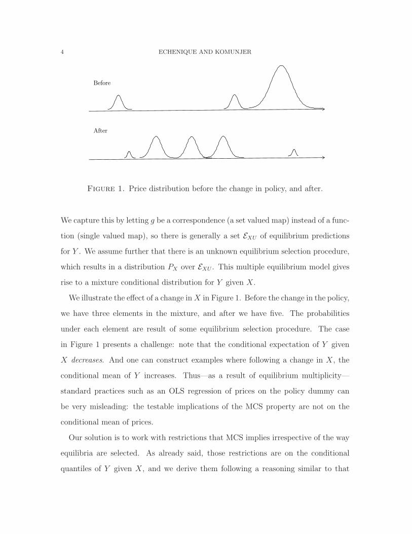
Figure 1. Price distribution before the change in policy, and after.

We capture this by letting g be a correspondence (a set valued map) instead of a func-

tion (single valued map), so there is generally a set EXU of equilibrium predictions

for Y . We assume further that there is an unknown equilibrium selection procedure,

which results in a distribution PX over EXU . This multiple equilibrium model gives

rise to a mixture conditional distribution for Y given X.

We illustrate the effect of a change in X in Figure 1. Before the change in the policy,

we have three elements in the mixture, and after we have five. The probabilities

under each element are result of some equilibrium selection procedure. The case

in Figure 1 presents a challenge: note that the conditional expectation of Y given

X decreases. And one can construct examples where following a change in X, the

conditional mean of Y increases. Thus—as a result of equilibrium multiplicity—

standard practices such as an OLS regression of prices on the policy dummy can

be very misleading: the testable implications of the MCS property are not on the

conditional mean of prices.

Our solution is to work with restrictions that MCS implies irrespective of the way

equilibria are selected. As already said, those restrictions are on the conditional

quantiles of Y given X, and we derive them following a reasoning similar to that


in Echenique and Komunjer (2007). It is important to stress that we make few

assumptions on the true equilibrium distribution. We only assume that PX puts a

positive probability on the extremal equilibria. Similarly, our assumptions on the

distribution of the equilibrium deviations U are weak; we need them to belong to a

well-known class of distributions in extreme-value theory. This class includes most

distributions commonly used in empirical work, such as Gaussian, lognormal and

exponential distributions.

Once the appropriate implications of the MCS hypothesis derived, we proceed with

a construction of a likelihood-ratio test. In particular, our test is a test for order

restrictions on the conditional quantiles of Y given X. We use a two step approach:

first, we construct nonparametric estimators for the conditional quantiles of Y given

X. The key difficulty here is that the MCS prediction holds only for quantiles that are

extreme; hence, we need to use a nonstandard framework to derive their asymptotic

distribution (Dekkers and de Haan, 1989; Chernozhukov, 2005a,b).

In the second step, we construct a likelihood-ratio test for order restrictions based

on the asymptotic distributions of our conditional quantile estimators. This step

presents important challenges as the existing results (Gourieroux, Holly, and Mon-

fort, 1982; Kodde and Palm, 1986) apply only to the conditional means; hence, we

need to extend them to our extreme conditional quantile framework. Perhaps an

even greater difficulty comes from the presence of numerous nuisance parameters—

unknown equilibrium selection probabilities—that we need to eliminate from our test

statistic. Unfortunately, the standard approaches of dealing with nuisance parame-

ters fail to work once we exit the usual asymptotic framework. Our solution is to first

consider the problem in the exact case (as in Bartholomew, 1959a,b, for example),

then extend the obtained solution to our asymptotic framework.


The remainder of the paper is organized as follows: We introduce the model in

Section 2, and present the intuition behind our main results in Section 3. In Section 4

we present the basic statistical framework, and develop an approach to estimation

in Section 5. Finally, in Section 6 we present our test.

2. Setup

2.1. Multiple Equilibrium Model. Consider a familiar nonlinear regression

model with a multiplicative error:

(1) Y = g(X)U

that relates a dependent variable Y ∈ R++, an explanatory variable X ∈ X with

X finite in R, and a latent disturbance U ∈ R++.4 The map g : X → R++ in

Equation (1) is unknown; we assume however that g is positive valued, so that the

positivity of the dependent variable is preserved. When the map g is known up to

some finite dimensional parameter θ, one can write g(X, θ) in Equation (1). While

the explanatory and dependent variables X and Y are observable, the disturbance

U is not; U can be thought of as unaccounted heterogeneity in the model. Finally,

note that the random variables Y and U are assumed to be continuous, whereas X

is restricted to be discrete. Hereafter, we shall use the lowercase letters y, x and u

to denote the realizations of the random variables Y , X and U , respectively.

Underlying the model in Equation (1) is the assumption that, given the explana-

tory variable X, a unique value of the dependent variable Y can be assigned to each

value of the disturbance U . In other words, conditional on X, the mapping from the

unobservables to the observables is single valued, and g in Equation (1) is a function.

4All of our results are easily transposable to additive error models of the form Y = g(X) + U

with Y ∈ R, U ∈ R, X ∈ X and g : X → R, by taking the exponentials.


In models that possess multiple equilibria, this letter property is generally violated

as more than one value of Y can be associated with each value of U .

In order to adapt our model to multiple equilibria for Y , we shall assume that the

map g in Equation (1) is a correspondence g : R ⇒ R++, which, to each x ∈ X ,

assigns the set Γx ≡ {gi(x), . . . , gNx(x) : g1(x) � . . . � gNx(x)}. The maps gi which

define the image set Γx are single valued so every gi : R → R++ is a function. We

do not make any assumptions regarding continuity or differentiability of gi’s except

that they are Borel-measurable. As a result, there are multiple equilibria for the

dependent variable Y in Equation (1) given by Yi = gi(X)U with i = 1, . . . , NX . We

then let EXU ≡ {Y1, . . . , YNX} denote the equilibrium set.5 Note that all equilibria

for Y are ordered in EXU , i.e. Y1 � . . . � YNX. We shall work with the following

definition.

Definition 1. A multiple equilibrium model is a collection (EXU , PX , FU |X) such that

for every (x, x′, u) ∈ X 2 × R++ we have:

(i) Exu ⊆ R++ is finite and nonempty;

(ii) x < x′ implies that min Exu < min Ex′u and max Exu < max Ex′u;

(iii) Px is a probability distribution over Exu, Px(min Exu) > 0 and Px(max Exu) > 0;

(iv)FU |X=x is a twice-differentiable distribution function with positive density on R++.

We assume that EXU ⊆ R++ is finite, so we accommodate multiple, but finitely-

many, equilibria. The assumption is common, and often justified by standard gener-

icity arguments: In parameterized families of economic models, one obtains finitely

many equilibria except on sets of measure zero (see, e.g., Mas-Colell, Whinston,

and Green, 1995). Our results shall build on the comparative statics in item (ii)

of Definition 1: an increase in X causes the smallest and largest equilibria in EXU

5Note that while we explicitly allow the cardinality of the equilibrium set Nx to vary with x,we can also accommodate the case in which the latter varies with u provided Card(Exu) remainsbounded by some Mx for every u ∈ R++.


to increase. Such Monotone Comparative Statics (MCS) property has been shown

to hold in a number of economic models (Milgrom and Roberts, 1990; Milgrom and

Shannon, 1994; Villas-Boas, 1997; Echenique and Komunjer, 2007). Some examples

are comparative statics in single-person (or social planner) decision models and one

dimensional equilibrium models, such as two player games (see, e.g., Molinari and

Rosen, 2008).

The probability distribution PX in item (iii) of Definition 1 reflects some equi-

librium selection procedure. It is important to note that while the elements of the

equilibrium set EXU vary with U , the probabilities assigned to them by PX can only

depend on X. In other words, the probability πXi of choosing the ith equilibrium Yi

under PX (i = 1, . . . , NX) must not depend on U . Our multiple equilibrium model

should then be interpreted as follows: given the explanatory variable X, the depen-

dent variable Y is distributed as FY |X , where FY |X is a discrete mixture of continuous

distributions:

(2) FY |X(y) =

NX∑i=1

πXi · FU |X( y

gi(X)

),

for any y ∈ R++, where πXi (i = 1, . . . , NX) is the probability of choosing the

ith equilibrium Yi under PX . The assumptions on FU |X imply that FY |X is twice

differentiable on R++ with density fY |X that is positive on R++.

Given α ∈ (0, 1), we let qY |X(α) denote the α-quantile under FY |X : qY |X(α) ≡inf{y ∈ R++ : FY |X(y) > α}, which under our assumptions also equals qY |X(α) =

F−1Y |X(α). In what follows, we devote particular attention to the distribution tails of

the dependent variable: FY |X ≡ 1 − FY |X . Similarly, we let FU |X ≡ 1 − FU |X . Note

that given α ∈ (0, 1), we have the following simple relation:

(3) qY |X(α) = F−1Y |X(1 − α).


2.2. On the Model Assumptions. We now comment on the restrictions we have

made in our multiple equilibrium model.

2.2.1. Multiplicative error model. We have defined the equilibrium set EXU using the

multiplicative error model specification in Equation (1), with g being a correspo-

ndence. Alternatively, one can take the mixture in Equation (2) to be one of the

primitive assumptions of our multiple equilibrium model. As we shall show in sub-

sequent sections, the mixture property in Equation (2) is instrumental in deriving

our results. In particular, the latter do not explicitly use the multiplicative error

specification in Equation (1).

This raises the question of the plausibility of the mixture assumption for FY |X . In

Echenique and Komunjer (2007) we provide a general result on how such mixtures

arise in structural econometric models of the form r(Y,X) = U under fairly weak

assumptions on the structural function r.

2.2.2. Assumptions on PX . We have assumed that the largest and smallest equilibria

in EXU have positive probability under PX—this is our only deviation from being

agnostic regarding PX .6 We actually need something somewhat weaker, and it will

be clear that, without our weaker assumption, no testable implications are possible.

We argue here that our assumption is reasonable.

To fix ideas, let X = {x, x} ⊆ R with x < x. We need that for every u ∈R++, the largest equilibrium in Exu, of those with positive Px probability, be smaller

than the largest equilibrium in Exu with positive Px probability. This is a weaker

requirement than the one we have imposed above. It says that the equilibrium

selection mechanism implicit in PX should have the right correlation with respect to

changes in X.

6One precedent in this respect is Sweeting (2005), who assumes that all equilibria have positiveprobability.


We claim that this correlation can be expected to hold: suppose agents are playing

an equilibrium in Exu when the explanatory variable changes to x. Then a broad

class of learning dynamics must lead them to play a larger equilibrium; Echenique

(2002) presents a formal statement and proof.

2.2.3. Assumptions on FU |X . Our multiple equilibrium model assumes that FU |X is

a continuous distribution with support R++. It is worth pointing out that we let

FU |X be unknown. In some cases, it might be preferable to assume FU |X known, at

least up to some finite-dimensional parameter; in such cases, the conditional distri-

bution of Y in Equation (2) could in principle be estimated via maximum likelihood

methods, provided the equilibrium selection probabilities PX are either known or

finitely parameterized. However, the presence of unknown equilibrium probabilities

PX in FY |X causes almost all the practical problems of implementation and model

estimation with maximum likelihood methods.7

3. Nature of the problem and results

We first explain our results informally. Consider again our example in which

X = {x, x} ⊆ R, x < x where x and x denote low- and high-level of the explanatory

variable. In addition, letting yi

and yj denote the equilibrium levels when (X =

x, U = u) and (X = x, U = u), respectively, assume that Exu = {y1, y

2, y

3} and Exu =

{y1, y2, y3, y4, y5}, where yi= gi(x)u and yi = gi(x)u. The situation is represented

in Figure 2.

The problem of obtaining testable implications is to say how the distributions

FY |X=x and FY |X=x must differ (FY |X was defined in Equation (2)). All we have to

work with is that y3

< y5 (and y1

< y1), but the probability of the y5 equilibrium

7For example, if the estimation is carried out by using the EM-algorithm, both the location ofdifferent equilibria and the probabilities attached to them need to be estimated (see, e.g., Carroll,Ruppert, and Stefanski, 1995).


g2(x)

2=0.1

g3(x)

3=0.8

g1(x)

1=0.1

g1(x)

1=0.05

g2(x)

2=0.3

g3(x)

3=0.3

g4(x)

4=0.3

g5(x)

5=0.05

Low X equilibria (X = x)

High X equilibria (X = x, x > x)

Figure 2. Equilibrium distributions.

is very low, that of y3

is very high, and there are three equally likely equilibria with

high sum of probabilities, y2, y3 and y4, that are smaller than y3.

Note that the mean (and median) of the dependent variable under FY |X=x is smaller

than that under FY |X=x. Thus the conditional mean (and median) of Y does not

change monotonically in X. One can change the example so the conditional mean

increases instead of decreasing; thus the MCS property in item (ii) of Definition 1

produces no testable implications for the conditional mean of the dependent variable.

One is also more likely to observe a realization under FY |X=x that is larger than under

FY |X=x than vice versa.

Our solution to finding testable implications is to assume the right structure on

the distribution tails, so the effect of y3

< y5 is felt for large enough values of the

dependent variable, irrespective of the values of the corresponding probabilities Px

and Px. We show how, for large enough realizations y of Y , the distribution tails

FY |X=x ≡ 1−FY |X=x and FY |X=x ≡ 1−FY |X=x must satisfy FY |X=x(y) < FY |X=x(y).


To further simplify the notation, let πi (resp. πj) denote the probabilities assigned

to the elements of Exu (resp. Exu) under Px (resp. Px). Note that the tail FY |X is

related to FU |X ≡ 1 − FU |X via:

(4) FY |X=x(y) = π3 · FU |X=x

(y/g3(x)

)+π2 · FU |X=x

(y/g2(x)

)+π1 · FU |X=x

(y/g1(x)

),

Assume that the tails of FU |X=x satisfy the following property:

(5) limu→∞

FU |X=x(λu)

FU |X=x(u)= 0,

whenever λ > 1. Property (5) requires that the tail of the distribution FU |X is not

too heavy. As we explain below, it is a well-known condition in the statistics of

extreme values, and it is satisfied by most distributions familiar to practitioners.

Now,

FU |X=x

(y/g2(x)

)FU |X=x

(y/g3(x)

) =FU |X=x(λz)

FU |X=x(z),

where we have let z ≡ y/g3(x) and λ ≡ g3(x)/g2(x) > 1, and similarly with g1 in

place of g2. So, dividing by FU |X=x

(y/g3(x)

)throughout Equation (4), and using

Property (5), we obtain that:

FY |X=x(y) ∼ π3 · FU |X=x

(y/g3(x)

)as y goes to ∞.

In other words, the behavior of FY |X=x(y) for large y is driven solely by the largest

equilibrium y3. Under analogous assumptions on the tails of FU |X=x, it is easy to

show that FY |X=x(y) behaves like π5 · FU |X=x

(y/g5(x)

). Thus,

(6)FY |X=x(y)

FY |X=x(y)∼[

π3

π5

]A

[FU |X=x

(y/g3(x)

)FU |X=x

(y/g5(x)

)]

B

[FU |X=x

(y/g5(x)

)FU |X=x

(y/g5(x)

)]

C

.

From item (iii) in Definition 1, we know that the term A is bounded. Since y3

< y5,

our assumption on FU |X=x in Equation (5) implies that the B term goes to 0 as y


grows. If, in addition, we assume that:

(7)FU |X=x(y)

FU |X=x(y)is bounded as y goes to ∞,

then the C term is bounded. So FY |X=x(y)/FY |X=x(y) converges to 0 irrespective of

the probabilities under Px and Px. Hence, for large enough y, the tail of FY |X=x(y)

is thicker than that of FY |X=x(y); this is the essence of our testable implication.

To summarize, Statements (5) and (7) together ensure that the ratio of FY |X=x

to FY |X=x goes to zero. This is our testable implication: FY |X=x(y)/FY |X=x(y) for y

large enough. As a result, large enough population quantiles must be larger under

FY |X=x than under FY |X=x. In the next section we show how this result generalizes.

4. Econometric Framework

A useful statistical framework to formalize the basic ideas in Section 3 is that of

regularly-varying functions. We first give some preliminary definitions, and results

on regularly-varying functions. We then exploit this theory to develop statistical

tests for the models in Section 2.

4.1. Regular Variation Theory. In this subsection, H denotes a distribution func-

tion with positive density h on R++ and distribution tail H ≡ 1−H. We shall focus

on the behavior of H in +∞, knowing that analogous results can be obtained at

zero.

Definition 2. A distribution tail H : R++ → (0, 1) is regularly varying at c, 0 �

c � ∞, with index ρ, −∞ � ρ < ∞, denoted H ∈ Rρ at c, if for λ > 0:

(8) limx→c

H(λx)

H(x)= λρ.

The notion of regular variation was first introduced by Karamata (1930) (see

Resnick, 1987, for an exposition). When c is understood we shall often abuse notation

and write H ∈ Rρ.


We focus on regular variation at c = ∞ with index ρ = −∞, denoted by R−∞ at ∞.

Most of the distributions employed in economics, such as the Gaussian, exponential

and lognormal distributions, are in R−∞ at ∞. The distributions in R−∞ at ∞ are

also called “(−∞)-varying” or “rapidly varying.” They are moderately heavy-tailed,

or light-tailed, meaning that their tails decrease to zero faster than any power law

x−α.8

Note that the special case of H(·) being in R−∞ at ∞ is defined by

(9) limx→∞

H(λx)

H(x)=

⎧⎨⎩ 0 if λ > 1

∞ if λ < 1.

The discussion in Section 3 should suggest that Statement (9) is a useful property.

Now, the property in Statement (9) does not control the rate at which H(λx)/H(x)

converges. By using a subclass of (−∞)-varying distribution tails, called Γ (see, e.g.,

de Haan, 1970), we can exercise this control.

Definition 3. A distribution tail H belongs to the class Γ, H ∈ Γ, if there exists a

function a : R++ → R++ such that for λ > 0,

(10) limx→∞

H(x + λa(x)

)H(x)

= exp(−λ);

a is called the auxiliary function of H.

When H ∈ Γ, one can show that a can be chosen as a ≡ H/h (we shall often make

this choice).

That Γ ⊆ R−∞ is a direct consequence of Theorem 1.5.1 in de Haan (1970). Ex-

amples of distributions whose tails are in Γ are: exponential, two-parameter Gamma,

8This implies that all the moments of a random variable with a (−∞)-varying distribution tail arefinite. Examples of distributions with ρ-varying tails, ρ > −∞, which do not have finite momentsare: (1) a stable law with index α, 0 < α < 2, for which ρ = −α; (2) a Cauchy distribution, forwhich ρ = −1. Hence the use of those distributions is not permitted in our framework.


Gaussian, lognormal, and Weibull (see, e.g., Embrechts, Kluppelberg, and Mikosch,

1997).

The tail properties in Equations (8) and (10) translate into similar properties for

the inverse function H−1 : (0, 1) → R++ (see Lemma 5) and the class of regularly

varying functions is closed under inversion. The inverses of functions in Γ, however,

do not belong to Γ but form a class called Π (see, e.g., de Haan, 1970, 1974).

Definition 4. A function H−1 : (0, 1) → R++ belongs to the class Π, H−1 ∈ Π, if

there exist functions b : R++ → R++ and a : R++ → R++ such that, for μ ∈ (0, 1),

(11) limy↓0

H−1(μy) − b(y)

a(y)= − ln μ.

When H belongs to Γ with auxiliary function a, Equation (11) holds with b(y) ≡H−1(y) and a(y) ≡ a(H−1(y)).

4.2. Testable Implications: General Result. We now return to our multiple

equilibrium model (EXU , PX , FU |X) and impose structure on the distribution tails

FU |X of the disturbances.

Assumption S1. Say that a multiple equilibrium model (EXU , PX , FU |X) satisfies

assumption S1 if, for every x ∈ X , FU |X=x is in R−∞ at ∞.

We now show how the properties of the tails FU |X translate into properties of

the tail of the conditional distribution of the dependent variable FY |X in Equation

(2). Recall that πXNXdenotes the probability of choosing the largest equilibrium

YNX= gNX

(X)U under PX .

Lemma 1. If (EXU , PX , FU |X) satisfies S1, then for every x ∈ X :

(i) FY |X=x is in R−∞ at ∞, and FY |X=x(y) ∼ πxNx · FU |X=x

(y/gNx(x)

)as y → ∞;

(ii) F−1U |X=x and F−1

Y |X=x are in R0 at 0, and F−1Y |X=x(v) ∼ gNx(x) · F−1

U |X=x(v) as v ↓ 0.


Thus, the limit behavior of the distribution tail FY |X is determined by the largest

equilibrium in EXU and its probability. In the limit, the conditional quantiles of Y

are proportional to the quantiles under FU |X , and the constant of proportionality

equals gNX(X).

In order to generalize the argument in Section 3 we need to strengthen our as-

sumptions:


S2 if it satisfies S1 and, in addition, for every (x, x′) ∈ X 2 such that x < x′, we have:

(12)FU |X=x(u)

FU |X=x′(u)is bounded as u goes to ∞.

Using the above assumptions together with Lemma 1 allows us to derive our first

main result :

Theorem 1. If (EXU , PX , FU |X) satisfies S2, then for any (x, x′) ∈ X 2 there is

y ∈ R++ such that x < x′ implies FY |X=x(y) < FY |X=x′(y) for all y � y. Equivalently,

there is α ∈ (0, 1) such that x < x′ implies qY |X=x(α) < qY |X=x′(α) for all α ∈ [α, 1).

The idea of Theorem 1 is that, if the distribution FU |X is not too heavy-tailed, the

effect of X on the largest equilibrium in EXU will eventually be noticed in the tail

of FY |X . In a sense, there is a race between the potentially damaging effect of other

equilibria in EXU , and the effect of the largest equilibrium YNX. Since PX is arbitrary,

PX can work in favor of the other equilibria in EXU , as in Figure 2. But the (−∞)-

varying condition on FU |X and Property (12) together guarantee that the largest

equilibrium wins the race. Hence, for large values of y, the conditional distributions

FY |X=x(y) of the dependent variable have tails that increase monotonically with x,

a property akin to monotonicity in first-order stochastic dominance. Equivalently,

Theorem 1 has consequences for the quantiles of Y conditional on X. In the limit,


the conditional quantiles of the dependent variable given X are monotone increasing

in X.

4.3. Further Model Implications. Theorem 1 suggests one can use estimates of

conditional quantiles under FY |X for testing, but there are several difficulties. First,

the theorem does not determine y or α; it does not identify the quantiles for which we

have testable implications. Second, we need to know the (asymptotic) distribution

of the conditional quantile estimates—the key is to derive the latter by imposing

structure on the distributions FU |X while maintaining our agnosticism about the PX

distributions. Third, given the asymptotic distributions of estimates for quantiles

under FY |X , we need to derive a test that is not influenced by the PX distributions

nor the non-extremal values in EXU , for which our model makes no predictions.

In order to deal with the asymptotics, we need to impose further structure on the

distribution tail FU |X : in addition to being (−∞)-varying, FU |X is now assumed to

belong to the class Γ.


S3 if it satisfies S1 and, in addition, for every x ∈ X we have FU |X=x ∈ Γ with

auxiliary function aUx .

This allows us to show the following results on the tails of conditional distributions

FY |X of the dependent variable.

Lemma 2. If (EXU , PX , FU |X) satisfies S3, then for every x ∈ X :

(i) FY |X=x ∈ Γ with auxiliary function aYx (y) = gNx(x) · aU

x

(y/gNx(x)

)for all y > 0;

(ii) F−1U |X=x and F−1

Y |X=x are in Π with auxiliary functions aUx ◦F−1

U |X=x and aYx ◦F−1

Y |X=x

in R0 at 0, and aYx

(F−1

Y |X=x(v)) ∼ gNx(x) · aU

x

(F−1

U |X=x(v))

as v ↓ 0.

Lemma 2 presents two results: First, that the Γ (resp. Π) properties of FU |X (resp.

F−1U |X) continue to hold for FY |X (resp. F−1

Y |X). Hence, we will only need to make


assumptions on the behavior of FU |X in Equation (2) in order to fully characterize

the behavior of FY |X(y) as y gets large. Note that this result is particularly important

if we want to preserve our agnosticism about the probabilities PX over equilibria in

EXU .

The second result of Lemma 2 is to show how aYX ◦ F−1

Y |X relates to aUX ◦ F−1

U |X .

We shall prove that these expressions are involved in the formulation of the central

limit theorem for empirical conditional quantiles under FY |X . In other words, the

results of Lemma 2 are essential for understanding the asymptotic properties of the

estimators for conditional quantiles of Y given X, and hence for constructing an

econometric test of the implication derived in Theorem 1.

5. Estimation

5.1. Notation and Setup. Fix x ∈ X and assume that the econometrician observes

some large number Tx of realizations of the dependent variable Y obtained when the

explanatory variable X takes the value x. More formally, let (Yx,1, . . . , Yx,Tx) be a

random sample of size Tx from a distribution function FY |X=x. Let (yx,1, . . . , yx,Tx)

denote the realizations of (Yx,1, . . . , Yx,Tx) and write FY |X=x to be the empirical dis-

tribution function, FY |X=x(y) ≡ T−1x

∑Tx

t=1 1I(yx,t � y) for y > 0. For a given α,

0 < α < 1, the empirical quantile under FY |X=x is then given by:

(13) qY |X=x(α) ≡ inf{y ∈ R++ : FY |X=x(y) > α}.

Under standard regularity conditions, the estimator in Equation (13) is consistent

for the true α-quantile under FY |X=x. Consistency of qY |X=x(α) can be extended to

cases where (Yx,1, . . . , Yx,Tx) is a weakly dependent time-series, provided additional

assumptions hold (Pollard, 1991; Portnoy, 1991; Koenker and Zhao, 1996; Komunjer,

2005; Chernozhukov, 2005a,b); for the sake of simplicity, we focus on the independent

case.


To alleviate the notation, we drop the reference to x when doing so introduces

no ambiguities. Hence we use the notation (Y1, . . . , YT ), T , F and q(α) to denote

the random sample under FY |X=x, its size, the corresponding empirical distribution

function and the α-quantile estimator in Equation (13).

As pointed out previously, the main object of interest are α-quantiles with prob-

abilities α close to unity. How close α is to 1 is determined by the sample size T ;

hence we let this probability be a function of the sample size, and we denote it by

αT . Knowing how α varies with T will then enable us to answer the question: for

a given sample size T how large α needs to be for the ordering in Theorem 1(ii) to

hold.

5.2. Central Limit Theory for Intermediate Empirical Quantiles. We now

derive the asymptotic distribution of q(αT ) in Equation (13) when limT→∞ αT = 1

and when (1 − αT )T has a positive limit as T goes to infinity. In particular, we

consider the case where limT→∞(1 − αT )T = ∞. This last condition describes how

fast α has to go to unity relative to the sample size T ; knowing that T−1 = o(1−αT )

we can use an appropriate limit theory result to derive an asymptotic distribution

of the α-quantile estimator q(αT ) in Equation (13).

We shall need the following lemma.

Lemma 3. Consider a random sample (Y1, . . . , YT ) of size T from F and let q(αT ) be

the corresponding empirical αT -quantile. If the distribution tail F ∈ Γ with auxiliary

function a and with density f which is eventually non-increasing, then, provided

limT→∞ αT = 1 and limT→∞(1 − αT )T = ∞ we have:

√T (1 − αT )

q(αT ) − q(αT )

a(q(αT )

) d→ N andq(βT ) − q(αT )

a(q(αT )

) p→ ln ρ ,

where N is a standard Gaussian random variable and βT is such that αT < βT < 1

and (1 − αT )/(1 − βT ) → ρ with ρ > 1.


Lemma 3 presents two limit results. The first was proven by Falk (1989). The

second is new.

The first result in the lemma shows the asymptotic behavior of intermediate em-

pirical quantiles when αT depends on the sample size T . It is an extension of the well-

known result for central α-quantiles with α ∈ (0, 1) fixed (Mosteller, 1946; Smirnov,

1952; Siddiqui, 1960; Bahadur, 1966; Bassett and Koenker, 1978; Powell, 1984, 1986),

to the case where α increases with the sample size T . Dekkers and de Haan (1989)

and Chernozhukov (2005a,b) prove this extension under an additional assumption

on the tail behavior of F . While it is not new, we include a proof of the first result

to make the paper self-contained, and because it requires little beyond what we need

to prove the second result.

The second limit result of Lemma 3 is important because it gives us a consistent

estimator of the variance of the empirical quantile. Recall that Theorem 1 says that

the conditional quantiles of Y given X must be increasing in X. With consistent

estimators of quantiles in hand, a test seems easy to derive. The problem, though, is

that we do not know how the asymptotic variances of the quantile estimators change

with X. Our second result in Lemma 3 allows us to solve the problem.

The second limit result of Lemma 3 extends a result on the asymptotic distribution

of the quantile spacings derived by Dekkers and de Haan (1989) for the case ρ = 2

(see also Chernozhukov, 2005a,b). The result by Dekkers and de Haan (1989) requires

that dF−1(v)/dv be in R−1 at 0, an assumption that we need to avoid because it

implies a restriction on the equilibrium selection PX . By focusing on consistency,

and not on the asymptotic distribution of quantile spacings, we obtain a result only

assuming that F in Γ and that f if eventually non-increasing. Consistency, in turn,

is sufficient for our testing procedure.


We should note that the assumption that f be eventually non-increasing imposes

no restriction on the equilibrium selection probabilities πXi in Equation (2), and

follows from requiring the density of FU |X to be eventually non-increasing.

5.3. Estimates for Conditional Quantiles under (EXU , PX , FU |X). We now as-

sume a collection of random samples for different values x ∈ X of the explanatory

variable X. Concretely, consider a multiple equilibrium model (EXU , PX , FU |X), and

assume we observe realizations from k � 2 random samples (Yx1,1, . . . , Yx1,Tx1) to

(Yxk,1, . . . , Yxk,Txk) of sizes Tx1 to Txk

, respectively. To ease the notation, for any

j = 1, . . . , k, we let (Yj,1, . . . , Yj,Tj) denote (Yxj ,1, . . . , Yxj ,Txj

); in other words, we re-

place the subscript xj with j whenever doing so does not introduce any ambiguity.

The k samples are assumed independent and drawn from the distributions FY |X=x1

to FY |X=xk, respectively, with (x1, . . . , xk) ∈ X k.

In order to use the results of Lemma 3 we need to impose the following assumption

on the tails of FU |X :


S4 if it satisfies S3 and, in addition, the densities hU |X are eventually non-increasing.

The limit results of Lemma 3 then yield the following result:

Theorem 2. Assume (EXU , PX , FU |X) satisfies S4, and consider k independent ran-

dom samples (Yj,1, . . . , Yj,Tj), j = 1, . . . , k, each of size Tj � 1 and drawn from

FY |X=xjwith xj ∈ X . If for every j we have: 0 < αTj

< βTj< 1, limTj→∞ αTj

= 1,

limTj→∞(1 − αTj

)Tj = ∞ and limTj→∞(1−αTj

)/(1−βTj) = ρj with ρj > 1, then as

T → ∞:

qY |X=xj(αTj

) − μj

σj

d→ Nj with μj ≡ qY |X=xj(αTj

) and σj ≡aY

xj(μj)√

(1 − αTj)Tj

,


where aYxj

is the auxiliary function of FY |X=xj, aY

xj= FY |X=xj

/fY |X=xj, and

N1, . . . ,Nk are k independent standard normal random variables. Moreover, the

scaling constants σj can be consistently estimated via:

σj

σj

≡ σ−1j

qY |X=xj(αTj

) − qY |X=xj(βTj

)

ln ρj

√(1 − αTj

)Tj

p→ 1.

For any given k � 2, the results of Theorem 2 allow us to determine the asymp-

totic behavior of estimates for conditional quantiles under FY |X . With conditional

quantile estimators in hand, we can then test the implications in Theorem 1.

For the purpose of testing, we make an assumption on the rate of growth of

the different samples. The assumption ensures that the (1 − αTj)Tj grow at the

same speed, and that we consider the same αT -quantile, for all k samples. We

can then formulate our results in the standard asymptotic framework, i.e. as T →∞. Concretely, assume that the sample sizes (T1, . . . , Tk) and the corresponding

probabilities (αT1 , . . . , αTk) are such that for every j there exist αT and cj that

satisfy:

(14) αTj= αT and Tj = cjT, with 0 < αT < 1, lim

T→∞(1 − αT )T = ∞, and cj > 0.

6. Testing

6.1. Test Hypotheses. From Theorem 1, the observable restriction of our multiple

equilibrium model (EXU , PX , FU |X) is that x1 < . . . < xk implies qY |X=x1(αT ) < . . . <

qY |X=xk(αT ) as αT → 1. Hence, we are interested in testing weather an increase in

the explanatory variable results in an increase in the conditional quantiles of the

dependent variable. The opposite case of interest is the one in which an increase

in X produces no effect on the conditional quantiles of Y given X, so that we have

x1 < . . . < xk and qY |X=x1(αT ) = . . . = qY |X=xk(αT ). Those two cases define our

alternative and null hypotheses, respectively.


More formally, for given values x1 < . . . < xk in X k we test the null hypothesis

H0 : qY |X=x1(αT ) = . . . = qY |X=xk(αT ), as αT → 1, against an ordered alternative

H1 : qY |X=x1(αT ) � . . . � qY |X=xk(αT ), as αT → 1, with strict inequality for at least

one value of j, 1 � j � k.

Our test statistic is a function of estimates for conditional quantiles under FY |X ;

from Theorems 1 and 2 we know that the latter satisfy the following property:

Corollary 3. Assume (EXU , PX , FU |X) satisfies S2 and S4, and let (Yj,1, . . . , Yj,cjT ),

j = 1, . . . , k, be k independent random samples of size cjT (with T � 1) drawn from

FY |X=xj, xj ∈ X . If 0 < αT < βT < 1, limT→∞ αT = 1, limT→∞(1 − αT )T = ∞ and

limT→∞(1 − αT )/(1 − βT ) = ρ, with ρ > 1, then as T → ∞:

x1 < . . . < xk implies μ1 < . . . < μk

where μj ≡ qY |X=xj(αT ), and

qY |X=xj(αT ) − μj

σj

d→ Nj with σj ≡qY |X=xj

(αT ) − qY |X=xj(βT )

ln ρ√

cj(1 − αT )T

where N1, . . . ,Nk are k independent standard normal random variables.

Note that the asymptotic distribution result in Corollary 3 exploits the sample

size growth assumptions made in Equation (14). It follows by applying Slutsky’s

Theorem to the results derived in Theorem 2.

6.2. Exact Test for Order Restrictions. Assume for the moment that all

the distribution results from Corollary 3 are exact rather than being asymp-

totic, i.e. assume that for some probability αT close to 1 and for large enough

T , (qY |X=x1(αT ), . . . , qY |X=xk(αT )) is a sample from k independent and normally-

distributed random variables with means (μ1, . . . , μk) and variances (σ21, . . . , σ

2k).

Our null and alternative hypotheses are then equivalent to H0 : μ1 = . . . = μk

and H1 : μ1 � . . . � μk with at least one strict inequality. Note that having observed


qY |X=xj(αT ) and qY |X=xj

(βT ), the variances σ2j are known. So the implications of our

multiple equilibrium model (EXU , PX , FU |X) can be restated in terms of the means

(μ1, . . . , μk) of k independent Gaussian random variables with known variances.

A likelihood-ratio (LR) test of H0 against H1 is now available from the existing

literature (see, e.g., Bartholomew, 1959a,b; Barlow, Bartholomew, Bremner, and

Brunk, 1972; Robertson and Wegman, 1978). We shall review Barholomew’s results,

as they are instrumental in showing how the extension of exact results works in the

asymptotic case.

We introduce the following notation: q ≡ (qY |X=x1(αT ), . . . , qY |X=xk(αT ))′, μ ≡

(μ1, . . . , μk)′ and Σ ≡ diag(σ2

1, . . . , σ2k). Hence, for a given value of T , the k-vector q

is multivariate normal with mean μ and diagonal covariance matrix Σ. Letting A be

a (k − 1) × k-matrix defined as:

A ≡

⎡⎢⎢⎢⎣

1 −1 (0)

. . . . . .

(0) 1 −1

⎤⎥⎥⎥⎦ ,

we can write the null and the alternative hypotheses as:

(15) H0 : {Aμ = 0} against H1 : {Aμ � 0 and Aμ = 0} ,

where the inequalities � and � are understood as component wise.

The test in Equation (15) is based on the likelihood-ratio statistic:

(16) ξLR ≡ −2 lnmaxAμ=0

L(q|μ, Σ)

maxAμ�0

L(q|μ, Σ),

where L(q|μ, Σ) is the likelihood function:

(17) L(q|μ, Σ) =1

(2π)k/2(det Σ)1/2exp

[−(q − μ)′Σ−1(q − μ)

].


Combining Equations (16) and (17) then yields:

(18) ξLR = minAμ=0

(q − μ)′Σ−1(q − μ) − minAμ�0

(q − μ)′Σ−1(q − μ).

Barlow, Bartholomew, Bremner, and Brunk (1972) show that the test statistic in

Equation (18)—similar to the χ2 statistic used to test H0 against the most general

form of alternative H2 : μ1 = . . . = μk—is a weighted average of χ2 distributions

with d degrees of freedom (χ2d) with 0 � d � k − 1, and is denoted χ2

k (χ20 denotes a

point mass at 0).

The χ2k distribution of the likelihood-ratio test statistic ξLR depends on the number

of quantiles being compared k, as well as their variances σ2j through the probability

weights attached to each distribution χ2d. For example, when k = 2 and 3, the

distribution of ξLR is given by:

ξLRd=

1

2χ2(0) +

1

2χ2(1), for k = 2,(19)

ξLRd=

α

2πχ2(0) +

1

2χ2(1) +

[1

2− α

2π

]χ2(2), for k = 3,(20)

and α ≡ arccos[σ2

2/√

(σ21 + σ2

2)(σ22 + σ2

3)]

is a constant, −π < α < π.

In the special case where the variances σ2j are equal, Bartholomew (1959b) com-

putes the χ2k critical values for a number of values for k (2 � k � 12). When the

variances are different, exact critical values for χ2k are hard to compute analytically

if k � 5, though there is no difficulty in obtaining their numerical values for any

k (see, e.g., Barlow, Bartholomew, Bremner, and Brunk, 1972). Stochastic upper

and lower bounds for the distribution of ξLR have been obtained by Robertson and

Wright (1982) and Dardanoni and Forcina (1998).

6.3. Asymptotic Test. We shall now derive a test for the implication obtained in

Corollary 3, where normality is only asymptotic. Using the notation of Section 6.2,


the k-vector Σ−1/2(q−μ) is asymptotically multivariate normal with mean vector 0k

and identity covariance matrix Idk.

Note that the standard way of dealing with asymptotically valid order restriction

tests (see, e.g., Gourieroux, Holly, and Monfort, 1982; Kodde and Palm, 1986) does

not apply here, as the components of the scaling matrix Σ are not all proportional

to T−1/2. In order to make sure that Σ does not become ill-scaled as T gets large—

that some of the variance terms σj become infinitely large compared to others—we

assume the following:


S5 if it satisfies S4 and, in addition, U is independent of X.

When the distribution FU |X does not depend on X, the same is true for the

quantities involved in the previously derived limit results. In particular, under S5

we have that aUx ◦ F−1

U |X=x = aU ◦ F−1U for all x ∈ X , so:

σj

σi

=aY

xj(qY |X=xj

(αT ))/√

cj(1 − αT )T

aYxi

(qY |X=xi(αT ))/

√ci(1 − αT )T

=

√ci

cj

·aY

xj◦ F−1

Y |X=xj(αT )

aYxi◦ F−1

Y |X=xi(αT )

∼√

ci

cj

· gNxi(xi)

gNxj(xj)

as αT → 1,(21)

where the last equality uses the asymptotic proportionality of aYX ◦ FY |X and aU ◦ FU

that was established in Lemma 2 (ii).

Now, consider again the limit results derived in Corollary 3. The asymptotic

equivalence result established in Equation (21) guarantees that the scaling constants

σj that control how fast the empirical quantiles qY |X=xj(αT ) converge to the true

quantiles qY |X=xj(αT ), are all of the same size. In that case, we have have the

following result.


Theorem 4. Assume (EXU , PX , FU |X) satisfies S5. If for T � 1, (Yj,1, . . . , Yj,cjT ),

j = 1, . . . , k, are k independent random samples of size cjT drawn from FY |X=xj,

xj ∈ X , then as T → ∞, the likelihood-ratio statistic ξLR is asymptotically distributed

as χ2k, with weights that are consistently estimated by weights obtained in the exact

Gaussian case.

For example, when k = 2 and 3, the asymptotic distribution of ξLR is that derived

in Equations (19)-(20).

It is worth pointing out that the conclusion of Theorem 4 remains valid if, instead

of being independent of X, the distribution FU |X is such that for any (x, x′) ∈ X 2

we have:

(22) limv↓0

fU |X=x(F−1U |X=x(v))

fU |X=x′(F−1U |X=x′(v))

exists, is strictly positive and independent of (x, x′).

The requirement in Equation (22) is weaker than that of independence, since it

only restricts the behavior of the auxiliary function aUX evaluated at the tail quan-

tiles F−1U |X . In particular, if the auxiliary function aU

X is constant, as in the case of

exponentially distributed random variables, the requirement in (22) holds without

imposing independence of U and X.

7. Conclusion

In this paper we design an econometric test for monotone comparative statics

predictions suited for testing models with multiple equilibria. Our approach may be

characterized as nonparametric as we do not make assumptions on the cardinality,

location or probabilities over equilibria. In particular, one can implement our test

without assuming an equilibrium selection rule.

First, we show how monotone comparative statics predictions translate into ob-

servable implications on the distribution of the dependent variable. In particular,


we show that high enough conditional quantiles of the dependent variable increase

when the explanatory variable increases.

Second, we construct a likelihood-ratio test for equality of high conditional quan-

tiles against an ordered alternative, as predicted by the monotone comparative statics

arguments. The test is an asymptotic extension of the “chi-bar squared” test. Even

though the focus of this paper is on quantiles with probabilities close to one, all of

our results—when properly transposed—continue to hold for probabilities close to

zero.

Finally, we point out some extensions: our likelihood-ratio test can be accom-

modated to test other hypotheses of interest, such as the unrestricted order among

conditional quantiles. Provided that quantile probabilities increase towards one at

the same speed as the sample size—which would satisfy the requirement of “large

enough” quantile in our paper—this would give rise to other limit distributions. It

would be interesting to compare our existing test with one based on such extreme

conditional quantiles. In order to carry out our likelihood-ratio test, we needed to

eliminate the nuisance parameters—quantile variances—by replacing them with their

probability limits. An alternative approach is to use the asymptotic distribution re-

sults of the quantile spacings and derive a better approximation to standardized

quantiles in the small sample. Finally, a regression-based approach—in which the

conditional quantile is modeled as a function of the explanatory variable—would

offer an interesting alternative way of testing the monotonicity prediction.

Appendix A. Proofs of results stated in the text

Proof of Lemma 1. Fix x ∈ X and assume FU |X=x ∈ R−∞ at ∞. Let Rx : R++ →R++ be given by

(23) Rx(y) ≡ πxNx ·FU |X=x

(y/gNx(x)

)FY |X=x(y)

.


Note that Rx is well defined, as from item (iv) in Definition 1 and Equation (2) we

know FY |X=x(y) > 0, for all y > 0. Moreover,

(24) Rx(y) =πxNx · FU |X=x

(y/gNx(x)

)πxNx · FU |X=x

(y/gNx(x)

) [1 +

∑1�i<Nx

πxi · FU |X=x

(y/gi(x)

)πxNx · FU |X=x

(y/gNx(x)

)] .

Given that FU |X=x is (−∞)-varying at ∞, we have

(25) limy→∞

FU |X=x

(y/gi(x)

)FU |X=x

(y/gNx(x)

) = limz→∞

FU |X=x

(zgNx(x)/gi(x)

)FU |X=x(z)

= 0,

with z = y/gNx(x). Moreover, from item (iii) in Definition 1 we know that πxi/πxNx

is bounded, so

(26) limy→∞

Rx(y) = 1,

and

(27) FY |X=x(y) ∼ πxNx · FU |X=x

(y/gNx(x)

)as y → ∞.

¿From Equation (27), we have

limy→∞

FY |X=x(λy)

FY |X=x(y)= lim

y→∞FU |X=x

(λy/gNx(x)

)FU |X=x

(y/gNx(x)

) = limz→∞

FU |X=x(λz)

FU |X=x(z),

so FY |X=x ∈ R−∞ at ∞, which together with Equation (27) shows that item (i)

holds.

We shall now prove item (ii). Using Lemma 5, F−1U |X=x is 0-varying at 0: for λ > 0,

(28) limv↓0

F−1U |X=x(λv)

F−1U |X=x(v)

= 1.

On the other hand, limy→∞ FY |X=x(y) = 0 and Equation (26) together imply that

limy→∞ FY |X=x(y)Rx(y)/πxNx = 0, and

limy→∞

FY |X=x(y)Rx(y)/πxNx

FY |X=x(y)=

1

πxNx

.


That F−1U |X=x is 0-varying at 0 then implies, by Lemma 6,

(29) limy→∞

F−1U |X=x

(FY |X=x(y)Rx(y)/πxNx

)F−1

U |X=x

(FY |X=x(y)

) = [πxNx ]0 = 1.

Now, using the definition of Rx(y) in Equation (23), we have

(30)F−1

U |X=x

(FY |X=x(y)Rx(y)/πxNx

)F−1

U |X=x

(FY |X=x(y)

) =y/gxNx(x)

F−1U |X=x

(FY |X=x(y)

) ,so Equation (29) implies that y/gxNx(x) ∼ F−1

U |X=x

(FY |X=x(y)

)as y goes to ∞.

Letting v = FY |X=x(y) we then have

(31) F−1Y |X=x(v) ∼ gxNx(x) · F−1

U |X=x(v) as v ↓ 0.

Equations (28) and (31) give

limv↓0

F−1Y |X=x(λv)

F−1Y |X=x(v)

= 1 for λ > 0,

so F−1Y |X=x is 0-varying at 0 which together with Equations (28) and (31) shows (ii),

and thus completes the proof of Lemma 1. �

Proof of Theorem 1. The proof of Theorem 1 follows from Lemma 1 easily by the

argument used in Section 3. We include it here for completeness. Consider (x1, x2) ∈X 2 such that x1 < x2. From Lemma 1(i),

FY |X=x1(y)

FY |X=x2(y)∼ πx1Nx1

· FU |X=x1

(y/gNx1

(x1))

πx2Nx2· FU |X=x2

(y/gNx2

(x2)) , as y → ∞.

Now note that

(32)FU |X=x1

(y/gNx1

(x1))

FU |X=x2

(y/gNx2

(x2)) =

FU |X=x1

(y/gNx1

(x1))

FU |X=x1

(y/gNx2

(x2)) · FU |X=x1

(y/gNx2

(x2))

FU |X=x2

(y/gNx2

(x2)) .

From item (ii) in Definition 1 we have gNx2(x2) > gNx1

(x1), and by assumption S1

FU |X=x1 ∈ R−∞ at ∞, so

limy→∞

FU |X=x1

(y/gNx1

(x1))

FU |X=x1

(y/gNx2

(x2)) = lim

z→∞FU |X=x1

(z · gNx2

(x2)/gNx1(x1)

)FU |X=x1(z)

= 0,

where z ≡ y/gNx2(x2). So the first term on the right-hand side of Equation (32)

goes to 0 as y gets large. From Property (12) in Assumption S2 and given x1 < x2,


we know that the second term of the right-hand side of Equation (32) is bounded

as y increases. Finally, we know that πx1Nx1/πx2Nx2

< ∞ since from item (iii) in

Definition 1 πx2Nx2> 0. Combining the facts above,

limy→∞

FY |X=x1(y)

FY |X=x2(y)= 0,

so there is y1 > 0 such that, if y � y1 then FY |X=x1(y) < FY |X=x2(y). Since X is

finite, there is y such that if y � y then FY |X=x(y) < FY |X=x′(y) for all (x, x′) ∈ X 2

with x < x′. Note that for any x ∈ X and v ∈ (0, 1), F−1Y |X=x(v) = qY |X=x(1 − v).

From the above we know that, for any (x1, x2) ∈ X 2 such that x1 < x2, there is

v1 ∈ (0, 1) such that if v � v1 then qY |X=x1(1 − v) < qY |X=x2(1 − v). Equivalently,

letting α1 ≡ 1 − v1, for α ∈ [α1, 1) we have qY |X=x1(α) < qY |X=x2(α). X being

finite guarantees that the result holds for any (x, x′) ∈ X 2 by the same reasoning as

above. �

Proof of Lemma 2. Fix x ∈ X and assume FU |X=x is in Γ with auxiliary function aUx ;

for Rx defined in Equation (23) we have:

Rx

(gNx(x)y + gNx(x)λaU

x (y))

Rx

(gNx(x)y

) =

[πxNx · FU |X=x

(y + λaU

x (y))

FY |X=x


x (y))] [

FY |X=x

(gNx(x)y

)πxNx · FU |X=x(y)

].(33)

From Equation (26), the left-hand side in Equation (33) converges to 1 as y → ∞.

On the other hand,

limy→∞

πxNx · FU |X=x

(y + λaU

x (y))

πxNx · FU |X=x(y)= exp(−λ),

since aUx is the auxiliary function of FU |X=x. Then we have:

exp(λ) = limy→∞

FY |X=x

(gNx(x)y

)FY |X=x


x (y))

= limz→∞

FY |X=x(z)

FY |X=x

(z + gNx(x)λaU

x (z/gNx(x))) ,


using the change of variable z ≡ gNx(x)y. Hence FY |X=x ∈ Γ:

(34) limy→∞

FY |X=x

(y + λaY

x (y))

FY |X=x(y)= exp(−λ),

with auxiliary function aYx defined as aY

x (y) ≡ gNx(x) · aUx (y/gNx(x)) for all y > 0,

which shows item (i).

In order to show item (ii) we exploit the fact that for any sequence {ϕs}s>0 of

monotone increasing functions ϕs : R+ → (0, 1), lims→∞ ϕs(x) = ϕ(x) for all con-

tinuity points x > 0 of ϕ, implies lims→∞ ϕ−1s (z) = ϕ−1(z) for all continuity points

z ∈ (0, 1) of ϕ−1 (see, e.g., Lemma 1.9 in de Haan, 1974). Let then

ϕs(y) ≡ 1 − FU |X=x(s + y aUx (s))

FU |X=x(s)for all y > 0.

That FU |X=x ∈ Γ implies lims→∞ ϕs(y) = 1 − exp(−y) for all y > 0. Letting ϕ(y) ≡1 − exp(−y), we then have for t ∈ (0, 1):

lims→∞

F−1U |X=x

((1 − t)FU |X=x(s)

)− s

aUx (s)

= lims→∞

ϕ−1s (t) = ϕ−1(t) = − ln(1 − t).

Letting v ≡ FU |X=x(s) and μ ≡ 1 − t gives:

(35) limv↓0

F−1U |X=x(vμ) − F−1

U |X=x(v)

aUx

(F−1

U |X=x(v)) = − ln μ for μ ∈ (0, 1).

Thus F−1U |X=x ∈ Π as in Definition 4 with auxiliary function aU

x ◦ F−1U |X=x.

Moreover, for any λ > 0, letting μ ≡ λ and ν ≡ λ−1 we have:

aUx

(F−1

U |X=x(λv))

aUx

(F−1

U |X=x(v)) =

−[

F−1U |X=x(μv) − F−1

U |X=x(v)

aUx

(F−1

U |X=x(v))

]·[

aUx

(F−1

U |X=x(λv))

F−1U |X=x(λνv) − F−1

U |X=x(λv)

].(36)

Equations (35) and (36) together imply:

(37) limv↓0

aUx ◦ F−1

U |X=x(λv)

aUx ◦ F−1

U |X=x(v)=

ln μ

− ln ν= 1,


so aUx ◦ F−1

U |X=x ∈ R0 at 0. We now study FY |X=x: if for any x ∈ X , we let ϕx,s(y) ≡1 − FY |X=x

(s + y aY

x (s))/FY |X=x(s) for all y > 0, we have lims→∞ ϕx,s(y) = ϕ(y).

Same reasoning as previously then implies:

(38) limv↓0

F−1Y |X=x(vμ) − F−1

Y |X=x(v)

aYx

(F−1

Y |X=x(v)) = − ln μ for μ ∈ (0, 1).

So F−1Y |X=x ∈ Π as in Definition 4 with auxiliary function aY

x ◦ F−1Y |X=x. Equation (38)

and the fact that:

aYx

(F−1

Y |X=x(λv))

aYx

(F−1

Y |X=x(v)) = −

[F−1

Y |X=x(μv) − F−1Y |X=x(v)

aYx

(F−1

Y |X=x(v))

]·[

aYx

(F−1

Y |X=x(λv))

F−1Y |X=x(λνv) − F−1

Y |X=x(λv)

],

with λ > 0, μ ≡ λ and ν ≡ λ−1, then imply that aYx ◦ F−1

Y |X=x ∈ R0 at 0.

Given Equation (31) and the definition of aYx it is not surprising to see that

aYx

(F−1

Y |X=x(v)) ∼ gNx(x) · aU

x

(F−1

U |X=x(v))

as v ↓ 0; however we need a formal proof

of that statement. We start by showing that:

(39) lims→∞

F sY |X=x(Asλ + bs) = exp[− exp(−λ)],

with As ≡ aYx (bs) and bs ≡ F−1

Y |X=x(1/s). In Equation (34) let y ≡ F−1Y |X=x(1/s) so

y → ∞ as s → ∞; then

lims→∞

FY |X=x

(F−1

Y |X=x(1/s) + λaYx

(F−1

Y |X=x(1/s)))

FY |X=x

(F−1

Y |X=x(1/s))

= lims→∞

s · FY |X=x

(aY

x

(F−1

Y |X=x(1/s))λ + F−1

Y |X=x(1/s))

= exp(−λ).(40)

Let bs ≡ F−1Y |X=x(1/s) and As ≡ aY

x (bs); the last equality in Equation (40) together

with Lemma 2.2.2 in de Haan (1970) then imply Equation (39). We now derive a

similar equality involving FU |X=x: the last equality in Equation (40) and the tail

equivalence property in Equation (27) together imply:

lims→∞

s · FU |X=x

((As/gNx(x)

)λ +

(bs/gNx(x)

))= exp(−λ − ln πxNx).


Using again Lemma 2.2.2 in de Haan (1970) then gives:

(41) lims→∞

F sU |X=x

((As/gNx(x)

)λ +

(bs/gNx(x)

))= exp

(− exp(−λ − ln πxNx)).

On the other hand, FU |X=x ∈ Γ as in Definition 3 with auxiliary function aUx , together

with Lemma 2.2.2 in de Haan (1970) imply:

(42) lims→∞

F sU |X=x(Asλ + bs) = exp

(− exp(−λ)),

with As ≡ aUx (bs) and bs ≡ F−1

U |X=x(1/s). Combining Equations (41) and (42) and

applying the results of Lemma 2.4.1 in de Haan (1970) on the change of norming

constants (with A = 1 and B = ln πxNx), then gives:(As/gNx(x)

)As

→ 1 and

(bs/gNx(x)

)− bs

As

→ ln πxNx as s → ∞.

So from the first of the above limit results we get:

aYx (F−1

Y |X=x(v)) ∼ gNx(x) · aUx (F−1

U |X=x(v)) as v ↓ 0,

which completes the proof of item (ii). �

Proof of Lemma 3. Given a random sample (Y1, . . . , YT ) let {Y (T )(k) }T

k=1 be the ascend-

ing order statistics: Y(T )(1) � . . . � Y

(T )(T ) . Then for any αT , 0 < αT < 1, we have:

(43) q(αT ) = Y(T )(m) with m ≡ �αT T � + 1,

where �·� denotes the greatest integer function, �x� ≡ max{n ∈ N : n � x} for x > 0.

Note that m depends on T . Similarly, for βT : q(βT ) = Y(T )(k) where k ≡ �βT T � + 1.

First we record the following facts, which follow trivially from the definition of m

and the hypotheses on αT in the theorem:

limT→∞

T − m = ∞,(44)

limT→∞

T − m

T= 0,(45)

limT→∞

T − m

(1 − αT )T= lim

T→∞T − m + 1

(1 − αT )T= 1.(46)


The hypotheses on βT imply properties (44), (45), and (46) for k, and, in addition,

that

(47) limT→∞

T − m

T − k= ρ.

Second, we have:

√T (1 − αT )

[q(αT ) − q(αT )

a(q(αT ))

]

=√

T (1 − αT )

[Y

(T )(�αT T �+1) − F−1(1 − αT )

a(F−1(1 − αT ))

]

=√

T − m + 1

[Y

(T )(m) − F−1((T − m)/T )

a(F−1((T − m)/T ))+

F−1((T − m)/T ) − F−1(1 − αT )

a(F−1((T − m)/T ))

]

· a(F−1((T − m)/T ))

a(F−1(1 − αT ))

√T (1 − αT )

T − m + 1,(48)

and

q(βT ) − q(αT )

a(q(αT ))− ln ρ

=

{[Y

(T )(k) − Y

(T )(m)

a(Y(T )(m) )

− ln ρ

]a(Y

(T )(m) )

a(F−1((T − m)/T ))

+ ln ρ

[a(Y

(T )(m) )

a(F−1((T − m)/T ))− 1

]}a(F−1((T − m)/T ))

a(F−1(1 − αT )).(49)

The proof of the theorem is done in three steps. We first show (STEP 1) that:

√T − m + 1

[Y

(T )(m) − F−1((T − m)/T )

a(F−1((T − m)/T ))

]d→ N ,(50)

Y(T )(k) − Y

(T )(m)

a(Y(T )(m) )

P→ ln ρ,(51)


where N is a standard Gaussian random variable. We then show (STEP 2):

limT→∞

√T − m + 1

[F−1((T − m)/T ) − F−1(1 − αT )

a(F−1((T − m)/T ))

]= 0(52)

limT→∞

a(F−1((T − m)/T ))

a(F−1(1 − αT ))= 1.(53)

Finally, we show (STEP 3):

(54)a(Y

(T )(m) )

a(F−1((T − m)/T ))

p→ 1.

The first limit result of Lemma 3 then follows from (48) by (50), (52) and (53) using

(46) and Lemma 2.4.1 in de Haan (1970). The second limit result in Lemma 3 follows

from (49) by (51) and (54) using (53), (46), and Slutsky’s Theorem.

STEP 1: This step takes a key idea from the proof of Theorem 3.1 in Dekkers

and de Haan (1989). Let A1, . . . , AT be independent and identically distributed

standard exponential random variables. Let A(T )(1) � . . . � A

(T )(T ) be the ascending

order statistics of (A1, . . . , AT ). Then, by using the probability integral transform,

we have {Y (T )(m)}T

m=1d= {F−1(exp(−A

(T )(m)))}T

m=1.

Now, let W (x) ≡ F−1(exp(−x)) for x > 0; we have Y(T )(m)

d= W (A

(T )(m)) and

W (ln(T/(T − m))) = F−1((T − m)/T ). Moreover,

a (W (x)) =exp(−x)

f(W (x))= W ′(x).

Let ηT ≡ ln(T/(T − m)); then, a(F−1 ((T − m) /T )

)= W ′(ηT ). So the expression

in Statement (50) can be written as:

√T − m + 1

[Y

(T )(m) − F−1((T − m)/T )

a(F−1((T − m)/T ))

]

d=

√T − m + 1

[W (A

(T )(m)) − W (ηT )

W ′(ηT )

]

d=

√T − m + 1

∫ ZT /√

T−m+1

0

W ′(ηT + s)

W ′(ηT )ds,(55)

where ZT ≡ √T − m + 1[A

(T )(m) − ln(T/(T − m))].


Then, by Lemma 10, ZTd→ N1 as T → ∞. But Lemma 7(i) and Statement (41)

imply that the integrand on the right-hand side of (55) converges uniformly to 1 on

compact intervals, as T → ∞. So Lemma 8 implies Statement (50).

The proof of Statement (51) is similar. We have:

Y(T )(k) − Y

(T )(m)

a(Y(T )(m) )

− ln ρ

d=

W (A(T )(k) ) − W (A

(T )(m))

W ′(A(T )(m))

− ln ρ

d=

[√T − m

ρ − 1

∫ VT /√

T−mρ−1

0

W ′(A(T )(m) + ln ρ + s)

W ′(A(T )(m))

ds

]√ρ − 1

T − m

+

∫ ln ρ

0

[W ′(A(T )

(m) + s)

W ′(A(T )(m))

− 1

]ds,(56)

where VT ≡ √(T − m)/(ρ − 1)[A

(T )(k) − A

(T )(m) − ln ρ]. Note that {VT} and {A(T )

(m)}are independent (Renyi, 1953) and that A

(T )(m)

as→ ∞ (see, e.g. Theorem 4 in Watts

(1980)). By Lemma 10, we have VTd→ N2 as T → ∞, and the integrand in the first

term of Equation (56) converges uniformly to 1 on compact intervals. Hence, using

Lemma 8 and Statement (39) the first term in brackets in Equation (56) converges

in distribution. It is multiplied by [(ρ − 1)/(T − m)]−1/2, which goes to zero. So

the first summand of expression (56) converges in probability to 0 (it converges in

distribution to the constant 0, so it converges in probability). On the other hand,

the second summand in expression (56) converges to 0 a.s.: Note that A(T )(m)

as→ ∞ a.s.

(by, e.g. Theorem 4 in Watts (1980)) and the integrand converges to 0 uniformly on

compact intervals (Lemma 7 (i)), so the integral converges to 0 for a full measure of

realizations of {A(T )(m)}. This establishes Statement (51).


STEP 2: We now prove (52) and (53). Using the notation in Step 1:

√T − m + 1

[F−1((T − m)/T ) − F−1(1 − αT )

a(F−1((T − m)/T ))

]

=√

T − m + 1

[W (ηT ) − W (ln(1/(1 − αT )))

W ′(ηT )

]

=√

T − m + 1

∫ 0

− ln(1−αT )−ηT

W ′(ηT + s)

W ′(ηT )ds

∼ √T − m + 1

[0 − ln

T − m

(1 − αT )T

]as T → ∞.(57)

The equivalence in Statement (57) follows by exchanging the limit and the inte-

gral, using the uniform convergence established in Lemma 7(i), and the fact that

Statement (46) implies:

limT→∞

[− ln(1 − αT ) − ηT ] = limT→∞

lnT − m

(1 − αT )T= 0.

Using |ln {(T − m)/[(1 − αT )T ]}| � |(T − m)/[(1 − αT )T ] − 1|, we then get:

√T − m + 1

∣∣∣∣ln T − m

(1 − αT )T

∣∣∣∣ �√

T − m + 1

∣∣∣∣ T − m

(1 − αT )T− 1

∣∣∣∣=

√T − m + 1

∣∣∣∣αT T − �αT T � − 1

(1 − αT )T

∣∣∣∣� 2

√T − m + 1

(1 − αT )T→ 0, as T → ∞,

where the convergence to 0 follows from Statement (46). By Statement (57), then,

this proves (52). To prove (53), note that Lemma 2(ii) implies that a ◦ F−1 ∈ R0 at

0. So Statements (45) and (46), and Lemma 6 give (53).

STEP 3: The proof of (54), in turn is similar to that of (50) in Step 1. We have:

a(Y(T )(m) )

a(F−1((T − m)/T ))− 1

d=

W ′(A(T )(m)) − W ′(ηT )

W ′(ηT )

d=

[√T − m

∫ ZT /√

T−m+1

0

W ′′(ηT + s)

W ′(ηT )ds

]1√

T − m,(58)


where as previously ZT =√

T − m + 1[A(T )(m) − ln(T/(T − m))]. Then, by Lemma

10, ZTd→ N1 as T → ∞. But Lemma 7(ii) implies that the integrand on the right-

hand side of (58) converges uniformly to 0 on compact intervals. So Lemma 9 and

Statement (39) imply Statement (54). �

Proof of Theorem 2. If (EXU , PX , FU |X) satisfies S4 then it satisfies S3; hence we can

use Lemma 2(i) to show that for any xj ∈ X , 1 � j � k, the conditional distribution

tails FY |X=xj∈ Γ. Moreover, from Equation (2) we know that for any 1 � j � k,

fY |X=xj(y) =

Nxj∑i=1

πxji

gi(xj)· fU |X=xj

( y

gi(xj)

)for any y > 0.

Under S4 the densities fU |X=xjare all eventually non-decreasing; hence the same

holds for fY |X=xj. If for each 1 � j � k, we have 0 < αTj

< βTj< 1, limTj→∞ αTj

= 1,

limTj→∞(1 − αTj

)Tj = ∞ and limTj→∞(1 − αTj

)/(1 − βTj) = ρj with ρj > 1, then

the results of Lemma 3 apply for all 1 � j � k, i.e.√Tj(1 − αTj

)qY |X=xj

(αTj) − qY |X=xj

(αTj)

aYxj

(qY |X=xj

(αTj)) d→ Nj,

andqY |X=xj

(βTj) − qY |X=xj

(αTj)

aYxj

(qY |X=xj(αTj

))

p→ ln ρj,

where aYX ≡ FY |X/fY |X is the auxiliary function of FY |X and Nj, 1 � j � k, are

k independent standard normal random variables. The conclusion Theorem 2 fol-

lows by letting μj ≡ qY |X=xj(αTj

) and σj ≡ aYxj

(μj)/√

Tj(1 − αTj), and using the

independence of different samples (Yj,1, . . . , Yj,Tj). �

Proof of Theorem 4. The proof is done in five steps:

STEP1: we work with the first minimization problem in Equation (18):

minμ

(μ − q)′Σ−1(μ − q),(59)

subject to Aμ = 0.

Let L : R2k−1 → R be the corresponding Lagrangian L(μ, λ) = (μ− q)′Σ−1(μ− q) +

λ′Aμ, where λ denotes the (k − 1)-vector of Lagrange multipliers (dual variables)


associated with the constraint Aμ = 0. A is full rank and the (Lagrange) dual

function g : Rk−1 → R ∪ {−∞} is g(λ) ≡ infμ L(μ, λ) = −1

4λ′AΣA′λ + λ′Aq. The

dual problem is then:

(60) maxλ

−1

4λ′AΣA′λ + λ′Aq,

with λ unconstrained. The solutions to the dual and primal problems (60) and (59)

are:

λ0 = 2(AΣA′)−1Aq,(61)

μ0 = q − 1

2ΣA′λ0 = q − ΣA′(AΣA′)−1Aq,(62)

and we have:

(μ0 − q)′Σ−1(μ0 − q) = q′A′(AΣA′)−1Aq = −1

4λ′

0AΣA′λ0 + λ′0Aq.(63)

Similarly, we consider the dual of the second minimization problem in (18):

minμ

(μ − q)′Σ−1(μ − q),(64)

subject to Aμ � 0.

The dual is:

maxλ

−1

4λ′AΣA′λ + λ′Aq,(65)

subject to λ � 0.

Letting λ1 and μ1 denote the solutions to the dual and primal problems (65) and

(64) we again have:

(66) (μ1 − q)′Σ−1(μ1 − q) = −1

4λ′

1AΣA′λ1 + λ′1Aq.


STEP 2: using Equations (63) and (66) the likelihood-ratio statistic in (18) then

equals:

ξLR = maxλ

(−1

4λ′AΣA′λ + λ′Aq

)− max

λ:λ�0

(−1

4λ′AΣA′λ + λ′Aq

)

= maxλ

[q′Σ−1q −

(1

2ΣA′λ − q

)′Σ−1

(1

2ΣA′λ − q

)]

− maxλ:λ�0

[q′Σ−1q −

(1

2ΣA′λ − q

)′Σ−1

(1

2ΣA′λ − q

)]

= minλ:λ�0

[(1

2ΣA′λ − q

)′Σ−1

(1

2ΣA′λ − q

)]

−minλ

[(1

2ΣA′λ − q

)′Σ−1

(1

2ΣA′λ − q

)]

= minλ:λ�0

[(1

2ΣA′λ0 − 1

2ΣA′λ

)′Σ−1

(1

2ΣA′λ0 − 1

2ΣA′λ

)],

where the last equality follows by a simple geometric argument. Combining the

above with Equations (61)-(62) then gives:

ξLR = minλ:λ�0

∥∥∥∥Σ−1/2 (q − μ0) − 1

2Σ1/2A′λ

∥∥∥∥2

,

where ‖X‖2 ≡ X ′X for any X ∈ Rk. Letting R ≡ (AΣA′)−1AΣ1/2 and ν ≡ 1

2Σ1/2A′λ

(so that λ = 2Rν) we then have:

(67) ξLR = minν:Rν�0

∥∥∥Σ−1/2 (q − μ0) − ν∥∥∥2

.

STEP3: we consider the dual of the minimization problem in Equation (67):

(68) maxβ:β�0

[−1

4β′RR′β − β′RΣ−1/2(q − μ0)

],

where β is a (k − 1)-vector of Lagrange multipliers. Note that

−1

4β′RR′β − β′RΣ−1/2(q − μ0)

=∥∥∥(AΣA′)−1/2A(q − μ0)

∥∥∥2

−∥∥∥1

2(AΣA′)−1/2β + (AΣA′)−1/2A(q − μ0)

∥∥∥2

,


so the quantity in Equation (68) is equivalent to:

(69)∥∥∥(AΣA′)−1/2A(q − μ0)

∥∥∥2

− minβ:β�0

∥∥∥∥1

2(AΣA′)−1/2β + (AΣA′)−1/2A(q − μ0)

∥∥∥∥2

.

Now, let:

(70) Z ≡ −(AΣA′)−1/2A(q − μ0) and γ ≡ 1

2(AΣA′)−1/2β

(so β = 2(AΣA′)1/2γ); combining Equations (67)-(69) then yields:

(71) ξLR = ‖Z‖2 − minγ:(AΣA′)1/2γ�0

‖Z − γ‖2.

Let PCZ denote the orthogonal projection of Z on the cone C, defined as: C ≡ {γ ∈

Rk−1 : (AΣA′)1/2γ � 0

}. The LR statistic in Equation (71) then equals:

(72) ξLR = ‖PCZ‖2.

STEP 4: under the null hypothesis H0 we have Aμ = 0 (in addition to Aμ0 =

0) so that the quantity in Equation (70) can be written as Z = BV , with B ≡−(AΣA′)−1/2AΣ1/2 and V ≡ Σ−1/2(q − μ). Under conditions of Corollary 3, the

k-vector V converges in distribution to Vd→ N (0k, Idk) as T → ∞, and the (k −

1) × k-matrix B is such that BB′ = Idk−1; hence as T → ∞, we have Zd→ Z ≡

N (0k−1, Idk−1), under the null hypothesis H0. Now, for every j, 1 � j � k, let:

σj ≡aY

xj(qY |X=xj

(αT ))√cjT (1 − αT )

,

and consider the matrix σ−21 (AΣA′); its entries are:

σ−21 (AΣA′) =

⎡⎢⎢⎢⎢⎢⎢⎣

σ21

σ21

+σ22

σ21

σ22

σ22

−σ22

σ21

σ22

σ22

(0)

−σ22

σ21

σ22

σ22

σ22

σ21

σ22

σ22

+σ23

σ21

σ23

σ23

−σ23

σ21

σ23

σ23

. . .

(0) −σ2k−1

σ21

σ2k−1

σ2k−1

σ2k−1

σ21

σ2k−1

σ2k−1

+σ2

k

σ21

σ2k

σ2k

⎤⎥⎥⎥⎥⎥⎥⎦

¿From Lemma 3 and Theorem 2 we know that for every j, 1 � j � k, σ−2j σ2

j

p→ 1.

Moreover, using Lemma 2(ii), and the fact that FU |X does not depend on X so we


can write it as FU |X = FU with auxiliary function aU , we have:

σj

σ1

∼√

c1

cj

·gNxj

(xj)

gNx1(x1)

· aU(FU−1

(αT ))

aU(FU−1

(αT ))=

√c1

cj

·gNxj

(xj)

gNx1(x1)

,

so as T → ∞ we have σ−21 (AΣA′)

p→ Ω with a symmetric (k − 1)× (k − 1)-matrix Ω

given by:

(73)

Ω ≡

⎡⎢⎢⎢⎢⎢⎢⎣

1 +c1·gNx2

(x2)2

c2·gNx1(x1)2

− c1·gNx2(x2)2

c2·gNx1(x1)2

(0)

− c1·gNx2(x2)2

c2·gNx1(x1)2

c1·gNx2(x2)2

c2·gNx1(x1)2

+ct1·gNx3

(x3)2

c3·gNx1(x1)2

− ct1·gNx3(x3)2

c3·gNx1(x1)2

. . . . . .

(0) − c1·gNxk−1(xk−1)

2

ck−1·gNx1(x1)2

c1·gNxk−1(xk−1)

2

ck−1·gNx1(x1)2

+c1·gNxk

(xk)2

ck·gNx1(x1)2

⎤⎥⎥⎥⎥⎥⎥⎦

Hence, using the fact that C equals C ={γ ∈ R

k−1 : σ−21 (AΣA′)1/2γ � 0

}, we have

that the minimand in Equation (71) converges in probability to a well defined limit:

(74) ξLRp→ ξLR ≡ ‖Z‖2 − min

γ:Ω1/2γ�0‖Z − γ‖2 = ‖PCZ‖2,

where Zd= N (0k−1, Idk−1), and PCZ denotes the orthogonal projection of Z on the

cone C ≡ {γ ∈ R

k−1 : Ω1/2γ � 0}

with Ω as defined in Equation (73).

STEP 5: In order to determine the distribution of ξLR in Equation (74) we use

the following lemma:

Lemma 4 (Gourieroux, Holly, and Monfort (1982)). Let Z be a standard normal

random vector of dimension k − 1 � 1, i.e. Zd= N (0k−1, Idk−1) and let C be a

nonsingular symmetric (k − 1) × (k − 1)-matrix whose columns are denoted Cj, j =

1, . . . , k − 1. To each vector Cj, j = 1, . . . , k − 1, we associate a vector C⊥j ∈ R

k−1

such that: C⊥j is orthogonal to any Ci, i = j, and C ′

jC⊥j < 0. For each subset S of

the set {1, . . . , k − 1} we define the cone:

CS ≡ {y ∈ R

k−1 : y =k−1∑i=1

αiAi, with αi � 0, i = 1, . . . , k − 1, and

Ai = Ci when i /∈ S and Ai = C⊥i when i ∈ S

}.


Consider the orthogonal projection of Z on the cone C(1,...,k−1), denoted PC(1,...,k−1)Z.

Then the distribution of ‖PC(1,...,k−1)Z‖2 is a mixture of chi-square distributions:

‖PC(1,...,k−1)Z‖2 d

=k−1∑d=0

ω(d)χ2(d) with ω(d) =∑

S:dim S=d

Pr{PC(1,...,k−1)Z ∈ CS},

where the sequence of weights ω(d), d = 0, . . . , k − 1 satisfies ω(d) � 0 and∑k−1d=0 ω(d) = 1 and χ2(0) denotes the point mass distribution at zero.

Apply Lemma 4 to the (k − 1) × (k − 1)-matrix Ω1/2 by letting C ≡ Ω1/2. Using

the notation from Lemma 4, we then have that C = C{1,...,k−1}. Combining Lemma 4

with Equation (74) then yields the result of Theorem 4. Note that the entries of Ω

can be consistently estimated using σ−21 (AΣA′); hence the probability weights ω(d)

can be consistently estimated by ω(d), where ω(d) are the weights obtained in the

exact Gaussian case. �

References

Andrews, D. W. K., S. Berry, and P. Jia (2004): “Confidence Regions for

Parameters in Discrete Games with Multiple Equilibria, with an Application to

Discount Chain Store Location,” Mimeo, Yale University.

Aradillas-Lopez, A., and E. Tamer (2008): “The Identification Power of Equi-

librium in Games,” Journal of Business and Economic Statistics, forthcoming.

Athey, S., and S. Stern (1998): “An Empirical Framework for Testing Theories

About Complementarity in Organizational Design,” NBER Working Paper 6600.

Bahadur, R. R. (1966): “A Note on Quantiles in Large Samples,” The Annals of

Mathematical Statistics, 37, 577–580.

Bajari, P., H. Hong, and S. Ryan (2004): “Identification and Estimation of

Discrete Games of Complete Information,” Mimeo, Duke University.

Barlow, R., D. Bartholomew, J. Bremner, and H. Brunk (1972): Statisti-

cal Inference under Order Restrictions. John Wiley and Sons, New York.

REFERENCES 45

Barro, R. J., and X. Sala-I-Martin (2003): Economic Growth. MIT Press.

Bartholomew, D. J. (1959a): “A Test of Homogeneity for Ordered Alternatives,”

Biometrika, 46, 36–48.

(1959b): “A Test of Homogeneity for Ordered Alternatives. II,” Biometrika,

46, 328–335.

Bassett, Jr., G., and R. Koenker (1978): “Asymptotic Theory of Least Abso-

lute Error Regression,” Journal of the American Statistical Association, 73(363),

618–622.

Berry, S. T. (1992): “Estimation of a Model of Entry in the Airline Industry,”

Econometrica, 60(4), 889–917.

Berry, S. T., J. Levinsohn, and A. Pakes (1995): “Automobile Prices in

Market Equilibrium,” Econometrica, 63(4), 841–890.

(1999): “Voluntary Export Restraints on Automobiles: Evaluating a Trade

Policy,” American Economic Review, 89(3), 400–430.

Bjorn, P. A., and Q. H. Vuong (1984): “Simultaenous Equations Models for

Dummy Endogenous Variables: A Game Theoretic Formulation with an Applica-

tion to Labor Force Participation,” Caltech Social Science Working Paper 577.

(1985): “Econometric Modeling of a Stackelberg Game with an Application

to Labor Force Participation,” Caltech Working Paper 537.

Bresnahan, T. F., and P. C. Reiss (1990): “Entry in Monopoly Markets,”

Review of Economic Studies, 57(4), 531–553.

(1991): “Empirical Models of Discrete Games,” Journal of Econometrics,

48, 57–81.

Canay, I. (2008): “EL Inference for Partially Identified Models: Large Deviations

Optimality and Bootstrap Validity,” Mimeo, University of Wisconsin.

46 REFERENCES

Carroll, R. J., D. Ruppert, and L. A. Stefanski (1995): Measurement Error

in Nonlinear Models. Chapmann and Hall.

Chernozhukov, V. (2005a): “Extremal Quantile Regression,” Annals of Statistics,

33, 806–839.

(2005b): “Inference for Extremal Conditional Quantile Models, with an

Application to Birthweights,” Mimeo, MIT.

Chernozhukov, V., H. Hong, and E. Tamer (2007): “Estimation and Con-

fidence Regions for Parameter Sets in Econometric Models,” Econometrica, 75,

1243–1284.

Ciliberto, F., and E. Tamer (2004): “Market Structure and Multiple Equilibria

in the Airline Industry,” Northestern University and University of Virginia.

Dardanoni, V., and A. Forcina (1998): “A Unified Approach to Likelihood

Inference on Stochastic Orderings in a Nonparametric Context,” Journal of the

American Statistical Association, 93, 1112–1123.

de Haan, L. (1970): “On Regular Variation and its Application to the Weak Con-

vergence of Sample Extremes,” University of Amsterdam, Mathematical Centre

Tract 32.

(1974): “Equivalence Classes of Regularly Varying Functions,” Stochastic

Processes and their Applications, 2, 243–259.

Dekkers, A. L., and L. de Haan (1989): “On the Estimation of the Extreme-

Value Index and Large Quantile Estimation,” Annals of Statistics, 17, 1795–1832.

Echenique, F. (2002): “Comparative Statics by Adaptive Dynamics and The Co-

rrespondence Principle,” Econometrica, 70(2), 833–844.

Echenique, F., and I. Komunjer (2007): “Testing Models with Multiple Equi-

libria by Quantile Methods,” Mimeo, Caltech and University of California San

Diego.

REFERENCES 47

Embrechts, P., C. Kluppelberg, and T. Mikosch (1997): Modelling Extremal

Events for Insurance and Finance. Springer-Verlag.

Falk, M. (1989): “A Note on Uniform Asymptotic Normality of Intermediate Order

Statistics,” Annals of the Institute of Statistical Mathematics, 41, 19–29.

Galichon, A., and M. Henry (2006): “Dilation Bootstrap: A Natural Approach

to Inference in Incomplete Models,” Mimeo, Harvard University and Columbia

University.

Gourieroux, C., A. Holly, and A. Monfort (1982): “Likelihood Ratio Test,

Wald Test, and Kuhn-Tucker Test in Linear Models with Inequality Constraints

on the Regression Parameters,” Econometrica, 50, 63–80.

Hayashi, F. (1982): “Tobin’s Marginal q and Average q: A Neoclassical Interpre-

tation,” Econometrica, 50(1), 213–224.

Hayashi, F., and T. Inoue (1991): “The Relation Between Firm Growth and Q

with Multiple Capital Goods: Theory and Evidence from Panel Data on Japanese

Firms,” Econometrica, 59(3), 731–753.

Jovanovic, B. (1989): “Observable Implications of Models with Multiple Equilib-

ria,” Econometrica, 57(6), 1431–1437.

Karamata, J. (1930): “Sur un mode de croissance reguliere des fonctions,” Math-

ematica, 5, 38–53.

Kim, K. I. (2005): “Semiparametric Estimation of Signaling Games,” Mimeo,

UCLA.

Kodde, D. A., and F. C. Palm (1986): “Wald Criteria for Jointly Testing Equality

and Inequality Restrictions,” Econometrica, 54, 1243–1248.

Koenker, R., and Q. Zhao (1996): “Conditional Quantile Estimation and Infer-

ence for ARCH Models,” Econometric Theory, 12, 793–813.

48 REFERENCES

Komunjer, I. (2005): “Quasi-Maximum Likelihood Estimation for Conditional

Quantiles,” Journal of Econometrics, 128, 137–164.

Ljungqvist, L., and T. J. Sargent (2004): Recursive Macroeconomic Theory.

MIT Press (Second Edition).

Mas-Colell, A., M. D. Whinston, and J. R. Green (1995): Microeconomic

Theory. Oxford University Press.

McKelvey, R. D., and T. R. Palfrey (1995): “Quantal Response Equilibria

for Normal Form Games,” Games and Economic Behavior, 10(1), 6–38.

Milgrom, P., and J. Roberts (1990): “Rationalizability, Learning and Equilib-

rium in Games with Strategic Complementarities,” Econometrica, 58(6), 1255–

1277.

Milgrom, P., and C. Shannon (1994): “Monotone Comparative Statics,” Econo-

metrica, 62(1), 157–180.

Molinari, F., and A. Beresteanu (2008): “Asymptotic Properties for a Class

of Partially Identified Models,” Econometrica, forthcoming.

Molinari, F., and A. Rosen (2008): “The Identification Power of Equilibrium in

Games: The Supermodular Case,” Journal of Business and Economic Statistics,

forthcoming.

Mosteller, F. (1946): “On some Useful ”Inefficient” Statistics,” Annals of Math-

ematical Statistics, 17, 377–408.

Pakes, A., S. Berry, and J. A. Levinsohn (1993): “Applications and Lim-

itations of Some Recent Advances in Empirical Industrial Organization: Price

Indexes and the Analysis of Environmental Change,” American Economic Review,

83(2), 240–246.

Pollard, D. (1991): “Asymptotics for Least Aboslute Deviation Regression Esti-

mators,” Econometric Theory, 7, 186–199.

REFERENCES 49

Portnoy, S. (1991): “Behavior of Regression Quantiles in Non-Stationary, Depen-

dent Cases,” Journal of Multivariate Analysis, 38, 100–113.

Powell, J. L. (1984): “Least Absolute Deviations Estimation for the Censored

Regression Model,” Journal of Econometrics, 25, 303–325.

(1986): “Censored Regression Quantiles,” Journal of Econometrics, 32,

143–155.

Renyi, A. (1953): “On the Theory of Order Statistics,” Acta Mathematica Hungar-

ica, 4, 191–231.

Resnick, S. I. (1987): Extreme Values, Regular Variation, and Point Processes.

Springer-Verlag.

Robertson, T., and E. J. Wegman (1978): “Likelihood Ratio Tests for Order

Restrictions in Exponential Families,” Annals of Statistics, 6, 485–505.

Robertson, T., and F. T. Wright (1982): “Bounds on Mixtures of Distributions

Arising in Order Restricted Inference,” Annals of Statistics, 10, 302–306.

Samuelson, P. A. (1947): Foundations of Economic Analysis. Harvard University

Press, Massachusetts.

Siddiqui, M. (1960): “Distribution of Quantiles in Samples Form a Bivariate Popu-

lation,” Journal of Research of the National Bureau of Standards–B. Mathematics

and Mathematical Physics, 64B, 145–150.

Smirnov, N. (1952): “Limit Distributions for the Terms of a Variational Series,”

American Mathematical Society Translations, 67, 82–143.

Sweeting, A. (2005): “Coordination Games, Multiple Equilibria and the Timing

of Radio Commercials,” Mimeo, Northwestern University.

Tamer, E. (2003): “Incomplete Simultaneous Discrete Response Model with Mul-

tiple Equilibria,” Review of Economic Studies, 70(1), 147–165.

50 REFERENCES

Villas-Boas, J. M. (1997): “Comparative Statics of Fixed Points,” Journal of

Economic Theory, 73(1), 183–198.

Vives, X. (1999): Oligopoly Pricing. MIT Press, Cambridge, Massachusetts.

Watts, V. (1980): “The Almost Sure Representation of Intermediate Order Statis-

tics,” Zeitschrift Fur Wahrscheinlichkeitstheorie und Verwandte Gebiete, 54, 281–

285.

SUPPLEMENTARY MATERIAL

[To Be Omitted from Publication]

REFERENCES 1

Appendix B. Auxiliary Lemmas

Lemmas 5, 6 and 7 are simple translations of results in de Haan (1970) to our

problem. Lemmas 8, 9 and 10 present more substantial preliminary results we shall

need in the proof of Lemma 3. In the sequel, H is a distribution tail H : R++ → (0, 1)

and H−1 the corresponding quantile function H−1 : (0, 1) → R++.

Lemma 5. If H ∈ R−∞ at ∞, then H−1 ∈ R0 at 0.

Proof of Lemma 5. Let U(x) ≡ H(x) for all x > 0; U is non-increasing. If U is

−∞-varying at ∞, then by Corollary 1.2.1 (5) in de Haan (1970), the function x �→inf{y|U(y) � 1/x} is 0-varying at ∞. It is easy to verify that this function is x �→H−1(1/x). Then for λ > 0, limy↓0 H−1(λy)/H−1(y) = lims→∞ H−1(λ/s)/H−1(1/s) =

1 where s ≡ 1/y. Thus H−1 is 0-varying at 0. �

Lemma 6. If H−1 ∈ R0 at 0, then for all sequences {aN} and {a′N} of positive

numbers with limN→∞ aN = limN→∞ a′N = 0 and limN→∞ aN/a′

N = c (with 0 < c <

∞), we have

limN→∞

H−1(aN)

H−1(a′N)

= 1.

Proof of Lemma 6. Let U(x) ≡ H−1(1/x) for all x > 1 so U ∈ R0 at ∞.

Let {αN} and {α′N} be sequences of positive numbers with αN ≡ 1/aN and

α′N ≡ 1/a′

N so that limN→∞ αN = limN→∞ α′N = ∞ and limN→∞ αN/α′

N = 1/c

(0 < 1/c < ∞). By applying Corollary 1.2.1 (2) in de Haan (1970) we then have

limN→∞ H−1(aN)/H−1(a′N) = limN→∞ U(αN)/U(α′

N) = (1/c)0 = 1. �

Lemma 7. Consider a distribution tail H ∈ Γ with auxiliary function a. Let H be

twice differentiable on R++ with a density h that is eventually non-increasing. Let

W (x) ≡ H−1(exp(−x)), for x > 0. Then W is twice continuously differentiable on

R++ with W ′(x) = a[H−1(exp(−x))], for x > 0, and for any real interval [a, b] we

have:

(i) limx→∞ W ′(x + s)/W ′(x) = 1 , uniformly for s in [a, b];

(ii) limx→∞ W ′′(x + s)/W ′(x) = 0 , uniformly for s in [a, b].

2 REFERENCES

Proof of Lemma 7. First we prove (i). Note that a (W (x)) = exp(−x)/h(W (x)) =

W ′(x). From Lemma 2 we know that a ◦ H−1 ∈ R0 at 0, so

(75) limx→∞

W ′(x + s)

W ′(x)= lim

x→∞a(H−1(exp(−x − s)))

a(H−1(exp(−x)))= 1, for s > 0.

By Corollary 1.2.1 in de Haan (1970), the convergence is uniform on intervals [a, b]

with a > 0. This implies that the convergence is uniform on arbitrary intervals [a, b]

by the change of variables y = x − |a| − η, for some η > 0 (and for x > |a| + η) by

the resulting uniform convergence on [η, b + |a| + η].

We now prove (ii). First note that a (W (x)) = W ′(x) implies that

(76)W ′′(x + s)

W ′(x)=

[W ′(x + s)

W ′(x)

]a′(W (x + s)).

The bracketed term on the right-hand side of Equation (76) converges to 1 uniformly

on [a, b] by item (i) of the Lemma. We shall prove that a′(W (x + s)) → 0 as x → ∞uniformly on [a, b]; combined, these two properties establish (ii).

Now a(x) = H(x)/h(x), so a′(x) = −1− H(x)h′(x)/[h(x)]2. Then, H ∈ Γ implies,

by Theorem 2.7.4 in de Haan (1970) (or Proposition 1.18 in Resnick (1987)), that

(77) limx→∞

H(x)h′(x)

[h(x)]2= −1, i.e. lim

x→∞a′(x) = 0.

Fix x > 0 large enough so that x+a > 0. The range of a′(W (x+s)) when s ∈ [a, b]

is the same as the range of a′(y) when y ∈ [W (x + a),W (x + b)], as W is monotone

increasing. Since a′ is continuous, we can let y(x) be such that

(78) a′(y(x)) = supy∈[W (x+a),W (x+b)]

a′(y).

Now, y(x) → ∞ as x → ∞ because W is monotone increasing. Then the right-hand-

side of Equation (78) converges to 0 as x → ∞, because a′ converges to 0 (77). This

proves the needed uniform convergence of a′(W (x + s)) in Equation (76). �

Lemma 8. Let {cT} be a sequence of strictly positive real numbers such that

limT→∞ cT = ∞, and consider f : R → R. Let {XT} and {YT} be two indepen-

dent stochastic processes. If

(1) XTd→ X, as T → ∞, for some X with continuous distribution F ,

REFERENCES 3

(2) YTas→ ∞, as T → ∞,

(3) for each K > 0, limy→∞ f(x + y) = 1 uniformly in x ∈ [−K,K].

Then

cT

∫ XT /cT

0

f (x + YT ) dxd→ X, as T → ∞.

Proof of Lemma 8. Fix a realization {yT} of {YT} such that limT→∞ yT = ∞; the

almost sure convergence in item 2 ensures that {yT} with limT→∞ yT = ∞ have full

measure. Let z ∈ R+ and denote by BT the event{cT

∫ XT /cT

0

f (x + yT ) dx � z

}.

Let ε > 0. We shall prove that there is a T ∗ such that T � T ∗ implies that

|P (BT ) − F (z)| < ε; here P denotes the probability measure on the space on which

{XT} is defined.

Fix δ > 0 such that F (z/(1−δ))−F (z/(1+δ)) < ε/4. Let K ∈ R be large enough

that K > z/(1− δ), F (−K) < ε/4 and 1−F (K) < ε/4. Since XTd→ X, there is T1

such that n � T1 implies

P{|XT | > K} < ε/2(79)

F (z/(1 + δ)) − ε/4 < P{XT � z/(1 + δ)}(80)

P{XT � z/(1 − δ)} < F (z/(1 − δ)) + ε/4(81)

Let BKT = BT ∩{|XT | � K}. Then, by Statement (79), T � T1 implies that P (BT )−

P (BKT ) � P{|XT | > K} < ε/2.

The convergence in item 3 is uniform on [−K,K], so there is T ∗ such that T ∗ � T1

and such that T � T ∗ implies that, for all x ∈ [−K,K], (1−δ) < f(x+yT ) < (1+δ).

Then, T � T ∗ implies

x(1 − δ) < cT

∫ x/cT

0

f (x + yT ) dx < x(1 + δ),

if x ≥ 0, and

x(1 + δ) < cT

∫ x/cT

0

f (x + yT ) dx < x(1 − δ),

4 REFERENCES

if x < 0. Then P {XT (1 + δ) � z,XT � 0} � P (BKT ) ∩ {XT � 0} �

P {XT (1 − δ) � z,XT � 0}. And since z � 0, P {XT (1 − δ) � z,XT < 0} =

P (BKT ) ∩ {XT < 0} = P {XT (1 + δ) � z,XT < 0}. Hence, P {XT (1 + δ) � z} �

P (BKT ) � P {XT (1 − δ) � z}.

Tow, |F (z) − P {XT (1 + δ) � z} | � |F (z) − F (z/(1 + δ))| + |F (z/(1 + δ)) −P {XT (1 + δ) � z} | � ε/4 + ε/4, by the definition of δ and Statement (80). And

similarly for P {XT (1 − δ) � z}. So |F (z) − P (BKT )| < ε/2. Finally, then, T � T ∗

implies that

|F (x) − P (BT )| �∣∣F (z) − P (BK

T )∣∣+ ∣∣P (BT ) − P (BK

T )∣∣

< ε/2 + ε/2.

The argument for z < 0 is analogous. The proof follows because {XT} and {YT} are

independent. �

Lemma 9. Let {cT} be a sequence of strictly positive real numbers such that

limT→∞ cT = ∞, and consider f : R → R. Let {XT} be a stochastic process and

{yT} a sequence of strictly positive real numbers. If

(1) XTd→ X, as T → ∞, for some X with continuous distribution F ,

(2) limT→∞ yT = ∞,

(3) for each K > 0, limy→∞ f(x + y) = 0 uniformly in x ∈ [−K,K].

Then

cT

∫ XT /cT

0

f (x + yT ) dxp→ 0, as T → ∞.

Proof of Lemma 9. Let η > 0 and denote by BT the event{∣∣∣∣∣cT

∫ XT /cT

0

f (x + yT ) dx

∣∣∣∣∣ � η

}.

We shall prove that P (BT ) → 1.

Let ε > 0. Let K > 0 be large enough that F (−K) < ε/2 and 1 − F (K) < ε/2.

By the uniform convergence of f on [−K,K], there is T ∗ such that T � T ∗ implies

REFERENCES 5

that, for all x ∈ [−K,K], |f(x+yT )| < η/K. Then, for all T � T ∗ and x ∈ [−K,K],

∣∣∣∣∣cT

∫ x/cT

0

f (x + yT ) dx

∣∣∣∣∣ � |x|η/K � η,

as |x| � K. So T � T ∗ implies that P (BT ) � P {XT � K} > 1−ε, by the definition

of K. �

Lemma 10. Let A1, ..., AT be a random sample from FA(x) = 1 − exp(−x) with

x > 0, and let A(T )(1) � ... � A

(T )(T ) be the ascending order statistics of (A1, ..., AT ).

Consider orders (m, k) ∈ T2 such that m < k � T . If m → ∞, k → ∞ and T → ∞

in a way that (T − m) → ∞, (T − m)/T → 0, (T − k) → ∞, (T − k)/T → 0 and

(T − m)/(T − k) → ρ where ρ > 1, then

√T − m + 1

[A

(T )(m) − ln

T

T − m

]d→ N1 and

√T − m

[A

(T )(k) − A

(T )(m) − ln ρ√

ρ − 1

]d→ N2

where N1 and N2 are two independent standard normal random variables.

Proof of Lemma 10. Using Renyi’s (1953) representation, we know that {A(T )(T−k+1) −

A(T )(T−k)}T

k=1d= {Zk/k}T

k=1 where A(T )(0) ≡ 0 and where Z1, ..., ZT are independent and

identically distributed standard exponential random variables. Then for any m,

1 � m � T , and any k, m < k � T , we have

(82) A(T )(m)

d=

T∑j=T−m+1

Zj

jand A

(T )(k) − A

(T )(m)

d=

T−m∑l=T−k+1

Zl

l,

which are independent. When m → ∞, k → ∞ and T → ∞ in a manner that

(T−m) → ∞, (T−m)/T → 0, (T−k) → ∞, (T−k)/T → 0 and (T−m)/(T−k) → ρ

with ρ > 1, we can apply the central limit theorem in Liapunov’s form to the sums

of random variables in Equation (82) (see e.g. Theorem 4 in Renyi (1953)) to get

(83)A

(T )(m) − M1

S1

d→ N1 andA

(T )(k) − A

(T )(m) − M2

S2

d→ N2,

6 REFERENCES

with N1 and N2 two independent standard normal random variables where

M1 ≡T∑

j=T−m+1

1

j=

T∑l=1

1

l−

T−m∑n=1

1

n

= ln T + γ + O(T−1) − ln(T − m) − γ + O((T − m)−1)

= lnT

T − m+ O((T − m)−1),(84)

and

S21 ≡

T∑j=T−m+1

1

j2

=1

T − m + 1− 1

T+

θ

(T − m)(T − m + 1)

=1

T − m + 1+ o((T − m)−1),(85)

where γ is the Euler-Mascheroni constant and 0 < θ < 1; similarly

M2 ≡T−m∑

j=T−k+1

1

j=

T−m∑l=1

1

l−

T−k∑n=1

1

n

= lnT − m

T − k+ O((T − m)−1)

= ln ρ + O((T − m)−1),(86)

and

S22 ≡

T−m∑j=T−k+1

1

j2

=1

T − k + 1− 1

T − m+

φ

(T − k)(T − k + 1)

=ρ − 1

T − m+ o((T − m)−1),(87)

where 0 < φ < 1 and ρ > 1. Combining Equations (83)-(87) then yields the result.

�

Documents

A TEST FOR MONOTONE COMPARATIVE STATICS