A Taste of Categorical Logic — Tutorial Notes

Lars Birkedal (birkedal@cs.au.dk) Aleš Bizjak (abizjak@cs.au.dk)

July 10, 2017

Contents1 Introduction 2

2 Higher-order predicate logic 2

3 A first set-theoretic model 4

4 Hyperdoctrine 74.1 Interpretation of higher-order logic in a hyperdoctrine . . . . . . . . . . . . . . . . . . . . . . 84.2 A class of Set-based hyperdoctrines . . . . . . . . . . . . . . . . . . . . . . . . . . . . . . . . . . . 124.3 Examples based on monoids . . . . . . . . . . . . . . . . . . . . . . . . . . . . . . . . . . . . . . . . 144.4 BI-hyperdoctrines . . . . . . . . . . . . . . . . . . . . . . . . . . . . . . . . . . . . . . . . . . . . . . 164.5 Guarded recursion for predicates . . . . . . . . . . . . . . . . . . . . . . . . . . . . . . . . . . . . . 17

4.5.1 Application to the logic . . . . . . . . . . . . . . . . . . . . . . . . . . . . . . . . . . . . . 19

5 Complete ordered families of equivalences 215.1 U -based hyperdoctrine . . . . . . . . . . . . . . . . . . . . . . . . . . . . . . . . . . . . . . . . . . . 23

6 Constructions on the category U 296.1 A typical recursive domain equation . . . . . . . . . . . . . . . . . . . . . . . . . . . . . . . . . . 306.2 Explicit construction of fixed points of locally contractive functors inU . . . . . . . . . . 34

7 Further Reading — the Topos of Trees 38

1

1 IntroductionWe give a taste of categorical logic and present selected examples. The choice of examples is guided bythe wish to prepare the reader for understanding current research papers on step-indexed models formodular reasoning about concurrent higher-order imperative programming languages.

These tutorial notes are supposed to serve as a companion when reading up on introductory categorytheory, e.g., as described in Awodey’s book [Awo10], and are aimed at graduate students in computerscience.

The material described in Sections 5 and 6 has been formalized in the Coq proof assistant and thereis an accompanying tutorial on the Coq formalization, called the ModuRes tutorial, available online at

http://cs.au.dk/~birke/modures/tutorial

The Coq ModuRes tutorial has been developed primarily by Filip Sieczkowski, with contributionsfrom Aleš Bizjak, Yannick Zakowski, and Lars Birkedal.

We have followed the “design desiderata” listed below when writing these notes:

• keep it brief, with just enough different examples to appreciate the point of generalization;

• do not write an introduction to category theory; we may recall some definitions, but the readershould refer to one of the many good introductory books for an introduction

• use simple definitions rather than most general definitions; we use a bit of category theory tounderstand the general picture needed for the examples, but refer to the literature for more generaldefinitions and theorems

• selective examples, requiring no background beyond what an undergraduate computer sciencestudent learns, and aimed directly at supporting understanding of step-indexed models of modernprogramming languages

For a much more comprehensive and general treatment of categorical logic we recommend Jacobs’book [Jac99]. See also the retrospective paper by Pitts [Pit02] and Lawvere’s original papers, e.g., [Law69].

2 Higher-order predicate logicIn higher-order predicate logic we are concerned with sequents of the form Γ | Ξ `ψ. Here Γ is a typecontext and specifices which free variables are allowed in Ξ and ψ. Ξ is the proposition context which isa lists of propositions. ψ is a proposition. The reading of Γ | Ξ `ψ is that ψ (the conclusion) followsfrom the assumptions (or hypotheses) in Ξ. For example

x :N, y :N | odd(x),odd(y) ` even(x + y) (1)

is a sequent expressing that the sum of two odd natural numbers is an even natural number.However that is not really the case. The sequent we wrote is just a piece of syntax and the intuitive

description we have given is suggested by the suggestive names we have used for predicate symbols(odd,even), function symbols (+) and sorts (also called types) (N). To express the meaning of the sequentwe need a model where the meaning of, for instance, odd(x) will be that x is an odd natural number.We now make this precise.

To have a useful logic we need to start with some basic things; a signature.

Definition 2.1. A signature (T ,F ) for higher-order predicate logic consists of

• A set of base types (or sorts) T including a special type Prop of propositions.

2

• A set of typed function symbolsF meaning that each F ∈F has a type F : σ1,σ2, . . . ,σn→ σn+1for σ1, . . . ,σn+1 ∈ T associated with it. We read σ1, . . . ,σn as the type of arguments and σn+1 asthe result type.

We sometimes call function symbols P with codomain Prop, i.e., P : σ1,σ2, . . . ,σn → Prop predicatesymbols.

Example 2.2. Taking T = N,Prop and F = odd :N→ Prop,even :N→ Prop,+ :N,N→N wehave that (T ,F ) is a signature.

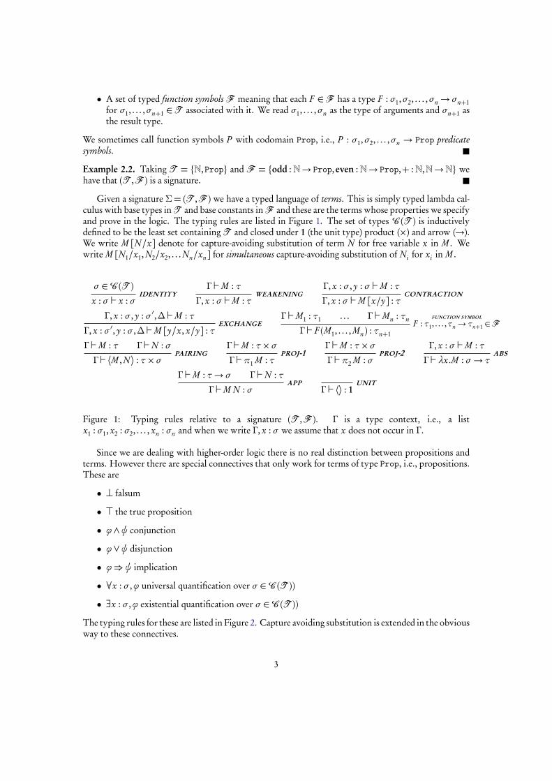
Given a signature Σ= (T ,F ) we have a typed language of terms. This is simply typed lambda cal-culus with base types in T and base constants inF and these are the terms whose properties we specifyand prove in the logic. The typing rules are listed in Figure 1. The set of types C (T ) is inductivelydefined to be the least set containing T and closed under 1 (the unit type) product (×) and arrow (→).We write M [N/x] denote for capture-avoiding substitution of term N for free variable x in M . Wewrite M [N1/x1,N2/x2, . . .Nn/xn] for simultaneous capture-avoiding substitution of Ni for xi in M .

σ ∈C (T )x : σ ` x : σ

IDENTITYΓ `M : τ

Γ , x : σ `M : τWEAKENING

Γ , x : σ , y : σ `M : τ

Γ , x : σ `M [x/y] : τCONTRACTION

Γ , x : σ , y : σ ′,∆ `M : τ

Γ , x : σ ′, y : σ ,∆ `M [y/x, x/y] : τEXCHANGE

Γ `M1 : τ1 . . . Γ `Mn : τn

Γ ` F (M1, . . . , Mn) : τn+1

FUNCTION SYMBOL

F : τ1, . . . ,τn → τn+1 ∈F

Γ `M : τ Γ `N : σ

Γ ` ⟨M ,N ⟩ : τ×σPAIRING

Γ `M : τ×σΓ `π1 M : τ

PROJ-1Γ `M : τ×σΓ `π2 M : σ

PROJ-2Γ , x : σ `M : τ

Γ ` λx.M : σ→ τABS

Γ `M : τ→ σ Γ `N : τ

Γ `M N : σAPP

Γ ` ⟨⟩ : 1UNIT

Figure 1: Typing rules relative to a signature (T ,F ). Γ is a type context, i.e., a listx1 : σ1, x2 : σ2, . . . , xn : σn and when we write Γ , x : σ we assume that x does not occur in Γ .

Since we are dealing with higher-order logic there is no real distinction between propositions andterms. However there are special connectives that only work for terms of type Prop, i.e., propositions.These are

• ⊥ falsum

• > the true proposition

• ϕ ∧ψ conjunction

• ϕ ∨ψ disjunction

• ϕ⇒ψ implication

• ∀x : σ ,ϕ universal quantification over σ ∈C (T ))

• ∃x : σ ,ϕ existential quantification over σ ∈C (T ))

The typing rules for these are listed in Figure 2. Capture avoiding substitution is extended in the obviousway to these connectives.

3

Γ `⊥ : PropFALSE

Γ `> : PropTRUE

Γ ` ϕ : Prop Γ `ψ : Prop

Γ ` ϕ ∧ψ : PropCONJ

Γ ` ϕ : Prop Γ `ψ : Prop

Γ ` ϕ ∨ψ : PropDISJ

Γ ` ϕ : Prop Γ `ψ : Prop

Γ ` ϕ⇒ψ : PropIMPL

Γ , x : σ ` ϕ : Prop

Γ ` ∀x : σ ,ϕ : PropFORALL

Γ , x : σ ` ϕ : Prop

Γ ` ∃x : σ ,ϕ : PropEXISTS

Figure 2: Typing rules for logical connectives. Note that these are not introduction and eliminationrules for connectives. These merely state that some things are propositions, i.e., of type Prop

Notice that we did not include an equality predicate. This is just for brevity. In higher-order logicequality can be defined as Leibniz equality, see, e.g., [Jac99]. (See the references in the introduction forhow equality can be modeled in hyperdoctrines using left adjoints to reindexing along diagonals.)

We can now describe sequents and provide basic rules of natural deduction. If ψ1,ψ2, . . . ,ψn havetype Prop in context Γ we write Γ ` ψ1,ψ2, . . . ,ψn and call Ξ = ψ1, . . . ,ψn the propositional context.Given Γ ` Ξ and Γ ` ϕ we have a new judgment Γ | Ξ ` ϕ. The rules for deriving these are listed inFigure 3.

3 A first set-theoretic modelWhat we have described up to now is a system for deriving two judgments, Γ `M : τ and Γ | Ξ ` ϕ. Wenow describe a first model where we give meaning to types, terms, propositions and sequents.

We interpret the logic in the category Set of sets and functions. There are several things to interpret.

• The signature (T ,F ).

• The types C (T )

• The terms of simply typed lambda calculus

• Logical connectives

• The sequent Γ | Ξ `ψ

Interpretation of the signature For a signature (T ,F ) we pick interpretations. That is, for eachτ ∈ T we pick a set Xτ but for Prop we pick the two-element set of “truth-values” 2= 0,1. For eachF : τ1,τ2, . . . ,τn→ τn+1 we pick a function f from Xτ1

×Xτ2× · · ·×Xτn

to Xτn+1.

Interpretation of simply typed lambda calculus Having interpreted the signature we extend theinterpretation to types and terms of simply typed lambda calculus. Each type τ ∈ C (T ) is assigned aset JτK by induction

JτK=Xτ if τ ∈ TJτ×σK= JτK× JσK

Jτ→ σK= JσKJτK

4

where on the right the operations are on sets, that is A×B denotes the cartesian product of sets and BA

denotes the set of all functions from A to B .Interpretation of terms proceeds in a similarly obvious way. We interpret the typing judgment

Γ ` M : τ. For such a judgment we define JΓ `M : τK as a function from JΓ K to JτK, where JΓ K =Jτ1K × Jτ2K × · · ·JτnK for Γ = x1 : τ1, x2 : τ2, . . . , xn : τn . The interpretation is defined as usual incartesian closed categories.

We then have the following result which holds for any cartesian closed category, in particular Set.

Proposition 3.1. The interpretation of terms validates all the β and η rules, i.e., if Γ ` M ≡ N : σ thenJΓ `M : σK= JΓ `N : σK.

The β and η rules are standard computation rules for simply typed lambda calculus. We do notwrite them here explicitly and do not prove this proposition since it is a standard result relating simplytyped lambda calculus and cartesian closed categories. But it is good exercise to try and prove it.

Exercise 3.1. Prove the proposition. Consider all the rules that generate the equality judgment ≡ andprove for each that it is validated by the model. ♦

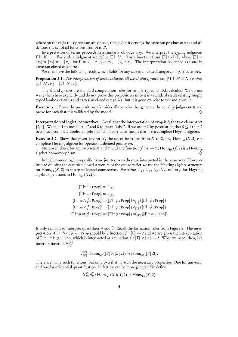
Interpretation of logical connectives Recall that the interpretation of Prop is 2, the two element set0,1. We take 1 to mean “true” and 0 to mean “false”. If we order 2 by postulating that 0 ≤ 1 then 2becomes a complete Boolean algebra which in particular means that it is a complete Heyting algebra.

Exercise 3.2. Show that given any set X , the set of functions from X to 2, i.e., HomSet (X , 2) is acomplete Heyting algebra for operations defined pointwise.

Moreover, check for any two sets X and Y and any function f : X → Y , HomSet ( f , 2) is a Heytingalgebra homomorphism. ♦

In higher-order logic propositions are just terms so they are interpreted in the same way. Howeverinstead of using the cartesian closed structure of the category Set we use the Heyting algebra structureon HomSet (X , 2) to interpret logical connectives. We write >X , ⊥X , ∧X , ∨X and ⇒X for Heytingalgebra operations in HomSet (X , 2).

JΓ `> : PropK=>JΓK

JΓ `⊥ : PropK=⊥JΓK

JΓ ` ϕ ∧ψ : PropK= (JΓ ` ϕ : PropK)∧JΓK (JΓ `ψ : PropK)

JΓ ` ϕ ∨ψ : PropK= (JΓ ` ϕ : PropK)∨JΓK (JΓ `ψ : PropK)

JΓ ` ϕ⇒ψ : PropK= (JΓ ` ϕ : PropK)⇒JΓK (JΓ `ψ : PropK)

It only remains to interpret quantifiers ∀ and ∃. Recall the formation rules from Figure 2. The inter-pretation of Γ ` ∀x : σ ,ϕ : Prop should be a function f : JΓ K→ 2 and we are given the interpretationof Γ , x : σ ` ϕ : Prop, which is interpreted as a function g : JΓ K× JσK→ 2. What we need, then, is afunction function ∀JσK

JΓK

∀JσKJΓK : HomSet (JΓ K× JσK , 2)→HomSet (JΓ K , 2) .

There are many such functions, but only two that have all the necessary properties. One for universaland one for existential quantification. In fact we can be more general. We define

∀YX ,∃Y

X : HomSet (X ×Y, 2)→HomSet (X , 2)

5

for any sets X and Y and ϕ : X ×Y → 2 as

∀YX (ϕ) = λx.

¨

1 if ∀y ∈ Y,ϕ(x, y) = 10 otherwise

= λx.

¨

1 if x×Y ⊆ ϕ−1 [1]0 otherwise

∃YX (ϕ) = λx.

¨

1 if ∃y ∈ Y,ϕ(x, y) = 10 otherwise

= λx.

¨

1 if x×Y ∩ϕ−1 [1] 6= ;0 otherwise

To understand these definitions and to present them graphically a presentation of functions fromX → 2 as subsets of X is useful. Consider the problem of obtaining a subset of X given a subset of X×Y .One natural way to do this is to “project out” the second component, i.e., map a subset A⊆ X ×Y toπ [A] = π(z) | z ∈A where π : X × Y → X is the first projection. Observe that this gives rise to∃Y

X . Geometrically, if we draw X on the horizontal axis and Y on the vertical axis, A is a region on thegraph. The image π [A] includes all x ∈ X such that the vertical line at x intersects A in at least onepoint.

We could instead choose to include only points x ∈ X such that the vertical line at x is a subset ofA. This way, we would get exactly ∀Y

X (A).To further see that these are not arbitrary definitions but in fact essentially unique show the follow-

ing.

Exercise 3.3. Let π∗X ,Y = HomSet (π, 2) : HomSet (X , 2)→ HomSet (X ×Y, 2). Show that ∀YX and ∃Y

Xare monotone functions (i.e., functors) and that ∀Y

X is the right adjoint to π∗X ,Y and ∃YX its left adjoint.

Concretely the last part means to show for any ϕ : X → 2 and ψ : X ×Y → 2 that

π∗X ,Y (ϕ)≤ψ ⇐⇒ ϕ ≤∀YX (ψ)

and

∃YX (ψ)≤ ϕ ⇐⇒ ψ≤π∗X ,Y (ϕ).

♦Moreover, ∀Y

X and ∃YX have essentially the same definition for all X , i.e., they are natural in X . This

is expressed as the commutativity of the diagram

HomSet (X′×Y, 2) HomSet (X ×Y, 2)

HomSet (X′, 2) HomSet (X , 2)

∀YX ′

HomSet(s×idY ,2)

∀YX

HomSet(s ,2)

for any s : X →X ′ (remember that the functor HomSet (−, 2) is contravariant) and analogously for ∃.This requirement that ∀Y

X and ∃YX are “natural” is often called the Beck-Chevalley condition.

Exercise 3.4. Show that ∃YX and ∀Y

X are natural in X . ♦Using these adjoints we can finish the interpretation of propostions:

JΓ ` ∀x : σ ,ϕ : PropK= ∀JσKJΓK (JΓ , x : σ ` ϕ : PropK)

JΓ ` ∃x : σ ,ϕ : PropK= ∃JσKJΓK (JΓ , x : σ ` ϕ : PropK)

Given a sequence of terms ~M = M1, M2, . . . , Mn of type ~σ = σ1,σ2, . . . ,σn in context Γ we definerΓ ` ~M : ~σ

zas the tupling of interpretations of individual terms.

6

Exercise 3.5. Show that given contexts Γ = y1 : σ1, . . . , ym : σm and∆= x1 : δ1, . . . , xn : δn we have thefollowing property of the interpretation for any N of type τ in context ∆ and any sequence of terms~M of appropriate types

rΓ `N

~M/~x

: τz= J∆ `N : τK

rΓ ` ~M : ~δ

z

To show this proceed by induction on the typing derivation for N . You will need to use the naturalityof quantifiers. ♦

Remark 3.2. If you have done Exercise 3.5, you will have noticed that the perhaps mysterious Beck-Chevalley condition is nothing but the requirement that the model respects substitution, i.e., that theinterpretation of

(∀y : σ ,ϕ) [M/x]

is equal to the interpretation of

∀y : σ , (ϕ [M/x])

for x 6= y.

4 HyperdoctrineUsing the motivating example above we now define the concept of a hyperdoctrine, which will be ourgeneral notion of a model of higher-order logic for which we prove soundness of the interpretationdefined above.

Definition 4.1. A hyperdoctrine is a cartesian closed categoryC together with an object Ω ∈C (calledthe generic object) and for each object X ∈ C a choice of a partial order on the set HomC (X ,Ω) suchthat the conditions below hold. We writeP for the contravariant functor HomC (−,Ω).

• P restricts to a contravariant functorC op→Heyt, fromC to the category of Heyting algebrasand Heyting algebra homomorphisms, i.e., for each X , P (X ) is a Heyting algebra and for eachf ,P ( f ) is a Heyting algebra homomorphisms, in particular it is monotone.

• For any objects X ,Y ∈ C and the projection π : X × Y → X there exist monotone functions1

∃YX and ∀Y

X such that ∃YX is a left adjoint to P (π) : P (X ) → P (X × Y ) and ∀Y

X is its rightadjoint. Moreover, these adjoints are natural in X , meaning that for any morphism s : X → X ′

the diagrams

P (X ′×Y ) P (X ×Y )

P (X ′) P (X )

∀YX ′

P (s×idY )

∀YX

P (s)

P (X ′×Y ) P (X ×Y )

P (X ′) P (X )

∃YX ′

P (s×idY )

∃YX

P (s)

commute.

This naturality requirement is called the Beck-Chevalley condition.

1We do not require them to be Heyting algebra homomorphisms.

7

Example 4.2. The category Set together with the object 2 for the generic object which we described inSection 3 is a hyperdoctrine. See the discussion and exercises in Section 3 for the definitions of adjoints.

4.1 Interpretation of higher-order logic in a hyperdoctrineThe interpretation of higher-order logic in a general hyperdoctrine proceeds much the same as the in-terpretation in Section 3.

First, we choose objects of C for base types and morphisms for function symbols. We must, ofcourse, choose the interpretation of the type Prop to be Ω.

We then interpret the terms of simply typed lambda calculus using the cartesian closed structure ofC and the logical connectives using the fact that each hom-set is a Heyting algebra. The interpretationis spelled out in Figure 4.

Note that the interpretation itself requires no properties of the adjoints to P (π). However, toshow that the interpretation is sound, i.e., that it validates all the rules in Figure 3, all the requirementsin the definition of a hyperdoctrine are essential. A crucial property of the interpretation is that it mapssubstitution into composition in the following sense.

Proposition 4.3. Let ~M = M1, M2, . . . Mn be a sequence of terms and Γ a context such that for all i ∈1,2, . . . , n, Γ `Mi : δi . Let ∆ = x1 : δ1, x2 : δ2, . . . , xn : δn be a context and N be a term such that∆ `N : τ. Then the following equality holds

rΓ `N

~M/~x

: τz= J∆ `N : τK

rΓ ` ~M : ~δ

z(2)

whererΓ ` ~M : ~δ

z= ⟨JΓ `Mi : δiK⟩

ni=1 .

Further, if N is of type Prop, i.e., if τ = Prop thenrΓ `N

~M/~x

: Propz=P

rΓ ` ~M : ~δ

z(J∆ `N : PropK) (3)

Proof. Only the proof of the first equality requires work since if we know that substitution is mappedto composition then the second equality is just the first equality hidden by using theP functor since itacts on morphisms by precomposition.

To prove (2) we proceed by induction on the derivation of ∆ `N : τ. All of the cases are straight-forward. We only show some of them to illustrate key points. To remove the clutter we omit explicitcontexts and types, i.e., we write JNK instead of J∆ `N : τK.

• When N = K L and ∆ `K : σ→ τ and ∆ ` L : σ . Recall that substitution distributes over appli-cation and that we can use the induction hypothesis for K and L. We have

r(K L)

~M/~xz=

r

K

~M/~x

L

~M/~x

z

= ε Dr

K

~M/~xz

,r

L

~M/~xzE

which by induction is equal to

= ε D

JKK r~Mz

,JLK r~MzE

8

which by a simple property of products gives us

= ε ⟨JKK ,JLK⟩ r~Mz

= JK LK r~Mz

• When N = λx.K and∆, x : σ `K : τwe first use the fact that when Γ `Mi : δi then Γ , y : σ `Mi : δi

by a single application of weakening and we write π∗( ~M ) for ~M in this extended context. So wehave

r(λx.K)

~M/~xz=

rλy.K

π∗

~M

/~x, y/x

z

=Λr

K

π∗

~M

/~x, y/x

z

=Λ

JKK rπ∗

~M

, yz

induction hypothesis for ~M , y

and since the interpretation no weakening is precomposition with the projection we have

=Λ

JKK Dr

~Mzπ,π′

E

which by a simple property of products gives us

=Λ

JKK r~Mz× idJσK

which by a simple property of exponential transposes finally gives us

=Λ (JKK) r~Mz= JNK

r~Mz

.

Admittedly we are a bit sloppy with the bound variable x but to be more precise we would haveto define simultaneous subsitution precisely which is out of scope of this tutorial and we have notskipped anything essential.

• When N = ϕ ∧ψ we haver(ϕ ∧ψ)

~M/~xz=

r

ϕ

~M/~x

∧

ψ

~M/~x

z

=rϕ

~M/~xz∧

rψ

~M/~xz

which by the induction hypothesis and the definition ofP gives us

= JϕK r~Mz∧ JψK

r~Mz

=Pr~Mz(JϕK)∧P

r~Mz(JψK)

and since by definitionP is a Heyting algebra homomorphism it commutes with ∧ giving us

=Pr~Mz(JϕK∧ JψK)

9

and again using the definition ofP but in the other direction

= (JϕK∧ JψK) r~Mz

= Jϕ ∧ψK r~Mz

which is conveniently exactly what we want. All the other binary connectives proceed in exactlythe same way; use the fact thatP is a Heyting algebra homomorphism.

• When N = ∀x : σ ,ϕ we haver(∀x : σ ,ϕ)

~M/~xz=

r∀y : σ ,

ϕ

~π∗(M )/~x, y/x

z

the definition of the interpretation of ∀ gives us

= ∀rϕ

π∗( ~M )/~x, y/xz

where we use π∗ for the same purpose as in the case for λ-abstraction. The induction hypothesisfor ϕ now gives us

= ∀

JϕK rπ∗( ~M ), y

z

and by the same reasoning as in the λ-abstraction case we get

= ∀

JϕK r~Mz× idJσK

.

Using the definition ofP we have

= ∀

Pr~Mz× idJσK

(JϕK)

.

Now we are in a situation where we can use the Beck-Chevalley condition to get

=Pr~Mz(∀ (JϕK))

which by the same reasoning as in the last step of the previous case gives us

= ∀ (JϕK) r~Mz

= J∀x : σ ,ϕK r~Mz

.

These four cases cover the essential ideas in the proof. The other cases are all essentially the same as oneof the four cases covered.

Theorem 4.4 (Soundness). Let Θ = ϑ1,ϑ2, . . . ,ϑn be a propositional context. If Γ | Θ ` ϕ is derivableusing the rules in Figure 3 then

n∧

i=1

JΓ ` ϑi : PropK≤ JΓ ` ϕ : PropK

in the Heyting algebraP (JΓ K).In particular if Γ | − ` ϕ is derivable then JΓ ` ϕ : PropK=>.

10

Proof. The proof is, of course, by induction on the derivation Γ | Θ ` ϕ. Most of the cases are straight-forward. We only show the cases for the universal quantifier where we also use Proposition 4.3. In theproof we again omit explicit contexts to avoid clutter.

First, the introduction rule. We assume that the claim holds for Γ , x : σ | Θ ` ϕ and show that it alsoholds for Γ | Θ ` ∀x : σ ,ϕ.

By definition

J∀x : σ ,ϕK= ∀JσKJΓK (JϕK)

and thus we need to shown∧

i=1

JΓ ` ϑi : PropK≤∀JσKJΓK (JϕK) .

Since by definition ∀ is the right adjoint toP (π) this is equivalent to

P (π) n∧

i=1

JΓ ` ϑi : PropK

≤ JϕK

whereπ : JΓ K×JσK→ JΓ K is of course the first projection. We cannot do much with the right side, so letus simplify the left-hand side. By definitionP (π) is a Heyting algebra homomorphism so in particularit commutes with conjuction which gives us

P (π) n∧

i=1

JΓ ` ϑi : PropK

=n∧

i=1

P (π) (JΓ ` ϑi : PropK)

using the definition ofP we get

=n∧

i=1

JΓ ` ϑi : PropK π.

Now recall the definition of the interpretation of terms, in particular the definition of the interpretationof weakening in Figure 4. It gives us that

JΓ ` ϑi : PropK π= JΓ , x : σ ` ϑi : PropK .

so we get

n∧

i=1

JΓ ` ϑi : PropK π=n∧

i=1

JΓ , x : σ ` ϑi : PropK

By the induction hypothesis we have

n∧

i=1

JΓ , x : σ ` ϑi : PropK≤ JϕK

which concludes the proof of the introduction rule for ∀.

Exercise 4.1. Where did we use the side-condition that x does not appear in Θ? ♦

11

For the elimination rule assume that Γ `M : σ and that the claim holds for Γ | Θ ` ∀x : σ ,ϕ. Weneed to show it for Γ | Θ ` ϕ [M/x], so we need to show

n∧

i=1

JΓ ` ϑi : PropK≤ JΓ ` ϕ [M/x] : PropK

From Proposition 4.3 (the second equality) we have

JΓ ` ϕ [M/x] : PropK=P¬

idJΓK,JΓ `M : σK¶

(JΓ , x : σ ` ϕ : PropK) . (4)

SinceP (π) is left adjoint to ∀JσKJΓK we have in particular that

P (π) ∀JσKJΓK ≤ idP (JΓ ,x:σK)

which is the counit of the adjunction. Thus

JΓ , x : σ ` ϕ : PropK≥

P (π) ∀JσKJΓK

(JΓ , x : σ ` ϕ : PropK)

whose right-hand side is, by definition of the interpretation of the universal quantifier, equal to

=P (π) (JΓ ` ∀x : σ ,ϕ : PropK) ,

which by induction hypothesis and monotonicity ofP (π) is greater than

≥P (π) n∧

i=1

JΓ ` ϑi : PropK

.

Further, sinceP is a contravariant functor we have

P¬

idJΓK,JΓ `M : σK¶

P (π) =P

π ¬

idJΓK,JΓ `M : σK¶

=P

idJΓK

.

Thus combining the last two results with (4) we have

JΓ ` ϕ [M/x] : PropK≥P

idJΓK

n∧

i=1

JΓ ` ϑi : PropK

=n∧

i=1

JΓ ` ϑi : PropK

concluding the proof.

4.2 A class of Set-based hyperdoctrinesTo get other examples of Set-based hyperdoctrines, we can keep the base category Set and replace thegeneric object 2 with a different complete Heyting algebra.

Definition 4.5. A complete Heyting algebra is a Heyting algebra that is complete as a lattice.

Exercise 4.2. Show that any complete Heyting algebra satisfies the infinite distributivity law

x ∧∨

i∈I

yi =∨

i∈I

(x ∧ yi )

Hint: use your category theory lessons (left adjoints preserve. . . ). ♦

12

Exercise 4.3. Show that if H is a (complete) Heyting algebra and X any set then the set of all functionsfrom X to (the underlying set of) H when ordered pointwise, i.e., ϕ ≤H X ψ ⇐⇒ ∀x ∈ X ,ϕ(x) ≤Hψ(x), is a (complete) Heyting algebra with operations also inherited pointwise from H , e.g. (ϕ ∧H X

ψ)(x) = ϕ(x)∧H ψ(x). ♦

Theorem 4.6. Let H be a complete Heyting algebra. Then Set together with the functor HomSet (−, H )and the generic object H is a hyperdoctrine.

Proof. Clearly Set is a cartesian closed category and from Exercise 4.3 we know that HomSet (X , H ) is acomplete Heyting algebra. To show that HomSet (−, H ) is a functor into Heyt we need to establish thatfor any function f , HomSet ( f , H ) is a Heyting algebra homomorphism. We use greek letters ϕ,ψ, . . .for elements of HomSet (X , H ).

Recall that the action of the hom-functor on morphisms is by precomposition: HomSet ( f , H ) (ϕ) =ϕ f . We now show that for any f : Y →X , HomSet ( f , H ) preserves conjunction and leave the otheroperations as an exercise since the proof is essentially the same. Let ϕ,ψ ∈ HomSet (X , H ) and y ∈ Ythen

HomSet ( f , H ) (ϕ ∧H X ψ)(y) = ((ϕ ∧H X ψ) f )(y) = ϕ( f (y))∧H ψ( f (y)) = ((ϕ f )∧H Y (ψ f ))(y).

As y was arbitrary we have HomSet ( f , H ) (ϕ ∧H X ψ) = (ϕ f )∧H Y (ψ f ), as needed.Observe that we have not yet used completeness of H anywhere. We need completeness to define

adjoints ∀YX and ∃Y

X to HomSet (π, H ) for π : X ×Y →X which we do now.To understand the definitions of adjunctions recall that universal quantification is akin to an infinite

conjunction and existential quantification is akin to infinite disjunction. Let X and Y be sets and ϕ ∈HomSet (X ×Y, H ). Define

∃YX (ϕ) = λx.

∨

y∈Y

ϕ(x, y)

∀YX (ϕ) = λx.

∧

y∈Y

ϕ(x, y).

It is a straightforward exercise to show that ∃YX and ∀Y

X are monotone. We now show that ∃YX is left

adjoint to HomSet (π, H ) and leave the proof that ∀YX is right adjoint as another exercise. We show the

two implications separately.Let ϕ ∈ HomSet (X ×Y, H ) and ψ ∈ HomSet (X , H ). Assume that ∃Y

X (ϕ) ≤ ψ. We are to showϕ ≤ HomSet (π, H ) (ψ) which reduces to showing for any x ∈ X and y ∈ Y that ϕ(x, y) ≤ ψ(π(x, y))which further reduces to showing ϕ(x, y)≤ψ(x).

Let x ∈ X and y ∈ Y . By assumption ∃YX (ϕ)(x) ≤ ψ(x) which simplifies to

∨

y∈Y ϕ(x, y) ≤ ψ(x).By definition of supremum ϕ(x, y)≤

∨

y∈Y ϕ(x, y) so we get ϕ(x, y)≤ψ(x) by transitivity.Note that for this direction we only needed that

∨

y∈Y ϕ(x, y) is an upper bound of the set ϕ(x, y) | y ∈ Y ,not that it is the least upper bound. We need this last property for the other direction.

For the other direction let again ϕ ∈ HomSet (X ×Y, H ) and ψ ∈ HomSet (X , H ). Assume thatϕ ≤HomSet (π,ψ). We are to show ∃Y

X (ϕ)≤ψwhich reduces to showing for any x ∈X ,∨

y∈Y ϕ(x, y)≤ψ(x). Let x ∈ X . The assumption ϕ ≤ HomSet (π,ψ) gives us that for any y ∈ Y , ϕ(x, y) ≤ ψ(x)which means that ψ(x) is the upper bound of the set ϕ(x, y) | y ∈ Y . But by definition of supremum,∨

y∈Y ϕ(x, y) is the least upper bound, so∨

y∈Y ϕ(x, y)≤ψ(x).

Exercise 4.4. Show that ∀YX is the right adjoint to HomSet (π, H ). ♦

13

What we are still missing is the Beck-Chevalley condition for ∃YX and ∀Y

X . Again, we show this for∃Y

X and leave the other as an exercise for the reader.Let X and X ′ be sets and s : X → X ′ a function. We need to show that ∃Y

X HomSet (s × idY , H ) =HomSet (s , H ) ∃Y

X ′ . Let ϕ ∈HomSet (X′×Y, H ). Then

∃YX HomSet (s × idY , H )

(ϕ) = ∃YX (ϕ (s × idY )) = λx.

∨

y∈Y

ϕ(s(x), y)

and

HomSet (s , H ) ∃YX ′

(ϕ) = ∃YX ′(ϕ) s .

For any x ∈X ′ we have

∃YX ′(ϕ) s

(x) = ∃YX ′(ϕ)(s(x)) =

∨

y∈Y

ϕ(s(x), y)

which means ∃YX ′(ϕ) s = λx.

∨

y∈Y ϕ(s(x), y), which is exactly what we need it to be.

Exercise 4.5. Show that the Beck-Chevalley condition also holds for ∀YX . ♦

We now give some examples of complete Heyting algebras. We only give definitions and leave thestraightforward verifications of the axioms as an exercise

Exercise 4.6. Let P be a preordered set (i.e., a set with a reflexive and transitive relation ≤). Show thatthe set of upwards closed subsets of P ,P ↑ (P )

P ↑ (P ) = A⊆ P | ∀x ∈A,∀y ∈ P, x ≤ y⇒ y ∈A

is a complete Heyting algebra for the following operations

>= P ⊥= ; A∨B =A∪B A∧B =A∩B∨

i∈I

Ai =⋃

i∈I

Ai

∧

i∈I

Ai =⋂

i∈I

Ai A⇒ B = x ∈ P | ∀y ≥ x, y ∈A⇒ y ∈ B

Concretely show that all these operations are well defined (that the sets defined are again upwards closed)and that they satisfy the axioms of a complete Heyting algebra.

Also show that the set of downwards closed subsets of P ,P ↓ (P ) is a complete Heyting algebra (youonly need to change the definition of one of the operations). ♦

4.3 Examples based on monoidsAnother set of examples is useful in modeling various logics dealing with resources. We need somedefinitions.

Definition 4.7. Let f , g : A* B be two partial functions and a ∈ A. We write f (a)' g (a) for Kleeneequality meaning that if either of the sides is defined then both are and they are equal.

Definition 4.8. A partial commutative monoid M is a set M together with a partial function · : M ×M *M(multiplication) and an element 1 ∈M (the unit) such that the following axioms hold:

• for all m ∈M , m · 1' 1 ·m ' m (in particular 1 ·m and m · 1 are always defined)

14

• for m, n ∈M , m · n ' n ·m (commutativity)

• for `, m, n ∈M , ` · (m · n)' (` ·m) · n.

We write a#b to say that a · b is defined.

Example 4.9. Let H be the set of finite partial maps from N to X where X is some set. It could forinstance be the set of values of some programming language. ThenH would be a model of the heap.

Define the operation · :H×H*H as follows

f · g =¨

f ] g if dom ( f )∩dom (g ) = ;undefined otherwise

where

( f ] g )(x) =

f (x) x ∈ dom ( f )g (x) x ∈ dom (g )undefined otherwise

Then it is easy to see thatHwith · is a partial commutative monoid. Its unit is the (unique) functionwith the empty domain, i.e., the everywhere undefined partial function.

Given a partial commutative monoid M there is a canonical preorder associated with it that arisesfrom multiplication ·. It is called the extension order. Concretely, we define

m ≤ n ⇐⇒ ∃k ∈M , m · k ' n

(note that associativity of · is used to show that ≤ is transitive).

Example 4.10. For the example partial commutative monoidH above the extension order can equiva-lently be defined as

f ≤ g ⇐⇒ dom ( f )⊆ dom (g )∧∀x ∈ dom ( f ) , f (x)' g (x)

If we think of f and g as heaps then f ≤ g if the heap g is derived from f by allocating some newlocations.

As we have seen in Exercise 4.6 given a preordered set P , the set of upwards closed subsets of P is acomplete Heyting algebra. It turns out that given a partial commutative monoid and its derived preorderwe can lift the multiplication of the monoid to multiplication of upwards closed subsets, giving rise toa (complete) BI-algebra.

Definition 4.11. A (complete) BI-algebra H is a (complete) Heyting algebra with an additional constantI and two binary operations ? and→? such that the following axioms hold

• ? is monotone: for any h, h ′, g , g ′, if h ≤ h ′ and g ≤ g ′ then h ? g ≤ h ′ ? g ′.

• I is the unit for ?.

• ? is commutative and associative

• for any h, h ′, h ′′ ∈H , h ? h ′ ≤ h ′′ ⇐⇒ h ≤ h ′→?h ′′ (→? is right adjoint to ?).

15

Note in contrast to the operations of a (complete) Heyting algebra, which are uniquely determinedby the order relation (why?), there can be (potentially) many different definitions of ?,→? and I (although→? is determined by ?).

Exercise 4.7. Any (complete) Heyting algebra is trivially a (complete) BI algebra. What can we choosefor operations ?, I and→?? ♦

Exercise 4.8. Show that if H is a (complete) BI-algebra and X is any set, then the set of functions fromX to H is another (complete) BI-algebra with operations defined pointwise. ♦

Of course, we want nontrivial examples. Partial commutative monoids give rise to such.

Example 4.12. Let M be a partial commutative monoid. Then the set of upwards closed subsets of M(with respect to the extension order) is a complete BI-algebra.

We already know that it is a complete Heyting algebra. We need to define I , ? and→?. The operation? is a pointwise lifting of the operation · of the monoid in the sense

A?B = m · n | m ∈A, n ∈ B , m · n defined .

The unit I is the whole monoid M .Recalling that the order on P ↑ (M ) is subset inclusion it is clear that ? is monotone. To see that M

is the unit for ? we prove two inclusions. Let A∈P ↑ (M ). We wish to show A?M =A.Suppose m ∈ A. Since 1 ∈ M and m · 1 ' m clearly, m ∈ A?M . Conversely, suppose m ∈ A?M .

By definition there exists a ∈A and n ∈M , such that m ' a · n. This means (recall the definition of theextension order) that m ≥ a. Since A is upwards closed by definition and a ∈ A, it must be that m ∈ Aas well.

Showing M ?A= A is analogous. The fact that it is commutative and associative likewise followseasily.

Exercise 4.9. Show that ? is commutative and associative. ♦

Finally, the operation→? is defined as

A→?B = m ∈M | ∀a ∈A,a#m⇒ m · a ∈ B

Or more explicitly

Exercise 4.10. Show that A→?B is well defined (i.e., upwards closed) and that it is the right adjoint to ?.The latter means more precisely that for any A, the mapping B 7→A→?B is right adjoint to the mappingC 7→A?C . ♦

4.4 BI-hyperdoctrinesDefinition 4.13. A BI-hyperdoctrine is a hyperdoctrine (C ,Ω) such that P restricts to a functor intothe category of BI-algebras and BI-algebra homomorphisms.

Example 4.14. Let H be a complete BI-algebra. Then Set together with the hom-functor HomSet (−, H )is a BI-hyperdoctrine.

Since a complete BI-algebra is in particular a complete Heyting algebra, we know that the hom-functor forms a hyperdoctrine. From Exercise 4.8 we know that for each X , HomSet (X , H ) is a BI-algebra. It remains to show that for any function f , HomSet ( f , H ) is a BI-algebra homomorphism.This is straightforward and we leave it as an exercise for the reader.

16

BI-hyperdoctrines can be used to model higher-order separation logic. See [BBTS07] for details ofhow this is done.

A canonical example of a BI-hyperdoctrine is the hyperdoctrine arising from the partial commuta-tive monoid of heaps from Example 4.9. Predicates are modeled as upwards closed sets of heaps andobserve that for predicates P and Q the predicate P ?Q contains those heaps that can be split into twodisjoint heaps; a heap satisfying P and a heap satisfying Q.

More generally, we can take a partial commutative monoid that represents abstract resources andbuild a model of higher-order separation logic. Then for predicates P and Q the predicate P ?Q willcontain resources which can be split into resources satisfying P and resources satisfying Q. But theseparation does not have to be as literal as with heaps, that is, the splitting does not have to representactual splitting of the heap but only some fiction of separation, depending on what the monoid ofresources is.

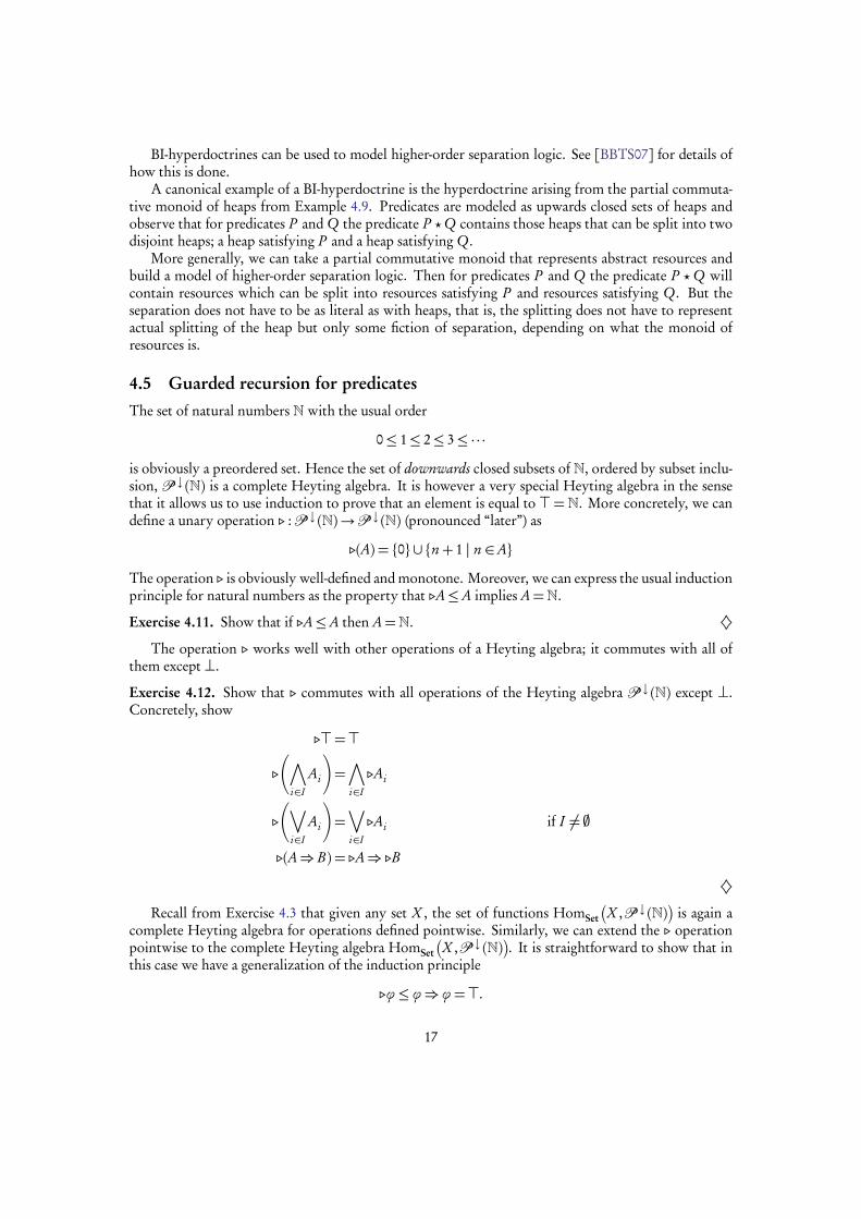
4.5 Guarded recursion for predicatesThe set of natural numbers N with the usual order

0≤ 1≤ 2≤ 3≤ · · ·

is obviously a preordered set. Hence the set of downwards closed subsets of N, ordered by subset inclu-sion, P ↓ (N) is a complete Heyting algebra. It is however a very special Heyting algebra in the sensethat it allows us to use induction to prove that an element is equal to > = N. More concretely, we candefine a unary operation . :P ↓ (N)→P ↓ (N) (pronounced “later”) as

.(A) = 0 ∪ n+ 1 | n ∈A

The operation . is obviously well-defined and monotone. Moreover, we can express the usual inductionprinciple for natural numbers as the property that .A≤A implies A=N.

Exercise 4.11. Show that if .A≤A then A=N. ♦

The operation . works well with other operations of a Heyting algebra; it commutes with all ofthem except ⊥.

Exercise 4.12. Show that . commutes with all operations of the Heyting algebra P ↓ (N) except ⊥.Concretely, show

.>=>

.

∧

i∈I

Ai

=∧

i∈I

.Ai

.

∨

i∈I

Ai

=∨

i∈I

.Ai if I 6= ;

.(A⇒ B) = .A⇒ .B

♦

Recall from Exercise 4.3 that given any set X , the set of functions HomSet

X ,P ↓ (N)

is again acomplete Heyting algebra for operations defined pointwise. Similarly, we can extend the . operationpointwise to the complete Heyting algebra HomSet

X ,P ↓ (N)

. It is straightforward to show that inthis case we have a generalization of the induction principle

.ϕ ≤ ϕ⇒ ϕ =>.

17

Exercise 4.13. Show that if .ϕ ≤ ϕ then ϕ is the top element of HomSet

X ,P ↓ (N)

.Moreover, show that . on HomSet

X ,P ↓ (N)

also commutes with the same Heyting algebra oper-ations as . onP ↓ (N).

Finally, show that if f : X → Y is any function then for any ϕ ∈HomSet

Y,P ↓ (N)

we have

.

HomSet

f ,P ↓ (N)

(ϕ)

=HomSet

f ,P ↓ (N)

(.(ϕ))

which means that all the Heyting algebra morphisms HomSet

f ,P ↓ (N)

also preserve the operation.. ♦

All of these are straightforward to show directly from the definitions of all the operations but it isgood practice to show some of them to get used to the definitions.

The reason for introducing the . operation is that we can use it to show existence of certain guardedrecursively defined predicates. To show this, we need some auxiliary definitions. Until the end of thissection we are working in some complete Heyting algebra H =HomSet

X ,P ↓ (N)

for some set X .

Definition 4.15. Let ϕ,ψ ∈H . For n ∈N we define bϕcn ∈H as

bϕcn (x) = k ∈ ϕ(x) | k < n

and we write ϕ n=ψ for

bϕcn = bψcn .

Note that for any ψ,ϕ ∈ H we have ϕ 0=ψ and that ϕ n+1= ψ⇒ ϕn=ψ and finally that if ∀n,ϕ n=ψ then

ψ= ϕ.We say that a function Φ : H →H is non-expansive if for any ϕ,ψ ∈H and any n ∈N we have

ϕn=ψ⇒ Φ(ϕ) n=Φ(ψ)

and we say that it is contractive if for any ϕ,ψ ∈H and any n ∈N we have

ϕn=ψ⇒ Φ(ϕ) n+1= Φ(ψ).

We can now put . to good use.

Exercise 4.14. Show that . is contractive. Show that composition (either way) of a contractive andnon-expansive function is contractive. Conclude that if Φ is a non-expansive function on H then Φ .and . Φ are contractive. ♦

Finally the property we were looking for.

Proposition 4.16. If Φ : H → H is a contractive function then it has a unique fixed point, i.e., there is aunique ϕ ∈H such that Φ(ϕ) = ϕ.

We will prove a more general theorem later (Theorem 5.10) so we skip the proof at this point.However, uniqueness is easy to show and is a good exercise.

Exercise 4.15. Show that if Φ : H →H is contractive then the fixed point (if it exists) must necessarilybe unique.

Hint: Use contractiveness of Φ together with the fact that if bϕcn = bψcn for all n ∈ N then ϕ =ψ. ♦

18

4.5.1 Application to the logic

Suppose that we extend the basic higher-order logic with an operation . on propositions. Concretely,we add the typing judgment

Γ ` ϕ : Prop

Γ ` .ϕ : Prop

together with the following introduction and elimination rules

Γ | Ξ ` ϕΓ | Ξ ` .ϕ

MONOΓ | Ξ,.ϕ ` ϕΓ | Ξ ` ϕ

LÖB

We can interpret this extended logic in the hyperdoctrine arising from the complete Heyting algebraP ↓ (N) by extending the basic interpretation with

JΓ ` .ϕ : PropK= . (JΓ ` ϕ : PropK) .

The properties of . from Exercise 4.13 then give us the following properties of the logic.Judgments

Γ | Ξ ` .(ϕ ∧ψ)Γ | Ξ ` .ϕ ∧ .ψ

Γ | Ξ ` .ϕ ∧ .ψΓ | Ξ ` .(ϕ ∧ψ)

and if σ is inhabited, that is if there exists a term M such that −`M : σ then

Γ | Ξ ` .(∃x : σ ,ϕ)Γ | Ξ ` ∃x : σ ,.(ϕ)

Γ | Ξ ` ∃x : σ ,.(ϕ)Γ | Ξ ` .(∃x : σ ,ϕ)

and similar rules for all the other connectives except ⊥ are all valid in the model.Moreover, the property that for any function f , HomSet

f ,P ↓ (N)

preserves . gives us that therules

Γ | Ξ ` . (ϕ [N/x])Γ | Ξ ` (.ϕ) [N/x]

Γ | Ξ ` (.ϕ) [N/x]Γ | Ξ ` . (ϕ [N/x])

are valid, i.e., that . commutes with substitution. This is a property that must hold for the connectiveto be useful since we use substitution constantly in reasoning, most of the time implicitly. For instanceevery time we instantiate a universally quantified formula or when we prove an existential, we usesubstitution.

Exercise 4.16. Show that the rules we listed are valid. ♦

Finally, we would like show that we have fixed points of guarded recursively defined predicates.More precisely, suppose the typing judgment Γ , p : Propτ ` ϕ : Propτ is valid and that p inϕ only occursunder a . (or not at all). Then we would like there to exist a unique termµp.ϕ of type Propτ in contextΓ , i.e.,

Γ `µp.ϕ : Propτ

such that the following sequents hold

Γ , x : τ | (ϕ [µp.ϕ/p]) x ` (µp.ϕ) x Γ | (µp.ϕ) x ` (ϕ [µp.ϕ/p]) x. (5)

19

Observe that this implies

Γ | − ` ∀x : τ, (ϕ [µp.ϕ/p]) x⇔ (µp.ϕ) x

Recall that when interpreting higher-order logic in the hyperdoctrine HomSet

−,P ↓ (N)

the term ϕis interpreted as

JΓ , p : Propτ ` ϕ : PropτK : JΓ K×H →H

where H = JτK→ JPropK = JτK→P ↓ (N). Suppose that for each γ ∈ JΓ K the function Φγ : H → Hdefined as

Φγ (h) = JΓ , p : Propτ ` ϕ : PropτK (γ , h)

were contractive. Then we could appeal to Proposition 4.16 applied to Φγ so that for each γ ∈ Γ wewould get a unique element hγ ∈H , such that Φγ (h) = hγ , or, in other words, we would get a functionfrom Γ to H , mapping γ to hγ . Define

JΓ `µp.ϕ : PropτK

to be this function. We then have

JΓ `µp.ϕ : PropτK= hγ = JΓ , p : Propτ ` ϕ : PropτK (γ , hγ )

= JΓ , p : Propτ ` ϕ : PropτK (γ ,JΓ `µp.ϕ : PropτK)= JΓ ` ϕ [µp.ϕ/p] : PropτK

The last equality following from Proposition 4.3. Observe that this is exactly what we need to validatethe rules (5).

However not all interpretations where the free variable p appears under a .will be contractive. Thereason for this is that can choose interpretations of base constants from the signature to be arbitrarilybad and a single use of .will not make these non-expansive. The problem comes from the fact that we areusing a Set-based hyperdoctrine and so interpretations of terms (including basic function symbols) canbe any functions. If we instead used a category where we had a meaningful notion of non-expansivenessand contractiveness and all morphisms would be non-expansive by definition, then perhaps every termwith a free variable p guarded by a . would be contractive and thus define a fixed point.

Example 4.17. Consider a signature with a single function symbol of type F : Prop→ Prop and theinterpretation in the hyperdoctrine HomSet

−,P ↓ (N)

where we choose to interpret F as

JF K= λA.

¨

.(A) if A 6=N; if A=N

Exercise 4.17. Show that JF K is not non-expansive and that JF K. and .JF K are also not non-expansive.Show also that JF K . and . JF K have no fixed-points. ♦

This example (together with the exercise) shows that even though p appears under a . in

p : Prop ` F (.(p)) : Prop

the interpretation of p : Prop ` F (.(p)) : Prop has no fixed points and so we are not justified in addingthem to the logic.

This brings us to the next topic, namely the definition of a category in which all morphisms aresuitably non-expansive.

20

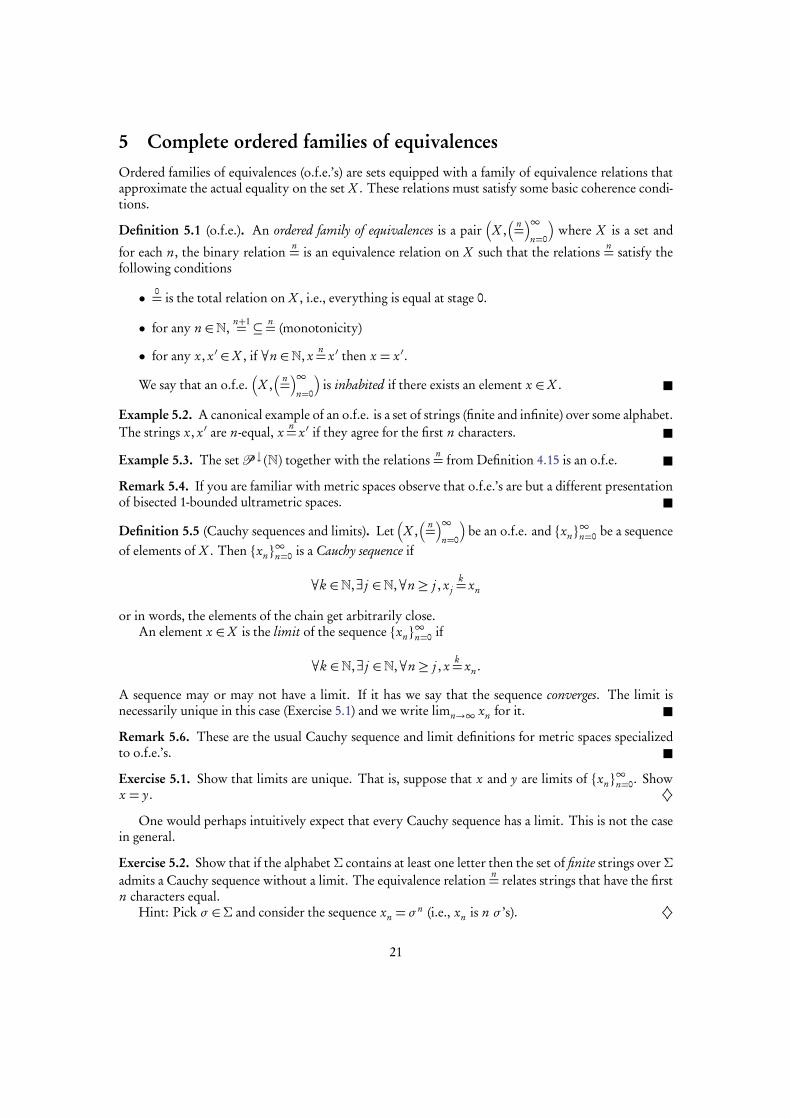
5 Complete ordered families of equivalencesOrdered families of equivalences (o.f.e.’s) are sets equipped with a family of equivalence relations thatapproximate the actual equality on the set X . These relations must satisfy some basic coherence condi-tions.

Definition 5.1 (o.f.e.). An ordered family of equivalences is a pair

X , n=∞

n=0

where X is a set and

for each n, the binary relation n= is an equivalence relation on X such that the relations n= satisfy thefollowing conditions

• 0= is the total relation on X , i.e., everything is equal at stage 0.

• for any n ∈N, n+1= ⊆ n= (monotonicity)

• for any x, x ′ ∈X , if ∀n ∈N, x n= x ′ then x = x ′.

We say that an o.f.e.

X , n=∞

n=0

is inhabited if there exists an element x ∈X .

Example 5.2. A canonical example of an o.f.e. is a set of strings (finite and infinite) over some alphabet.The strings x, x ′ are n-equal, x n= x ′ if they agree for the first n characters.

Example 5.3. The setP ↓ (N) together with the relations n= from Definition 4.15 is an o.f.e.

Remark 5.4. If you are familiar with metric spaces observe that o.f.e.’s are but a different presentationof bisected 1-bounded ultrametric spaces.

Definition 5.5 (Cauchy sequences and limits). Let

X , n=∞

n=0

be an o.f.e. and xn∞n=0 be a sequence

of elements of X . Then xn∞n=0 is a Cauchy sequence if

∀k ∈N,∃ j ∈N,∀n ≥ j , x jk= xn

or in words, the elements of the chain get arbitrarily close.An element x ∈X is the limit of the sequence xn

∞n=0 if

∀k ∈N,∃ j ∈N,∀n ≥ j , x k= xn .

A sequence may or may not have a limit. If it has we say that the sequence converges. The limit isnecessarily unique in this case (Exercise 5.1) and we write limn→∞ xn for it.

Remark 5.6. These are the usual Cauchy sequence and limit definitions for metric spaces specializedto o.f.e.’s.

Exercise 5.1. Show that limits are unique. That is, suppose that x and y are limits of xn∞n=0. Show

x = y. ♦

One would perhaps intuitively expect that every Cauchy sequence has a limit. This is not the casein general.

Exercise 5.2. Show that if the alphabet Σ contains at least one letter then the set of finite strings over Σadmits a Cauchy sequence without a limit. The equivalence relation n= relates strings that have the firstn characters equal.

Hint: Pick σ ∈Σ and consider the sequence xn = σn (i.e., xn is n σ ’s). ♦

21

We are interested in spaces which do have the property that every Cauchy sequence has a limit.These are called complete. Completeness allows us to have fixed points of suitable contractive functionswhich we define below.

Definition 5.7 (c.o.f.e.). A complete ordered family of equivalences is an ordered family of equivalences

X , n=∞

n=0

such that every Cauchy sequence in X has a limit in X .

Example 5.8. A canonical example of a c.o.f.e. is the set of infinite strings over an alphabet. Therelation n= relates streams that agree on at least the first n elements.

Exercise 5.3. Show the claims made in Example 5.8.Show that P ↓ (N) with relations from Definition 4.15 is a c.o.f.e. (We show a more general result

later in Proposition 5.12.) ♦

To have a category we also need morphisms between (complete) ordered families of equivalences.

Definition 5.9. Let

X , n=X

∞

n=0

and

Y, n=Y

∞

n=0

be two ordered families of equivalences and f afunction from the set X to the set Y . The function f is

• non-expansive if for any x, x ′ ∈X , and any n ∈N,

x n=X

x ′⇒ f (x) n=Y

f (x ′)

• contractive if for any x, x ′ ∈X , and any n ∈N,

x n=X

x ′⇒ f (x) n+1=Y

f (x ′)

Exercise 5.4. Show that non-expansive functions preserve limits, i.e., show that if f is a non-expansivefunction and xn

∞n=0 is a converging sequence, then so is f (xn)

∞n=0 and that

f

limn→∞

xn

= limn→∞

f (xn).

♦

The reason for introducing complete ordered families of equivalences, as opposed to just o.f.e.’s, isthat any contractive function on an inhabited c.o.f.e. has a unique fixed point.

Theorem 5.10 (Banach’s fixed point theorem). Let

X , n=∞

n=0

be a an inhabited c.o.f.e. and f : X →Xa contractive function. Then f has a unique fixed point.

Proof. First we show uniqueness. Suppose x and y are fixed points of f , i.e. f (x) = x and f (y) = y. Bydefinition of c.o.f.e.’s we have x 0= y. From contractiveness we then get f (x) 1= f (y) and so x 1= y. Thusby induction we have ∀n, x n= y. Hence by another property in the definition of c.o.f.e.’s we have x = y.

To show existence, we take any x0 ∈ X (note that this exists since by assumption X is inhabited).We then define xn+1 = f (xn) and claim that xn

n= xn+m for any n and m which we prove by inductionon n. For n = 0 this is trivial. For the inductive step we have, by contractiveness of f

xn+1 = f (xn)n+1= f (xn+m) = xn+m+1,

22

as required. This means that the sequence xn∞n=0 is Cauchy. Now we use completeness to conclude

that xn∞n=0 has a limit, which we claim is the fixed point of f . Let x = limn→∞ xn . We have (using

Exercise 5.4)

f (x) = f

limn→∞

xn

= limn→∞

f (xn) = limn→∞

xn+1 = limn→∞

xn = x

concluding the proof.

Definition 5.11 (The categoryU ). The categoryU of complete ordered families of equivalences hasas objects complete ordered families of equivalences and as morphisms non-expansive functions.

From now on, we often use the underlying set X to denote a (complete) o.f.e.

X , n=X

∞

n=0

, leavingthe family of equivalence relations implicit.

Exercise 5.5. Show thatU is indeed a category. Concretely, show that composition of non-expansivemorphisms is non-expansive and that the identity function is non-expansive. ♦

Exercise 5.6. Show that if f is contractive and g is non-expansive, then f g and g f are contractive.♦

Exercise 5.7. Show that the Set is a coreflective subcategory ofU . Concretely, this means that thereis an inclusion functor∆ : Set→U which maps a set X to a c.o.f.e. with equivalence relation n= beingthe equality on X for n > 0 and the total relation for 0.

Show that the functor ∆ is full and faithful and that it has a right adjoint, the forgetful functorF :U → Set that “forgets” the equivalence relations.

Further, show that the only contractive functions from any c.o.f.e. to∆(Y ) are constant. ♦

The last part of the exercise is one of the reasons why we can define fixed points of guarded recursivepredicates in theU hyperdoctrine which we describe below but not in a Set-based hyperdoctrine fromSection 4.5.

If we wish to find a fixed point of a function f from a set X to a set Y we really have nothing to goon. What the o.f.e.’s give us is the ability to get closer and closer to a fixed point, if f is well-behaved.What the c.o.f.e.’s additionally give us is that the “thing” we get closer and closer to is in fact an elementof the o.f.e.

5.1 U -based hyperdoctrineWe now wish to imitate the Set-based hyperdoctrine arising from a preordered set P ; the hyperdoctrinewith P = HomSet

−,P ↑ (P )

but in a way that would allow us also to model . in the logic. We canexpress this in a nice way by combiningP ↓ (N) withP ↑ (P ) into uniform predicates UPred (P ).

Let P be a preordered set. We define UPred (P )⊆P (N× P ) as

UPred (P ) = A∈P (N× P ) | ∀n ∈N, p ∈ P, (n, p) ∈A⇒∀m ≤ n,∀q ≥ p, (m, q) ∈A

i.e., they are sets downwards closed in the natural numbers and upwards closed in the order on P .Observe that UPred (P ) is nothing else thanP ↑ (Nop× P )where the order on the product is component-

wise and Nop are the naturals with the reverse of the usual order relation, i.e., 1 ≥ 2 ≥ 3 ≥ · · · . Thisimmediately gives us that UPred (P ) is a complete Heyting algebra (Exercise 4.6).

Proposition 5.12. For any preorder P , UPred (P ) is a c.o.f.e. with relation n= defined as

A n=B ⇐⇒ bAcn = bBcn

23

where

bAcn = (m,a) | (m,a) ∈A∧m < n

Proof. First we need to show that the specified data satisfies the requirements of an o.f.e. It is obviousthat all the relations are equivalence relations and that 0= is the total relation on UPred (P ). Regardingmonotonicity, suppose An+1= B . We need to show bAcn = bBcn and we do this by showing that they areincluded in one another. Since the two inclusions are completely symmetric we only show one.

Let (k ,a) ∈ bAcn . By definition (k ,a) ∈A and k < n which clearly implies that (k ,a) ∈ bAcn+1. The

assumption An+1= B gives us (k ,a) ∈ bBcn+1 but since k < n we also have (k ,a) ∈ bBcn concluding theproof of inclusion.

To show that the intersection of all relations n= is the identity relation suppose A n=B for all n. Weagain show that A and B are equal by showing two inclusions which are completely symmetric so itsuffices to show only one.

Suppose (m,a) ∈ A. By definition (m,a) ∈ bAcm+1, so from the assumption (m,a) ∈ bBcm+1 andthus (m,a) ∈ B , showing that A⊆ B .

We are left with showing completeness. Suppose An∞n=0 is a Cauchy sequence. Recall that this

means that for each n ∈ N there exists an Nn , such that for any j ≥ Nn , ANn

n=Aj . Because of the

monotonicity of the relations n= we can assume without loss of generality that N1 ≤N2 ≤N3 ≤ · · · .Define A=

¦

(m,a) | (m,a) ∈ANm+1

©

. We claim that A is the limit of An∞n=0.

First we show that A is in fact an element of UPred (P ). Take (m,a) ∈A and n ≤ m and b ≥ a. Weneed to show (n, b ) ∈A. By definition this means showing (n, b ) ∈ANn+1

. Recall that Nn+1 ≤Nm+1 byassumption and from the definition of the numbers Nk we have

ANn+1

n+1= ANm+1

which again by definition means

ANn+1

n+1=

ANm+1

n+1. But note that by the fact that ANm+1

is an

element of UPred (P ) we have (n, b ) ∈ANm+1and from this we have

(n, b ) ∈

ANm+1

n+1=

ANn+1

n+1⊆ANn+1

showing that (n, b ) ∈ANn+1.

Exercise 5.8. Using similar reasoning show that A n=ANn. ♦

The only thing left to show is that A is in fact the limit of UPred (P ). Let n ∈ N and k ≥ Nn . Wehave

Akn=ANn

n=A.

Thus for each n ∈ N there exists a Nn such that for every k ≥ Nn , Akn=A, i.e., A is the limit of the

sequence An∞n=0.

Exercise 5.9. UPred (P ) can be equivalently presented as monotone functions fromNop toP ↑ (P )withthe relation n= being

ϕn=ψ ⇐⇒ ∀k < n,ϕ(k) =ψ(k).

24

Show that there exist two non-expansive functions

Φ : UPred (P )→

Nop mon→ P ↑ (P )

Ψ :

Nop mon→ P ↑ (P )

→UPred (P )

that are mutually inverse, i.e., UPred (P ) and Nop mon→ P ↑ (P ) are isomorphic objects in the categoryU . Conclude that this means that Nop→P ↑ (P ) is also a complete ordered family of equivalences. ♦

Exercise 5.10. UPred (P ) can also be equivalently presented as monotone functions from P to thecomplete Heyting algebraP ↓ (N) with the relations being

ϕn=ψ ⇐⇒ ∀p ∈ P,ϕ(p) n=ψ(p)

Concretely, show that the functions

α :

Nop mon→ P ↑ (P )

→

Pmon→ P ↓ (N)

β :

Pmon→ P ↓ (N)

→

Nop mon→ P ↑ (P )

defined as

α(ϕ)(p) = n | p ∈ ϕ(n)β( f )(n) = p | n ∈ ϕ(p)

are well defined, non-expansive and mutually inverse. Conclude that this means that Pmon→ P ↓ (N) is

also a complete ordered family of equivalences. ♦

This last presentation of UPred (P ) presents it as the subset of the exponential P ↓ (N)P consistingof monotone functions. To make P an object ofU we equip it with a sequence of identity relations.

Exercise 5.11. Show that UPred (P ) is not isomorphic (inU ) to∆(X ) for any set X (see Exercise 5.7).♦

Proposition 5.13. The category U is cartesian closed. The terminal object is the singleton set (with theunique family of relations). If X and Y are objects ofU then the product object X ×Y is

X ×Y,

n=X×Y

∞

n=0

where

(x, y) n=X×Y(x ′, y ′) ⇐⇒ x n=

Xx ′ ∧ y n=

Yy ′

and the exponential object Y X is

HomU (X ,Y ) ,

n=Y X

∞

n=0

where

f n=Y X

g ⇐⇒ ∀x ∈X , f (x) n=Y

g (x).

is the exponential object.

25

Note that the underlying set of the exponential Y X consists of the non-expansive functions fromthe underlying set of X to the underlying set of Y .

Exercise 5.12. Prove Proposition 5.13. ♦

Proposition 5.14. Let Y be an object of U and P a preordered set. Then HomU (Y,UPred (P )) is acomplete Heyting algebra for operations defined pointwise.

Proof. Since UPred (P ) is a complete Heyting algebra we know from Exercise 4.3 that the set of allfunctions from the set X to UPred (P ) is a complete Heyting algebra for operations defined pointwise.Thus we know that the operations satisfy all the axioms of a complete Heyting algebra, if they are well-defined. That is, if all operations preserve non-expansiveness of functions. This is what we need tocheck.

We only show it for⇒. The other cases follow exactly the same pattern.Recall that the definition of⇒ in UPred (P ) is

A⇒ B = (n, p) | ∀k ≤ n,∀q ≥ p, (k , q) ∈A⇒ (k , q) ∈ B .

We first show that if A n=A′ and B n=B ′ then A⇒ B n=A′ ⇒ B ′ by showing two inclusions. The twodirections are symmetric so we only consider one.

Let (m, p) ∈ bA⇒ Bcn . By definition m < n and (m, p) ∈ A⇒ B and we need to show (m, p) ∈bA′⇒ B ′cn . Since we know that m < n it suffices to show (m, p) ∈A′⇒ B ′ and for this take k ≤ m andq ≥ p and assume (k , q) ∈ A′. Observe that k < n and since A n=A′ we have (k , q) ∈ A which implies(k , q) ∈ B which implies, using the fact that B n=B ′ and k < n that (k , q) ∈ B ′.

Suppose now that f , g : X →UPred (P ) are non-expansive and x, x ′ ∈X such that x n= x ′. Then bydefinition of operations we have

( f ⇒ g )(x) = ( f (x)⇒ g (x)) n=

f (x ′)⇒ g (x ′)

= ( f ⇒ g )(x ′)

where we used the fact that⇒ is “non-expansive” in UPred (P ) (shown above) and non-expansivenessof f and g to get n= in the middle.

Recall the motivation for going to the categoryU ; we wanted to be able to talk about guarded recur-sive functions in general. Similarly to the Heyting algebraP ↓ (N) there is an operation . on UPred (P )defined as

.(A) = (0, p) | p ∈ P ∪ (n+ 1, p) | (n, p) ∈A .

Exercise 5.13. Show that . is contractive. ♦

This . can be extended pointwise to the complete Heyting algebra HomU (Y,UPred (P )) for anyc.o.f.e. Y and is also contractive (when HomU (Y,UPred (P )) is equipped with the metric defined inProposition 5.13).

Proposition 5.15. Let M be a partial commutative monoid. The complete Heyting algebra UPred (M )arising from the extension order on M is a complete BI-algebra for the following operations

I =N×MA?B = (n,a · b ) | (n,a) ∈A, (n, b ) ∈ B ,a#b

A→?B = (n,a) | ∀m ≤ n,∀b#a, (m, b ) ∈A⇒ (m,a · b ) ∈ B

26

Exercise 5.14. Prove Proposition 5.15. ♦

With Propositions 5.13, 5.14 and 5.15 we have shown the following.

Theorem 5.16. Let M be a partial commutative monoid. The categoryU together with the generic objectUPred (M ) is a BI-hyperdoctrine.

We can generalize this construction further, replacing UPred (M ) by any other c.o.f.e. whose un-derlying set is a complete BI-algebra with a ..

Definition 5.17. A Löb BI-algebra is a c.o.f.e.

H , n=∞

n=0

whose underlying set H is a complete BI-algebra H with a monotone and contractive operation . : H → H satisfying h ≤ .(h) (monotonicity)and whenever .(h)≤ h then h => (Löb rule).

Further, the BI-algebra operations have to be non-expansive. For instance if I is any index set andfor each i ∈ I , ai

n= bi , then we require∧

i∈I

ain=∧

i∈I

bi

∨

i∈I

ain=∨

i∈I

bi

to hold.Additionally, . is required to satisfy the following equalities

.>=>

.

∧

i∈I

Ai

=∧

i∈I

.Ai

.

∨

i∈I

Ai

=∨

i∈I

.Ai if I 6= ;

.(A⇒ B) = .A⇒ .B.(A?B) = .(A) ? .(B).(A→?B) = .(A)→? . (B)

Remark 5.18. In the definition of a Löb BI-algebra we included the requirements that are satisfied by allthe examples we consider below. However, it is not clear whether all of the requirements are necessaryfor applications of the logic or whether they could be weakened (for instance, whether we should require.(A?B) = .(A) ? .(B) or not).

Example 5.19. If M is a partial commutative monoid then UPred (M ) is a Löb BI-algebra.

We then have the following theorem. The proof is much the same as the proof of Proposition 5.14.The requirement that the BI-algebra operations are non-expansive implies that the operations definedpointwise will preserve non-expansiveness of functions.

Theorem 5.20. Let H be a Löb BI-algebra. Then HomU (−, H ) is a BI-hyperdoctrine for operations definedpointwise that also validates rules involving . from Section 4.5.1.

27

Recall again the motivation for introducing c.o.f.e.’s from Section 4.5 and Example 4.17. If we useda Set-based hyperdoctrines we could choose to interpret the signature in such a way that even thoughwe guarded free variables using a ., we would have no fixed points since the interpretations of functionsymbols were arbitrary functions.

However in aU -based hyperdoctrine we must interpret all function symbols as non-expansive func-tions since these are the only morphisms inU . We thus have the following theorem and corollary forthe hyperdoctrine HomU (−, H ) for a Löb BI-algebra H .

Theorem 5.21. Assume ϕ satisfies Γ , p : Propτ ,∆ ` ϕ : σ and suppose further that all free occurrences of pin ϕ occur under a .. Then for each γ ∈ JΓ K and δ ∈ J∆K,

JΓ , p : Propτ ,∆ ` ϕ : σK (γ ,−,δ) : JPropτK→ JσK

is contractive.

Proof. We proceed by induction on the typing derivation Γ , p : Propτ ,∆ ` ϕ : σ and show some selectedrules.

• Suppose the last rule used was

Γ , p : Propτ ,∆ ` ϕ : Prop

Γ , p : Propτ ,∆ ` .ϕ : Prop.

Then by definition, the interpretation JΓ , p : Propτ ,∆ ` ϕ : PropK (γ ,−,δ) is non-expansive foreach γ and δ (this is because it is interpreted as a morphism inU ). By definition, the interpreta-tion

JΓ , p : Propτ ,∆ ` .ϕ : PropK= . JΓ , p : Propτ ,∆ ` ϕ : PropK

and so

JΓ , p : Propτ ,∆ ` .ϕ : PropK (γ ,−,δ) = . JΓ , p : Propτ ,∆ ` ϕ : PropK (γ ,−,δ).

Exercises 5.13 and 5.6 then give us that JΓ , p : Propτ ,∆ ` .ϕ : PropK (γ ,−,δ) is contractive. Notethat we have not used the induction hypothesis here and in fact we could not since p might notbe guarded anymore when we go under a ..

• Suppose that the last rule used was the function symbol rule. For simplicity assume that F hasonly two arguments so that the last rule used was

Γ , p : Propτ ,∆ `M1 : τ1 Γ , p : Propτ ,∆ `M2 : τ2

Γ , p : Propτ ,∆ ` F (M1, M2) : σ

To reduce clutter we write JM1K and JM2K for the interpretations of the typing judgments of M1and M2. By definition we have

JΓ , p : Propτ ,∆ ` F (M1, M2) : σK= JF K ⟨JM1K ,JM2K⟩ .

Since JF K is a morphism inU it is non-expansive. The induction hypothesis gives us that JM1K (γ ,−,δ)and JM2K (γ ,−,δ) are contractive. It is easy to see that then ⟨JM1K ,JM2K⟩ (γ ,−,δ) is also contrac-tive which gives us that JΓ , p : Propτ ,∆ ` F (M1, M2) : σK (δ,−,γ ) is also contractive (Exercise 5.6).

28

• Suppose the last rule used was the conjunction rule

Γ , p : Propτ ,∆ ` ϕ : Prop Γ , p : Propτ ,∆ `ψ : Prop

Γ , p : Propτ ,∆ ` ϕ ∧ψ : Prop

By definition,

JΓ , p : Propτ ,∆ ` ϕ ∧ψ : PropK= JϕK∧ JψK

and recall that the definitions of Heyting algebra operations on HomU (X , H ) are pointwise.Therefore JϕK ∧ JψK = ∧H ⟨JϕK ,JψK⟩ where on the right-hand side ∧H is the conjunction ofthe BI-algebra H . Using the induction hypothesis we have that JϕK (γ ,−,δ) and JψK (γ ,−,δ) arecontractive. By assumption that H is a Löb BI-algebra we have that ∧H is non-expansive givingus, using Exercise 5.6 that JΓ , p : Propτ ,∆ ` ϕ ∧ψ : PropK (γ ,−,δ) is contractive.

The other cases are similar.

Corollary 5.22. Assume ϕ satisfies Γ , p : Propτ ` ϕ : Propτ and suppose further that all free occurrences ofp in ϕ occur under a .. Then for each γ ∈ JΓ K there exists a unique hγ ∈ JPropτK such that

JΓ , p : Propτ ` ϕ : PropτK

γ , hγ

= hγ

and further, this assignment is non-expansive, i.e., if γ n=γ ′ then hγn= hγ ′ .

Proof. Existence and uniqueness of fixed points follows from Theorem 5.10 and the fact that UPred (M )JτK

is always inhabited, since UPred (M ) is.Non-expansiveness follows from non-expansivness of JΓ , p : Propτ ` ϕ : PropτK and the fact that if

two sequences are pointwise n-equal, so are their respective limits (see the construction of fixed pointsin Theorem 5.10).

Using these results we can safely add fixed points of guarded recursively defined predicates as inSection 4.5 to the logic and moreover, we can add rules stating uniqueness of such fixed points (up toequivalence ⇐⇒ ).

6 Constructions on the category UThe . is useful when we wish to construct fixed points of predicates, i.e., functions with codomainsome Löb BI-algebra. For models of pure separation logic and guarded recursion we can use uniformpredicates as shown above. Pure separation logic provides us with a way to reason about programs thatmanipulate dynamically allocated mutable state by allowing us to assert full ownership over resources.In general, however, we also wish to specify and reason about shared ownership over resources. This isuseful for modeling type systems for references, where the type of a reference cell is an invariant that isshared among all parts of the program, or for modeling program logics that combine ideas from sepa-ration logic with rely-guarantee style reasoning, see, e.g., [BRS+11] and the references therein. In thesecases, the basic idea is that propositions are indexed over “worlds”, which, loosely speaking, contain adescription of those invariants that have been established until now. In general, an invariant can be anykind of property, so invariants are propositions. A world can be understood as a finite map from naturalnumbers to invariants. We then have that propositions are indexed over worlds which contain propo-sitions and hence the space of propositions must satisfy a recursive equation of roughly the followingform:

Prop= (N fin* Prop)→UPred (M ) .

29

For cardinality reasons, this kind of recursive domain equation does not have a solution in Set. In thissection we show that a solution to this kind of recursive domain equation can be found in the categoryU and, moreover, that the resulting recursively defined space will in fact give rise to a BI-hyperdoctrinethat also models guarded recursively defined predicates.

To express the equation precisely inU we will make use of the É functor:

Definition 6.1. The functor É is a functor onU defined as

É

X , n=∞

n=0

=

X , n≡∞

n=0

É ( f ) = f

where0≡ is the total relation and x

n+1≡ x ′ iff x n= x ′

Exercise 6.1. Show that the functor É is well-defined. ♦

Definition 6.2. The categoryU op has as objects complete ordered families of equivalences and a mor-phism from X to Y is a morphism from Y to X inU .

Definition 6.3. A functor F :U op ×U →U is locally non-expansive if for all objects X , X ′, Y , andY ′ inU and f , f ′ ∈HomU (X ,X ′) and g , g ′ ∈HomU (Y

′,Y ) we have

f n= f ′ ∧ g n= g ′⇒ F ( f , g ) n= F ( f ′, g ′).

It is locally contractive if the stronger implication

f n= f ′ ∧ g n= g ′⇒ F ( f , g ) n+1= F ( f ′, g ′).

holds. Note that the equalities are equalities on function spaces.

Proposition 6.4. If F is a locally non-expansive functor thenÉ F and F (Éop ×É) are locally contractive.Here, the functor F (Éop ×É) works as

(F (Éop ×É))(X ,Y ) = F (Éop (X ),É (Y ))

on objects and analogously on morphisms andÉop:U op→U op is justÉworking onU op (i.e., its definitionis the same).

Exercise 6.2. Show Proposition 6.4. ♦

6.1 A typical recursive domain equationWe now consider the typical recursive domain equation mentioned above.

Let X be a c.o.f.e. We write N fin* X for the set of finite partial maps from N to X (no requirement

of non-expansiveness).

Proposition 6.5. If X is a c.o.f.e. then the space Nfin* X is a c.o.f.e. when equipped with the following

equivalence relations

f n= g ⇐⇒ n = 0∨

dom ( f ) = dom (g )∧∀x ∈ dom ( f ) , f (x) n= g (x)

.

Exercise 6.3. Prove Proposition 6.5. The only non-trivial thing to check is completeness. For this, firstshow that for any Cauchy sequence fn

∞n=0 there is an n, such that for any k ≥ n, dom ( fk ) = dom ( fn).

Then the proof is similar to the proof that the set of non-expansive functions between c.o.f.e.’s is againcomplete. ♦

30

We order the space N fin*X by extension ordering, i.e.,

f ≤ g ⇐⇒ dom ( f )⊆ dom (g )∧∀n ∈ dom ( f ) , f (n) = g (n).

Note that this is the same order that we used for ordering the monoid of heaps in Example 4.9.

Theorem 6.6. Let H be a Löb BI-algebra and X a c.o.f.e. Suppose that the limits in H respect the orderon H , i.e., given two converging sequences an

∞n=0 and bn

∞n=0 such that for all n, an ≤ bn we also have

limn→∞ an ≤ limn→∞ bn .

Then the set of monotone and non-expansive functions fromNfin* to H with the metric inherited from

the space HomU

Nfin*X , H

is again a Löb BI-algebra.

Proof. We know that the set of non-expansive functions with operations defined pointwise is again a LöbBI-algebra, but that does not immediately imply that the set of monotone and non-expansive functionsis as well.

It is easy to see that limits of Cauchy sequences exists using the fact that limits in H preserve order.Exercise!

It is a standard fact that monotone functions from a preordered set into a complete Heyting algebraagain form a complete Heyting algebra for pointwise order and the operations defined as follows

( f ⇒ g )(x) =∧

y≥x

( f (y)⇒ g (y))

∧

i∈I

fi

(x) =∧

i∈I

( fi (x))

∨

i∈I

fi

(x) =∨

i∈I

( fi (x)) .

We first need to check that the operations are well defined. It is easy to see that given monotone functionsas input the operations produces monotone functions as output. It is also easy to see that

∧

and∨

preserve non-expansiveness. However proving non-expansiveness of f ⇒ g is not so straightforward.Suppose x n= x ′. The case when n = 0 is not interesting so assume n > 0. We need to show that

∧

y≥x

( f (y)⇒ g (y)) n=∧

y ′≥x ′( f (y ′)⇒ g (y ′)).

By the definition of the equality relation on N fin* X we have that dom (x)dom (x ′) and that for each

k ∈ dom (x) , x(k) n= x ′(k). By the definition of the order relation on N fin*X we have that if y ≥ x then

dom (y)⊇ dom (x) and for each k ∈ dom (x), x(k) = y(k) and similarly for x ′. Thus if y ≥ x and y ′ ≥ x ′

then ∀k ∈ dom (x) = dom (x ′) , y(k) n= y ′(k). Thus for each y ≥ x there exists a y ′ ≥ x ′, such that y n= y ′

and conversely, for each y ′ ≥ x ′ there exists a y ≥ x, such that y n= y ′.

Exercise 6.4. Let I and J be two index sets and n ∈N. Suppose that for each i ∈ I there exists a j ∈ J ,such that ai

n= b j and conversely that for each j ∈ J there exists an i ∈ I , such that ain= b j . Show that in

this case∧

i∈I

ain=∧

j∈J

b j .

Hint: Consider the extended index set K = I t J , the disjoint union of I and J . Define elements a′k andb ′k such that for each k ∈K , a′k

n= b ′k and so that∧

k∈K

a′k =∧

i∈I

ai

∧

k∈K

b ′k =∧

j∈J

b j .

Then use that∧

is non-expansive. ♦

31

Remark 6.7. Theorem 6.6 considers monotone functions on some particular c.o.f.e. Of course, thiscan be generalized to monotone functions on any suitable preordered c.o.f.e., see [BST10].

Now we know that the operations are well-defined. Next we need to show that they satisfy theHeyting algebra axioms.

Exercise 6.5. Show that operations so defined satisfy the Heyting algebra axioms. ♦

We also need to establish that the operations are non-expansive. Recall that equality on the functionspace is defined pointwise. We only consider the implication, the other operations are similar.

Suppose f n= f ′ and g n= g ′. We then have that for each y, ( f (y)⇒ g (y)) n=( f ′(y)⇒ g ′(y)) and fromthis it is easy to see that ( f ⇒ g ) n=( f ′⇒ g ′) by non-expansiveness of

∧

.It is easy to see that we can extend the operation . pointwise, i.e.,

.( f ) = . f .

Exercise 6.6. Show that the . defined this way satisfies all the requirements. ♦

The BI-algebra operations are defined as follows

( f ? g )(x) = f (x) ? g (x) ( f →?g )(x) =∧

y≥x

( f (y)→?g (y)).

We can show in the same way as for ∧ and⇒ that they are well-defined and satisfy the correct axioms.

Given any partial commutative monoid we have, using Theorem 6.6, that the functor

F :U op→U

F (X ) = (N fin*X ) mon→

n.e .UPred (M )

is well-defined.The space of propositions will be derived from this functor. However in general this functor does

not have a fixed-point; we need to make it locally-contractive by composing with the functor É. UsingTheorem 6.9 (described in the next subsection) we have that G =É F has a unique fixed point whichwe call PreProp. That is, G(PreProp)∼= PreProp inU . Concretely, we have a non-expansive bijectionι with a non-expansive inverse

ι : G(PreProp)→ PreProp.

Since PreProp is a c.o.f.e. we can use Theorem 6.6 to show that the space

Prop= F (PreProp) = (N fin* PreProp) mon→

n.e .UPred (M )

is a Löb BI-algebra. Hence the hyperdoctrine HomU (−,Prop) is a BI-hyperdoctrine that also modelsthe . operation and fixed points of guarded recursive predicates (Theorem 5.20).

32

Summary As a summary, we present the explicit model of propositions in the hyperdoctrine HomU (−,Prop)(we include equality, although we have not considered that earlier). Recall that a proposition in contextΓ ` ϕ : Prop is interpreted as a non-expansive function from JΓ K to Prop. Omitting : Prop from thesyntax, we have:

JΓ `M =τ NKγ w =¦

(n, r ) | JΓ `M : τKγn+1= JΓ `N : τKγ

©

JΓ `>Kγ w =N×M

JΓ ` ϕ ∧ψKγ w = JΓ ` ϕKγ w ∩ JΓ `ψKγ w

JΓ `⊥Kγ w = ;JΓ ` ϕ ∨ψKγ w = JΓ ` ϕKγ w ∪ JΓ `ψKγ w

JΓ ` ϕ⇒ψKγ w = ∀w ′ ≥ w,∀n′ ≤ n,∀r ′ ≥ r, (n′, r ′) ∈ JΓ ` ϕKγ w ′⇒ (n′, r ′) ∈ JΓ `ψKγ w ′

JΓ ` ∀x : σ ,ϕKγ w =⋂

d∈JσK

JΓ , x : σ ` ϕK(γ ,d )w

JΓ ` ∃x : σ ,ϕKγ w =⋃

d∈JσK

JΓ , x : σ ` ϕK(γ ,d )w

JΓ ` .ϕKγ w = (0, r ) | r ∈M ∪ (n+ 1, r ) | (n, r ) ∈ JΓ ` ϕKγ w

JΓ ` I Kγ w =N×M

JΓ ` ϕ ?ψKγ w = (n, r ) | ∃r1, r2, r = r1 · r2 ∧ (n, r1) ∈ JΓ ` ϕKγ w ∧ (n, r2) ∈ JΓ `ψKγ w

JΓ ` ϕ→?ψKγ w = (n, r ) | ∀w ′ ≥ w,∀n′ ≤ n,∀r ′#r.(n′, r ′) ∈ JΓ ` ϕKγ w ′ ∧ (n′, r · r ′) ∈ JΓ `ψKγ w ′

In particular note that the “resources” r are not used in the interpretation of equality.Moreover, when p occurs under a . in ϕ, then we have a recursively defined predicate:

JΓ `µp.ϕ : PropτKγ = fix(λx : JPropτK .JΓ , p : Propτ ` ϕ : PropτK(γ ,x))

Here fix yields the fixed point of the contractive function, see Corollary 5.22.Finally, we can have a new logical connective for expressing invariants. Syntactically

Γ `M :N Γ ` ϕ : Prop

Γ ` ϕ M : Prop

whereN is a base type, which we interpret by the natural numbers (formally, as the object∆(N) inU ).Then we define

rΓ ` ϕ M

z

γw =

¦

(n, r ) | w(JΓ `M Kγ )n+1= ι(JΓ ` ϕKγ )

©

.

Let us unfold the definition to see what it means and to see that it makes sense. First, given γ ∈ JΓ Kwe have

JΓ `M Kγ ∈ JNK=∆(N)

JΓ ` ϕKγ ∈ JPropK= Prop= F (PreProp)

33

and we wish to haverΓ ` ϕ M : Prop

z

γ∈ JPropK= Prop= (N fin

* PreProp) mon→n.e .

UPred (M ) .

Thus given w ∈N fin* PreProp we wish to have

rΓ ` ϕ M : Prop

z

γw ∈UPred (M ) .

Now since the underlying set of∆(N) isNwe have w(JΓ `M Kγ ) ∈ PreProp. Recall the isomorphismι :É (F (PreProp))→ PreProp. Since the underlying set ofÉ (F (PreProp)) is the same as the underlyingset of F (PreProp) we can apply ι to JΓ ` ϕKγ to get

ι

JΓ ` ϕKγ

∈ PreProp

We then compare for n-equality in the space PreProp.Now what the definition is supposed to express is that if (n, r ) is in

rΓ ` ϕ M : Prop

z

γw for some

world w, then the invariant for region M in world w is approximately ϕ, where approximately is ex-pressed using n-equality and means, intuitively, that ϕ cannot be distinguished from the invariant forM in w for n steps. The use of the isomorphism ι is necessary only because we do not have a solutionof the domain equation up to equality, but only up to an isomorphism.

Observe also that therΓ ` ϕ M : Prop

z

γw is oblivious to resources (to r ∈M ).

Exercise 6.7. Check that the interpretation ofrΓ ` ϕ M : Prop

zis well defined. Concretely, check that

rΓ ` ϕ M : Prop

zis non-expansive and that for each γ ∈ Γ , the function

rΓ ` ϕ M : Prop

z

γ

is an element of F (PreProp) which means that it is non-expansive and monotone in the world w andactually maps into UPred (M ). ♦

6.2 Explicit construction of fixed points of locally contractive functors in UIn this subsection, we present an elementary construction of the fixed point of a locally contractivefunctor in the category of complete ordered families of equivalences. This fixed point theorem is origi-nally due to America and Rutten [AR89]. In [BST10] one can find a category-theoretic generalization,which shows how to obtain fixed points of locally contractive funtors on categories enriched inU . It isnot necessary to understand the proof in this subsection to understand the rest of the material in thesenotes.

Definition 6.8. A fixed point of a locally contractive functor F is an object X ∈U , such that F (X ,X )∼=X .

Theorem 6.9. Every locally contractive functor F such that F (1,1) is inhabited has a unique fixed point.The fixed point is unique among inhabited c.o.f.e.’s.

If in addition F (;,;) is inhabited then the fixed point of F is unique.

34

Proof. We first construct a solution. Then show uniqueness.Define a sequence of spaces Fn ∈U by induction as follows:

F0 = (∗, (=)∞n=0)

Fn+1 = F (Fn , Fn)

together with projections pn : Fn+1→ Fn and embeddings en : Fn→ Fn+1

p0 = the unique map to F0

pn+1 = F (en , pn)e0 = any map from F0 to F1

en+1 = F (pn , en)

Note that e0 exists because by assumption F (1,1) is inhabited and constant functions are non-expansive.Later we will need the fact that ek and pk are indeed embeddings and projections, i.e., that

∀k , pk ek = idFk. (6)

which we show by induction. The base case is trivial. For the inductive case we have

pk+1 ek+1 = F (ek , pk ) F (pk , ek ) = F (pk ek , pk ek ) = F

idFk, idFk

= idFk+1.

Projection followed by an embedding does not equal the identity function, but it does get closerwith increasing k. More precisely, we have

∀k , ek pkk= idFk+1

(7)

The base case is trivial, since everything is equal at step 0. For the inductive step we have

ek+1 pk+1 = F (pk , ek ) F (ek , pk ) = F (ek pk , ek pk )k+1= idFk+2

the last equation holding by the induction hypothesis and contractiveness of F . This is the place wherelocal contractiveness of F is used.

It will be convenient later to use compositions of embeddings e`k : Fk → F` and projections p`k : F`→Fk which we define as

pkk = idFk

pk+`+1k = pk+`

k pk+`

ekk = idFk

ek+`+1k = ek+` ek+`

k

Exercise 6.8. Show that for any `≥ k,

p`k e`k = idFk. (8)

♦

Hint: Use (6).We claim that

X =¨

x ∈∏

n∈NFn

∀k , pk

xk+1

= xk

«

35

is a fixed point of F , i.e., that F (X ,X )∼=X . The equality on X is defined as

x n=X x ′ ⇐⇒ ∀k , xkn=Fk

x ′k

where n=Fkdenotes n-th equivalence relation on the set Fk .

It is easy to see that

X , n=∞

n=0

is indeed an object ofU . In fact, it is also inhabited, for instance

en0 (∗)

∞n=0 is an element of X which is easy to see using (8).

To construct an isomorphism between X and F (X ,X )we will need auxiliary embeddings ιn : Fn→X and projections πn : X → Fn defined as follows

πn(x) = xn (ιn(y))k =¨

pnk (y) if n ≥ k

ekn (y) if k ≥ n

Using (8) it is easy to see that ιn is well defined for any n and since pk and ek are non-expansive, so arepn

k and ekn and consequently also ιn (see definition of equality on X ).

Using these we can define morphism α : X → F (X ,X ) and β : F (X ,X ) → X and show themmutually inverse. They are defined as follows

β(z)n =¨

∗ if n = 0F (ιm ,πm)(z) if n = m+ 1

and

α(x) = limk→∞

F (πk , ιk )

xk+1

We first need to make sure that these are good definitions, i.e., that they do indeed define morphismin U between X and F (X ,X ). First we consider β. To be well-defined it has to actually map into Xand be non-expansive. To see that it maps into X we proceed by induction. The base case is trivial sinceF1 is a single-element space. For the inductive case we have

pn+1

β(z)n+2

= pn+1

F (ιn+1,πn+1)(z)

= F (en , pn)

F (ιn+1,πn+1)(z)

= F

ιn+1 en , pn πn+1

(z) = F (ιn ,πn)(z) =β(z)n+1

where we have used the fact, which is easily checked, that ιn+1 en = ιn and pn πn+1 =πn .The fact that β is non-expansive follows directly from the fact that F (ιm ,πm) is non-expansive for

all m, since F is a functor mapping intoU .To see that α is well-defined we have to first show that the limit used in its definition actually exists.

Recall that we are working with c.o.f.e.’s so we only need to check that the sequence

F (πk , ιk )

xk+1

∞k=0

is a Cauchy chain for x ∈X .We will show that

F (πk , ιk )

xk+1

k+1= F

πk+`, ιk+`

xk+`+1

for any ` with the equality being the equality in F (X ,X ).We proceed by induction on ` with the base case being trivial by construction.

F (πk , ιk )

xk+1

= F (πk , ιk )

pk+1xk+2

= F (πk , ιk )

F (ek , pk ) (xk+2)

= F (ek πk , ιk pk )

xk+2

36

and from (7) we have

ek (πk (y)) = ek (pk (πk+1(y)))k=πk+1(y)

since πk = pk πk+1 and

ιk (pk (y)) = ιk+1(ek (pk (y)))k= ιk+1(y)

since ιk+1 ek = ιk . Combining these together with the fact that F is contractive we have

F (ek πk , ιk pk )

xk+2

k+1= F

πk+1, ιk+1

xk+2

and using the induction hypothesis for ` we get

F

πk+1, ιk+1

xk+2

k+1= F

πk+1+`, ιk+1+`

xk+2+`

= F

πk+`+1, ιk+`+1

xk+1+`+1

concluding the proof.We have thus established that the sequence used in the definition of α is a Cauchy chain, hence it

has a limit by completeness.

Exercise 6.9. It is a good exercise to show that α is non-expansive or more generally, that given twoCauchy-chain that are pointwise n-equal, then the limits are also n-equal. That is, given two Cauchy-

chains an∞n=0 and bn

∞n=0 such that ∀n,an

k= bn , then limn→∞ ank= limn→∞ bn . ♦

Thus we have α and β, two non-expansive maps. Now we need to show that they are inverses. Wefirst consider α β.

(α β)(z) = limk→∞

F (πk , ιk ) (F (ιk ,πk )(z)) = limk→∞

F (ιk πk , ιk πk )(z)

We wish to show that the limit is z. To that end we show that ιk πkk= idX . Let x ∈ X . We have for

`≥ k

ιk (πk (x))` =¨

x` if `≤ ke`k (xk ) if k ≤ `

so clearly ιk (πk (x))`k= x` for `≤ k. For k ≤ ` we have

ιk (πk (x))` = e`k (xk ) = e`k (p`k (x`))

k= x`

where we have used

Exercise 6.10. Show that for any `≥ k, e`k p`kk= idF`

. ♦

Hint: Use induction and (7).Since F is contractive we have shown that z is the limit of limk→∞ F (ιk πk , ιk πk )(z) and so

α(β(z)) = z.To show β(α(x)) = x we proceed as follows

β(α(x))n+1 = F (ιn ,πn)

limk→∞

F (πk , ιk )

xk+1

and since non-expansive functions preserve limits we get

limk→∞

F (ιn ,πn)

F (πk , ιk )

xk+1

= limk→∞

F (πk ιn ,πn ιk )

xk+1

37

Exercise 6.11. For k ≥ n we have πk ιn = ekn and πn ιk = pk

n and additionally F (ekn , pk

n ) = pk+1n+1 . ♦

Using the result of the last exercise we get

limk→∞

F (πk ιn ,πn ιk )

xk+1

= limk→∞

pkn+1(xk+1) = lim

k→∞xn+1 = xn+1

concluding the proof that β α= idX .Now to show uniqueness (up to isomorphism) suppose Y is another inhabited solution, i.e., γ :

F (Y,Y )∼= Y . We need to show there is an isomorphism between X and Y and we proceed similarly aswe did in the construction of an isomorphisms between F (X ,X ) and X .

Define embedding projection pairs ξn : Y → Fn and ζn : Fn→ Y by induction as

ξ0 = the unique map to F0

ξn+1 = F (ζn ,ξn) γ−1

ζ0 = the unique map such that γ F (ξ0,ζ0) e0 = ζ0

ζn+1 = γ F (ξn ,ζn)

Then define ε : Y →X as ε(y)n = ξn(y) and δ : X → Y as δ(x) = limk→∞ ζk (πk (x)).

Exercise 6.12. Show that ζ0 is well-defined, that is, that there is a unique map ζ0 : F0 → Y , such thatγ F (ξ0,ζ0)e0 = ζ0. Hint: define a contractive function on HomU (F0,Y ) using the required property.

♦

Exercise 6.13. Show that for all n we have pn ξn+1 = ξn and ζn+1 en = ζn . Further, show thatξn ζn = idFn

. Using these show that for n ≥ k we have ξn ζk = enk . ♦

Exercise 6.14. Show that ε and δ are well-defined, non-expansive and mutually inverse. Additionallyshow that γ F (ε,δ) = δ β. For the last part notice that ε = limn→∞ ιn ξn by using the fact thatlimn→∞ ιn πn = idX . Then use the fact that F , being locally contractive, preserves limits on hom-sets. ♦

Exercise 6.15. Find an example of a locally contractive functor that has two fixed points, an inhabitedone and ;. ♦

7 Further Reading — the Topos of TreesThe first hyperdoctrine we considered in these notes was the one for the set-theoretic model of higher-order logic, namely Set with 2 as the generic object. One of the particular properties of this hyperdoc-trine is that HomSet (X , 2) is naturally isomorphic to subobjects of X . In other words, 2 is a subobjectclassifier in Set. A topos is a cartesian closed category with a subobject classifier.

The categoryU is a full subcategory of the topos of treesS , which is the category of presheaves overthe natural numbers. The É functor extends to S and one can also find solutions to recursive domainequations in S . See [BMSS12] for a discussion of that and also for an application to a “synthetic”step-indexed model of a programming language with dynamically allocated references. In [SB14], S isused as the ambient logic in which a model of a program logic called iCAP is defined. We emphasize,however, that the model of iCAP can also be given more explicitly using the approach detailed in theprevious section.

38

References[AR89] P. America and J. J. M. M. Rutten. Solving reflexive domain equations in a category of

complete metric spaces. J. Comput. Syst. Sci., 39(3):343–375, 1989.

[Awo10] S. Awodey. Category Theory. Oxford Logic Guides. Oxford University Press, 2010.

[BBTS07] Bodil Biering, Lars Birkedal, and Noah Torp-Smith. Bi-hyperdoctrines, higher-order sepa-ration logic, and abstraction. ACM Trans. Program. Lang. Syst., 29(5), August 2007.

[BMSS12] L. Birkedal, R. Møgelberg, J. Schwinghammer, and K. Støvring. First steps in syntheticguarded domain theory: step-indexing in the topos of trees. Logical Methods in ComputerScience, 8(4), October 2012.

[BRS+11] L. Birkedal, B. Reus, J. Schwinghammer, K. Støvring, J. Thamsborg, and H. Yang. Step-indexed kripke models over recursive worlds. In Thomas Ball and Mooly Sagiv, editors,Proceedings of the 38th ACM SIGPLAN-SIGACT Symposium on Principles of ProgrammingLanguages, POPL 2011, Austin, TX, USA, January 26-28, 2011, pages 119–132. ACM, 2011.

[BST10] L. Birkedal, K. Støvring, and J. Thamsborg. The category-theoretic solution of recursivemetric-space equations. Theor. Comput. Sci., 411(47):4102–4122, 2010.

[Jac99] B. Jacobs. Categorical Logic and Type Theory, volume 141 of Studies in Logic and the Founda-tions of Mathematics. North-Holland Publishing Co., Amsterdam, 1999.

[Law69] F.W. Lawvere. Adjointness in foundations. Dialectica, 23(3/4):281–296, 1969.

[Pit02] A. M. Pitts. Tripos theory in retrospect. Math. Structures Comput. Sci., 12(3):265–279, 2002.

[SB14] K. Svendsen and L. Birkedal. Impredicative Concurrent Abstract Predicates. In Proceedingsof ESOP, 2014.

39

Rules for manipulation of contexts

Γ ` ϕ : Prop

Γ | ϕ ` ϕIDENTITY

Γ | Θ ` ϕ Γ | Ξ,ϕ `ψΓ | Θ,Ξ `ψ

CUTΓ | Θ ` ϕ Γ `ψ : Prop

Γ | Θ,ψ ` ϕWEAK-PROP

Γ | Θ,ϕ,ϕ `ψΓ | Θ,ϕ `ψ

CONTR-PROPΓ | Θ,ϕ,ψ,Ξ ` χΓ | Θ,ψ,ϕ,Ξ ` χ

EXCH-PROPΓ | Θ ` ϕ

Γ , x : σ | Θ ` ϕWEAK-TYPE

Γ , x : σ , y : σ | Θ ` ϕΓ , x : σ | Θ [x/y] ` ϕ [x/y]

CONTR-TYPEΓ , x : σ , y : ρ,∆ | Θ ` ϕΓ , y : ρ, x : σ ,∆ | Θ ` ϕ

EXCH-TYPE

Γ `M : σ ∆, x : σ ,∆′ | Θ `ψ∆,Γ ,∆′ | Θ [M/x] `ψ [M/x]

SUBSTITUTION

Rules for introduction and elimination of connectives

Γ | Θ `>TRUE

Γ | Θ,⊥`ψFALSE

Γ | Θ ` ϕ Γ | Θ `ψΓ | Θ ` ϕ ∧ψ

AND-IΓ | Θ ` ϕ ∧ψΓ | Θ ` ϕ

AND-E1Γ | Θ ` ϕ ∧ψΓ | Θ `ψ

AND-E2

Γ | Θ ` ϕΓ | Θ ` ϕ ∨ψ

OR-I1Γ | Θ `ψΓ | Θ ` ϕ ∨ψ

OR-I2Γ | Θ,ϕ ` χ Γ | Θ,ψ ` χ

Γ | Θ,ϕ ∨ψ ` χOR-E

Γ | Θ,ϕ `ψΓ | Θ ` ϕ⇒ψ

IMP-IΓ | Θ ` ϕ⇒ψ Γ | Θ ` ϕ

Γ | Θ `ψIMP-E

Γ , x : σ | Θ ` ϕΓ | Θ ` ∀x : σ ,ϕ

∀-IΓ `M : σ Γ | Θ ` ∀x : σ ,ϕ

Γ | Θ ` ϕ [M/x]∀-E

Γ `M : σ Γ | Θ ` ϕ [M/x]Γ | Θ ` ∃x : σ ,ϕ

∃-IΓ | Θ ` ∃x : σ ,ϕ Γ , x : σ | Ξ,ϕ `ψ

Γ | Θ,Ξ `ψ∃-E

Figure 3: Natural deduction rules for higher-order logic. Note that by convention x does not appearfree in Θ, Ξ or ψ in the rules ∀-I and ∃-E since we implicitly have that x is not in Γ and Θ, Ξ and ψ arewell formed in context Γ .

40

Interpretation of types assuming a chosen interpretation of base types. We write X ×Y and X Y for theproduct and exponential in C respectively.

J1K= 1Jσ ×τK= JσK× JτK

Jσ→ τK= JτKJσK

Interpretation of terms (including logical connectives) assuming interpretations of function symbols.We use δX = ⟨idX , idX , ⟩ : X → X ×X and ξX ,Y = ⟨π′,π⟩ : X ×Y → Y ×X . We use Λ ( f ) : X → ZY

for the transpose of a morphism f : X ×Y → Z and ε : X ×Y X → Y for the evaluation map.

Jx : σ ` x : σK= idJσK

JΓ , x : σ `M : τK= JΓ `M : τK πJΓ , x : σ `M [x/y] : τK= JΓ , x : σ , y : σ `M : τK idJΓK×δJσK

qΓ , x : σ ′, y : σ ,∆ `M [y/x, x/y] : τ

y=

qΓ , x : σ , y : σ ′,∆ `M : τ

y idJΓK× ξJσ ′K,JσK× idJ∆K

qΓ ` F (M1, . . . , Mn) : τn+1

y= JF K ⟨JΓ `Mi : τiK⟩

ni=1

JΓ ` ⟨M ,N ⟩ : τ×σK= ⟨JΓ `M : τK ,JΓ `N : σK⟩JΓ `π1 M : τK=π JΓ `M : τ×σK

JΓ `π2 M : τK=π′ JΓ `M : τ×σKJΓ ` λx.M : σ→ τK=Λ (JΓ , x : σ `M : τK)

JΓ `M N : σK= ε ⟨JΓ `N : τK ,JΓ `M : τ→ σK⟩JΓ `> : PropK=>JΓK

JΓ `⊥ : PropK=⊥JΓK

JΓ ` ϕ ∧ψ : PropK= JΓ ` ϕ : PropK∧JΓK JΓ `ψ : PropK

JΓ ` ϕ ∨ψ : PropK= JΓ ` ϕ : PropK∨JΓK JΓ `ψ : PropK

JΓ ` ϕ⇒ψ : PropK= JΓ ` ϕ : PropK⇒JΓK JΓ `ψ : PropK

JΓ ` ∀x : σ ,ϕ : PropK= ∀JσKJΓK (JΓ , x : σ ` ϕ : PropK)

JΓ ` ∃x : σ ,ϕ : PropK= ∃JσKJΓK (JΓ , x : σ ` ϕ : PropK)

Figure 4: Interpretation of higher-order logic in a hyperdoctrine.

41