1

A systematic path to non-Markovian dynamics:

New response pdf evolution equations under Gaussian coloured noise excitation

K.I. Mamis, G.A. Athanassoulis and Z.G. Kapelonis

konmamis@central.ntua.gr, mathan@central.ntua.gr, zkapel@central.ntua.gr

School of Naval Architecture & Marine Engineering, National Technical University of Athens

9 Iroon Polytechniou st., 15780 Zografos, GREECE

Abstract. Determining evolution equations governing the probability density function (pdf) of

non-Markovian responses to random differential equations (RDEs) excited by coloured noise, is

an important issue arising in various problems of stochastic dynamics, advanced statistical phys-

ics and uncertainty quantification of macroscopic systems. In the present work, such equations

are derived for a scalar, nonlinear RDE under additive coloured Gaussian noise excitation,

through the stochastic Liouville equation. The latter is an exact, yet non-closed equation, involv-

ing averages over the time history of the non-Markovian response. This nonlocality is treated by

applying an extension of the Novikov-Furutsu theorem and a novel approximation, employing a

stochastic Volterra-Taylor functional expansion around instantaneous response moments, leading

to efficient, closed, approximate equations for the response pdf. These equations retain a tractable

amount of nonlocality and nonlinearity, and they are valid in both the transient and long-time re-

gimes for any correlation function of the excitation. Also, they include as special cases various

existing relevant models, and generalize Hänggi’s ansatz in a rational way. Numerical results for

a bistable nonlinear RDE confirm the accuracy and the efficiency of the new equations. Exten-

sion to the multidimensional case (systems of RDEs) is feasible, yet laborious.

Keywords: uncertainty quantification, random differential equation, coloured noise excitation,

Novikov-Furutsu theorem, Volterra-Taylor expansion, Hänggi’s ansatz

TABLE OF CONTENTS

Abstract 1

1. Introduction 3

1(a) Nonlinear RDEs under coloured noise excitation and the corresponding stochastic

Liouville equation 4

1(b) New, closed probability evolution equations for non Markovian response 6

2. Transformed stochastic Liouville equation and some straightforward applications 6

2(a) Classical FPK equation for the nonlinear RDE under white noise excitation 8

2(b) Exact genFPK equation for the linear RDE under coloured noise excitation 9

2

2(c) Small correlation time genFPK equation 10

2(d) Fox’s genFPK equation 11

3. Novel genFPK equations under Volterra adjustable decoupling approximation 12

4. First numerical results 16

5. Conclusions and discussion 19

References (for the main paper) 20

Appendix A. Derivation of the stochastic Liouville equation via the delta projection method 24

A(a) Delta projection method 24

A(b) Derivation of the stochastic Liouville equation 26

A(c) Comparison of SLE derivation presented herein to van Kampen’s derivation 27

Appendix B. On the solvability of the genFPK equation corresponding to a linear RDE 30

B(a) Statement of the problem 30

B(b) Uniqueness of solution 31

B(c) Existence of solution and consistency with known results 33

Appendix C. Scheme of numerical solution. Implementation and validation 36

C(a) Partition of Unity and PU approximation spaces 36

C(b) Construction of cover, PU functions, and local basis functions for 1D domains 37

C(c) PUFEM discretization and numerical solution of pdf evolution equations 40

C(d) Validation of the proposed scheme for the linear case 43

C(e) Treatment of the nonlinear, nonlocal terms 44

Appendix D. Numerical Investigation of the range of validity of VADA genFPK equations 47

References (for the Appendices) 50

3

1. Introduction

The determination of the probabilistic structure of the response of a dynamical system to random

excitations is an important question for many problems in statistical physics, material sciences,

biomathematics, various engineering disciplines and elsewhere. In macroscopic stochastic dy-

namics it constitutes the basis of uncertainty quantification. For the special case of systems under

white noise excitation, the answer is well-formulated; the evolution of the transition probability

density function is governed by the Fokker-Planck-Kolmogorov (FPK) equation [1–3], [4] Sec.

5.6.6, [5] Ch. 5, [6] Sec. 6.3, [7] Sec. 3.18-9. In this case, the response is Markovian and, thus, its

complete probabilistic structure is defined by means of the transition pdf. Unfortunately, this

convenient description, via a single partial differential equation, is not applicable to problems

where the random excitations are smoothly correlated (coloured) noises, and thus the responses

are non-Markovian. The importance of coloured noise excitation in many advanced and real-life

applications, and the theoretical complicacies it induces(1), are discussed in many works, see e.g.

[8], [9], Sec. IX.7, [10–16]. Despite the difficulties, various methods seeking to formulate re-

sponse pdf evolution equations for systems under coloured noise excitation have been proposed

and developed.

The most straightforward approach, popular in engineering applications, is the filtering approach

[4] Sec. 5.10, [17,18]. In this case, the original system of random(2) differential equations (RDEs)

is augmented by a filter excited by white noise, whose output is utilized as an approximation of

the given coloured excitation. Thus, the augmented system admits an exact FPK description. This

approach is also called Markovianization by extension [19], or embedding in a Markovian pro-

cess of higher dimensions [8], Sec. VI.A. Filtering is also the starting point of unified coloured

noise approximation (UCNA) developed by Hänggi & Jung [20], [8] Sec. V.C. However im-

portant this approach may be, it has an inherent drawback; it leads to an inflation of the degrees

of freedom in the FPK equation, especially when an accurate approximation of the excitation cor-

relation is needed, in which case higher order filters are required.

An alternative approach is to try to derive pdf evolution equations analogous to the FPK equa-

tion, keeping only the natural degrees of freedom of the system, while taking into account the

given coloured noise excitation. The main difficulty here, coming from the fact that “non-

Markovian processes […] cannot be considered merely as corrections to the class of Markov pro-

cesses” [21], lies in the emergence of terms dependent on the whole time history of the response,

even for the one-time pdf evolution equation, as explained in detail subsequently. Therefore, clo-

sure techniques for the non-local term are needed, in order to obtain approximate, yet closed and

solvable, forms of the evolution equations. Following Cetto et al. [22], we call these equations

approximate generalized Fokker-Planck-Kolmogorov (genFPK) equations, since their white-

noise excitation counterpart is the classical FPK equation.

(1) In this case the infinite-dimensional character of the probabilistic description comes into play, preventing any

straightforward construction of finite-dimensional probability evolution equations.

(2) The term “random” is used herein, instead of “stochastic”, to distinguish differential equations under coloured

noise excitation from Ito stochastic differential equations, where the noise is assumed (usually tacitly) to be white.

This terminological distinction has been also used by Ludwig Arnold [71].

4

Formulating genFPK equations was initiated in the 70’s by the works of van Kampen [23], Fox

[24] and Hänggi [25], developed further in the 80’s, [22,26–29] (see also the seminal survey

work of Hänggi and Jung [8]), and has been employed in many applications up to now. Examples

of recent works applying genFPK equations to various disciplines are: [30] in energy harvesting,

[31] in sensors design, [32] in laser technology, [33] in stochastic resonance, [16,34,35] in eco-

systems, and [11,36,37] in medical science.

It should be observed, however, that the existing results are fragmented to some extent, with the

connection between them still inconclusive; see for example [29], the discussion on Hänggi’s an-

satz in [28,38,39], as well as a recent comparison of the various existing genFPK equations in

[34] Sec. 2.5. In the present work, the construction of genFPK equations is revisited, generalized

and presented in a systematic and consistent way, by approximating the non-local terms by

means of a novel methodology, that makes use of stochastic Volterra-Taylor functional series. A

distinguishing feature of the proposed method is that the aforementioned Volterra-Taylor series

are not considered around zero, but around appropriate instantaneous moments of the response,

making it applicable to strongly nonlinear cases under high intensity noise excitation.

(a) Nonlinear RDEs under coloured noise excitation and the corresponding stochastic Liouville

equation

In order to present the methodology in a clear way, we confine herein ourselves to the study of a

simple prototype case, namely a scalar, non-linear, additively excited RDE:

( ; ) ( ( ; ) ) ( ; )X t h X t t ɺ , 0 0( ; ) ( )X t X , (1a,b)

where is the stochastic argument, an overdot denotes time differentiation, ( )h x is a determin-

istic continuous function modelling the nonlinearities (restoring term), and is a constant. Initial

value 0 ( )X and excitation ( ; )t are considered correlated and jointly Gaussian with (non-

zero) mean values 0X

m , ( ) ( )m t i , autocovariances

0 0X XC ,

( ) ( ) ( , )C t s i i and cross-covariance

0 ( ) ( )XC t i . Note that, in most of the existing works deriving genFPK equations [8,22,26,28,29],

the initial value-excitation correlation is not taken into consideration, even though its importance

has been recognized [38]. The influence of the correlation between initial value and excitation

has been tackled by Roerdink [40,41] albeit for linear equations and mainly at the level of mo-

ments.

Since most of the existing genFPK equations have been derived for scalar RDEs, the choice of

Eq. (1) as a prototype serves also the purpose of comparing our results to the existing ones. How-

ever, it is important to note that the whole methodology presented in this paper can be general-

ized to N dimensional systems of nonlinear RDEs. First results in this direction are presented in

a recent paper of ours [42].

The starting point of our analysis is the same as in many previous works [11,22,25,26,28,43,44].

The response pdf is represented as the average of a random delta function:

( ) ( ) ( ( ; ) )X tf x x X t E . (2)

5

Then, by differentiating both sides of the above equation with respect to time and using the iden-

tity ( ( ; ) ) / ( ; ) ( ( ; ) )/x X t t X t x X t x ɺ and Eq. (1), we obtain the stochas-

tic Liouville equation(3) (SLE) corresponding to RDE (1), which reads as

( )

( )

( )( ) ( ) ( ; ) ( ( ; ) )

X t

X t

f xh x f x t x X t

t x x

E . (3)

In Eq. (3) and subsequently, [ ]iE denotes the ensemble average operator with respect to the

response-excitation probability measure ( ) ( )X i iP . A detailed derivation of Eq. (3) is given in Ap-

pendix A in the electronic supplementary material (ESM). This approach is also popular in the

theory of turbulence, where is called the pdf method [45,46]. Herein, we propose and employ the

term delta projection method, motivated by Eq. (2). Note that SLE (3) is alternatively derived by

employing van Kampen’s lemma [9,23,47]. A comparison between our derivation and van

Kampen’s derivation is presented in Appendix A, Sec. A(c), in ESM.

SLE (3) is exact, yet not closed, due to the presence of the term

( ; ) ( ( ; ) )X t x X t N E . (4)

There are two ways to proceed further with the term XN ; either to change our considerations

and turn to the study of the joint response-excitation pdf ( ) ( ) ( , )X t tf x u , a way of work proposed

in [10,11,13], or to eliminate the explicit dependence of XN on the stochastic excitation

( ; )t , in which case the term XN becomes non-local in time.

In the present work we follow the second approach. In this conjunction, the response ( ; )X t is

seen, through the solution of RDE (1), as a function-functional (FF )ℓ on the initial value

0 ( )X and the excitation ( ; ) i over the time interval 0[ , ]t t (from the initial time

0t to the

current time t ). The notation 0

0( ; ) [ ( ) ; ( ; ) ]

t

tX t X X i is used subsequently, whenever

it is important to declare the dependence of ( ; )X t on 0 ( )X and ( ; ) i . The above dis-

cussion makes clear that XN is a non-local term, depending on the whole history of the excita-

tion. In a second step (Sec. 2), by an application of a new, extended form of the Novikov-Furutsu

(NF) theorem, XN is equivalently written as a functional on the whole history of the response,

which is an ample manifestation of the non-Markovian character of the response. The said exten-

sion of the NF Theorem, recently derived by the same authors [48], is able to treat correlations

between initial value and excitation, as well as non-zero mean excitation. Using the present ap-

proach, the classical FPK equation for RDE (1) under white noise excitation is easily rederived,

as well as various existing genFPK equations corresponding to coloured noise excitation.

(3) The term “stochastic Liouville equation” was introduced by Kubo in [72].

6

(b) New, closed probability evolution equations for non Markovian response

In Sec. 3, a novel approximation that employs Volterra-Taylor series around moments of the re-

sponse, called the Volterra adjustable decoupling approximation (VADA), is derived. By apply-

ing this approximation at the nonlocal term of the SLE, we obtain a family of VADA genFPK

equations, having the general form

2

( )

( ) ( ) ( )2

( )( ) ( ) ( ) [ ; , ] ( )

X t

X t X X t

f xh x m t f x f x t f x

t x x

iB . (5)

The diffusion coefficient [ ; , ]Xf x tB , defined by Eq. (44), apart from being a function of state

and time variables, is also a functional on the unknown response pdf, reflecting the non-

Markovian character of the response. Thus, unlike other existing approaches, VADA technique

retains an amount of nonlocality and nonlinearity of the original SLE (3), albeit of tractable char-

acter. Eq. (5) falls into the category of nonlinear and nonlocal evolution equations, usually called

nonlinear FPK equations in the literature [49].

The new genFPK Eq. (5) exhibits the following plausible features:

It is valid in both transient and long-time, steady-state regimes,

It is valid for large correlation times and large noise intensities of the excitation,

It yields the exact Gaussian solution pdf in the case of linear RDE,

It applies to general Gaussian excitation, characterized by any correlation function,

It applies to non-zero mean excitation, also correlated with the initial value.

Despite their fundamental nature, the above features are not simultaneously present in the exist-

ing genFPK equations. First numerical results, for a case of a bistable RDE, presented in Sec. 4,

confirm the validity and the accuracy of VADA genFPK equations, by comparisons with results

obtained from Monte Carlo simulations. In the last Sec. 5, some concluding remarks and a dis-

cussion on possible generalizations are presented.

2. Transformed stochastic Liouville equation and some straightforward applications

As proved in a recent work by the same authors [48], the extended NF theorem for a generic FFℓ

F 0

0[ ( ) ; ( ; ) ]t

tX iF , whose arguments are jointly Gaussian, reads as follows:

0

0 0

0 0

0

0 ( ) 0

0 0

( ) ( ) ( )

0

( ; ) [ ( ) ; ( ; ) ] ( ) [ ( ) ; ( ; ) ]

[ ( ) ; ( ; ) ] [ ( ) ; ( ; ) ]( , ) ,

( ) ( ; )( )

t t

t t

t tt

t t

X

t

t X m t X

X XC t s ds

X sC t

i

i i i

i i

i i

E E

E E

F F

F Fδ

δ

(6)

where / ( ; )s iδ δ denotes the Volterra functional derivative of F with respect to ( ; )s .

Since ( ( ; ) )x X t 0

0[ ( ) ; ( ; ) ]

t

tx X X i , the random delta function can be consid-

7

ered as a FFℓ like F . Thus, we are able to apply the NF theorem (6) to the non-local term XN ,

Eq. (4), transforming SLE (3) into

0

0

0

0

( )

( ) ( )

20

( ) 2

0

20

( ) ( )2

( )( ) ( ) ( )

[ ( ) ; ( ; ) ]( ( ; ) )

( )

[ ( ) ; ( ; ) ]( , ) ( ( ; ) ) .

( ;

( )

)

X t

X t

t

t

X

tt

t

t

f xh x m t f x

t x

X Xx X t

x X

X XC t s x X t ds

x s

C t

i

i

i i

i

i

E

E

δ

δ

(7)

Remark 2.1: While the problem of correlation between initial value and excitation has been stud-

ied before by Roerdink [40,41] (for linear RDEs under general, possibly non Gaussian excita-

tion), the use of the aforementioned extension of NF theorem poses a significant advantage. It

explicitly incorporates the effect of initial value correlation into the transformed SLE (7). Thus,

all genFPK equations derived from SLE (7) will inherit this effect in a straightforward way.

By comparing the transformed SLE (7) to its previous form, Eq. (3), we observe that the use of

the NF theorem results in: i) an augmented drift term, which can be identified as the right-hand

side of RDE (1) with excitation replaced by its mean value, ii) the appearance of second order

x derivatives in the right-hand side of the equation, and iii) the appearance of the averages of

the of random delta function multiplied by the variational derivatives of the response with respect

to initial value and excitation.

The variational derivatives appearing in Eq. (7),

0

0 00 0

( )

0

[ ( ) ; ( ; ) ] [ ( ) ; ( ; ) ]( ; ) , ( ; )

( ) ( ; )

t t

t t

X s

X X X XV t V t

X s

i iδ

δ, (8a,b)

can be calculated by formulating and solving the corresponding variational equations. The latter

are formally derived from RDE (1), by applying the differential operators 0/ ( )X i and

/ ( ; )s iδ δ , respectively [50] Sec. 2.7, [51] Ch. II Sec. 9, [52] Sec. 2.10:

0 0

( ; ) ( ( ; ) ) ( ; )X X

V Vt h X t t ɺ , 0 0 0( ; ) 1,

XV t t t , (9a,b)

( ) ( )( ; ) ( ( ; ) ) ( ; )

s sV Vt h X t t

ɺ , ( )

( ; ) ,s

V s t s . (10a,b)

Note that, the initial value problem (10) is defined for t s since, by causality, any perturbation

( ; )s δ , acting at time s , cannot result in a perturbation ( ; )X t δ for t s ; thus,

( )( ; ) 0

sV t for t s . Since variational Eqs. (9), (10) are linear ordinary differential equa-

tions (ODEs) with respect to t , their solutions are explicitly obtained:

0

0

( ; ) exp ( ; )t

Xt

V t h X u du , (11a)

8

( ) ( ; ) exp ( ; )t

ss

V t h X u du , (11b)

where the prime denotes the derivative of function ( )h x with respect to its argument. To simpli-

fy the notation, we set

[ ( ; ) ] ( ; )t

t

h ss

X h X u du iI . (12)

Substituting now the solutions (11) into Eq. (7), and using the notation (12), we obtain the fol-

lowing new (final) form of the SLE

0

0

0

( )

( ) ( )

2

2

2

(

2

( ) ( )2

)

( )( ) ( ) ( )

( ( ; ) ) exp [ ( ; ) ]

( ( ; ) )

( )

( , ) exp [ ( ; ) ] .

X t

X t

t

h t

t

t

h

X

s

t

f xh x m t f x

t x

x X t Xx

x X t C t s X d

C t

sx

i

i i

ii

i

E

E

I

I

(13)

SLE (13) contains two non-local terms in its right-hand side, carrying the history of the response

( ; )X t , that multiply the random delta function inside averages. In the special case of initial

value non-correlated with the excitation (0 ( ) ( ) 0XC t i

), and zero-mean excitation

( )( ( ) 0)m t i, Eq. (13) reduces to the SLE for RDEs under additive, coloured Gaussian excita-

tion derived in various previous works [26,27,29,53], and [8], Eq. (3.27), where it is called the

coloured noise master equation.

Before proceeding into deriving our new genFPK equation, we present four straightforward ap-

plications of SLE (13), establishing the consistency of our approach with existing methods. First,

we rederive the classical FPK equation for the nonlinear RDE (1) under white noise excitation.

Subsequently, moving on to coloured noise excitation cases, we derive an exact evolution equa-

tion for the response pdf of the linear RDE, as well as approximate genFPK equations for the

nonlinear RDE (1) under small correlation time and Fox’s approximations. For the last three cas-es, the equations derived herein are extended versions of existing genFPK equations, incorporat-

ing the effects of non-zero mean excitation and correlated initial value. In addition, the present methodology provides a simple and unifying way to obtain results that have been derived by var-

ious, usually more convoluted, ways in the literature; see e.g. [8,26,28,29].

(a) Classical FPK equation for the nonlinear RDE under white noise excitation

Consider SLE (13) for the nonlinear RDE, Eq. (1), under zero-mean white noise excitation:

( ) ( 0)m t i, W N

( ) ( ) ( , ) 2 ( ) ( )C t s D t t s i i.

In this case, the upper time limit t of the integral in the right-hand side of Eq. (13) coincides with

the singular point of the delta function ( )t s , making the value of this integral ambiguous. To

resolve this ambiguity, we approximate the singular autocovariance function of the excitation, W N

( ) ( ) ( , )C t s i i, by a weighted delta family,

9

( )

( ) ( ) ( , ) 2 ( ) ( )C t s D t t s

i i, (14)

where ( ) (1/ ) ( ) /t s q t s , with ( )q i being a non-negative smooth kernel function

([54], Ch. 20). In addition, in the present case, ( )q i should be even, in order that ( )

( ) ( ) ( , )C t s i i

is a valid autocovariance. The last requirement implies that 0

0( ) 1/ 2lim

t

t

t s ds

, which,

after the standard proof procedure for kernel functions ([55] Sec. 12.4, [54], loc. cit.), leads to

identity

0

0

1lim ( ) ( ) ( )

2

t

t

t s g s ds g t

, (15)

for any continuous function ( )g i . Since ( [ (exp ; ) ] )t

h sX iI is a continuous function with

respect to its argument s , identity (15) can be employed, resulting in the following calculation of

the integral in Eq. (13):

0 0

W N ( )

( ) ( ) ( ) ( )0

( , ) ( [ ( ; ) ] )ex limp e( , ) ( [ (p ; )x ) ]

t t

t t

h hs s

t t

C t s X ds C t s X ds

i i i ii iI I

0

02 ( ) lim ( ) ( [ ( ; ) ] ) ( ) ( [ ( ; ) ] ) ( )exp exp .

t

t t

h hs t

t

D t t s X ds D t X D t

i iI I (16

)

Substituting Eq. (16) into SLE (13), and assuming 0 ( )

( ) 0X

C t i

, we obtain

2

( ) ( )2

( ) 2

( ) ( )( ) ( ) ( )

X t X t

X t

f x f xh x f x D t

t x x

, (17)

which is the classical FPK equation corresponding to the nonlinear RDE (1), excited by additive

white noise.

(b) Exact genFPK equation for the linear RDE under coloured noise excitation

In case of a stable linear RDE under coloured noise excitation, 1( )h x x , 1 0 , the term

( [ (exp ; ) ] )t

h sX iI simplifies to the deterministic function 1

exp ( )t s . Thus, SLE (13)

gives the following closed, exact genFPK equation:

2

( ) ( )eff

1 ( ) ( ) 2

( ) ( )( ) ( ) ( )

X t X t

X t

f x f xx m t f x D t

t x x

i, (18)

where the term eff ( )D t , called the effective noise intensity, is given by

0

0

0

1 1

(

( ) ( )eff 2

( ) ( ))( )( ) ( , )

t

t s

X

t t

t

D t e e C t s dsC t

i i i. (19)

10

Of course, in this case, the response pdf is already known to be a Gaussian one, which is easily

calculated in terms of its mean value ( ) ( )Xm ti

and variance ( )

2 ( )X t i. Nevertheless, Eq. (18) has

a twofold value for the present work. First, it serves as a benchmark case for testing the accuracy

and the efficiency of the numerical scheme developed for solving genFPK equations; second, due

to its simple form, we are able to prove its unique solvability, a fact supporting the conjecture

that the novel genFPK, Eq. (5), may be mathematically well-posed, as well. The fact that Eq. (18)

admits the unique correct solution for any Gaussian excitation is proved rigorously in Appendix

B in ESM. The same result, albeit obtained by an alternative method, is also proved in our recent

work [48], Sec. 7. Note that, the probabilistic solution to the general linear problem can be effec-

tively studied using characteristic functional techniques; see e.g. [56,57].

(c) Small correlation time genFPK equation

Moving on to nonlinear RDEs under additive coloured noise excitation, the non-local term

( [ (exp ; ) ] )t

h sX iI , considered as a function of s , can be approximated by a first order Tay-

lor series around current time t :

( [ ( ; ) ] )exp 1 ( ; ) ( )t

h sX h X t t s iI . (20)

Approximation (20) is valid for small correlations times of excitation and small cross-correlation

times between excitation and the initial value, in which case the main effects of ( ) ( ) ( , )C t s i i,

0 ( )( )

XC u i are concentrated around current time t , and initial time

0t , respectively. Substitution

of Eq. (20) into SLE (13), results in

2

( )

( ) ( ) 0 1 ( )2

( )( ) ( ) ( ) ( ) ( ) ( ) ( ) ,

X t

X t X t

f xh x m t f x D t D t h x f x

t x x

i

(21)

in which the coefficients 0 ( )D t , 1 ( )D t are given by the relation

0

0

2

0 ( ) ( )( )( ) ( ) ( ,( ) ) ( )

t

n n

n

t

XD t t t C t s t st dsC i i i

, for 0, 1n . (22)

Eq. (21) extends the time-dependent small correlation time (SCT) genFPK equation of Sancho,

Hӓnggi and other authors [26], [8] Sec. V.A, to the case of correlated initial value and nonzero mean Gaussian excitation having general autocorrelation function (not only Ornstein-Uhlenbeck

excitation). Note that, for the linear case, 1( )h x , diffusion coefficient of SCT genFPK Eq.

(21) equals to an approximation of eff ( )D t of Eq. (18), obtained under a first order Taylor ex-

pansion of term 1 ( )t se

around t with respect to s . Thus, SCT genFPK Eq. (21) fails to yield the exact genFPK Eq. (18) for the linear case. Furthermore, because of the approximation Eq.

(20), diffusion coefficient of Eq. (21) may become negative. This unphysical feature, which lim-

its the validity of Eq. (21) to the small correlation time regime, is discussed in detail in [26].

11

For the special case of deterministic initial value and zero-mean Ornstein-Uhlenbeck (OU) exci-

tation (( ) ( ) 0m t i

, /

( ) ( )( , ) /

t sC t s D e

i i

, 0D ), SCT genFPK Eq. (21) attains the

stationary form,

2

2

( ) ( )2( ) ( ) 1 ( ) ( )

X t X th x f x D h x f x

x x

, (23)

called the standard SCT genFPK equation ([8], Eq. 5.6).

(d) Fox’s genFPK equation

By approximating only the integral [ ( ; ) ]t

h sX iI using a first order Taylor series around cur-

rent time t , we obtain [ ( ; ) ] ( ; ) ( )t

h sX h X t t s iI . Then, the nonlocal term becomes

exp [ ( ; ) ] exp ( ; ) ( )t

h sX h X t t s iI , (24)

which is the approximation proposed by Fox in [28]. Substituting Eq. (24) into SLE (13) results

into the genFPK equation

2

( )

( ) ( ) ( )2

( )( ) ( ) ( ) ( , ) ( )

X t

X t X t

f xh x m t f x D x t f x

t x x

i, (25)

with diffusion coefficient ( , )D x t

0

0

2

0 ( ) ( )( )( , ) exp ( ) ( ) ( , ) exp ( ) ( ) .( )

t

t

XD x t h x t t C t s h x t s dC t s ii i

(26)

Note that, contrary to the SCT Eq. (21), genFPK Eq. (25) is exact in the linear case. What is

more, the diffusion coefficient ( , )D x t is now always positive, as required for physical (interpre-

tation) and mathematical (well-posedness) reasons.

GenFPK Eq. (25) constitutes a time-domain extension of (stationary) Fox’s genFPK equation, to

non-zero mean Gaussian excitation with correlated initial value. By considering deterministic ini-

tial value, OU excitation, and ( ) 1h x (SCT condition), genFPK Eq. (25) gives rise to Fox’s

stationary genFPK equation [28]:

2

2

( ) ( )2

1( ) ( ) ( )

1 ( )X t X th x f x D f x

x x h x

. (27)

Thus, by using the present approach, Fox’s genFPK equation is rigorously rederived, without the

ambiguities and controversies of the original path-integral approach employed by Fox in [28].

For a discussion on Fox’s derivation and its relation to other derivations of genFPK equations,

see e.g. [29]. Note also that, by formally expanding the term 1/ 1 ( )h x of Eq. (27) in terms

of and keeping only up to the linear term, 1/ 1 ( ) 1 ( )h x h x , the stationary SCT

genFPK Eq. (23) is retrieved.

12

3. Novel genFPK equations under Volterra adjustable decoupling approximation

In this section, we present the main novel result of the present work, called the Volterra adjusta-

ble decoupling approximation (VADA). In this approach, the nonlocal term of SLE (13) is ap-

proximated in two steps; first, the nonlocal term, ( [ (exp ; ) ])t

h sX iI , is factorized in terms

containing the various types of nonlinearities of ( )h x and, second, each of the said terms is ap-

proximated by an appropriate stochastic Volterra-Taylor functional series expansion around a

certain instantaneous response moment.

Without loss of generality, we represent the nonlinear restoring function ( )h x as

1

2 1

( ) ( ) ( )N N

k k k k

k k

h x x g x g x

(4), with 1 ( )g x x , (28)

where ( )kg x , 2 , ,k N … , are given nonlinear functions, and k ’s are constants. Under Eq.

(28), the non-local term ( [ (exp ; ) ] )t

h sX iI , Eq. (12), can be split into

1

[ ( ; ) ] exp ( ;xp )e

tNt

h k ks

k s

X g X u du

iI . (29)

Setting ( ; ) ( ; )k kY u g X u to simplify the writing, each term of the product in the right-

hand side of Eq. (29), being a functional on ( ; )X u or ( ; )kY u , is denoted as

( ; ) [ ( ; ) ] exp ( ; )

t

t t

k k k k k ks s

s

g X Y Y u du

i iG G . (30)

Note that 1G , corresponding to the linear term of ( )h x , is equal to 1

exp ( )t s , which does

not need any further treatment. By the splitting of Eq. (29), the effect of each nonlinearity ( )kg x

on ( [ (exp ; ) ] )t

h sX iI is encapsulated in only one

kG . Thus, it is possible to approximate

each kG separately, being able to provide the appropriate treatment for each type of nonlinearity.

Each stochastic functional [ ( ; ) ]t

k k sY iG is approximated by a stochastic Volterra-Taylor func-

tional series expansion not around zero, but around the deterministic mean value of its argument

( ) ( ) ( ; ) ( ; )k k kgR s g X s Y s

i E E :

( )( )

1 1

0 1

[ ( ) ]1 ˆ ˆ[ ( ; ) ] ( ; ) ( ; ) ,! ( ; ) ( ; )

k

tmt tm

kt s

k k k k m ms

m k k ms s

gR

Y Y s Y s ds dsm Y s Y s

ii

i ⋯ ⋯ ⋯⋯

GG

δ

δ δ(31)

(4) The simplest choice of the nonlinear functions ( )kg x , which is considered in detail subsequently, is

( )k

kg x x . However, the method presented herein is more general, and can treat other types of nonlinearities, e.g.,

4( ) sin ( )g x a x and/or 2 2

5( ) exp( )g x a x .

13

where ( )ˆ ( ; ) ( ; ) ( )

kk k gY s Y s R s i denotes the stochastic fluctuation of ( ; )kY s around its

mean value ( )

( )kgR s i .

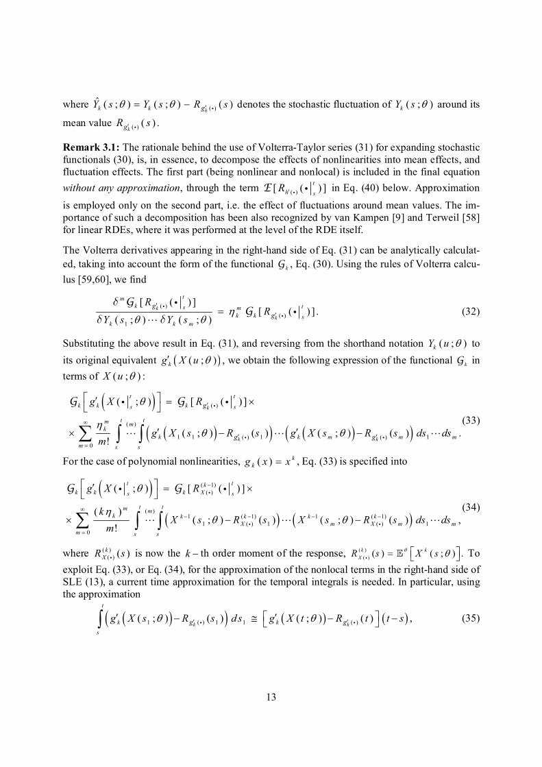
Remark 3.1: The rationale behind the use of Volterra-Taylor series (31) for expanding stochastic

functionals (30), is, in essence, to decompose the effects of nonlinearities into mean effects, and

fluctuation effects. The first part (being nonlinear and nonlocal) is included in the final equation

without any approximation, through the term ( )

[ ( ) ]t

h sR i iE in Eq. (40) below. Approximation

is employed only on the second part, i.e. the effect of fluctuations around mean values. The im-

portance of such a decomposition has been also recognized by van Kampen [9] and Terweil [58]

for linear RDEs, where it was performed at the level of the RDE itself.

The Volterra derivatives appearing in the right-hand side of Eq. (31) can be analytically calculat-

ed, taking into account the form of the functional k

G , Eq. (30). Using the rules of Volterra calcu-

lus [59,60], we find

( )

( )

1

[ ( ) ][ ( ) ]

( ; ) ( ; )

k

k

tm

k ts m

k k s

k k m

g

g

RR

Y s Y s

i

i

ii

⋯

GG

δ

δ δ. (32)

Substituting the above result in Eq. (31), and reversing from the shorthand notation ( ; )kY u to

its original equivalent ( ; )kg X u , we obtain the following expression of the functional k

G in

terms of ( ; )X u :

( )

( )

1 1 1 1( ) ( )

0

( ; ) [ ( ) ]

( ; ) ( ) ( ; ) ( ) .!

k

k k

t t

k k ks s

t tm mk

k k m m m

m s s

g

g g

g X R

g X s R s g X s R s ds dsm

i

i i

i i

⋯ ⋯ ⋯

G G

(33)

For the case of polynomial nonlinearities, ( ) k

kg x x , Eq. (33) is specified into

( 1)

( )

( )1 ( 1) 1 ( 1)

1 ( ) 1 ( ) 1

0

( ; ) [ ( ) ]

( )( ; ) ( ) ( ; ) ( ) ,

!

t tk

k k k Xs s

t tm mk k k k k

X m X m m

m s s

g X R

kX s R s X s R s ds ds

m

i

i i

i i

⋯ ⋯ ⋯

G G

(34)

where ( )

( ) ( )k

XR si is now the k th order moment of the response, ( )

( )( ) ( ; ) .

k k

XR s X s

iE To

exploit Eq. (33), or Eq. (34), for the approximation of the nonlocal terms in the right-hand side of

SLE (13), a current time approximation for the temporal integrals is needed. In particular, using

the approximation

1 1 1( ) ( )( ; ) ( ) ( ; ) ( )k k

t

k k

s

g gg X s R s d s g X t R t t s i i, (35)

14

and similarly for the other integrals(5), we obtain

( )

0

1( ; ) [ ( ) ] ( ; ) ( )

!k

t t m m

k k k ks s

m

gg X R X t t sm

i

i iG G , (36)

where

( ) ( )( , ) ; ( ) ( ) ( )k kk k k kg gx t x R t g x R t i i

. (6) (37)

Note that, contrary to SCT and Fox’s current time approximations, Eqs. (20), (24), current time

approximation (35) is applied to integrals of the fluctuations ( )( ; ) ( )kk gg X t R t i of random

functions ( ; )kg X t around their mean values, and not to the random functions per se. This

fact makes Eq. (35) a more accurate current time approximation. By substituting Eq. (36) into Eq.

(29), we obtain the approximation

1 ( )

2

02

exp [ ( ; ) ] exp ( ) ( )

1( ; ) , ( ) .

!

k

tNt

h ks

k s

N

m m

k

mk

gX t s R u du

X t t t sm

iiI

(38)

The exponential term, in the right-hand side of Eq. (38), is identified (via Eq. (28)) as the expres-

sion exp ( ; )t

s

h X u du E and is denoted, for simplicity, by ( )

[ ( ) ]t

h sR i iE . That is,

( ) 1 ( )

2

[ ( ) ] exp ( ; ) exp ( ) ( ) ,k

t tNt

h ks

ks s

gR h X u du t s R u du

i ii EE

(39)

where ( )( ) ( ; )

hR u h X u i

E . Since the series in the right-hand side of Eq. (38) are ab-

solutely convergent, use of the Cauchy product for the multiplication of more than two series

leads to the following, more convenient, equivalent form:

( )

1 | |

( ; ) ,exp [ ( ; ) ] [ ( ) ] 1 ( )

!

t t m

h hs s

m m

X t tX R t s

α

α

φ

αi

i iI E , (40)

where 2( , ) ( , ) , , ( , )Nx t x t x t φ and 2( , , )N α is a multi-index. Recall that,

2| |

Na a α ⋯ , 2

2( , ) ( , ) ( , )Na a

Nx t x t x t α

φ ⋯ and 2! ( !) ( !)Na aα ⋯ .

The right-hand side of approximation (40) contains two factors; the first one, ( )[ ( ) ]

t

h sR i iE , is a

functional on the response moments over time history, while the second is a sum encapsulating

(5) Note that the multiple integrals in Eqs. (33) and (34) can be written as products of single ones.

(6) Both notations, ( , )k

x t and ( )

( ; ( ) )kk g

x R t i will be used subsequently. The former in the derivation pro-

cedure and the latter in the final form of genFPK equations, to make clear the dependencies.

15

the effect of fluctuations of the nonlinear terms around the said moments. Thus, approximation

(40) retains a certain amount of nonlocality, through the term ( )[ ( ) ]

t

h sR i iE , a feature that con-

stitutes the main difference between the present method and the existing ones (Fox’s and SCT).

By truncating the series in Eq. (40) at a finite m M , and substituting it in SLE (13), we obtain

the following novel genFPK equation

0 0

( )

( ) ( )

2( )eff eff

0 ( ) ( ) ( )2

1 | |

( )( ) ( ) ( )

; { ( )}( ) , ( ) , ( ) ,

!

k

X t

X t

Mt t

h m h X tt t

m m

g

f xh x m t f x

t x

x R tD R t D R t f x

x

α

α

φ

α

i

i

i ii i

(41)

in which coefficients eff ( )mD t , called the generalized effective noise intensities, are given by

0 0

0

0 ( )

eff

( ) ( ) 0

2

( ) ( ) ( )

([ ( ) , ] [ ( ) ] ( )

[ ( ) ] )

)

( , ( ) ,

t t m

m h ht t

t

t

X

m

h s

t

D R t R t t

R C t s t s d

C

s

t

ii i

i i i

i i

i

E

E (42)

and

2

2( ) ( ) ( ); { ( )} ; ( ) , , ; ( )

k NNg g gx R t x R t x R t φ

i i i. (43)

Remark 3.2: Recalling Eq. (37), we observe that the x dependence of the terms

( ); ( )k

k gx R t i reflects the effects of the nonlinearities of the RDE, while the dependence on

( ) ( )k

gR t i introduces a new type local probabilistic nonlinearity, since moment ( ) ( )

kgR t i de-

pends on the unknown response pdf ( ) ( )X tf x at the current time t .

Remark 3.3: The dependence of eff

mD on 0

( )[ ( ) ]

t

h tR i iE gives rise to a nonlocal probabilistic

nonlinearity, since it involves the time history of ( ) ( )Xf xi

, from 0t up to the current time t .

Taking into account Remarks 3.1 and 3.2, and defining | | 0

/ ! 1

α

α

φ α , the Xf dependent dif-

fusion coefficient in VADA, Eq. (41), can be written in the following concise form

( )eff

( )

0 | |

; ( )[ ; , ] ( ) ,

!

MX t

X m X

m m

x ff x t D f t

α

α

φ

αi

iiB . (44)

The probabilistic nonlocality and nonlinearity appearing through [ ; , ]Xf x tB are inherited from

the nonlocal term of the SLE, Eq. (4). The absence of such terms in the classical FPK equation is

due to the fact that the nonlocal term of the SLE is fully localized in the case of white noise exci-

16

tation; see Sec. 2(a). We thus conclude that VADA approach retains an amount of the original

nonlocality and nonlinearity of the SLE, albeit of a tractable nature, through the history and the

current-time values of certain response moments(7).

Equations of FPK type whose coefficients depend on the unknown pdf arise in many fields of

physics, e.g. in quantum systems [61,62], in problems with anomalous diffusion [63], in non-equilibrium thermodynamics [64] or in systems with long-range interactions [65]. A survey of

such equations, commonly called nonlinear FPK equations, is presented in the book [49].

Remark 3.4: Another important observation, concerning our main new result, Eq. (41), is the

following. If we keep only the zeroth-order term 0

eff

0 ( )[ ( ) , ]

t

h tD R t i i in the diffusion coefficient,

Eq. (41) reduces to the time-dependent genFPK equation derived by using Hänggi’s ansatz, also called the decoupling approximation, see e.g. [8, Eq. 5.17,27,28]. Thus, our approach systematiz-

es and generalizes Hänggi’s decoupling approximation, using Volterra-Taylor series. This fact justifies the name Volterra adjustable decoupling approximation (VADA), coined by the present

authors. Note that such a generalization of Hänggi’s ansatz (without increasing the order of

x derivatives in the genFPK equation), was deemed not possible by Hänggi himself; see [8] p.

273.

4. First numerical results

In order to quantify the range of validity and assess the accuracy of the novel genFPK equations

proposed in this work, a number of numerical simulations has been performed and briefly pre-

sented in this section. The numerical method used for solving the various versions of genFPK

equations employs: i) a partition of unity finite element method (PUFEM) for the discretization

of ( ) ( )X tf x in the state space [66], ii) a Bubnov-Galerkin technique for deriving ODEs govern-

ing the evolution of ( ) ( )X tf x , and iii) a Crank-Nicolson scheme for solving the said ODEs in the

time domain. A brief description of the numerical scheme is given in Appendix C in ESM. Simi-lar numerical methods have been used for solving the standard FPK equation by Kumar and co-

workers [67,68]. This approach, being free of the burden of inter-element continuity/smoothness problems (because of the use of partition of unity), seems promising for extension to higher di-

mensions, and a first step towards this goal has been taken by Sun and Kumar in [69] for the clas-sical FPK equation.

A feature peculiar to our novel genFPK equations, calling for special numerical treatment, is their

nonlinear/nonlocal character. This peculiarity is treated by a self-contained, iterative scheme as follows: the current-time values of the response moments, needed for the calculation of diffusion

coefficient [ ; , ]Xf x tB , are estimated by extrapolation based on the two previous time steps,

and then are improved by iterations at the current time. Usually one or two iterations suffice. The final values of these moments, for each time instant, are stored and used for the calculation of the

nonlocal terms (time integrals) in eff

mD , as required by Eqs. (39) and (42). A more detailed de-

scription of the numerical scheme is given in Appendix C in ESM.

(7) Which are dictated by the structure of nonlinearity of the corresponding RDE.

17

The numerical results to be presented subsequently concern the response pdf of the nonlinear,

bistable RDE

3

1 3( ; ) ( ; ) ( ; ) ( ; )X t X t X t t ɺ , 0 0( ; ) ( )X t X , (45a,b)

with 1 0 ,

3 0 . For this case, the excitation is considered a zero-mean OU process, and the

initial value 0 ( )X is taken uncorrelated to the excitation. Then, by introducing the dimension-

less variables [8] 1t tɶ ,

3 1| | /X X ɶ ,

0 0 3 1| | /X X ɶ and 3

3 1| | / ɶ , RDE

(45) is expressed as

3( ; ) ( ; ) ( ; ) ( ; )X t X t X t t ɺɶ ɶ ɶ ɶɶ ɶ ɶ ɶ , 0 0( ; ) ( )X t X ɶ ɶɶ . (46a,b)

Furthermore, the determination of autocorrelation function of the normalized ( ; )t ɶ ɶ calls for

the normalization of the correlation time cor and intensity

OUD of OU noise excitation. For this

purpose, the relaxation time rel of the homogeneous variant ( ( ; ) 0t ) of Eq. (45) is chosen

as reference time. Since homogeneous Eq. (45) is a Bernoulli equation, its relaxation time is

found to be rel 11/ (2 ) (by studying the long-time behaviour of analytic solution). Thus, the

dimensionless correlation time, called also relative correlation time, is defined as

cor rel 1 cor/ 2 ɶ . (47)

On the basis of Eq. (47) and the definition of the normalized excitation ( ; )t ɶ ɶ , the autocorrela-

tion function of the latter is expressed as

( ) ( )

2 | |( , ) exp

D t sC t s

ɶ ɶi i

ɶ ɶ ɶɶ ɶ

ɶ ɶ, (48)

with dimensionless intensity

32

O U 2

1

| |2D D

ɶ . (49)

As an example, we consider the dimensionless RDE (46) with 1D ɶ , and ɶ taking values in the

range 0.1 3.0 . That is, we study a strongly nonlinear, bistable case, under strong random exci-

tation outside of the small-noise intensity regime [8,34], over a wide range of relative correlation

times. Initial pdf is taken to be Gaussian with zero mean value and variance 0.6 . In Figure 1

we present the evolution of the response pdf for increasing values of the ratio cor rel/ ɶ , as

calculated by solving the genFPK equations based on:

Small correlation time approximation, Eq. (21) (SCT),

0th-order VADA (Hänggi’s ansatz), Eq. (41) with 0M (HAN),

2nd

-order VADA, Eq. (41) with 2M (VADA-II) and

4th-order VADA, Eq. (41) with 4M (VADA-IV).

In the same figure, results obtained by Monte Carlo (MC) simulations are plotted, denoted by sim

in the legends, for comparison purposes. The choice of even order VADA genFPK equations is

made in order to ensure the global positivity of the corresponding diffusion coefficients.

18

Figure 1. Evolution of response pdf for the RDE (46) excited by a zero-mean OU process with

1D and 0.1, 0.3, 0.5,1.0,1.5, 3.0 . Initial pdf is zero-mean Gaussian with 0.6 . Re-

sults from various methods are presented along with MC simulations (coloured online).

19

Note that the final time instant in all plots is chosen to be in the long-time stationary regime, in

order to check the validity of genFPK equations in both the transient and the stationary regimes.

As shown in the figure, for small values of (Fig. 1a, cor rel/ 0.1 )(8), all methods work

well, with SCT and VADAs predicting a time evolution of response pdf in full agreement with

MC simulations, both in the transient and the steady state regime. Only HAN slightly underesti-

mates the peak values of the stationary pdf. As increases (Fig. 1b, 0.3 ) SCT is absent

since the increase of renders its diffusion coefficient negative (and the SCT approximation in-valid). HAN underestimates the pdf peak values more, while both VADA-II and IV are in almost

full agreement with MC simulations. This picture is practically the same in Fig. 1c ( 0.5 ),

with HAN being even worse. For larger values of (Fig. 1d, 1 ), both VADAs are fairly ac-

curate; however, they are a bit off at the peak values of the stationary pdf. For even larger values

of (Fig. 1e, 1.5 and Fig. 1f, 3 ) HAN fails totally, while VADA-II and IV provide fairly

accurate approximations, except for a minor failure at predicting the pdf peak values. Besides, the abscissae of the peak values predicted by VADAs are somewhat shifted closer to zero, in com-

parison with the ones of the MC results. In Appendix D in ESM, where a more detailed investiga-tion of parameters is performed, it is shown that VADA-II and IV continue to give acceptable

approximations of the pdf up to 5D and 5 , with slightly but constantly increasing errors.

As D and increase further, the problem becomes more difficult to solve numerically; the nu-merical scheme, in its present form, exhibits instabilities or divergence towards the end of the

transient state for various cases where 25D . The numerical solution of VADA-IV fails earli-

er than VADA-II (and HAN). This is reasonable, since higher-order polynomial terms are includ-

ed in VADA-IV, amplifying any instabilities in the numerical scheme.

Remark 4.1: An interesting phenomenon observed in both Fig. 1 above and in Figs. 4a,b of Ap-

pendix D is that, for large values of D and , the response pdfs of RDE (46), obtained by MC

simulations, exhibit their peak values at abscissae with absolute values larger than 1. This peak

value drift, which has been documented before, see e.g. [8] p. 294, is predicted quite accurately

by VADAs in the regime of ( , ) [0, 5.0] [0, 5.0]D , and -more generally- for 25D .

VADA-IV is consistently more accurate than VADA-II. Note that this this peak value drift is not

captured at all by HAN approach, which predicts pdfs with peaks fixed at 1 .

5. Conclusions and discussion

In the present work, we have developed a novel, efficient and accurate family of evolution equa-

tions governing the response pdf of a nonlinear scalar RDE, excited by coloured, Gaussian, addi-

tive noise. The excitation may have non-zero mean, and can be correlated with the initial state.

The genFPK equations obtained are valid in both the transient and the stationary regimes, as well

as for large correlation times and large noise intensities. What is more, their numerical solution,

e.g. by using the PUFEM method, requires comparable computational effort with the correspond-

ing classical FPK equation with the same state variables. Numerical results for a specific nonline-

ar bistable RDE confirm the validity and the accuracy of the proposed new genFPK equations.

(8) From now on (in the text and in figures’ captions) we omit the tilde from the non-dimensional quantities.

20

The derivation of the said new genFPK equations is made by elaborating the nonlocal term of the

stochastic Liouville equations using: i) a new extended form of the Novikov-Furutsu theorem, ii)

an approximation of the random nonlinear terms around their instantaneous moments, and iii) an

expansion of the memory terms around current time. The obtained genFPK equations are nonlin-

ear and nonlocal, yet easy to solve numerically. Also, they are able to rederive almost all existing

genFPK equations (for additive coloured noise excitation) with appropriate simplifications of

their terms. The approach presented herein has been called Volterra Adjustable Decoupling Ap-

proximation.

Finally, the present approach can be extended to systems of nonlinear RDEs under additive, col-

oured, Gaussian excitation. This direction is currently under consideration by the authors, and

some first results were recently presented in [42]. More specifically, in [42], the multidimension-

al counterpart of SLE (13) is derived. In the multidimensional SLE, the nonlocal term -analogous

to the nonlocal exponential term in SLE (13)- is identified as the transition matrix of the varia-

tional problem associated with the RDEs system. Subsequently, by appropriate approximations,

we are able to easily re-derive the usual multidimensional genFPK equation, for additive noise

excitation, found in the literature, see e.g. [70], as well as the multidimensional counterparts of

Fox’s genFPK equation, and Hänggi’s ansatz, which to the best of our knowledge, have not been

presented before. Multidimensional VADA genFPK equations have been also derived and will be

submitted for publication soon. Apart from this, extension to multiplicative coloured noise excita-

tion is possible, and it is under way, as well.

Acknowledgements. K.I. Mamis is supported by the ELKE-NTUA scholarship programme.

References

[1] R.L. Stratonovich, Some Markov methods in the theory of stochastic processes in nonlinear dynamical

systems, in: F. Moss, P.V.E. McClintock (Eds.), Noise Nonlinear Dyn. Syst. Vol. 1 Theory Contin. Fokker-Planck Syst., Cambridge University Press, 1989: pp. 16–71.

[2] C. Soize, The Fokker-Planck equation for stochastic dynamical systems and its explicit steady state

solutions, World Scientific, 1994. [3] H. Risken, The Fokker-Planck Equation. Methods of Solution and Applications, 2nd ed., Springer-Verlag,

1996.

[4] V.S. Pugachev, I.N. Sinitsyn, Stochastic Systems. Theory and Applications, World Scientific, 2001.

[5] C.W. Gardiner, Handbook of Stochastic Methods for Physics, Chemistry and the Natural Sciences, 3rd ed., Springer, 2004.

[6] J.Q. Sun, Stochastic Dynamics and Control, Elsevier, 2006.

[7] M.O. Cáceres, Non-equilibrium Statistical Physics with Application to Disordered Systems, Springer, 2017.

[8] P. Hänggi, P. Jung, Colored Noise in Dynamical Systems, Adv. Chem. Phys. 89 (1995) 239–326. [9] N.G. van Kampen, Stochastic Processes in Physics and Chemistry, 3rd ed., North Holland, 2007.

[10] T.P. Sapsis, G.A. Athanassoulis, New partial differential equations governing the joint, response-excitation, probability distributions of nonlinear systems, under general stochastic excitation, Probabilistic Eng. Mech. 23 (2008) 289–306. doi:10.1016/j.probengmech.2007.12.028.

[11] D. Venturi, T.P. Sapsis, H. Cho, G.E. Karniadakis, A computable evolution equation for the joint response-

excitation probability density function of stochastic dynamical systems, Proc.R.Soc.A. 468 (2012) 759–783.

[12] K. Wen, F. Sakata, Z.X. Li, X.Z. Wu, Y.X. Zhang, S.G. Zhou, Non-Gaussian fluctuations and non-Markovian effects in the nuclear fusion process: Langevin dynamics emerging from quantum molecular

dynamics simulations, Phys. Rev. Lett. 111 (2013) 1–5. doi:10.1103/PhysRevLett.111.012501.

[13] G.A. Athanassoulis, I.C. Tsantili, Z.G. Kapelonis, Beyond the Markovian assumption: response-excitation probabilistic solution to random nonlinear differential equations in the long time, Proc.R.Soc.A. 471: (2015).

21

[14] J.I. Costa-Filho, R.B.B. Lima, R.R. Paiva, P.M. Soares, W.A.M. Morgado, R. Lo Franco, D.O. Soares-Pinto,

Enabling quantum non-Markovian dynamics by injection of classical colored noise, Phys. Rev. A. 95 (2017)

1–13. doi:10.1103/PhysRevA.95.052126. [15] I. De Vega, D. Alonso, Dynamics of non-Markovian open quantum systems, Rev. Mod. Phys. 89 (2017) 1–

58. doi:10.1103/RevModPhys.89.015001.

[16] T. Spanio, J. Hidalgo, M.A. Muñoz, Impact of environmental colored noise in single-species population dynamics, Phys. Rev. E. 96 (2017) 1–9. doi:10.1103/PhysRevE.96.042301.

[17] A. Francescutto, S. Naito, Large amplitude rolling in a realistic sea, Int. Shipbuild. Prog. 51 (2004) 221–235.

http://iospress.metapress.com/index/D58TRBX995AFJRJL.pdf.

[18] W. Chai, A. Naess, B.J. Leira, Filter models for prediction of stochastic ship roll response, Probabilistic Eng. Mech. 41 (2015) 104–114. doi:10.1016/j.probengmech.2015.06.002.

[19] P. Krée, Markovianization of Random Vibrations, in: L. Arnold, P. Kotelenez (Eds.), Stoch. Space-Time

Model. Limit Theorems, 1985: pp. 141–162.

[20] P. Hänggi, P. Jung, Dynamical systems: A unified colored-noise approximation, Phys. Rev. A. 35 (1987) 4464–4466.

[21] N.G. van Kampen, Remarks on Non-Markov Processes, Brazilian J. Phys. 28 (1998) 90–96.

[22] A.M. Cetto, L. de la Peña and R.M. Velasco Generalized Fokker-Planck Equations for Coloured, Multiplicative, Gaussian Noise, Rev. Mex. Física. 31 (1984) 83–101.

[23] N.G. van Kampen, Stochastic Differential Equations, Phys. Rep. 24 (1976) 171–228.

[24] R.F. Fox, Analysis of nonstationary Gaussian and non-Gaussian generalized Langevin equations using

methods of multiplicative stochastic processes, J. Stat. Phys. 16 (1977) 259–279. [25] P. Hänggi, Correlation functions and Masterequations of generalized (non-Markovian) Langevin equations,

Zeitschrift Fur Phys. B. 31 (1978) 407–416.

[26] J.M. Sancho, M. San Miguel, S.L. Katz, J.D. Gunton, Analytical and numerical studies of multiplicative

noise, Phys. Rev. A. 26 (1982) 1589–1609. [27] P. Hänggi, T.J. Mroczkowski, F. Moss, P.V.E. McClintock, Bistability driven by colored noise: Theory and

experiment, Phys. Rev. A. 32 (1985) 695–698. doi:10.1103/PhysRevA.32.695.

[28] R.F. Fox, Functional-calculus approach to stochastic differential equations, Phys. Rev. A. 33 (1986) 467–476.

[29] E. Peacock-López, B.J. West, K. Lindenberg, Relations among effective Fokker-Planck for systems driven

by colored noise, Phys. Rev. A. 37 (1988) 3530–3535.

[30] R.L. Harne, K.W. Wang, Prospects for Nonlinear Energy Harvesting Systems Designed Near the Elastic Stability Limit When Driven by Colored Noise, J. Vib. Acoust. 136 (2014) 021009. doi:10.1115/1.4026212.

[31] M.F. Daqaq, Transduction of a bistable inductive generator driven by white and exponentially correlated Gaussian noise, J. Sound Vib. 330 (2011) 2554–2564. doi:10.1016/j.jsv.2010.12.005.

[32] P. Zhu, Y.J. Zhu, Statistical Properties of Intensity Fluctuation of Saturation Laser Model Driven By Cross-

Correlated Additive and Multiplicative Noises, Int. J. Mod. Phys. B. 24 (2010) 2175–2188.

doi:10.1142/S0217979210055755.

[33] H. Zhang, T. Yang, W. Xu, Y. Xu, Effects of non-Gaussian noise on logical stochastic resonance in a triple-well potential system, Nonlinear Dyn. 76 (2014) 649–656. doi:10.1007/s11071-013-1158-3.

[34] L. Ridolfi, P. D’Odorico, F. Lalo, Noise-Induced Phenomena in the Environmental Sciences, Cambridge

University Press, 2011. [35] C. Zeng, Q. Xie, T. Wang, C. Zhang, X. Dong, L. Guan, K. Li, W. Duan, Stochastic ecological kinetics of

regime shifts in a time-delayed lake eutrophication ecosystem, Ecosphere. 8 (2017). doi:10.1002/ecs2.1805.

[36] C. Zeng, H. Wang, Colored Noise Enhanced Stability in a Tumor Cell Growth System Under Immune Response, J. Stat. Phys. 141 (2010) 889–908. doi:10.1007/s10955-010-0068-8.

[37] T. Yang, Q.L. Han, C.H. Zeng, H. Wang, Z.Q. Liu, C. Zhang, D. Tian, Transition and resonance induced by

colored noises in tumor model under immune surveillance, Indian J. Phys. 88 (2014) 1211–1219.

doi:10.1007/s12648-014-0521-7.

[38] P. Hänggi, Colored noise in continuous dynamical systems: a functional calculus approach, in: F. Moss, P.V.E. McClintock (Eds.), Noise Nonlinear Dyn. Syst. Vol. 1 Theory Contin. Fokker-Planck Syst.,

Cambridge University Press, 1989: pp. 307–328.

[39] J.M. Sancho, M. San Miguel, Langevin equations with colored noise, in: F. Moss, P.V.E. McClintock (Eds.), Noise Nonlinear Dyn. Syst. Vol. 1 Theory Contin. Fokker-Planck Syst., Cambridge University Press, 1989:

pp. 72–109.

[40] J.B.T.M. Roerdink, Inhomogeneous linear random differential equations with mutual correlations between

22

multiplicative, additive and initial-value terms, Physica. 109A (1981) 23–57.

[41] J.B.T.M. Roerdink, A cumulant expansion for the time correlation functions of solutions to linear stochastic

differential equations, Physica. 112A (1982) 557–587. [42] K.I. Mamis, G.A. Athanassoulis, K.E. Papadopoulos, Generalized FPK equations corresponding to systems

of nonlinear random differential equations excited by colored noise. Revisitation and new directions,

Procedia Comput. Sci. 136 (2018) 164–173. [43] J.M. Sancho, M. San Miguel, External non-white noise and nonequilibrium phase transitions, Zeitschrift Fur

Phys. B. 36 (1980) 357–364.

[44] P. Wang, A.M. Tartakovsky, D.M. Tartakovsky, Probability density function method for langevin equations

with colored noise, Phys. Rev. Lett. 110 (2013) 1–4. doi:10.1103/PhysRevLett.110.140602. [45] T.S. Lundgren, Distribution functions in the statistical theory of turbulence, Phys. Fluids. 10 (1967) 969–

975.

[46] S.B. Pope, Pdf methods for turbulent reactive flows, Prog. Energy Combust. 11 (1985).

[47] N.G. van Kampen, Stochastic Differential Equations, in: E.G.D. Cohen (Ed.), Fundam. Probl. Stat. Mech. III, North-Holland, 1975: pp. 257–276.

[48] G.A. Athanassoulis, K.I. Mamis, Extensions of the Novikov-Furutsu theorem, obtained by using Volterra

functional calculus, Phys. Scr. in press (2019). doi:10.1088/1402-4896/ab10b5. [49] T.D. Frank, Nonlinear Fokker-Planck Equations, Springer, 2005.

[50] D. V. Anosov, V.I. Arnold, eds., Dynamical Systems I, Springer-Verlag, 1987.

[51] H. Amann, Ordinary Differential Equations, Walter de Gruyter, 1990.

[52] A. Grigorian, Ordinary Differential Equation (Lecture Notes), University of Bielefeld, 2008. [53] R.F. Fox, Stochastic calculus in physics, J. Stat. Phys. 46 (1987) 1145–1157. doi:10.1007/BF01011160. [54] W. Cheney, W. Light, A Course in Approximation theory, American Mathematical Society, 2009.

[55] N. Bandyopadhyay, Physical Mathematics, Academic Publishers, 2002.

[56] J.F. Barrett, The use of characteristic functionals and cumulant-generating functionals to discuss the effect of noise in linear systems, J. Sound Vib. 1 (1964) 229–238.

[57] M.O. Cáceres, Harmonic potential driven by long-range correlated noise, Phys. Rev. E. 60 (1999) 5208–

5217. [58] R.H. Terwiel, Projection operator method applied to stochastic linear differential equations, Physica. 74

(1974) 248–265.

[59] V.I. Averbukh, O.G. Smolyanov, The various definitions of the derivative in linear topological spaces, Russ.

Math. Surv. 23 (1968) 67–113. [60] V. Volterra, Theory of Functionals and of Integral and Integro-differential Equations, Phoenix, Dover

Publications (2005 reprint), 1930. [61] J.A. Carrillo, J. Rosado, F. Salvarani, 1D nonlinear Fokker-Planck equations for fermions and bosons, Appl.

Math. Lett. 21 (2008) 148–154. doi:10.1016/j.aml.2006.06.023.

[62] A. Sakhnovich, L. Sakhnovich, The nonlinear Fokker-Planck equation: Comparison of the classical and

quantum (boson and fermion) characteristics, J. Phys. Conf. Ser. 343 (2012). doi:10.1088/1742-

6596/343/1/012108. [63] E.M.F. Curado, F.D. Nobre, Derivation of nonlinear Fokker-Planck equations by means of approximations to

the master equation, Phys. Rev. E - Stat. Physics, Plasmas, Fluids, Relat. Interdiscip. Top. 67 (2003) 7.

doi:10.1103/PhysRevE.67.021107. [64] T.D. Frank, Generalized Fokker-Planck equations derived from generalized linear nonequilibrium

thermodynamics, Phys. A Stat. Mech. Its Appl. 310 (2002) 397–412. doi:10.1016/S0378-4371(02)00821-X.

[65] A.A. Zaikin, L. Schimansky-Geier, Spatial patterns induced by additive noise, Phys. Rev. E. 58 (1998) 4355–4360.

[66] J.M. Melenk, I. Babuska, The partition of unity finite element method: Basic theory and applications,

Comput. Methods Appl. Mech. Eng. 139 (1996) 289–314.

[67] M. Kumar, S. Chakravorty, P. Singla, J.L. Junkins, The partition of unity finite element approach with hp-

refinement for the stationary Fokker–Planck equation, J. Sound Vib. 327 (2009) 144–162. [68] M. Kumar, S. Chakravorty, J.L. Junkins, A semianalytic meshless approach to the transient Fokker-Planck

equation, Probabilistic Eng. Mech. 25 (2010) 323–331.

[69] Y. Sun, M. Kumar, A numerical solver for high dimensional transient Fokker-Planck equation in modeling polymeric fluids, J. Comput. Phys. 289 (2015) 149–168. doi:10.1016/j.jcp.2015.02.026.

[70] L. Garrido, J.M. Sancho, Ordered cumulant technique and differential equations for probability density,

Physica A. 115 (1982) 479–489.

23

[71] L. Arnold, Random Dynamical Systems, Springer, 1998.

[72] R. Kubo, Stochastic Liouville Equations, J. Math. Phys. 4 (1963) 174–183.

24

Appendix A. Derivation of the stochastic Liouville equation via the delta projection method

The random initial-value problem (RIVP) considered in the present work, Eq. (1a,b), is repeated

here for easy reference:

( ; ) ( ( ; ) ) ( ; )X t h X t t ɺ , (A1a)

0 0( ; ) ( )X t X . (A1b)

The random data of the RIVP (A1) are the initial value 0

( )X and the excitation ( ; )t , fully

described by the infinite-dimensional joint probability measure 0 ( )X iP , which is assumed to pos-

sess a well-defined probability density functional. The data measure 0 ( )X iP is considered de-

fined over the Borel algebra of the product space •ℝ , where • is with the space of

continuous functions 0[ , ]C t t ℝ . The marginal data measure

( ) iP is assumed to have con-

tinuous mean value and autocovariance operators (and thus continuous two-point correlation

functions), reflecting the colored-noise character of the excitation ( ; )t . The complete proba-

bilistic solution of the RIVP (A1) is described by the joint response-excitation probability meas-

ure ( ) ( )X i i

P , which is assumed to exist and possess a joint probability density functional (and

thus, finite-dimensional pdfs of all orders). It is assumed that the solution measure ( ) ( )X i i

P is

defined over the Borel algebra of the product space X • , where • is the same as

above, and X coincides with the space 1

0[ , ]C t t ℝ , in which the response path functions

belong. In addition, the solution measure ( ) ( )X i i

P must obey the compatibility condition that its

marginal measure 0( ) ( )X t iP is equal to the given data measure

0 ( )X iP . Having assumed that the

underlying infinite-dimensional (measure) problem is well-posed, we focus on a systematic deri-

vation of solvable approximate equations governing the evolution of the one-time response pdf

( ) ( )X tf x . Note that the response process ( ; )X t is non-Markovian, since the excitation

( ; )t is colored, and non-Gaussian when the system function ( )h x is nonlinear.

(a) Delta projection method

Representing the one-time pdf of a random function as the average of a random delta function,

( ) ( ) ( ( ; ) )X tf x x X t , (A2)

where i is an appropriate ensemble average operator, widely-used practice in statistical me-

chanics (van Kampen, 2007, chap. XVI, sec.5), stochastic dynamics (Venturi et al., 2012), and

the theory of turbulence (Lundgren, 1967), where it is called the pdf method. Herein, the more

suggestive term delta projection method is employed. In this subsection we (re)derive formula

(A2) in a more generic way, obtaining also some generalizations of it which are useful in deriving

the stochastic Liouville equation (SLE) corresponding to a nonlinear RDE.

25

To start with, we consider two integrable functions, 1 ( )g i , 2 ( )g i , and formulate the average of

the product 1 2( ; ) ( ; )g X g s , for some (fixed) 0

, [ , ]s t t :

( ) ( ) 1 2

1 2 ( ) ( )

( ; ) ( ; )

( ) ( ) ( ) ( ) .

X

X

g X g s

g g s d d

X •

i i

i ii i

P

P

E

(A3)

From now on the symbol ( ) ( )

[ ]X

i ii

PE , of the ensemble average operator with respect to the joint

response-excitation probability measure, is simplified to [ ]iE . Since the integrand in the right-

hand side of Eq. (A3) depends only on the specific values ( ) and ( )s of the path functions

( ) i and ( ) i , the infinite-dimensional integral is reduced to a two-dimensional one, with re-

spect to marginal, two-point measure ( ) ( )X s P :

21 2 1 2 ( ) ( )

( ; ) ( ; ) ( ) ( )X s

g X g s g w g z d w d z

ℝ PE ,

which is also written, using the joint pdf ( ) ( )

( , )X s

f w z , as

21 2 1 2 ( ) ( )

( ; ) ( ; ) ( ) ( ) ( , )X s

g X g s g w g z f w z d w d z

ℝE . (A4)

We shall now apply Eq. (A4) to cases where one of the two functions 1( )g i ,

2( )g i is a general-

ized function, namely the delta function or some derivative of it. Justification of this extension

can be made by invoking the theory of generalized stochastic processes; see e.g. (Gel’fand and

Vilenkin, 1964, chap. III). Following the tradition in statistical physics, we shall proceed formal-

ly, without performing rigorous proofs in the context of the theory of generalized stochastic pro-

cesses.

Setting 1 ( ; ) ( ( ; ) )g X t x X t and 2 ( ; ) 1g s in Eq. (A4), we obtain

2 ( ) ( )

( ) ( )

( ( ; ) ) ( ) ( , )

( ) ( ) ( ),

X t s

X t X t

x X t x w f w z d w d z

x w f w d w f x

ℝ

ℝ

E

(A5)

which is the same as Eq. (A2). Setting now

1

( ( ; ) )( ; ) ( ; )

( ; )

x X tg X t q X t

X t

and 2 ( ; ) 1g s ,

and assuming that the functions ( )q x and ( )( )

X tf x are continuously differentiable, Eq. (A4)

provides us with the formula

26

2 ( ) ( )

( )( ) ( , )

( ( ; ) )( ; )

( ; )X t s

x wq w f w z d w d z

w

x X tq X t

X t

ℝE

( )

( )( ) ( )

X t

x wq w f w d w

w

ℝ

( )( ) ( )X tq x f xx

. (A6)

By replacing, in the above equation, the first derivative of the delta function by its nth-derivative,

and working similarly as above, we obtain the following useful generalization of Eq. (A6):

( )

( ( ; ) )( ; ) ( 1) ( ) ( )

( ; )

n nn

X tn n

x X tq X t q x f x

X t x

E . (A7)

For Eq. (A7) to be valid, the functions ( )q x and ( )

( )X t

f x should possess nth-order continuous

derivatives. Finally, if we specify

1

( ( ; ) )( ; ) ( ; )

( ; )

n

n

x X tg X t q X t

X t

and 2 ( ; ) ( ; )g t t ,

and assume the same differentiability conditions on ( )q x and ( )

( )X t

f x as above, Eq. (A4) leads

to:

2 ( ) ( )

( ) ( )

( )( ) ( , )

( ( ; ) )( ; ) ( ; )

( ; )

( 1) ( ) ( , )

n

X t tn

n

n

nn

X t tn

x wq w z f w z d w d z

w

x X tq X t t

X t

q x z f x z d zx

ℝ

ℝ

E

( 1) ( ) ( ( ; ) ) ( ; ) .n

n

nq x x X t t

x

E (A8)

The last equality holds true since

2

( ) ( ) ( ) ( )( , ) ( ) ( , ) .X t t X t tz f x z d z z x w f w z dwd z ℝ ℝ

(b) Derivation of the stochastic Liouville equation

We shall now apply the delta projection method to derive an equation governing the evolution of

the response pdf ( )

( )X t

f x , when ( ; )X t satisfies RDE (A1a). By differentiating the first and

the last members of Eq. (A5) with the respect to time, we find

( )( ) ( ( ; ) )

( ( ; ) ) ( ; )( ; )

X tf x x X t

x X t X tt t X t

ɺE E . (A9)

27

The rightmost side of Eq. (A9) is derived by interchanging differentiation and expectation opera-

tors and using chain rule in differentiation. Now, in Eq. (A9), ( ; )X t ɺ is substituted via RDE

(A1a), leading to

( )( ) ( ( ; ) ) ( ( ; ) )

( ( ; ) ) ( ; )( ; ) ( ; )

X tf x x X t x X t

h X t tt X t X t

E E . (A10)

Reformulation of the averages in the right-hand side of Eq. (A10), using Eqs. (A6) with ( )q x

( )h x for the first term, and Eq. (A8) with 1n and ( ) 1q x for the second term, results in

( )

( )

( )( ) ( ) ( ; ) ( ( ; ) )

X t

X t

f xh x f x t x X t

t x x

E , (A11)

which is the stochastic Liouville equation (SLE), Eq. (3) of the main paper. This equation has

been derived by many authors, using various approaches; see e.g. (Hänggi, 1978; Sancho and San

Miguel, 1980; Sancho et al., 1982; Cetto et al., 1984; Fox, 1986; Venturi et al., 2012). Also, the

initial condition for SLE (A11) is easily determined, by use of Eq. (A5):

00 0 0( ) ( ( ; ) ) ( ( )( ) XX t x X t x X ff x E E . (A12)

In contrast with the classical Liouville equation (Schwabl, 2006, sec. 1.3.2), (van Kampen, 2007,

sec. XVI.5), the SLE (A11) is not closed, due to the averaged term

( ; ) ( ( ; ) )X t x X t N E , (A13)

appearing in its right-hand side. This fact is better illustrated if the right-hand side of Eq. (A11) is

rewritten as (see Eq. (8)):

( ) ( ) ( )

( )

( ) ( , )( ) ( )

X t X t t

X t

f x f x zh x f x z d z

t x x

ℝ

. (A14)

Eq. (A14) is clearly not closed, since, apart from ( ) ( )X tf x , it also contains the joint response-

excitation pdf ( ) ( ) ( , )X t tf x z . Some ideas for obtaining approximate closures of the above equa-

tion have been presented in (Venturi et al., 2012; Athanassoulis, Tsantili and Kapelonis, 2015).

Nevertheless, our goal in this work, as mentioned in the introduction, is to provide a closure for

the SLE in the form of Eq. (A11).

(c) Comparison of SLE derivation presented herein to van Kampen’s derivation

Another technique for deriving SLE (A11) is by means of the so-called van Kampen’s lemma;

see (van Kampen 1975, p.269; van Kampen 1976, p.209; van Kampen 2007, p.411). The philos-

ophy behind van Kampen’s derivation of the SLE, based on the classical Liouville equation, is

distinctively different from the one presented in the previous section, although it leads to the

same result.

28

Van Kampen’s derivation starts with a path-wise consideration of the given RDE. That is, the

equation:

( ) ( ( ) ) ( )X t h X t t ɺ , 0

0( )X t X , (A15a,b)

is considered for every value of the stochastic argument separately. In this setting, (A15a,b) is

a deterministic initial value problem. Then, the indicator function

( , ) ( )p x t x X t ,

satisfies the classical Liouville equation

( , )( ) ( ) ( , )

p x th x t p x t

t x

, (A16a)

0

0( , )p x t x X ; (A16b)

(see (Klyatskin, 2005), Sec. 2.1). Van Kampen does not follow a formal derivation as

Klyatskin’s, using instead physical arguments after interpreting ( , )p x t as a “flow” and Eq.

(A16a) as a conservation law. Although the argument of van Kampen is somewhat obscure, it can

be justified by considering ( , )p x t as a counter of values (outcomes) satisfying the condi-

tion ( ) ( ; )X t X t x (“flow of outcomes”).

By applying, on both Eqs. (A16a,b) the ensemble average operator i over all , we obtain:

( , )

( ) ( , ) ( ; ) ( , )p x t

h x p x t t p x tt x x

, (A17a)

0 0( , ) ( )p x t x X . (A17b)

The step that completes van Kampen’s derivation of the SLE, see Eqs. (A11), (A12), is the iden-

tification

( ) ( ) ( , )X tf x p x t . (A18)

Eq. (A18) constitutes the van Kampen’s lemma per se. In his works, (van Kampen, loc. cit.), van

Kampen proves Eq. (A18) by employing a conservation argument. Note that, if we accept

( ; )x X t as a generalized random function, then the justification of Eq. (A18) is straight-

forward, being a special case of Eq. (A4) of our approach:

( ) ( )( , ) ( ; ) ( ) ( )X t X tp x t x X t x u f u d u f x ℝ

. (A19)

From the above discussion, a remarkable conceptual difference between van Kampen’s Lemma

and Eq. (A19) is revealed: in the former approach, the delta function is always treated as a deter-

29

ministic function, with the probabilistic arguments being provided by the conservation law,

while, in the latter, the delta function is interpreted, from the very beginning, as a stochastic func-

tion, on which the standard mean-value operator is applied.

In conclusion, although both approaches are interesting, revealing different conceptual settings,

we come to believe that formula (A4), on which our approach is based, is an ample generalization

of van Kampen’s lemma, Eq. (A18), providing a rigorous and systematic way to treat various

types of averages occurring in the derivation of the SLE.

30

Appendix B. On the solvability of the genFPK equation corresponding to a linear RDE

In this appendix we study the solvability (uniqueness and existence of solution) of the exact

genFPK Eq. (18) of the main paper, governing the evolution of the one-time response pdf

( ) ( )X tf x of a linear RDE under additive, Gaussian, coloured excitation. This issue seems to be

trivial from the practical point of view, since in this case the response pdfs of all orders are known (Gaussian). Nevertheless, it is significant from the foundational point of view, since it en-

sures the well-posedness of a new equation, as well as its consistency with known results. In ad-dition, after its theoretical justification, this equation provides us with a useful benchmark case

for the assessment of the accuracy of the numerical methods for solving the various genFPK equations, as e.g. Eq. (21), (25) and (41) of the main paper, which are more complicated variants

of the same type, that is, advection-diffusion equations.

(a) Statement of the problem

To facilitate the reader, we start by giving a complete yet concise statement of what has been al-

ready proved in Sec. 2 of the main paper, concerning the exact genFPK Eq. (18).

Under the conditions that: i) the excitation ( ; )t is a smoothly correlated (coloured) Gaussian

process, with mean value ( ) ( )m t i and autocovariance ( ) ( ) ( , )C t s i i,

ii) the initial value 0 ( )X is a Gaussian random variable, with mean value 0X

m and variance

0 0 0

2

X X XC , and

iii) 0 ( )X and ( ; )t are jointly Gaussian with cross-covariance 0 ( ) ( )XC t i ,

the one-time response pdf ( )( , ) ( )X tf x t f x of the linear random initial-value problem

(RIVP):

1( ; ) ( ; ) ( ; )X t X t t ɺ , (B1a)

0 0( ; ) ( )X t X , (B1b)

satisfies the following initial-value problem (IVP) (of a partial differential equation):

2

1 ( ) 2

0

( , ) ( , )( ) ( , ) ( ) 0,

, ,

f x t f x tx m t f x t D t

t x x

t t x

i (B2a)

0 0( , ) ( )f x t f x given , (B2b)

where the coefficient eff( ) ( )D t D t (the effective noise intensity) is given by

0

0

0

1 1( ) ( )2

(( ) )) (( ) ( , )( )X

tt t t s

t

D t e e dC C st t s

i ii

. (B2c)

The IVP (B2) will be studied under the following plausible assumptions:

31

A1) The function ( , )x f x t belongs to 2 ( )C ℝ for each 0t t ,

The function ( , )t f x t belongs to 1

0( , )C t for each x ℝ ,

The function ( , ) ( , )x t f x t is jointly continuous on 0[ , )t ℝ ,

A2) The integrals ( ) ( , )J t f x t d x

,

( ) ( ) ( , )Xm t x f x t d x

i ,

2( ) ( , )I t f x t d x

and

2

( , )( )

f x tP t d x

x

are finite,

A3) 2| | ( , ) 0x f x t as | |x ,

A4) ( ) 0D t for 0t t .

A solution of the IVP (B2) satisfying the above assumptions is called a classical solution.

A first, straightforward consequence from Eq. (B2a) and the assumptions A1) and A2) is that the

integral ( )J t is an invariant of the motion, which implies that 0( ) ( ) 1J t J t , as it should be,

since ( , )f x t is a probability density function. To prove this assertion, we integrate Eq. (B2a)

over the real axis and observe that the quantities appearing as end terms in the integration by pats

tend to zero as | |x .

(b) Uniqueness of solution

Theorem 1 [Uniqueness of the classical solution]. The IVP (B2) has at most one solution satisfy-

ing the assumptions A1) – A4).

The main tool for proving Theorem 1 is the following

Lemma 1. Under the assumptions A1) – A3), the integrals ( )I t and ( )P t of every classical so-

lution of Eq. (B2a) satisfy the following identity, for any 0t t :

1

1 1( ) ( ) ( ) ( ) 0

2 2

dI t I t D t P t

dt . (B3)

Proof (of lemma): During the proof we simplify the notation, writing ( )m t instead of ( ) ( )m t i .

Multiplying both members of Eq. (B2a) by ( , )f x t and integrating over the whole x axis, we

obtain

2

1 2

( , ) ( , )( ) ( , ) ( ) ( , ) 0

f x t f x tx m t f x t D t f x t d x

t x x

.

(B4a)

All integrals appearing in the above equation are well defined on the basis of the stated assump-

tions. Eq. (B4a) is also written in the form

1 2 3( ) ( ) ( ) 0I t I t I t , (B4b)

where

32

2

1

( , ) 1( ) ( , ) ( , )

2

f x t dI t f x t d x f x t d x

t dt

, (B5a)

2 1

2

1 1

( ) ( ) ( , ) ( , )

( , ) ( ) ( , ) ( , )

I t x m t f x t f x t d xx

f x t d x x m t f x t f x t d xx

2

2

1 1

1 ( , )( , ) ( )

2

f x tf x t d x x m t d x

x

, (B5b)

2

3 2

( , )( ) ( ) ( , )

f x tI t D t f x t d x

x

. (B5c)

Making an integration by parts in the last integral of the rightmost member of Eq. (B5b) and the integral in the right-hand side of Eq. (B5c), and observing that the end terms appearing after this

integration by parts are zero because of the assumptions A1) – A3), we find

2

2

1 1

( , )( ) ( , )

f x tx m t d x f x t d x

x

, (B6a)

22

2

( , ) ( , )( , )

f x t f x tf x t d x d x

x x

. (B6b)

Substituting the results (B6a,b) into Eqs. (B5b,c) we get

2

2 1

1( ) ( , )

2I t f x t d x

(B7a)

and 2

3

( , )( ) ( )

f x tI t D t d x

x

. (B7b)

Using Eqs. (B5a) and (B7a,b), Eq. (B4b) takes the form

2

2 2

1

1 1 ( , )( , ) ( , ) ( ) 0,

2 2

d f x tf x t d x f x t d x D t d x

dt x

which is identical with Eq. (B3). This completes the proof of the lemma.

We now proceed to the

Proof of Theorem 1. Assume that the IVP (B2) has two solutions, (1) ( , )f x t and ( 2) ( , )f x t .

Then, their difference (1) (2)*( , ) ( , ) ( , )f x t f x t f x t satisfies Eq. (B2a) and the homogene-

ous initial condition *0( , ) 0f x t . The integrals *( )I t and *( )P t (that is, the integrals ( )I t

and ( )P t with f substituted by *f ) will satisfy identity (B3), which is now written in the form

33

* * *1( ) ( ) 2 ( ) ( )

dI t I t D t P t

dt ,

0t t . (B8)

Clearly,

* ( ) 0P t , *( ) 0I t and *0( ) 0I t . (B9a,b,c)

Considering Eq. (B8) as a differential equation with respect to *( )I t , with initial condition

(B9c), we obtain

0

* *1( ) 2 ( ) ( ) exp ( )

t

tI t D P t d . (B10)

Since ( ) 0D t and *( ) 0P t , Eq. (B10) tells us that *( ) 0I t . The latter inequality, in con-

junction with inequality (B9b), implies that

2* *( ) ( , ) 0I t f x t d x

.

Thus, * ( , ) 0f x t , which means that the two solutions, (1) ( , )f x t and (2) ( , )f x t are identical.

This completes the proof of uniqueness theorem.

(c) Existence of solution and consistency with known results

We start by invoking the well-known result, that the response process of any linear system to an

additive Gaussian excitation (either coloured or white) is also a Gaussian process. Thus, the re-

sponse pdf ( ) ( )X tf x of the linear RIVP (B1) is given by the formula

2

( )

( ) 22( )( )

1 1( ) exp

2 ( )2 ( )

( )X t

XX

Xx

t

mx

tf

t

i

ii

, (B11)

where ( ) ( )Xm ti is the mean value and

2

( ) ( )X ti is the variance of the response ( ; )X t . The

deterministic functions ( ) ( )Xm ti

and 2

( ) ( )X ti

are defined as solutions of the corresponding

moment equations which, in the present case, take the form (see e.g. (Sun, 2006) ch. 8, or

(Athanassoulis, Tsantili and Kapelonis, 2015)):

( ) 1 ( ) ( )( ) ( ) ( )X Xm t m t m t i i i

ɺ , 0( ) 0( )X Xm t mi, (B12a,b)

1 0

0

1

0

2 2

( ) ( ) ( )

(

( )

2

)

1

( )

( )

1( ) ( ) ( )

2

, ,

X X

t t

X

tt u

t

C t e

C u t e du

t t

i i i

i i

ɺ

(B13a)

0 0

2

( ) 0( ) XX Xt C i

. (B13b)

Observe that, because of Eq. (B2c), Eq. (B13a) can be equivalently written as

34

1

2 2

( ) ( )( )

1( )

2( )

X XD tt t

i iɺ . (B13a′)

Taking advantage of the above results, we shall now verify that the (unique) solution of the IVP (B2) is given by Eq. (B11). This establishes existence of solution, and consistency with existing

results.

In order to verify that the function ( ) ( )X tf x , as defined by Eq. (B11), satisfies the IVP (B2), the

temporal and spatial derivatives of it are needed. The calculation of these derivatives is straight-

forward (details are omitted). The useful results are collected below:

( ) 2

( ) ( ) ( )22

( )

( )( ) ; ( ) ,

((

)) ,

X t

X t X X

X

f xf x x

tt t

tm

i i

i

(B14)

( ) 2

( ) ( )22

( )

( )

( )( ) ; ( ) ,

( )( ) ,X

X t

X t X

X

f xf x x t

xm

tt

ii

i

(B15)

2( ) 2

( ) ( )22 2(

(

)

)

( )( ) ; ( ) ,

( )( ) ,

X

X

t

X t X

X

fm t

xf x x t

x t

ii

i

(B16)

where

2 2

( ) ( ) ( )

2 2

( ) ( )

2 2 2 2 2

( ) ( ) ( ) ( ) ( ) ( ) (

2

)

1( ) ,

2

( ) ( )

1 1( ) ( )

A ; ( ) ( )

( ) ( )

( ) ( ) ( ) ( ) ( )2

.2

X X X

X X X

X X X X X X

X

X

m t

m t m t

m t

x xt

m t

t

t t

m t t t t t

x

i i i

i i

i i i i i i i

ɺ

ɺ

ɺ ɺ

ɺ

ɺ

(B17)

(

2 2 2

( ) ( ) )) (( )( ) ,; ( ) ( ) )( ) (X XX X Xtm ttx x m tt ii i i i . (B18)

2 2

( ) (

2

( ) )( ( )

2

); ( ) , 2 ( ) ( )( ) ( )X XX X Xm t mt tx x m t tx i ii i i . (B19)

Using Eqs. (B14) - (B16), the genFPK (advection-diffusion) Eq. (B2a) takes the form

22

)1 1 (( )( ( ) () 0)X x m t Dt t ii . (B20)

Lemma 2: Eq. (B20) is satisfied for all x ℝ and 0t t if and only if the moment equations

(B12a) and ( B13 a ) are satisfied for all 0t t .

Proof: Substituting the expressions (B17) – (B19), for the quantities , , , into Eq (B20), and

grouping together the coefficients of the same powers of x , results in

35

2 2

( ) ( )

2 2 2

( ) ( ) ( )

2 2

( ) ( )

1

( ) ( ) ( ) 1

2

( ) ( ) ( )

2

( )

1( )

2

( ) ( ) ( ) 2 ( )

1( ) ( ) ( ) ( )

( ) ( )

( ) ( ) ( )

( ) (( )2

)

X X

X X XX X

X X XX X

D t

m t

t t

t t t

t

m t m t D t

D t m t m t

x

m m t t

x

t

i i

i i

i i i

i i

i

i i i i

ɺ

ɺ

ɺ

ɺ

ɺ

1

2 2 2

( ) ( ) ( )( )1

( )2

( ) ( ) 0.X X Xt t tD t

i i iɺ (B21)

This means that Eq. (B20) will be satisfied for all x ℝ and 0t t if and only if the (three) co-

efficients of 2x , x and 0x (the x independent term), in Eq. (B21), are zero for all 0 .t t We

shall now show that the latter condition is equivalent with the satisfaction of the two moment

equations (B12a) and ( B13 a ) .

Assume that Eqs. (B12a) and ( B13 a ) are satisfied. Then, the coefficient of 2x in Eq.

(B21) becomes zero, and the same happens with the last term of the coefficient of 0x . By substi-

tuting 2 2

( ) (1 )( ) 2 2 ( )( )X X tt t D i i

ɺ , from Eq. ( B13 a ) , in the coefficient of x , we obtain

Coeff. of x = ( )( )

2

) 1 ( ( )(( ) ) ( ) ( )XX Xt m t m t m t i i iiɺ , (B22)

which vanishes because of Eq. (B12a). Finally, making the same substitution of 2

( ) ( )X ti

ɺ into the

remaining part of the x independent term, in Eq. (B21), we find

Coeff. of 0x = 2

( )1 ( ) ( ) ( ) ( )( ) ( ) ( ) ( ) ( )X X X Xm t m t m t m t t i i ii i

ɺ , (B23)

which also vanishes because of Eq. (B12a). This completes the proof that, if Eqs. (B12a) and

( B13 a ) are satisfied, then the coefficients of 2x , x and 0x , in Eq. (B21), are zero and thus Eq.

(B21) becomes an identity.

Assume now that the three coefficients of 2x , x and 0x , in Eq. (B21), are zero. From the coeffi-

cient of 2x we obtain Eq. ( B13 a ) . Using the latter, we transform the coefficient of x in the

form of Eq. (B22), from which we conclude that Eq. (B12a) is also satisfied. Finally, the coeffi-

cients of 0x takes again the form (B23), being zero without providing any new information. The

proof of Lemma 2 is completed.

Theorem 2 [Existence and consistency of solution]. The unique solution of the IVP (B2) is given

by the Gaussian pdf, Eq. (B11).

Proof: According to Lemma 2, and the discussion preceding it, the function ( ) ( )X tf x , as defined

by Eq. (B11), with mean value ( ) ( )Xm ti

and variance 2

( ) ( )X ti

defined through the moment

equations (B12a) and (B13a), satisfies Eq. (B2a). Further, the initial Gaussian pdf 0 ( )f x is iden-

tical with 0( ) ( )X tf x , since both have the same mean value

0Xm and the same variance

0 0 0

2

X X XC ; see Eqs. (B12b) and (B13b).

36

Appendix C. Scheme of numerical solution. Implementation and validation

The Partition of Unity Finite Element Method (PUFEM), introduced by Melenk and Babuška in

1996 (Melenk and Babuska, 1996), is a numerical method that generalizes the standard Finite El-

ement Method (FEM) by utilizing the Partition of Unity (PU) concept. PUFEM has been already

used for the numerical solution of the standard FPK equations, both in the stationary case (Kumar

et al., 2009) and in the transient case (Kumar, Chakravorty and Junkins, 2010). In this work, a

PUFEM numerical scheme is adapted and implemented for the numerical solution of the genFPK

equations derived in the main paper, including their non-linear, nonlocal variants.

(a) Partition of Unity and PU approximation spaces

Theorem and Definition of Partition of Unity: Let n ℝ be an open domain, and { }

k ,

1(1)k K ℕ , be an open cover of which satisfies the pointwise overlap condition:

: Card { } |jj kM k M x xℕ . (9)

Then, for any given s N , there exists a set of functions ( )k x , each one associated with an

open domain k

, such that, for all 1(1)k K :

1. ( )n

k

sC i ℝ ℝ ,

2. supp( ( ) )k k i , (10)

3. 0 ( ) 1k x x ,

and

4. 1

( ) 1K

k

k

x x .

We say that the set of functions { ( )}k

x forms a sC partition of unity ( sC PU) associated

with the cover { }k

. Functions ( )k

x are called partition of unity functions (PUF). ■

For each subdomain k we consider an approximate function basis

( ) , 1, 2, , ( )k

kb C k ℓi ℝ ⋯ ,

(9) Note that, for any x , Card { } | 1

jj kk x , since { }

k is a cover of . In practice, the method

is implemented so that Card { } | 2jj k

k x (except for a boundary “layer” near the physical boundary of

the computational domain , where the said cardinality may be 1).

(10

) From Conditions 1), 2) it easy to infer that supp ( ) supp ( )( ) ( )k k

supp ( )( ) /s s

k

k .

37

where the necessary order of smoothness ℓ is dictated by the specific problem. The set ( )k

b i

is called the local basis associated with k

(or the local basis of k

), and may contain different

number of elements, ( )k , for different subdomains k

. In each k

, the local basis defines

the local approximation space

( ) span { ( )}k k

kV b

x . (C1)

In this work, local approximation spaces will be constructed by using (Legendre) orthogonal pol-

ynomials and, thus, they will be dense in ( )kC , 1 ( )

kC and

1 ( )k

H .

The approximate basis in the global domain is then constructed by means of the functions

1, 2, , ,

( ) ( ) ( ) , ,1, 2, , ( ).

k k

k

k Ku b

k

x x x x⋯

⋯ (C2)

Following the FEM tradition, we shall call ( )ku x shape functions. The span of shape functions

defines the global approximation space, called also partition of unity approximation space, or

partition of unity space, for short:

PU1, 2, , , 1, 2, , ( )( ) span { ( ) ( ) ( ) , }k k

kk K kV u b x x x ⋯ ⋯ . (C3)

Given that the local approximation spaces ( )k

kV have the necessary approximation proper-

ties, the global approximation space P U ( )V is also dense in ( )C , 1 ( )C and 1( )H (see

Theorem 2.1 in (Melenk and Babuska, 1996)), providing us with an efficient approximation of

functions ( )F i from the aforementioned spaces:

( )

1 1

ˆ( ) ( ) ( ) ,kK

k k

k

F F w u

x x x x , (C4)

where ˆ ( )F x denotes the PU approximation of ( )F x and k

w are scalar weights.

(b) Construction of cover, PU functions, and local basis functions for 1D domains

We shall now present a specific implementation of the above concepts and constructions for one-

dimensional (1D) domains. In our implementation Card { } | 2jj kk x for almost all

x , with the exception of the “outer half” of the end subdomains ( 1 and K

) where

Card { } | 1jj kk x .

Let g-min g-max[ , ] ℝ be a given domain (the computational domain) on the real axis,

and K be the number of subdomains of the cover { }k

of . Then, each subdomain (interval)

min max[ , ]k k

k is defined by means of the equations

38

min g-min

max g-min min

( 1) ,

( 1) 2 ,

k

k k

k h

k h h

(C5)

where g-max g-min( ) / ( 1)h K . For this cover, the length of each subdomain is equal to

2 h , and the overlapping between adjacent subdomains is h . The layout of such an 1D cover is

shown in Figure 1.

Figure 1. Layout of cover { }k

of the computational domain 1

K

kk

∪ .

For the specification of PU functions and the local basis functions, it is more convenient to work

in a reference domain, say ref [ 1, 1] , and then transform the results into the physical do-

main. All calculations are performed in ref (the reference view) and converted to arbitrary k

(the absolute view) by an affine map, defined by

min max

min maxmin max

max min

( ) : [ , ] [ 1, 1]

2( ) , [ , ]

k k

k

k kk k

k k k

(C6)

with inverse map (from reference to absolute coordinates):

min max

max min max min

max min

( ) : [ 1, 1] [ , ]

( )( ) , [ 1, 1]

k k

k

k k k k

k k k

. (C7)

We shall now construct the mother sC PU function in the reference domain ref

, which is de-

noted by ( ) ( )s ɶ (11). This function is defined as a piecewise polynomial, by

( )

( ( ) ) , for [ 1, 0 ]

( ) ( ( ) ) , for [0, 1]

0 , otherwise

s L

s

s R

g y

g y

ɶ (C8)

where:

( ) 2 1 , ( ) 2 1L Ry y , (C9)

and ( )sg i is a polynomial satisfying the following conditions (12)

(11

) Note that the superscript ( )s in ( )( )

s ɶ indicates the order of smoothness of the PU functions (not to be con-

fused with differentiation).

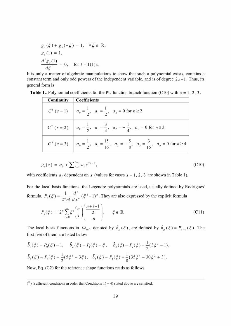
39

( ) ( ) 1, ,

(1) 1,

(1)0, for 1(1) .

s s

s

s

g g

g

d gs

d

ℓ

ℓ

ℝ

ℓ

It is only a matter of algebraic manipulations to show that such a polynomial exists, contains a

constant term and only odd powers of the independent variable, and is of degree 2 1s . Thus, its

general form is

Table 1.: Polynomial coefficients for the PU function branch function (C10) with 1, 2 , 3s .

Continuity Coefficients

1 ( 1)C s 0 1

1 1, , 0 for 2

2 2n

a a a n

2 ( 2 )C s 0 1 2

1 3 1, , , 0 for 3

2 4 4n

a a a a n

3 ( 3)C s 0 1 2 3

1 15 5 3, , , , 0 for 4

2 16 8 16n

a a a a a n

2 1

0 1( )

i s i

s iig z a a z

, (C10)

with coefficients ia dependent on s (values for cases 1, 2 , 3s are shown in Table 1).

For the local basis functions, the Legendre polynomials are used, usually defined by Rodrigues'

formula, 21( ) ( 1)

2 !

nn

n n n

dP

n d x . They are also expressed by the explicit formula

0

1

( ) 2 ,2n

n i

n

i

n in

Pi

n

ℝ . (C11)

The local basis functions in ref , denoted by ( )b ɶ , are defined by 1

( ) ( )b P ɶ . The

first five of them are listed below

2

1 0 2 1 3 2

3 4 2

4 3 5 4

1( ) ( ) 1, ( ) ( ) , ( ) ( ) (3 1) ,

2

1 1( ) ( ) (5 3 ) , ( ) ( ) (35 30 3).

2 8

b P b P b P

b P b P

ɶ ɶ ɶ

ɶ ɶ

Now, Eq. (C2) for the reference shape functions reads as follows

(12) Sufficient conditions in order that Conditions 1) – 4) stated above are satisfied.

40

( )( ) ( ) ( )su b ɶɶɶ . (C12)

Figure 2 shows both the local basis functions and the corresponding shape functions (in the refer-

ence domain ref ) for smoothness of order 2s . Note that ( )

1 ( ) ( )s

u ɶɶ .

Now, by using the affine transformation (C6), (C7), we are able to pass to the physical domain,

obtaining the PU functions ( )

( )s

k x , the local basis functions ( )k

b x , and the shape functions

( )ku x , for any subdomain k :

( ) ( )( ) ( ( ) )

s s

k kx x ɶ , ( ) ( ( ) )k

kb x b x ɶ (C13a,b)

( )( ) ( ) ( ) ( ( ) )

k s k

k ku x x b x u x ɶ . (C13c)

Figure 2. Legendre polynomial local basis functions ( )b ɶ (left panel) and corresponding shape

functions (2) ( ) ( )b ɶɶ (right panel), for different values of .

(c) PUFEM discretization and numerical solution of pdf evolution equations

Since the response pdf evolution equations, presented in Sec. 2 and 3 of the main paper, can at-

tain a variety of forms, the following generic form is adapted for developing the numerical

scheme

2

2

( , ) [ ; , ] ( , )( , ) ( , )

f x t f x t f x tq x t f x t

t x x

B

, (C14)

where now the unknown pdf is denoted by ( , )f x t instead of ( ) ( )X tf x . In Eq. (C14) ( , )q x t is

the drift coefficient, and [ ; , ]f x tB is the diffusion coefficient. Recall that the diffusion coeffi-

cient in VADA genFPK equations (41) depends on the unknown pdf ( , )f x t , rendering Eq.

41

(C14) nonlinear and nonlocal.(13) Nevertheless, in this subsection, the simple notation ( , )B x t

will be used for the diffusion coefficient, with notation [ ; , ]Xf x tB being employed in the next

subsection, where the treatment of nonlinearity/nonlocality will be explained.

Eq. (C14) is supplemented by the following conditions:

0 0( , ) ( ) knownf x t f x , (initial condition) (C15a)

( , ) 0 , ,f x t x ℝ (positivity condition) (C15b)

( , )f x t decays sufficiently fast as | |x . (14) (decay condition) (C15c)

In addition, the unknown function ( , )f x t should satisfy the condition

( , ) 1f x t d x

(C16)

since it is a probability density function. Note that this condition is automatically satisfied, since

the initial value 0 ( )f x is a pdf, and the integral (C16) is an invariant of Eq. (C14), as shown in

Appendix B(a) of this paper.

A weak form of Eq. (C14) is obtained by projecting both members on the elements ( )jv x of a

test function space, Test ( )V ℝ :

( ) ( )

( , ) ( ) ( , ) ( , ) ( )

j j

j j

S v S v

f x t v x d x q x t f x t v x d xt x

2

2

( )

( , ) ( , )( )

j

j

S v

B x t f x tv x d x

x

, (C17)

where ( ) supp ( ( ) )j j

S v v i . Integration by parts on both terms in the right-hand-side of Eq.

(C17) leads to the following equation, containing only first derivatives with respect to the un-

known function ( , )f x t :

( ) ( )

( ) ( )

( , ) ( , )( , ) ( ) ( ) ( , ) ( , ) ( )

( ) ( )( , ) ( , )( , ) ( , ) ( , ) .

j j

j j

j j j

S v S v

j j

S v S v

B x t f x tf x t v x d x v x q x t f x t v x

t x

v x v xB x t f x tq x t f x t d x B x t d x

x x x x

(C18)

To derive a discrete system of equations, the unknown solution ( , )f x t is approximated by us-

ing Eq. (C4):

( )

1 1

ˆ( , ) ( , ) ( ) ( ) ( ) ( )kK M

k k

m m

k m

f x t f x t w t u x w t u x

, (C19)

(13) This is not the case for the small correlation time genFPK Eq. (21) of the main paper, whose diffusion coeffi-

cient does not depend on the unknown response pdf.

(14) The appropriate decay rate at infinity needs for ensuring the existence of the integrals over the ℝ , which appear

in the weak form of Eq. (C10).

42

where ( ) ( )k

mw t w t are time-dependent weights, to be determined numerically, and the global

index ( , )m m k is defined by:

1

1 1

( , ) ( ) ( )k K

i i

m m k i i M

. (C20)

(Recall that ( )i denotes the number of basis functions in subdomain i

). Eq. (C20) can be

inverted, to derive ,k from m , by means of the formulae

1( ) max ( )

i j

ik k m j i m

:N ,

1 0

1 1( , ) ( ) , ( ) 0

i k i

i im k m i i

.

The integer 1

( )i K

iM i

counts the total number of shape functions used in the discretiza-

tion, and defines the global Degree of Freedom (DOF) of the scheme. To achieve better accura-

cy, the total DOF can be increased either by refining the cover { }k

(which corresponds to

h FE refinement), or by increasing the number ( )k of local basis functions in some (or all)

subdomains k

(which corresponds to p FE refinement), or both ( h p FE refinement).

In all applications presented herein, the test space Test ( )V ℝ is chosen to be the same as the ap-

proximation space P U ( )V (i.e. ( ) ( ) ,m mu x v x m ), i.e. Bubnov-Galerkin approach

(Hughes, 2000), leading to the following linear system:

( ) ( ) ( )t t tw wɺC A , (C21)

where:

,

( , )

( ) ( )

m j

M M

j m m j

S u u

c u x u x d x ℝC : (C22a)

,

( , )

( , )

( )( , )( ) : ( , ) ( )

( )( , ) ,

m j

m j

jM M

j m m

S u u

m j

S u u

u xB x tt t a q x t u x d x

x x

u u xB x t d x

x x

ℝA :

(C22b)

where ( , ) supp( ( ) ) supp( ( ) )m j m j

S u u u u i i . Note that the boundary terms of Eq. (C18) do

not appear in Eq. (C22b), since they are all zero because of the properties of PU functions.

Approximating the time derivative in Eq. (C21) by means of a Crank-Nicolson scheme and

grouping the terms with respect to their temporal argument, we obtain:

( ) ( ) ( ) ( )2 2

t tt t t t t t

w wC A A C (C23)

43

where t is the timestep. For each t , Eq. (C23) leads to an algebraic system of equations which

can be solved to obtain ( )t t w in terms of ( )tw . Initialization of the numerical scheme re-

quires knowledge of initial values of the weights 0 0

( )w t w , which are obtained by fitting the

PU representation 0

ˆ ( , )f x t to the known initial data 0

( )f x :

0 wC f (C24)

where:

0

( )

: ( ) ( )

j

M

j j

S u

f f x u x d x ℝf . (C25)

Numerical solution of the linear systems (C23), (C24) is performed via the SciPy (Jones et al.,

2001) interface to LAPACK’s (Anderson et al., 1999) routine GESV. For solving the problem

A X B , GESV performs an LU-decomposition with partial pivoting and row interchanges to

matrix A , namely A P LU , where P is a permutation matrix, L is unit lower triangular, and

U is upper triangular; the factored form of matrix A is used to solve the original system.

(d) Validation of the proposed scheme for the linear case

Having described the numerical scheme for the solution of genFPK equations, we shall now pre-

sent a first application to the simplest case that corresponds to the linear RDE under additive col-

oured noise excitation:

1( ; ) ( ; ) ( ; )X t X t t ɺ , 0 0( ; ) ( )X t X . (C28a,b)

As it is derived in Section 2(b) of the main paper, the response pdf of RDE (C28) satisfies exactly

the following genFPK equation (Eq. (18) of the main paper)

2

( ) ( )eff

1 ( ) ( ) 2

( ) ( )( ) ( ) ( )

X t X t

X t

f x f xx m t f x D t

t x x

i, (C29)

with effective noise intensity

0

0

0

1 1

(

( ) ( )eff 2

( ) ( )) ( )( ) ( , )

tt s

X

t t

t

D t e e C t s dsC t

i i i. (C30)

As proved previously in Appendix B, exact genFPK (C29) has the Gaussian pdf

2

( )

( ) 22( )( )

1 1( ) exp

2 ( )2 ( )

( )X t

XX

Xx

t

mx

tf

t

i

ii

(C31)

as its unique solution, with ( )

( )X

m ti

, 2

( ) ( )X ti

being the solutions to the linear ODEs (B12) and

(B13) respectively, which can be easily expressed in closed form as

1 0 1

0

0

( ) ( )

( ) ( )( ) ( )

tt t t

X

t

Xm t m e m e d

i i, (C32)

and

44

1 0 1

0

0 0

( ) ( )eff2 22

( ) 2 (( ))

tt t t

t

X X X e D e dt C i

. (C33)

Τhe numerical solution to genFPK Eq. (C29), obtained by using PUFEM with 200 degrees of

freedom (50 PU functions, each with 4 basis functions), is compared to the analytic solution

(C31) in Fig. 3 (left panels, a and c). Besides, in the right panels of Fig. 3, the approximate pdf

( )( )

X tf x , obtained by direct Monte Carlo (MC) simulations of RDE (C28), is compared to the

exact solution (C31). For the MC simulations, 45 10 realizations were solved and the pdf was

approximated using a kernel density estimator (Scott, 2015). As can be seen from Fig.3, numeri-

cal results indicate that both the PUFEM numerical scheme and the MC simulations are able to

accurately approximate the analytical solution. These results provide a first validation of the pro-

posed new pdf equation, as well as the implementation of the PUFEM numerical scheme for its

solution.

(e) Treatment of the nonlinear, nonlocal terms

As discussed above, a feature peculiar to VADA genFPK equations(15) is their nonlocality and

nonlinearity, coming from the dependence of the diffusion coefficient on the unknown pdf

through specific moments. The exact form of diffusion coefficient reads now as follows (see also

Eqs. (41) - (44) of the main paper):

0 0

( )eff eff

0 ( ) ( )

1 | |

; { ( )}[ ; , ] ( ) , ( ) ,

!

kM

t t

h m ht tm m

gx R tf x t D R t D R t

i

i ii i

α

α

φ

αB ,

(C34)

where ( ) ( ) ( ; )R s X s

i E for any function ( )x . As can be seen in Eq. (C34),

[ ; , ]f x tB depends on the current-time values of moments ( )

( )kgR t i , 1, ,k M … , as well as

on the whole time history(16) of moment ( ) ( )hR i i , via coefficients eff

mD :

0

0

0

eff

( ) ( ) ) 0([ ( ) , ] exp (( ) () )

tt m

m h ht

t

XD R t R u Cu t ttd

ii ii

0

2

( ) ( ) ( )exp ( ) ( , ) ( )

t t

m

h

t s

R u du C t s t s ds

i i i

. (C35)

(Eq. (C35) is obtained from Eq. (42) in conjunction with Eq. (39) of the main paper). Thus, in

each time step, we have to calculate the instantaneous values of the moments ( ) ( )hR t i ,

( )( )

kgR t i , 1, ,k M … (generically denoted by ( )R t ), and the integral ( )

( )t

hs

R u du i, which

is done by means of a prediction-correction iterative scheme as follows:

(15) In the case of nonlinear RDEs.

(16

) From initial time 0t to current time t .

45

Figure 3. Evolution of response pdf for the linear RDE (C28): 1 0.8 , 0.2 , under non-

zero mean Ornstein-Uhlenbeck excitation ( ( )0.2m

i , 1D , 1 ) and Gaussian initial data

0( 0.7Xm ,

00.15X ). Analytical solutions (round markers in panels (a) and (b)) are com-

pared to the PUFEM solution (panel (a)) and MC simulation approximation (panel (b)); errors of

PUFEM and MC against the analytical solution are shown in panels (c) and (d), respectively.

Initial time step 1i :

Calculate 0

( )R t from the given initial pdf

Set 1 0( ) ( )R t R t

(*) Set 1

( ) ( )R u du R t t , where t is the time step

Solve genFPK Eq. (C14) using PUFEM to find pdf 1

( , )f x t

Update 1

( )R t to a new value upd 1

( )R t , by using 1

( , )f x t

Check convergence condition 1 upd 1 tol( ) ( )R t R t , for a given error

tol

If convergence condition is not satisfied

Set 1 upd 1

( ) ( )R t R t and return to line (*)

Time marching 2, 3, ,i I … :

Calculate ( )i

R t via linear extrapolation of 1

( )i

R t and 2

( )i

R t

(&) Calculate ( )R u du using the previous and the current values ( )k

R t , 0 (1)k i

Solve genFPK Eq. (C14) using PUFEM to find pdf ( , )i

f x t

Update ( )i

R t to a new value upd

( )i

R t , by using ( , )i

f x t

46

Check convergence condition upd tol( ) ( )i iR t R t , for a given error tol

If convergence condition is not satisfied

Set upd

( ) ( )i i

R t R t and return to line (&)

Note that, in every time step, the iterative scheme typically converges within only a few (1-2) it-

erations.

47

Appendix D. Numerical Investigation of the range of validity of VADA genFPK equations

As in Section 4 of the main paper, we will consider here the dimensionless cubic RDE(17)

3( ; ) ( ; ) ( ; ) ( ; )X t X t X t t ɺ , 0 0( ; ) ( )X t X , (D1a,b)

under additive, zero-mean Ornstein-Uhlenbeck excitation ( ; )t with autocorrelation

( ) ( )

2 | |( , ) exp

D t sC t s

i i , (D2)

where D and are the dimensionless noise intensity and correlation time respectively. The pro-cedure and justification for formulating dimensionless RDE (D1a,b) and dimensionless excitation

autocorrelation (D2) can be found in Section 4 of the main paper.

By also considering that excitation ( ; )t is uncorrelated to initial value 0

( )X , the parame-

ters governing the behaviour of RDE (D1a,b) solution are only the dimensionless D and (18).

In Figures 4a,b below, we show, for various values of D and , the stationary response pdfs of

RDE (D1a,b) as calculated by solving the genFPK equations based on:

0th-order VADA (Hänggi’s ansatz), Eq. (41) of the main paper with 0M = (HAN),

2nd-order VADA, Eq. (41) of the main paper with 2M = (VADA-II) and

4th-order VADA, Eq. (41) of the main paper with 4M = (VADA-IV).

In the same Figures, the said stationary pdfs are compared with results obtained by Monte Carlo

(MC) simulations, in order to determine the range of parameter values in which HAN, VADA-II

and IV provide an accurate approximation.

For the MC simulations, the end of the transient state, st

t , is estimated by monitoring the station-

arity (time invariance) of the first two moments of the response. From this time instant stt for-

ward, we keep all simulation samples, with time step equal to the double of correlation time of excitation. This choice of time step ensures that we obtain uncorrelated samples. On the other

hand, HAN, VADA-II and VADA-IV stationary pdfs are obtained by solving the respective time-dependent genFPK equations from the initial time up to their stationary regime. The end of the

transient state of genFPK equations is taken equal to st

t of MC simulations; then we check that

their solutions remain unchanged for time equal to st

2 t , to ensure that they are indeed stationary.

By observing Figs. 4a,b, we come up with the following three remarks:

Remark D1: On the range of validity of Hänggi’s ansatz. For 0.2D and 1.0 (Fig. 4a),

HAN stationary pdfs are good approximations for 0.1 and 1.0 , while for larger noise intensi-

ty ( 2.0D in Fig. 4b), the good performance of HAN method is restricted to the small correla-

tion time regime ( 0.1 ). For even larger noise intensities ( 5.0D in Fig. 4b), HAN fails

(17

) Expressed here without tilde over the dimensionless quantities. (18) A more detailed investigation would also include as parameters the (non-zero in general) mean values of excita-

tion and initial value, as well as their cross-correlation.

48

even for 0.1 . In general, HAN method fails to capture the phenomenon of higher and nar-

rower pdf peaks as the parameter D increases, resulting thus in pdfs that are more diffusive

than the ones obtained by MC simulations. Roughly speaking, HAN becomes unreliable when

D becomes larger than 1.

Figure 4a. Stationary response pdf for RDE (D1a,b) excited by a zero-mean OU process with

0.2D (upper panel) and 1D (lower panel) and for 0.1,1.0 , 5.0 = . Results from HAN,

VADA-II and IV genFPK equations are presented along with MC simulations.

Remark D2: On the range of validity of VADA-II and IV methods. In Figs. 4a,b, we observe that the stationary pdfs obtained by solving VADA-II and IV genFPK equations are in good

49

agreement with pdfs obtained by MC simulations, even in cases where both D and attain large

values. Note that, even for 5.0D and 5.0 , VADA-II and IV continue to give acceptable

approximations of the stationary pdf. A general trend is that, as D and increase, VADA pdfs begin to fail at predicting the exact values and abscissae of the response pdf peaks. Roughly

speaking, the range of validity of VADAs method seems to be limited by the condition

25D < , providing a substantial improvement in comparison to HAN which is limited by the

condition 1D < .

Figure 4b. Stationary response pdf for RDE (D1a,b) excited by a zero-mean OU process with

2D (upper panel) and 5D (lower panel) and for 0.1,1.0 , 5.0 = . Results from HAN,

VADA-II and IV genFPK equations are presented along with MC simulations.

50

Remark D3: On the prediction of peak value drift. In Figs. 4a,b, we observe that, for large

values of D and , the pdfs obtained by MC simulations exhibit peak values at abscissae larger

than 1 in absolute value. This peak value drift, which has been documented before, see e.g.

(Hänggi and Jung, 1995) p. 294, is predicted quite accurately by VADAs in the regime of

( , ) [0, 5.0 ] [0, 5.0 ]D , with VADA-IV being consistently more accurate than VADA-II.

Note that this phenomenon is not captured at all by HAN, which predicts pdfs with peaks fixed at

1 .

References

Anderson, E. et al. (1999) LAPACK Users’ Guide. 3rd edn. SIAM.

Athanassoulis, G. A., Tsantili, I. C. and Kapelonis, Z. G. (2015) ‘Beyond the Markovian assumption: response-

excitation probabilistic solution to random nonlinear differential equations in the long time’, Proc.R.Soc.A, 471:(20150501).

Cetto, A. M., de la Peña, L. and Velasco R. M. (1984) ‘Generalized Fokker-Planck Equations for Coloured,

Multiplicative, Gaussian Noise’, Revista Mexicana de Física, 31(1), pp. 83–101. Fox, R. F. (1986) ‘Functional-calculus approach to stochastic differential equations’, Physical Review A, 33(1), pp.

467–476.

Gel’fand, I. M. and Vilenkin, N. Y. (1964) Generalized Functions vol. 4. Academic Press.

Hänggi, P. (1978) ‘Correlation functions and Masterequations of generalized (non-Markovian) Langevin equations’, Zeitschrift fur Physik B, 31, pp. 407–416. Hänggi, P. and Jung, P. (1995) ‘Colored Noise in Dynamical Systems’, Advances in Chemical Physics, 89, pp. 239–

326.

Hughes, T. J. R. (2000) The Finite Element Method: Linear Static and Dynamic Finite Element Analysis. Dover Publications.

Jones, E. et al. (2001) ‘SciPy: Open Source Scientific Tools for Python’. Available at: http://www.scipy.org/.

van Kampen, N. G. (2007) Stochastic Processes in Physics and Chemistry. 3rd edn. North Holland. Klyatskin, V. I. (2005) Stochastic Equations through the eye of the Physicist. Elsevier.

Kumar, M. et al. (2009) ‘The partition of unity finite element approach with hp-refinement for the stationary

Fokker–Planck equation’, Journal of Sound and Vibration, 327(1–2), pp. 144–162.

Kumar, M., Chakravorty, S. and Junkins, J. L. (2010) ‘A semianalytic meshless approach to the transient Fokker-Planck equation’, Probabilistic Engineering Mechanics, 25(3), pp. 323–331.

Lundgren, T. S. (1967) ‘Distribution functions in the statistical theory of turbulence’, The Physics of Fluids, 10(5), pp. 969–975. Melenk, J. M. and Babuska, I. (1996) ‘The partition of unity finite element method: Basic theory and applications’,

Computer Methods in Applied Mechanics and Engineering, 139(1–4), pp. 289–314.

Sancho, J. M. et al. (1982) ‘Analytical and numerical studies of multiplicative noise’, Physical Review A, 26(3), pp.

1589–1609. Sancho, J. M. and San Miguel, M. (1980) ‘External non-white noise and nonequilibrium phase transitions’,

Zeitschrift fur Physik B, 36, pp. 357–364.

Schwabl, F. (2006) Statistical Mechanics. 2nd edn. Springer-Verlag.

Scott, D. W. (2015) Multivariate Density Estimation. John Wiley & Sons, Inc. Sun, J. Q. (2006) Stochastic Dynamics and Control. Elsevier.

Venturi, D. et al. (2012) ‘A computable evolution equation for the joint response-excitation probability density function of stochastic dynamical systems’, Proc.R.Soc.A, 468, pp. 759–783.