A SYSTEM OF ODES FOR A PERTURBATION OF A MINIMAL MASS SOLITONmarzuola/MRS_final.pdf · A SYSTEM OF ODES FOR A PERTURBATION OF A MINIMAL MASS SOLITON 3 0:0 0:5 1:0 1:5 2:0 Soliton

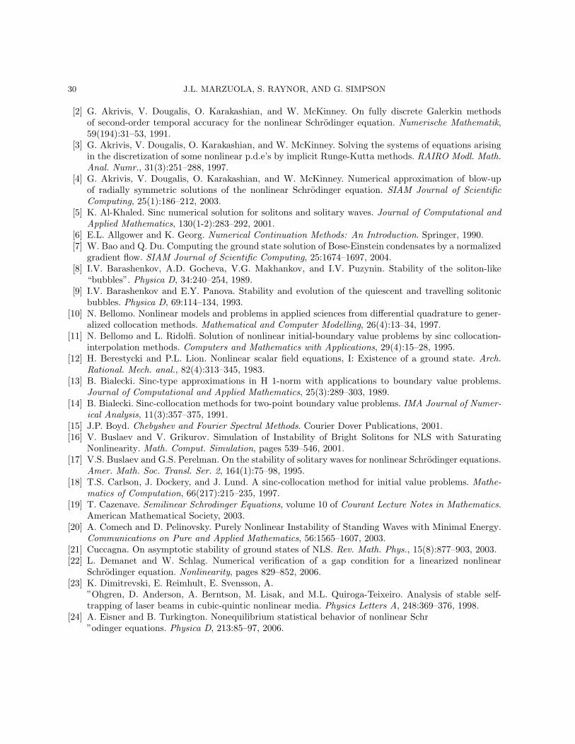
A SYSTEM OF ODES FOR A PERTURBATION OF A MINIMAL MASSSOLITON

JEREMY L. MARZUOLA, SARAH RAYNOR, AND GIDEON SIMPSON

Abstract. We study soliton solutions to the nonlinear Schrodinger equation (NLS) witha saturated nonlinearity. NLS with such a nonlinearity is known to possess a minimal masssoliton. We consider a small perturbation of a minimal mass soliton and identify a systemof ODEs extending the work of [20], which models the behavior of the perturbation forshort times. We then provide numerical evidence that under this system of ODEs there aretwo possible dynamical outcomes, in accord with the conclusions of [43]. Generically, initialdata which supports a soliton structure appears to oscillate, with oscillations centered ona stable soliton. For initial data which is expected to disperse, the finite dimensionaldynamics initially follow the unstable portion of the soliton curve.

1. Introduction

The nonlinear Schrodinger equation (NLS) in Rd × R+:

(1.1) iut + ∆u+ g(|u|2)u = 0, u(x, 0) = u0(x)

emerges as a leading order description of important physical systems in optics, many bodyquantum systems, hydrodynamics, and plasma physics. Moreover, it is a canonical equationdemonstrating the competition between nonlinearity and dispersion.

In many applications, the leading order approximation of the nonlinearity, g(s), is thepower nonlinearity g(s) = ±sσ. For example, g(s) = s, yields the focusing cubic NLSequation. Cubic NLS appears in many contexts, including many body quantum quantumsystems, when the Hartree equation is approximated with pairwise delta funciton interac-tions. It similarly appears in nonlinear optics if the higher order corrections to the nonlinearindex of refraction are neglected.

Such approximations may lead to non-physical predictions. In the case of the power-lawnonlinearity, if σd ≥ 2, initial data with mass (L2 norm) in excess of the ground state mayblow up in finite time [58]. However, experiments in the optical setting show that there isno “singularity” to speak of; the intensity of the solutions remains finite [34].

The model equation can be corrected to suppress singularity formation by replacingthe power nonlinearity with a saturated nonlinearity. Ideally, such a nonlinearity allowspotentially unstable behavior at low intensity but regularizes it at high intensity. Oneexample of such a nonlinearity is the cubic-quintic, where g(s) = s − γs2. The cubic-quintic NLS (CQNLS) equation appears as a correction to the many body system that

1

2 J.L. MARZUOLA, S. RAYNOR, AND G. SIMPSON

includes (repulsive) three body delta function interactions [8, 9]. CQNLS also appears inmodels of super fluids, [33], and in nonlinear optics, [23,45,62].

Another saturated nonlinearity appearing optics literature is g(s) = s/(1 + s), [59]. Thisnonlinearity was used in [24] to study turbulence for a one dimensional, non-integrableequation without singularity formation. In laser plasma interactions, g(s) = 1 − e−s isused, [31]. In all cases, the Taylor expansion of the nonlinearity leads to CQNLS at secondorder.

In this work we consider saturated nonlinearities of the form

(1.2) g(s) = sq2

sp−q2

1 + sp−q2

,

where 2 + 4d−2

> p > 2 + 4d> 4

d> q > 0 for d ≥ 3 and ∞ > p > 2 + 4

d> 4

d> q > 0 for

d < 3. For |u| large, (1.1) behaves as though it were L2 subcritical while for |u| small, itbehaves as though it were L2 supercritical. Note that this choice of saturated nonlinearityis focusing for all values of |u|. For our purposes, p must be chosen substantially largerthan the L2 critical exponent, 4

d, in order to allow sufficient regularity when linearizing the

equation. For our numerical analysis, we work in one spatial dimension with the specificnonlinearity

(1.3) g(s) =s3

1 + s2.

A soliton solution of (1.1) is a function u(t, x) of the form

(1.4) u(t, x) = eiωtφω(x),

where ω > 0 and φω(x) is a positive, spherically symmetric, exponentially decaying solutionof the equation:

(1.5) ∆φω − ωφω + g(φ2ω)φω = 0.

For our particular nonlinearity, for any ω > 0 there is a unique solitary wave solution φω(x)to (1.5), see [12] and [41].

For large ω the solitons are stable, while for small ω they are unstable. A precise stabilitycriterion identifying stable and unstable regions is provided in [29] and [51], generalizingearlier work on stability in [60], [61]. This amounts to examining the relation ω 7→ ‖φω‖2

L2 ,defining a soliton curve. Where it is increasing as a function of ω, the solitons are stable;where this function is decreasing the solitons are unstable. In Figure 1 we plot this curvefor several common choices of g(s).

As can be seen numerically in Figure 1, our saturated nonlinearity spawns a soliton ofminimal mass. Certain asymptotic methods can be used to describe the nature of the curve–multiscale methods can provide the asymptotics as ω → 0, while variational methods cangive the asymptotics as ω → ∞. However, in this work we forego an analytic descriptionof the soliton curve and focus on the minimal mass soliton shown to exist in the numerical

A SYSTEM OF ODES FOR A PERTURBATION OF A MINIMAL MASS SOLITON 3

0.0 0.5 1.0 1.5 2.0Soliton Parameter, ω

0

2

4

6

8

10

Mas

s,Qω

Saturating NLSCubic NLSQuintic NLSSeventh Order NLS

Figure 1. Plots of the soliton curves (φ(ω) with respect to ω) for a sub-critical nonlinearity, critical nonlinearity, supercritical nonlinearity, and thesaturated nonlinearity (1.3). The curves for the monomial nonlinearities arefound analytically, while the curves for the saturated nonlinearities are foundnumerically using the method discussed in Section 4.1. All are in d = 1. Hereω ≥ .001, as the supercritical and saturated cases diverge as ω → 0.

plot. The minimal mass solution is a distinguished case amongst the already special familyof soliton solutions. Though solitons to the left and right of this minimum can readily beclassified as stable or unstable, the theory fails at extrema [60,61]. This motivates a carefulexamination of the dynamics of the minimal mass soliton under perturbation.

In [20], Comech and Pelinovsky demonstrated that the minimal mass soliton possesses afundamentally nonlinear instability. They accomplished this by finding a small perturba-tion that forces the solution a fixed distance away from the minimal mass soliton in finitetime. Their technique reduces the problem to studying an ODE modeling the perturbationfor short times. They show that the 0 solution to the ODE is unstable by appropriatechoice of initial data.

The purpose of this work is to numerically explore the following conjecture:

Conjecture 1.1. Though the minimal mass soliton is unstable on short time scales, weconjecture that, on longer time scales, any solutions which is initially a small perturbationof the minimal mass soliton will either disperse or eventually relax towards a nearby stablesoliton.


This conjecture is part of the more general conjecture that any solution which does notdisperse as t→∞ must eventually converge to a finite sum of stable solitons. Although theequation has a branch of unstable solitons, physically, it is expected that general solutionsto (1.1) will resolve into stable solitons plus a dispersive component. This is referred toas the “soliton resolution” conjecture, a notoriously difficult problem to formulate. Fornonlinearities with a specific two power structure, dynamics of this type were observed byPelinovsky, Afanasjev, and Kivshar, who modelled the behavior of solutions near a minimalmass soliton by a second order ODE via adiabatic expansion in ω [43]. This conjecturehas also been explored numerically by Buslaev and Grikurov for two power nonlinearitiesin [16], where they found that a solution which is initially a perturbation of an unstablesoliton tends to approach and then oscillate around a stable soliton.

By contrast, our method uses the full dynamical system of modulation parameters to finda 4-dimensional system of ODEs which is structured to allow for eventual recoupling to thecontinuous spectrum. Following [20], we begin with the ansatz that our solution is a smallperturbation of the minimal mass soliton. We then break the perturbation into discreteand continuous spectral components relative to the linearization of the Schrodinger operatorabout the soliton. The discrete portion yields a four dimensional system of nonlinear ODEs.In this work, we neglect the continuous spectrum, although it may be included in a futurework. We further simplify the system expanding the equations in powers of the dependentvariables and dropping cubic and higher terms.

An obstacle in studying these ODEs is that the signs and magnitudes of the coefficientsare not self-evident, necessitating numerical methods. We compute these values, whichare intimately related to the minimal mass soliton, using the sinc spectral method. Theuse of the sinc function for numerically solving differential equations dates to Stenger [54].It has been successfully used in a wide variety of linear and nonlinear, time dependentand independent, differential equations [5, 11, 14, 18, 25, 38, 46, 57]. In this work, we firstnumerically solve (1.5) for the soliton as a nonlinear collocation problem. We then use thisinformation to compute the generalized kernel of the operator after linearization about thesoliton.

With these coefficients in hand, we numerically integrate the ODE system, plotting theresults. We find that there are two different types of behavior for the finite dimensionalsystem, depending on the initial data. If the initial data represents a solution which ournonlinear PDE solver indicates can support a soliton, then we find that the solution isoscillatory. It is initially attracted to the stable side of the curve, and, over intermediatetime scales, oscillates around a stable soliton close to the minimal mass soliton. If weinitialize with the unstable conditions found in [20], the ODEs initially move in the unstabledirection but quickly reverse, before commencing oscillation. On the other hand, if we beginwith initial conditions which are expected to disperse as t → ∞, the finite dimensionaldynamics push the solution along the unstable soliton curve towards the value ω = 0rather quickly. This solution agrees with the numerically computed solution of the primitive


equation (1.1) with corresponding initial data for as long as the mass conservation of thesolution allows, after which our model continues to follow the unstable soliton curve butthe actual solution disperses. In [43], the authors observed similar dynamics, with bothoscillatory and dispersive regimes.

These ODEs are an approximation valid on a short time interval. This study is thebeginning of an analysis to show that perturbations of the minimal mass soliton are at-tracted to the stable side of the soliton curve. In a forthcoming work we hope to showhow the continuous-spectrum part of the perturbation interacts with the discrete-spectrumperturbation. Based on the work of Soffer and Weinstein, [53] we expect coupling to thecontinuous spectrum to cause radiation damping, which will ultimately cause the solutionto have damped oscillations and select a soliton on the stable side of the curve.

This paper is organized as follows. In section 2, we introduce preliminaries and necessarydefinitions. In section 3, we derive the system of ODEs. In section 4, we explain ournumerical methods for finding the coefficients of the ODEs. In section 5, we show thenumerical solutions of the ODEs and explain our results. Finally, in section 6 we presentour conclusions and plans for future work. An appendix contains details of our numericalmethod for computation of the soliton and related coefficients.

Acknowledgments This project began out of a conversation with Catherine Sulemand JLM. JLM was partially funded by an NSF Postdoc at Columbia University and aHausdorff Center Postdoc at the University of Bonn. In addition, JLM would like to thankthe University of North Carolina, Chapel Hill for graciously hosting him during part of thiswork. SR would like to thank the University of Chicago for their hospitality while someof this work was completed. GS was funded in part by NSERC. In addition, the authorswish to thank Dmitry Pelinovsky, Mary Pugh, Catherine Sulem and Michael Weinstein forhelpful comments and suggestions.

2. Definitions and Setup

Equation (1.1) is globally well-posed in H1, the usual Sobolev space, with norm

‖u‖2H1 = ‖u‖2

L2 + ‖∇u‖2L2 .

The global well-posedness for initial data in H1 follows from the standard well-posednesstheory for semilinear Schrodinger equations. Additionally, we assume that u0 is sphericallysymmetric (which means even in one dimension), implying u(x, t) = u(|x|, t) for all t > 0.Proofs can be found in numerous references including [19] and [58].

For data u0 ∈ H1, there are several conserved quantities. Particularly important invari-ants are:

Conservation of Mass (or Charge):

Q(u) =1

2

∫Rd

|u|2dx =1

2

∫Rd

|u0|2dx.


Conservation of Energy:

E(u) =

∫Rd

|∇u|2dx−∫

Rd

G(|u|2)dx =

∫Rd

|∇u0|2dx−∫

Rd

G(|u0|2)dx,

where

G(t) =

∫ t

0

g(s)ds.

Detailed proofs of these conservation laws can be easily arrived at by using energy esti-mates or Noether’s Theorem, which relates conservation laws to symmetries of an equation.See [58] for details.

With this type of nonlinearity, it is known that soliton solutions to NLS exist and areunique. Existence of solitary waves for nonlinearities of the type (1.2) is proved by in [12]in R1 using ODE techniques and in higher dimensions by minimizing the functional

T (u) =

∫|∇u|2dx

with respect to the functional

V (u) =

∫[G(|u|2)− ω

2|u|2]dx.

Then, using a minimizing sequence and Schwarz symmetrization, one infers the existenceof the nonnegative, spherically symmetric, decreasing soliton solution. Once we know thatminimizers are radially symmetric, uniqueness can be established via a shooting method,showing that the desired soliton occurs at only one initial value, [41].

Of great importance is the fact that Qω := Q(φω) and Eω := E(φω) are differentiablewith respect to ω. This can be determined from the works of Shatah, namely [49], [50].Differentiating (1.5), Q and E all with respect to ω, we have the relation

∂ωEω = −ω∂ωQω.

Numerical computations show that if we plot Qω with respect to ω for the saturatednonlinearity, the soliton curve goes to ∞ as ω goes to 0 or ∞ and has a global minimumat some ω = ω∗ > 0; see Figure 1.

We are interested in the stability of these explicit solutions under perturbations of theinitial data. Recall the following notions of stability:

Definition 2.1. The soliton is said to be orbitally stable if, ∀ε > 0, ∃δ > 0 such that,for any initial data u0 such that ‖u0 − φω‖H1 < δ, for any t < 0, there is some θ ∈ R suchthat ‖u(x, t)− eiθφω(x)‖H1 < ε.

Definition 2.2. The soliton is said to be asymptotically stable, if, ∃δ > 0 such that if

‖u0−φω‖H1 < δ, then ∃ω, θ > 0 and ψ0 ∈ H1 such that ‖u(x, t)−eiωt+θφω(x)−eit∆ψ0‖H1 →0 as t→∞.


Remark 2.1. Orbital stability suggests that a solution to (1.1) initially near the solitonwill remain near the soliton in the H1 norm. However, asymptotic stability states that thesystem actually selects a specific soliton to converge to as time goes to ∞. Note, technicallya system can undergo a very large change in ω and still be “asymptotically stable” providedit converges to a soliton for large time. However, asymptotic stability is usually provedusing perturbation theory, which would suggest that in Definition 2.2, there would exist anε > 0 depending on δ such that

|ω − ω| < ε.

Variational techniques developed in [60], [61] and generalized to an abstract setting in [29]and [51] tell us that when δ(ω) = Eω + ωQω is convex, or δ′′(ω) > 0, we are guaranteedstability under small perturbations, while for δ′′(ω) < 0 we are guaranteed that the solitonis unstable under small perturbations. For brief reference on this subject, see Chapter4 of [58]. For nonlinearities that are twice differentiable at the origin and of monomialtype at infinity (which would include our saturated nonlinearities), asymptotic stabilityhas been studied for a finite collection of strongly orbitally stable solitons by Buslaev andPerelman [17], Cuccagna [21], and Rodnianski, Soffer and Schlag [47].

At a minimum of Qω, soliton instability is more subtle, because it is due solely to nonlin-ear effects. See [20], where this purely nonlinear instability is proved to occur by reducingthe behavior of the discrete part of the spectrum to an ODE that is unstable for certaininitial conditions.

2.1. Linearization about a Soliton. Throughout this section, we use vector notation,~·,to represent complex functions. Any function written without vector notation is assumed

to be real. For example, the complex valued scalar function u+ iv will be written

(uv

). In

this notation, multiplication by i is represented by the matrix J =

(0 −11 0

). We denote

by ~φω the complex vector

(φω0

), where φω is the real profile of the soliton with parameter

ω. For simplicity, we suppress the ω subscript, writing φ in place of φω.

For later reference, we now explicitly characterize the linearization of NLS about a solitonsolution. First consider the linear evolution of the perturbation of a soliton via the ansatz:

(2.1) ~u = eJωt(~φω(x) + ~ρ(x, t))

with ~ρ =

(ρReρIm

). For the purposes of finding the linearized Hamiltonian at φω we do not

need to allow the parameters θ and ω to modulate, but when we develop our full systemof equations in Section 3 parameter modulation will be taken into account. Inserting (2.1)


as an ansatz into (1.1) we know that since φ is a soliton solution we have

(2.2) J(~ρ)t + ∆(~ρ)− ω~ρ = −g(φ2)~ρ− 2g′(φ2)φ2

(ρRe0

)+O(|~ρ|2).

(This calculation is explained in more detailed at the start of Section 3.) Here we haveused the following calculation of the nonlinear terms of the perturbation equation:

(g(|φ+ ρ|2)(φ+ ρ)− g(|φ|2)φ) = (g(φ2 + 2φρRe + ρ2Re + ρ2

Im)(φ+ ρRe + iρIm)− g(φ2)φ)

= g′(φ2)(ρ2Re + 2φρRe + ρ2

Im)(φ+ ρRe + iρIm)

+1

2g′′(φ2)(ρ2

Re + 2φρRe + ρ2Im)2(φ+ ρRe + iρIm) + h.o.t.s.(2.3)

The linear terms will be absorbed into the linearized operator JHω, while the quadraticterms are handled explicitly; the O(ρ2) terms in the expansion of the equation around φωwill be denoted by N(ω, ρ) in the sequel. In this work, after expansion in powers of ρ, wedrop all terms of order greater than two.

We are interested in linearizing this equation:

(2.4) ∂t

(ρReρIm

)= JH

(ρReρIm

)+ h.o.t.,

where

H =

(0 L−−L+ 0

),(2.5)

L− = −∆ + ω − g(φω),(2.6)

L+ = −∆ + ω − g(φω)− 2g′(φ2ω)φ2

ω.(2.7)

Definition 2.3. A Hamiltonian, H is called admissible if the following hold:1) There are no embedded eigenvalues in the essential spectrum,2) The only real eigenvalue in [−ω, ω] is 0,3) The values ±ω are non-resonant .

Definition 2.4. Let (NLS) be taken with nonlinearity g. We call g admissible if thereexists a minimal mass soliton, φmin, for (NLS) and the Hamiltonian, H, resulting fromlinearization about φmin is admissible in terms of Definition 2.3.

The spectral properties assumed for the linearized Hamiltonian equation in order to provestability results are typically those from Definition 2.3, see [17, 22, 48, 47, 35, 28]. However,we note that this condition is a constraint used to control the dispersive estimates necessaryfor perturbative analysis in analytic results, though it is sometimes possible to numericallysolve this sort of problem even if Definition 2.3 does not hold; see, for example, [16].

In this work, we must simply assume that g is an admissible nonlinearity so that wemust only concern ourselves with known discrete spectrum functions without coupling to


endpoint resonances or embedded eigenvalues. However, this assumption is justified bythe observed dynamics. Great care must be taken in studying the spectral properties of alinearized operator; although admissibility is expected to hold generically, certain algebraicconditions on the soliton structure itself must factor into the analysis, often requiring carefulnumerical computations. See [22] as an introduction to such methods and the difficultiestherein. To this end, in the forthcoming work [40], two of the authors will look at analyticand computational methods for verifying these spectral conditions.

2.2. The Discrete Spectral Subspace. We approximate perturbations of the minimalmass soliton by projecting onto the discrete spectral subspace of the linearized operator.Notationally, we refer to Pd as the projection onto the finite dimensional discrete spectralsubspace Dω of H1 relative to H. Similarly, Pc represents projection onto the continuousspectral subspace for H. We now describe, in detail, the discrete spectral subspace at theminimal mass.

Let ω∗ be the value of the soliton parameter at which the minimal mass soliton occurs.It is proved in [20] (Lemma 3.8) that the discrete spectral subspace Dω of H at ω∗ hasreal dimension 4. This results from the extra orthogonality at minimal mass, which givesa dimension 4 generalized kernel given by the following chain of equalities

L−φω∗ = 0,

L+(−φ′ω∗) = φω∗ ,

L−α = −φ′ω∗ ,L+β = α.

The functions ~e1 =

(0φω

)and ~e2 =

(φ′ω0

)are in the generalized kernel of H at every ω.

Clearly, ~e1 is purely imaginary and ~e2 is real. In addition to ~e1 and ~e2, at ω∗ there are two

more linearly independent elements of Dω, the purely imaginary ~e3 =

(0α

)and the purely

real ~e4 =

(β0

).

Applying [20] (Lemma 3.9), ~e3 and ~e4 can be extended as continuous functions of ω insuch a way that ~e3(ω) is purely imaginary, ~e4(ω) is purely real. We write

~e3(ω) =

(0

α(ω)

)and

~e4(ω) =

(β(ω)

0

),


with α and β real-valued functions. The linearized operator, restricted to this subspace, is

(2.8) JH(ω)|Dω =

0 1 0 00 0 1 00 0 0 10 0 a(ω) 0

,

where a(ω) is a differentiable function that is equal to 0 at ω∗.

Before proceeding to the derivation of the ODEs, it is helpful to make a minor change

of basis. Our goal is that, in the new basis,{~e1, ~e2, ~e3, ~e4

},⟨~e1, ~e3

⟩= 0, which will make

it easier for us to compute the dual basis. Replace ~e3 by

~e3 = ~e3 −〈~e1, ~e3〉‖~e1‖2

~e1

=

[0α

].

To preserve the relationship ~e3 = JHω~e4, we need to replace ~e4 by

~e4 = ~e4 −〈~e1, ~e3〉‖~e1‖2

~e2

=

[β0

].

To preserve the relationship JHω~e3 = ~e2 + a(ω)~e4, we replace ~e2 by

~e2 =

(1 +〈~e1, ~e3〉‖~e1‖2

)~e2

=

[e2

0

].

To preserve JHω~e2 = ~e1, we get that ~e1 must be replaced by

~e1 =

(1 +〈~e1, ~e3〉‖~e1‖2

)~e1

=

[0e1

].

With these substitutions, the JHω matrix on Dω remains the same and we obtain the

relationship⟨~e3, ~e1

⟩= 0. From here on we will assume that we are working with this

modified basis and simply take ~ej := ~ej for j = 1, 2, 3, 4.

We will define ~ξi to be the dual basis to the revised ~ei within Dω. That is, the ~ξi are

defined by ~ξi ∈ Dω and

〈~ξi, ~ej〉 = δij.


If we make the change of basis described above, then we can compute the ~ξj as follows.Define D = ‖~e2‖2‖~e4‖2 − 〈~e2, ~e4〉2. Then:

~ξ1 =1

‖~e1‖2~e1,

~ξ2 =‖~e4‖2

D~e2 −

〈~e2, ~e4〉D

~e4,

~ξ3 =1

‖~e3‖2~e3,

~ξ4 = −〈~e2, ~e4〉D

~e2 +‖~e2‖2

D~e4.

As with the ~ej’s,

~ξj =

[0ξj

]for j = 1, 3 and

~ξj =

[ξj0

]for j = 2, 4 to distinguish between vectors and their scalar components.

3. Derivation of the ODEs

To derive the ODEs we start with a small spherically symmetric perturbation of theminimal mass soliton, then project onto the discrete spectral subspace. Here, we closelyfollow [20].

We begin with the following ansatz, which allows theta and ω to modulate:

(3.1) ~u(t) = e(R t0 ω(t′)dt′+θ(t))J(~φω(t) + ~ρ(t)).

Here we are suppressing the dependence of u, φ, and ρ on |x| for notational simplicity.Recall, we have assumed u to be spherically symmetric, so no other modulation parametersoccur. Unlike in [20] we do not assume that the rotation variable θ(t) is identically zero, sowe need to include θ modulation in our full ansatz. Note that the derivation which followsapplies for all nonlinearities in any dimension; specialization is required only to get explicitnumerical results. This model includes the full dynamical system for spherically symmetricdata and is designed in such a way that coupling to the continuous spectral subspace couldeasily be reintroduced. The authors plan to analyze the effect of that coupling, which isexpected to be dissipative, in a future work.

Differentiating (3.1) with respect to t, we get

~ut = [(ω + θ)J(~φ+ ~ρ) + ω~φ′ + ~ρ]ei(R t0 ω(t′)dt′+θ(t)),


where for a time dependent function g(t) we represent differentiation with respect to t by∂tg = g and for an ω dependent function f(ω) we denote differentiation with respect tothe soliton parameter ω by ∂ωf = f ′. Plugging the above ansatz into equation (1.1) andcancelling the phase term yields

(3.2) − (ω + θ)(~φ+ ρ) + ωJ ~φ′ + J~ρ+ ∆~φ+ ∆~ρ+ g(|φ+ ρ|2)(~φ+ ~ρ) = 0.

Recall that since φ is a soliton solution, −ωφ+ ∆φ+ g(|φ|2)φ = 0, yielding

(3.3) − θ~φ− (ω + θ)(~ρ) + ωJ ~φ′ + J~ρ+ ∆~ρ+ g(|~φ+ ~ρ|2)(~φ+ ~ρ)− g(φ2)φ = 0.

We multiply by J , solve for ~ρ, and simplify. At the same time, we collect the ∆~ρ and

−ω~ρ terms with the linear portion of g(|~φ + ~ρ|2)(~φ + ~ρ) − g(φ2)~φ, which yields JHω asdefined in (2.5). The remaining terms of the nonlinearity are at least quadratic in ρ; recallthat the quadratic terms are described in (2.3) and denoted N(ω, ρ).

Defining ρj(t) as the coefficient of ~ej(t) in ρ, we have

~ρ =

[ρReρIm

]= ρ1~e1 + ρ2~e2 + ρ3~e3 + ρ4~e4 + ~ρc.

Then, the above calculations give us

(3.4) ~ρ = JHω~ρ− θ(

0φ

)− θJ~ρ− ω

(φ′

0

)+ ~N(ω, ~ρ).

Taking the inner product of (3.4) with each of the ~ξi as defined in Section 2.2, andapplying (2.8) yields the following system:

〈~ξ1, ~ρ〉 = ρ2 − θ − θ〈~ξ1, J~ρ〉+ 〈~ξ1, ~N〉,

〈~ξ2, ~ρ〉 = ρ3 − ω − θ〈~ξ2, J~ρ〉+ 〈~ξ2, ~N〉,

〈~ξ3, ~ρ〉 = ρ4 − θ〈~ξ3, J~ρ〉+ 〈~ξ3, ~N〉,(3.5)

〈~ξ4, ~ρ〉 = a(ω)ρ3 − θ〈~ξ4, J~ρ〉+ 〈~ξ4, ~N〉.

From this point forward in our approximation we drop the ~ρc component as a higher ordererror term. Using the product rule, we solve the left hand side for ρi and put the extraterms from the derivative of the operator that projects onto the discrete spectral subspaceonto the right hand side.

We have, as in [20], that

Pd~ρ =∑

~ej ρj + ω∑

~eiΓijρj − ωPdP ′d~ρ,

where we have implicitly defined

Γij = 〈ξi, e′j〉


and used that

Pdd

dtPc~ρ = −ωPdP ′d~ρ.

This gives

ρ1 + θ = ρ2 − θ〈~ξ1, J~ρ〉+ 〈~ξ1, ~N〉+ ω(〈~ξ1, P′d~ρ〉 −

∑Γ1jρj),

ρ2 + ω = ρ3 − θ〈~ξ2, J~ρ〉+ 〈~ξ2, ~N〉+ ω(〈~ξ2, P′d~ρ〉 −

∑Γ2jρj),

ρ3 = ρ4 − θ〈~ξ3, J~ρ〉+ 〈~ξ3, ~N〉+ ω(〈~ξ3, P′d~ρ〉 −

∑Γ3jρj),(3.6)

ρ4 = a(ω)ρ3 − θ〈~ξ4, J~ρ〉+ 〈~ξ4, ~N〉+ ω(〈~ξ4, P′d~ρ〉 −

∑Γ4jρj).

There is also coupling to the continuous spectrum through terms such as 〈~ξ1, J~ρ〉 which weomit. This can be included in the error term and is not analyzed in our finite dimensionalsystem.

To make the system well-determined, we must introduce two orthogonality conditions.The first is 〈ρ, e2〉 = 0, and the second is 〈ρ, e1〉 = 0. These represent the choice of ω(t) andθ(t) respectively that minimize the size of ρ, which yields ρ2 = ρ2 = 0, and ρ1 = ρ1 = 0,respectively.

The reduced system is then:

θ = −θ〈~ξ1, J~ρ〉+ 〈~ξ1, ~N〉+ ω(〈~ξ1, P′d~ρ〉 −

∑Γ1jρj),

ω = ρ3 − θ〈~ξ2, J~ρ〉+ 〈~ξ2, ~N〉+ ω(〈~ξ2, P′d~ρ〉 −

∑Γ2jρj),

ρ3 = ρ4 − θ〈~ξ3, J~ρ〉+ 〈~ξ3, ~N〉+ ω(〈~ξ3, P′d~ρ〉 −

∑Γ3jρj),(3.7)

ρ4 = a(ω)ρ3 − θ〈~ξ4, J~ρ〉+ 〈~ξ4, ~N〉+ ω(〈~ξ4, P′d~ρ〉 −

∑Γ4jρj).

In [20], the authors further reduce this system to prove there is an initial nonlinearinstability. (Note that they have a slightly different system because they have assumedthat θ ≡ 0.) We are interested in the dynamics on an intermediate time scale; thus, weretain quadratically nonlinear terms in our equations.

Our notation is as follows. First, we have

〈~ξ1, J~ρ〉 = 〈ξ1, ρ2φ′ + ρ4β〉

= ρ4〈ξ1, β〉,since ρ2 = 0. Denote

c14 = 〈ξ1(ω∗), β(ω∗)〉,which is the highest order term and the only one that will figure into our quadratic expan-sion. Notice that this is a real inner product of functions that normally do not appear inthe same component of the complex vectors, because of the J in the equation.


Similarly, we have

〈~ξ2, J~ρ〉 = 〈ξ2,−ρ1φ− ρ3α〉= −ρ3〈ξ2, α〉,

since ρ1 = 0. Denote

c23 = 〈ξ2(ω∗), α(ω∗)〉,which is again the highest order term.

Then we have

〈~ξ3, J~ρ〉 = 〈ξ3, ρ2φ′ + ρ4β〉

= ρ4〈ξ3, β〉,

since ρ2 = 0. Denote

c34 = 〈ξ3(ω∗), β(ω∗)〉.

Finally, we have

〈~ξ4, J~ρ〉 = 〈ξ4,−ρ1φ− ρ3α〉= −ρ3〈ξ4, α〉,

since ρ1 = 0. Denote by

c43 = 〈ξ4(ω∗), α(ω∗)〉.

We also write gij for the term Γij(ω) = 〈~ξi, ~e′j〉 at ω = ω∗.

Next, consider the terms 〈~ξj, P ′d~ρ〉. These terms are the ej components of P ′d~ρ. We have:

PdP′d~ρ = Pd

[4∑j=1

〈~ξ′j, ~ρ〉~ej +4∑j=1

〈~ξj, ~ρ〉~e′j

]

=4∑j=1

4∑k=3

〈~ξ′j, ~ek〉ρk~ej + ρ3Pd~e′3 + ρ4Pd~e

′4

=4∑j=1

4∑k=3

〈~ξ′j, ~ek〉ρk~ej + ρ3(Γ13~e1 + Γ33~e3) + ρ4(Γ24~e2 + Γ44~e4)

= 〈~ξ′1, ~e3〉ρ3~e1 + 〈~ξ′2, ~e4〉ρ4~e2 + 〈~ξ′3, ~e3〉ρ3~e3 + 〈~ξ′4, ~e4〉ρ4~e4

ρ3(Γ13~e1 + Γ33~e3) + ρ4(Γ24~e2 + Γ44~e4)

= (〈~ξ′1, ~e3〉+ Γ13)ρ3~e1 + (〈~ξ′2, ~e4〉+ Γ24)ρ4~e2

+ (〈~ξ′3, ~e3〉+ Γ33)ρ3~e3 + (〈~ξ′4, ~e4〉+ Γ44)ρ4~e4.


Therefore, the relevant nonzero terms are

〈~ξ1, P′d~ρ〉 = (〈~ξ′1, ~e3〉+ Γ13)ρ3,

〈~ξ2, P′d~ρ〉 = (〈~ξ′2, ~e4〉+ Γ24)ρ4.

We denote

p13 = 〈~ξ′1(ω∗), ~e3(ω∗)〉,

p33 = 〈~ξ′3(ω∗), ~e3(ω∗)〉,

and

p24 = 〈~ξ′2(ω∗), ~e4(ω∗)〉,

p44 = 〈~ξ′4(ω∗), ~e4(ω∗)〉.

Note that some cancellation will occur with the Γij terms that appear separately in thesystem of ODEs, leaving only these pij terms in the finally system.

Finally, the terms 〈~ξi, ~N(ω, ~ρ)〉 must be computed. We are only interested in the qua-dratic terms, which, according to (2.3) are:

(3.8) 3Jg′(φ2)φρ2Re + 2Jg′′(φ2)φ2ρ2

Re + Jg′(φ2)φρ2Im + 2g′(φ2)φρReρIm.

Recall that, since ρ1 and ρ2 are 0, the projection onto the discrete-spectrum of ρRe is justρ3~e3 and the projection onto the discrete-spectrum of ρIm is just ρ4~e4. We now have tocompute the lowest-order terms of

〈~ξ1, ~N(ω, ~ρ)〉.

The multiplier of ρ23 in 〈~ξ1, ~N(ω, ~ρ)〉 is

n133 = 〈ξ1, (3g′(φ2)φ+ 2g′′(φ2)φ2)e2

3〉.

Similarly, we define

n144 = 〈ξ1, g′(φ2)φe2

4〉,n234 = 〈ξ2,−2g′(φ2)φe3e4〉,n333 = 〈ξ3, (3g

′(φ2)φ+ 2g′′(φ2)φ2)e23〉,

n344 = 〈ξ3, g′(φ2)φe2

4〉,n434 = 〈ξ4,−2g′(φ2)φe3e4〉.

Notice that, as in the computation of the cij, these are real inner products between realfunctions that normally appear in different components of the complex vectors.


Lastly, we need to estimate a(ω). Recall that a(ω∗) = 0, and that a(ω) appears in (3.7)multiplied by ρ3, so we are seeking only the linear term, a(ω) ∼ a0(ω − ω∗). We calculate:

a0 = a′(ω∗) = − 2

〈φω∗ , β〉(〈φ′ω∗ , φ′ω∗〉 − 〈φω∗ , φ′′ω∗〉).

With these assumptions, we conclude the following:

Proposition 3.1. The quadratic approximation for the evolution of a perturbation of theminimal mass soliton, (3.3), ignoring coupling to the continuous spectrum, is

θ = −c14θρ4 + n133ρ23 + n144ρ

24 + ωp13ρ3,

ω = ρ3 + c23θρ3 + n234ρ3ρ4 + ωp24ρ4,

ρ3 = ρ4 − c34θρ4 + n333ρ23 + n344ρ

24 + ωp33ρ3,(3.9)

ρ4 = a0(ω − ω∗)ρ3 + c43θρ3 + n434ρ3ρ4 + ωp44ρ4.

In this system we implicitly assume that θ, (ω − ω∗), ρi and their time derivatives areall of the same order.

4. Numerical Methods

From here on, we use numerical techniques to analyze solutions to (3.9). We will work

in one space dimension, with the specific saturated nonlinearity g(s) = s3

1+s2as described in

the introduction. In this setting, our assumption of spherical symmetry on the initial databecomes an assumption that u0 is even. Though we have a complete description of thegeneralized kernel of JH, including its size and the relation among the elements, nothingis expressible in terms of elementary functions. As this kernel determines the coefficientsin our ODE system, we numerically compute it, permitting us to subsequently integratethe ODEs numerically.

The sinc function, sin(πx)/(πx) was used to compute solitary wave solutions when ana-lytical expressions were not readily available in [39] and in the forthcoming [52]. It has alsobeen used to study time dependent nonlinear wave equations, [5, 46, 11, 18], and a varietyof linear and nonlinear boundary value problems, [13,14,26,27,25,42].

We will use the sinc function to estimate the coefficients in three steps:

• Compute a discrete representation of the minimal mass soliton, φω∗ .• Compute discrete representations of the generalized kernel of H, i.e. the derivatives

with respect to ω.• Compute necessary inner products for the coefficients.


4.1. Sinc Discretization. The problem of finding a soliton solution of (1.5) is a nonlinearboundary value problem posed on R. We respect this description in our discretizationby approximating functions with the sinc spectral method. This technique is thoroughlyexplained in [38, 56, 55, 57] and briefly in Appendix A.1. In the sinc discretization, theproblem remains posed on R and the boundary conditions, that the solution vanish at±∞, are naturally incorporated.

Given a function u(x) : R → R, u is approximated using a superposition of shifted andscaled sinc functions:

(4.1) CM,N(u, h)(x) ≡N∑

k=−M

uksinc

(x− xkh

)=

N∑k=−M

ukS(k, h)(x),

where xk = kh for k = −M, . . . , N are the nodes and h > 0. There are three parameters inthis discretization, h, M , and N , determining the number of and spacing of lattice points.This is common to numerical methods posed on unbounded domains; see [15].

A useful and important feature of this spectral method is that, when evaluated at a node,

(4.2) CM,N(u, h)(xk) = uk.

Additionally, the convergence is rapid both in practice and theoretically. See Theorem 1in Appendix A.1 for a statement on optimal convergence.

Since the soliton is an even function, we may take N = M . We will thus write

(4.3) CM(u, h)(x) ≡ CM,M(u, h)(x).

The symmetry implies u−k = uk for k = −M, . . .M . We take advantage of this constraintin our computations. In addition, we slave h to M in accordance with (A.8).

To compute a discrete sinc approximation of the ground state, we frame the solitonequation as a nonlinear collocation problem. Approximating φ(x) as in (4.1), we seekcoefficients {Rk} such that

∂2xCM(φ, h)(xk)− λCM(φ, h)(xk)

+ g(|CM(φ, h)(xk)|2)CM(φ, h)(xk) = 0, for k = −M, . . . ,M.(4.4)

By satisfying (4.4), the discrete approximation solves the soliton equation in the strongsense at the nodes, also known as collocation points. This is in contrast to a Galerkinformulation, which solves the equation in the weak sense. However, for the one dimensionalunder consideration, sinc-Galerkin and sinc-collocation lead to the same algebraic system.


(4.4) yields a system of nonlinear algebraic equations. Let ~φ be the column vectorassociated with the discrete approximation of φ:

(4.5) CM(φ, h)(xk) 7→ ~φ =

φ−Mφ−M+1

...φM

.

Differentiation of a sinc approximated function that is evaluated at the collocation pointscorresponds to matrix multiplication:

(4.6) ∂2xCM(φ, h)(xk) 7→ D(2)~φ.

Explicitly, D(2) is

(4.7) D(2)jk =

d2

dx2S(j, h)(x)|x=xk

=

{1h2−π2

3j = k

1h2

−2(−1)k−j

(k−j)2 j 6= k.

Using 4.2,

g(|CM(φ, h)(xk)|2)CM(φ, h)(xk) = CM(g(|φ|2)φ, h)(xk) = g(|φk|2)φk.

Thus

g(|CM(φ, h)(xk)|2)CM(φ, h)(xk) 7→ g(|~φ|2)~φ ≡

g(|φ−M |2)φ−M...

g(|φM |2)φM

.

With these relations, the discrete system is

(4.8) D(2)~φ− ω~φ+ g(|~φ|2)~φ = 0.

It is this equation to which we apply a nonlinear solver, subject to an appropriate guess.We discuss an important subtlety in Appendix A.2.

4.2. Computing the Minimal Mass. Now that we have an algorithm for finding adiscrete representation of a soliton, we seek to find the value of the soliton parameter forthe one possessing minimal mass, along with the corresponding discretized soliton. Thesinc discretization has the property that the L2(R) inner product is well approximated by

〈f, g〉 =

∫fgdx ≈

M∑−M

hfkgk = h(~f · ~g).

Thus, the mass of the soliton can be estimated by

‖φ‖2L2 ≈ h|~φ|2.

Recognizing that ~φ = ~φ(ω), we seek to minimize the functional h|~φ(ω)|2 with respect toω. The argument ω for which the minimum occurs will be ω∗. To find the minimal mass,


we take the derivative, getting a discrete representation of the minimal mass orthogonalitycondition:

(4.9) 2h~φ · ~φ′ = 0.

We solve (4.9) to find ω∗, computing ~φω∗ in the process.

The value ω∗ can be obtained by other algorithms. In the one-dimensional case, thesoliton equation possesses a first integral, permitting the minimal mass to be computedby numerical quadrature and minimization; a comparison of our results and this approachappears in Appendix A.4.1. Though these approaches are quite accurate for the task ofcomputing the minimal mass, they are inadequate at computing the generalized kernel.Thus, we seek to solve the problem consistently by finding the minimal mass for a given2M + 1 dimensional approximation of the problem.

4.3. Discretized Generalized Kernel. As seen in Section 2.2, at the minimal masssoliton φω∗ , there are four functions associated with the kernel satisfying the second orderequations:

L−φω∗ = 0,(4.10)

L+(−φ′ω∗) = φω∗ ,(4.11)

L−α = −φ′ω∗ ,(4.12)

L+β = α.(4.13)

These four functions can also be discretized with sinc, as in (4.1). The operators, L±, havediscrete spectral representations:

L+ 7→ L+ ≡ −D(2) + ωI − diag{g(~φ2ω∗)},(4.14)

L− 7→ L− ≡ −D(2) + ωI − diag{g(~φ2ω∗)− 2g′(~φ2

ω∗)~φ2ω∗}.(4.15)

Taking ~u = ~φ, we successively solve for ~φ′, ~α, and ~β. A singular value decomposition mustbe used to get ~α since L− has a non-trivial kernel.

Furthermore, we compute discrete approximations of the derivatives of φ, φ′, α, and βtaken with respect to ω at ω∗. The relevant operators are formed analogously to (4.14) and(4.15).

4.4. Convergence. Amongst the many calculations made, the most important is of ω∗,the parameter of the minimal mass soliton. We summarize the results in Table 1. We see

that h|~φ|2 robustly converges, achieving twelve digits of precision and ω∗ appears to achieveeleven digits of precision. These are consistent with the values in Table 4 from AppendixA.4, where they were computed using a different methods.

For the purposes of our simulations, we believe we have sufficient precision, approximatelyten significant digits, for the time integration of our system of ODEs. Some data for theconvergence of the coefficients appearing in (3.9) is given in Appendix A.3.


Table 1. The convergence of the sinc discretization to the minimal mass soliton.

M h|~φ|2 ω∗

20 3.820771417633398 0.17700022969040140 3.821145471868853 0.17757699369425860 3.821148930202135 0.17758765598507480 3.821149018422933 0.177588043323139

100 3.821149022493814 0.177588063805561200 3.821149022780618 0.177588065432740300 3.821149022780439 0.177588065432795400 3.821149022780896 0.177588065433095500 3.821149022780275 0.177588065432928

5. Numerical Results

We explore here the dynamics of the finite dimensional system (3.9) and compare withsolutions for the full nonlinear PDE (1.1) with corresponding initial data.

To solve (3.9), we use the solver ode45 from Matlab after properly preparing the initialdata using the soliton finding codes in Section 4.1.

5.1. PDE Solver. In order to determine the accuracy of our results, we also use a nonlinearsolver to approximate the solutions with a perturbed minimal-mass soliton as initial data.For this nonlinear solver, we use a finite element scheme in space and a Crank-Nicholsonscheme in time. This is similar to the method used in [30]. In brief, we discretize our (1.1)by method of lines, using finite elements in space and Crank-Nicholson for time-stepping.This method is L2 conservative, though it is not energy conserving. A similar scheme wasimplemented without potential in [4], where the blow-up for NLS in several dimensions wasinvestigated.

We require the spatial grid to be large enough to ensure negligible interaction withthe boundary. As absorbing boundary conditions for cubic NLS currently require highfrequency limits to apply successfully, we choose simply to carefully ensure that our grid islarge enough in order for the interactions to be negligible throughout the experiment. Forthe convergence of such methods without potentials see the references in [4], [2] and [3].

We select a symmetric region about the origin, [−R,R], upon which we place a mesh ofN elements. The standard hat function basis is used in the Galerkin approximation. Weallow for a finer grid in a neighbourhood of length 1 centered at the origin to better studythe effects of the soliton interactions.


In terms of the hat basis the PDE (1.1) becomes:

〈ut, v〉+ i〈ux, vx〉/2− i〈g(|u|2)u, v〉 = 0,

u(0, x) = u0 , u(t, x) =∑v

cv(t)v ,

where 〈·, ·〉 is the standard L2 inner product, v is a basis function and u, u0 are linearcombinations of the v’s.

Since the v’s are hat functions, we have a tridiagonal linear system. Let ht > 0 be auniform time step, and let

un =∑v

cv(nht)v

be the approximate solution at the n-th time step. Implementing Crank-Nicholson, thesystem becomes:

〈un+1 − un, v〉+ iht 〈((un+1 + un)/2)x , vx〉

= iht⟨g(|(un+1 + un)/2|2)(un+1 + un)/2, v

⟩, u0 =

∑v

αvv.

By defining

yn = (un+1 + un)/2 ,

we have simplified our system to:

〈yn, v〉+ iht4〈(yn)x, vx〉 = i

ht2〈|yn|2yn, v〉+ 〈un, v〉.

An iteration method from [4] is now used to solve this nonlinear system of equations.Namely, we set,

〈yk+1n , v〉+ i

ht4〈(yk+1

n )x, vx〉 = iht2〈|ykn|2ykn, v〉+ 〈un, v〉.

We take y0n = un and perform three iterations in order to obtain an approximate solution.

For our problem, we have taken (1.1) with the nonlinearity

|u|6

1 + |u|4u.

Then, the minimal mass soliton occurs at

ω∗ = .177588065433.


3.8 3.9 4.0 4.1 4.2 4.3 4.4 4.5Mass, ‖φω‖2

L2

0.6

0.8

1.0

1.2

1.4

1.6

1.8

Am

plitu

de,‖φ

ω‖ L∞

Increasing ω

Figure 2. A plot of the maximum amplitude with respect to the L2 normfor a saturated nonlinear Schrodinger equation. Computed at M + 1 = 101collocation points for ω ∈ [0.01, 1.5].

5.2. Results. With the numerical schemes outlined above, we then compare our finitedimensional model to the numerically integrated solution with appropriate initial dataω0 = ω(0) < ω∗, α0 = ρ3(0), β0 = ρ4(0) and θ0 = θ(0) = 0 for simplicity. In Figures 3, 4,5, we take β0 > 0 and vary α0, ω0. Similarly, in Figures 6, 7, 8, we take β0 < 0 and onceagain vary α0, ω0. Note that we are comparing solutions to the ODEs to solutions of (1.1)with the correct initial parameters so that the initial profiles are identical. The initial datafor both the finite and infinite dimensional solvers always consists of an orbitally unstablesoliton being perturbed by elements of the generalized kernel of the linearized operatorH atω∗. Also, all the numerics we present are given in terms of plotting |u(t, 0)|, the amplitudeof the solution at 0, versus time t. The computed correlation between the amplitude of asoliton φω at 0 and the soliton parameter ω can be seen in Figure 2.

When β0 > 0, the initial data is expected to allow the admission of a solution with asoliton component as t increases. The finite dimensional system shows that if we initiallyperturb the system either towards the stable or the unstable side of the curve, the systemproduces immediate oscillations. Specifically, if the dynamics begin to diverge, the higherorder nonlinear corrections in (3.9) arrest the solution, resulting in fairly uniform oscillationsabout the minimal mass soliton. See Figures 3, 4, 5. As one can see, for initial valuesω0 ≈ ω∗, we see a good fit for several oscillations of our finite dimensional approximationto the dynamics of the full solution. As expected, this weakens as ω0 diverges from ω∗

due to the nature of our approximations in Section 3. We conjecture that such oscillations


about the minimal mass when coupled to the continuous spectrum will lead generically toa damped convergence of the solution towards the minimal mass soliton on a long timescale, similar to the oscillations observed in [37].

For β0 < 0, and other initial parameters sufficiently small, the initial data is belowthe minimal mass and is expected to disperse as t → ∞ . In this regime, we see theamplitude fall below the value associated with the minimal mass soliton, forcing ω(t) < ω∗,the minimal mass value. Thus, we are on the unstable branch of the soliton curve. Clearly,conservation of mass for (1.1) forbids the primitive system from indefinitely behaving as aperturbed soliton with a progressively smaller value of ω. Indeed, we see divergence of thenonlinear solution from our solution as t increases. As our approximation is based on anexpansion about ω∗, the deviation eventually renders it invalid.

However, on shorter time scales there is reasonable agreement between the full solutionand our finite dimensional approximation; see Figures 6, 7, 8. This occurs regardless ofwhether we initially perturb in the stable or unstable direction. Our findings confirm theregimes predicted in [43].

It remains to briefly comment on the convergence of our numerical methods. The ODEsolver, ode45, for the finite dimensional system of ODEs is a standard Runge-Kutta methodwith known strong convergence results documented in a number of introductory texts onnumerical methods. In addition, the finite element solver for the full nonlinear problemhas well-established analytic convergence results, see [2]. Hence, the solutions for thecorresponding systems are known to be accurate representations of the actual continuoussolutions. Though we have not fully justified in this work the spectral decomposition usedto derive (3.9), the fact that the infinite dimensional dynamics are so well approximatedby the finite dimensional system constructed from these spectral assumptions is quite goodevidence that this approximation is a valid one. However, as mentioned in Section 2.1,investigating the validity of spectral assumptions will be an important topic of futureresearch.

6. Conclusions and Discussion of Future Work

In this work, we have used a sinc discretization method to compute the coefficients ofthe dynamical system (3.9), which is valid near the minimal mass soliton for a saturatednonlinear Schrodinger equation. We find that the dynamical system is an accurate approx-imation to the full nonlinear solution in a neighborhood of the minimal mass. Moreover,we see that there are two distinct regimes of the dynamical system.

The first regime given by ρ4(0) > 0 represents oscillation along the soliton curve. Thefinite dimensional oscillations are valid solutions on long time scales in the conservativePDE, hence we may observe long time closeness of our finite dimensional approximation tothe full solution of (1.1).


0 10 20 30 40 50 60 70 80 90 1001

1.05

1.1

1.15

1.2

1.25

0<t<100

|u(t,

0)|

Comparison of finite dimensional approx. to full solution for !0 = .177588, "0 = !.005, #0 = .001

finite dimensional approximationinfinite dimensional solution

0 10 20 30 40 50 60 70 80 90 1001

1.05

1.1

1.15

1.2

1.25

0<t<100

|u(t,

0)|

Comparison of finite dimensional approx. to full solution for !0 = .177588, "0 = .005, #0 = .001


Figure 3. A plot of the solution to the system of ODE’s as well as the fullsolution to (1.1) derived for solutions near the minimal soliton for ρ3(0) > 0and ρ3(0) < 0, ρ4(0) > 0 for ω0 = .177588, N = 1000.

The second regime given by ρ4(0) < 0 is the dispersive regime, which results in mo-tion along the unstable branch of the soliton curve. Indeed, a perturbation of this typereduces the mass, which near the minimal mass should lead to dispersion in the primitivesystem. Obviously, we eventually leave the regime of validity for our approximation. But


0 10 20 30 40 50 60 70 80 90 1001

1.05

1.1

1.15

1.2

1.25

0<t<100

|u(t,

0)|



0 10 20 30 40 50 60 70 80 90 1001

1.05

1.1

1.15

1.2

1.25

0<t<100

|u(t,

0)|



Figure 4. A plot of the solution to the system of ODE’s as well as the fullsolution to (1.1) derived for solutions near the minimal soliton for ρ3(0) > 0and ρ3(0) < 0, ρ4(0) > 0 for ω0 = .17, N = 500.

it is notable that on the shorter time scales, our system captures some aspect of the fulldynamics.

We cannot numerically verify our conjecture that soliton preserving perturbations ofunstable solitons dynamically select stable solitons. However, when we begin with pertur-bations that are expected to continue to have a soliton component, we see oscillations about


0 10 20 30 40 50 60 70 80 90 1000.95

1

1.05

1.1

1.15

1.2

1.25

1.3

0<t<100

|u(t,

0)|



0 10 20 30 40 50 60 70 80 90 1000.95

1

1.05

1.1

1.15

1.2

1.25

1.3

0<t<100

|u(t,

0)|



Figure 5. A plot of the solution to the system of ODE’s as well as thefull solution to (1.1) derived for solutions near the minimal soliton for α0 =ρ3(0) > 0 and α0 = ρ3(0) < 0, β0 = ρ4(0) > 0 for ω0 = .15, N = 500.

the minimal mass; this strongly suggests that, through coupling to the continuous spec-trum, the oscillations will damp towards a near-minimal-mass stable soliton. This wouldbe quite satisfying from a physical perspective as the system would be moving towards theconfiguration of lowest energy in some sense.


0 1 2 3 4 5 6 7 8 9 100.9

0.92

0.94

0.96

0.98

1

1.02

1.04

0<t<10

|u(t,

0)|

Comparison of finite dimensional approx. to full solution for !0 = .177588, "0 = !.005, #0 = !.001


0 1 2 3 4 5 6 7 8 9 101.025

1.03

1.035

1.04

1.045

1.05

0<t<10

|u(t,

0)|

Comparison of finite dimensional approx. to full solution for !0 = .177588, "0 = .005, #0 = !.001


Figure 6. A plot of the solution to the system of ODE’s as well as thefull solution to (1.1) derived for solutions near the minimal soliton for α0 =ρ3(0) > 0 and α0 = ρ3(0) < 0, β0 = ρ4(0) < 0 for ω0 = .177588, N = 1000.

Our ultimate objective is to rigorously characterize the stability properties of the minimalmass soliton. We conjecture that perturbations giving rise to oscillatory dynamics in thefinite dimensional system will, in the primitive equation, transition to a stable soliton.Excess mass will be lost by radiation damping. Likely, using current techniques this analysiscan only be truly done in a perturbative setting, though we also conjecture that initial


0 1 2 3 4 5 6 7 8 9 100.88

0.9

0.92

0.94

0.96

0.98

1

1.02

1.04

1.06

0<t<10

|u(t,

0)|



0 1 2 3 4 5 6 7 8 9 10

1.02

1.025

1.03

1.035

1.04

0<t<10

|u(t,

0)|




conditions near strongly unstable solitons should exhibit similar behavior. Hopefully morepowerful techniques will eventually be developed for the global study of the stable solitoncurve as an attractor of the full nonlinear dynamics.


0 1 2 3 4 5 6 7 8 9 100.8

0.82

0.84

0.86

0.88

0.9

0.92

0.94

0.96

0.98

1

0<t<10

|u(t,

0)|



0 1 2 3 4 5 6 7 8 9 100.99

0.995

1

1.005

1.01

1.015

0<t<10

|u(t,

0)|




References

[1] M.J. Ablowitz and Z.H. Musslimani. Spectral renormalization method for computing self-localizedsolutions to nonlinear systems. Optics letters, 30(16):2140–2142, 2005.


[2] G. Akrivis, V. Dougalis, O. Karakashian, and W. McKinney. On fully discrete Galerkin methodsof second-order temporal accuracy for the nonlinear Schrodinger equation. Numerische Mathematik,59(194):31–53, 1991.

[3] G. Akrivis, V. Dougalis, O. Karakashian, and W. McKinney. Solving the systems of equations arisingin the discretization of some nonlinear p.d.e’s by implicit Runge-Kutta methods. RAIRO Modl. Math.Anal. Numr., 31(3):251–288, 1997.

[4] G. Akrivis, V. Dougalis, O. Karakashian, and W. McKinney. Numerical approximation of blow-upof radially symmetric solutions of the nonlinear Schrodinger equation. SIAM Journal of ScientificComputing, 25(1):186–212, 2003.

[5] K. Al-Khaled. Sinc numerical solution for solitons and solitary waves. Journal of Computational andApplied Mathematics, 130(1-2):283–292, 2001.

[6] E.L. Allgower and K. Georg. Numerical Continuation Methods: An Introduction. Springer, 1990.[7] W. Bao and Q. Du. Computing the ground state solution of Bose-Einstein condensates by a normalized

gradient flow. SIAM Journal of Scientific Computing, 25:1674–1697, 2004.[8] I.V. Barashenkov, A.D. Gocheva, V.G. Makhankov, and I.V. Puzynin. Stability of the soliton-like

“bubbles”. Physica D, 34:240–254, 1989.[9] I.V. Barashenkov and E.Y. Panova. Stability and evolution of the quiescent and travelling solitonic

bubbles. Physica D, 69:114–134, 1993.[10] N. Bellomo. Nonlinear models and problems in applied sciences from differential quadrature to gener-

alized collocation methods. Mathematical and Computer Modelling, 26(4):13–34, 1997.[11] N. Bellomo and L. Ridolfi. Solution of nonlinear initial-boundary value problems by sinc collocation-

interpolation methods. Computers and Mathematics with Applications, 29(4):15–28, 1995.[12] H. Berestycki and P.L. Lion. Nonlinear scalar field equations, I: Existence of a ground state. Arch.

Rational. Mech. anal., 82(4):313–345, 1983.[13] B. Bialecki. Sinc-type approximations in H 1-norm with applications to boundary value problems.

Journal of Computational and Applied Mathematics, 25(3):289–303, 1989.[14] B. Bialecki. Sinc-collocation methods for two-point boundary value problems. IMA Journal of Numer-

ical Analysis, 11(3):357–375, 1991.[15] J.P. Boyd. Chebyshev and Fourier Spectral Methods. Courier Dover Publications, 2001.[16] V. Buslaev and V. Grikurov. Simulation of Instability of Bright Solitons for NLS with Saturating

Nonlinearity. Math. Comput. Simulation, pages 539–546, 2001.[17] V.S. Buslaev and G.S. Perelman. On the stability of solitary waves for nonlinear Schrodinger equations.

Amer. Math. Soc. Transl. Ser. 2, 164(1):75–98, 1995.[18] T.S. Carlson, J. Dockery, and J. Lund. A sinc-collocation method for initial value problems. Mathe-

matics of Computation, 66(217):215–235, 1997.[19] T. Cazenave. Semilinear Schrodinger Equations, volume 10 of Courant Lecture Notes in Mathematics.

American Mathematical Society, 2003.[20] A. Comech and D. Pelinovsky. Purely Nonlinear Instability of Standing Waves with Minimal Energy.

Communications on Pure and Applied Mathematics, 56:1565–1607, 2003.[21] Cuccagna. On asymptotic stability of ground states of NLS. Rev. Math. Phys., 15(8):877–903, 2003.[22] L. Demanet and W. Schlag. Numerical verification of a gap condition for a linearized nonlinear

Schrodinger equation. Nonlinearity, pages 829–852, 2006.[23] K. Dimitrevski, E. Reimhult, E. Svensson, A.

”Ohgren, D. Anderson, A. Berntson, M. Lisak, and M.L. Quiroga-Teixeiro. Analysis of stable self-trapping of laser beams in cubic-quintic nonlinear media. Physics Letters A, 248:369–376, 1998.

[24] A. Eisner and B. Turkington. Nonequilibrium statistical behavior of nonlinear Schr”odinger equations. Physica D, 213:85–97, 2006.


[25] M. El-Gamel. Sinc and the numerical solution of fifth-order boundary value problems. Applied Math-ematics and Computation, 187(2):1417–1433, 2007.

[26] M. El-Gamel, S.H. Behiry, and H. Hashish. Numerical method for the solution of special nonlin-ear fourth-order boundary value problems. Applied Mathematics and Computation, 145(2-3):717–734,2003.

[27] M. El-Gamel and AI Zayed. Sinc-Galerkin method for solving nonlinear boundary-value problems.Computers and Mathematics with Applications, 48(9):1285–1298, 2004.

[28] B. Erdogan and W. Schlag. Dispersive estimates for Schrodinger operators in the presence of a reso-nance and/or eigenvalue at zero energy in dimension three. II. J. Anal. Math, 99:199–248, 2006.

[29] M. Grillakis, J. Shatah, and W. Strauss. Stability theory of solitary waves in the presence of symmetry.ii. J. Funct. Anal., 94(2):308–348, 1990.

[30] J. Holmer, J. Marzuola, and M. Zworski. Soliton splitting by external delta potentials. Journal ofNonlinear Science, 17(4):349–367, 2007.

[31] T.W. Johnston, F. Vidal, and D. Frechette. Laser-plasma filamentation and the spatially periodicnonlinear Schr”odinger equation approximation. Physics of Plasmas, 4(5):1582–1588, 1997.

[32] Eric Jones, Travis Oliphant, Pearu Peterson, et al. SciPy: Open source scientific tools for Python,2001–.

[33] C. Josserand, Y. Pomeau, and S. Rica. Cavitation versus vortex nucleation in a superfluid model.Physical Review Letters, 75(17):3150–3153, 1995.

[34] C. Josserand and S. Rica. Coalescence and droplets in the subcritical nonlinear Schr”odinger equation. Physical Review Letters, 78(7):1215–1218, 1997.

[35] J. Krieger and W. Schlag. Stable manifolds for all monic supercritical focusing nonlinear Schrodingerequations in one dimension. J. Amer. Math. Soc., 19(4):815–920, 2006.

[36] T.I. Lakoba and J. Yang. A generalized Petviashvili iteration method for scalar and vector Hamiltonianequations with arbitrary form of nonlinearity. Journal of Computational Physics, 226(2):1668–1692,2007.

[37] B. J. LeMesurier, G. Papanicolaou, C. Sulem, and P.-L. Sulem. Focusing and multi-focusing solutionsof the nonlinear Schrodinger equation. Phys. D, 31(1):78–102, 1988.

[38] J. Lund and K.L. Bowers. Sinc Methods for Quadrature and Differential Equations. Society for Indus-trial Mathematics, 1992.

[39] L. Lundin. A Cardinal Function Method of Solution of the Equation ∆ u= u- u 3. Mathematics ofComputation, 35(151):747–756, 1980.

[40] J. Marzuola and G. Simpson. Numerical and analytic results on the spectrum of matrix Hamiltonianoperators. In preparation, 2009.

[41] K. McCleod. Uniqueness of Positive Radial Solutions of ∆u + f(u) = 0 in Rn, II. Transactions of theAmerican Mathematical Society, 339(2):495–505, 1993.

[42] A. Mohsen and M. El-Gamel. On the Galerkin and collocation methods for two-point boundary valueproblems using sinc bases. Computers and Mathematics with Applications, 56(4):930–941, 2008.

[43] D.E. Pelinovsky, V.V. Afanasjev, and Y.S. Kivshar. Nonlinear theory of oscillating, decaying, andcollapsing solitons in the generalized nonlinear Schrodinger equation. Physical Review E, 53(2):1940–1953, 1996.

[44] V.I. Petviashvili. Equation of an extraordinary soliton. Soviet Journal of Plasma Physics, 2:469–472,1976.

[45] M. Quiroga-Teixeiro and H. Michinel. Stable azimuthal stationary state in quintic nonlinear opticalmedia. Journal of the Optical Society of America B, 14(8):2004–2009, 1997.

[46] R. Revelli and L. Ridolfi. Sinc collocation-interpolation method for the simulation of nonlinear waves.Computers and Mathematics with Applications, 46(8-9):1443–1453, 2003.


[47] I. Rodnianski, W. Schlag, and A. Soffer. Asymptotic stability of N -soliton states of NLS. Preprint,2003.

[48] W. Schlag. Stable manifolds for an orbitally unstable NLS. To appear in Annals of Math, 2004.[49] J. Shatah. Stable Standing Waves of Nonlinear Klein-Gordon Equations. Communications in Mathe-

matical Physics, 91:313–327, 1983.[50] J. Shatah. Unstable Ground State of Nonlinear Klein-Gordon Equations. Transactions of the American

Mathematical Society, 290(2):701–710, 1985.[51] J. Shatah and W. Strauss. Instability of Nonlinear Bound States. Communications in Mathematical

Physics, 100:173–190, 1985.[52] G. Simpson and M Spiegelman. Robust numerical benchmarks for magma dynamics. In preparation.[53] A. Soffer and M.I. Weinstein. Resonances, radiation damping and instability in Hamiltonian nonlinear

wave equations. Invent. Math., 136(1):9–74, 1999.[54] F. Stenger. A” Sinc-Galerkin” method of solution of boundary value problems. Mathematics of Com-

putation, pages 85–109, 1979.[55] F. Stenger. Numerical methods based on the whittaker cardinal, or sinc functions. SIAM Review,

23:165–224, 1981.[56] F. Stenger. Numerical Methods Based on Sinc and Analytic Functions. Springer, 1993.[57] F. Stenger. Summary of sinc numerical methods. Journal of Computational and Applied Mathematics,

121(1-2):379–420, 2000.[58] C. Sulem and P. Sulem. The Nonlinear Schrodinger Equation. Self-focusing and wave-collapse, vol-

ume 39 of Applied Mathematical Sciences. Springer-Verlag, 1999.[59] V. Tikhonenko, J. Christou, and B. Luther-Davies. Three dimensional bright spatial soliton collision

and fusion in a saturable nonlinear medium. Physical Review Letters, 76(15):2698–2701, 1996.[60] M. I. Weinstein. Modulational stability of ground states of nonlinear Schrodinger equations. SIAM J.

Math. Anal., 16:472–491, 1985.[61] M. I. Weinstein. Lyapunov stability of ground states of nonlinear dispersive evolution equations.

Comm. Pure Appl. Math., 39:472–491, 1986.[62] E.M. Wright, B.L. Lawrence, W. Torruellas, and G. Stegeman. Stable self-trapping and ring formation

in polydiacetylene para-toluene sulfonate. Optics Letters, 20(24):2481, 1995.[63] J. Yang and T.I. Lakoba. Universally-convergent squared-operator iteration methods for solitary waves

in general nonlinear wave equations. Studies in Applied Mathematics, 118(2):153, 2007.[64] J. Yang and T.I. Lakoba. Accelerated imaginary-time evolution methods for the computation of solitary

waves. Studies in Applied Mathematics, 120(3):265–292, 2008.

Appendix A. Details of Numerical Methods

A.1. Sinc Approximation. Here we briefly review sinc and its properties. The texts[38,56] and the articles [55,10,57] provide an excellent overview. As noted, sinc collocationand Galerkin schemes have been used to solve a variety of partial differential equations.

Recall the definition of sinc,

(A.1) sinc(z) ≡

{sin(πz)πz

, if z 6= 0

1, if z = 0.


and for any k ∈ Z, h > 0, let

(A.2) S(k, h)(x) = sinc

(x− khh

).

The sinc function can be used to exactly represent functions in the Paley-Wiener class.We spectrally represent functions with sinc in a weaker function space. First, we define astrip in the complex plane,

(A.3) Dd = {z ∈ C | | Im z| < d} .Then we define the function space:

Definition A.1. Bp(Dd) is the set of analytic functions on Dd satisfying:

‖f(t+ i·)‖L1(−d,d) = O(|t|a), as t→ ±∞, with a ∈ [0, 1),(A.4a)

limy→d−

‖f(·+ iy)‖Lp + limy→d−

‖f(· − iy)‖Lp <∞.(A.4b)

Then, we have the following

Theorem 1. (Theorem 2.16 of [38])

Assume f ∈ Bp(Dd), p = 1 or 2, and f satisfies the decay estimate

(A.5) |f(x)| ≤ Ce−α|x|.

If h is selected such that

(A.6) h =√πd/(αM) ≤ min

{πd, π/

√2},

then‖∂nxf − ∂nxCM(f, h)‖L∞ ≤ CM (n+1)/2e((−

√πdαM)).

d identifies a strip in the complex plane, of width 2d, about the real axis in which f isanalytic. This parameter may not be obvious; others have found d = π/2 sufficient.

For the NLS equation of order 2σ + 1,

dNLS =π√2ωσ

.

Saturated NLS “interpolates” between second and seventh order NLS. We thus reason itis fair to take d = π/

√6ω. Though we do not prove that the soliton and the associated

elements of the kernel lie in these Bp(Dd) spaces or satisfy the hypotheses of Theorem 1,we use (A.6) to guide our selection of an optimal h. Since the soliton has α =

√ω, we

reason that it should be acceptable to take

(A.7) h =

√πd

αM=

√π2

6ωM.

(A.7) is dependent on both M and ω. Were we to use (A.7) as is, it would complicateapproximating, amongst other things, the derivative with respect to ω of the soliton. To


avoid this, we use a priori estimates on ω∗, given in Appendix A.4.1. Since we know thatω∗ ∼ .18 < .25, it is sufficient to take

d = π√

2/3.

Likewise, since ω∗ > .1, we may take

α =√

1/10.

Thus, instead of (A.7), we use

(A.8) h = π

√√20/3

M.

We conjecture that this is a valid grid spacing for all ω ∈ (.1, .25); our computations areconsistent with this assumption.

A.2. Numerical Continuation. As discussed in Section 4.1, the discrete system approx-imating (1.5) is

(A.9) ~F (~φ) = D(2)~φ− ω~φ+ g(~φ)~φ = 0.

The multiplication in g(~φ)~φ is performed elementwise. In order to solve this discrete system,we need a good starting point for our nonlinear solver. We produce this guess by numericalcontinuation.

Define the function

g(x; τ) =x3

1 + τx2.

Note that g(x, 0) is 7-th order NLS and g(x, 1) = g(x), saturated NLS. We now solve

(A.10) ~G(~φ; τ) = D(2)~φ− λ~φ+ g(~φ; τ)~φ = 0.

At τ = 0, the analytic NLS soliton serves as the initial guess for computing ~φτ=0. ~φτ=0 isthen the initial guess for solving (A.10) at τ = ∆τ . We iterate in τ until we reach τ = 1.This is numerical continuation in the artificial parameter τ , [6]. This process succeeds withrelatively few steps of ∆τ ; in fact only O(10) steps are required.

A.3. Convergence Data. Table 2 offers some examples of the robust and rapid conver-gence seen in the coefficients of (3.9). These values are all computed at the minimal masssoliton. Also see Table 1.

A.4. Comparisons with Other Methods. We can benchmark our sinc algorithm againstseveral other methods. Available algorithms include numerical quadrature along with morerecent approaches such as spectral renormalization, also called the Petviashvili method[44,1, 36], the imaginary time method [7,64], and the squared operator method [63].


Table 2. The convergence of several coefficients for the ODE system, com-puted at ω∗.

M a0 c14 p13 n13320 -0.54851448504 6.04829942099 -6.04829942099 8.7937633123140 -0.553577138662 6.12521927361 -6.12521927361 8.8162588901760 -0.553555163933 6.12811479039 -6.12811479039 8.8170946305980 -0.553550441653 6.12827391288 -6.12827391288 8.81713847275

100 -0.553549989603 6.12828576495 -6.12828576495 8.81714173314200 -0.553549934797 6.12828700415 -6.12828700415 8.81714206225300 -0.553549934793 6.12828700423 -6.12828700423 8.81714206227400 -0.553549934795 6.12828700421 -6.12828700421 8.81714206223500 -0.553549934794 6.12828700423 -6.12828700423 8.81714206227

Table 3. Value of the coefficients in (3.9) computed with M = 200.

Coefficient Valueg33 -6.61999411752g44 -12.4582451458c14 6.12828700415c23 1.46358108488c34 4.0422919871c43 0.131304385722p13 -6.12828700415p24 -17.9305799071p33 6.61999411752p44 12.4582451458n133 8.81714206225n144 1.84068246508n234 1.45559877602n333 -0.792198288158n344 0.013887281387n434 -0.0822482271619a0 -0.553549934797

A.4.1. Quadrature Methods. The soliton equation may be integrated once to get

(A.11)1

2(∂xφ)2 − 1

2λφ2 +

1

4

[φ4 − log

(1 + φ4

)]= 0.

Equation (A.11) yields an implicit algebraic expression for the amplitude, φ(0),

(A.12) − 1

2λφ(0)2 +

1

4

[φ(0)4 − log

(1 + φ(0)4

)]= 0.


Using (A.11) and (A.12), we can express the mass as

‖φ‖2L2 =

∫ ∞−∞

φ(x)2dx = 2

∫ ∞0

φ(x)2dx = 2

∫ φ(0)

0

ρ2

{λρ2 − 1

2

[ρ4 − log

(1 + ρ4

)]}−1/2

dρ.

Thus, the mass of the soliton with parameter ω is

(A.13) ‖φω‖2L2 = 2

∫ φ(0;ω)

0

ρ2

{ωρ2 − 1

2

[ρ4 − log

(1 + ρ4

)]}−1/2

dρ.

Equations (A.12) and (A.13) can be used to approximate ω∗ by numerically minimizing(A.13). To compute the amplitude of the soliton, we solve (A.12) using Brent’s method witha tolerance of 1.0e-14. We use the singular integral integrator QAGS from QUADPACK,which for this problem is, unfortunately, limited to a relative error of 5.0e-12 and an absoluteerror of 1.0e-15. Trying different routines from the optimization module of SciPy, [32], wesummarize our results in Table 4, which contains data from our sinc computations. Thereis a spread of O(1e-12) amongst the computed minimal masses and a spread of O(1e-7)amongst the ω∗. These differences are consistent with the prescribed relative error of thequadrature, suggesting the precision of this approach to computing the minimal mass andassociated ω is limited by the quadrature algorithm. Note that we do not compute thesolitary wave with this technique; we merely identify the minimal mass soliton parameterand the mass of that soliton.

A.4.2. Spectral Renormalization Methods. A Fourier transform may be applied to the soli-ton equation to get

(A.14) φω(k) =F(g(φ2

ω)φω)(k)

k2 + ω

where k is the the wave number. Let us introduce variable w(x), with φω(x) = θw(x),whereθ is an unknown, nonzero, constant. Introducing this into (A.14), we have

(A.15) w(k) =F(g(θ2w2)w)(k)

k2 + ω≡ Qθ[w](k).

Multiplying (A.15) by w(k)∗, the complex conjugate, and integrating over all k, we compute

(A.16) G(θ; w) ≡∫|w(k)|2 dk −

∫w(k)∗Qθ[w](k)dk = 0.

This may be interpreted as a constraint on θ. This motivates the iteration described in [1].Suppose we know wm(x) and θm, a pair of approximations of the true values. To get thenext approximation, we compute

(A.17) wm+1(k) = Qθm [wm](k)

and then solve

(A.18) G(θ; wm+1) = 0


Table 4. The soliton parameter and mass of the minimal mass soliton com-puted by both quadrature and spectral renormalization. Also included issome of the data for the sinc method appearing in Table 1.

Algorithm ω∗∫|φ|2 dx

fminbound 0.177588368745261 3.821149022780204Brent 0.177587963826864 3.821149022778472

golden 0.177587925853761 3.821149022776717Spec. Re. 0.177588064106709 3.821149022780361

sinc with M = 100 0.177588063805561 3.821149022493814sinc with M = 200 0.177588065432740 3.821149022780618sinc with M = 400 0.177588065433095 3.821149022780896

for θm+1. We repeat this until the sequence {wm} satisfies our convergence criteria. Fromthis we then recover φω. The advantage of this is it can use the fast Fourier transform.Using spectral renormalization, we then minimize the approximate mass numerically. Thisis readily implemented in Matlab, using fzero to solve (A.18) for a given value of ω andfminbnd to find the minimal mass value of ω. We iterate in w until either ‖wm+1 − wm‖`2 <Abs. Tol. or ‖wm+1 − wm‖`2 / ‖wm+1‖`2 < Rel. Tol.. This is performed with a relative andabsolute tolerances of 1e-15 in the spectral renormalization component, and a tolerance of1e-15 in both fminbnd fzero. Our spatial domain is [−200, 200) with 212 grid points. Asseen in Table 4, this is in good agreement with both the sinc method and the quadraturemethod.

E-mail address: [email protected]

Department of Applied Mathematics, Columbia University, 200 S. W. Mudd, 500 W. 120thSt., New York City, NY 10027, USA


Mathematics Department, Wake Forest University, P.O. Box 7388, 127 ManchesterHall, Winston-Salem, NC 27109, USA


Mathematics Department, University of Toronto, 40 St. George St., Toronto, Ontario,Canada M5S 2E4

Documents

A SYSTEM OF ODES FOR A PERTURBATION OF A MINIMAL MASS SOLITONmarzuola/MRS_final.pdf · A SYSTEM OF ODES FOR A PERTURBATION OF A MINIMAL MASS SOLITON 3 0:0 0:5 1:0 1:5 2:0 Soliton