A System for Video Surveillance and Monitoring CMU VSAM ... · A System for Video Surveillance and Monitoring CMU VSAM Final Report * Takeo Kanade, Robert T. Collins, Alan J. Lipton,

A System for Video Surveillance and Monitoring CMU VSAM Final Report *

Takeo Kanade, Robert T. Collins, Alan J. Lipton, Hironobu Fujiyoshi, David Duggins, Yanghai Tsin,

David Tolliver, Nobuyoshi Enomoto and Osamu Hasegawa

Robotics Institute, Carnegie Mellon University, Pittsburgh, PA E-MAIL: {kanade,rcollins,ajl}@cs.cmu.edu HOMEPAGE: http://www.cs.cmu.edu/~vsam

Peter Burt and Lambert Wixson The Sarnoff Corporation, Princeton, NJ E-MAIL : {pburt,lwixson} @ sarnoff.com

Abstract

Under the three-year Video Surveillance and Monitoring (VSAM) project, the Robotics In- stitute at Carnegie Mellon University (CMU) and the Sarnoff Corporation have developed a system for autonomous Video Surveillance and Monitoring. The technical approach uses multiple, cooperative video sensors to provide continuous coverage of people and vehicles in a cluttered environment. This final report presents an overview of the system, and of the technical accomplishments that have been achieved. Details can be found in a set of previously published papers that together comprise Appendix A.

DISTRIBUTION STATEMENT A ^mmmmmmm ,.* Approved for Public Release 711111111^111 1x7

Distribution Unlimited LUUUUJIU I 0 L

*This work was funded by the DARPA Image Understanding under contract DAAB07-97-C-J031, and by the Office of Naval Research under grant N00014-99-1-0646.

OTIC QUALITY INSPECTED 8

Robotics Institute, CMU - 1 - VSAM Final Report

1 Introduction

The thrust of CMU research under the DARPA Video Surveillance and Monitoring (VSAM) project is cooperative multi-sensor surveillance to support battlefield awareness [18]. Under our VSAM Integrated Feasibility Demonstration (IFD) contract, we have developed automated video understanding technology that enables a single human operator to monitor activities over a complex area using a distributed network of active video sensors. The goal is to automatically collect and disseminate real-time information from the battlefield to improve the situational awareness of commanders and staff. Other military and federal law enforcement applications include providing perimeter security for troops, monitoring peace treaties or refugee movements from unmanned air vehicles, providing security for embassies or airports, and staking out suspected drug or terrorist hide-outs by collecting time-stamped pictures of everyone entering and exiting the building.

Automated video surveillance is an important research area in the commercial sector as well. Technology has reached a stage where mounting cameras to capture video imagery is cheap, but finding available human resources to sit and watch that imagery is expensive. Surveillance cameras are already prevalent in commercial establishments, with camera output being recorded to tapes that are either rewritten periodically or stored in video archives. After a crime occurs - a store is robbed or a car is stolen - investigators can go back after the fact to see what happened, but of course by then it is too late. What is needed is continuous 24-hour monitoring and analysis of video surveillance data to alert security officers to a burglary in progress, or to a suspicious individual loitering in the parking lot, while options are still open for avoiding the crime.

Keeping track of people, vehicles, and their interactions in an urban or battlefield environment is a difficult task. The role of VSAM video understanding technology in achieving this goal is to automatically "parse" people and vehicles from raw video, determine their geolocations, and insert them into a dynamic scene visualization. We have developed robust routines for detecting and tracking moving objects. Detected objects are classified into semantic categories such as human, human group, car, and truck using shape and color analysis, and these labels are used to improve tracking using temporal consistency constraints. Further classification of human activity, such as walking and running, has also been achieved. Geolocations of labeled entities are determined from their image coordinates using either wide-baseline stereo from two or more overlapping camera views, or intersection of viewing rays with a terrain model from monocular views. These computed locations feed into a higher level tracking module that tasks multiple sensors with variable pan, tilt and zoom to cooperatively and continuously track an object through the scene. All resulting object hypotheses from all sensors are transmitted as symbolic data packets back to a central operator control unit, where they are displayed on a graphical user interface to give a broad overview of scene activities. These technologies have been demonstrated* tnrbÜglM serie^'SP yearlyfHBrnoa, using a testbed system developed on the urban campus of CMU.'-<'A-.-s'~i 'SK;,^ T»J i ■> ■;;. \

This is the final report on the three-year VSAM IFD research program. The emphasis is on recent results that have not yet been published. Older work that has already appeared in print is briefly summarized, and the relevant technical papers are included in the Appendix. This report is


organized as follows. Section 2 contains a description of the VSAMIFD testbed system, developed as a testing ground for new video surveillance research. Section 3 describes the basic video understanding algorithms that have been demonstrated, including moving object detection, tracking, classification, and simple activity recognition. Section 4 discusses the use of geospatial site models to aid video surveillance processing, including calibrating a network of sensors with respect to the model coordinate system, computation of 3D geolocation estimates, and graphical display of object hypotheses within a distributed simulation. Section 5 discusses coordination of multiple cameras to achieve cooperative object tracking. Section 6 briefly lists the milestones achieved through three VSAM demos that were performed in Pittsburgh, the first at the rural Bushy Run site, and the second and third held on the urban CMU campus, and concludes with plans for future research. The appendix contains published technical papers from the CMU VSAM research group.

2 VSAM Testbed System

We have built a VSAM testbed system to demonstrate how automated video understanding technology described in the following sections can be combined into a coherent surveillance system that enables a single human operator to monitor a wide area. The testbed system consists of multiple sensors distributed across the campus of CMU, tied to a control room (Figure la) located in the Planetary Robotics Building (PRB). The testbed consists of a central operator control unit (OCU)

■■■■■■■■MM

11 -"——j" nalfstniRir

1W SUSP r I v" „ 1PSP8 '"-,„,, ",.,„

- jummamMk

(b)

Figure 1: a) Control room of the VSAM testbed system on the campus of Carnegie Mellon Uni- versity, b) Close-up of the main rack.

which receives video and Ethernet data from multiple remote sensor processing units (SPUs) (see Figure 2). The OCU is responsible for integrating symbolic object trajectory information accumulated by each of the SPUs together with a 3D geometric site model, and presenting the results to the user on a map-based graphical user interface (GUI). Each logical component of the testbed system architecture is described briefly below.

Robotics Institute, CMU -3 VSAM Final Report

CMI JPA

ocu Site Sensor Model Fusion

CMUPA

4-. W ^ ^

4

DIS

^ ^

SPUs

^ w ^ F

W

Figure 2: Schematic overview of the VSAM testbed system.

2.1 Sensor Processing Units (SPUs)

The SPU acts as an intelligent filter between a camera and the VSAM network. Its function is to analyze video imagery for the presence of significant entities or events, and to transmit that information symbolically to the OCU. This arrangement allows for many different sensor modalities to be seamlessly integrated into the system. Furthermore, performing as much video processing as possible on the SPU reduces the bandwidth requirements of the VSAM network. Full video signals do not need to be transmitted; only symbolic data extracted from video signals.

The VSAM testbed can handle a wide variety of sensor and SPU types (Figure 3). The list of IFD sensor types includes: color CCD cameras with active pan, tilt and zoom control; fixed field of view monochromatic low-light cameras; and thermal sensors. Logically, each SPU combines a camera with a local computer that processes the incoming video. However, for convenience, most video signals in the testbed system are sent via fiber optic cable to computers located in a rack in the control room (Figure lb). The exceptions are SPU platforms that move: a van-mounted relocatable SPU; an SUO portable SPU; and an airborne SPU. Computing power for these SPUs is on-board, with results being sent to the OCU over relatively low-bandwidth wireless Ethernet links. In addition to the IFD in-house SPUs, two Focussed Research Effort (FRE) sensor packages have been integrated into the system: a Columbia-Lehigh CycloVision ParaCamera with a hemispherical field of view; and a Texas Instruments indoor surveillance system. By using a pre-specified communication protocol (see Section 2.4), these FRE systems were able to directly interface with the VSAM network. Indeed, within the logical system architecture, all SPUs are treated identi- cally. The only difference is at the hardware level where different physical connections (e.g. cable or wireless Ethernet) may be required to connect to the OCU.

The relocatable van and airborne SPU warrant further discussion. The relocatable van SPU consists of a sensor and pan-tilt head mounted on a small tripod that can be placed on the vehicle roof when stationary. All video processing is performed on-board the vehicle, and results from object detection and tracking are assembled into symbolic data packets and transmitted back to the operator control workstation using a radio Ethernet connection. The major research issue involved in demonstrating the redeployable van unit involves how to rapidly calibrate sensor pose after redeployment, so that object detection and tracking results can be integrated into the VSAM network (via computation of geolocation) for display at the operator control console.

Robotics Institute, CMU ■4- VSAM Final Report

^^^^2^2 1 8L Jrî» J*tM

Figure 3: Many fy/?es of sensors and SPUs have been incorporated into the VSAMIFD testbed system: a) color PTZ; b) thermal; c) relocatable van; d) airborne. In addition, two FRE sensors have been successfully integrated: e) Columbia-Lehigh omnicamera; f) Texas Instruments indoor activity monitoring system.


The airborne sensor and computation packages are mounted on a Britten-Norman Islander twin-engine aircraft operated by the U.S. Army Night Vision and Electronic Sensors Directorate. The Islander is equipped with a FLIR Systems Ultra-3000 turret that has two degrees of freedom (pan/tilt), a Global Positioning System (GPS) for measuring position, and an Attitude Heading Reference System (AHRS) for measuring orientation. The continual self-motion of the aircraft introduces challenging video understanding issues. For this reason, video processing is performed using the Sarnoff PVT-200, a specially designed video processing engine.

2.2 Operator Control Unit (OCU)

Figure 4 shows the functional architecture of the VS AM OCU. It accepts video processing results from each of the SPUs and integrates the information with a site model and a database of known objects to infer activities that are of interest to the user. This data is sent to the GUI and other visualization tools as output from the system.

OCU FUNCTIONAL MODEL

activity modeling

(HVI, riot monitoring

:ar park monitorinc loiterer detection

tracking)

MTD tracking

recognition classification

triggers geolocation

trigger definition

SPU idle

behaviour

sensor control

(handoff, multi-tasking)

Figure 4: Functional architecture of the VSAM OCU.

One key piece of system functionality provided by the OCU is sensor arbitration. Care must be taken to ensure that an outdoor surveillance system does not underutilize its limited sensor assets. Sensors must be allocated to surveillance tasks in such a way that all user-specified tasks get performed, and, if enough sensors are present, multiple sensors are assigned to track important objects. At any given time, the OCU maintains a list of known objects and sensor parameters, as well as a set of "tasks" that may need attention. These tasks are explicitly indicated by the user through the GUI, and may include specific objects to be tracked, specific regions to be watched, or specific events to be detected (such as a person loitering near a particular doorway). Sensor

Robotics Institute, CMU VSAM Final Report

arbitration is performed by an arbitration cost function. The arbitration function determines the cost of assigning each of the SPUs to each of the tasks. These costs are based on the priority of the tasks, the load on the SPU, and visibility of the objects from a particular sensor. The system performs a greedy optimization of the cost to determine the best combination of SPU tasking to maximize overall system performance requirements.

The OCU also contains a site model representing VSAM-relevant information about the area being monitored. The site model representation is optimized to efficiently support the following VSAM capabilities:

• object geolocation via intersection of viewing rays with the terrain.

• visibility analysis (predicting what portions of the scene are visible from what sensors) so that sensors can be efficiently tasked.

• specification of the geometric location and extent of relevant scene features. For example, we might directly task a sensor to monitor the door of a building, or to look for vehicles passing through a particular intersection.

2.3 Graphical User Interface (GUI)

Figure 5: a) Operator console located in the control room. Also shown is a laptop-based portable operator console, b) Close-up view of the visualization node display screen.

One of the technical goals of the VSAM project is to demonstrate that a single human operator can effectively monitor a significant area of interest. Keeping track of multiple people, vehicles, and their interactions, within a complex urban environment is a difficult task. The user obviously shouldn't be looking at two dozen screens showing raw video output. That amount of sensory overload virtually guarantees that information will be ignored, and requires a prohibitive amount of transmission bandwidth. Our approach is to provide an interactive, graphical user interface (GUI) that uses VSAM technology to automatically place dynamic agents representing people and

Robotics Institute, CMU 7- VSAM Final Report

vehicles into a synthetic view of the environment (Figure 5). This approach has the benefit that visualization of scene events is no longer tied to the original resolution and viewpoint of a single video sensor. The GUI currently consists of a map of the area, overlaid with all object locations, sensor platform locations, and sensor fields of view (Figure 5b). In addition, a low-bandwidth, compressed video stream from one of the sensors can be selected for real-time display.

The GUI is also used for sensor suite tasking. Through this interface, the operator can task individual sensor units, as well as the entire testbed sensor suite, to perform surveillance operations such as generating a quick summary of all object activities in the area. The lower left corner of the control window contains a selection of controls organized as tabbed selections. This allows the user to move fluidly between different controls corresponding to the entity types Objects, Sensors, and Regions of Interest.

• Object Controls. Track directs the system to begin actively tracking the current object. Stop Tracking terminates all active tracking tasks in the system. Trajectory displays the trajectory of selected objects. Error displays geolocation error bounds on the locations and trajectories of selected objects.

Sensor Controls. Show FOV displays sensor fields of view on the map, otherwise only a position marker is drawn. Move triggers an interaction allowing the user to control the pan and tilt angle of the sensor. Request Imagery requests either a continuous stream or single image from the currently selected sensor, and Stop Imagery terminates the current imagery stream.

ROI controls This panel contains all the controls associated with Regions of Interest (ROIs) in the system. ROIs are tasks that focus sensor resources at specific areas in the session space. Create triggers the creation of a ROI, specified interactively by the user as a polygon of boundary points. The user also selects from a set of object types (e.g. human, vehicle) that will trigger events in this ROI, and from a set of event types (e.g. enter, pass through, stop in) that are considered to be trigger events in the ROI.

2.4 Communication

The nominal architecture for the VSAM network allows multiple OCUs to be linked together, each controlling multiple SPUs (Figure 6). Each OCU supports exactly one GUI through which all user related command and control information is passed. Data dissemination is not limited to a single user interface, however, but is also accessible through a series of visualization nodes (VIS).

There are two independent communication protocols and packet structures supported in this architecture: the Carnegie Mellon University Packet Architecture (CMUPA) and the Distributed Interactive Simulation (DIS) protocols. The CMUPA is designed to be a low bandwidth, highly flexible architecture in which relevant VSAM information can be compactly packaged without


Figure 6: A nominal architecture for expandable VSAM networks.

Header bitmask

Commj block

JSensoij "[block )

(Sensor] ^jblock ]

Target block

—positron

bountlnj

[ROl Jblockj

^jblockj

Figure 7: CMUPA packet structure. A bitmask in the header describes which sections are present. Within each section, multiple data blocks can be present. Within each data block, bitmasks describe what information is present.

redundant overhead. The concept of the CMUPA packet architecture is a hierarchical decompo- sition. There are six data sections that can be encoded into a packet: command; sensor; image; object; event; and region of interest. A short packet header section describes which of these six sections are present in the packet. Within each section it is possible to represent multiple instances of that type of data, with each instance potentially containing a different layout of information. At each level, short bitmasks are used to describe the contents of the various blocks within the packets, keeping wasted space to a minimum. All communication between SPUs, OCUs and GUIs is CMUPA compatible. The CMUPA protocol specification document is accessible from http: //www. cs .emu. edu/~vsam.

VIS nodes are designed to distribute the output of the VSAM network to where it is needed. They provide symbolic representations of detected activities overlaid on maps or imagery. Infor- mation flow to VIS nodes is unidirectional, originating from an OCU. All of this communication uses the DIS protocol, which is described in detail in [16]. An important benefit to keeping VIS nodes DIS compatible is that it allows us to easily interface with synthetic environment visualization tools such as ModSAF and ModStealth (Section 4.4).


2.5 Current Testbed Infrastructure

This section describes the VSAM testbed on the campus of Carnegie Mellon University, as of Fall 1999 (see Figure 8). The VSAM infrastructure consists of 14 cameras distributed throughout campus. All cameras are connected to the VSAM Operator Control Room in the Planetary Robotics Building (PRB): ten are connected via fiber optic lines, three on PRB are wired directly to the SPU computers, and one is a portable Small Unit Operations (SUO) unit connected via wireless Ethernet to the VSAM OCU. The work done for VSAM 99 concentrated on increasing the density of sensors in the Wean/PRB area. The overlapping fields of view (FOVs) in this area of campus enable us to conduct experiments in wide baseline stereo, object fusion, sensor cuing and sensor handoff.

Color

© Monochrome

Figure 8: Placement of color and monochrome cameras in current VSAM testbed system. Not shown are two additional cameras, a FUR and the SUO portable system, which are moved to different places as needed.

The backbone of the CMU campus VSAM system consists of six Sony EVI-370 color zoom cameras installed on PRB, Smith Hall, Newell-Simon Hall, Wean Hall, Roberts Hall, and Porter Hall. Five of these units are mounted on Directed Perception pan/tilt heads. The most recent camera, on Newell-Simon, is mounted on a Sagebrush Technologies pan/tilt head. This is a more rugged outdoor mount being evaluated for better performance specifications and longer term usage. Two stationary fixed-FOV color cameras are mounted on the peak of PRB, on either side of the


pan/tilt/zoom color camera located there. These PRB "left" and "right" sensors were added to facilitate work on activity analysis, classification, and sensor cuing. Three stationary fixed-FOV monochrome cameras are mounted on the roof of Wean Hall in close proximity to one of the pan/tilt/zoom color cameras. These are connected to the Operator Control Room over a single multimode fiber using a video multiplexor. The monochrome cameras have a vertical resolution of 570 TV lines and perform fairly well at night with the available street lighting. A mounting bracket has also been installed next to these cameras for the temporary installation of a Raytheon NightSight thermal (FLIR) sensor. A fourth stationary fixed FOV monochrome camera is mounted on PRB pointing at the back stairwell. A SUO portable unit was built to allow further software development and research at CMU in support of the SUO program. This unit consists of the same hardware as the SPUs that were delivered to Fort Benning, Georgia in November, 1999.

The Operator Control Room in PRB houses the SPU, OCU, GUI and development work- stations - nineteen computers in total. The four most recent SPUs are Pentium III 550 MHz computers. Dagwood, a single "compound SPU", is a quad Xeon 550 MHz processor computer, purchased to conduct research on classification, activity analysis, and digitization of three simultaneous video streams. Also included in this list of machines is a Silicon Graphics Origin 200, used to develop video database storage and retrieval algorithms as well as designing user interfaces for handling VSAM video data.

Two auto tracking Leica theodolites (TPS1100) are installed on the corner of PRB, and are hardwired to a data processing computer linked to the VSAM OCU. This system allows us to do real-time automatic tracking of objects to obtain ground truth for evaluating the VSAM geolocation and sensor fusion algorithms. This data can be displayed in real-time on the VSAM GUI.

An Office of Naval Research DURIP grant provided funds for two Raytheon NightSight thermal sensors, the Quad Xeon processor computer, the Origin 200, an SGI Infinite Reality Engine and the Leica theodolite surveying systems.

3 Video Understanding Technologies

Keeping track of people, vehicles, and their interactions in a complex environment is a difficult task. The role of VSAM video understanding technology in achieving this goal is to automatically "parse" people and vehicles from raw video, determine their geolocations, and automatically insert them into a dynamic scene visualization. We have developed robust routines for detecting moving objects and tracking them through a video sequence using a combination of temporal differencing and template tracking. Detected objects are classified into semantic categories such as human, human group, car, and truck using shape and color analysis, and these labels are used to improve tracking using temporal consistency constraints. Further classification of human activity, such as walking and running, has also been achieved. Geolocations of labeled entities are determined from their image coordinates using either wide-baseline stereo from two or more overlapping camera views, or intersection of viewing rays with a terrain model from monocular views. The computed


geolocations are used to provide higher-level tracking capabilities, such as tasking multiple sensors with variable pan, tilt and zoom to cooperatively track an object through the scene. Results are displayed to the user in real-time on the GUI, and are also archived in web-based object/event database.

3.1 Moving Object Detection

Detection of moving objects in video streams is known to be a significant, and difficult, research problem [27]. Aside from the intrinsic usefulness of being able to segment video streams into moving and background components, detecting moving blobs provides a focus of attention for recognition, classification, and activity analysis, making these later processes more efficient since only "moving" pixels need be considered.

There are three conventional approaches to moving object detection: temporal differencing [1]; background subtraction [14, 30]; and optical flow (see [4] for an excellent discussion). Tem- poral differencing is very adaptive to dynamic environments, but generally does a poor job of extracting all relevant feature pixels. Background subtraction provides the most complete feature data, but is extremely sensitive to dynamic scene changes due to lighting and extraneous events. Optical flow can be used to detect independently moving objects in the presence of camera motion; however, most optical flow computation methods are computationally complex, and cannot be applied to full-frame video streams in real-time without specialized hardware.

Under the VSAM program, CMU has developed and implemented three methods for moving object detection on the VSAM testbed. The first is a combination of adaptive background subtraction and three-frame differencing (Section 3.1.1). This hybrid algorithm is very fast, and surprisingly effective - indeed, it is the primary algorithm used by the majority of the SPUs in the VSAM system. In addition, two new prototype algorithms have been developed to address shortcomings of this standard approach. First, a mechanism for maintaining temporal object layers is developed to allow greater disambiguation of moving objects that stop for a while, are occluded by other objects, and that then resume motion (Section 3.1.2). One limitation that affects both this method and the standard algorithm is that they only work for static cameras, or in a "step- and-stare" mode for pan-tilt cameras. To overcome this limitation, a second extension has been developed to allow background subtraction from a continuously panning and tilting camera (Sec- tion 3.1.3). Through clever accumulation of image evidence, this algorithm can be implemented in real-time on a conventional PC platform. A fourth approach to moving object detection from a moving airborne platform has also been developed, under a subcontract to the Sarnoff Corpora- tion. This approach is based on image stabilization using special video processing hardware. It is described later, in Section 3.6.


Long-term parked car

"Hole" left in background model

Car moves

Car moves

Detection

(a) (b)

Figure 9: problems with standard MTD algorithms, (a) Background subtraction leaves "holes" when stationary objects move, (b) Frame differencing does not detect the entire object

3.1.1 A Hybrid Algorithm for Moving Object Detection

We have developed a hybrid algorithm for detecting moving objects, by combining an adaptive background subtraction technique[19] with a three-frame differencing algorithm. As discussed in [27], the major drawback of adaptive background subtraction is that it makes no allowances for stationary objects in the scene that start to move. Although these are usually detected, they leave behind "holes" where the newly exposed background imagery differs from the known background model (see Figure 9a). While the background model eventually adapts to these "holes", they generate false alarms for a short period of time. Frame differencing is not subject to this phenomenon, however, it is generally not an effective method for extracting the entire shape of a moving object (Figure 9b). To overcome these problems, we have combined the two methods. A three-frame differencing operation is performed to determine regions of legitimate motion, followed by adaptive background subtraction to extract the entire moving region.

Consider a video stream from a stationary (or stabilized) camera. Let In(x) represent the intensity value at pixel position x, at time t = n. The three-frame differencing rule suggests that a pixel is legitimately moving if its intensity has changed significantly between both the current image and the last frame, and the current image and the next-to-last frame. That is, a pixel x is moving if

(\In(x) -In-i(x)\ > Tn(x)) and (\In(x) -I„-2(x)\ > Tn(x))

where Tn(x) is a threshold describing a statistically significant intensity change at pixel position x (described below). The main problem with frame differencing is that pixels interior to an object with uniform intensity aren't included in the set of "moving" pixels. However, after clustering moving pixels into a connected region, interior pixels can be filled in by applying adaptive background subtraction to extract all of the "moving" pixels within the region's bounding box R. Let Bn(x) represent the current background intensity value at pixel x, learned by observation over time. Then the blob bn can be filled out by taking all the pixels in R that are significantly different from the background model Bn. That is

bn = {x: !/„(*) - B„(x)\>Tn(x),xeR}

Robotics Institute, CMU 13 VSAM Final Report

Both the background model Bn(x) and the difference threshold Tn(x) are statistical properties of the pixel intensities observed from the sequence of images {h(x)} for k<n. Bo(x) is initially set to the first image, Bo(x) = Io(x), and TQ(X) is initially set to some pre-determined, non-zero value. B(x) and T(x) are then updated over time as:

Bn+i (x) ~{ Bn{x),' ) + (1 — a) In(x), x is non-moving

x is moving

Tn+1(x) = \ aTn{x) + (1-a)(5xl/«W-^WI)> x is non-moving x is moving

where a is a time constant that specifies how fast new information supplants old observations. Note that each value is only changed for pixels that are determined to be non-moving, i.e. part of the stationary background. If each non-moving pixel position is considered as a time series, Bn(x) is analogous to a local temporal average of intensity values, and Tn(x) is analogous to 5 times the local temporal standard deviation of intensity, both computed using an infinite impulse response (ER) filter. Figure 10 shows a result of this detection algorithm for one frame.

(a) (b)

Figure 10: Result of the detection algorithm, (a) Original image, (b) Detected motion regions.

3.1.2 Temporal Layers for Adaptive Background Subtraction

A robust detection system should be able to recognize when objects have stopped and even disambiguate overlapping objects — functions usually not possible with traditional motion detection algorithms. An important aspect of this work derives from the observation that legitimately moving objects in a scene tend to cause much faster transitions than changes due to lighting, meteorological, and diurnal effects. This section describes a novel approach to object detection based on layered adaptive background subtraction.

Robotics Institute, CMU -14- VSAM Final Report

The Detection Algorithm

Layered detection is based on two processes: pixel analysis and region analysis. The purpose of pixel analysis is to determine whether a pixel is stationary or transient by observing its intensity value over time. Region analysis deals with the agglomeration of groups of pixels into moving regions and stopped regions. Figure 11 graphically depicts the process. By observing the intensity transitions of a pixel, different intensity layers, connected by transient periods, can be postulated.

Sationary: Layer 2

Figure 11: The concept — combining pixel statistics with region analysis to provide a layered approach to motion detection.

y.Ht:k)

rl(t-2lc)

pixel analysis region analysis

Time Diff. M(t-k)\

Pixel Diff.

D(H) | 1~1 Analysis

Spatio- temporal

ftransient regions —'moving target

S(l-h

B(i-k)

{Li(t-k)\ •a in £ Q- S a (0 "a in <

Istationary regions]—'stopped target

Layer management

Creation Ordering Deletion

Figure 12: Architecture of the detection process. Temporal analysis is used on a per pixel basis to determine whether pixels are transient or stationary. Transient pixels are clustered into groups and assigned to spatio-temporal layers. A layer management process keeps track of the various background layers.

Figure 12 shows the architecture of the detection processes. A key element of this algorithm is that it needs to observe the behavior of a pixel for some time before determining if that pixel is un- dergoing a transition. It has been observed that a pixel's intensity value displays three characteristic profiles depending on what is occurring in the scene at that pixel location

• A legitimate object moving through the pixel displays a profile that exhibits a step change


Figure 13: Characteristic pixel intensity profiles for common events. Moving objects passing through a pixel cause an intensity profile step change, followed by a period of instability. If the object passes through the pixel (a), the intensity returns to normal. If the object stops (b), the intensity settles to a new value. Variations in ambient lighting (c) exhibit smooth intensity changes with no large steps.

in intensity, followed by a period of instability, then another step back to the original background intensity. Figure 13(a) shows this profile.

• A legitimate object moving through the pixel and stopping displays a profile that exhibits a step change in intensity, followed by a period of instability, then it settles to a new intensity as the object stops. Figure 13(b) shows this profile.

• Changes in intensity caused by lighting or meteorological effects tend to be smooth changes that don't exhibit large steps. Figure 13(c) shows this profile.

To capture the nature of changes in pixel intensity profiles, two factors are important: the exis- tence of a significant step change in intensity, and the intensity value to which the profile stabilizes after passing through a period of instability. To interpret the meaning of a step change (e.g. object passing through, stopping at, or leaving the pixel), we need to observe the intensity curve re-stabilizing after the step change. This introduces a time-delay into the process. In particular, current decisions are made about pixel events k frames in the past. In our implementation k is set to correspond to one second of video.

Let /, be some pixel's intensity at a time t occurring k frames in the past. Two functions are computed: a motion trigger T just prior to the frame of interest t, and a stability measure 5 computed over the k frames from time t to the present. The motion trigger is simply the maximum absolute difference between the pixel's intensity It and its value in the previous five frames

T = max {|/f -/(,_,•)!, V;e [1,5]}


The stability measure is the variance of the intensity profile from time t to the present:

*iw-dw2

s=-t-° k(k-i)

At this point a transience map M can be defined for each pixel, taking three possible values: background^; transients and stationary=2.

if ((M = stationary or background) AND (T > Threshold)) M = transient

else { if ((M = transient) AND (S < Threshold)) {

if (stabilized intensity value = background intensity) M = background

else M = stationary

} }

Non-background pixels in the transience map M are clustered into regions Ri using a nearest neighbor spatial filter with clustering radius rc. This process is similar to performing a connected components segmentation, however gaps up to a distance of rc pixels can be tolerated within a component. Choice of rc depends upon the scale of the objects being tracked. Each spatial region R is then analyzed according to the following algorithm:

if (R = transient) { %all pixels in R are labeled as transient R -> moving object

} elseif (R = stationary) { %all pixels in R are labeled as stationary

%remove all pixels already assigned to any layer R = R - (L(0) + Ml) + . . + L(j) ) %if anything is left, make a new layer out of it if (R != 0) {

make new layer L(j+1) = R R -> stopped object

} else { %R contains a mixture of transient and stationary pixels

perform spatial clustering on R - (MO) + T->(D + .. + Mj) for each region SR produced by that spatial clustering

if (SR = transient) { SR -> moving object


}

} if (SR = stationary) {

make new layer L(j+1) = SR SR -> stopped object

} if (SR = (stationary + transient)) {

SR -> moving object

}

Regions that consist of stationary pixels are added as a layer over the background. A layer management process is used to determine when stopped objects resume motion or are occluded by other moving or stationary objects. Stationary layered regions and the scene background B are updated by an IIR filter, as described in the last section, to accommodate slow lighting changes and noise in the imagery, as well as to compute statistically significant threshold values.

Detection Results

Figure 14 shows an example of the analysis that occurs at a single pixel. The video sequence contains the following activities at the pixel:

1. A vehicle drives through the pixel and stops

2. A second vehicle occludes the first and stops

3. A person, getting out of the second vehicle, occludes the pixel

4. The same person, returning to the vehicle, occludes the pixel again

5. The second car drives away

6. The first car drives away

As can be seen, each of these steps is clearly visible in the pixel's intensity profile, and the algorithm correctly identifies the layers that accumulate.

Figure 15 shows the output of the region-level layered detection algorithm. The detected regions are shown surrounded by bounding boxes — note that all three overlapping objects are independently detected. Each stopped car is depicted as a temporary background layer, and the person is determined to be a moving foreground region overlayed on them. The pixels belonging to each car and to the person are well disambiguated.


200

160

120

f™~\ ~*W****AAAU*JV*V-.

80

40 ~"~—\_

0

1

Figure 14: Example pixel analysis of the scene shown in figure 15. A car drives in and stops. Then a second car stops in front of the first. A person gets out and then returns again. The second car drives away, followed shortly by the first car.

£&, £&,

$gfc mm 't —+■ moving

Layer 1 —+■ stopped

Layer 2 —+■ stopped

Figure 15: Detection result. Here one stopped vehicle partially occludes another, while a person in moving in the foreground. Displayed on the right are the layers corresponding to the stopped vehicles and the moving foreground person, together with bitmaps denoting which pixels are occluded in each layer.


3.1.3 Background Subtraction from a Continuously Panning Camera

Pan-tilt camera platforms can maximize the virtual field of view of a single camera without the loss of resolution that accompanies a wide-angle lens. They also allow for active tracking of an object of interest through the scene. However, moving object detection using background subtraction is not directly applicable to a camera that is panning and tilting, since all image pixels are moving . It is well known that camera pan/tilt is approximately described as a pure camera rotation, where apparent motion of pixels depends only on the camera motion, and not on the 3D scene structure. In this respect, the problems associated with a panning and tilting camera are much easier than if the camera were mounted on a moving vehicle traveling through the scene.

We ultimately seek to generalize the use of adaptive background subtraction to handle panning and tilting cameras, by representing a full spherical background model. There are two algorithmic tasks that need to be performed: 1) background subtraction: as the camera pans and tilts, different parts of the full spherical model are retrieved and subtracted to reveal the independently moving objects. 2) background updating: as the camera revisits various parts of the full field of view, the background intensity statistics in those areas must be updated. Both of these tasks depend on knowing the precise pointing direction of the sensor, or in other words, the mapping between pixels in the current image and corresponding pixels in the background model. Although we can read the current pan and tilt angles from encoders on the pan-tilt mechanism, this information is only reliable when the camera is stationary (due to unpredictable communication delays, we can not precisely know the pan-tilt readings for a given image while the camera is moving). Our solution to the problem is to register each image to the current spherical background model, thereby inferring the correct pan-tilt values, even while the camera is rotating.

Figure 16: Set of background reference images for a panning and tilting camera.

Maintaining a background model larger than the camera's physical field of view entails representing the scene as a collection of images. In our case, an initial background model is constructed by methodically collecting a set of images with known pan-tilt settings. An example view set is


shown in Figure 16. One approach to building a background model from these images would be to stitch them together into a spherical or cylindrical mosaic, however we use the set of images directly, determining which is the appropriate one based on the distance in pan-tilt space. The warping transformation between the current image and a nearby reference image is therefore a simple planar projective transform.

The main technical challenge is how to register incoming video frames to the appropriate background reference image in real-time. Most image registration techniques are difficult to implement in real time without the use of special video processing hardware. We have developed a novel approach to registration that relies on selective integration of information from a small subset of pixels that contain the most information about the state variables to be estimated (the 2D projective transformation parameters). The dramatic decrease in the number of pixels to process results in a substantial speedup of the registration algorithm, to the point that it runs in real-time on a modest PC platform. More details are presented in [9]. Results from a sample frame registration and background subtraction are shown in Figure 17.

Figure 17: Results of background subtraction from a panning and tilting camera. From left to right: 1) current video frame, 2) closest background reference image, 3) warp of current frame into reference image coordinates, 4) absolute value of difference between warped frame and background reference image.

3.2 Object Tracking

To begin to build a temporal model of activity, individual object blobs generated by motion detection are tracked over time by matching them between frames of the video sequence. Many systems for object tracking are based on Kaiman filters. However, pure Kaiman filter approaches are of limited use because they are based on unimodal Gaussian densities that cannot support simultaneous alternative motion hypotheses [15]. We extend the basic Kaiman filter notion to maintain a list of multiple hypotheses to handle cases where there is matching ambiguity between multiple moving objects. Object trajectories are also analyzed to help reduce false alarms by distinguishing between legitimate moving objects and noise or clutter in the scene.

An iteration of the basic tracking algorithm is

1) Predict positions of known objects 2) Associate predicted objects with current objects


3) If tracks split, create new tracking hypothesis 4) If tracks merge, merge tracking hypotheses 5) Update object track models 6) Reject false alarms

Each object in each frame is represented by the following parameters: 1) p = position in image coordinates; 2) dp = position uncertainty; 3) v = image velocity; 4) Sv = uncertainty in velocity; 5) object bounding box in image coordinates; 6) image intensity template; 7) a numeric confidence measure and 8) a numeric salience measure.

Predicting Future Object Positions

Both for computational simplicity and accurate tracking, it is important to estimate the position of an object at each iteration of the tracker. The estimated position is used to cull the number of moving regions that need to be tested. An object's future position in the image is estimated in the typical manner. Given a time interval At between two samples, the position is extrapolated as

Pn+l = pn + vn At

And the uncertainty in the position is assumed to be the original position uncertainty plus the velocity uncertainty, grown as a function of time

8pn+i = o>„ + 8v„ At

These values are used to choose candidate moving regions from the current frame. This is done by extrapolating the bounding box of the object by vn At and growing it by $p„+\. Any moving region Rn+\ whose centroid falls in this predicted bounding box is considered a candidate for matching.

Object Matching

Given an object region R in the current frame, we determine the best match in the next frame by performed image correlation matching, computed by convolving the object's intensity template over candidate regions in the new image. That is, to evaluate a potential object displacement d for image region R, we accumulate a weighted sum of absolute intensity differences between each pixel x in region R and the corresponding pixel x + d in the next frame, yielding a correlation function C(d) as:

C(d\ - V W(iJ)\In(x) -In+l(x + d)\ [) ~ k m\ (1)

Here W is the weighting function, which will be described shortly, and ||W|| is a normalization constant given by

\\W\\=y£W(x) (2)


Negative Correlation Surface [-D(x;d)]

Figure 18: A typical correlation surface (inverted for easier viewing)

Graphically, the results of C{d) for all offsets d can be thought of as a correlation surface (Figure 18), the minimum of which provides both the position of the best match, and a measure of the quality of the match. The position of the best match d is given by the argmin of the of correlation surface

d = minC(d) d

which can be refined to sub-pixel accuracy using bi-quadratic interpolation around d. The new position of the object corresponding to this match is pn+\ — pn + d, and the new velocity estimate is given by vn+\ = £. The quality of the match Q(R) is the value of minC(d).

Due to real-time processing constraints in the VSAM testbed system, this basic correlation matching algorithm is modified in two ways to improve computational efficiency. First, correlation is only computed for "moving" pixels [19]. This is achieve by setting the weighting function W to zero for pixels that are not moving, and thus not performing any computation for these pixels. For moving pixels, a radial, linear weighting function is used:

W(x) hk» r{x)

'max

where r(x) is the radial distance, in pixels, from x to the center of the region R, and rmax is the largest radial distance in R. This has the effect of putting more weight on pixels in the center of the object.

Second, and more significantly, imagery is dynamically sub-sampled to ensure a constant computational time per match. When matching an n x m size image template, the computation is 0(n2m2) which rapidly becomes unwieldy for large templates. The notion, then, is to fix a threshold above which size, an image is sub-sampled. Furthermore, we treat the x and y dimensions separately, so that no data is lost in one dimension if it is already small enough for efficient matching. In this case, the threshold is set at 25 pixels, determined empirically to provide a reasonable quantity of data for correlation matching without over-stressing the computational engine. The algorithm is:


while (n > 25) sub-sample in 'x' direction by 2;

while (m > 25) sub-sample in *y' direction by 2;

Of course, physically sub-sampling the imagery is almost as computationally expensive as correlation matching, so this is implemented by counting the number of times sub-sampling should be performed in each direction and selecting pixels at this spacing during the correlation process. For example, an 80 x 45 image would be sub-sampled twice in the x direction and once in the y direction making it a 20 x 22 image. So, in the correlation process, every 4th pixel in the x direction and every 2nd pixel in the y direction are chosen for matching. The loss in resolution is (almost) made up by the sub-pixel accuracy of the method. This method ensures that the computational complexity of the matching process is < 0(254). The complexity of the matching as a function of n and m is shown in Figure 19.

Complexity of Correlation Matching

Figure 19: The computational complexity of the correlation matching algorithm with a threshold of 25. Clearly, the complexity is bounded at 0(254).

Hypothesis Tracking and Updating

Tracking objects in video is largely a matter of matching. The idea is, at each frame, to match known objects in one frame with moving regions in the next. There are 5 simple scenarios which might arise:

• A moving region exists that does not match with any known object. In this case, a new object is hypothesized and it's confidence is set to a nominal low value.

• An object does not match any moving region. Either the object has left the field of view, has been occluded, or has not been detected. In this case, the confidence measure of the object is reduced. If the confidence drops below a threshold, the object is considered lost.


• An object matches exactly one moving region. This is the best case for tracking. Here, the trajectory of the object is updated with the information from the new moving region and the confidence of the object is increased.

• An object matches multiple moving regions. This could occur if the object breaks into several independent objects (such as a group of people breaking up or a person getting out of a car), or the detection algorithm does not cluster the pixels from an object correctly. In this case, the best region (indicated by the correlation matching value) is chosen as the new object position, its confidence value is increased, and any other moving regions are considered as new object hypotheses and updated accordingly.

• Multiple objects match a single moving region. This might occur if two objects occlude each other, two objects merge (such as a group of people coming together), or an erroneously split object is clustered back together. This case is a special exception. Here, an analysis must be done of the object trajectories to determine how to update the object hypotheses. Objects merging into a single moving region are each tracked separately. Their trajectories are then analyzed. If they share the same velocity for a period of time, they are merged into a single object. If not, they are tracked separately. This allows the system to continue to track objects that are occluding each other and yet merge ones that form a single object.

Object parameters are updated based on the parameters of the matched new observations (the moving regions). The updated position estimate/?n+i of the object is the position calculated to sub-pixel accuracy by the correlation matching process The new velocity estimate vn+\ calculated during matching is filtered through an IIR filter to provide v„+i

vn+i = av„+i + (l-a)v„

and the new velocity uncertainty estimate is generated using an IIR filter in the same way

8v„+i = a |v„+i - v„+i | + (1 - a) v„

In most cases, the template of the object is taken as the template of the moving region, and the confidence is increased. However, if multiple objects are matched to a single moving region, the templates are not updated. If two objects have come together and are occluding, the template of each could be corrupted by the other if they were updated. The philosophy behind this decision is that, hopefully, two occluding objects will not change their appearance greatly during the occlusion, and tracking will still be possible after the occlusion is finished. Note that even though multiple objects may match to the same moving region, they will not necessarily get the same position estimate because the correlation matching process will match them to different parts of the region.

Any object that has not been matched maintains its position and velocity estimates, and current image template. Its confidence is then reduced. If the confidence of any object drops below a certain threshold, it is considered lost, and dropped from the list. High confidence objects (ones


that have been tracked for a reasonable period of time) will persist for several frames; so if an object is momentarily occluded, but then reappears, the tracker will reacquire it. Recent results from the system are shown in Figure 20.

Figure 20: Tracking two objects simultaneously.

False Alarm Rejection

A serious issue with moving object tracking is the disambiguation of legitimate objects from "motion clutter" such as trees blowing in the wind, moving shadows, or noise in the video signal. One cue to the legitimacy of an object track is persistence: an intermittent contact is less likely to be a valid object than a persistent one. Another cue is the purposefulness or salience of the trajectory: trees blowing in the wind tend to exhibit oscillatory motion whereas people and vehicles tend to move with a purpose.

The tracking scheme described above automatically deals with the persistence of objects, but special consideration must be made as to the salience of objects. The motion salience algorithm used is based on a cumulative flow technique due to Wixson. Here, the optic flow of moving objects is accumulated over time. However, when the flow changes direction, the accumulation is set to zero. This way, insalient motion, such as that from blowing trees, never accumulates significantly, whereas purposeful motion, such as a car driving along a road, accumulates a large flow.

Because optic flow is computationally expensive, a short cut is used. At each iteration, the displacement d computed by the correlation matching process is taken as an average flow for the object. Initially, three parameters, frame count c, cumulative flow 4um and maximum flowJmax

are set to zero. The algorithm for determining motion salience is to cumulatively add the displacements at each frame to the cumulative flow, and increment the frame count. If, at any frame, the cumulative displacement falls to < 90% of the maximum value (indicating a change in direction), everything is set to zero again. Then, only objects whose displacements accumulate for several frames are considered to be salient. The algorithm is displayed in Figure 21


dsum — dsum + d c = c + 1 if (dsum > dmax)

dmax = dsum if (4um < 0.9 x dmax)

dsum = 0 c = 0 "max — "

if (c > Threshold) Salient

else Not salient

Figure 21: Moving object salience algorithm.

3.3 Object Type Classification

The ultimate goal of the VSAM effort is to be able to identify individual entities, such as the "FedEx truck", the "4:15pm bus to Oakland" and "Fred Smith". Two object classification algorithms have been developed. The first uses view dependent visual properties to train a neural network classifier to recognize four classes: single human; human group; vehicles; and clutter (Section 3.3.1). The second method uses linear discriminant analysis to determine provide a finer distinction between vehicle types (e.g. van, truck, sedan) and colors (Section 3.3.2). This method has also been successfully trained to recognize specific types of vehicles, such as UPS trucks and campus police cars.

3.3.1 Classification using Neural Networks

The VSAM testbed classifies moving object blobs into general classes such as "humans" and "vehicles" using viewpoint-specific neural networks, trained for each camera. Each neural network is a standard three-layer network (Figure 22). Learning in the network is accomplished using the backpropagation algorithm. Input features to the network are a mixture of image-based and scene- based object parameters: image blob dispersedness (perimeter2/area (pixels)); image blob area (pixels); apparent aspect ratio of the blob bounding box; and camera zoom. There are three output classes: human; vehicle; and human group. When teaching the network that an input blob is a human, all outputs are set to 0.0 except for "human", which is set to 1.0. Other classes are trained similarly. If the input does not fit any of the classes, such as a tree blowing in the wind, all outputs are set to 0.0.

Results from the neural network are interpreted as follows:


Dispersedneu Arei Aspecl Zoom magnification

Hidden Layer(16)

single human 1-0 0.0 0.0

Rejed target 0.0 0.0 0.0

Teach pallem

Figure 22: Neural network approach to object classification.

Class Samples % Classified Human

Human group Vehicle

False alarms

430 96

508 48

99.5 88.5 99.4 64.5

Total 1082 96.9

Table 1: Results of neural net classification on VSAM data

if (output > THRESHOLD) classification = maximum NN output

else classification = REJECT

This neural network classification approach is fairly effective for single images; however, one of the advantages of video is its temporal component. To exploit this, classification is performed on each blob at every frame, and the results of classification are kept in a histogram. At each time step, the most likely class label for the blob is chosen, as described in [21]. The results for this classification scheme are summarized in Table 1.

We have experimented with other features that disambiguate human from vehicle classes. These could also be incorporated into the neural network classification, at the expense of having to perform the extra feature computation. Given the geolocation of an object, as estimated from its image location and a terrain map (see Section 4.3), its actual width w and height h in meters can be estimated from its image projection. A simple heuristic based on the ratio of these values performs


surprisingly well: w<l.l he [0.5,2.5] => human we [1.1,2.2] he [0.5,2.5] => group we [2.2,20] he [0.7,4.5] => vehicle ELSE =>- reject

(3)

Another promising classification feature for a moving object is to determine whether it is rigid or non-rigid by examining changes in its appearance over multiple frames [29]. This is most useful for distinguishing rigid objects like vehicles from non-rigid walking humans and animals. In [22] we describe an approach based on local computation of optic flow within the boundaries of a moving object region. Given the gross displacement d of a moving blob R, as calculated in Section 3.2, and the flow field v(x) computed for all pixels x in that blob, it is possible to determine the velocity of the pixels relative to the body's motion d by simply subtracting off the gross motion

r(x) = v(x) — d

to find the residual flow r(x). It is expected that rigid objects will have little residual flow, whereas a non-rigid object such as a human being will exhibit more independent motion. When the average absolute residual flow per pixel

A=Xl|r(x)||/2l. jce/? xeR

is calculated, the magnitude of its value provides a clue to the rigidity of the object's motion, and over time its periodicity. Rigid objects such as vehicles display extremely low values of A whereas moving objects such as humans display significantly more residual flow, with a periodic component (Figure 23).

Rigidity

100 120 140 Frame Number

Figure 23: Average magnitude of residual flow for a person (top curve) and a car (bottom curve), plotted over time. Clearly, the human has a higher average residual flow at each frame, and is thus less rigid. The curve also exhibits the periodicity of the non-rigid human gait.


3.3.2 Classification using Linear Discriminant Analysis

We have developed a method for classifying vehicle types and people using linear discriminant analysis. The method has two sub-modules: one for classifying object "shape", and the other for determining "color". Each sub-module computes an independent discriminant classification space, and calculates the most likely class in that space using a weighted Jt-class nearest-neighbor (£-NN) method.

To calculate both discriminant spaces, Linear Discriminant Analysis (LDA) is used. LDA is a statistical tool for discriminating among groups, or clusters, of points in multidimensional space. LDA is often called supervised clustering. In LDA, feature vectors computed on training examples of different object classes are considered to be labeled points in a high-dimensional feature space. LDA then computes a set of discriminant functions, formed as linear combinations of feature values, that best separate the clusters of points corresponding to different object labels. LDA has the following desirable properties: 1) it reduces the dimensionality of the data, and 2) the classes in LDA space are separated as well as possible, meaning that the variance (spread of points) within each class is minimized, while the variance between the classes (spread of cluster centroids) is maximized.

LDA calculations proceed as follows. First, calculate the average covariance matrix of points within each class (W) and between different classes (B)

C nc W = S £ fa ~ *c) (xic -xc)

T (4) c=\ 1=1

C B = X nc(xc - x) (xc -x)T (5)

c=\

where C is the number of object classes, nc is the number of training examples in class c, xic is the feature vector of the ith example in class c, and xc is the centroid vector of class c. Then, compute the eigenvalues A,- and eigenvectors b( of the separation matrix W^B by solving the generalized eigenvalue problem (B - A,-W) x bt = 0. Assume without loss of generality that the eigenvalues have been been sorted so that A] > %2 > ■ ■ ■ > XN, where N is the dimensionality of the feature space. The eigenvector b, associated with each eigenvalue A,; provides the coefficients of the ith discriminant function, which maps feature vector x into a coordinate in discriminant space. Dimensionality reduction is achieved by only considering the M < N largest eigenvalues (and eigenvectors), thus mapping TV-dimensional feature vector x into an M-dimensional vector y as

Mxl MxN Nxl y = [bib2...bn]T x

In practice, we choose M to be the first integer such that

M N

£*,• > .99 5>- 1=1 1=1


During on-line classification, feature vector x is measured for a detected object, and transformed into a point y in discriminant space. To determine the class of the object, the distance from point y to points representing each labeled training example is examined, and the k closest labeled examples are chosen. These are the k nearest neighbors to y. According to the fc-NN classification rule, the labels of these nearest neighbors provide votes for the label (class) of the new object, and their distance from y provides a weight for each vote. The class of y is chosen as the class that receives the highest weighted vote. Due to the disparity in numbers of training samples for each class, we also normalize the number of votes received for each class by the total number of training examples from that class.

Shape classification, off-line learning process

The supervised learning process for object type classification based on shape is performed through the following steps:

1. Human operators collect sample shape images and assign class labels to them. In this experiment, we specify six shape-classes: human (single and group), sedan (including 4WD), van, truck, Mule (golf carts used to transport physical plant workers) and other (mainly noise). We also labeled three "special" objects: FedEx vans, UPS vans, and Police cars. Figures on the following pages show sample input image chips for each of these object types. In total, we collected approximately 2000 sample shape images.

2. The system calculates area, center of gravity, and width and height of the motion blob in each sample image. The system also calculates 1st, 2nd and 3rd order image moments of each blob, along the x-axis and y-axis of the images. Together, these features comprise an 11-dimensional sample vector of calculated image features.

3. The system calculates a discriminant space for shape classification using the LDA method described above.

Shape classification, on-line classification process

In the on-line classification phase, the system executes all steps automatically.

1. The system calculates area, center of gravity, width and height of an input image, and 1st, 2nd and 3rd order image moments along the x-axis and y-axis, forming an 11-dimensional vector for the motion blob.

2. The corresponding point in discriminant space is computed as a linear combination of feature vector values.

3. Votes for each class are determined by consulting the 10 nearest neighbor point labels discriminant space, as described above.


Color classification, off-line learning process

In addition to the type of object determined by blob shape, the dominant color of the object is also classified using LDA. Observed color varies according to scene lighting conditions, and for this reason, a discrete set of color classes is chosen that are fairly invariant (class-wise) to outdoor lighting changes, and the variation in each class is learned using LDA.

1. Human operators segment color samples from training images and divide them into six classes: 1) red-orange-yellow, 2) green, 3) blue-lightblue, 4) white-silver-gray, 5) darkblue- darkgreen-black, and 6) darkred-darkorange. We collected approximately 1500 images under fine weather conditions and 1000 images under cloudy conditions.

2. The system samples RGB intensity values of 25 pixels on each sample image. The system then maps sampled RGB values into (11,12,13) color space values according to the following equations

,1=(^>xlo.o (6)

/2=^^x 100.0 (7)

,„ (2.0xG-R-B) 73 = " 7-R x 100-° (8) 4.0

The system averages the calculated (11,12,13) values to get a single 3-dimensional color feature vector for the that image.

3. The system calculates a discriminant space for color classification using the LDA method described above.

Color classification, on-line classification process

In the on-line classification phase, the system executes all steps automatically.

1. The system measures RGB samples every 2 pixels along the x and y axes of the input motion blob.

2. RGB values are converted to (11,12,13) color space.

3. The corresponding points in discriminant space are computed as a linear combination of feature vector values, and the Euclidean distance to each color class is summed up.

4. Votes for each class are determined by consulting the 10 nearest neighbor point labels in discriminant space, as described above.

5. The color class associated with the shortest total Euclidean distance is chosen as the output color class.


Table 2: Cross-validation results for LDA classification.

Human Sedan Van Truck Mule Others Total Errors %

Human 67 0 0 0 0 7 74 7 91% Sedan 0 33 2 0 0 0 35 2 94%

Van 0 1 24 0 0 0 25 1 96% Truck 0 2 1 12 0 0 15 3 80%

Mule 0 0 0 0 15 1 16 1 94%

Others 0 2 0 0 0 13 15 2 87%

Avg. 90%

Results

The following pages show some sample training image chips for different object types, and some sample output from the classification procedure. Table 2 shows a cross-validation evaluation between objects (columns) and classified results (rows).

The recognition accuracy has been found to be roughly 90%, under both sunny and cloudy weather conditions. Currently, the system does not work well when it is actually raining or snow- ing, because the raindrops and snowflakes interfere with the measured RGB values in the images. For the same reason, the system does not work well in early mornings and late evenings, due to the non-representativeness of the lighting conditions. The system is also foiled by backlighting and specular reflection from vehicle bodies and windows. These are open problems to be solved.


Trucks: Left

Trucks: Right

Sample images used for LDA learning : Trucks


Vans : Right

Vans : Left 1

Vans: Left 2

Sample images used for LDA learning : Vans


Sedans : Right

Sedans : Left 1

"**dbir ■' """"""'-►ISW

Sedans : Left 2

Sample images used for LDA learning : Sedans


(d) 4WDs

(e) Mules Sample images used for LDA learning : 4WDs and Mules


UPS 1

UPS 2

FedEx

Police cars

Sample images used for LDA learning : Special objects

Robotics Institute, CMU •38- VSAM Final Report

Some final results of the classification process.


3.4 Activity Analysis

After detecting objects and classifying them as people or vehicles, we would like to determine what these objects are doing. In our opinion, the area of activity analysis is one of the most important open areas in video understanding research. We have developed two prototype activity analysis procedures. The first uses the changing geometry of detected motion blobs to perform gait analysis of walking and running human beings (Section 3.4.1). The second uses Markov model learning to classify simple interactions between multiple objects, such as two people meeting, or a vehicle driving into the scene and dropping someone off (Section 3.4.2).

3.4.1 Gait Analysis

Detecting and analyzing human motion in real-time from video imagery has only recently become viable, with algorithms like Pfinder [30] and W4 [14]. These algorithms represent a good first step to the problem of recognizing and analyzing humans, but they still have drawbacks. In general, they work by detecting features (such as hands, feet and head), tracking them, and fitting them to a prior human model, such as the cardboard model of Ju et al [17].

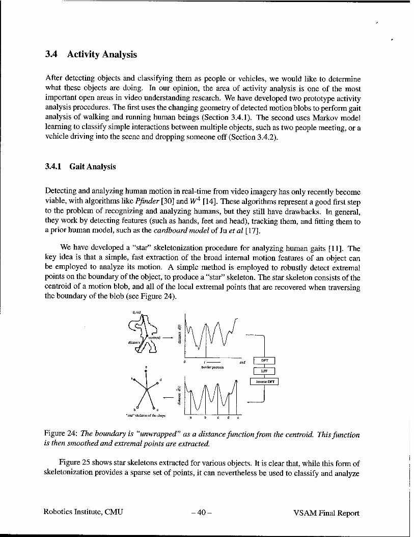
We have developed a "star" skeletonization procedure for analyzing human gaits [11]. The key idea is that a simple, fast extraction of the broad internal motion features of an object can be employed to analyze its motion. A simple method is employed to robustly detect extremal points on the boundary of the object, to produce a "star" skeleton. The star skeleton consists of the centroid of a motion blob, and all of the local extremal points that are recovered when traversing the boundary of the blob (see Figure 24).

"slar" skeleton of the shape c d e

Figure 24: The boundary is "unwrapped" as a distance function from the centroid. This function is then smoothed and extremal points are extracted.

Figure 25 shows star skeletons extracted for various objects. It is clear that, while this form of skeletonization provides a sparse set of points, it can nevertheless be used to classify and analyze


the motion of different types of moving object.

video image motion detection

(c) Polar bear

Figure 25: Skeletonization of different moving objects. It is clear the structure and rigidity of the skeleton is significant in analyzing object motion.

One technique often used to analyze the motion or gait of an individual is the cyclic motion of individual joint positions. However, in our implementation, the person may be a fairly small blob in the image, and individual joint positions cannot be determined in real-time, so a more fundamental cyclic analysis must be performed. Another cue to the gait of the object is its posture. Using only a metric based on the star skeleton, it is possible to determine the posture of a moving human. Figure 26 shows how these two properties are extracted from the skeleton. The uppermost skeleton segment is assumed to represent the torso, and the lower left segment is assumed to represent a leg, which can be analyzed for cyclic motion.

n

h.W -0- +

(a) (b)

Figure 26: Determination of skeleton features, (a) 0 is the angle the left cyclic point (leg) makes with the vertical, and (b) <|) is the angle the torso makes with the vertical.

Figure 27 shows human skeleton motion sequences for walking and running, and the values of 9„ for the cyclic point. This data was acquired from video at a frame rate of 8Hz. Comparing the average values (j)„ in Figures 27(e)-(f) shows that the posture of a running person can easily be


0.125 [sec] frame

kkk 1 kkA 1 kk 123456789 10

k \ \ kk \ \ kkk 11 12 13 14 15 16 17 18 19 20

(a) skeleton motion of a walking person

! \ k \ \ X \ X \ X 123456789 10

\ n \u UH 11 12 13 14 15 16 17 18 19 20

(b) skeleton motion of a running person

-0.5

-1

( T ( 1

10 15 frame

20 25

(c) leg angle 9 of a walking person (d) leg angle 0 of a running person

0 5 10. 15 20 25

(e) torso angle<(> of a walking person

0.4

„0.3

g0.2

0.1

o. '0 5 10, 15 20 25 frame

(f) torso angle <|> of a running person

Figure 27: Skeleton motion sequences. Clearly, the periodic motion of Qn provides cues to the object's motion as does the mean value oftyn.

distinguished from that of a walking person, using the angle of the torso segment as a guide. Also, the frequency of cyclic motion of the leg segments provides cues to the type of gait.

3.4.2 Activity Recognition of Multiple Objects using Markov Models

We have developed a prototype activity recognition method that estimates activities of multiple objects from attributes computed by low-level detection and tracking subsystems. The activity label chosen by the system is the one that maximizes the probability of observing the given attribute sequence. To obtain this, a Markov model is introduced that describes the probabilistic relations between attributes and activities.

We tested the functionality of our method with synthetic scenes which have human-vehicle interaction. In our test system, continuous feature vector output from the low-level detection and tracking algorithms is quantized into the following discrete set of attributes and values for each tracked blob


• object class: Human, Vehicle, HumanGroup

• object action: Appearing, Moving, Stopped, Disappearing

• Interaction: Near, MovingAwayFrom, MovingTowards, Nolnteraction

The activities to be labeled are 1) A Human entered a Vehicle, 2) A Human got out of a Vehicle, 3) A Human exited a Building, 4) A Human entered a Building, 5) A Vehicle parked, and 6) Human Rendezvous. To train the activity classifier, conditional and joint probabilities of attributes and actions are obtained by generating many synthetic activity occurrences in simulation, and measuring low-level feature vectors such as distance and velocity between objects, similarity of the object to each class category, and a noise-corrupted sequence of object action classifications. Figure 28 shows the results for two scenes that were not used for joint probability calculation.

*Be■'"* ||| | < J

' ! No

! NO

HrnnDapli ,'OU Hum Sttjij 200 JmG:Däp:ü.100

tear No N£3rnr Car Stp 0 800

Car:Dap:0.100 Hm'j.-Dao.O mn Mi

ResultO: A Human exited a Building Result 1: A Human entered a Vehicle

File JLLIJ

ResultO: A Vehicle parked Resultl: A Human got out of a Vehicle

Figure 28: Results of Markov activity recognition on synthetic scenes. Left: A person leaves a building and enters a vehicle. Right: A vehicle parks and a person gets out.

3.5 Web-page Data Summarization

We have developed a web-based data logging system (see Figure 29). In a high-traffic area, data on dozens of people can be collected in just a few minutes of observation. Each observation consists of color or thermal video from multiple cameras, best view image chips, collateral information such as date and time, weather conditions, temperature, estimated 3D subject trajectory, camera acquisition parameters, and object classification results. In addition to storing data for evaluation and debugging, a data logging system will be necessary when VSAM systems begin 24/7 site monitoring operation.

In our data logging prototype, all observations can be explored by web browsing via CGI through an HTTP server, so that VSAM researchers can access the data from anywhere. There are two ways to view object and activity information. Figure 30 shows a example activity report. The activity report shows labeled events such as a "Car Parked", or "A Human Entered a Building",

Robotics Institute, CMU ■43 VSAM Final Report

camera A

VSAM Database

Target Detection

Activity Monitoring

Activity Database

Target Classification

10:25 am A Human(#001) gor oui of a Vehicle(#002> 10:30 am A Vehicle pari;ed(#003) -»^_

C #001 Human red #002 Vehicle sedan Hue #003 Vehilce sedan red

,~*.#013 Human yellow

Figure 29: Web-page data summarization system.

sorted by time. If a user wants more detail, a hypertext link brings up a page showing an image chip of the object, along with its class and color information. Figure 31 shows an example object report. All of the objects seen by the system, and the activities to which they are related, are shown on a page, sorted by time of observation. To cut down on information overload, the user can select specific subsets of object classes to view. When the user selects an object, the system automatically brings up a page showing other objects of the same class having similar color features. In this way, it might be possible for a user to detect the same vehicle or person being observed at different places and times around the surveillance site.

A y 1 t .* ^ J if I j Ö«* • -.-'. ,M__i_ _(*»«* 5MX* NMmw P-H ;«u« - i

00:36:05 00:36:08 00:36:13 00:36:15 00:36:23 00:36:36 00:36:49 00:37:13 00:37:31

si'*öWtytB(wft):iafgä(gM&

Activity Report (Nov 9th 1999)

A Vehicle parked

A Vehicle parked

A Human got out of a Vehicle

A Human got out of a Vehicle

Human Rendezvous

A Human entered a Vehicle

A Human entered a Bidding

A Human ewted a Building

A Human entered a Vehicle

{select ActNity

Sedan

Sedan

Human. Sedai

Human. Sedan

Human. Human

Human. Sedan

Human

Human

Human, Sedan

ft* click-

aigää^g '.mmmmmm.

more detail

„ __ _ _ 9^m/o_puLioi9»tegi7001^(»1] __ a

VSAM 1 VS*MfSOO.jrt^rt ;en«t'fxm/tebMi^fr^mp^m H^^ÛBPi

TS(B«:«i;IJttt*. ;

i jMietB|;(H|(%g

Type: Human (11500.0), Human_G (1059.5). Mule (63.6) Col«: Wh,SI,Gy (4484.3), DBI,DGy,BI (2570.8), Rd.Or.Yl (692.3) Position: (202,59) on the right camera Capture time 00:36:19 PM

Type: Sedan (207.1), SVan,4WD (154.2), Human (100.0) Color: DRd,DOr(1155.6), DBI.DGy.BI(872.6), Wh.SI.Gy (196.6) Position: (253,70) on the right camera Capture time 00:36:04 PM

This page is maintained ov The Robdics InsniKa at Carnegie Melfcn University Please atttress comments to hircnobufiKs cmp edu

: 'Siiimi1?MMäääM!M$

Figure 30: Activity report for web page.

Robotics Institute, CMU •44- VSAM Final Report

E

1 ► click.

Tvset Report (Mw an«

j? " " 'Cl^-.rjätKw" ■

HPK Se*r (3051E). SVer..*» (873t). Wff J OH 8) C«Lsr Y*S.«» (11623). B JB (10S6 31. DOM*.» (412«)

■n (131 .87) on ÜB ft»! CMiM

T)!.* Hieran (II WO Oj.rieiir. 0|1«99.'**(6Se) Ugr V*S>.0y (4*6« 3). DrM», B. R57D B). Rd.0r.Y1 [«M 3)

search

... 6>ww*i^;/a#. - - i r \ > ; tut •- - Wa "mi;

pijiliffi^ fOagwafty«ariil.arujMâpffl /lOflîarq negB;M1 <

pfgäpSBi*

E tarä« ip:!<pT^SKä'iln*äf""

Type: Huron (11500.0), Human.G (1058.5). Mule (63.5) Color Wh,S,Gy (4464.3). DBI.DGy.BI (2570.8), Rd.0r.YI (692.3) PoeltJon: (202,56) on the right »men Capture time 00:36:16 PM

Type: Human (6500.0) Color Wh.S.Gy (2048.6). DBI,DQy,BI(1461.2). Rd.Or.YI (417.B) Poeition: (280.62) on the right camera Capture time 00:37:18 PM Activity: A Human exited a Bidding A Human entered a Vehicle

THE papa Is mninmlnad by TUB Robert« ftser.tt el Canada Mafcn Lrtwwsifr PIBBSB nimmw rommawsto Nroncbmacs cmu.odtJ

rf r.W«,tC»B ^SSki^MSS^

Figure 31: Object report for web page.

3.6 Airborne Surveillance

Fixed ground-sensor placement is fine for defensive monitoring of static facilities such as depots, warehouses or parking lots. In those cases, sensor placement can be planned in advance to get maximum usage of limited VSAM resources. However, the battlefield is a large and constantly shifting piece of real-estate, and it may be necessary to move sensors around in order to maximize their utility as the battle unfolds. While airborne sensor platforms directly address this concern, the self-motion of the aircraft itself introduces challenging video understanding issues. During the first two years of this program, the Sarnoff Corporation developed surveillance technology to detect and track individual vehicles from a moving aircraft, keep the camera turret fixated on a ground point, and multitask the camera between separate geodetic ground positions.

3.6.1 Airborne Object Tracking

Object detection and tracking is a difficult problem from a moving sensor platform. The difficulty arises from trying to detect small blocks of moving pixels representing independently moving object objects when the whole image is shifting due to self-motion. The key to success with the airborne sensor is characterization and removal of self-motion from the video sequence using the Pyramid Vision Technologies PVT-200 real-time video processor system. As new video frames stream in, the PVT processor registers and warps each new frame to a chosen reference image, resulting in a cancelation of pixel movement, and leading to a "stabilized" display that appears motionless for several seconds. During stabilization, the problem of moving object detection from a moving platform is ideally reduced to performing VSAM from a stationary camera, in the sense


that moving objects are readily apparent as moving pixels in the image. Object detection and tracking is then performed using three-frame differencing after using image alignment to register frame It-2 to It and frame It^\ to It, performed at 30 frames/sec. Sample results are shown in Figure 32. Under some circumstances, there is some remaining residual pixel motion due to parallax caused by significant 3D scene structure such as trees and smokestacks. Removing parallax effects is a subject of on-going research in the vision community.

Figure 32: Detection of small moving objects from a moving airborne sensor.

3.6.2 Camera Fixation and Aiming

It is well known that human operators fatigue rapidly when controlling cameras on moving airborne and ground platforms. This is because they must continually adjust the turret to keep it locked on a stationary or moving object. Additionally, the video is continuously moving, reflecting the self- motion of the camera. The combination of these factors often leads to operator confusion and nausea. Sarnoff has built image alignment techniques [5,13] to stabilize the view from the camera turret and to automate camera control, thereby significantly reducing the strain on the operator. In particular, real-time image alignment is used to keep the camera locked on a stationary or moving point in the scene, and to aim the camera at a known geodetic coordinate for which reference imagery is available. More details can be found in [28]. Figure 33 shows the performance of the stabilization/fixation algorithm on two ground points as the aircraft traverses an approximate ellipse over them. The field of view in these examples is 3°, and the aircraft took approximately 3 minutes to complete each orbit.

3.6.3 Air Sensor Multi-Tasking

Occasionally, a single camera resource must be used to track multiple moving objects, not all of which fit within a single field of view. This problem is particularly relevant for high-altitude air platforms that must have a narrow field of view in order to see ground objects at a reasonable


Fixation on target point A.

Fixation on target point B.

Figure 33: Fixation on two target points. The images shown are taken 0, 45, 90 and 135 seconds after fixation was started. The large center cross-hairs indicate the center of the stabilized image, i.e. the point of fixation

resolution. Sensor multi-tasking is employed to switch the field of view periodically between two (or more) target areas that are being monitored. This process is illustrated in Figure 34 and described in detail in [28].

Figure 34: Footprints of airborne sensor being autonomously multi-tasked between three disparate geodetic scene coordinates.

4 Site Models, Calibration and Geolocation

An automated surveillance system can benefit greatly from the scene-specific knowledge provided by a site model. Some of the many VSAM tasks supported by an accurate 3D site model are:

• computation of object geolocation (Section 4.3);


• visibility analysis (predicting what portions of the scene are visible from which cameras) to allow more effective sensor tasking;

• geometric focus of attention, for example to task a sensor to monitor the door of a building, or specify that vehicles should appear on roads;

• suppression of false alarms in areas of foliage;

• prediction of visual effects like shadows;

• visualization of the scene to enable quick comprehension of geometric relationships between sensors, objects, and scene features;

• simulation for planning best sensor placement and for debugging algorithms; and

• landmark-based camera calibration.

4.1 Scene Representations

Figure 35 illustrates the wide variety of scene representations that have been used in the VSAM testbed system over the past three years. Most of the variety is due to work in our first year of effort (1997), where we bootstrapped a representation of the Bushy Run site largely by hand. During the second and third years of the project, performed on the campus of CMU, we used a Compact Terrain Data Base (CTDB) model of campus, which ended up supporting almost all of our algorithmic needs.

A) USGS orthophoto. The United States Geological Survey (USGS) produces several digital mapping products that can be used to create an initial site model. These include 1) Digital Or- thophoto Quarter Quad (DOQQ) - a nadir (down-looking) image of the site as it would look under orthographic projection (Figure 35a). The result is an image where scene features appear in their correct horizontal positions. 2) Digital Elevation Model (DEM) - an image whose pixel values denote scene elevations at the corresponding horizontal positions. Each grid cell of the USGS DEM shown encompasses a 30-meter square area. 3) Digital Topographic Map (DRG) - a digital version of the popular USGS topo maps. 4) Digital Line Graph (DLG) - vector representations of public roadways and other cartographic features. Many of these can be ordered directly from the USGS EROS Data Center web site, located at URL ht tp: / / edcwww .cr.usgs. gov/. The ability to use existing mapping products from USGS or National Imagery and Mapping Agency (NIMA) to bootstrap a VSAM site model demonstrates that rapid deployment of VSAM systems to monitor trouble spots around the globe is a feasible goal.

B) Custom DEM. The Robotics Institute autonomous helicopter group mounted a high precision laser range finder onto a remote-control Yamaha helicopter to create a high-resolution (half-meter grid spacing) DEM of the Bushy Run site for VSAM DEMO I (Figure 35b). Raw radar returns were collected with respect to known helicopter position and orientation (using on-board altimetry data) to form a cloud of points representing returns from surfaces in the scene. These points were converted into a DEM by projecting into LVCS horizontal-coordinate bins, and computing the mean and standard deviation of height values in each bin.


Figure 35: A variety of site model representations have been used in the VSAMIFD testbed system: A) USGS orthophoto; B) custom DEM; C) aerial mosaic; D) VRML model; E) CTDB site model; andF) spherical representations.


C) Mosaics. A central challenge in surveillance is how to present sensor information to a human operator. The relatively narrow field of view presented by each sensor makes it very difficult for the operator to maintain a sense of context outside the camera's immediate image. Image mosaics from moving cameras overcome this problem by providing extended views of regions swept over by the camera. Figure 35c displays an aerial mosaic of the Demo I Bushy Run site. The video sequence was obtained by flying over the demo site while panning the camera turret back and forth and keeping the camera tilt constant[13, 25, 24]. The VSAM IFD team also demonstrated coarse registration of this mosaic with a USGS orthophoto using a projective warp to determine an approximate mapping from mosaic pixels to geographic coordinates. It is feasible that this technology could lead to automated methods for updating existing orthophoto information using fresh imagery from a recent fly-through. For example, seasonal variations such as fresh snowfall (as in the case of VSAM Demo I) can be integrated into the orthophoto.

D) VRML models. Figure 35d shows a VRML model of one of the Bushy Run buildings and its surrounding terrain. This model was created by the K2T company using the factorization method [26] applied to aerial and ground-based video sequences.

E) Compact Terrain Data Base (CTDB). During the last two years, the VSAM testbed system has used a Compact Terrain Data Base (CTDB) model of campus as its primary site model representation. The CTDB was originally designed to represent large expanses of terrain within the context of advanced distributed simulation, and has been optimized to efficiently answer geometric queries such as finding the elevation at a point in real-time. Terrain can be represented as either a grid of elevations, or as a Triangulated Irregular Network (TIN), and hybrid data bases containing both representations are allowed. The CTDB also represents relevant cartographic features on top of the terrain skin, including buildings, roads, bodies of water, and tree canopies. Figure 35e shows a small portion of the Schenley Park / CMU campus CTDB. An important benefit to using CTDB as a site model representation for VSAM processing is that it allows us to easily interface with the synthetic environment simulation and visualization tools provided by ModSAF and ModStealth.

F) Spherical Representations. During the second year (1998), VSAM testbed SPU's used the Microsoft Windows NT operating system, which is not supported by CTDB software. For that reason, we explored the use of spherical lookup tables for each fixed-mount SPU. Everything that can be seen from a stationary camera can be represented on the surface of a viewing sphere (Figure 35f). This is true even if the camera is allowed to pan and tilt about the focal point, and to zoom in and out - the image at any given (pan,tilt,zoom) setting is essentially a discrete sample of the bundle of light rays impinging on the camera's focal point. We used this idea to precompile and store a spherical lookup table containing the 3D locations and surface material types of the points of intersection of camera viewing rays with the CTDB site model. During the third year, we changed from Windows to the Linux operating system, a variant of Unix, and could then use CTDB directly on each SPU. This made the spherical lookup tables obsolete.

Three geospatial site coordinate systems are used interchangeably within the VSAM testbed. The WGS84 geodetic coordinate system provides a reference frame that is standard, unambiguous and global (in the true sense of the word). Unfortunately, even simple computations such as the


distance between two points become complicated as a function of latitude, longitude and elevation. For this reason, site-specific Cartesian coordinate systems are typically established to handle the bulk of the geometric model computations that must be performed. We have used a Local Vertical Coordinate System (LVCS) [2] with its origin at the base of the PRB operator control center for representing camera positions and for providing an operator display map coordinate system. The CTDB model of campus is based on Universal Transverse Mercator (UTM) coordinates, which provide an alternative Cartesian coordinate system, and which are related to the LVCS by a rotation and translation. Conversion between geodetic, LVCS, and UTM coordinates is straightforward, so that each can be used interchangeably in the system.

4.2 Camera Calibration

For a VSAM system to make full use of a geometric site model requires calibrating the cameras with respect to the model. We have developed a set of calibration procedures specifically designed for in-situ (meaning "in place") camera calibration. We believe that all cameras should be calibrated in an environment that resembles their actual operating conditions. This philosophy is particularly relevant for outdoor camera systems. Cameras get jostled during transport and installation, and changes in temperature and humidity can affect a camera's intrinsic parameters. Furthermore, it is impossible to recreate the full range of zoom and focus settings that are useful to an outdoor camera system within the confines of an indoor lab.

Some amount of on-site calibration is always necessary, if only for determining the extrinsic parameters (location and orientation) of the camera placement. Unfortunately, outdoors is not an ideal environment for careful camera calibration. It can be cold, rainy, or otherwise unpleasant. Simple calibration methods are needed that can be performed with minimal human intervention.

Figure 36: GPS landmarks measurements for extrinsic camera calibration on the CMU campus.


We have developed methods for fitting a projection model consisting of intrinsic (lens) and extrinsic (pose) parameters of a camera with active pan, tilt and zoom control. Intrinsic parameters are calibrated by fitting parametric models to the optic flow induced by rotating and zooming the camera. These calibration procedures are fully automatic and do not require precise knowledge of 3D scene structure. Extrinsic parameters are calculated by sighting a sparse set of measured landmarks in the scene (see Figure 36). Actively rotating the camera to measure landmarks over a virtual hemispherical field of view leads to a well-conditioned exterior orientation estimation problem. Details of the calibration procedures are presented in [8].

4.3 Model-based Geolocation

The video understanding techniques described in Section 3 operate primarily in image space. A large leap in terms of descriptive power can be made by transforming image blobs and measurements into 3D scene-based objects and descriptors. In particular, determination of object location in the scene allows us to infer the proper spatial relationships between sets of objects, and between objects and scene features such as roads and buildings. Furthermore, we believe that computation of 3D spatial geolocation is the key to coherently integrating a large number of object hypotheses from multiple, widely-spaced sensors.

User view

-1 *&•'•;

Ray: (XO,Y0,2O) + k(U,V,W)

|^5jxo, YO, ZO

v p

, l S ertical 1 ^<8C rojection | ^^ 3|

w ■f

TV

1 I 1 1 1 1 1 °^j ay: (XO.YO) + k(U,V) -

4

3 2

1 V

^J X0.Y0 9 8^*

7 6

12 \Y\p 10

13 f Elev( XO+kU, YO+kV) > ZO + kW

(a) (b)

Figure 37: (a) Estimating object geolocations by intersecting backprojected viewing rays with a terrain model, (b) A Bresenham-like traversal algorithm determines which DEM cell contains the first intersection of a viewing ray and the terrain.

In regions where multiple sensor viewpoints overlap, object locations can be determined very accurately by wide-baseline stereo triangulation. However, regions of the scene that can be simul-


taneously viewed by multiple sensors are likely to be a small percentage of the total area of regard in real outdoor surveillance applications, where it is desirable to maximize coverage of a large area using finite sensor resources. Determining object locations from a single sensor requires domain constraints, in this case the assumption that the object is in contact with the terrain. This contact location is estimated by passing a viewing ray through the bottom of the object in the image and intersecting it with a model representing the terrain (see Figure 37a). Sequences of location estimates over time are then assembled into consistent object trajectories.

Previous uses of the ray intersection technique for object localization in surveillance research have been restricted to small areas of planar terrain, where the relation between image pixels and terrain locations is a simple 2D homography [6, 10, 20]. This has the benefit that no camera calibration is required to determine the back-projection of an image point onto the scene plane, provided the mappings of at least four coplanar scene points are known beforehand. However, large outdoor scene areas may contain significantly varied terrain. To handle this situation, we perform geolocation using ray intersection with a full terrain model provided, for example, by a digital elevation map (DEM).

Given a calibrated sensor, and an image pixel corresponding to the assumed contact point between an object and the terrain, a viewing ray (*o + ku,yo + kv,zo + kw) is constructed, where (xo,yo,zo) is the 3D sensor location, (w, v, w) is a unit vector designating the direction of the viewing ray emanating from the sensor, and k > 0 is an arbitrary distance. General methods for determining where a viewing ray first intersects a 3D scene (for example, ray tracing) can be quite involved. However, when scene structure is stored as a DEM, a simple geometric traversal algorithm suggests itself, based on the well-known Bresenham algorithm for drawing digital line segments. Consider the vertical projection of the viewing ray onto the DEM grid (see Figure 37b). Starting at the grid cell (jto,yo) containing the sensor, each cell (x,y) that the ray passes through is examined in turn, progressing outward, until the elevation stored in that DEM cell exceeds the z-component of the 3D viewing ray at that location. The z-component of the view ray at location (x,y) is computed as either

, (*-*ö) , (y-yo) /ox Z0+- -w or zoH w (9)

U V

depending on which direction cosine, u or v, is larger. This approach to viewing ray intersection localizes objects to lie within the boundaries of a single DEM grid cell. A more precise sub-cell location estimate can then be obtained by interpolation. If multiple intersections with the terrain beyond the first are required, this algorithm can be used to generate them in order of increasing distance from the sensor, out to some cut-off distance. See [7] for more details.

Geolocation Evaluation

We have evaluated geolocation accuracy for two cameras (PRB and Wean) on the CMU campus using a Leica laser-tracking theodolite to generate ground truth. The experiment was run by having a person carry the theodolite prism for two loops around the PRB parking lot, while the system logged time-stamped horizontal (X,Y) positions estimated by the Leica theodolite. The


system also simultaneously tracked the person using the PRB and Wean cameras, while logging time-stamped geolocation estimates from each camera.

aj^se™.-:! mn, •«.«iSKKBy

r.3 . ̂ j^j||£

hi 2480 °

A S *W00> 2470 \ '

UP^fe'

2460

2450 ^-, 1 w>. fyr-mgSf, 1510 1520 1530

tSffff" "' "* " 2480

it Swap' , 2470

• ' *,

2450

III

1490 1500 1510 1520

(a) (b)

Figure 38: Ground truth trajectory overlaid with geolocation estimates from a) PRB camera, b) Wean camera, and c) an average of PRB and Wean estimates. Scales are in meters.

Figure 38 shows the ground truth trajectory curve, overlaid with geolocation estimates from (a) the PRB camera, (b) the Wean camera, and (c) an average of the PRB and Wean camera estimates for corresponding time stamps. Both cameras track the overall trajectory fairly well. The PRB camera geolocation estimates have large errors at the lower portions and upper right arc of the loop, because the person's feet were occluded by parked vehicles when walking through those areas. The higher elevation and direction of view of Wean camera allowed it to see the person's feet at the lower portion of the loop, so the trajectory is correctly followed there. An error still occurs at the top right of the loop, as the person comes close to two vehicles and is reflected from their shiny surfaces. This pulls the bounding box off the person's feet, and causes an underestimation of their position. Geolocation estimates were only averaged for points with time stamps agreeing to within a small threshold, so there are far fewer points shown in Figure 38c. The effect of averaging is to smooth out many of the high variance portions of both curves, although the overall distance accuracy does not noticeably improve.

Geolocation estimates are computed by backprojecting a point located at the center of the lowest side of the bounding box enclosing a moving blob. The system maintains a running estimate of the variance of this point - the variance is high when the position or shape of the bounding box changes greatly during tracking. The system computes an internal estimate of horizontal geolocation error by projecting an error box of one standard deviation around the image point used for estimation, until it intersects the terrain, thus providing a bound on the error of the geolocation estimate. A subsampling of this set of error boxes is shown in Figure 39, for both cameras. It is interesting to note that during portions of the trajectory where errors are large due to occlusions or reflections, the system is aware that the variance of the geolocation estimate is high.

To determine actual geolocation accuracy, the time stamp of each geolocation estimate was compared to the list of ground truth time stamps to find a suitably close correspondence. For cases where a corresponding ground truth point was found, the horizontal displacement error is plotted in Figure 40, for a) PRB camera, b) Wean camera, and c) the average geolocation computed from PRB and Wean. The mean and covariance of each point cloud were estimated, and the major and


s* ^ 2480

2470 0 ****

2460

2450 i j> ^W 1500 1510 1520 1530 1540

(a)

Figure 39: Geolocation error boxes computed by the system for trajectory estimates from a) PRB camera and b) Wean camera. Scales are in meters. Compare with Figures 38a and b.

minor axes of the covariance ellipse is overlaid on each plot, with the length of the axes scaled to represent 1.5 times the standard deviation of the point spread along that direction. Numeric standard deviations along each axis are displayed in the following table.

Geolocation Estimates max std (meters) min std (meters) PRB Wean Avg of PRB and Wean

0.6520 0.5232 0.7184

0.3139 0.1628 0.3337

These numbers confirm the observation that averaging geolocation estimates from both cameras is not improving accuracy. It is actually getting slightly worse. Referring again to Figure 40, we see that the center of each error point spread is not at (0,0). We are therefore averaging biased geolocation estimates from each camera, and the noise in each estimate is therefore not cancelling out properly, but rather intensifying. Removing the geolocation bias from each sensor will be necessary to achieve more accurate results from averaging. Possible sources of error are the camera calibration parameters, the terrain model, and small biases in the time stamps produced by each SPU. Nonetheless, standard deviation of geolocation estimates from each camera are roughly on the order of .6 meters along the axis of maximum spread, and roughly .25 meters at minimum. We have confirmed that the axis of maximum error for each camera is oriented along the direction vector from the camera to the object being observed.

4.4 Model-based Human-Computer Interface

Keeping track of people, vehicles, and their interactions, over a chaotic area such as the battlefield, is a difficult task. The commander obviously shouldn't be looking at two dozen screens showing


2

1

*'^\

0

**' f " -1 '

-10 12 3

(a) (b)

Figure 40: Plotted covariances of the horizontal displacement errors between estimate geolocations and ground truth locations for corresponding time stamps, a) PRB camera, b) Wean camera, and c) average of PRB and Wean estimates with corresponding time stamps. Scales are in meters.

raw video output - that amount of sensory overload virtually guarantees that information will be ignored, and requires a prohibitive amount of transmission bandwidth. Our suggested approach is to provide an interactive, graphical visualization of the battlefield by using VSAM technology to automatically place dynamic agents representing people and vehicles into a synthetic view of the environment.

This approach has the benefit that visualization of the object is no longer tied to the original resolution and viewpoint of the video sensor, since a synthetic replay of the dynamic events can be constructed using high-resolution, texture-mapped graphics, from any perspective. Particularly striking is the amount of data compression that can be achieved by transmitting only symbolic geo- registered object information back to the operator control unit instead of raw video data. Currently, we can process NTSC color imagery with a frame size of 320x240 pixels at 10 frames per second on a Pentium II computer, so that data is streaming into the system through each sensor at a rate of roughly 2.3Mb per second per sensor. After VSAM processing, detected object hypotheses contain information about object type, location and velocity, as well as measurement statistics such as a time stamp and a description of the sensor (current pan, tilt, and zoom for example). Each object data packet takes up roughly 50 bytes. If a sensor tracks 3 objects for one second at 10 frames per second, it ends up transmitting 1500 bytes back to the OCU, well over a thousandfold reduction in data bandwidth.

Ultimately, the key to comprehending large-scale, multi-agent events is a full, 3D immersive visualization that allows the human operator to fly at will through the environment to view dynamic events unfolding in real-time from any viewpoint. We envision a graphical user interface based on cartographic modeling and visualization tools developed within the Synthetic Environments (SE) community. The site model used for model-based VSAM processing and visualization is represented using the Compact Terrain Database (CTDB). Objects are inserted as dynamic agents within the site model and viewed by Distributed Interactive Simulation clients such as the Modular Semi-Automated Forces (ModS AF) program and the associated 3D immersive ModStealth viewer.

We first demonstrated proof-of-concept of this idea at the Dismounted Battle Space Battle


Lab (DBBL) Simulation Center at Fort Benning Georgia as part of the April 1998 VSAM workshop. On April 13, researchers from CMU set up a portable VSAM system at the Benning Mobile Operations in Urban Terrain (MOUT) training site. The camera was set up at the corner of a building roof whose geodetic coordinates had been measured by a previous survey [12], and the height of the camera above that known location was measured. The camera was mounted on a pan-tilt head, which in turn was mounted on a leveled tripod, thus fixing the roll and tilt angles of the pan-tilt-sensor assembly to be zero. The yaw angle (horizontal orientation) of the sensor assembly was measured by sighting through a digital compass. After processing several troop exercises, log files containing camera calibration information and object hypothesis data packets were sent by FTP back to CMU and processed using the CTDB to determine a time-stamped list of moving objects and their geolocations. Later in the week, this information was brought back to the DBBL Simulation Center at Benning where, with the assistance of colleagues from BDM, it was played back for VSAM workshop attendees using custom software that broadcast time-sequenced simu- lated entity packets to the network for display by both ModSAF and ModStealth. Some processed VSAM video data and screen dumps of the resulting synthetic environment playbacks are shown in Figure 41.

Figure 41: Sample synthetic environment visualizations of data collected at the Benning MOUT site. A) Automated tracking of three people. B) ModSAF 2D orthographic map display of estimated geolocations. C) Tracking of a soldier walking out of town. D) Immersive, texture-mapped 3D visualization of the same event, seen from a user-specified viewpoint.

We have also demonstrated that this visualization process can form the basis for a real-time immersive visualization tool. First, we ported object geolocation computation using the CTDB onto the VSAM SPU platforms. This allowed estimates of object geolocation to be computed within the frame-to-frame tracking process, and to be transmitted in data packets back to the OCU. At the OCU, incoming object identity and geolocation data is repackaged into Distributed Inter- active Simulation (DIS) packets understood by ModSAF and ModStealth clients, and re-broadcast (multicast) on the network. At that point, objects detected by the SPUs are viewable, after a short lag, within the context of the full 3D site model using the ModStealth viewer (Figure 42).

Robotics Institute, CMU •57 VSAM Final Report

Figure 42: Real-time, 3D ModStealth visualization of objects detected and classified by the VSAM testbed system and transmitted via DJS packets on the network.

5 Sensor Coordination

In most complex outdoor scenes, it is impossible for a single sensor to maintain its view of an object for long periods of time. Objects become occluded by environmental features such as trees and buildings, and sensors have limited effective fields of regard. A promising solution to this problem is to use a network of video sensors to cooperatively track objects through the scene. We have developed and demonstrated two methods of sensor coordination in the VSAM testbed. First, objects are tracked long distances through occlusion by handing-offbetween cameras situated along the object's trajectory. Second, wide-angle sensors keeping track of all objects in a large area are used to task active pan, tilt and zoom sensors to get a better view of selected objects, using a process known as sensor slaving.

5.1 Multi-Sensor Handoff

There has been little work done on autonomously coordinating multiple active video sensors to cooperatively track a moving object. One approach is presented by Matsuyama for a controlled indoor environment where four cameras lock onto onto a particular object moving across the floor [23]. We approach the problem more generally by using the object's 3D geolocation (as computed in the last section) to determine where each sensor should look. The pan, tilt and zoom of the closest sensors are then controlled to bring the object within their fields of view, while a viewpoint independent cost function is used to determine which of the moving objects they find are the specific object of interest. These steps are described below.

Assume that at time t0 a sensor with pan, tilt value (60, §o) has been tasked to track a particular object with 3D ground location X0 and velocity X. Given a function G(X) that converts a ground coordinate to a pan, tilt point (determined by camera calibration), the object's location X0

is converted to a desired sensor pan, tilt value (Qd, <$>d) = G(X0). The behavior of the pan, tilt unit


is approximated by a linear system with infinite acceleration and maximum velocity (±9, ±<j>) as

B(t) = Qo±B(t-to) (m

Substituting the desired sensor pan, tilt (Qj, fa) into the left hand side of this equation and solving for (t - to) yields a prediction of the acquisition time, that is, how long it would take for the pan, tilt device to point at the object's current location. However, the object will have moved further along its trajectory by that time. This new object position is estimated as

X(t)=Xo+X(t-to) (11)

This predicted object position is then converted into a new desired sensor pan, tilt, and the whole procedure iterates until the time increments (t - to) become small (convergence) or start to increase (divergence). This algorithm guarantees that if it converges, the sensor will be able to reacquire the object.

An appropriate camera zoom setting can be determined directly given a desired size of the object's projection in the image. Knowing the classification of the object C (as determined from Section 3.3), we employ the heuristic that humans are approximately 6 feet (2m) tall and vehicles are approximately 15 feet (5m) long. Given the position of the object and the sensor, and therefore the range r to the object, the angle p subtended by the image of the object is approximately

{ tan 1 ^, human tan-1 4, vehicle

Knowing the focal length of the sensor as a function of zoom, as determined from camera calibration, the appropriate zoom setting is easily chosen.

Once the sensor is pointing in the right direction at the right zoom factor, all moving objects extracted are compared to the specific object of interest to see if they match. This need to re-acquire a specific object is a key feature necessary for multi-camera cooperative surveillance. Obviously viewpoint-specific appearance criteria are not useful, since the new view of the object may be significantly different from the previous view. Therefore, recognition features are needed that are independent of viewpoint. In our work we use two such criteria: the object's 3D scene trajectory as determined from geolocation, and a normalized color histogram of the object's image region. Candidate motion regions are tested by applying a matching cost function in a manner similar to that described in Section 3.2.

An example of using multi-sensor hand-off to track a vehicle as it travels through campus is shown in Figure 43. This diagram shows the continuous, autonomous tracking of a single object for a distance of approximately 400m and a time of approximately 3 minutes. In Figure 43(a) two sensors cooperatively track the object. At the time shown in Figure 43(b) the object is occluded from sensor 2, but is still visible from sensor 1, which continues to track it. When the object moves out of the occlusion area, sensor 2 is automatically retasked to track it, as shown in Figure 43(c).


Sensor - view fijFM

■ Sensor 1- view

Figure 43: Cooperative, multi-sensor tracking (see text for description).


Finally, when the object moves out of the field of regard of both sensors, a third sensor is automatically tasked to continue surveillance, as shown in Figure 43(d). By automatically managing multiple, redundant camera resources, the vehicle is continuously tracked through a complex urban environment.

5.2 Sensor Slaving

A second form of sensor cooperation is sensor slaving. We use the term sensor slaving to denote using one wide field of view camera to control a second, active camera to zoom in and actively follow the subject to generate a better view. The motivation is to keep track of all objects in the scene while simultaneously gathering high-resolution views of selected objects. A camera slaving system has at least one master camera and one slave camera. The master camera is set to have a global view of the scene so that it can track objects over extended areas using simple tracking methods such as adaptive background subtraction. The object trajectory generated by the master camera is relayed to the slave camera in real time. The slave camera, which is highly zoomed in, can then follow the trajectory to generate close-up imagery of the object.

Slaving is a relatively simple exercise if both cameras are calibrated with respect to a local 3D terrain model. We have shown in Section 4.3 that a person's 3D trajectory can be determined to reasonable accuracy (roughly 1 meter of error for a person 50 meters away) by intersecting backprojected viewing rays with the terrain. After estimating the 3D location of a person from the first camera's viewpoint, it is an easy matter to transform the location into a pan-tilt command to control the second camera. Figure 44 shows an example of camera slaving. A person has been detected automatically in the wide-angle view shown in the left image, and a second camera has been tasked to move slightly ahead of the person's estimated 3D trajectory, as shown in the right image.

For cameras located far apart geographically, it is obvious that we need to have very good camera calibration, and an accurate 3D site model. We have also developed a sensor slaving method that works for closely located cameras. This method requires only image-based computations (no geolocation computation or extrinsic camera calibration). Furthermore, intrinsic parameters are needed only by the slave camera, which has to determine the pan/tilt angles needed to point towards each pixel in the image. The basic idea is to form a mosaic by warping the master camera view into the pixel coordinate system of the slave camera view (Figure 45). Image trajectories of objects detected in the master view can then be transformed into trajectories overlaid on the slave camera view. The slave camera can then compute the pan-tilt angles necessary to keep the object within its zoomed field of view.


Figure 44: Example of camera slaving. Left: wide-angle view in which a person is detected. Right: a better view from a second camera, which has been tasked to intercept the person's estimated 3D path.

Figure 45: (a) and (b) are images taken from a slave camera and master camera, respectively, (c) shows the master camera view warped into the pixel coordinate system of the slave camera view, to form an image mosaic. Image pixels are averaged directly in overlapping region.


6 Three Years of VSAM Milestones

The current VSAM IFD testbed system and suite of video understanding technologies are the end result of a three-year, evolutionary process. Impetus for this evolution was provided by a series of yearly demonstrations. The following tables provide a succinct synopsis of the progress made during the last three years in the areas of video understanding technology, VSAM testbed architecture, sensor control algorithms, and degree of user interaction.

Although the program is over now, the VSAM IFD testbed continues to provide a valuable resource for the development and testing of new video understanding capabilities. Future work will be directed towards achieving the following goals:

• better understanding of human motion, including segmentation and tracking of articulated body parts;

• improved data logging and retrieval mechanisms to support 24/7 system operations;

• bootstrapping functional site models through passive observation of scene activities;

• better detection and classification of multi-agent events and activities;

• better camera control to enable smooth object tracking at high zoom; and

• acquisition and selection of "best views" with the eventual goal of recognizing individuals in the scene.


Table 3: Progression of Video Understanding Technology Video Understanding 1997 Demo Results 1998 Demo Results 1999 Demo Results Ground-based moving target detection (MTD) and tracking

Multiple target detection, single target step and stare tracking, temporal change, adaptive template matching

Multi-target MTD and trajectory analysis, motion salience via temporal consistency, adaptive background subtraction

Layered and adaptive background subtraction for robust detection, MTD while panning, tilting and zooming using optic flow and image registration, target tracking by multi-hypothesis Kaiman filter

Airborne MTD and tracking

Stabilization / temporal change using correlation

Real-time camera pointing based on motion plus appearance, drift free fixation

(N/A)

Ground-based target geolocation

Ray intersection with DEM Ray intersection with SEEDS model

Geolocation uncertainty estimation by Kaiman filtering, domain knowledge

Airborne target geolocation

Video to reference image registration

Fine aiming using video to reference image registration in real-time

(N/A)

Target recognition Temporal salience (predicted trajectory)

Spatio-temporal salience, color histogram, classification

Target patterns and/or spatio-temporal signature

Target classification technique

Aspect ratio Dispersedness, motion-based skeletonization, neural network, spatio-temporal salience

Patterns inside image chips, spurious motion rejection, model-based recognition, Linear Discriminant Analysis

Target classification categories

Human, vehicle Human, human group, vehicle

Human, human group, sedan, van, truck, mule, FedEx van, UPS van, police car

Target classification accuracy (percentage correctly identified)

87% Vehicle, 83% Human (small sample)

85% (large sample) > 90% (large sample)

Activity monitoring Any motion Individual target behaviors Multiple target behaviors: parking lot monitoring, getting in/out of cars, entering buildings

Ground truth verification

None Off-line On-line (one target)

Geolocation accuracy 5 meters 2 meters < 1 meter Camera calibration Tens of pixels Fives of pixels Ones of pixels Domain knowledge Elevation map and

hand-drawn road network SEEDS model used to generate ray occlusion tables off-line

Parking area, road network, occlusion boundaries


Table 4: Progression of VSAM Architecture Goals VSÄM Architecture 1997 Demo Results 1998 Demo Results 1999 Demo Results

Number of SPUs 3 8 12

Types of Sensors Standard video camera with fixed focal length

Standard video camera with zoom, omnicamera

Static color and B/W cameras, color video cameras with pan, tilt and zoom, omnicamera, thermal

Types of SPU and VSAM nodes

Slow relocatable, airborne Fast relocatable, fixed-mount, airborne, visualization clients

Super-SPU handling multiple cameras, web-based VIS-node

System coverage Rural, 0.1 km2 area ground-based, 3 km2

airborne coverage

University campus, 0.3 km2

area ground-based, airborne coverage over 9 km2 urban area

Dense coverage of university campus, 0.3km2 ground-based area of interest

Communcation architecture

Dedicated OCU/SPU Variable-packet protocol

Table 5: Progression of VSAM Sensor Control Sensor Control 1997 Demo Results 1998 Demo Results 1999 Demo Results

Ground sensor aiming (hand-off and multitasking)

Predetermined handoff regions

3D coordinates and signatures, epipolar constraints, occlusion and footprint databases

Camera-to-camera handoff, wide-angle slaving

Air sensor aiming Video to reference image registration for landmark points

Video to reference image registration for landmark points

(N/A)

Ground / Air interaction

Human-directed to predetermined locations

OCU-directed to target geolocation

(N/A)

SPU behavior Single supervised task (track target) with primitive unsupervised behavior (look for target)

Single-task supervision (track activity) with unsupervised behavior (loiter detection)

Multi-task supervision for activity monitoring and complex unsupervised behavior (parking lot monitoring)

Robotics Institute, CMU -65- VS AM Final Report

Table 6: Progression of User Interaction User Interaction 1997 Demo Results 1998 Demo Results 1999 Demo Results

Site model USGS orthophoto and DEM, LIDAR, real-time mosaics

Compact Terrain DataBase (CTDB), spherical mosaics, aerial mosaic

Improved CTDB model

Site model function Visualization and geolocation

Off-line: Demo scenario planning, after-action review, algorithm evaluation, ground-truth verification. On-line: Relocatable sensor planning and geolocation, occlusion analysis, target geolocation

Off-line: Sensor placement and planning, virtual SPU for scenario perturbation analysis. On-line: Ground-truth verification, dynamic visualization and system tasking

System tasking by user (user interface)

2D point-and-click camera control for sensor-based tasking

2D point-and-click camera control for region and target-based tasking.

Tracked-object specification, 3D interactive activity and event-based tasking

Visualization Overlay current target and sensor positions on orthophoto, live video feeds

Target and sensor information shown on GUI display, computer switchable live video feeds, ModStealth

ModStealth visualization of sensor network, video archiving and replaying of significant events

WebVSAM None Java-based visualization nodes

Indexed web access to activity report, live internet access to VSAM network via Web visualization nodes


Acknowledgments

The authors would like to thank the U.S. Army Night Vision and Electronic Sensors Directorate Lab team at Davison Airfield, Ft. Belvoir, Virginia for their help with the airborne operations. We would also like to thank Chris Kearns and Andrew Fowles for their assistance at the Fort Benning MOUT site, and Steve Haes and Joe Findley at BDM/TEC for their help with the the CTDB site model and distributed simulation visualization software.

References

[1] C. Anderson, Peter Burt, and G. van der Wal. Change detection and tracking using pyramid transformation techniques. In Proceedings ofSPIE - Intelligent Robots and Computer Vision, volume 579, pages 72-78,1985.

[2] American Society of Photogrammetry ASP. Manual of Photogrammetry. Fourth Edition, American Society of Photogrammetry, Falls Church, 1980.

[3] Y. Bar-Shalom and T. Fortmann. Tracking and data association. Academic Press, Boston, 1988.

[4] J. Barron, D. Fleet, and S. Beauchemin. Performance of optical flow techniques. Interna- tional Journal of Computer Vision, 12(l):42-77, 1994.

[5] J. Bergen, P. Anandan, K. Hanna, and R. Hingorani. Hierarchical model-based motion estimation. In Proceedings of the European Conference on Computer Vision, 1992.

[6] K. Bradshaw, I. Reid, and D. Murray. The active recovery of 3d motion trajectories and their use in prediction. IEEE Transactions on Pattern Analysis and Machine Intelligence, 19(3):219-234, March 1997.

[7] R. Collins, Y. Tsin, J.R. Miller, and A. Lipton. Using a DEM to determine geospatial object trajectories. In Proceedings of the 1998 DARPA Image Understanding Workshop, pages 115- 122, November 1998.

[8] R.T. Collins and Y. Tsin. Calibration of an outdoor active camera system. In Proceedings of the 1999 Conference on Computer Vision and Pattern Recognition, pages 528-534. IEEE Computer Society, June 1999.

[9] F Dellaert and R.T. Collins. Fast image-based tracking by selective pixel integration. In ICCV99 Workshop on Frame-Rate Applications, September 1999.

[10] B. Flinchbaugh and T. Bannon. Autonomous scene monitoring system. In Proc. 10th Annual Joint Government-Industry Security Technology Symposium. American Defense Prepared- ness Association, June 1994.


[11] H. Fujiyoshi and A. Lipton. Real-time human motion analysis by image skeletonization. In Proceedings of the 1998 Workshop on Applications of Computer Vision, 1998.

[12] Geometric Geodesy Branch GGB. Geodetic Survey. Publication SMWD3-96-022, Phase II, Interim Terrain Data, Fort Benning, Georgia, May 1996.

[13] M. Hansen, P. Anandan, K. Dana, G. van der Wal, and P. Burt. Real-time scene stabilization and mosaic construction. In Proc. Workshop on Applications of Computer Vision, 1994.

[14] I. Haritaoglu, Larry S. Davis, and D. Harwood. W4 who? when? where? what? a real time system for detecing and tracking people. In FGR98,1998.

[15] M. Isard and A. Blake. Contour tracking by stochastic propagation of conditional density. In Proceedings of the 1996 European Conference on Computer Vision, pages 343-356,1996.

[16] Institute for Simulation & Training 1ST. Standard for Distributed Interactive Simulation - Application Protocols, Version 2.0. University of Central Florida, Division of Sponsored Research, March 1994.

[17] S. Ju, M. Black, and Y. Yacoob. Cardboard people: A parameterized model of articulated image motion. In Proceedings of International Conference on Face and Gesture Analysis, 1996.

[18] T. Kanade, R. Collins, A. Lipton, P. Anandan, and P. Burt. Cooperative multisensor video surveillance. In Proceedings of the 1997 DARPA Image Understanding Workshop, volume 1, pages 3-10, May 1997.

[19] T. Kanade, R. Collins, A. Lipton, P. Burt, and L. Wixson. Advances in cooperative multisensor video surveillance. In Proceedings of the 1998 DARPA Image Understanding Work- shop, volume 1, pages 3-24, November 1998.

[20] D. Koller, K. Daniilidis, and H. Nagel. Model-based object tracking in monocular image sequences of road traffic scenes. International Journal of Computer Vision, 10(3):257-281, June 1993.

[21] A. Lipton, H. Fujiyoshi, and R.S. Patil. Moving target detection and classification from real- time video. In Proceedings of the 1998 Workshop on Applications of Computer Vision, 1998.

[22] Alan J. Lipton. Local application of optic flow to analyse rigid versus non-rigid motion. In ICCV99 Workshop on Frame-Rate Applications, September 1999.

[23] T. Matsuyama. Cooperative distributed vision. In Proceedings of DARPA Image Understand- ing Workshop, volume 1, pages 365-384, November 1998.

[24] H. S. Sawhney, S. Hsu, and R. Kumar. Robust video mosaicing through topology inference and local to global alignment. In Proc. European Conference on Computer Vision, 1998.


[25] H. S. Sawhney and R. Kumar. True multi-image alignment and its application to mosaicing and lens distortion. In Proc. IEEE Conference on Computer Vision and Pattern Recognition, 1997.

[26] C. Tomasi and T. Kanade. Shape and motion from image streams: factorization method. International Journal of Computer Vision, 9(2), 1992.

[27] K. Toyama, J. Krumm, B. Brumitt, and B. Meyers. Wallflower: Principles and practice of background maintenance. In Proc. International Conference on Computer Vision, pages 255-261,1999.

[28] L. Wixson, J. Eledath, M. Hansen, R. Mandelbaum, and D. Mishra. Image alignment for precise camera fixation and aim. In Proc. IEEE Conference on Computer Vision and Pattern Recognition, 1998.

[29] L. Wixson and A. Selinger. Classifying moving objects as rigid or non-rigid. In Proc. DARPA Image Understanding Workshop, 1998.

[30] C. Wren, A. Azarbayejani, T. Darrell, and Alex Pentland. Pfinder: Real-time tracking of the human body. IEEE Transactions on Pattern Analysis and Machine Intelligence, 19(7):780- 785,1997.


Appendix

The following is a selection of the technical papers published by the CMU IFD team under this contract.

1) Lipton, Fujiyoshi and Patil, "Moving Target Classification and Tracking from Real-time Video" IEEE Workshop on Applications of Computer Vision (WACV), Princeton NJ, October 1998, pp.8- 14.

2) Fujiyoshi and Lipton, "Real-time Human Motion Analysis by Image Skeletonization" IEEE Workshop on Applications of Computer Vision (WACV), Princeton NJ, October 1998, pp. 15-21.

3) Collins and Tsin, "Calibration of an Outdoor Active Camera System" IEEE Computer Vision and Pattern Recognition (CVPR99), Fort Collins, CO, June 23-25,1999, pp. 528-534.

4) Collins, Tsin, Miller and Lipton, "Using a DEM to Determine Geospatial Object Trajectories", Proc. DARPA Image Understanding Workshop, Monterey, CA, November 1998, pp. 115-122.

5) Dellaert and Collins, "Fast Image-Based Tracking by Selective Pixel Integration," ICCV Work- shop on Frame-Rate Vision, Corfu, Greece, September 1999.

6) Lipton, "Local Application of Optic Flow to Analyze Rigid versus Non-Rigid Motion", ICCV Workshop on Frame-Rate Vision, Corfu, Greece, September 1999.

7) Lipton, "Virtual Postman - Real-Time, Interactive Virtual Video", IASTED CGIM, Palm Springs, CA, October 1999.

Robotics Institute, CMU - 70 - VS AM Final Report

Moving target classification and tracking from real-time video

Alan J. Lipton Hironobu Fujiyoshi Raju S. Patil

The Robotics Institute. Carnegie Mellon University 5000 Forbes Avenue, Pittsburgh, PA, 15213

email: {ajl|hironobu|raju}@cs.cmu.edu URL: http://www.es.emu.edu/~ vsam

Abstract This paper describes an end-to-end method for ex-

tracting moving targets from a real-time video stream, classifying them into predefined categories according to image-based properties, and then robustly tracking them. Moving targets are detected using the pixelwise difference between consecutive image frames. A classi- ficatoin metric is applied these targets with a temporal consistency constraint to classify them into three categories: human, vehicle or background clutter. Once classified, targets are tracked by a combination of temporal differencing and template matching.

The resulting system robustly identifies targets of interest, rejects background clutter, and continually tracks over large distances and periods of time despite occlusions, appearance changes and cessation of target motion.

1 Introduction The increasing availability of video sensors and

high performance video processing hardware opens up exciting possibilities for tackling many video understanding problems [1]. It is important to develop robust real-time video understanding techniques which can process the large amounts of data attainable. Cen- tral to many video understanding problems are the themes of target classification and tracking.

Historically, target classification has been performed on single images or static imagery [12, 13, 6]. More recently, however, video streams have been ex- ploited for target detection [8, 14, 15]. Many methods like these, are computationally expensive and are innaplicable to real-time applications, or require spe- cialised hardware to operate in the real-time domain. However, methods such as Pfinder [14], W4 [8] and Beymer et al [10] are designed to extract targets in real-time.

The philosophy behind these techniques is the segmentation of an image, or video stream, into object vs. non-object regions. This is based on matching regions of interest to reasonably detailed target models. Another requirement of these systems is, in general, to have a reasonably large number of pixels on target. For both of these reasons, these methods would, by them- selves, be inadequate in a general outdoor surveillance system, as there are many different types of target which could be important, and it is often not possible to obtain a large number of pixels on target. A better approach is one in which classification is based on simple rules which are largely independent of appearance or 3D models. Consequently, the classification metric

which is explored in this paper, is based purely on a target's shape, and not on its image content.

Furthermore, the temporal component of video allows a temporal consistency constraint [7] to be used in the classification approach. Multiple hypotheses of a target's classification can be maintained over time until the system is confident that it can accurately classify the target. This allows the system to disambiguate targets in the case of occlusions or background clutter.

Many systems for target tracking are based on Kaiman filters but as pointed out by [5], they are of limited use because they are based on unimodal Gaus- sian densities and hence cannot support simultaneous alternative motion hypotheses. Isard and Blake [5] present a new stochastic algorithm for robust tracking which is superior to previous Kaiman filter based approaches. Bregler [11] presents a probabilistic de- composition of human dynamics to learn and recognize human beings (or their gaits) in video sequences.

This paper presents a much simpler method based on a combination of temporal differencing and image template matching which achieves highly satis- factory tracking performance in the presence of clutter and enables good classification. Hence the use of Kaiman filtering or other probabilistic approaches is avoided. Future work involves using temporal filtering and building on some of the ideas presented in [5] and [11] to achieve target recognition and multiple target tracking.

Two of the basic methods for target tracking in real- time video applications are temporal differencing (DT) [2] and template correlation matching. In the former approach, video frames separated by a constant time St are compared to find regions which have changed. In the latter approach each video image is scanned for the region which best correlates to an image template. Independently, these methods have significant shortcomings.

DT tracking is impossible if there is significant camera motion, unless an appropriate image stabilisation algorithm is employed [4]. It also fails if the target becomes occluded or ceases its motion. Template correlation matching generally requires that the target object's appearance remains constant. The method is generally not robust to changes in object size, orientation or even changing lighting conditions.

However, the tracking properties of these two methods are complementary. When the target is stationary, template matching is at its most robust while DT will fail. And when the target is in motion, DT will be suc- cessful where template matching will tend to "drift".

This is the motivation for combining the two methods. The idea is to use DT to detect moving targets and train the template matching algorithm. These targets are then tracked using template matching guided by the DT stage. This combination, obviates the need for any predictive filtering in the tracking process as the tracking is guided by motion detection. This simple paradigm produces remarkably robust results.

This paper describes a system for robustly tracking targets in a video stream and classifying the targets into "humans" and "vehicles" for an outdoor video surveillance application. Target tracking is based on two main principles; (a) temporal consistency which provides a robust way of classifying moving targets while rejecting background clutter, and (b) the combination of motion detection with image-based template matching which provides a highly robust target tracking scheme. Target classification is based on a simple application of maximum likelihood estimation after computing a simple shape based metric for each target. 1.1 System Overview

Motion regions

Temporal differencing

Motion region Target template

each target. Once a motion region has been classified, it can be used as a training template for the tracking process. The tracking process involves correlation matching between a template and the current video image which is used to adaptively update the template. However, this matching process is guided by the DT stage to increase the likelihood that a target will be correctly and robustly tracked.

2 Temporal differencing There are many variants on the DT method, but

the simplest is to take consecutive video frames and determine the absolute difference. A threshold function is then used to determine change. If In is the intensity of the nth frame, then the pixelwise difference function An is

A„ = |/„-/„_i|

and a motion image Mn can be extracted by thresh- olding

«„(„,„)={««.«> ; A.JJ.J.

Original image

Figure 2: Motion regions. Notice that much of the background information is not incorporated into the template.

Motion regions Target template

SI Hi Tracked target

Figure 1: Overview of the identification and tracking system. Moving objects are detected in a video stream using temporal differencing. Targets are then classified according to a classification metric. These targets can be tracked using a combination of motion information and image based correlation

The system proposed in this paper consists of three stages as outlined in figure 1. In the first stage, all moving objects are detected using a temporal differencing algorithm. These are described as motion regions. Each one is classified at each time frame using an image-based classification metric. Classifications for each individual motion region are recorded over a period of time, and a simple Maximum Likelihood Es- timation (MLE) criterion is used to correctly classify

After the motion image is determined, moving sections are clustered into motion regions Rn (i). This is done using a connected component criterion. Figure 2 shows the result of extracting motion regions.

3 Target Classification There are two key elements to classifying targets;

some identification metric operator ID(x) which is used for distinguishing between types of targets (in this case, a very simple image-based metric is employed), and the notion of temporal consistency. If a target persists over time, it is a good candidate for classification. If not, it is considered to be background clutter. At each instant, it is classified according to ID^x). These classifications are collected until a statistical decision can be made about the classification of the target. A version of MLE is used to make the classification decision. 3.1 Temporal consistency

The main difficulty with classification is that in any single frame, the instance of a particular motion region may not be representative of it's true character. For example, a partly occluded vehicle may look like a human, or some background clutter may briefly appear as a vehicle. To overcome this problem, a multiple hypothesis approach is used.

The first step in this process is to record all Nn potential targets Pn(i) = Rn(i) from some initial frame. These regions are classified according to the classification metric operator ID(x) (see section 3.2) and the result is recorded as a classification hypothesis x(i) for each one.

x(i) = {IB(Pn{i))}

Each one of these potential targets must be observed in subsequent frames to determine whether they persist or not, and to continue classifying them. So for new frames, each previous motion region P„_i(z) is matched to the spatially closest current motion region Rn(j) according to a mutual proximity rule. Af- ter this process, any previous potential targets Pn-i which have not been matched to current regions are considered transient and removed from the list, and any current motion regions Rn which have not been matched are considered new potential targets. At each frame, their new classifications (according to the metric operator) are used to update the classification hypothesis.

x(i) = {x(i)}U{ID(Pn(i))}

In this way, the statistics of a particular potential target can be built up over a period of time until a decision can be made about its correct classification. Furthermore, transient motion regions such as trees blowing in the wind will be thrown away. 3.2 Classification metric

* dispersedness: 61.8 dispersedness :41.0

Figure 3: Typical dispersedness values for a human and a vehicle.

To classify targets in real surveillance applications it is important to use a classification metric which is computationally inexpensive, reasonably effective for small numbers of pixels on target, and invariant to lighting conditions or viewpoint. It is clear that the most obvious types of targets which will be of interest are humans and vehicles [8, 9]. For this reason, a classifier to detect these two groups has been implemented. The metric is based on the knowledge that humans are, in general, smaller than vehicles, and that they have more complex shapes.

A bi-variate approach is employed, with the target's total area on one axis, and its dispersedness on the other. Dispersedness is based on simple target shape parameters and is given by

Dispersedness = Perimeter

Area

Clearly, a human, with its more complex shape, will have larger dispersedness than a vehicle - see figure 3. Figure 4 shows the distribution of a training sample

5

180

0

i i

o o Human

160 1- Vehicle

140

Human o

120 o 0

00 0 0 100 Oo« o

o

/ \s^° 0 80

ififc * o 60

^ +*+■

oo"<% a«o/y O 0° // t 1- o ,-

40 \ - Vehicle

i i i

0 1000 2000 3000 4000 5000 6000 7000 8000

Area

Figure 4: Bi-variate classification data for training sample of over 400 images. Both linear and Maha- lanobis clustering are shown.

of over 400 targets. Also, shown is a linear segmentation and a Mahalanobis distance-based segmentation which provides a superior segmentation for classification purposes. 3.3 Target classification

In this implementation, a simple application of MLE is employed to classify targets. A classification histogram is computed for each motion region at each time and if the target persists for time tciass, the peak of the histogram is used to classify the target. Further- more, at every time instant after tciass, the object can be reclassified.

One advantage of this method is that if an object is temporarily occluded, it will not adversely affect the ultimate classification. Figure 5 shows a situation in which an object is originally misclassified because of partial occlusion, but with the passage of time, the classification statistics correctly reclassify it.

A further advantage of this method is that it is robust to background clutter such as leaves blowing in the wind. These effects appear as very transient and unstable motion. It is unlikely that this motion will be present long enough to be classified at all. If it does persist, it is unlikely to be consistently misclassified for a long period of time.

4 Tracking Classified motion regions are then used as train-

ing templates for the tracker. Tracking consists of a combination of appearance-based correlation matching and motion detection.

Motion regions can be used to guide correlation processing and template updating. This combination makes the tracker robust to changes of target appearance, occlusion, and cessation of target motion. The

Vehicle Human Other

E6

2 3 4

t=4

£2 [ | 1 1 Human Other

e6 1=8

3 4

X 2

n 1 1 Vehicle Human Other

Figure 5: Process of classification. Only after several frames can this object be correctly identified.

procedure is outlined in figure 6. Candidate motion regions Rn(i) are selected and each of these are correlated with the current template Rn-i to find a best match. This will not be sufficient, however, if the target has ceased its motion, so an extra region, called Rn(0), is also compared. Rn(0) is made up of the pixels in /„ which correspond to the location of JR„_I. That is, it is the part of the image in which the target used to be located. Once the best correlation has been found from all of these candidates, it is merged with Rn-i through an infinite impulse response (IIR) filter (see section 4.0.1) to produce Rn. This is done so that the appearance of the template continues to match the appearance of the target.

Using the motion image to guide the template matching algorithm carries with it some distinct advantages over conventional techniques. Correlation matching is the most computationally expensive part of the tracking algorithm; if the correlation matching need only be performed where moving targets are detected, computation time can be reduced. Also, if correlation matching is biased towards areas where motion is detected, it is more likely to retain the target and not "drift" on to the background. Furthermore, if updating the content of the template is combined with the motion function then templates can be constructed which only contain "active" pixels and do not contain background information.

4.0.1 Updating templates

In this implementation, adaptive template updating is used to ensure that the current template accurately represents the new image of the object. So the new template Rn is generated by merging the previous instance Rn-i with current information from M„ and

■*pqr'."r.r..: »•K,.II>! ;

"RnV0>"

(a)

Rnd)

R„(2)

Rn(3)

R„(0)

Rn(2)

Figure 6: The tracking process, (a) There are four target candidates - three moving targets and the previous template position, (b) The current template is compared to each of the candidates, (c) The current template is updated using an IIR filter.

I„ using an infinite impulse response filter of the form

Rn = aMn + (1 - a)i?„_i

The effect of the IIR filter is shown in figure 7.

t = 0 t = 14 t = 21 t = 37

Figure 7: The IIR filter. As the image changes from a face in profile to a frontal view, the template is updated using an IIR. If the image is stable for some time, the template also remains stable.

One problem with DT motion detection is that it tends to include undesirable background regions on the periphery of the target where the object has "just been". Large amounts of this background information in the template is one of the causes of template "drift". One way to alleviate this problem is to use knowledge of the target's motion to crop these background regions from the template.

The 2D image velocity vector of the target (u, v) (pixels/frame) can be approximately determined by calculating the difference between the centroid of the previous template Rn-i and the centroid of the new template Rn. It can be assumed that the region trailing the template is background material exposed by the passage of the target. This information can be cropped from R„ so that it contains mostly target pixels (see figure 8).

Rn-1 J7=^\ i

.O V -o-oJ-

Rn Ü </to^

'"TV" TV 1 v

'0"'0

R n in

o o

Figure 8: Motion cropping. As the target moves, background information is included in the new template. Knowledge of the target's motion is used for cropping.

5 Results The system has been implemented on a Pentium

200Mhz system under Microsoft Windows 95 with a Matrox Meteor digitiser. The system can detect, classify and track targets at 14 frames/second over a 320 x 240 pixel image. The system has been applied to large amounts of live video in unstructured environments in which human and vehicular activity is present. Over six hundred instances of vehicles and humans have been identified and target tracking has been performed over the life span of over two hundred targets.

5.1 Classification Figure 9 shows some examples of target classifica-

tion. For single targets, this algorithm provides a robust classification. Note that trees blowing in the wind are correctly rejected as background clutter. Further- more, accurate classification is largely independent of target size, speed or viewing aspect. However, when multiple human targets are close together, they can be misclassified as a vehicle. There are two reasons for this; the clustering of the motion regions is too liberal in this case, erroneously joining multiple regions, and the classification metric is not sophisticated enough to deal with this situation. Another limitation is that targets which are very small (< 5 x 5 pixels) tend to be temporally inconsistent and hence rejected.

Table 1 shows the results of the classification algorithm applied to over four hours of live video in an unstructured environment. The main problem with vehicle recognition is that when vehicles are partially occluded for long times, they are sometimes rejected. Humans are much smaller than vehicles and are often not recognised as temporally stable objects. Also, humans tend to move in close groups that can be misclassified as vehicles according to the simple metric.

VEHICLE HUMAN HUMAN

HUMAN REJECT REJECT

Figure 9: Example of target classification. Notice that groups of people can be misclassified as a vehicle.

Target Tot. Unclass. Misclass. Correct Vehicle Human

319 291

10.7% 11.0%

2.5% 6.2%

86.8% 82.8%

False 4

Table 1: Classification results from live video in unstructured environments.

5.2 Tracking In figure 10 a vehicle is tracked as it drives around

a test site. In figures 10(b)-(c) other visibly similar targets are present, but the template tracking does not stray because it is guided by the motion regions. Even when the target is partially occluded by a similar target, the tracker remains stable. The target can be tracked over long distances and periods of time (w 2 mins. - the life span of the target), even as it becomes small. In figure 10(d) it is only 4x9 pixels.

In figure 11 two humans are detected and one of them is tracked. Over the life span of these targets (« 4 mins.), the tracker does not confuse them, even when one occludes the other, because the template matching algorithm "prefers" the correct target over a false one.

6 Conclusions The two key elements which make this system ro-

bust are the classification system based on temporal consistency and the tracking system based on a combination of temporal differencing and correlation matching. The system effectively combines simple domain knowledge about object classes with time-domain statistical measures to classify target objects. Target models are simple and based purely on target shape so they are applicable to a large number of real-world

Figure 10: Identification and tracking of a vehicle. A vehicle is classified and tracked as it drives for about

mms.

Figure 11: Identification and tracking of human targets. Two humans are correctly classified and one of them is tracked for about 3 mins.

video applications. Using a combination of domain knowledge and temporal consistency, targets are robustly identified in spite of partial occlusions and am- biguous poses, and background clutter is effectively rejected.

Using temporal differencing to guide vision-based correlation matching has three main advantages; it allows continuous tracking despite occlusions and cessation of target motion, it prevents templates "drift- ing" onto background texture, and it provides robust tracking without the requirement of having a predictive temporal filter such as a Kaiman filter.

References [1] T. Kanade, R. Collins, A. Lipton, P. Anandan,

P. Burt "Cooperative Multisensor Video Surveil- lance" Proceedings of DARPA Image Understand- ing Workshop 1997, Vol. I, pp. 3-10, 1997.

[2] C. Anderson, P. Burt, G. van der Wal "Change detection and tracking using pyramid transformation techniques" SPIE - Intelligent Robots and Com- puter Vision Vol. 579, pp. 72-78, 1985

[3] A. Lipton, H. Fujiyoshi, R. Patil "Moving target detection and classification from real-time video" submitted to IEEE WACV 98, 1998.

[4] M. Hansen, P. Anandan, K. Dana, G. van der Wal, P. Burt "Real-time scene stabilization and mosaic construction" Proceedings of DARPA Image Un- derstanding Workshop 1994, 1994

[5] M. Isard and A. Blake "Contour tracking by stochastic propagation of conditional density" Pro- ceedings of European Confi on Computer Vision 96, pp. 343-356, 1996

[6] K. Ikeuchi, T. Shakunaga, M. Wheeler, T. Ya- mazaki "Invariant histograms and deformable template matching for SAR target recognition" Pro- ceedings of IEEE CVPR 96, pp. 100-105, 1996

[7] J. Davis, A. Bobick "The representation and recognition of human movement using temporal templates" Proceedings of IEEE CVPR 97, pp. 928 - 934, 1997

[8] I. Haritaoglu, D. Harwood, L. S. Davis 'W4 Who? When? Where? What? A Real Time System for Detecing and Tracking People" FGR98 submitted, 1998

[9] M. Oren, C. Papageorgiou, P. Sinha, E. Osuna, T. Poggio "Pedestrian detection using wavelet templates" Proceedings of IEEE CVPR 97, pp. 193- 199, 1997

[10] D. Beymer, P. McLauchlan, B. Coifman, and J. Malik "A real-time computer vision system for measuring traffic parameters" Proceedings of IEEE CVPR 97, pp. 495-501, 1997

[11] C. Bregler 'Learning and recognizing human dynamics in video sequences" Proceedings of IEEE CVPR 97, pp. 568-574, 1997

[12] R. kasturi and R. C. Jain "Computer Vision; Principles" IEEE Computer Society Press, 1991

[13] M. Turk, A. Pentland "Eigenfaces for recognition." Journal of Cognitive Neuroscience , 3, 1, 71-86, 1991.

[14] C. Wren, A. Azarbayejani, T. Darrell, A. Pent- land "Pfinder: Real-Time Tracking of the Hu- man Body" IEEE Transactions on Pattern Analy- sis and Machine Intelligence July 1997, vol 19, no 7, pp. 780-785

[15] D. Koller, K. Danilidis, H.-H. Nagel "Model- Based Object Tracking in Monocular Image Se- quences of Road Traffic Scenes" International Journal of Computer Vision, 10-3, pp. 257-281, 1993

LPR Banner Page User: Document: Server: Time: Pages requested: Page size:

root dfA160biscuit.ius.cs.cmu SHASTA 05/01/00 10:40:19 6 Letter

Real-time human motion analysis by image skeletonization

Hironobu Fujiyoshi Alan J. Lipton

The Robotics Institute. Carnegie Mellon University. 5000 Forbes Avenue, Pittsburgh, PA, 15213

email: {hironobu|ajl}@cs.cmu.edu URL: http://www.es.emu.edu/~ vsam

Abstract In this paper, a process is described for analysing

the motion of a human target in a video stream. Mov- ing targets are detected and their boundaries extracted. From these, a "star" skeleton is produced. Two motion cues are determined from this skeletonization: body posture, and cyclic motion of skeleton segments. These cues are used to determine human activities such as walking or running, and even potentially, the target's gait. Unlike other methods, this does not require an a priori human model, or a large number of "pixels on target". Furthermore, it is computationally inexpensive, and thus ideal for real-world video applications such as outdoor video surveillance.

1 Introduction Using video in machine understanding has recently

become a significant research topic. One of the more active areas is activity understanding from video imagery [7]. Understanding activities involves being able to detect and classify targets of interest and analyze what they are doing. Human motion analysis is one such research area. There have been several good human detection schemes, such as [8] which use static imagery. But detecting and analyzing human motion in real time from video imagery has only recently become viable with algorithms like Pfinder [10] and W4

[5]. These algorithms represent a good first step to the problem of recognizing and analyzing humans, but they still have some drawbacks. In general, they work by detecting features (such as hands, feet and head), tracking them, and fitting them to some a priori human model such as the cardboard model of Ju et al [6].

There are two main drawbacks of these systems in their present forms: they are completely human specific, and they require a great deal of image-based information in order to work effectively. For general video applications, it may be necessary to derive motion analysis tools which are not constrained to human models, but are applicable to other types of targets, or even to classifying targets into different types. In some real video applications, such as outdoor surveillance, it is unlikely that there will be enough "pixels on target" to adequately apply these methods. What is required is a fast, robust system which can make broad assumptions about target motion from small amounts of image data.

This paper proposes the use of the "star" skeletonization procedure for analyzing the motion of targets - particularly, human targets. The notion is that a simple form of skeletonization which only extracts the broad internal motion features of a target can be employed to analyze its motion.

Once a skeleton is extracted, motion cues can be determined from it. The two cues dealt with in this paper are: cyclic motion of "leg" segments, and the posture of the "torso" segment. These cues, when taken together can be used to classify the motion of an erect human as "walking" or "running".

This paper is organized as follows: section 2 describes how moving targets are extracted in real-time from a video stream, section 3 describes the processing of these target images and section 4 describes human motion analysis. System analysis and conclusions are presented in sections 5 and 6.

2 Real-time target extraction The initial stage of the human motion analysis

problem is the extraction of moving targets from a video stream. There are three conventional approaches to moving target detection: temporal differencing (two-frame or three-frame) [1], background subtraction [5, 10] and optical flow (see [2] for an excellent discussion). Temporal differencing is very adaptive to dynamic environments, but generally does a poor job of extracting all relevant feature pixels. Back- ground subtraction provides the most complete feature data, but is extremely sensitive to dynamic scene changes due to lighting and extraneous events. Optical flow can be used to detect independently moving targets in the presence of camera motion, however most optical flow computation methods are very complex and are inapplicable to real-time algorithms without specialized hardware.

The approach presented here is similar to that taken in [5] and is an attempt to make background subtraction more robust to environmental dynamism. The notion is to use an adaptive background model to accommodate changes to the background while maintaining the ability to detect independently moving targets.

Consider a stabilized video stream or a stationary video camera viewing a scene. The returned image stream is denoted /„ where n is the frame number. There are four types of image motion which are significant for the purposes of moving target detection: slow dynamic changes to the environment such as slowly changing lighting conditions; "once-off" independently moving false alarms such as tree branches breaking and falling to the ground; moving environmental clutter such as leaves blowing in the wind; and legitimate moving targets.

The first of these issues is dealt with by using a statistical model of the background to provide a mechanism to adapt to slow changes in the environment. For each pixel value pn in the nth frame, a running

average pn and a form of standard deviation apn are maintained by temporal filtering. Due to the filtering process, these statistics change over time reflecting dynamism in the environment.

The filter is of the form

Moving target

F(t) = ev (1)

where r is a time constant which can be configured to refine the behavior of the system. The filter is implemented:

Pn+l = aPn+l_+ (1 ~ a)pn <rn+i =a\pn+i -pn+1| + (1 -a)<r„ (2)

where a = T X /, and / is the frame rate. Unlike the models of both [5] and [10], this statistical model incorporates noise measurements to determine foreground pixels, rather than a simple threshold. This idea is inspired by [4].

If a pixel has a value which is more than 2<r from pn, then it is considered a foreground pixel. At this point a multiple hypothesis approach is used for determining its behavior. A new set of statistics (p',<r') is initialized for this pixel and the original set is re- membered. If, after time t = 3r, the pixel value has not returned to its original statistical value, the new statistics are chosen as replacements for the old.

"Moving" pixels are aggregated using a connected component approach so that individual target regions can be extracted. Transient moving objects will cause short term changes to the image stream that will not be included in the background model, but will be continually tracked, whereas more permanent changes will (after 3r) be absorbed into the background.

3 Target pre-processing No motion detection algorithm is perfect. There

will be spurious pixels detected, holes in moving features, "interlacing" effects from video digitization processes, and other anomalies. Foreground regions are initially filtered for size to remove spurious features, and then the remaining targets are pre-processed before motion analysis is performed. 3.1 Pre-processing

The first pre-processing step is to clean up anomalies in the targets. This is done by a morphological dilation followed by an erosion. This removes any small holes in the target and smoothes out any interlacing anomalies. In this implementation, the target is dilated twice followed by a single erosion. This effectively robustifies small features such as thin arm or leg segements.

After the target has been cleaned, its outline is extracted using a border following algorithm. The process is shown in figure 1. 3.2 "Star" skeletonization

An important cue in determining the internal motion of a moving target is the change in its boundary shape over time and a good way to quantify this is to use skeletonization. There are many standard techniques for skeletonization such as thinning and distance transformation. However, these techniques are

binarization Border extraction I

Dilation (twice) Erosion ^^H

Figure 1: Target pre-processing. A moving target region is morphologically dilated (twice) then eroded. Then its border is extracted.

computationally expensive and moreover, are highly susceptible to noise in the target boundary. The method proposed here provides a simple, real-time, robust way of detecting extremal points on the boundary of the target to produce a "star" skeleton. The "star" skeleton consists of only the gross extremities of the target joined to its centroid in a "star" fashion.

border position

"star" skeleton of the shape

■

end | DFT |

1 1 - 1

1 | Inverse DFT |

Figure 2: The boundary is "unwrapped" as a distance function from the centroid. This function is then smoothed and extremal points are extracted.

1. The centroid of the target image boundary (xc yc) is determined.

x - i-rWt x-

y°= TVT zî=i y* (3)

where (xc,yc) is the average boundary pixel position, Nb is the number of boundary pixels, and (XJ, yi) is a pixel on the boundary of the target.

2. The distances d,- from the centroid (xc, yc) to each border point (xj,yi) are calculated

di = y/(xi - xc)2 + (yi - yc)

2 (4)

These are expressed as a one dimensional discrete function d(i) = d{. Note that this function is periodic with period Nb-

3. The signal d(i) is then smoothed for noise reduction, becoming d(i). This can be done using a linear smoothing filter or low pass filtering in the Fourier domain.

4. Local maxima of d(i) are taken as extremal points, and the "star" skeleton is constructed by connecting them to the target centroid (xc,yc). Local maxima are detected by finding zero- crossings of the difference function

8{i) = d{i) - d(i - 1) (5)

This procedure for producing "star" skeletons is illustrated in figure 2. 3.3 Advantages of "star" skeletonization

There are three main advantages of this type of skeletonization process. It is not iterative and is, therefore, computationally cheap. It also explicitly provides a mechanism for controlling scale sensitivity. Finally, it relies on no a priori human model.

The scale of features which can be detected is directly configurable by changing the cutoff frequency c of the low-pass filter. Figure 3 shows two smoothed versions of d(i) for different values of c: c = 0.01 x Nb and c — 0.025 x Nb- For the higher value of c, more detail is included in the "star" skeleton because more of the smaller boundary features are retained in d(i). So the method can be scaled for different levels of target complexity.

An interesting application of this scalability is the ability to measure the complexity of a target by examining the number of extremal points extracted as a function of smoothing.

Other analysis techniques [10, 6, 5], require a priori models of humans - such as the cardboard model in order to analyze human activities. Using the skeletonization approach, no such models are required, so the method can be applied to other objects like animals and vehicles (see Figure 4). It is clear that the structure and rigidity of the skeleton are important cues in analysing different types of targets. However, in this implementation, only human motion is considered. Also, unlike other methods which require the tracking of specific features, this method uses only the object's boundary so there is no requirement for a large number of "pixels on target".

4 Human motion analysis One technique often used to analyze the motion

or gait of an individual target is the cyclic motion of skeletal components [9]. However, in this implementation, the knowledge of individual joint positions cannot be determined in real-time. So a more fundamental cyclic analysis must be performed.

Another cue to the gait of the target is its posture. Using only a metric based on the "star" skeleton, it is possible to determine the posture of a moving human.

Extremal points: 5

Figure 3: Effect of cut-off value c. When c is small only gross features are extracted, but larger values of c detect more extremal points.

4.1 Significant features of the "star" skeleton

For the cases in which a human is moving in an upright position, it can be assumed that the lower extremal points are legs, so choosing these as points to analyze cyclic motion seems a reasonable approach. In particular, the left-most lower extremal point (lx,ly) is used as the cyclic point. Note that this choice does not guarantee that the analysis is being performed on the same physical leg at all times, but the cyclic structure of the motion will still be evident from this point's motion. If {(zf,t/f)} is the set of extremal points, (lx,ly) is chosen according to the following condition:

{lx,ly) = {xi,Vi) ■ x'i min xt ysi<yo

(6)

Then, the angle (lx,ly) makes with the vertical 0 is calculated as

,-l'a: — xc /™\ 9 = tan ly Vc

Figure 5(a) shows the definition of (lx,ly) and 6. One cue to determining the posture of a moving

human is the inclination of the torso. This can be approximated by the angle of the upper-most extremal

video image motion detection 0.125 [sec] frame

(c) Polar bear

Figure 4: Skeletonization of different moving targets. It is clear the structure and rigidity of the skeleton is significant in analyzing target motion.

r>

Ix.ly* e -0-+ (a) (b)

Figure 5: Determination of skeleton features, (a) 9 is the angle the left cyclic point (leg) makes with the vertical, and (b) <j> is the angle the torso makes with the vertical.

point of the target. This angle <j> can be determined in exactly the same manner as 6. See figure 5(b).

Figure 6 shows human target skeleton motion sequences for walking and running and the values of 6n for the cyclic point. These data were acquired in real- time from a video stream with frame rate 8Hz. This value is not a constant in this technique but depends on the amount of processing which is required to perform motion analysis and target pre-processing.

Note that in figure 6(c), there is an offset in the value of 9n in the negative direction. This is because only the leftmost leg (from a visual point of view) is used in the calculation and the calculation of 9 is therefore biased towards the negative. There is also a bias introduced by the gait of the person. If s/he is running, the body tends to lean forward, and the values of 6n tend to reflect this overall posture. An- other feature which can clearly be observed is that the frequency of the cyclic motion point is clearly higher

kXk 1 kkk i kk 123456789 10

X I I XX 11 kkX 11 12 13 14 15 16 17 18 19 20

(a) skeleton motion of a walking person

1 UUHU1 123456789 10

\ kkinnu 11 12 13 14 15 16 17 18 19 20

(b) skeleton motion of a running person

1

0.5

lo -0.5

0 5 10 15 20 25 frame

(c) leg angle 9 of a walking person

0.4

„ 0.3 I £0.2

0.1

::t:i:i:p y^y\J( ! V !

0 5 10 15 20 25 frame

(d) leg angle 0 of a running person

10 15 frame

(e) torso angle<() of a walking person

5 10, 15 20 25 frame

(f) torso angle tj> of a running person

Figure 6: Skeleton motion sequences. Clearly, the periodic motion of 9n provides cues to the target's motion as does the mean value of <j>n.

in the case of the running person, so this can be used as a good metric for classifying the speed of human motion. _

Comparing the average values <j>n in figures 6(e)-(f) show that the posture of a running target can easily be distinguished from that of a walking one using the angle of the torso segment as a guide.

4.1.1 Cycle detection

Figures 6(c)-(d) display a clear cyclical nature in 9n. To quantify these signals, it is useful to move into the Fourier domain. However, there is a great deal of signal noise, so a naive Fourier transform will not yield useful results - see figure 7(b). Here, the power spectrum of 9n shows a great deal of background noise.

To emphasize the major cyclic component, an autocorrelation is performed on 9n providing a new signal •Rj.

1 N

(8) n = l

0.5

6 [rad] o.O

-0.5

-1.0

-1.5

w%kx 4- 0 10 20 30 40 50 60

Frame

(a) Original signal

*\ Autocorrelation |—►

Pre-emphasis |

1.5

1.0

0.5

0.0

-0.5

-1.0

w Ml ̂ fv A 1

i

H: Autocorrelation H

0 10 20 30 40 50 60 Frame

(e)

i 1 a-21

, 1 Iw \ VA^. ~/

0 10 20 30 40 50 60 Frame

(c)

1 k W»

—»] PIT [-»r o o- -30.0

3-20.0 ' —*|DFT |->t

p ^-30.0

0 10 20 30 40 50 60 Frame

(0

1.25 2.5 3.75 Frequency [Hz]

(b)

1 Li I ii h II i

1.25 2.5 3.75 Frequency [Hz]

(d)

o

1. II „III 1 l.jl, 1 1.25 2.5 3.75

Frequency [Hz]

(g)

Figure 7: Process for detecting cyclic motion.

where N is number of frames. This is shown in figure 7(c)- . j

This autocorrelation process introduces a new source of noise due to the bias (or DC component) of the 9n signal. When low frequency components are autocorrelated, they remain in the signal and show up in the power spectrum as a large peak in the low frequencies with a degeneration of 6 [dB/oct] in the case of figure 7(d). To alleviate this problem, a high frequency pre-emphasis filter H(z) is applied to the signal before autocorrelation. The filter used is:

H(z) = 1-az -l (9)

with a chosen empirically to be as 1.0. This yields the figure shown in figure 7(e).

Finally, figure 7(g) shows that the major cyclic component of the cyclic point can be easily extracted from the power spectrum of this processed signal.

5 Analysis This motion analysis scheme has been tried on a

database of video sequences of people walking and running. There are approximately 20 video sequences in each category, with pixies on target ranging from « 50 to « 400. The targets are a mixture of adults and children. The end-to-end process of MTD, target pre- processing, and motion analysis was performed on an SGI 02 machine containing an R10000 175Mhz processor.

Figure 8 shows histograms of the peaks of the power spectrum for each of the video streams. It is clear from figure 8(a) that the low frequency noise would cause a serious bias if motion classification were attempted. However, figure 8(b) shows how effective the pre-emphasis filter is in removing this noise. It also shows how it is possible to classify motion in terms of walking or running based on the frequency of the cyclic motion. The average walking frequency is 1.75[Hz] and for running it is 2.875[Hz]. A Thresh- old frequency of 2.0[Hz] correctly classifies 97.5% of the target motions. Note that these frequencies are twice the actual footstep frequency because only the visually leftmost leg is considered. Another point of interest is that the variance of running frequencies is greater than that of walking frequencies, so it could be possible to classify different "types" of running such as jogging or sprinting. For each video sequence, the average inclination cf> of the upper extremal point (or torso) was determined. These values are shown in figure 9. It can be seen that the forward leaning of a running figure can be clearly distinguished from the more vertical posture of a walking one. A threshold value of 0.15[rads] correctly classifies 90% of the target motions.

6 Conclusion Analyzing human motion for video applications is

a complex problem. Real-world implementations will have to be computationally inexpensive and be ap-

6 .a 4

ii .i . h

E£3 Walking ^H Running

I ill 1 ll 1 0.625 1.25 1.875 2.5

Frequency [Hz]

(a) Autocorrelation + DFT

1.25 1.875 2.5 3.125 Frequency [Hz]

(b) Pre-emphasis + Autocorrelation + DFT

Figure 8: Histogram of cyclic motion frequency peaks, (a) The bias in 0n often produces a frequency peak which is significantly higher than the peak produced by cyclic motion, (b) The pre-emphasis filter effectively removes this noise.

plicable to real scenes in which targets are small and data is noisy. The notion of using a target's boundary to analyze its motion is a useful one under these conditions. Algorithms need only be applied to a small number of pixels and internal target detail, which may be sketchy, becomes less important.

This paper presents the approach of "star" skeletonization by which the component parts of a target with internal motion may easily, if grossly, be extracted. Further, two analysis techniques have been investigated which can broadly classify human motion. Body inclination can be measured from the "star" skeleton to determine the posture of the human, which derives clues as to the type of motion being executed. In addition, cyclic analysis of extremal points provides a very clean way of broadly distinguishing human motion in terms of walking and running and potentially even different types of gait.

In the future, this analysis technique will be applied to more complex human motions such as crawl- ing, jumping, and so on. It may even be applied to the gaits of animals.

[Ma Walking

^| Running

■■Mil ■ • 0 0.05 0.1 0.15 0.2 0.25 0.3 0.35 0.4 0.45 0.5

4> [rad]

Figure 9: Average inclination histogram of torso for classification.

References [1] C. Anderson, P. Burt, G. van der Wal "Change de-

tection and tracking using pyramid transformation techniques" SPIE - Intelligent Robots and Com- puter Vision Vol. 579, pp. 72-78, 1985

[2] J. Barron, D. Fleet, S. Beauchemin "Performance of Optical Flow Techniques" International Journal of Computer Vision, Vol. 12, no. 1, pp. 42-77, Jan. 1994

[3] J. Davis, A. Bobick "The representation and recognition of human movement using temporal templates" Proceedings of IEEE CVPR 97, pp. 928 - 934, 1997

[4] E. Grimson, P. Viola "A Forest of Sensors" DARPA - VSAM workshop, Nov. 1997

[5] I. Haritaoglu, D. Harwood, L. S. Davis "W4 Who? When? Where? What? A Real Time System for Detecting and Tracking People" FGR98 submitted, 1998

[6] S. Ju, M. Black, Y. Yacoob "Cardboard People: A Parameterized Model of Articulated Image Mo- tion" International Conference on Face and Ges- ture Analysis, 1996

[7] T. Kanade, R. Collins, A. Lipton, P. Anandan, P. Burt "Cooperative Multisensor Video Surveil- lance" Proceedings of DARPA Image Understand- ing Workshop 1997, Vol. I, pp. 3-10, 1997.

[8] M. Oren, C. Papageorgiou, P. Sinha, E. Osuna, T. Poggio "Pedestrian detection using wavelet templates" Proceedings of IEEE CVPR 97, pp. 193- 199 1997

[9] P. fsai, M. Shah, K. Ketter, T. Kasparis "Cyclic motion detection for motion based recognition" Pattern Recognition, Vol. 27, No. 12, pp. 1591- 1603, 1994

[10] C. Wren, A. Azarbayejani, T. Darrell, A. Pent- land "Pfinder: Real-Time Tracking of the Hu- man Body" IEEE Transactions on Pattern Analy- sis and Machine Intelligence July 1997, vol 19, no 7, pp. 780-785

Calibration of an Outdoor Active Camera System

Robert T. Collins and Yanghai Tsin The Robotics Institute, Carnegie Mellon University, Pittsburgh, PA. 15213

Email: {rcollins,ytsin}cs.cmu.edu

Abstract

A parametric camera model and calibration procedures are developed for an outdoor active camera system with pan, tilt and zoom control. Unlike traditional methods, active camera motion plays a key role in the calibration process, and no special laboratory setups are required. Intrin- sic parameters are estimated automatically by fitting parametric models to the optic flow induced by rotating and zooming. No knowledge of 3D scene structure is needed. Extrinsic parameters are calculated by actively rotating the camera to sight a sparse set of surveyed landmarks over a virtual hemispherical field of view, yielding a well- conditioned pose estimation problem.

1. Introduction

This paper develops a parametric projection model for the intrinsic (lens) and extrinsic (pose) parameters of a camera with active pan, tilt and zoom control. Calibration procedures are presented for estimating intrinsic parameters by fitting parametric models to the optic flow induced by rotating and zooming the camera. These calibration procedures are fully automatic and require no precise knowledge of 3D scene structure. We do not assume any special distribution of features in the world (e.g. a well-distributed set of distinctive corners or straight lines). Extrinsic parameters are calculated by sighting a sparse set of measured landmarks in the scene. Actively rotating the camera to measure landmarks over a virtual hemispherical field of view leads to a well-conditioned pose estimation problem.

The calibration procedures are specifically designed for in-situ (meaning "in place") camera calibration, as opposed to pre-calibrating the camera in a laboratory and then car- rying it elsewhere. We believe that all cameras should be calibrated in an environment that resembles their actual operating conditions. This philosophy is particularly relevant for outdoor camera systems. Cameras get jostled during transport and installation, and changes in temperature and

humidity can affect a camera's intrinsic parameters. Fur- thermore, it is impossible to recreate the full range of zoom and focus settings that are useful to an outdoor camera system within the confines of an indoor lab.

Unfortunately, outdoors is not an ideal environment for careful camera calibration. It can be cold, rainy, or otherwise unpleasant. Simple calibration methods are needed that can be performed with minimal human intervention. The active calibration procedures presented here fit this description.

2. Active Camera Model

In this section we develop a camera projection model for a camera with active pan, tilt and zoom. The model is a gen- eralization of the well-known Tsai camera model [12]. We choose the Tsai model as a basis since it is representative of the vast majority of camera models used in computer vision and robotics research. Development of the model has relied heavily on the work of Willson [13,14].

Although our active camera model is meant to apply to a broad class of pan-tilt-zoom cameras, the target camera platform is a Sony EVI-370 camera mounted on a Di- rected Perception (DP) PTU-46-70 pan-tilt unit. The EVI- 370 spec sheet reports a 12X zoom (see Figure 1) divided into 1024 discrete zoom settings with a horizontal field of view of approximately 48.8 degrees at zoom setting 0 and 4.3 degrees at zoom setting 1023. The DP pan-tilt head has a resolution of 0.771 arc minutes over a pan angle range of 318 degrees and tilt range of 78 degrees.

Figure 1. Example of Sony EVI-37012X zoom. •Funded by DARPA VSAM contract DAAB07-97-C-J031.

Extrinsic Parameters: The extrinsic camera equation is a kinematic chain repre-

senting the transformation of a scene point (Xw, YW,ZW) into the same point (XC,YC,ZC) specified in a camera-centered coordinate system.

Xc

Yr — RmRQR§R\ xw r TX l Yw - Ty

w I Tz J ) (1)

where T = (Tx,Ty,Tz) specifies the scene location of the camera focal point, R is the scene orientation of the pan- tilt unit when pan = tilt = 0, R$ is a rotation by pan angle (j), RQ is a rotation by tilt angle G, and Rm specifies the orientation of the camera as physically mounted on the pan-tilt head. Intrinsic Parameters:

The intrinsic camera equations relate point (XC,YC,ZC) with its projected pixel location (Xf, Yf) in the image frame.

dx/Sx

M{z) \Xf-Cx{z)](\+rf) = f —

A^-C^KIW)

with

? = dx/sx

M{z) (Xf~Cx(z))

dy

M{z)

= /•

'Jf-Cy(z))

(2)

(3)

In these equations / is the focal length at zoom setting 0 (widest-angle), M(z) is image magnification indexed by zoom setting, Cx{z) and Cy(z) are the pixel coordinates of the image center (see discussion below) indexed by zoom, sx is a scale factor that compensates for non-square aspect ratio, and K is the first-order coefficient of radial lens distortion (refer to [12] for details). Two predetermined constants in the Tsai model, dx and dy, specify the dimensions of a pixel in millimeters on the focal plane. We are content to measure camera parameters in pixel units rather than millimeters, and set dx = dy = l.

Discussion

Some of the issues involved in designing the above camera model are discussed here. In many cases, a tradeoff has been made for simplicity over strict geometric accuracy. Some known factors have been intentionally left out of the model, since they have only second-order affects on image appearance. The overriding goal has been to devise a set of parameters that can be measured stably from image data without requiring precisely measured calibration targets.

1. Representing pan, tilt and the physical camera mount as rotation matrices assumes a pure rotation model where all rotation axes pass precisely through the camera focal point.

Unless the pan-tilt mechanism is specially manufactured, this abstraction is unlikely to hold in practice. However, the amount of induced parallax is negligable for an outdoor camera viewing distant scene structure. This is one case where in-situ outdoor calibration has a benefit over calibration in the confines of an indoor laboratory.

2. Adding a magnification term M(z) to represent lens zoom is non-standard. Typically both focal length / and radial distortion coefficient K are written as functions of the zoom setting [13]. Writing f(z) alone would not suffice because the effects of radial distortion decrease as the field of view narrows. In our formulation, the image pixel radius r2 is implicitly a function of zoom (it has an M(z) term in it), and therefore even when K is constant the pixel displacements due to distortion will decrease as the zoom increases. In this respect, our model correctly reflects the qualitative behavior of radial distortion with respect to zoom, while using fewer parameters. To precisely capture the quantitative relationship would require computing values for K at several different zoom settings, as in [13]. This is time consuming and hard to perform accurately outside of a calibration lab. A trade-off has been made here for simplicity (fewer parameters) over strict geometric accuracy.

3. Image center also varies with zoom [13], and thus pixel coordinates Cx(z) and Cy(z) are written as functions of the zoom setting. For our cameras, the image center can vary by as much as 40 pixels from low-zoom to high-zoom. It is also known that the location of the focal point T, an extrinsic parameter, is displaced minutely along the optic axis with changing zoom [8,13]. For the distances between camera and scene structure that we are interested in, this tiny displacement of the focal point can be ignored.

4. There are many potential definitions of image center [14]. At least three different definitions potentially describe the meaning of Cx and Cy in Equations (2) and (3): principal point, center of zoom expansion, and center of radial distortion. It will be clear from the calibration procedure outlined in Section 3.2 that we compute Cx and Cy

as the center of zoom expansion (as does [8]). The principal point is notoriously hard to compute accurately, particularly when the objects viewed are distant [7]. In con- trast, the zoom center is easy to calculate correctly from image data. Alternatively, two different image centers, one for zoom and one for principal point, could be incorporated into the model, but at the cost of introducing two more parameters and the risk of overfitting. A similar argument ap- plies to the center of radial distortion for narrow to moderate field-of-view lenses.

5. The equations include only one coefficient of radial distortion, and no tangential distortion terms. For narrow to moderate field-of-view lenses, the first coefficient of radial distortion dominates the effects of the other distortion terms on image appearance.

3. Intrinsic Calibration

Zooming and pure rotation of a camera induce image pixel displacements that do not depend on 3D scene structure. We use this fact to develop calibration methods that do not require knowledge of the scene geometry.

Previous calibration methods using active camera zoom and rotation have been reported. For zoom calibration, Will- son [13] is the most comprehensive work to date. He methodically steps through the zoom and focus settings of the camera, performing a full camera calibration at each step. Li and Lavest [8] studied different feature configurations for zoom calibration, and reinforced the notion that a good set of features covers as much of the image as possible while being as densely spaced as possible.

It is well-known that intrinsic parameters can be calibrated using a set of images related by pure rotation. The process is known as self-calibration in the projective geometry literature [4]. Stein [10] provides an accessible description, and shows how to explicitly calibrate for intrinsic parameters including lens distortion. Basu and Ravi [1] develop simple methods for determining focal length, aspect ratio and image center using camera pan, tilt and roll.

Stevensen and Fleck [11] present an interesting active calibration approach using rotation and translation of a camera mounted on a robot arm. Feature extraction is simplified by using a single point light source in a dark room. The authors do not use a standard parameteric camera model, but instead directly tabulate a lookup table relating radial angle from the principal point to distance in the image.

All of these existing active camera calibration approaches use a sparse set of simple scene features such as corners or lines. The assumption is that a good distribution of such features across the entire field-of-view can be obtained. This is possible in an indoor environment, particularly if one is willing to paste calibration grids on the walls of the room. In an outdoor environment, a good distribution of corner or line features is not always possible.

3.1. Calibration by Image Warping

Our basic approach to intrinsic calibration is to perform a known camera zoom or rotation, and then compare the optic flow predicted by the camera projection equations (Eq. 2,3) with the actual observed pixel displacements. Relevant subsets of the camera parameters are adjusted until the sum of squared difference (SSD) between predicted and actual pixel positions achieves a minimum. Initial outdoor experiments using automatic detection and tracking of corner-like features through an image sequence soon exhibited serious limitations. Independently moving objects such as vehicles gave rise to outlier displacement vectors that caused problems due to the sparseness of the entire feature set. Further-

more, the natural distribution of "interesting" features in the scene was never as uniform across the field of view as one would like.

These observations led us to abandon sparse feature tracking methods in outdoor environments, and to focus instead on a dense optic flow approach based on image warping. The approach is similar to the work of Bergen et.al. [2] where a search through the space of affine or projective parametric warps is performed to align an incoming image with a reference frame. The major difference is that our warping transformations are written in terms of physically meaningful intrinsic camera parameters, and thus the process of discovering the best image alignment yields a direct estimate of the camera parameters.

Consider a reference image 1\ [x{\ indexed by pixel coordinates x\. A change in the values of any of the camera parameters p will result in a new image h[xz] being observed. The displacement field X2 —x\ represents the optic flow induced by the change in camera parameters. The flow for active zoom and rotation of the camera does not depend on 3D scene structure, and we can write an invertible nonlinear transformation G that maps each pixel x\ to its new location x2 = G(x\\p), and vice versax\ = H(x2',p), where H is the inverse of G. We can thus predict how the new image will appear:

lw[x)=h[H{x;p)}.

How well the predicted image Iw matches the actual observed image h depends on how accurately we know the camera parameters p. We can improve our estimates of the parameters by adjusting them to minimize an SSD error function

E(p)=yZ(h[x]-h[H(x;P)])2/Jjl (4) xev xev

where V is the set of "valid" pixels such that H{x\p) is a proper index into image 1\. Bilinear interpolation is used to compute intensity values of noninteger pixel coordinates. The denominator of Eq. (4) serves to compute the average squared error over all valid pixels.

Care must be taken when computing E with raw intensity values. For a camera with 12X zoom and automatic gain control, the view at high-zoom is likely to have a significantly different brightness than the corresponding portion of the image seen at low-zoom. Furthermore, changes in outdoor scene illumination during a zoom or rotation sequence are possible. Motivated by [6], we perform a prepro- cessing step consisting of histogram equalization followed by reduction of the 8-bit intensity range to just 4 bits (16 distinct intensity values). This stretching and quantization normalizes intensity gain and offset, and removes intensity fluctuations due to noise.

Searching for parameter values that minimize the SSD function is performed using Powell's method [9]. This vari-

ant of coordinate descent optimization minimizes each parameter in turn using line search minimization. The method cycles repeatedly through all parameters until the function cannot be minimized further. Although it is slower than gradient-descent approaches such as Levenburg-Marquardt, it has the distinct benefit that no derivatives need to be computed for the function being minimized.

3.2. Calibration via Zooming

Our first calibration step is to compute image magnification M(z) and the center of zoom expansion {Cx(z), Cy(z)) as lookup tables where z runs from 0 to 1023 for the Sony camera. For this step we simplify the projection equations (Eq. 2,3) by setting the radial distortion coefficient k to 0.

The calibration procedure is as follows. An initial image /o is taken at the widest-angle zoom setting z = 0. Sub- sequent images are taken at incrementally increasing zoom values with a step size of 5, yielding 205 images total. For each zoom level n, the best values for magnification and zoom center are found by minimizing the SSD of the predicted transformation between fa and the current image /„. This transformation takes the form of an isotropic scaling:

X'f = M(n)[Xf-Cx(n)] + Cx(n) (5)

Y'f = M(n)[Yf-Cy(n)] + Cy(n) (6)

All camera parameters are held fixed except for M(n), Cx(n) and Cy(n), which are adjusted by Powell's method until the sum of squared differences between the predicted zoom image and the observed zoom image is at a minimum. Initial estimates for the zoom parameters are M(n) = M(n — 1), Cx(n) =Cx(n-\) and Cy(n) = Cy(n - 1) with a base case of M(0) = 1, Cx(0) = 320 and Cy(0) = 240.

Each zoom image in the sequence of 205 images is processed separately, and the resulting sets of estimates for magnification and zoom center are linearly interpolated to yield lookup tables indexed from 0 to 1023. Figure 2a shows the resulting lookup tables for magnification wrt zoom for five different Sony EVI-370 cameras, superim- posed on the same graph. Each estimated curve is very smooth, and all are in good agreement over the whole zoom range. Figure 2b shows the image center lookup tables computed for the five cameras. Each zoom center "travels" nearly in a straight line, starting from upper right for low zoom, to lower left for high zoom. For each camera, the estimates for image center are tightly clustered along a 10 pixel long curve over most of the zoom range, as shown in detail for one of the cameras in Figure 2c. Therefore, a fairly accurate single estimate of zoom center for each camera could be computed as the median of the Cx and Cy

components.

Figure 2. Calibration by zooming. Top: magnification vs. zoom for five cameras. Bottom left: image center vs. zoom. Bottom right: Detail of image center for one camera.

3.3. Calibration via Rotation

Calibration by zooming determines the values of parameters that vary with respect to zoom setting. In this section, calibration by rotating the camera is used to determine the values of the remaining intrinsic parameters (/, sx, K) and the camera mount orientation Rm. The most observable effect of the camera mount matrix is to cause a slight roll (rotation about the optic axis) in the image. To simplify the optimization procedure, we therefore reduce the three degrees of freedom of the camera mount orientation matrix Rm to a single roll angle p represented by the rotation matrix *P.

Referring to the intrinsic camera equations, we define a nonlinear transformation P that projects camera-centered coordinates into pixel coordinates, and an inverse transformation Q that maps pixel coordinates into camera-centered coordinates:

P(XC,YC,ZC) ^ (Xf,Yf)

Q(Xf,Yf) -)■ (XC,YC,ZC)

where in order for Q to be a well-defined transformation we impose a constraint like (X2 + 7C

2 + Z2) = 1. Now consider the relationship between an image 1\ taken at pan angle (j>i and tilt angle 8i, and a second image h taken after rotating the camera to pan angle <j>2 and tilt angle 82. Referring to the extrinsic camera equation (1), we can now write the transformation G that maps a pixel in I\ into its predicted

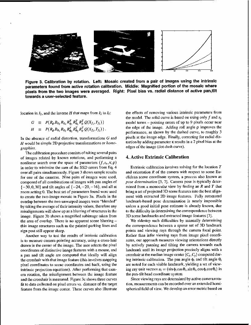
Figure 3. Calibration by rotation. Left: Mosaic created from a pair of images using the intrinsic parameters found from active rotation calibration. Middle: Magnified portion of the mosaic where pixels from the two images were averaged. Right: Pixel bias vs. radial distance of active pan,tilt towards a user-selected feature.

location in h, and the inverse H that maps from h to I\:

G = PiRpR^R^RlRlRlQiXf^Yf,))

H = PiRpR^R^R^R^RlQiXf^Yf,)).

In the absence of radial distortion, transformations G and H would be simple 2D projective transformations or tomo- graphies.

The calibration procedure consists of taking several pairs of images related by known rotations, and performing a nonlinear search over the space of parameters (f,sx,x,p) in order to minimize the sum of the SSD errors from Eq. 4 over all pairs simultaneously. Figure 3 shows sample results for one of the cameras. Nine pairs of images were used, composed of all combinations of images with pan angles of {-30,0,30} and tilt angles of {-24,-20,-16}, and all at zoom setting 0. The best set of parameters found were used to create the two-image mosaic in Figure 3a. Pixels in the overlap between the two unwarped images were "blended" by taking the average of their intensity values, therefore any misalignments will show up as a blurring of structures in the image. Figure 3b shows a magnified subimage taken from the area of overlap. There is no apparent scene blurring - thin image structures such as the painted parking lines and sign post still appear sharp.

Another way to test the results of intrinsic calibration is to measure camera pointing accuracy, using a cross-hair drawn in the center of the image. The user selects the pixel coordinates of distinctive image features with a mouse, and a pan and tilt angle are computed that ideally will align the crosshair with that image feature (this involves mapping pixel coordinates to scene coordinates and back, using the intrinsic projection equations). After performing that camera rotation, the misalignment between the image feature and the crosshair is measured. Figure 3c shows three curves fit to data collected on pixel errors vs. distance of the target feature from the image center. These curves also illustrate

the effects of removing various intrinsic parameters from the model. The solid curve is based on using only / and sx

model terms - pointing errors of up to 9 pixels occur near the edge of the image. Adding roll angle p improves the performance, as shown by the dashed curve, to roughly 3 pixels at the image edge. Finally, correcting for radial distortion by adding parameter K results in a 2 pixel bias at the edges of the image (dot-dash curve).

4. Active Extrinsic Calibration

Extrinsic calibration involves solving for the location T and orientation R of the camera with respect to some Eu- clidean scene coordinate system, a process also known as pose determination [3, 7]. Camera pose is typically determined from a monocular view by finding an R and T that bring a set of projected 3D scene features into the best alignment with extracted 2D image features. Fully automated landmark-based pose determination is nearly impossible unless a good initial pose estimate is already known, due to the difficulty in determining the correspondence between 3D scene landmarks and extracted image features [7].

We sidestep such difficulties by manually determining the correspondence between a sparse set of 3D landmark points and viewing rays through the camera focal point. Rather than infer viewing rays from image pixel coordinates, our approach measures viewing orientations directly by actively panning and tilting the camera towards each landmark until its image projection precisely aligns with a crosshair at the median image center (Cx, Cy) computed during intrinsic calibration. The pan angle <]),• and tilt angle 9, are noted for each visible landmark, yielding a set of viewing ray unit vectors «,• = (sin<|);Cos9j,sin0,-,cos<|>,cos9;) in the pan-tilt head coordinate system

Since viewing rays are determined by active camera rotation, measurements can be recorded over an extended hemispherical field of view. We develop an error metric based on

comparing the angle between pan-tilt viewing rays and direction vectors from the camera to 3D landmark points, and search for the pose that brings these two sets of unit vectors into best alignment.

First consider the case where we already know the camera location T (say by prior GPS measurement), and we only need to estimate its orientation R. Each 3D landmark sighting P{ yields two unit vectors, the viewing ray Uj as above, and a corresponding scene direction vector «,• = (Pi — T)/\\Pi - T\\ directed from the camera center T to the landmark point. If there were no noise in the measurements, these two vectors whould be related by camera orientation R as n, = Ru^ In actuality, the 3D landmark coordinates and the pan and tilt angles all contain measurement errors. Following Horn [5], we solve for the rotation R that best aligns these two sets of unit vectors («,-,«,-) in a least squares sense by maximizing

£ = £(".• •*«.•) = !( (Pj-T) \\Pi-T\\

Rut) (7)

Using an intermediate unit quaternion representation, the rotation R* that maximizes E can be computed in closed- form [5].

Now consider solving for full pose by maximizing (7) with respect to both T and R. As in earlier sections, we employ Powell's method. More specifically, we embed Horn's closed-form solution for R inside a Powell coordinate descent search on the three coordinates (Tx, Ty, Tz). For each tested value of T the closed-form solution for R is computed, and error function (7) is evaluated for that T and R. Experiments show that this hybrid Powell-Horn approach is remarkably insensitive to the initial estimate of T.

Experiments

A GPS survey was performed on five fixed-mount camera locations and two dozen landmark points located around the camera stations (see Figure 4). Measurements were taken with a Novatel RT-2 GPS receiver in communication with a similar Novatel base station located on site. These units provide dual carrier phase differential readings with roughly 2cm level accuracy.

For each camera, pan-tilt measurements were made of the landmark points visible to it, and the pose was computed using the hybrid Powell-Horn optimization procedure. Ac- curacy of the resulting pose estimate for each camera is summarized in the following table:

camera # landmarks dist err (m) ang err (deg) A 7 2.0 1.2 B 6 0.4 0.4 C 12 1.0 0.5 U 7 0.5 0.1 V 9 1.4 0.3

WfeSji rjftl mjj

vf 5gM Si i&L

Kg;

«pfc

WA ira Sk y|y£9ll

fclb? "rUfcw^^fc

Figure 4. Camera locations (white dots) and landmark locations (black) surveyed by GPS for pose estimation.

where distance error is the difference between the computed location and the location as measured by GPS, and angular error is the mean angle between corresponding unit vectors Hi and Rui.

The hybrid Powell-Horn pose estimation process is very stable when used with landmarks spanning a virtual hemi- sphere. T does not need to be initialized near the actual camera location, within the convex hull of the landmark points, or even close to the site, in order to converge to an accurate pose estimate. Figure 5 illustrates this behavior for one of the cameras. Seven landmark points were sighted, yielding a set of pan angles spanning a total range of 266 degrees, and a set of tilt angles spanning a range of 37 degrees. Initial estimates of T were generated every 200 meters on a 60X60 kilometer grid centered at the "ground-truth" camera location measured by GPS. For each initial position, camera pose was recovered using the Powell-Horn method, and the location component was compared to the ground-truth camera location. Each black grid cell represents an initial location from which the pose algorithm converged to within 2 meters of the ground-truth camera position. The entire set of landmark points is contained within a single grid cell in the center of the image (i.e. within a 200 X 200 meter area). The average radius of the convergence region is roughly 21 kilometers. Similar convergence properties were observed for the other cameras.

5. Applications and Future Work

We have developed a parameteric model for an active camera system with pan, tilt and zoom control. We have also incorporated active camera control into novel calibration methods for determining the intrinsic and extrinsic parameters of the model. This work was motivated by the

>

BK*.-. ■■aÄft&ä H&-

Hp W-äSgfl IHR**::, :i*liiH HKV

Kfra&- :'41isöHB

■vm f&wM

'^^pl HK&'-

' ; -ptf ■:?:'■?

Figure 5. Black pixels mark initial location estimates from which pose determination converged to within 2 meters of the ground-truth camera location measured by GPS.

need to calibrate in-situ a network of outdoor cameras for video surveillance applications. Accurate camera calibration was crucial to performing several image understanding tasks involved in video surveillance: actively tracking moving objects while rotating and zooming the camera, building image mosaics for operator visualization, pointing the cameras at known scene landmarks such as doorways, and estimating 3D object locations by intersecting viewing rays with a terrain model.

Further experiments are needed to compare the accuracy of flow-based intrinsic calibration methods to traditional methods using precise calibration grids in a controlled environment. The level of accuracy achieved is clearly good enough for performing outdoor surveillance tasks, but the limits on accuracy need to be established. In the current extrinsic calibration framework, each camera is calibrated separately, even though many cameras can see overlapping sets of scene landmarks. In future work we will perform simultaneous calibration of all sensors using a bundle ad- justment procedure to perform least-squares refinement of all sensor poses and landmark locations. Derivation of uncertainty bounds on computed pose is also future work.

Acknowledgements

We wish to thank our fellow VSAM team members: Alan Lipton, Dave Duggins, Hironobu Fujiyoshi, David Tolliver, Raju Patil and Yun-Ching Lee, for motivating this work and providing a cool working environment. Addi- tional thanks go to Dave Duggins for installing the cameras and performing the GPS survey of landmark positions, and to Takeo Kanade for his mentorship.

References

[1] A.Basu and K.Ravi, "Active Camera Calibration Us- ing Pan, Tilt And Roll," IEEE Trans SMC, Vol.B- 27(3), June 1997, pp. 559-566.

[2] J.Bergen et.al., "Hierarchical Model-Based Motion Estimation," ECCV, 1992, pp. 237-252.

[3] R.M.Haralick et.al, "Pose Estimation from Corre- sponding Point Data," IEEE Trans SMC, Vol. 19(6), Nov 1989, pp. 1426-1446.

[4] R.I.Hartley, "Self-Calibration from Multiple Views with a Rotating Camera," ECCV, 1994, pp.471-478.

[5] B.K.P.Horn, "Closed Form Solutions of Absolute Ori- entation Using Unit Quaternions," JOSA-A, Vol. 4(4), April 1987, pp. 629-642.

[6] TKanade et.al., "A Stereo Machine for Video-Rate Dense Depth Mapping and Its New Applications," CVPR, 1996, pp. 196-202.

[7] R.Kumar and A.R.Hanson, "Robust Methods for Es- timating Pose and a Sensitivity Analysis," CVG1P, Vol. 60(3), Nov. 1994, pp. 313-342.

[8] M.X.Li and J.M.Lavest, "Some Aspects of Zoom Lens Camera Calibration," IEEE Trans. PAMI, Vol. 18(11), November 1996, pp. 1110-1114

[9] W.H.Press et.al., Numerical Recipes in C, Cambridge Univ Press, New York, 2nd edition, 1992.

[10] G.P.Stein, "Accurate Internal Camera Calibration Us- ing Rotation, with Analysis of Sources of Error," ICCV, 1995,pp.230-236.

[11] D.Stevenson and M.M.Fleck, "Robot Aerobics: Four Easy Steps to a More Flexible Calibration," ICCV, 1995,pp.34-39.

[12] R.YTsai, "A Versatile Camera Calibration Technique for High-Accuracy 3D Machine Vision Metrology Us- ing Off-the-Shelf TV Cameras and Lenses," IEEE Journal of Robotics and Automation, Vol. RA-3, No. 4, August 1987, pp. 323-344.

[ 13] R.G.Willson, Modeling and Calibration of Automated Zoom Lenses, Ph.D. Thesis, Carnegie Mellon Univer- sity, CMU-RI-TR-94-03,1994.

[14] R.G.Willson and S.A.Shafer, "What is the Center of the Image?," JOSA-A, Vol.ll(ll), November 1994, pp. 2946-2955.

Using a DEM to Determine Geospatial Object Trajectories

Robert T. Collins, Yanghai Tsin, J. Ryan Miller and Alan J. Lipton The Robotics Institute, Carnegie Mellon University, Pittsburgh, PA. 15213

Email: {rcollins,ytsin,jmce,ajl}cs.cmu.edu

Abstract This paper addresses the estimation of moving ob-

ject trajectories within a geospatial coordinate system, using a network of video sensors. A high-resolution (0.5m grid spacing) digital elevation map (DEM) has been constructed using a helicopter-based laser range- finder. Object locations are estimated by intersecting viewing rays from a calibrated sensor platform with the DEM. Continuous object trajectories can then be assembled from sequences of single-frame location estimates using spatio-temporal filtering and domain knowledge.

1 Introduction Carnegie Mellon University and the Sarnoff Corpo-

ration are developing a Video Surveillance and Mon- itoring (VSAM) testbed that can seamlessly track human and vehicle targets through a large, visually complex environment. This apparent seamlessness is achieved using a network of active sensors to cooperatively track targets that cannot be viewed continuously by a single sensor alone. As targets move out of the active field-of-view of one sensor, they are "handed-off" to another sensor in the network. Au- tomated target hand-off requires representing the geometric relationships between: 1) multiple sensor locations and their potential fields-of-view, 2) target locations, velocities, and predicted paths, and 3) locations of scene features that may occlude sensor views or influence target motion (roads, doorways). In the VSAM testbed, this information is made explicit by representing all sensor pose information, target trajectories, and site models in a single geospatial coordinate system.

This paper addresses the issue of estimating geospatial target trajectories. In addition to their uses in planning sensor hand-off, such trajectories can be used to generate visual activity synopses for review by a human observer, to perform motion-based inferences about target behavior such as loitering, and to detect multi-agent interactions such as rendezvous or convoy- ing. In regions where multiple sensor viewpoints overlap, object trajectories can be determined very accurately by wide-baseline stereo triangulation. However, regions of the scene that can be simultaneously viewed by multiple sensors are likely to be a small percentage of the total area of regard in real outdoor surveillance applications, where it is desirable to maximize coverage of a large area given finite sensor resources.

Determining target trajectories from a single sensor requires domain constraints, in this case the assump-

tion that the object is in contact with the terrain. This contact location is estimated by passing a viewing ray through the bottom of the object in the image and intersecting it with the a digital elevation map (DEM) representing the terrain. Sequences of location estimates over time are then assembled into consistent object trajectories. Previous uses of the ray intersection technique for object localization have been restricted to small areas of planar terrain, where the relation between image pixels and terrain locations is a simple 2D homography [3, 4, 6]. This has the benefit that no camera calibration is required to determine the back- projection of an image point onto the scene plane, provided the mappings of at least 4 coplanar scene points are known beforehand. However, the VSAM testbed is designed for much larger scene areas that may contain significantly varied terrain.

The remainder of this paper discusses site modeling issues, emphasizing construction of a high-resolution DEM using a laser range-finder, the basic ray intersection technique for producing an estimate of object location from a single frame, and finally, techniques for producing consistent object trajectories from sequences of location estimates. Everything is illustrated using results from a VSAM testbed demonstration held in November 1997 at CMU's Bushy Run research facility.

2 Site Modeling The term "geo" spatial refers to coordinate systems

that represent locations on the surface of the Earth geoid - the ultimate absolute frame of reference for planetary activities. This does not necessarily im- ply a spherical coordinate system - local coordinate systems such as map projections can be geospatial if the transformation from local to geodetic coordinates is well documented. The primary benefit gained by firmly anchoring the VSAM testbed in geospatial coordinates is the ability to index into off-the-shelf cartographic modeling products. It is envisioned that future VSAM systems could be rapidly deployed to monitor trouble spots anywhere on the globe, with an initial site model being quickly generated from archived cartographic products or via aerial photogrammetry.

2.1 Coordinate Systems Two geospatial site coordinate systems are used in-

terchangeably within the VSAM testbed. The WGS84 geodetic coordinate system ("GPS" coordinates) provides a reference frame that is standard, unambiguous and global (in the true sense of the word). Unfor-

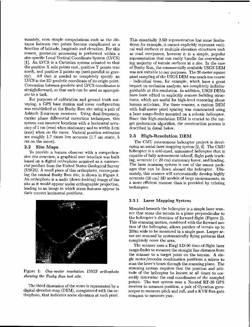
tunately, even simple computations such as the distance between two points become complicated as a function of latitude, longitude and elevation. For this reason, geometric processing is performed within a site-specific Local Vertical Coordinate System (LVCS) [1]. An LVCS is a Cartesian system oriented so that the positive X axis points east, positive Y points true north, and positive Z points up (anti-parallel to gravity). All that is needed to completely specify an LVCS is the 3D geodetic coordinate of its origin point. Conversion between geodetic and LVCS coordinates is straightforward, so that each can be used as appropriate to a task.

For purposes of calibration and ground truth surveying, a GPS base station and rover configuration was established at the Bushy Run site using a pair of Ashtech Z-surveyer receivers. Using dual-frequency, carrier phase differential correction techniques, this system can measure locations with a horizontal accuracy of 1 cm (rms) when stationary and to within 3 cm (rms) when on the move. Vertical position estimates are roughly 1.7 times less accurate (1.7 cm static, 5 cm on the move). 2.2 Site Maps

To provide a human observer with a comprehensive site overview, a graphical user interface was built based on a digital orthophoto acquired as a commercial product from the United States Geological Survey (USGS). A small piece of this orthophoto, encompass- ing the central Bushy Run site, is shown in Figure 1. An orthophoto is a nadir (down-looking) image of the site as it would appear under orthographic projection, leading to an image in which scene features appear in their correct horizontal positions.

Figure 1: One-meter resolution USGS orthophoto showing the Bushy Run test site.

The third dimension of the scene is represented by a digital elevation map (DEM), coregistered with the orthophoto, that indicates scene elevation at each pixel.

This essentially 2.5D representation has some limitations; for example, it cannot explicitly represent vertical wall surfaces or multiple elevation structures such as road overpasses, however it is a simple, popular representation that can easily handle the overwhelm- ing majority of terrain surfaces at a site. In the case of Bushy Run, the commercially available USGS DEM was not suitable to our purposes. The 30-meter square pixel sampling of the USGS DEM was much too coarse - individual trees, for example, which have a great impact on occlusion analysis, are completely indistin- guishable at this resolution. In addition, USGS DEMs have been edited to explicitly remove building structures, which are useful for high-level reasoning about human activities. For these reasons, a custom DEM with half-meter pixel spacing was constructed using a laser range-finder mounted on a robotic helicopter. Since this high-resolution DEM is crucial to the target geolocation algorithm, the construction process is described in detail below.

2.3 High-Resolution DEM The CMU autonomous helicopter project is devel-

oping an aerial laser mapping system [2, 9]. The CMU helicopter is a mid-sized, unmanned helicopter that is capable of fully autonomous takeoff, flight path tracking, accurate (< 20 cm) stationary hover, and landing. The laser scanning system is one of the sensor packages that can be flown aboard the helicopter. Ulti- mately, this scanner will automatically develop highly accurate (10 cm) 3D models of large environments, in a more efficient manner than is provided by existing techniques.

2.3.1 Laser Mapping System

Mounted beneath the helicopter is a simple laser scanner that scans the terrain in a plane perpendicular to the helicopter's direction of forward flight (Figure 2). This scanning motion, combined with the forward motion of the helicopter, allows patches of terrain up to 200m wide to be measured in a single pass. Larger areas are scanned by systematically flying patterns that completely cover the area.

The scanner uses a Riegl LD-90 time-of-flight laser range-finder to measure the straight line distance from the scanner to a target point on the terrain. A single motor/encoder combination positions a mirror to scan the laser's beam through the scanning plane. The scanning system requires that the position and attitude of the helicopter be known at all times to correctly determine the real coordinates of the sampled points. The test system uses a Novatel RT-20 GPS receiver to measure position, a pair of Gyration gyro- scopes to measure pitch and roll, and a KVH flux-gate compass to measure yaw.

Figure 2: Aerial mapping with a single planar scanner.

2.3.2 Bushy Run Mapping Procedure

The Bushy Run site was scanned to provide a high resolution DEM for object geolocation. The procedure for generating the DEM was as follows: 1) A GPS differential correction base station was setup at the Bushy Run site. 2) The helicopter mapping system was prepared for flight, and a local navigation frame was selected. 3) The helicopter mapping system was flown to scan the entire Bushy Run site. During the scan, the helicopter's position and attitude were collected and sent to ground computers for storage. Similarly, the laser scanner's measurements were also stored on the ground computers. 4) After the flights, the stored helicopter position and attitude were combined with the laser scanner's data to compute 3D coordinates of each point sampled by the laser range- finder. 5) The 3D data points were transformed from the helicopter's local navigation frame to the VSAM LVCS frame. 6) A DEM grid with cell size 0.5 m x 0.5 m was initialized. Each 3D point was assigned to one of the cells of the DEM by simply ignoring its Z component and allowing it to fall into one of the cells. For each cell of the DEM, three statistics were computed: the mean elevation of all points landing in that cell, the variance in the elevation of these points, and the total number of points. These three matrices comprise the resulting DEM.

2.3.3 Bushy Run Results

The Bushy Run site is approximately 300m x 300m, and has an asphalt road surrounding an open field with two large buildings and trees surrounding the area. A test pilot manually flew the helicopter about 10 meters above the road as the system scanned the surrounding environment. The flight was approximately 5 minutes in duration, and collected over 2.5 million 3D data points. Figure 3 shows a point cloud visualization of the data. For display purposes, each

point is shaded based on a combination of elevation, and on return intensity of the laser. As such, the road is readily visible. It should also be noted that since the helicopter was flown above the road, the low density of measurements from the center of the field is expected.

Figure 3: Perspective view of 3D point cloud from test scan.

Figure 4 shows a digital elevation map with 0.5m square grid spacing, generated from the scan data. The intensity of each pixel indicates the average elevation measured for that location. A side-by-side comparison of this image with the orthophoto in Fig- ure 1 indicates that the mapping system is producing reasonable results. For purposes of geolocation estimation, holes in the DEM (black areas in Figure 4) were filled be inserting bilinearly interpolated values from the USGS 30-meter DEM. This fusion of information was possible since both DEMS are precisely geolocated.

Figure 4: Half-meter resolution DEM showing same area as orthophoto in Figure 1. Intensity has been enhanced to emphasize terrain variation.

3 Estimating Target Location The VSAM testbed contains highly effective algo-

rithms for detecting, classifying and tracking moving targets through a 2D video sequence [7]. Target locations in the scene are estimated from the bounding box of stable motion regions in each frame of the sequence. Each location estimate is obtained by shooting a 3D viewing ray through the center of the bottom edge of the target image bounding box out into the scene, and determining where it intersects the terrain. This procedure is illustrated in Figure 5.

User view

Figure 5: Estimating object locations by intersecting view rays with a terrain model.

3.1 Camera Calibration Calibration of the internal (lens) and external

(pose) sensor parameters is necessary in order to determine how each pixel in the image relates to a viewing ray in the scene. The internal parameters of the sensor are determined manually, off-line. The external parameters consist of sensor location and orientation, measured with respect to the site LVCS. These are determined as part of the sensor setup procedure. Each sensor is mounted rigidly to a pan-tilt head, which in turn is mounted on a leveled tripod, thus fixing the roll and tilt angles of the pan-tilt-sensor assembly to be zero. The location (x0,y0,z0) of the sensor is determined by GPS survey.

The only other degree of pose freedom is the yaw angle (horizontal orientation) of the sensor assembly. This angle is estimated using a set of vertical landmarks distributed around the site, whose horizontal locations {x^yi) are known (surveyed by GPS). For each visible landmark the pan-tilt assembly is guided (by hand) to pan until the landmark is centered in the camera image, thereby measuring a set of pan angles {panî = l,...5n}. Each measured pan angle yields

an independent estimate Oi of camera yaw as

6i = atan2(?/i - y0,xt - x0) - pan^ .

A final yaw estimate 9 is computed as the average of these angles, taking care to use the appropriate for- mula for averaging angular data [8], namely

n n

6 = atan2(>^sin0*,V^cos0j) . l l

3.2 Ray Intersection with the DEM Given a calibrated sensor, and an image pixel corre-

sponding to the assumed contact point between an object and the terrain, a viewing ray (x0+ku, yo+kv, z0+ kw) is constructed, where (x0,yo,zo) is the 3D sensor location, (u, v, w) is a unit vector designating the direction of the viewing ray emanating from the sensor, and k > 0 is an arbitrary distance. General methods for determining where a viewing ray first intersects a 3D scene (for example, ray tracing) can be quite involved. However, when scene structure is stored as a DEM, a simple geometric traversal algorithm suggests itself, based on the well-known Bresenham algorithm for drawing digital line segments. Consider the vertical projection of the viewing ray onto the DEM grid (see Figure 6). Starting at the grid cell (x0,yo) containing the sensor, each cell (x, y) that the ray passes through is examined in turn, progressing outward, until the elevation stored in that DEM cell exceeds the z-component of the 3D viewing ray at that location. The z-component of the view ray at location (x, y) is computed as either

Z0 + (x - x0)

w or z0 + (y - yo) -w (1)

depending on which direction cosine, u or v, is larger. This approach to viewing ray intersection localizes objects to lie within the boundaries of a single DEM grid cell. A more precise sub-cell location estimate can then be obtained by interpolation. If multiple intersections with the terrain beyond the first first are required, this algorithm can be used to generate them in order of increasing distance from the sensor, out to some cut-off distance.

4 Assembling Target Trajectories Computation of dynamic object trajectories in the

scene is useful for planning sensor hand-off, generating visual activity summaries, and for performing qualitative behavior analysis. The previous section described how target locations can be estimated from each frame by intersecting viewing rays with a DEM. This section discusses the assembly of single-frame location estimates into continuous scene trajectories using spatio- temporal filtering and domain knowledge.

Figure 6: A Bresenham-like traversal algorithm determines which DEM cell contains the first intersection of a viewing ray and the terrain.

4.1 Spatio-Temporal Filtering Target trajectories can be created by simply con-

catenating a sequence of static object geolocations. However, some of these single-frame location estimates may be in error, due to imprecision in the motion region bounding box. Furthermore, a single viewing ray may intersect the terrain multiple times, and the first intersection is not always the correct one, since our "terrain" representation also contains trees and buildings that may occlude parts of the object. An example of this is shown in Figure 7a, corresponding to a video sequence in which a tracked vehicle became partially occluded by a tree. Composing single-frame estimates of the first intersection of the target viewing ray with the terrain generates a scene trajectory that incorrectly appears to swerve into the tree. Fig- ure 7b shows a better trajectory, generated by taking the last intersection between the viewing ray and the terrain. Although this simple heuristic is effective in removing errors caused by occluding foliage, it may yield incorrect results in rugged or hilly terrain, when multiple elevation structures such as bridges exist, or in the case of a person walking on a building roof.

A more general mechanism for assembling location estimates into smooth, continuous object trajectories is spatio-temporal filtering. For example, Kaiman filtering could be used to build a dynamic model of the target, based on the assumption that the target will not make sharp turns and abrupt accelerations [3, 6]. However, as mentioned above, a viewing ray may intersect the terrain multiple times, resulting in several alternative hypotheses for target location. The

Figure 7: Left: Unfiltered ray intersection trajectory shows a car "jumping" into a tree. Right: Filtered trajectory removes the treetop detour. Note that sensor locations and fields of view are also depicted on the user interface.

Kaiman filter, based on unimodal Gaussian densities, cannot simultaneously represent these multiple possible paths, and an incorrect choice of initial value will doom the entire trajectory. What is required is a more advanced filtering method that can handle multiple data associations, such as the CONDENSATION algorithm [5]. This is a topic of current work.

4.2 Domain Knowledge

Notwithstanding the need for a powerful, general mechanism to generate smooth target trajectories, in certain cases domain knowledge can be used to generate simpler, approximate solutions. In particular, the VSAM testbed classifies moving objects as being either human or vehicle [7]. Vehicular target motion is typically constrained to lie along roadways in the scene, and this heuristic suggests the use of a road network graph together with the viewing ray DEM intersection algorithm to produce unambiguous, accurate target trajectories.

For public roadways, the USGS digital line graph (DLG) product contains geolocated road networks as a connected graph of line segments. In the case of Bushy Run (private property), a road map was outlined by hand, using the digital orthophoto. Each vehicle location estimate was computed as a function of the target viewing ray, road network and DEM, as follows. As in Section 3.2, let the target viewing ray be written as (x0 + ku, 2/o + kv, z0 + kw). Both the viewing ray and road network curves are converted into 2D by vertical projection (ignoring their ^-components), and a set of intersection points (x,,t/j) between the viewing ray and road curves are computed, out to a cutoff distance. In general, the viewing ray will intersect the road map several times. Elevation information from the DEM is used to disambiguate between the multiple road location candidates, by choosing the the location (x, y) where the difference between DEM elevation and the

viewing ray z-component is smallest, that is

(x, y) = arg min lelevfo, yt) - rayz {xu yt) | ,

where the viewing ray z-component is computed as in Equation 1. This approach essentially finds the point with the minimum distance (measured vertically) between a 3D viewing ray and a set of space curves representing roads, but with low computational cost.

Figure 8 shows an activity synopsis generated using this approach, in the form of a long-term vehicle trajectory around the Bushy Run site. Two sensors cooperatively track a vehicle that drives into the site from the left, descends a hill into a parking lot, stops and turns around, then proceeds out of the parking lot and continues in its counterclockwise journey around the site. Gaps in the trajectory correspond to hand-off regions and occlusion areas where neither sensor was reliably tracking the object.

Figure 8: Activity synopsis of a vehicle driving through Bushy Run.

5 Current Work This year the VSAM IFD demo will be held in and

around the CMU campus, and feature nearly a dozen sensors tracking objects throughout a cluttered, urban environment. A full geospatial site model of the area is currently being constructed, including terrain, road networks, sidewalks, bridges, building volumes, and specific trees. The VSAM testbed will be able to manipulate these site model elements using libCTDB, a library of geometric utilities for interacting with a geospatial database, developed within the military's synthetic environments program. LibCTDB will support the VSAM testbed's need for occlusion analysis and ray intersection to support multi-sensor hand-off, as well as offer an interface to fully interactive, 3D dynamic visualization packages. Furthermore, more general methods of performing spatio-temporal filtering given multiple competing location hypotheses are being pursued.

Acknowledgements We wish to thank Omead Amidi and Marc De-

Louis for designing, building and operating the CMU Robot Helicopter, Daniel Morris for implementing the Bresenham-like ray intersection algorithm, and the cast and crew of the 1997 VSAM demo.

References [1] American Society of Photogrammetry, Manual of

Photogrammetry, Fourth Edition, American Soci- ety of Photogrammetry, Falls Church, VA, 1980.

[2] O.Amidi, T.Kanade and R.Miller, "Vision-based Autonomous Helicopter Research at Carnegie Mellon Robotics Institute," Proceedings of Heli Japan '98, Gifu, Japan, April 1998.

[3] K.Bradshaw, I.Reid and D.Murray, "The Ac- tive Recovery of 3D Motion Trajectories and Their Use in Prediction," IEEE PAMI, Vol.l9(3), March 1997, pp. 219-234.

[4] B.Flinchbaugh and T.Bannon, "Autonomous Scene Monitoring System", Proc. 10th Annual Joint Government-Industry Security Technology Symposium, American Defense Preparedness As- sociation, June 1994.

[5] M.Isard and A.Blake, "Contour Tracking by Stochastic Propagation of Conditional Density," Proc. ECCV, 1996, pp. 343-356.

[6] D.Koller, K.Daniilidis, and H.Nagel, "Model- Based Object Tracking in Monocular Image Se- quences of Road Traffic Scenes, IJCV, Vol.l0(3), June 1993, pp. 257-281.

[7] A.Lipton, H.Fujiyoshi, and R.Patil, "Moving Tar- get Identification and Tracking from Real-time Video," submitted to WACV 1998.

[8] K.V.Mardia, Statistics of Directional Data, Aca- demic Press, New York, 1972.

[9] R.Miller and O.Amidi, "3-D Site Mapping with the CMU Autonomous Helicopter," To appear in Proc. 5th Intl. Conf. on Intelligent Autonomous Systems, Sapporo, Japan, June 1998.

Fast Image-Based Tracking by Selective Pixel Integration

Frank Dellaert and Robert Collins Computer Science Department and Robotics Institute

Carnegie Mellon University Pittsburgh PA 15213

Abstract We provide a fast algorithm to perform image-based tracking, which relies on the selective integration of a small subset of pixels that contain a lot of information about the state variables to be estimated. The resulting dramatic decrease in the number of pixels to process results in a substantial speedup of the basic tracking algorithm. We have used this new method within a surveillance application, where it will enable new capabilities of the system, i.e. real-time, dynamic background subtraction from a panning and tilting camera.

1. Introduction/Philosophical Approach One of the fundamental tasks of real-time processing has been image-based tracking through a video sequence using a parametric motion model. This includes both tracking of a moving object through an image sequence [5] as well as registering of whole images to a reference view to provide software video stabilization [2,8].

Figure 1. Selective pixel integration selects pixels with a high information content with respect to the variables to be estimated. In this image, the pixels marked in white are informative with respect to pan, tilt and roll of the camera (click on the image to enlarge).

In this paper we will provide a fast algorithm to perform image-based tracking, based upon the following observation:

Using only a small percentage of the available pixels, selected on their information content with respect to the state variables, yields a tracking algorithm that is as accurate as conventional tracking algorithms that use entire images or image pyramids, yet orders of magnitude faster.

This observation relies on the fact that only very few pixels actually contribute towards the shaping of the error function that is minimized (see Figure 1). In the case of tracking, this is typically a weighted sum of square errors dependent on the parameters to be estimated. In the neighborhood of the minimum, the shape of the error function is governed by its Hessian. When inspected, the vast majority of pixels are seen to contribute little or nothing to the value of the Hessian, suggesting that these pixels can be safely ignored for the purpose of tracking.

Selective pixel integration is not yet another feature selection algorithm: we are truly selecting pixels, not small feature windows. Feature-based methods track the location of a small feature window, and the x-y coordinate of the feature is provided as input to the estimation method. In our case, we look directly at the value of a particular pixel. Each pixel will change in a predictable way as a function of the parameters, and thus each pixel in isolation provides some information on each of the parameters that cause it to change its value. The amount of information provided can be rigorously computed, as will be shown below. Based on this computed information content, we can designate some pixels as being better than others for estimating state variable updates.

2. Selective Pixel Integration 2.1 Definition and Example of Tracking

Template T Image I

h(X,T) x

V

waipedT = h(X/T)

X=[abcdefgh];

Figure 2. An example of a tracking problem is to estimate, over time, the parameters X=[a b c d efg h]' that warp the template T to the changing input image I, according to a 2D

projective transformation (a 2D homography).

We will define tracking as estimating the transformation between a reference image or template T and the current input image I over time. Let's define the state X and the measurement function h(X,T) that together specify this transformation. An example we will use throughout is the case where h is a projective warp of the template T, and X contains as components the eight independent parameters that are needed to specify the projective warp. The situation is illustrated in Figure 2.

The application we discuss below (as well as the example in Figure 2) involves whole images and is therefore more often referred to as image registration, but the algorithm we discuss is in no way limited to this type of application. Please refer to [6,5,4,3] for other examples of image based tracking, in particular face tracking, tracking of planar objects in 3D, and estimating lighting changes as well as deformations of shape. [5] also talks about how one can deal with outliers and occlusion, which we will not discuss in detail here.

2.2 A General Tracking Algorithm The most often used method to find an estimate for X at each time step is minimizing the sum of square errors:

X* = argmm(7- h(X,T)f (1) x

where we have used e2 as shorthand for e'e, and where ^'denotes the transpose of a matrix or vector e. This can be solved using the pseudo-inverse:

X* - X0 = (if' H)AH' (I-h(X,T)) (2)

where XQ is a prediction based on the previous tracking history, and H is the measurement Jacobian. It

is defined as the Jacobian matrix of h(.,.) with respect to X, and evaluated at XQ. If h is non-linear, more

than one iteration might be required to converge to the minimum.

2.2.1 The interpretation of the Measurement Jacobian

Figure 3. Jacobian images show how pixel values will change with respect to a change in state variables. An example image and its Jacobian images with respect to (in reading order) incremental camera roll, pan and tilt. Red and green are decrease and increase in pixel value, respectively. Intuitively, a change and pan and tilt will cause most change at vertical and horizontal edges, respectively. An equal amount of roll causes much less change in the image, with most change occurring at the edges and none in the middle of the image.

The measurement Jacobian has an intuitive explanation in terms of Jacobian images [4,3], which are a pictorial representation of how a pixel's value will change with respect to a change in state variables. They are simply the columns H- of the measurement Jacobian H, reordered as images. Hager [6,5] calls these images 'motion templates'. An example is shown in Figure 3.

It is clear that these Jacobian images, and thus H, are in general a function of the state X. Furthermore, they are expensive to compute, as each one of them is an image of the same size as the original template image. However, now there are n of them, where n is the dimension of X. Furthermore, they are in general non-linear and complex functions of the state and the template, as they are computed as the point-wise multiplication of induced flow fields and the template gradient images [3,5]. More about the computation of Jacobian images appears in the Appendix.

2.2.2 Computational Demands

The solution outlined above works, but is expensive, as hinted at in the previous paragraph. At each time step, and this possibly for multiple iterations, we need to compute (a) the Jacobian images H-, (b) the

pseudo-inverse (//' H)'1 H\ and (c) we need to warp the template T according to the changing estimate ofX.

One trick to reduce the computation is to warp the image I towards the template T instead, and minimize an approximate criterion:

dX* =argmin(A(X0-1,/)- h(dX,T)f (3)

dX

where h(X0A,I) informally denotes the inverse warp corresponding to h(XQ,T). We now look for the best

residual warp h(dX,T) that accounts for the difference between the warped image hiX^J) and the

template T. We then update the state estimate XQ using this incremental state update dX :

X*=X0®dX* (4)

with © denoting the update operation. The update might be a simple addition, as in the case of pure

translation, or matrix multiplication, when composing general projective transformations.

Again, using the pseudo-inverse, we get an expression for dX :

dX* = (#' H)A //' (h(X0-\l)-T) (5)

where our initial guess for dX is 0, i.e. we assume XQ is correct, and h(0,T)=T. This trick makes it

possible to pre-compute the Jacobian H, as we will always take 0 as the initial guess for dX, and so the Jacobian is evaluated only at 0. Thus, the pseudo-inverse of H can also be pre-computed [5].

2.2.3 Gaussian Pyramids

Although precomputing H saves a lot of computation, we still need to warp the image I at each time step, possibly multiple times if we need to iterate due to a non-linear h. Especially if I is large, e.g. complete images, this can be prohibitively expensive. One way to deal with this is to down-sample the images into a Gaussian pyramid. In many image registration applications enough accuracy can be obtained by only registering the low-resolution versions of I and T, and the cost of warping is not that high, as there are less pixels in the downsampled images. However, we still need to do the work of filtering and down-sampling to obtain the pyramid.

2.3 Selective Pixel Integration

A completely different approach is selective pixel integration, i.e. looking at the pixels in the original

images that yields the most information about dX. Intuitively, a pixel in a non-textured, flat area does not contribute much, if anything. Also, pixels that suffer from the aperture problem only contribute knowledge about part of the state. If we could find a small subset of the pixels that yield enough information about the state to satisfy our demands on accuracy, we could dramatically reduce the cost of warping, and thereby the overall cost of tracking, without downsampling.

It turns out that a similar question has been asked before in the MRI community [10]: suppose we can shoot any of thousands of rays at a person to get an MRI image reconstruction, but we want to use as few rays as possible, which ones should we choose ? In both cases, the underlying question is the same: Which measurements yield the most information about the quantity to be estimated ?

2.3.1 The'Best Pixel'

Suppose we could only look at one pixel, which pixel should we pick ? First, one pixel might yield only partial information about the state X. The answer will thus depend on what we already know. In addition, the matrix H'H in the pseudo-inverse will become singular in this case, as the measurement Jacobian H will be rank deficient. Both reasons prompt us to introduce prior knowledge.

\t& oh? ■ft.-«' Ts^-1

?■. v:rr?i!- d

Figure 4. The images above show the decrease in uncertainty resulting from looking atone pixel only. The actual quantity shown is the decrease in the trace of the state covariance matrix, relative to the prior information P. The brighter a pixel, the more information it provides. This heavily depends on our prior knowledge: at the left, the only uncertain state variable is the roll of the camera with respect to the template. In the image at the right, roll is known, but pan and tilt are not known precisely (up to one degree).

Let us assume that we can characterize our prior knowledge about dXby a Gaussian, centered around 0 and with covariance matrix P. We also need to know something about the measurement itself: how trustworthy is it? If we assume that the pixels are contaminated by i.i.d. zero-mean Gaussian noise, this information is specified by the variance <J . The maximum a posteriori or MAP estimate for dX, given one pixel j, is then found by minimizing a criterion which now takes into account the deviation of dX from 0:

dX* = argmin <r\fH(X^\ I) - hi(dX,T))2 + dX'P^dX (6)

where h- is the ith component of h, i.e. the recipe to warp one pixel according to X. This is done by

(repeatedly, if needed) solving the linear system of normal equations, with Hi the ith row of the Jacobian

H:

(a-2HlHi + F-^dX* = a~2Hl(h(X^J) - T) (?)

It is known from estimation theory that after convergence, the posterior distribution P(dX\I) (our full knowledge about dX) can be locally approximated as a Gaussian with covariance equal to the inverse of the Hessian Q:

P+ = («raÄjÄi + p-1)-1 = Q~l (8)

To find the best pixel, we would like to minimize this uncertainty. Although P+ is an n X n matrix

(where n is the dimension of the state X), the trace of P+ is also a meaningful quantity: it is equal to the expected variance of the error function after we obtained dX . Thus, one way to find the best pixel i is to minimize the trace of P+ [10]:

t = argmin Tr (a^HtHt + P~l)~l (9) t

Note that the identity of the best pixel is highly dependent on the prior knowledge P and on the form of h. In Figure 4, this is illustrated graphically for varying prior knowledge P. More examples of this dependence on P can be found here. Note also that all this can be generalized to arbitrary noise covariance matrices R, so that correlated noise can be modeled equally well.

2.3.2 The Best Subset of Pixels

Finding the best pixel is easy, but what about the best subset of pixels? It turns out this question is hard. Intuitively, the best pixel and the second best pixel do not necessarily constitute the best set of two pixels, as they might provide redundant information. In fact, the 'best pixel' might not even be a member of the best 2-set at all. in general, the only way the find the optimal set of M pixels, is to look at all possible subsets of size M within the m pixels. But this is a combinatorial search problem of immense proportions, as there are binomial(M m) such sets. With m on the order of 106 and M on the order 102, this is infeasible.

Figure 5. An example of selecting the subset of the best 1000 pixels in an image using the greedy SFS algorithm as described in Vite{Reeves95}. At the left, the set of 1000 pixels for known roll but unknown (incremental) pan and tilt. The color indicates the order in which pixels were selected by SFS, brighter meaning earlier in the sequence. As can be seen, mostly pixels on diagonal edges are picked out, as these provide information both on pan and on tilt. At the right, a set of 1000 pixels when pre-whitening is applied to remove spatial correlation.

A greedy algorithm was given in [10], based on a feature selection algorithm from machine learning, sequential forward search (SFS). In this algorithm, a list of pixels is created greedily. The procedure starts with a list containing only the best pixel, optimal in conjunction with the prior information P. The integration of this pixel gives a new covariance matrix, B, which now combines the information in P and the best pixel. Then, the best pixel is found that provides the most information relative to B. This process is repeated until M pixels are found.

We have implemented Reeves' SFS algorithm, and an example is shown in Figure 5. One problem that tends to arise, however, is that the selected pixels tend to cluster in the image, which would lead to non-robust tracking behavior in case of correlated noise such as occlusion, lens smudges etc... To remedy this, we have also applied pre-whitening to the Jacobian to cope with spatially correlated noise. The details are beyond the scope of this paper, but the effect is very noticeable. In the right panel of Figure 5, the new set of pixels obtained after pre-whitening is much more spread out, which is what we want.

2.3.3 Random Pixel Selection

For all the theoretical merit of Reeves' SFS algorithm, we have found that an even simpler algorithm provides more robustness in the case of image based tracking. Even the pre-whitened version of SFS still clusters pixels in a few regions of the image, which leads to instabilities in the tracking process in the case of occlusion. The answer we came up with is simple but works: we simply select M pixels randomly from the top 20 percent of the 'best' pixels. In other words, we compute an image like the one in Figure 4, sort the pixels according to information content (with respect to a prior), drop the bottom 80 percent, and randomly select M pixels from the remaining set. Examples of sets of pixels thus obtained are shown below in the application section.We have found that this simple method performs quite well in practice, and it is also straightforward to implement.

At the time of writing, we are also experimenting with an alternative method (also used by Zhang in a different context), that imposes an imaginary grid on the image, then select the M/N best pixels from each grid cell, where N is the number of grid cells. This forces the selections to be spread evenly over the whole image. For the selection within a cell, we again resort to Reeves' SFS. We are evaluating whether this method allows us to further reduce the overall number of pixels needed to accurately track.

2.3.4 The Selective Pixel Integration Tracker

The final tracking algorithm looks as follows:

1. Pre-compute the Jacobian images H for dX=0. 2. Pick a canonical prior knowledge covariance matrix P, and pixel noise covariance C . 3. Select the M best pixels for the template T, relative to P. 4. For each time step:

(a) Predict the state XQ using a model for the dynamics.

(b) Inverse warp the M selected pixels to the template,

(c) Calculate the error ei=Zi-T(mi),ie{l..M}

(d) Find the best dX* by solving (<TÎ^MHM + P-l)dX* = o^Hê

where HM is the part of H corresponding to the M selected pixels.

(e) Calculate X* = X0 © dX*

(f) Iterate if necessary

Most of the computation is now done off-line, and none of the on-line computation involves more than M pixels. The most expensive operations are the warp of the M pixels, and the computation of the Hessian Q = a~2Hf

MHM + P-1 • The latter can also be precomputed if it can be guaranteed that all

M pixels will be within the region to which I has been warped. If this is not the case, one can still save on computation by precomputing HM' HM, and subtracting the contribution for the relatively few pixels

that fall outside the valid set.

3. Discussion: Implications and Limitations The implications of our new method are potentially far-reaching. Since we can dramatically reduce the amount of computation spent on tracking, the CPU is freed to do other tasks that might otherwise have been impossible to do within real-time constraints. In the next section we will present the outline of this within a surveillance application.

In addition, we can increase the rate at which frames can be processed. Paradoxically, many tasks actually become easier to do at higher rates, e.g. frame or field rate, as the image displacements become smaller and easier to track over time, and we can use simpler motion models while still accurately

predicting what we should see in the next frame.

Finally, selective pixel integration provides an alternative to downsampling by working directly with the image pixels, and reasoning about what each individual pixel can tell us about the state variables.

It is also important to understand the limitations of this method. Most importantly, it will only work in a relatively small neighborhood around the true local minimum, as it depends crucially on the validity of the Jacobian H. Further away from the minimum, at best the algorithm will have to iterate multiple times, at worst it will diverge entirely. We feel, however, that this is not a significant limitation, as accurate predictions is always a hallmark of real-time applications: the better the prediction, the less computation needs to be expended.

There also a question of robustness: we have already remarked that the theoretically suporior method of Reeves' greedy selection scheme suffers from robustness problems when used with image based tracking. The random selection method works quite well in our example application (see below), but might integrate more pixel than strictly necessary. Indeed, in theory, 10 or 20 pixels should suffice to track, and we do indeed see that happen with synthetic sequences. More work is needed in the case of real images, though, to understand and model the noise and bring the number of pixels down even further.

4. Application: Real-Time Pan-tilt Tracking for VSAM

4.1 Motivation

The problem we address in this section is the detection of object motion from a continuously panning and tilting video camera. Over the past two years there has been a great deal of computer vision research devoted to automated video surveillance and monitoring (VSAM) [7]. A low-level task that is common to all video surveillance systems is to automatically detect moving objects (people and vehicles), and to track them as they move through the scene. Pan-tilt camera platforms can maximize the virtual field of view of a single camera without the loss of resolution that accompanies a wide-angle lens, and allows for active tracking of an object of interest through the scene.

Automatic detection of moving objects from a stationary video camera is easy, since simple methods such as adaptive background subtraction or frame differencing work well. These methods are not directly applicable to a camera that is panning and tilting since all image pixels are moving. However, this situation is approximately described as a pure camera rotation, and the apparent motion of pixels depends only on the camera motion, and not at all on the 3D structure of the scene. In this respect, the problem we are addressing is much easier than if the camera were mounted on a moving vehicle traveling through the scene.

At this time, adaptive background subtraction provides motion segmentation results with the least time lag and most complete object boundaries [11,9,13]. The general idea is to maintain statistics about the intensity or color values at each pixel in the image, and to gradually update these statistics over a moving window in time to adapt to lighting variations. Each new image is compared to this 'reference' image, and pixels that deviate significantly from their reference values are flagged as potentially

belonging to a new moving object. Object hypotheses are generated by performing connected components on the changed pixels, followed by blob tracking between video frames.

We ultimately seek to generalize the use of adaptive background subtraction to handle panning and tilting cameras, by representing a full spherical background model. There are two algorithmic tasks that need to be performed: 1) background subtraction: as the camera pans and tilts, different parts of the full spherical model are retrieved and subtracted to reveal the independently moving objects. 2) background updating: as the camera revisits various parts of the full field of view, the background intensity statistics in those areas must be updated.

Both tasks defined above, background subtraction and background updating, depend on knowing the precise pointing direction of the sensor, or in other words, the mapping between pixels in the current image and corresponding 'pixels' in the background model. Although we can read the current pan and tilt angles from encoders on the pan-tilt mechanism, this information is only reliable when the camera is stationary. Due to unpredictable communication delays, we can not precisely know the pan-tilt readings for a given image while the camera is moving. Our solution to this problem is to register the images to the current background model in order to infer the correct pan-tilt values while the camera is rotating.

4.2 Implementation

4.2.1 Scene Representation

Figure 6. The collection of views that we used in one experiment. There.are 40 views in total, with pan and tilt in the range 40:-20:100 and -4:-10:-44, respectively. The top-left image is the pan=40, tilt=-4 image. (Click on the image for a closer look)

Maintaining a background model larger than the camera's physical field of view entails representing the scene as a collection of images [8]. In our case, an initial background model is collected by methodically collecting a set of images with known pan-tilt settings. An example view set is shown in Figure 6. One approach to building a background model from these images would be to stitch them together into a spherical or cylindrical mosaic [8,12]. We choose instead to use the set of images directly, determining which is the appropriate one to use based on the distance in pan-tilt space. The warping transformation between the current image and a nearby reference image is therefore a simple planar projective transformation, rather than a more time consuming trigonometric mapping to the surface of a sphere or cylinder.

4.2.2 Pixel Selection

View ?: pan=-«01ill=-4, 250 selected

View38: pan=-SOiili=—*4, 250 selected

Figure 7. Two example views with the selected pixels. The state variables to be optimized are pan, tilt and roll.

For each of the views, the set of selected pixels for selective pixel integration is pre-computed, using the random selection algorithm outlined above. Two example sets are shown in Figure 7. The canonical prior we used had 1 degree standard deviation on pan and tilt, and 0.1 degrees on roll.

4.2.3 Tracking Pan and Tilt

Our tracking algorithm is described in detail below. For each time step, we:

1. Predict XQ, the pan, tilt and roll for the input image I, using a motion model (described in detail in

the next section).

2. Select the closest view T (in terms of pan and tilt)

3. Calculate the approximate homography ATj to warp T to I. Since we know the pan and tilt for the

view T, the calibration matrix K, and we have an estimate XQ for the pan, tilt and roll of the current

image, we can calculate this homography as A j = K Rj. Rj K where RT is the rotation matrix for the view T, and Rj is the estimated rotation matrix for the input

image.

4. Calculate the homography for the inverse warp, AlT = (ATj)~l

5. Inverse warp the M selected pixels to T, according to A7r For each of the selected pixels m-,

where % € {1..M}, we

(a) Calculate p{ = AlT m^ the corresponding image coordinate according to the projective warp

(b) If pi is not within the bounds of I, we discard this selected pixel.

(c) Resample the image I at that coordinate p{, obtaining gÂ!TJ), using either a bilinear or

Gaussian filter. Here g denotes the projective warp.

(d) Collect the resulting values in the measurement z Zi=gi(AÎ),i£{l..M}

(e) Collect the predicted values into the prediction y yi = T(mi)iie{l..M}

(f) Calculate the error erzry?

6. Optimize for the best incremental rotation dX* = [^ afy U>3]', by solving

(a-*H'MHM + P-1) dX* = a-*H'Me

where H is the pre-computed Jacobian with respect to incremental pan, tilt and roll (see Figure 3). The measurement function is a projective warp according to incremental pan, tilt and roll, parametrized using the incremental rotation matrix

1 -U)z <j)y

R(dX) = R(ux%ufy,uz) = ( uz 1 -u>x

-Wy U?x 1

7. Update the homography AlT and calculate X*. We can do this as

A%. <r- KR(dX*)K-lA!r

The final estimated rotation matrix for the image I is then obtained by RI = RTKl(AI

TylK

and X* = \pan tiltrolQ* can be easily calculated from Rr

8. Iterate if necessary

4.2.4 Multiple Model Prediction

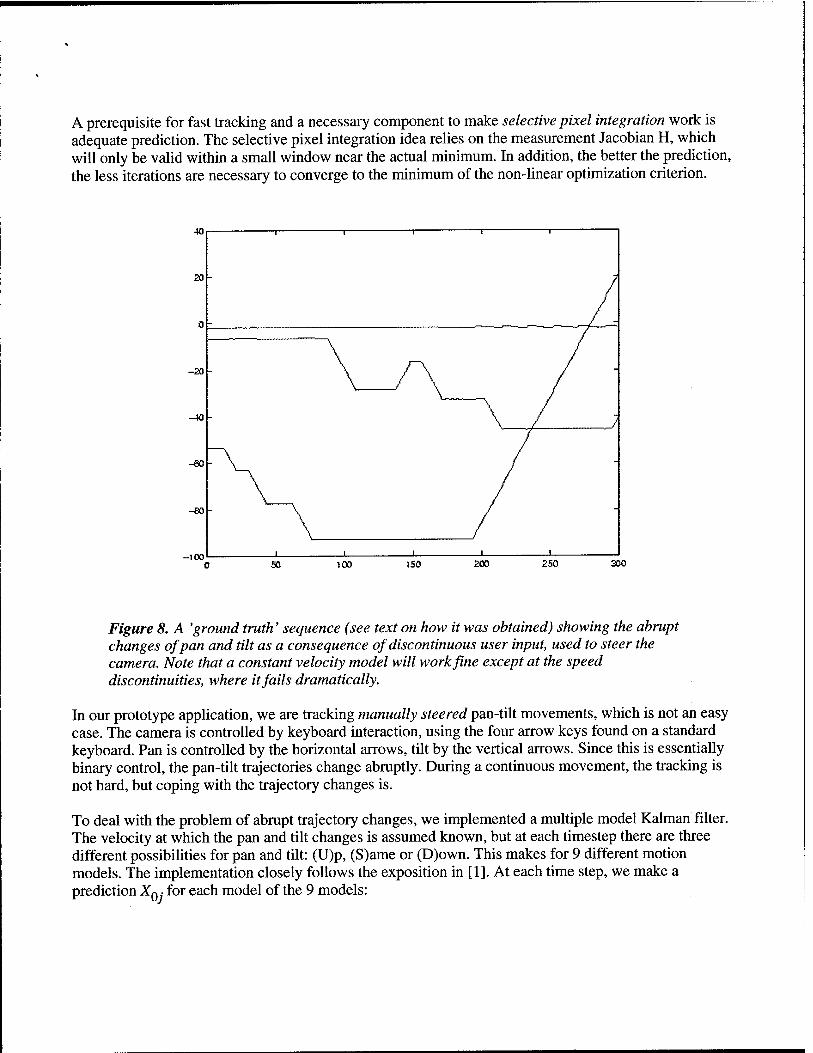
A prerequisite for fast tracking and a necessary component to make selective pixel integration work is adequate prediction. The selective pixel integration idea relies on the measurement Jacobian H, which will only be valid within a small window near the actual minimum. In addition, the better the prediction, the less iterations are necessary to converge to the minimum of the non-linear optimization criterion.

40

20

l 1 1 ■■■ ■

n

-20 \TV \ /

/

-» \ / \—f-— .7

-eo

"\

-

so

" \ i I i

so 100 ISO 200 2S0 300

Figure 8. A 'ground truth' sequence (see text on how it was obtained) showing the abrupt changes of pan and tilt as a consequence of discontinuous user input, used to steer the camera. Note that a constant velocity model will work fine except at the speed discontinuities, where it fails dramatically.

In our prototype application, we are tracking manually steered pan-tilt movements, which is not an easy case. The camera is controlled by keyboard interaction, using the four arrow keys found on a standard keyboard. Pan is controlled by the horizontal arrows, tilt by the vertical arrows. Since this is essentially binary control, the pan-tilt trajectories change abruptly. During a continuous movement, the tracking is not hard, but coping with the trajectory changes is.

To deal with the problem of abrupt trajectory changes, we implemented a multiple model Kaiman filter. The velocity at which the pan and tilt changes is assumed known, but at each timestep there are three different possibilities for pan and tilt: (U)p, (S)ame or (D)own. This makes for 9 different motion models. The implementation closely follows the exposition in [1]. At each time step, we make a prediction XQ ■ for each model of the 9 models:

Xo^xft-ij + n, (ii)

where Qj contains the hypothesized change in pan and tilt for model j. The likelihood of each model is

obtained by warping a severely subsampled version of the image (20 by 15 pixels, indicated by / and

Ts) to the hypothesized location in the template, and evaluating the sum of squared errors:

-1

The likelihood of model j given / is then (with ß a temperature parameter):

(12)

P(Is\j) = exp(-Q.5^) (13)

The posterior probability for each of the models is calculated based on the most likely model at the previous time step and a matrix of transition probabilities p... See [1] for additional details. After thi

y the model with the highest posterior probability is chosen for tracking.

4.3 Results

4.3.1 Evaluating Performance

(a) Camera Input (b) Selected View (c) Registered image (d) Difference Image

Figure 9. An embedded Quicktime movie showing a tracking sequence of 300 frames long (click here for downloadable MPEG, AVI, and higher resolution versions). The movie is divided in four panels: (a) The camera input shows what is seen by the camera during panning and tilting, (b) The selected view shows one of the (in this case) 40 input views to

which the current image is actively registered, (c) The registered image is the camera input after warping it to the selected view, (d) The difference image shows the difference between (b) and (c).

We have tested this algorithm based on several sequences of 300 frames in length, and consistently obtain tracking rates at about 60 frames per second, when integrating 250 pixels (M=250). This is with quarter size images, obtained by grabbing images from the camera and subsampling them by pure decimation.

To evaluate the performance of the algorithm, we do the frame-grabbing off-line, and store the images in memory. We store the images in memory because of two reasons: first, at the time of writing we only have a prototype system working, which is not yet integrated with our on-line frame-grabbing software. We do not believe the overhead of image and memory I/O will significantly impact the timing results. Second, we our method performs at much higher than frame rates, and when grabbing at a fixed framerate we would have no way to assess the algorithm's performance.

We then run the tracker, and note how long it takes to process all 300 frames. This is always around 5 seconds, with fluctuations because the number of iterations per frame might differ from frame to frame. We are convinced that these preliminary performance figures can yet be improved upon, as part of our research code still runs within MATLAB. We are currently porting the entire algorithm to C++.

-to

2D

-20

-W -

-GO -

-BO -

-100

1 1 1 1 1

-

"■.

\ / ■>

\ ■' ~

- pan

lili t-

i i i i i

50 100 150 200 250 300

Figure 10. Estimated pan, tilt and roll.

1

OB

OB

0.4

02

0

ri'T 1 i 1— 1

' • i t 'i :! '{ ' 1 » j ► «! - ' i ü !

1 1 i i . - 1

D 1 - - S i

l: -

_ i: 1 i i . .

' 1 1 ' ' 50 100 ISO 200 250 300

1 i 1 i

!.'• .., i

OB f i

) 1 i j 1 ! f

3

5

OB 1 1

i j j

1 1 i i i i

; i ! i i

i

1 i j i i \

j

i

i

f t

i f

0.4

02

D S

0 L u ;l « 1 :, i

'■I _t___. 1 1 1 1 1

50 100 150 200

T

250

L

300

Figure 11. Marginal posterior probabilities for the different motion models. The top panel shows the posterior probability of three different models for pan: (U)p, (S)ame, and (D)own. The bottom panel

shows the same for tilt. Note the correspondence with Figure 10.

A video segment recording the tracking of a typical sequence is shown in Figure 9. The measured pan, tilt and roll angles are shown in Figure 10. The posterior probability of each motion model is shown in Figure 11.

4.3.2 Evaluating Tracking Accuracy

Ob ■ I 1 l i

0.4

s :|

i i

ii [

-

02 } i 'l- - '•;1

ii ■ -. t l!; -

0 i-~

— - /•'■• ■•if ii

-fC'r-

i S

'i1*'" •c * "H l! ii ' -';• :' :■

-02 f !

1 1 I

: =:;; :; i "

-0.4 ■:;

; j -

-OS - : -

-OS - -

-1 ) i i i

-12 pan UK

i ■ ( ■ 1 50 100 ISO 200 250 300

Figure 12. Comparison with ground truth.

To evaluate the accuracy of the algorithm, we obtained 'ground truth' by running the tracker using 3-level pyramids of the images and the views, and using all pixels. Because of the hierarchical approach, the initial estimates at higher-resolution levels are very good and high accuracy is obtained. Since we use complete images up to a quarter size, this approach is slow but yields accurate results. The comparison of the estimated pan-tilt-roll angles with the ground truth is shown in Figure 12. Most of the noticeable spikes are associated with shifts between views.

5. Conclusion We have presented a novel approach to obtaining better-than-frame-rate image-based tracking. It relies on the selective integration of a small subset of pixels that contain a lot of information about the state variables to be estimated. This dramatic decrease in the number of pixels to process results in a substantial speedup of the basic tracking algorithm. We have used this new method within a surveillance application, where it will enable new capabilities of the system, i.e. real-time, dynamic background subtraction from a panning and tilting camera.

Appendix: Computing the Jacobian Images

The calculation of the Jacobian images is detailed by Dellaert [4]. Hager & Belhumeur have a similar derivation in [6,5]. Our paper [4] is available on-line:

Jacobian Images of Super-Resolved Texture Maps for Model-Based Motion Estimation and Tracking F. Dellaert, S. Thrun, and C. Thorpe, IEEE Workshop on Applications of Computer Vision (WACV'98), Princeton, New Jersey, October 19-21, 1998, pp. 2-7. Download: pdf [262 KB], ps.gz [798 KB] copyrighted

In essence, the calculation amounts to a simple application of the chain rule: the Jacobian H at XQ is

defined as the partial derivative of h with respect to X, evaluated at X0:

H{XQ)=wm dx (14)

Xo

which is a m X n matrix, with m is the number of pixels in an image, and n the dimension of the state.

One entry J7~ is the partial derivative of pixel hfX,T) with respect to state variable X •:

IT (Y \ — dhi{X}T) •"tflAoJ - —^ dXi x*

(15)

If/?(.,.) is a warp implemented by simple point sampling, h has the form hfXJ) = 7(/(p;,X),r), where f

is the coordinate transform that transforms image coordinate p- accoring to X into an template

coordinate m-fip^X). It is a 2 X 1 vector valued function. Substituting this in equation (15) and

application of the chain rule gives:

HV(XQ) - dfrfo^H dXi x0

= ar(/fa*)) dXi

dT

PiiXf, dm a/fa x)

m dXi (16)

Pi>Xo

where Jj£ is the 1 by 2 gradient vector of T, evaluated at m., and g^%ffi

flow vector induced a change in X-, evaluated at pi and XQ.

is the 2 by 1 pi,Xo

Example

A graphical example is given below for a circular patch, texture mapped with a checkerboard pattern,

and moving in 3D. The state variables involved are yaw,pitch,roll and 3D translation:

, wKits, ' >.. ' ■'

'■m- ' ■..%»■- - .,,., ^......

The original texture mapped image, and its associated template gradient images.

— - \

!! ii^

* ■> -.

■ w- ■*«* *» > ^\ \.. * * *

' ■> \ - -.

11 - »V-

Induced flow fields for all state variables. From left to right: X, Y, Z, yaw, pitch, and roll.

A

The six resulting Jacobian images. From left to right: X, Y, Z, yaw, pitch, and roll.

Bibliography

1 Y. Bar-Shalom and X. Li. Estimation and Tracking: principles, techniques and software. Yaakov Bar-Shalom (YBS), Storrs, CT, 1998.

2 J. R Bergen, P Anandan, Keith J Hanna, and Rajesh Hingorani. Hierarchical model-based motion estimation. In G Sandini, editor, Eur. Conf. on Computer Vision (ECCV). Springer-Verlag, 1992.

3 Frank Dellaert, Chuck Thorpe, and Sebastian Thrun. Super-resolved tracking of planar surface patches. In IEEE/RSJ Intl. Conf. on Intelligent Robots and Systems (IROS), 1998.

4 Frank Dellaert, Sebastian Thrun, and Chuck Thorpe. Jacobian images of super-resolved texture maps for model-based motion estimation and tracking. In IEEE Workshop on Applications of Computer Vision (WACV), 1998.

5 G. Hager and P. Belhumeur. Efficient regions tracking with parametric models of geometry and illumination. IEEE Trans, on Pattern Analysis and Machine Intelligence, October 1998.

6 G.D. Hager and P.N. Belhumeur. Real time tracking of image regions with changes in geometry and illumination. In IEEE Conf. on Computer Vision and Pattern Recognition (CVPR), pages 403-410, 1996.

7 T. Kanade, R. Collins, A. Lipton, P. Burt, and L. Wixson. Advances in cooperative multi-sensor video surveillance. In DARPA Image Understanding Workshop (IUW), pages 3-24, 1998.

8 R. Kumar, P. Anandan, M. Irani, J. Bergen, and K. Hanna. Representation of scenes from collections of images. In Representation of Visual Scenes, 1995.

9 A. Lipton, H. Fujiyosh, and R. Patil. Moving target classification and tracking from real time video. In IEEE Workshop on Applications of Computer Vision (WACV), pages 8-14, 1998.

10 S. J. Reeves. Selection of observations in magnetic resonance spectroscopic imaging. In Intl. Conf. on Image Processing (ICIP), 1995.

11 P. Rosin and T. Ellis. Image difference threshold strategies and shadow detection. In British Machine Vision Conference (BMVC), pages 347-356, 1995.

12 H.-Y. Shum and R. Szeliski.

Construction and refinement of panoramic mosaics with global and local alignment. In Intl. Conf. on Computer Vision (ICCV), pages 953-958, Bombay, January 1998.

13 C. Stauffer and W.E.L. Grimson. Adaptive background mixture models for real-time tracking. In IEEE Conf. on Computer Vision and Pattern Recognition (CVPR), volume 2, pages 246-252, 1999.

About this document... Fast Image-Based Tracking by Selective Pixel Integration

This document was generated using the LaTeX2HTML translator Version 98.1pl release (March 2nd, 1998)

Copyright © 1993, 1994, 1995, 1996, 1997, Nikos Drakos, Computer Based Learning Unit, University of Leeds.

The command line arguments were: latex2htnil-split 0 -show_section_numbers -local_icons -no_navigation framerate.tex.

The translation was initiated by on 1999-08-26

1999-08-26

Local Application of Optic Flow to Analyse Rigid versus Non-Rigid Motion

Alan J. Lipton The Robotics Institute, Carnegie Mellon University, 5000 Forbes Ave, Pittsburgh, PA, 15213

email: [email protected], URL: http://www.cs.cmu.edur vsam

Abstract

Optic flow has been a research topic of interest for many years. It has, until recently, been largely inapplicable to real-time video applications due to its computationally expensive nature. This paper presents a new, reliable flow technique called dynamic region matching, based on the work of Anandan[l], Lucas and Kanade[10] and Okutomi and Kanade[ll], which can be combined with a motion detection algorithm (from stationary or stabilised camera image streams) to allow flow-based analyses of moving entities in real-time. If flow vectors need only be calculated for "moving" pixels, then the computation time is greatly reduced, making it applicable to real-time implementation on modest computational platforms (such as standard Pentium II based PCs).

Applying this flow technique to moving entities provides some straightforward primitives for analysing the motion of those objects. Specifically, in this paper, methods are presented for: analysing rigidity and cyclic motion using residual flow; and determining self-occlusion and disambiguating multiple, mutually occluding entities using pixel contention.

Keywords: optic flow, motion analysis, tracking

1 Introduction

Analysing the motion of entities in a video stream is an important, current research challenge. Groups such as the entertainment industry use motion captured from video imagery to generate computer graphic characters and avatars for movies, computer games, and web-based applications. These motion capture techniques usually require a large investment of operator time and effort. As applications become more interactive, it will be increasingly important to automate the analysis of moving objects in real time. In applications such as automated video surveillance[7], it is essential to be able to understand the different motions of objects and infer their behaviours - such as the difference between two joggers meeting in a park, and a mugging.

Presented in this paper is a new strategy for divining some low-level motion parameters in real-time from entities in video streams. A new optic flow technique called dynamic region matching is applied locally to blobs extracted using an adaptive background subtraction motion detection algorithm[4]. Computing flow only for "moving" pixels allows real-time implementation on even modest compu-

tational platforms (such as Pentium II PCs). The resulting local flow fields can be used to analyse the motions of those blobs. Specifically, this technique is used to determine rigidity of motion, determine self-occlusion, and disambiguate mutually occluding moving objects.

1.1 Optic Flow

Optic flow techniques are traditionally used to determine camera motion or reconstruct 3D scene structure. In these cases, only the gross flow of large scene components is required and real-time performance is not necessary. Conse- quently, most flow techniques provide sparse results over an entire image or are extremely computationally expensive. Furthermore, most algorithms fail in largely homogeneous regions (ie. regions lacking texture). Although Anandanfl] provides a measure for determining just how bad a flow vector is, most algorithms make no effort to improve flow vectors in homogeneous regions.

Barron, Fleet, and Beauchemin[2] divide flow techniques into four categories: differential methods; region- based matching; energy-based; and phase-based. Of these, the most amenable to real-time implementation are the differential methods and the region-based matching methods. The differential methods such as Lucas and Kanade[10] effectively track intensity gradients in the scene. The advantage of this is that reliable flow vectors can be determined based on the information (measured by intensity gradient) content of a scene. However, one of the assumptions behind this method is that there is no deformation in the objects in the scene. Clearly an unreasonable assumption when determining the motion of a entity like a human being. Region- based matching techniques such as Anandanfl] track small regions in the scene from frame to frame. These methods are more robust to deformable objects, but are susceptible to large errors where there is little texture in the scene.

1.2 Motion Analysis

The ultimate goal of motion analysis is to describe activities occurring in video streams. Primitive analyses have concentrated on simply determining the rigidity of moving objects as a precursor to more complex recognition schemes[13]. Others go further and attempt to fit models (2D or 3D) to objects[5, 8] in order to analyse their motions. More complex schemes attempt to interpret and char- acterise particular motions[4, 3] such as walking, running, sitting, doing push-ups, etc.

With reliable flow vectors for every pixel in a blob it becomes possible to track individual pixels from frame to frame. This capability can be employed to cluster pixels into "body parts" for model-based motion analyses (such as pfinder[14] and W4[5]). It also means that an object's rigidity can be determined by calculating residual flow - that is the motion of "body parts" relative to the blob's gross motion. It is clear that a human or animal will have limbs moving relative to each other and to the gross body motion whereas a vehicle will not. By clustering residual flow vectors, it is even possible to extract these "body parts". Fi- nally, a property called pixel contention is introduced in this paper to analyse occlusion. When flow is computed for an object that is occluded either through self-occlusion (such as an arm swinging in front of the body) or by another body (such as a person walking behind something else), some of the pixels will "disappear" from one frame to the next causing competition between pixels or invalid flow vectors. This pixel contention can be measured and used to determine when such occlusions are occurring.

Section 2 of this paper describes blob detection and tracking. Section 3 describes the new dynamic region matching algorithm for computing a dense flow field within the pixels of a moving entity. Section 4 describes how residual flow can be used to determine the rigidity of a moving object. Section 5 describes the pixel contention measure of occlusion and explains how it can be applied to determine self-occlusion within an object or mutual occlusion between two objects.

2 Detection and TYacking of Moving Blobs

/ ' i \ \ \

/ / I \ \ \

A Figure 1. Moving blobs are extracted from a video image.

Detection of blobs in a video stream is performed by the method described in [4]. This is basically a process of background subtraction using a dynamically updating background model.

Firstly, each frame is smoothed with a 3 x 3 Gaussian filter to remove video noise. The background model Bn (x)

is initialised by setting B0 = I0. After this, for each frame, a binary motion mask image Mn (x) is generated containing all moving pixels

Mn(a (I: \In(x)-Bn_1{x)\>T \In(x)-Bn^(x)\<T (1)

Where T is an appropriate threshold. After this, non- moving pixels are updated using an IIR filter to reflect changes in the scene (such as illumination)

"»W-\ alnW + il-^B^x), Mn{x) = 1 Mn{x) = 0

(2) where a is the filter's time constant parameter. "Mov- ing" pixels are aggregated using a connected component approach so that individual blobs can be extracted. An example of these extracted blobs is shown in figure 1.

Tracking a blob from frame to frame is done by the template matching method described in [9]. The important feature of this tracker is that, unlike traditional template tracking which has a tendency to "drift" when the background becomes highly textured, this method only matches pixels which have been identified as "moving" by the motion detection stage - thus making it more robust.

2.1 Tracking Through Occlusion

When two objects being tracked are predicted to occlude

(XBO + VßoSt) f« (XBI + VßlSt) (3)

(where XBO, VBO, #BI and VB\ are the positions and velocities of the two objects respectively, and 6t is the time between consecutive frames) it becomes hard to track them using the template matching algorithm of [9], not because the template matching fails, but because it becomes difficult to update a template as it will be corrupted by pixels from the other object. In fact, when two blobs are close to occluding, the motion detection algorithm will detect them as only a single blob\

The problem can be addressed by storing the previous views of each object over time. When an occlusion is about to occur, synthetic templates can be generated to use in the template matching process. If the object is determined to be rigid by the method of section 4, then the latest view is used as a synthetic template while the occlusion is occurring. On the other hand, if the object is determined to be non-rigid, then its periodicity is determined by a process akin to Selinger and Wixson[13]. The latest view is matched with the previous views to find the best synthetic template. Then, as the occlusion continues, new synthetic templates are generated by stepping through the list of previous views.

Synthetic templates

Figure 2. Two examples of tracking through occlusion. The blobs are tracked using synthetic templates derived from previous views

An example of this procedure is shown in figure 3. While the occlusion lasts, blobs from previous views of the object are substituted for the potentially corrupted data. These synthetic blobs are used for matching until the occlusion is over.

Figure 2 shows two examples of tracking through occlusion. In both cases synthetic templates are derived from previous views of both blobs and thus they can be disambiguated even when they are in the process of occluding. Pixels tinted red belong to the occluding object, and pixels tinted blue belong to the occluded object.

3 Optic Flow by Dynamic Region Matching

To analyse the motion of a character in a video stream it is necessary to acquire a dense, accurate flow field over that object, perhaps even a flow vector at every pixel. To obtain a legitimate flow vector for every pixel in an area, region- based matching is the obvious choice. But to make sure the flow vectors are realistic, it is necessary to have enough texture in the region to ensure a good match. This can be achieved by using a dynamic region size similar to the approach of Okutomi and Kanade[12]. The idea is to use edge gradients as a measure of information and, at every pixel position, grow the support region until there is enough edge gradient information to justify matching. Furthermore, flow needs to be computed only for pixels contained within the moving object. Consequently, this particular implementation is only valid for video streams derived from stationary cameras, or streams which have been stabilised.

3.1 The Region Matching Algorithm

Consider a stabilised video stream or a stationary video camera viewing a scene. The returned image stream is denoted In (x) where J is a pixel intensity value, n is the frame number and x represents a pixel position in the image (i, j).

If images in the stream are St (time) apart, then a particular pixel in the image will move by a distance v(x)8t where v(x) = (vi(x), Vj(x)) is the 2D image velocity ofthat pixel. This can be found by matching a region in /„ to it's equivalent region in In+i by minimising a distance function D(x; d) where d represents a linear translation (rf,, dj).

Firstly, a region W(x)In(x) is defined by multiplying Jn

with a 2D windowing function W(x) of size (W,-, Wj) centered on pixel x. This region is then convolved with the next image in the stream In+\ to produce a correlation surface D(x; d). The range of values over which the convolution is performed d 6 [do, di] must be specified.

i=WiJ=Wj

D(x;d)= £ £ \W(i,j)In(i,j)-In+i((i,j) + d)\

\\W(x)\\

(4) where | [W(a;)|| is a normalisation constant given by

i=W, j=Wj

iiw(*)ii= E E w&j) »•=i j=i

(5)

Figure 4 shows a typical correlation surface for a region match. The minimum of D(x;d) is then computed to sub-pixel accuracy by approximating the surface with a quadratic function D{x; d).

The true pixel displacement dmjn is taken as the minimum of the approximate surface

rfmin = minD(x;d) (= v(x)St) (6) d

3.2 Computing Local Flow

Having established a track between a blob fi„ in In and a blob fi„+i in 7n+i and the gross velocity VB (from the tracker) between them, it is possible to determine the flow of every "moving" pixel. The idea is to take a small region around each pixel in fin and match it with its equivalent

mit Hill I iHDl

Negative Correlation Surface [-D(x;d)]

Current view

Hill III

Frame Number

Figure 3. Template matching the current view of a blob with previous views allows a synthetic template to be used when it is occluded.

Figure 4. A typical correlation surface (inverted for easier viewing)

"Vertical" Information "Horizontai"Vnformaffon

Adequate Adequate

region in fi„+i. The method used is similar to Anandan'sfl] method with several distinctions. Anandan uses a pyramid to perform matching. In this implementation, a pyramid is unnecessary as the number of pixels for which flow is computed is not large. In Anandan's work, the Laplacian of the image is used. This provides a confidence measure for each flow vector. If there is not enough information in a region, the confidence on the flow vector is low. In this implementation, the image itself is used and confidence is measured using the content of the region. Anandan uses fixed 3x3 regions for matching. Here, as in Okutomi and Kanade[ll], the regions are dynamic and are grown until there is enough information to ensure a reliable match.

The flow computation per pixel is a two-pass process. Firstly, an appropriate support region is found to ensure that enough information is present to obtain a valid flow vector. And then a region matching is performed to compute the flow vector.

3.2.1 Computing the Support Region

To ensure a good match between regions, it is essential that enough information is available in both horizontal and vertical directions around the central pixel a;. So a support region

Figure 5. Growing the region around a pixel to ensure adequate information content in both vertical and horizontal directions.

around x is iteratively grown and the enclosed information content is measured until it reaches a predetermined threshold Tj. To measure horizontal and vertical information, a Sobel filter is used. Prior to the matching process, two images SH(X) and Sv{x) are computed from /„ by filtering using the standard Sobel operators.

SH{x) -

Sv(x) =

' 1 0 -1 1 2 0 -2 4

1 0 -1 1 2 1 0 0 0

-1 -2 -1

*In(x)

In(x)

(7)

Starting with a 3 x 3 support window W(x) centered on x two information measures are calculated: vertical image information Ev; and horizontal image information EH

% = EE^^(i'.i) (8)

£v = EE^j)^(^') (9) ' 3

The algorithm for determining the ultimate window size is as follows

Do Calculate EJJ by equation 8 Calculate Ey by equation 9 HEH <Tj

Increase Wi by 2 pixels If£V <Ti

Increase Wj by 2 pixels Until both EH and Ev are > 7}

Figure 5 shows a graphical representation of how the algorithm is applied to select an appropriate support region around a pixel.

3.2.2 Computing the Flow Vector

Motion of individual pixels can be modeled as as the gross motion of the blob VB plus some residual pixel motion VR{X). Thus

v(x) = vB + VR(X) (10)

If it is assumed that the residual motion of pixels within Cin is not very great, then the correlation surface D(x; d) to compute the flow vector for a given pixel x need only be evaluated over a small range around d = VßSt.

Using the 2D windowing function W(x) as determined by the algorithm of section 3.2.1, the flow v(x) for pixel x can be computed using the method of section 3.1. One limitation of this method is that background texture can corrupt the flow vector calculation. To ameliorate this, the elements of W(x) can be weighted to give preference to "moving" pixels (expressed as a binary image Mn), for example

W'(x) = W{x){l + Mn{x)) (11)

Anandan[l] uses the curvature of the correlation surface around the minimum as a measure of confidence in the flow vector. This is a reasonable choice if the information content of the region is unknown. Homogeneous regions will be characterised by correlation surfaces with high radii of curvature (infinite in the ultimate case). However, in this implementation, the information content is known, so a simpler metric for confidence is used. Here, the value of the correlation surface's minimum Dmm (x; d) is taken as a confidence measure. Regions which match well will have low values of Dm\n(x; d) whereas regions which do not match well will have higher values. This property can be used in outlier rejection and to calculate pixel contention as in section 5. Figure 6 shows the flow fields and confidence measures for two different blobs.

4 Rigidity Analysis by Residual Flow

Given the gross motion of the moving body VB as calculated in section 2, and the flow field v(x) for all of the pixels in that body, it is possible to determine the velocity of the pixels relative to the body's motion VR(X) by simply subtracting off the gross motion

VR(X) vB (12)

to find the residual flow. It is expected that rigid objects would present little resid-

ual flow whereas a non-rigid body such as a human being would present more independent motion. When the average absolute residual flow per pixel

VR = EiLi VR(X

) X

(13)

(where X is the number of pixels in the blob) is calculated, it not only provides a clue to the rigidity of the object's motion, but also its periodicity. Rigid objects such as vehicles display extremely low values of VR whereas moving objects such as humans display significantly more residual flow that even displays a periodic component.

Figure 7(a) shows the residual flow from two objects. Clearly, there is a large amount of independent pixel motion in the case of the human, and there is almost none in the case of the vehicle. A simple clustering based on his- togramming the residual flow vectors clearly shows group- ings of these flow vectors and could facilitate the extraction of "body parts" such as arms and legs. Figure 7(b) shows how residual flow can be used a measure of rigidity for humans and vehicles.

5 Occlusion Analysis by Pixel Contention

Many researchers have noted problems with tracking objects or their component parts through occlusions. One of the big selling points of the Condensation algorithm of Isard and Blake[6] is that it successfully tracks objects' shapes through deformations and occlusions. The patterns of optic flow can also be used as a key to object occlusions, whether they be caused by self-occlusion, or occlusion with other bodies. A pixel contention metric can be used to detect when occlusion is occuring, and even extract the spatial ordering. The object in front will display less pixel contention than the object in the rear.

When occlusions happen in the 3D world, they appear as 2D deformations. 2D deformation also occurs if the object changes size or "looms". In this paper, only occlusion is considered. When this occurs, the total number of pixels on the object decreases and there is contention between pixels

Flow (w'Movng* R**

■ A Row Vector Confidence

Row tot "Moving* Pixels Flow Vector Confidence

Figure 6. The flow fields and confidence values for two different blobs. Notice that confidence is higher on the edges of the figures where information content is greater.

for good matches as shown in figure 8. In some cases, multiple pixels in /„ match with single pixels in In+i, and in others, pixels in /„ do not have good matches in 7n+1. This pixel contention property Pc provides a good measure of occlusion. Pixel contention can be measured by counting the number of pixels in Q„ which either have flow vectors ter- minating at a common pixel of fin+1, or are poorly matched to pixels of fin+i. This value can be normalised by dividing by the size X of Q. A contended pixel xc exists if

or

; \ x1+v(x1)8t = xc

minD(xc;d) > Tc

(14)

(15)

where Tc is a threshold for determining a valid region match. And

#{*c} Pr =

X (16)

When the first condition occurs (equation 14) the flow vector is chosen which minimises the D{x; d)s. That is, the vector x —> xc is chosen such that

x = mm[D(x0;d),D(xi;d)] (17)

When the second condition occurs (equation 15) the flow vector for that pixel is simply ignored.

When applying pixel contention to a single target, it is observed that rigid bodies, such as vehicles, do not exhibit as much as non-rigid bodies, such as humans. Also, it is observed that if Pc is measured over time, it peaks when significant self-occlusions are occurring as shown in figure 9.

5.1 Occlusion by a Second Object

If two objects fi and w are occluding, it is important to know their spatial ordering. As with self-occlusion, it is expected that the occluded object will have a greater pixel contention than the foreground one. However, the absolute number of contended pixels may not be a good measure if one object is very large compared to the other, so pixel contention should be normalised with respect to the expected pixel contention for that object.

While the occlusion is occurring, the occluding pixel contention Pc is calculated for each of tt and w and normalised with respect to the average pixel contention for that blob measured prior to the occlusion. If Pcfl and PCU) are the expected pixel contentions of Q and w respectively, then a normalised occluding pixel contention P0 can be determined for each

Po = = (18)

The blob with the larger value of normalised occluding pixel contention is taken as the occluded blob and the lower value of P0 is taken as the occluder. Figure 10 shows the normalised pixel contention measures for the two examples of figure 2. It is clear in both cases, that the background object displays a larger pixel contention than the foreground object as expected.

6 Discussion and Conclusions

Optic flow has been a research topic of interest for many years. It has, until recently, been largely inapplicable to real-time video applications due to its computationally expensive nature. This paper has shown how a new, reliable

Residual Flow forNon-RgdBody

Residual Flow for Rigid Body

s ft

i;

Figure 8. When two objects occlude, pixels become contended (shown hashed). Measuring the number of such pixels can be used to measure occlusion.

(a) Rigidity

Frame Number

(b)

Figure 7. (a) The residual flow computed for the two blobs of figure 6. Also, a primitive clustering is shown. Clearly, arms and legs are apparent in the human clustering whereas only one significant cluster is visible for the vehicle, (b) The rigidity measure VR

calculated over time. Clearly the human has a higher average residual flow and is thus less rigid. It also displays the periodic nature that would be expected for a human moving with a constant gait.

flow technique called dynamic region matching can be combined with a motion detection algorithm (from stationary or stabilised camera streams) to allow flow-based analyses of moving entities in real-time. If flow vectors need only be calculated for "moving" pixels, then the computation time is greatly reduced, making it applicable to real-time implementation on modest computational platforms (such as standard Pentium II based PCs). However, the issue of detecting moving entities from mobile camera video streams remains a challenge. The procedure is outlined in figure 11

Using an Anandan[l] type of region matching algorithm with Okutomi and Kanade[l 1] dynamic support regions allows a very accurate computation of visual flow from even very homogeneous regions on the moving object's surface.

Once optic flow has been calculated, it can be used to provide some motion analysis primitives. The residual flow (see section 4) can be used as a measure of the object's rigidity. These flow vectors can even be used to grossly segment the object for further region-based or model-based processing. Also, using the flow vectors to determine pixel contention (see section 5) provides a measure of an object's self-occlusion, and even aids in tracking objects while they are mutually occluding each other by providing a measure of spatial ordering.

The template matching process described requires 0(N2) operations per region, where N is the number of moving pixels. This part of the procedure is clearly the computational bottleneck. If a different tracking scheme was used, it could conceivably greatly reduce the method's overall computational load. However, if the number of moving pixels in a rectangular region is approximately half of the total number of pixels (which is reasonable) then using this approach reduces the computational complexity by a factor

Self-Occlusion by Pixel Contention

Frame Number

Figure 9. Pixel Contention to measure self- occlusion. Here, the value of Pc rises considerably as parts of the human, such as arms and legs, start to occlude.

of 4 over traditional template matching schemes. The complexity of the optical flow technique is linear in the number of moving pixels so does not become excessively unwieldy for large objects.

The presented procedure was employed on 12 video sequences from thermal sensors and 15 video sequences from daylight sensors. The sequences totalled 721 seconds and contained 47 independently moving objects. 7 false alarms were detected in the daylight imagery. These consisted of 1 case in which a tree was blown by wind, and 6 cases in which reflections of moving objects in windows cause false alarms. No false alarms were detected in the thermal imagery. Track continuity was maintained in all but 19 image frames. In each of these cases, the tracker re-acquired the target on the subsequent frame. The sequences contained 19 occlusions, all of which were correctly identified and tracking maintained through the occlusion. Admittedly, these sequences were taken under controlled conditions — it is still required to attempt this method on a wider variety of realistic surveillance imagery.

On an SGI 02 with a R10K processor, the entire process of detection, template matching, and flow computation ran at >4Hz on 320x240 monochrome images containing no more than 2 targets of <400 moving pixels. It is expected that optimising for MMX on faster commercial PC's, a greater performance could be achieved.

Pixel Contention for Human/Vehicle Occlusion

—-— Human —— Vehicle

- ;

Wlßr* ^wiyfcww <MVf _ oM

200 250

Frame Number

Pixel Contention for Human/Human Occlusion

■■-—— Foreground Huma) Background Huma i

c

c c o Ü

8 CL '

*M'"" i r i i

Frame Number

Figure 10. Pixel Contention/or the two occlusion examples of figure 2. As the vehicle is occluded, the normalised number of contended pixels increases well beyond the human. When the two humans are occluding, the occluded human displays a greater number of contended pixels. Note that at the moment of maximum occlusion, the pixel contention of the occluding human drops to a local minimum as it almost totally obscures the background human.

References

[1] P. Anandan. A computational framework and an algorithm for the measurement of visual motion. International journal of Computer Vision, 2:283-310,1989.

Optic flow computation)

{/loving targe\^ [ detection J "

Template matching ,

cclusiorK_y?f^ Create synthetic target

[13] A. Selinger and L. Wixson. Classifying moving objects as rigid or non-rigid without correspondences. In Proceedings ofDARPA Image Understanding Workshop, volume 1, pages 341-358, November 1998.

[14] C. Wren, A. Azarbayejani, T. Darrell, and A. Pentland. Pfinder: Real-time tracking of the human body. IEEE Transactions on Pattern Analysis and Machine Intelligence, 19(7):780-785,1997.

Figure 11. The entire tracking procedure.

[2] J. Barron, D. Fleet, and S. Beauchemin. Performance of optical flow techniques. International journal of Computer Vision, 12(l):42-77,1994.

[3] J. Davis and A. Bobick. The representation and recognition of human movement using temporal templates. In Proceed- ings of IEEE CVPR 97, pages 928 - 934,1997.

[4] H. Fujiyoshi and A. Lipton. Real-time human motion analysis by image skeletonization. In Proceedings of IEEE WACV98, pages 15-21,1998.

[5] 1. Haritaoglu, L. S. Davis, and D. Harwood. w4 who? when? where? what? a real time system for detecing and tracking people. In FGR98 (submitted), 1998.

[6] M. Isard and A. Blake. Contour tracking by stochastic propagation of conditional density. In Proceedings of European Conference on Computer Vision 96, pages 343-356,1996.

[7] T. Kanade, R. Collins, A. Lipton, P. Burt, and L. Wixson. Advances in cooperative multisensor video surveillance. In Proceedings of DARPA Image Understanding Workshop, volume 1, pages 3-24, November 1998.

[8] D. Koller, K. Daniilidis, and H. Nagel. Model-based object tracking in monocular image sequences of road traffic scenes. International Journal of Computer Vision, 10(3):257-281,1993.

[9] A. Lipton, H. Fujiyoshi, and R. S. Patil. Moving target detection and classification from real-time video. In Proceed- ings of IEEE WACV98, pages 8-14,1998.

[10] B. Lucas and T. Kanade. An interative image registration technique with an application to stereo vision. In Proceed- ings ofDARPA Image Understanding Workshop, pages 121- 130,1981.

[11] M. Okutomi and T. Kanade. A multiple-baseline stereo. IEEE Transactions on Pattern Analysis and Machine Intelli- gence, 15(4), 1993.

[12] M. Okutomi and T. Kanade. A locally adaptive window for signal matching. International Journal of Computer Vision, 7(2):143-162,1994.

Virtual Postman - Real-Time, Interactive Virtual Video

Alan J. Lipton The Robotics Institute, Carnegie Mellon University, 5000 Forbes Ave, Pittsburgh, PA, 15213

email: [email protected], URL: http://www.cs.cmu.edu/~vsam

Abstract

This paper presents a new paradigm for data interaction called virtual video. The concept is that video streams can be interactively augmented in real-time by both addition and removal of visual information. Removed information must be seamlessly replaced with relevant "background" information. Added information can be in the form of computer graphics, as in conventional augmented reality, or imagery derived from the video stream itself. Adding video- derived imagery means that a "real" character can be sim- ulated in different places or times in the video stream, or interacting (fictitiously) with other characters. Achieving this requires an understanding of the motion and appearance of the target character so that it can be realistically inserted.

Video understanding technology is now sufficiently advanced to make interactive, real-time virtual video a pos- sibility. An example is given in the form a computer game called Virtual Postman in which moving characters detected in a video stream can be "killed" and thus removed from that stream. Furthermore, characters detected in the video stream are stored, analysed for rigid or periodic motion and then smoothly re-inserted into the video stream at arbitrary places, times and scales as "clones" of live characters, or "zombies" of dead ones.

Keywords: Computer vision, image analysis, virtual video, augmented reality.

1 Introduction

Augmented reality has been a research topic in the vision community for some time. The notion is that video imagery can be augmented by accurately registered computer graphics. Computerised X-Ray vision[3], or video assisted surgery are two examples of this. However, as the field of video understanding[ 13] [12] matures, it becomes increasingly possible to analyse and interact with real-time video- derived data directly.

Virtual video (as coined by the author) is the idea that video streams can be interactively altered in real-time so that they can be treated as virtual worlds into which objects

can be interactively inserted or removed at will. Further- more, augmentations to the video stream can be derived directly from the video stream, rather than being solely computer generated. Thus, "real" objects can appear to move through space or time in a synthetic manner. An example would be moving a building from one place to another in a video scene; or have a person appear 10 minutes after s/he actually walked through the scene. A more complex example is to create a synthetic character based on the actions and appearance of a real one and, at some point, seamlessly replace the real with the synthetic.

Applications for this technology are legion in fields such as video-teleconferencing, surveillance, and entertainment. This paper presents an illustrative example of a virtual video system in the form of a computer game called Virtual Post- man. The significant point is that a real-time video stream can itself become a playing field on which the player inter- acts directly with both real and synthetic objects.

In Virtual Postman, a camera is pointed at a generic scene, either indoor or outdoor, and the video stream is viewed by a player on a desktop computer. Moving objects such as vehicles and people are detected and presented to the player as "targets". The player can then simulate shooting the targets which appear to expire in computer generated explosions. "Dead" targets are synthetically removed from the video stream in real-time. Furthermore, these targets can, at random, synthetically be brought back to "life" as zombies enhanced by computer graphics and re-inserted into the video stream at any position or time. This concept is similar to one suggested by Scott Adams (of Dilbert(tm) fame) in his latest book[l].

1.1 Video in Games

One of the long-time goals of the entertainment industry is the creation of realism. To achieve this, the movie industry has made a great investment in computer graphics to create realistic false images. Conversely, the computer game industry has been integrating photo-realistic still imagery and video to enhance the player's experience. To date, this integration has been largely non-interactive using only "canned" video sequences to achieve little more than setting atmosphere.

Early examples of the use of imagery in games used still images or canned video sequences as a backdrop to the action, with computer generated characters overlaid, not re- ally partaking of the imagery. A slightly more interactive use of video is displayed in more recent games such as Return to Zork(tm) and Myst(tm) in which short, relevant video sequences provide the player with timely information or atmosphere. The most interactive use of video has been in video-disc based games such as Dragon's Lair(tm), in which the game itself is made up of small image sequences, each containing a small problem or challenge. Based on the player's choice, the next appropriate video sequence is selected (exploiting the fast random access time available to the video-disc medium) providing the next challenge.

There has been some effort made to use video interactively, most notably as an input device. There exist compa- nies that produce games based on blue screen technology. Real players are inserted into a virtual environment to perform simple actions like tending a virtual soccer goal, or shooting virtual baskets. These games require considerable infrastructure. The player must wear distinguishing cloth- ing such as green gloves so that the computer can recognise body parts, and the game is played out on a large blue screen stage. More modest applications of this type run on desktop computers such as SGI's Lumbus(tm) in which the Indy- Cam is used for simple head or hand tracking to control a plant-like creature called a "Lumbus" in 3D. Using virtual video provides a means, for the first time, of using real-time, live video interactively as a game playing field.

2 A Virtual Video Architecture

The two fundamental challenges of virtual video are the ability to seamlessly remove characters from a video stream and the ability to seamlessly add synthetic characters to a video stream. Note that synthetic characters can be derived from the video stream itself and, thus, their motion must be understood in order to re-create them accurately in different times and places. Figure 1 shows a potential architecture for a virtual video application. An input video stream is segmented into background and foreground regions which can be archived for later use. A virtual video image can be built by combining background, foreground, and synthetic components into a coherent image. Synthetic components may be derived from the video stream at some previous time (such as background data which must be used to "fill in the blanks" left behind by some "dead" character, or previously seen characters which are being brought back from the dead); or they may be completely computer generated.

Some of the specific research challenges of a virtual video architecture are: segmentation of a video stream into a background and a set of foreground characters; track-

ing foreground characters and disambiguating them as they interact with each other and the background; removing characters from the video stream and seamlessly replacing them with appropriate background (or other foreground) imagery; and analysing the motion of real characters so they may be inserted as required as realistic synthetic characters. Furthermore, all of this must be done automatically in real- time by appropriate computer vision techniques!

For this application, foreground objects are considered to be moving characters such as people and vehicles. There is a great store of techniques for extracting moving objects from imagery. Some approaches are model-based, such as [14] [20], that look for specific types of objects. More general motion detection schemes are outlined in [4] [9]. The most promising approaches use dynamically adaptive background subtraction [5] [7]. These are preferred for two reasons: they provide the most complete extraction of moving objects; and a by-product of motion detection is a model of the scene background which can be used to replace "dead" foreground characters! The method used here is taken from[5] and is described briefly in section 3.

Tracking characters is an important component of the virtual video architecture. The system must be able to distinguish all the different characters in a scene to ensure that a "dead" character does not accidentally become reinstated. To achieve this, it is necessary to track characters through occlusion with other characters, or background objects. A great deal of work has been done on tracking. The most common current methods in computer vision are Kaiman filters[ll] and the CONDENSATION algorithm[10]. In fact one of the claims to fame of CONDENSATION is its ability to track multiple objects through occlusion. How- ever, in this application, given that video-derived characters are being tracked, a template matching solution! 15] is used and described in section 4. An extension to the tracking algorithm for tracking multiple objects through occlusion is described in [16]. One by-product of this tracking scheme is that, as characters are tracked, templates can be collected showing visual variability over time. These image sequences are useful for synthetic character generation.

There are several situations when it is necessary to insert synthetic characters into the virtual video stream in the context of Virtual Postman. Obviously, when a "dead" character is brought back to life, it must appear to interact with the environment in a realistic manner. A more subtle situation is when a "live" character is occluded by a "dead" one. Here, there is no imagery in the video stream to represent the character, so synthetic imagery must be inserted to connect the real segments without apparent discontinuity. To achieve this, it is necessary to model the appearance of the character's motion. Modeling the motion of humans and vehicles is a topic of great interest to both the vision and graphics community. Gavrila[6] provides an excellent sur-

H Ü ■

Live" Character in Synthetic

Position

VIRTUAL VIDEO

Figure 1. Overview of the Virtual Postman virtual video architecture. Video images are segmented into background and foreground components. Background data is archived so it can be used to replace "dead" foreground objects. Foreground objects are archived so they can be re-inserted as synthetic objects modified by computer graphics. The virtual video image is integrated by combining background components, "live" characters, and synthetic characters.

vey of human motion analysis techniques. For this simple application, it is assumed that vehicles are rigid and move in straight lines, and humans (or animals) are non-rigid and move with periodic motion. Thus it is only necessary to determine the rigidity and periodicity of a character. View invariant approaches to this problem have been attempted by image matching[18][17][19]. Fujiyoshi and Lipton[5] use image skeletons to determine walking and running of humans. In this application, rigidity is determined by examining internal optic flow[16] of a character and periodicity is determined by an image matching method similar to [18] as described in section 5. This paper proposes, in section 6, a periodicity model for a non-rigid object which consists of an image sequence representing a complete cycle of the object's motion and a displacement sequence representing the spatial relationship between each image. These periodic sequences can then be repeated, scaled, physically moved, or inverted to simulate the object appearing in any position at any time.

3 Detection of Moving Objects

Detection of blobs in a video stream is performed by a process of background subtraction using a dynamically updated background model [5] from a stable video stream (either from a static camera, or stabilised by a suitable

^>^m^»!fsmmî

Figure 2. Moving blobs are extracted from a video image.

algorithm[8]) denoted 7„ (x) where / is the intensity of pixel x = (i, j) at frame n.

Firstly, each frame is smoothed with a 3 x 3 Gaussian filter to remove video noise. The background model Bn (x) is initialised by setting B0 = I0. After this, for each frame, a binary motion mask image M„ (x) is generated containing all moving pixels

M„(*) = {J; \In(x)-Bn-1(x)\>T \In(x)-Bn^(x)\<T (1)

Where T is an appropriate threshold. After this, non- moving pixels are updated using an IIR filter to reflect changes in the scene (such as illumination - making the method appropriate to both indoor and outdoor settings)

B„(x) = Bn-i{x), aln(x) + {l ■a)Bn-i(x)

Mn(x) = 1 Mn(x) = 0

(2) where a is the filter's time constant parameter. Moving pixels are aggregated using a connected component approach

so that individual blobs can be extracted. An example of these extracted blobs is shown in figure 2. Two things about this method of motion detection are relevant to the Virtual Postman application. The dynamic background model contains the most recent background image information/or every pixel - even the ones currently occluded! Also, the moving objects extracted are complete. They contain no background pixels and no holes, so they are ideal templates to be removed and reinserted into the virtual video stream. Consequently, removing characters from the video stream is easily achieved by simply replacing their pixels with the corresponding background pixels from Bn.

4 Tracking Targets

M»ialHt»bHiMijaBat(

Target template

Figure 3. The tracking process. Moving objects are detected in each video frame. Individual objects are tracked by visual template correlation matching.

Tracking of objects is performed using the technique[15] as shown in figure 3. Extracted blobs are tracked from frame to frame by visual template correlation matching. However, the template matching is only applied in regions where motion is detected, to reduce the computational load and increase the method's overall reliability.

Consider a blob Q„ detected in frame In which needs to be tracked to frame J„+1. In frame, In+1, there are several blobs w*+1 which could be a new instance of ß„. fi„ is convolved with each of w£+1 in turn to determine both the best match, and the new location, or displacement, of Q.

First, a rectangular windowing function W(x) of size (Wi, Wj) is defined which is just large enough to enclose Q.n. Each element of W(x) is based on whether the individual pixel x is moving. That is W(x) = Mn(x) within (Wi, Wj). The convolution Dk takes the form

Dk(x-d)= V V *W^J)In(*'» J') ~ Jn+l((». J') + d)\

»=1 j=l \\W(x)\\

where || W(x)|| is a normalisation constant given by (3)

i=WiJ=Wj

\\W(x)\\= £ }2 W(i,j) (4) •=1 3=1

and <iis a displacement. The values of d are chosen to overlap 0„ with the set of pixels in uk

+1.

W$: (b)

Figure 4. (a) The residual flow computed for two characters. Also, a flow-based clustering is shown. Clearly, arms and legs are apparent in the human clustering whereas only one significant cluster is visible for the vehicle, (b) The rigidity measure VR

calculated over time. Clearly the human displays a higher average residual flow and is thus less rigid. The rigidity measure also exhibits the periodic nature that would be expected for a human moving with a constant gait.

The values of k and d are found to globally minimise {Dk(x;d)}

{ &min; rfmin } = min { Dk (x; d)} (5) {k;d}

From these values, the appearance of fin+i in In+i is taken as u>n"£i and its pixel displacement (or velocity if frame rate St is known) is taken as

v(x)St (6)

5 Character Rigidity

Rigidity of a character is determined by its optical residual flow as defined in [16]. A local optic flow computation is applied to a tracked character using a method similar to Anandan's[2] to produce a flow field v(x) for the pixels in that character. The residual flow VR is a measure of the

Most Recent Template

Previous Templates

AiiHJU* kkkkAAA JiiJHH kkkkkkkki iJHHAAA

Template Match Sequence

AkiUUiikkkkkkkkkillliAAkAAA PERIODIC SEQUENCE

Figure 5. Determining periodicity. The most recent template Q.k is matched with previous templates and the correlation values Ck(y) are stored. The template which minimises Ck{y) marks the beginning of a periodic sequence

amount of internal visual motion within the character. In this case, VR is taken as the standard deviation of the flow vectors computed:

VR EP WM (7)

where p is the number of pixels in the character's image (= 11 W(x) 11 from section 4). Figure 4(a) shows the residual flow field v(x) and a simple clustering based on v(x) for two characters. The results of the residual flow computation are shown in figure 4(b). Clearly, this measure can be used to distinguish rigid from non-rigid objects.

6 Determining a Periodic Sequence

Determining periodicity is important for generating synthetic characters based on video imagery. If periodic motion is assumed, it becomes possible to extract a periodic sequence P(k) — {&k,dk} which represents the character exhibiting one cycle of motion over a set of frames k G [PO,PN]- The sequence consists of both the visual appearance Q of the character at each frame and the frame- to-frame velocity d as well. This sequence can then be repeated, scaled, inverted, or physically moved in the image, creating a realistic synthetic character. For a rigid character (such as a vehicle), the periodic sequence may contain only one element - a good view of the object do, and its pixel velocity do-

Periodicity is determined by a method similar to that discussed in [18]. For each instance of a character detected in the video stream a visual template is collected. The result is a list of templates fli • • -ß„. To determine periodicity, each template Qk is matched (by equation 3) to all of the previous templates Qi • • • Oj, • • ■ fl* _ i. For each match, the

minimum of the convolution Dyk{x; d) is collected as a se-

quence Ck(y) = minDâ:; d). The template ßy which is closest in appearance to Qk

will have the lowest value of Ck (Y) and is selected as the "starting" point for the periodic sequence P0 = Y and PN = k — 1 is taken as the "end" point. Each element of the periodic sequence P(y) contains both the template £ly

and the corresponding frame to frame pixel velocity dîn as computed by equation 6 of section 4. This captures both the visual and temporal components of one cycle of the character's motion. Figure 5 shows the determination of aperiodic sequence for a non-rigid character.

7 Synthesising Characters

There are situations in which it is necessary to insert synthetic characters into the virtual video stream. These may need to represent: real "live" characters if, for example, a "live" character is being occluded in the video stream by a "dead" one; video-derived characters at fictitious locations or times if, for example, a "dead" character is brought back to life as a zombie; completely synthetic computer generated characters; or even a combination - a computer enhanced video-derived character.

Generating zombie characters from stored periodic sequences P(k)(= {Qk,dk}) is fairly straightforward. These zombies can be made to move at arbitrary speeds and appear at arbitrary places or scales within the virtual video image. They can even be made to move in the opposite direction from the source character. They are inserted by selecting a starting frame 7„0 and position in the virtual video image XQ. The periodic sequence can be scaled in size by a factor K and in time by a factor T. If necessary, a flip operator F(Q) can be applied to the images to make them move in the reverse direction. Then, at each subsequent frame I„,

u 13 SI H

m m HUB aara KM MM ■ ■ H ■

ORIGINAL IMAGE SEQUENCE SYNTHETIC SEQUENCE

Figure 6. Creating a synthetic character. The image sequences on the left are the originals. In both cases, the front- most character has been "killed" and a synthetic image sequence of the occluded character is generated based on its periodic sequence. These synthetic sequences are shown on the right.

the position of the object is given as

xn = xn-i + T x «^(„.ijmodPjv] (8)

where P/v is the size of P(k). And the appearance of the object is K x %modPN] or K x P(n[nmodPjv]).

7.1 Synthesising Occluded Characters

A special case of a synthetic character is needed when a "live" character is occluded by a "dead" one. In this case it is necessary to determine the frame in which the occlusion is about to occur and then create a periodic sequence for that character at that time. Once this is done, a synthetic character with scale factors T = K = 1 can be added to the virtual video stream for as long as the occlusion lasts. De- termining occlusion is done using the pixel contention technique described in [16]. Figure 6 shows the results when a synthetic character is used to replace a real one which has been occluded.

8 Discussion and Conclusion

With the advent of advanced video understanding and real-time processing capabilities, the concept of virtual video is ripe for exploitation. The ability to interactively remove or insert characters from video streams has many applications in the entertainment industry, video conferenc- ing, and virtual and augmented reality -just to name a few. Presented in this paper is an example application which

shows how straightforward computer vision techniques can be married with computer graphics to create such an interactive video system.

Figure 7 shows some of the virtual video images generated by Virtual Postman in real-time running on an SGI 02 platform. The Virtual Postman game demonstrates some key ideas about virtual video. Adaptive, dynamic background subtraction provides an excellent method for extracting complete characters from a video stream, and producing a character-free background model which makes object removal an almost trivial task. Being able to track objects through video streams provides data by which objects can be analysed for rigidity and their periodicity determined. Using periodic sequences of templates and velocities allows cyclic motion to be captured and then re- played synthetically in arbitrary places and at arbitrary times. Putting these techniques together allows a player to interactively augment a video stream using data supplied exclusively from that stream.

References

[1] S. Adams. The Joy of Work : Dilbert's Guide to Finding Happiness at the Expense of Your Co-Workers. Harper- Collins, 1998.

[2] P. Anandan. A computational framework and an algorithm for the measurement of visual motion. International Journal of Computer Vision, 2:283-310,1989.

[3] C. Brown and R. Nelson. Image understanding research at rochester. In Proceedings ofDARPA Image Understanding Workshop, volume 1, pages 69-75,1997.

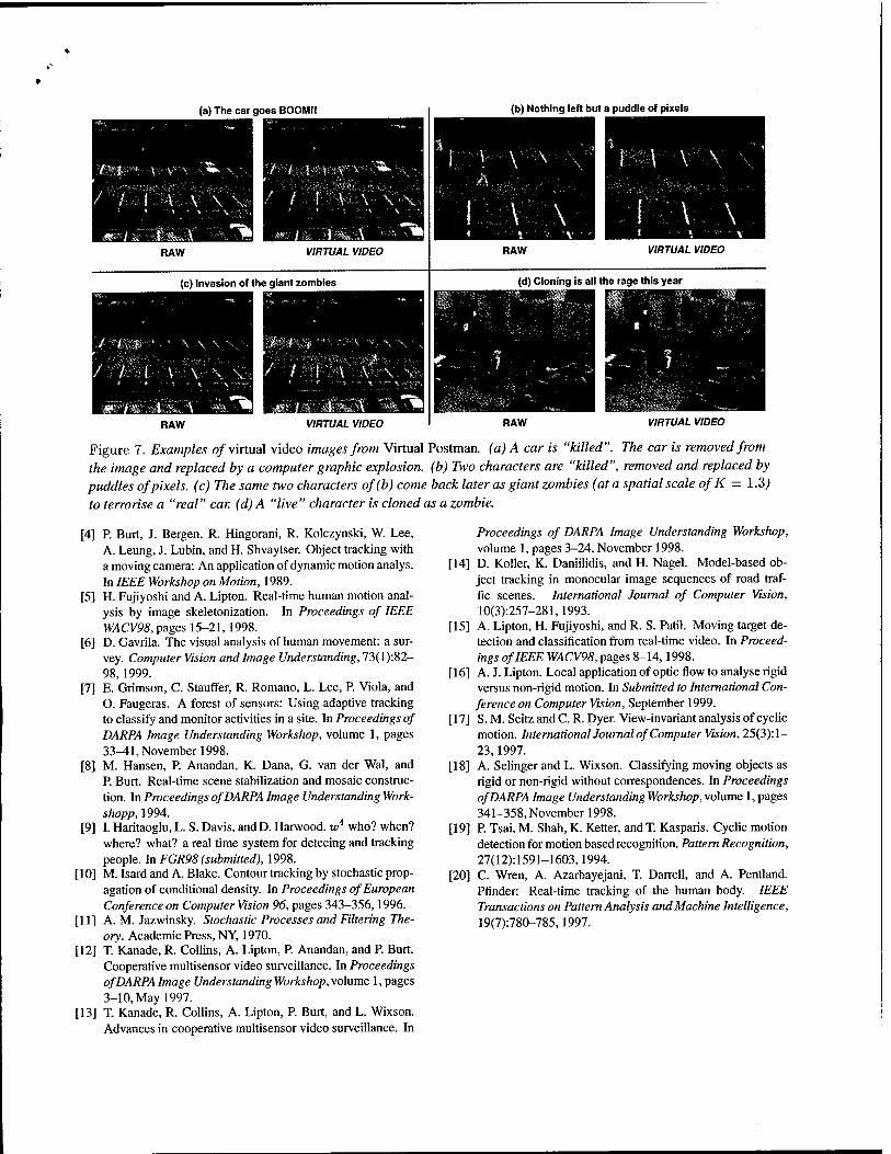
(a) The car goes BOOM!!

\ \ \ \ 1/ / I \ \ \

RAW

I I \ VIRTUAL VIDEO

(c) Invasion of the giant zombies

/ / i • • ' --VA \\V

/ / ! \ \ \ \ ■/ / I V \' \ v

RAW VIRTUAL VIDEO

(b) Nothing left but a puddle of pixels

\ ^

I \ \ I > ■••• \

RAW

\ V \

\ \

VIRTUAL VIDEO

(d) Cloning is all the rage this year

RAW VIRTUAL VIDEO

Figure 7. Examples of virtual video images from Virtual Postman, (a) A car is "killed". The car is removed from the image and replaced by a computer graphic explosion, (b) Two characters are "killed", removed and replaced by puddles of pixels, (c) The same two characters of(b) come back later as giant zombies (at a spatial scale ofK = l .3)

to terrorise a "real" car. (d) A "live" character is cloned as a zombie.

[4] P. Burt, J. Bergen, R. Hingorani, R. Kolczynski, W. Lee, A. Leung, J. Lubin, and H. Shvaytser. Object tracking with a moving camera: An application of dynamic motion analys. In IEEE Workshop on Motion, 1989.

[5] H. Fujiyoshi and A. Lipton. Real-time human motion analysis by image skeletonization. In Proceedings of IEEE WACV98, pages 15-21,1998.

[6] D. Gavrila. The visual analysis of human movement: a survey. Computer Vision and Image Understanding, 73(1 ):82- 98,1999.

[7] E. Grimson, C. Stauffer, R. Romano, L. Lee, P. Viola, and O. Faugeras. A forest of sensors: Using adaptive tracking to classify and monitor activities in a site. In Proceedings of DARPA Image Understanding Workshop, volume 1, pages 33^11, November 1998.

[8] M. Hansen, P. Anandan, K. Dana, G. van der Wal, and P. Burt. Real-time scene stabilization and mosaic construction. In Proceedings of DARPA Image Understanding Work- shopp, 1994.

[9] I. Haritaoglu, L. S. Davis, and D. Harwood. w4 who? when? where? what? a real time system for detecing and tracking people. In FGR98 (submitted), 1998.

[10] M. Isard and A. Blake. Contour tracking by stochastic propagation of conditional density. In Proceedings of European Conference on Computer Vision 96, pages 343-356,1996.

[11] A. M. Jazwinsky. Stochastic Processes and Filtering The- ory. Academic Press, NY, 1970.

[12] T. Kanade, R. Collins, A. Lipton, P. Anandan, and P. Burt. Cooperative multisensor video surveillance. In Proceedings of DARPA Image Understanding Workshop, volume 1, pages 3-10, May 1997.

[13] T. Kanade, R. Collins, A. Lipton, P. Burt, and L. Wixson. Advances in cooperative multisensor video surveillance. In

Proceedings of DARPA Image Understanding Workshop, volume 1, pages 3-24, November 1998.

[14] D. Koller, K. Daniilidis, and H. Nagel. Model-based object tracking in monocular image sequences of road traffic scenes. International Journal of Computer Vision, 10(3):257-281,1993.

[15] A. Lipton, H. Fujiyoshi, and R. S. Patil. Moving target detection and classification from real-time video. In Proceed- ings of IEEE WACV98, pages 8-14,1998.

[16] A. J. Lipton. Local application of optic flow to analyse rigid versus non-rigid motion. In Submitted to International Con- ference on Computer Vision, September 1999.

[17] S. M. Seitz and C. R. Dyer. View-invariant analysis of cyclic motion. Internationaljournal of Computer Vision, 25(3):1- 23,1997.

[18] A. Selinger and L. Wixson. Classifying moving objects as rigid or non-rigid without correspondences. In Proceedings of DARPA Image UnderstandingWorkshop,-vo\ume 1, pages 341-358, November 1998.

[19] P. Tsai, M. Shah, K. Ketter, and T. Kasparis. Cyclic motion detection for motion based recognition. Pattern Recognition, 27(12):1591-1603,1994.

[20] C. Wren, A. Azarbayejani, T. Darrell, and A. Pentland. Pfinder: Real-time tracking of the human body. IEEE Transactions on Pattern Analysis and Machine Intelligence, 19(7):780-785,1997.

Documents

A System for Video Surveillance and Monitoring CMU VSAM ... · A System for Video Surveillance and Monitoring CMU VSAM Final Report * Takeo Kanade, Robert T. Collins, Alan J. Lipton,