A Survey and Discussion of Memcomputing Machines

Daniel Saunders

November 23, 2016

Abstract

This paper serves as a review and discussion of the recent works on memcomputing. In particular, the

universal memcomputing machine (UMM) and the digital memcomputing machine (DMM) are discussed.

We review the memcomputing concept in the dynamical systems framework and assess the algorithms

offered for computing NP problems in the UMM and DMM paradigms. We argue that the UMM is a

physically implausible machine, and that the DMM model, as described by numerical simulations, is no

more powerful than Turing-complete computation. We claim that the evidence for the resolution of P

vs. NP is therefore inconclusive, and conclude that the memcomputing machine paradigm constitutes

an energy efficient, special-purpose class of models of dynamical systems computation.

1 Introduction

The memcomputing model recently introduced by di Ventra, et al. [1] provides a novel way of harnessing

nonlinear circuits to perform massively parallel computation. Generally, a memcomputing device can be

thought of as a network of memprocessors, simple computing devices which, when wired together, take

advantage of their “collective state” in order to compute functions in a massively parallel manner. The device

is accompanied by a control unit, which is used to signal computing instructions to the memprocessors. It is

important to note that the control unit itself does not perform any computation, in terms of floating-point

operations or bit-wise manipulations. After an instruction specified by the control unit has been carried out,

the state of the network of memprocessors can be read as the output of the computation step. Memprocessors

compute with and in memory, such that each memprocessor has its own residual memory effects (granted by

its memristive makeup) and may interact with up to as many as every other memprocessor in the network.

A memcomputing device therefore has no need for a separate CPU, and may save on computation time (due

to overcoming the von Neumann bottleneck [8]) and energy expenditure. It is natural to cast the machine as

a dynamical system, whose constituent elements are memprocessors, and whose dynamics are derived from

the structure of their interconnections and a few simple governing rules.

It is claimed in [3] that the digital memcomputing machine is able to solve general NP problems with only

polynomial resources (i.e., polynomial time, space, and energy use), boasting identical computational power

to that of a nondeterministic Turing machine (NTM). It is further argued that there exists a simulation

of the digital memcomputing machine (a system of differential equations) implementing an NP algorithm

which has only a polynomial blowup in running time, and may therefore resolve the question of P vs. NP

in favor of equality. This is supposing, however, the correctness of the algorithms which are said to solve the

NP problems, their polynomial worst-case running time, and the correct polynomial time simulation of the

1

operation of the memcomputing machine. This claim is surprising, as the P vs. NP problem has been open

for decades, withstanding a great deal of complexity theory research. This paper therefore serves to provide

skepticism on this point, and to consider the relation of the memcomputing concept to classical computation

models in general.

The paper is organized as follows. In section 2, we introduce memristors and memristive circuit hardware,

first proposed by Chua [10], and later developed by Di Ventra, et al. [9]. In section 3, we give an overview

of the memcomputing concept and properties of memcomputing machines. In section 4, we formally define

the memprocessor. In section 5, Universal Memcomputing Machines (UMMs) are introduced, and their

application to NP problems is discussed. Section 6 is devoted to the UMM hardware implementation of the

SUBSET ´ SUM problem, and the problems that occur when attempting to scale it to large input sizes.

In Section 7, we introduce the Digital Memcomputing Machine (DMM), compare it with standard models

of computation, and discuss the conditions it must satisfy as a dynamical system. In section 8, we discuss

the proposed implementation of the DMM and the circuit equations that result. Section 9 is devoted to the

study of the algorithms for the solution to NP problems, as well as a review of the evidence in favor of P

vs. NP . Finally, Section 10 is devoted to conclusions.

2 Memristors and Memristive Elements

The first description of the memristor was given by Chua [10] in 1971, then motivated by the gap in the

definitions of the relationships between each pair of the four fundamental circuit variables (current, voltage,

charge, and flux-linkage). Of the possible six pairings, only the relationship between flux-linkage φ and

charge q had gone without characterization. It was defined in terms of a new basic circuit element, the

memristor, so named for its behavior, which is not unlike that of a nonlinear resistor with memory. At this

point in its history, the device was only a theoretical concept, and it was not until 2008 until “the missing

memristor was found” by HP Labs scientists [25].

A memristor is defined by the relation fpq, φq “ 0, and is said to be charge-controlled (flux-controlled)

if this relation can be defined in terms of a single-valued function of the charge q (flux-linkage φ). Though

a memristor behaves like a normal resistor at any given instant in time, t0, its resistance (conductance)

depends on the entire past history of current (voltage) across the device. Once the voltage or current over

time is specified (vptq, iptq), this circuit element behaviors like a linear time-varying resistor, which effectively

describes the memory effects the memristor exhibits. It was shown that the element demonstrates behavior

unique from that of standard resistors, capacitors, and inductors, and with these properties there are a

number of memristive circuit applications which cannot be recognized with standard RLC networks alone.

The nonlinear dynamical behavior of a memristor is characterized by a pinched hysteresis loop, which is

what underlies the memory effects seen in memristive behavior.

The new circuit element potentially has profound implications for the construction of new, more efficient

circuit hardware at the nanoscale. One exciting feature of certain realizations of the memristor is that

it acts as a non-volatile memory; this means that the device retains its internal state (say, resistance or

capacitance), even when it is disconnected from power. In this way, the memristor represents a passive and

non-volatile memory element which is capable of computation due to the fast switching times of its internal

state variable(s).

Di Ventra et al. [9] extended the concept of memristive systems to include capacitors and inductors with

2

memory effects, known as memcapacitors and meminductors. This work gave analogous definitions to the

capacitive and inductive elements and described their dynamical properties. Collectively, these elements

with memory effects are known as “memelements”. Using these elements (in particular, the memristor), Di

Ventra, et al [11] describes a new, massively parallel approach to solving mazes. As mazes are prototypical

graphs, it is natural to extend this method to solve graph theoretic queries. Indeed, the memcomputing

machine approach described in Section 9 is particularly amendable to such problems. Another application

of these devices is in simulating neuronal synapses [26]; in particular, implemented as threshold devices,

memristors can learn functions by switching to a high or low state of resistance based on the history of its

inputs.

3 The Memcomputing Concept

A major motivation for the adoption of the memcomputing model is the fundamental limitations of the

von Neumann computer architecture. This construction specifies a central processing unit (CPU) that is

separate from its memory, and therefore suffers a under a constraint known as the von Neumann bottleneck

[8]; namely, the latency in busing data between the CPU and memory units. The busing action may also

waste energy that might otherwise be conserved with a more efficient architecture [8].

Parallel computation was an important first step in decreasing the amount of time needed to compute

certain problems, but since all parallel processors must communicate with one another to solve a problem, a

considerable amount of time and energy is required to transfer information between them [8]. This latency

issue thus calls for a fundamentally different architecture, in which data are manipulated and stored on the

same physical device. Additionally, parallel computation has its limits; indeed, if NC ‰ P (as is widely

believed), then there exist problems that are “inherently sequential”, which cannot be sped up significantly

with parallel algorithms [13]. Furthermore, in building parallel systems, there is a fundamental trade-off

between the amount of hardware we are willing to operate and the amount of time we are willing to expend,

which acts as a strong physical limitation on our ability to scale parallel processing.

The paradigm of memcomputing has recently been introduced as an attempt to answer these problems [1].

Memcomputing machines compute “with and in” multi-purposed memory and computation units, thereby

avoiding the transfer latency between the main memory and CPU. These machines are built using memristive

systems, as explained above, and therefore exhibit time non-locality (memory) in their response functions at

particular frequencies of inputs. The fundamental processing elements used by the machines are known as

memprocessors, which may be composed of the memristors, memcapacitors, and meminductors mentioned in

the previous section. Since the family of memristive components are passive circuit elements, implementing

the machines with these devices may save on energy, as the pinched hysteresis loop characterizing memristive

behavior implies that no energy needs to be stored during a computation.

A memcomputing machine is composed of a network of memprocessors, otherwise known as the compu-

tational memory, which is signaled by a control unit, which is responsible for specifying the input to the

machine. The control unit does not perform any computation itself, thereby eliminating the need to bus

information between itself and the memory. Thus, the input data is applied directly to the computational

memory via the control unit. The output of the machine can be read from the nodes of the network of

memprocessors at the end of the machine’s computation.

3

We now discuss the three main properties that these machines are said to possess. The terminology used

below is taken from references [1] - [3].

3.1 Intrinsic Parallelism

Intrinsic parallelism refers to the feature in which all memprocessors operate simultaneously and collec-

tively during the machine’s computation. Instead of solving problems via a sequential approach as in the

Turing paradigm, we can allegedly design memcomputing algorithms which solve problems in fewer steps

by taking advantage of the massive parallelism granted by the computation over the collective state of the

memprocessors in the computational memory. The idea that this intrinsic parallelism may grant us non-

trivial computation speed-up is contested in the computational complexity community [6], but indeed, it is

not unlikely that memcomputing machines could grant constant-factor speedups over standard Von Neu-

mann machines, especially considering the fast switching times of the memristive devices used to build these

machines.

3.2 Functional Polymorphism

Functional polymorphism is the idea that a memcomputing machine’s computational memory can be

re-purposed to compute different functions without modifying its underlying topology. This is similar to

allowing a Turing machine access to different programs, or transition functions, in that the signal applied

to the current state of the machine determines its operation. The machine’s current state, along with the

signals applied to the memprocessors, determines the state of the machine at the next computation step.

This feature allows the machine to compute different functions by applying the appropriate signals. Thus,

the control unit may be fed by a stream of input data, or operate conditionally depending on the state of

the computational memory.

3.3 Information Overhead

Information overhead allegedly allows the machine to store and compress more than a linear amount of

data as a function of the number of memprocessors in the network, because of the physical coupling of the

individual elements. This amount is supposedly larger than that possible by the same number of uncoupled

processing elements. Information is not explicitly stored in the connections of the computational memory,

but rather, there is an implicit embedding of information as a property of the computation on the collective

state. This information storage is accomplished by the non-linearity of the memristive response function

internal internal to these devices.

4 Memprocessors

All definitions and notation are taken from [1].

Definition 5.1: A memprocessor is defined by the four-tuple px, y, z, σq, where x is the state of the

memprocessor (taken from a set of states, which may be a finite set, a continuum, or an infinite set of

4

discrete states), y is an array of internal variables, z is an array of connecting memprocessor elements, and

σ is an operator which defines the evolution of a memprocessor, given by

σrx, y, zs “ px1, y1q, (1)

where x1, y1 are the update state and internal variables of the memprocessor, respectively.

When two or more memprocessors are connected, they form a network whose state we denote by x,

a vector which holds the states of all memprocessors in the network. We denote by z the union of all

connecting variables between memprocessors. The evolution of the entire computational memory is given by

the evolution operator Ξ, which is defined by

Ξrx,y, z, ss “ z1, (2)

where y is the union of all the connecting variables of the network, and s is the array of signals provided

by the control unit at the connection of processors that act as external stimuli. The total evolution of an

n-memprocessor network is given by

$

’

’

’

’

’

’

&

’

’

’

’

’

’

%

σrx1, y1, z1s “ px11, y

11q,

...

σrxn, yn, zns “ px1n, y

1nq,

Ξrx,y, z, ss “ z1.

The operators σ and Ξ can be interpreted as either in discrete or continuous time, the discrete time

containing the artificial neural network (ANN) model, whereas the continuous-time operators represents a

more general class of dynamical systems.

5 Universal Memcomputing Machines

We describe the universal memcomputing machine (UMM). A claim of Di Ventra, et al. [1] is that these

machines are strictly more powerful than Turing machines. However, if we can successfully build these

machines, then we have a counterexample to the physical Church-Turing thesis [17], which states that any

reasonable physical model of computation is equivalent in power to the Turing machine. If this is true,

than this contribution is certainly the most significant result of the memcomputing works. We also give

the argument, found in [1], that UMMs are allegedly capable of solving NP problems in polynomial time,

taking advantage of the machine’s computation over collective states. We will see the problems inherent to

its physical construction towards the end of this section.

5.1 Definitions

We assume a basic familiarity with Turing machines and the complexity classes P and NP . For a refer-

ence on these concepts, please see [13].

Definition 6.1: A UMM is defined as the following 8-tuple:

5

pM,∆, P, S,Σ, p0, s0, F q, (3)

where M is the set of possible states of a single memprocessor (this may be a finite set, a continuum,

or an infinite discrete set of states), ∆ is a set of transition functions the control unit commands, formally

written as

δα : MmαzF ˆ P ÑMm1α ˆ P 2 ˆ S, (4)

where mα is the number of memprocessors read by (used as input for) the function δα, and m1α is the

number of memprocessors written to (used as output for) the function δα. P is the set of arrays of pointers

pα that select the memprocessors called by the function δα, S is the set of indexes α, Σ is set of initial states

of the memprocessors (written by the control unit at the beginning of the computation), p0 P P the initial

array of pointers, s0 P S the initial index α, and F ĎM the set of final states.

It is discussed in [1] that these machines can implement the actions of any given Turing machine by

embedding the state of the machine in the network of memprocessors and applying its transition function

via the control unit accordingly, thereby proving their Turing universality.

5.2 UMM Computation of NP-Complete Problems

Informally, a problem is NP -Complete if it is both in NP and there exists some “efficiently computable”

reduction from every other problem in NP to it [13]. Consider an arbitrary NP -Complete problem, and the

computation tree of the non-deterministic Turing machine (NTM) used to solve it. Since the problem is in

NP , the depth of the tree must be some polynomial function of the input length, ppnq. At each iteration,

we can assume that the computation tree branches into at most a constant number of nodes (corresponding

to the machine’s non-unique transition function), M , of NTMs. So the total number of nodes in the tree

grows exponentially with the depth of the tree, bounded above by Mppnq. This means that a deterministic

Turing machine would have to search, in the worst case, an exponentially large tree in order to decide an

instance of the problem.

Consider a UMM with the following scheme: The control unit sends an input signal to a group of

memprocessors encoding the i-th iteration of the solution tree, to compute the i+1st iteration in one step.

The control has access to a set ∆ of functions δ, where α “ 1, ..., ppnq, and δrxppαqs “ px1ppα`1q, α`1, pα`1q,

where xppiq denotes the nodes of the computation belonging to iteration i and x1ppα`1q denotes the nodes

of computation belonging to iteration i ` 1. It is important to note that the number of nodes involved at

iteration i is at most M i, and that the final iteration of the algorithm will then involve at most Mppnq nodes.

Now, since each δα corresponds to a single constant-time step for the UMM, the solution to the NP

problem will be found in time proportional to the depth of the computation tree, ppnq. Though this procedure

requires only a polynomial number of steps, the necessity for an exponentially growing number of processors

causes this approach to be just as implausible as the exponential time algorithm. Indeed, this construction

can be accomplished with a exponentially growing number of Turing machines, coupled with a delegating

machine to signal the information needed for each iteration. This argument does not show that these machines

are strictly more powerful than Turing machines, as was claimed. Instead, this is a typical example of the

fundamental parallel time / hardware trade-off characteristic of models of computation [30].

6

We further note that these machines have yet to be successfully implemented at scale in hardware, and

may prove to be a physical impossibility. In a naive implementation, we require an exponentially growing

number of memprocessors in order to store the values on the computation tree of any problem in NP , thereby

thwarting the usefulness of the polynomial running time for all practical purposes.

5.3 UMM Information Overhead

We direct the read to reference [1] for the definition of information overhead in the context of UMM

computation. In this work, Di Ventra et al. explain both quadratic and exponential information overhead,

given a mathematical description of the hardware necessary to compress the information into a linear amount

of hardware. The case of quadratic information overhead is, in fact, equivalent to the scenario in which some

number of independent memprocessors are coupled with a CPU to perform a simple computation over the

values they store, and therefore is not a very interesting theoretical concept.

In the case of exponential information overhead, consider a network of n memprocessors. Each mempro-

cessor can store data in its internal state. We describe the internal state of the memprocessor as a vector with

some number of components, and we assume the memprocessor itself is a “polarized” two-terminal device,

in that the left and right terminal, when connected to other circuit elements, interact in physically different

ways. We label the left side as “in” and right side as “out” in order to distinguish the two. Furthermore, we

assume the blank state of the memprocessor is the situation in which all components of the internal state

vector are equal to 0. Now, in order to store a single data point, we set one of the components of the internal

state different from 0, and assume that any memprocessor can store a finite number of these data points at

once. We also assume that there exists a device which, when connected to a memprocessor, can read the

data points which it stores.

To complete the construction, we include a scheme of physical interaction between any number of mem-

processors. We take two memprocessors, connected via the “out” terminal of the first and the “in” terminal

of the second. We assume the read-out device can read the states of both memprocessors at once, i.e., the

global state. We describe the global state formally as uj1,j2 “ uj1 ˛ uj2 , where uji refers to some internal

state, and where ˛ : Rd ˆ Rd Ñ Rd is a commutative, associative operation, and d “ dimpujq. It is defined

by

tuj1 ˛ uj2uh‹k “ tuj1uh ˚ tuj2uk, (5)

where ‹ : Z ˆ Z Ñ Z and ˚ : R ˆ R Ñ R are two associative, commutative operations such that

@h, h ‹ 0 “ h, @x, x ˚ 0 “ 0. Furthermore, if there are two pairs of indices, ph, kq and ph1, k1q, such that

h‹k “ h1 ‹k1, then tuj1,j2uh‹k “ tuj1 ˛uj2uh‹k‘tuj1 ˛uj2uh1‹k1 , where ‘ is another commutative, associative

operation such that x ‘ 0 “ x. Since all the operations we have defined are commutative and associative,

we can easily iterate these operations to multiple connected memprocessor units.

Now, given a set G “ ta1, ..., anu composed of n integers with sign, Di Ventra, et al. [1] defined a message

m as paσ1 ‹ ...‹aσkqYtaσ1 , ..., aσku, where tσ1, ..., σku is the set of indexes of all possible subsets of t1, ..., nu,

such that the message space M is composed ofřnj“0

`

nj

˘

“ 2n equally probably messages, each message m

having Shannon’s self-information Ipmq “ logp2nq “ n. Taking n memprocessors, for each i we set only

the 0th and aith components different from zero, and so each memprocessor encodes a distinct element of

G. If we were to read the global state of all n memprocessors using the operations defined above, we will

7

find all messages m P M . Since these n interconnected processing units have encoded 2n bits, we say that

we have achieved exponential information overhead, and it is clear that the information overhead represents

the physical coupling between memprocessor units. While the transition functions change the state of the

memprocessors themselves, information overhead is only related to the state of the memcomputing machine.

We note that this encoding of integers into single memprocessors is impractical, especially for large

integers. For this reason, the amount of hardware we require must grow linearly in the precision of the

integers we are storing, that is, the number of bits needed to represent any given integer. Further, it is not

obvious how to design hardware that will read the global state of the machine in a polynomial amount of

time or energy, especially as the set of integers we are summing over becomes large. We will see in the next

section how maintaining an exponentially large collective state quickly becomes intractable, which appears

to be the fundamental trade-off which occurs in attempting to store an exponential amount of information.

6 UMM SUBSET ´ SUM implementation

We review the memcomputing machine implementation described in [2]. For brevity’s sake, we will only

consider the machine which makes use of exponential information overhead, as the machine that makes

use of quadratic information overhead does not add anything novel in terms of computational complexity.

This is because it requires a number of memprocessors which grows exponentially with the size of the set

of integers, G, we are considering, and ignores the difficulty in storing integers of varying precision. We

discuss the computational complexity of the SUBSET ´ SUM algorithm, compare it to the complexity in

the UMM paradigm as a result of its hardware implementation, and show that this implementation requires

only a linear amount of processors, but do indeed require exponential time or energy resources in reading out

the result of the computation. For this reason, it is clear that these particular machines are not practical,

because of their inability to scale reliably with problem size.

The notation and several arguments below are taken from [1].

6.1 UMM Algorithm for SUBSET ´ SUM

Again, consider a set G “ ta1, ..., anu of n integers with sign, and the function

gpxq “ 2´nnź

j“1

p1` ei2πf0ajxq. (6)

The function gpxq is attenuated by an exponential amount, 2´n, for reasons we will discuss in a later

section, and the term f0 corresponds to the fundamental frequency, equal for every memprocessor. Thus, we

are encoding the elements of G as the integer aj terms. By expanding the above product, it is easily seen

that we can store all possible 2n ´ 1 products

ź

jPP

ei2πajx “ expri2πxÿ

jPP

ajs, (7)

where P is the set of indexes of all non-empty sets of t1, ..., nu. So, the function gpxq contains information

on all sums of all possible non-empty subsets of G.

Consider the discrete Fourier transform (DFT):

8

F pfhq “ Ftgpxqu “1

N

Nÿ

k“1

gpxkqei2πfhxk . (8)

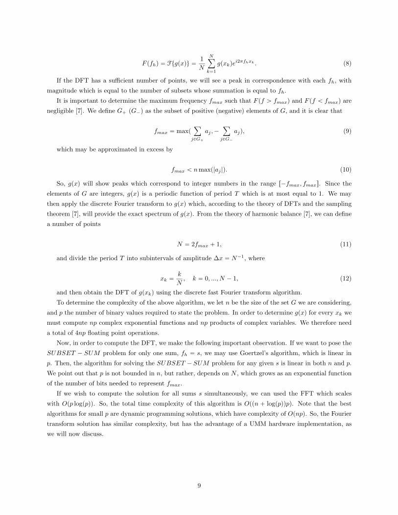
If the DFT has a sufficient number of points, we will see a peak in correspondence with each fh, with

magnitude which is equal to the number of subsets whose summation is equal to fh.

It is important to determine the maximum frequency fmax such that F pf ą fmaxq and F pf ă fmaxq are

negligible [7]. We define G` (G´) as the subset of positive (negative) elements of G, and it is clear that

fmax “ maxpÿ

jPG`

aj ,´ÿ

jPG´

ajq, (9)

which may be approximated in excess by

fmax ă nmaxp|aj |q. (10)

So, gpxq will show peaks which correspond to integer numbers in the range r´fmax, fmaxs. Since the

elements of G are integers, gpxq is a periodic function of period T which is at most equal to 1. We may

then apply the discrete Fourier transform to gpxq which, according to the theory of DFTs and the sampling

theorem [7], will provide the exact spectrum of gpxq. From the theory of harmonic balance [7], we can define

a number of points

N “ 2fmax ` 1, (11)

and divide the period T into subintervals of amplitude ∆x “ N´1, where

xk “k

N, k “ 0, ..., N ´ 1, (12)

and then obtain the DFT of gpxkq using the discrete fast Fourier transform algorithm.

To determine the complexity of the above algorithm, we let n be the size of the set G we are considering,

and p the number of binary values required to state the problem. In order to determine gpxq for every xk we

must compute np complex exponential functions and np products of complex variables. We therefore need

a total of 4np floating point operations.

Now, in order to compute the DFT, we make the following important observation. If we want to pose the

SUBSET ´ SUM problem for only one sum, fh “ s, we may use Goertzel’s algorithm, which is linear in

p. Then, the algorithm for solving the SUBSET ´ SUM problem for any given s is linear in both n and p.

We point out that p is not bounded in n, but rather, depends on N , which grows as an exponential function

of the number of bits needed to represent fmax.

If we wish to compute the solution for all sums s simultaneously, we can used the FFT which scales

with Opp logppqq. So, the total time complexity of this algorithm is Oppn ` logppqqpq. Note that the best

algorithms for small p are dynamic programming solutions, which have complexity of Opnpq. So, the Fourier

transform solution has similar complexity, but has the advantage of a UMM hardware implementation, as

we will now discuss.

9

6.2 Hardware Implementation of SUBSET ´ SUM

Consider memprocessors which are allowed an infinite set of discrete states. In this case, the mempro-

cessors are allowed to take on any integer with sign. Notice that the state vector of a memprocessor uj

can be taken as the vector of the amplitudes of one of the products in (7), and so uj is such that uj0 and

ujaj = 1, with all other components equal to 0. Then the binary operations defined for memprocessors

in Section 6.3 are the standard addition and multiplication; in particular, ‹ and ‘ are sums, and ˚ is a

product. These relations show that we can implement the SUBSET ´SUM problem using a linear number

of memprocessors by making use of exponential information overhead.

Di Ventra, et al [2] then gave the following hardware scheme for implementing the UMM subset-sum

algorithm in hardware: Complex voltage multipliers (CVMs) are defined as two-port devices, the first and

second ports functioning as the “in” and “out” terminals as described in Section 6.3, respectively. These

can be built with standard electronics as seen in [2]. Each CVM is connected to a voltage generator which

applies a voltage vj “ 1` cospωjtq, where ωj is the frequency related to an element aj P G by the function

wj “ 2πaj . The state of a single CVM can be read by connecting one port to a DC generator with voltage

V “ 1, and the other port to a signal analyzer implementing the FFT. Now, by connecting the CVMs as

in Figure 11 of [2], and using a signal analyzer on the last port, one can read their collective state, which

corresponds to the solution of the subset-sum problem for a given sum s.

To understand the time complexity involved in computing with this hardware, we consider the period

T of (7). In the hardware implementation, this completely determines the amount of time necessary to

compute the collective state of the CVMs, which is bounded and independent of both n and p. However, in

order to evaluate the FFT of the collective state (7), we would in principle need a number of time points on

the order of N . This would be troublesome even for a signal analyzer, as N grows in an exponential fashion,

thereby requiring us to spend an exponential amount of time reading out the solution. For this reason, before

connecting the signal analyzer as depicted in [2], Di Ventra, et al. interpose a band-pass filter which selects

only a range of frequencies so that the time samples needed by the analyzer will be bounded and independent

of the size of G and the precision of the integers considered. This approach allows the implementation of

the subset-sum problem in hardware in a “single step”, for any integer we wish to consider. Note that in the

numerical simulation of this construction, its time complexity is dependent on the number of time points N

needed to sample the period T , which implies an exponential time algorithm for SUBSET ´ SUM .

The algorithm given is for the decision version of the subset-sum problem, known to be NP -Complete. In

order to solve the NP -Hard version of SUBSET ´SUM , in which we would like to the know the particular

subset which sums to a given sum s, the following modifications are made: To find a particular subset which

sums to s, we can read the frequency spectrum about s for different configurations of the hardware. In the

first configuration, we turn all CVMs on, and in the second, we let ω1 “ 0. If the amplitude corresponding to

s is greater than 0 we let ω1 “ 0 for the next configuration, and otherwise turn on ω1 again, and a1 “ ω1{2π

is an element of the subset we are looking for. We then iterate this procedure for all wi, each corresponding

to an element of G, for a number of times which is linear in the size of G, and find one of the subsets which

sum to s.

10

6.3 Problems with the UMM Hardware Implementation

Thanks to [5] and [6], we can present the following arguments against the scalability of the discussed

hardware implementation of the SUBSET ´ SUM problem.

We note two problems in particular. The basic idea of the memcomputing construction is in generating

waves at frequencies which encode all the sums of all the possible subsets of G, which we measure in order

to decide whether there is a wave with frequency corresponding to a given integer sum s.

The first is a problem with the fact that, in storing the sum of an exponential number of frequencies, we

will not be able to distinguish the individual frequencies making up the collective state for an exponential

amount of time. Suppose, for example, we are implement a version of the subset-sum construction with

|G| “ n “ 1000. Then, we must measure a frequency to a precision of one part in on the order of 21000. If

the fundamental frequency, f , were 1Hz, then the individual frequencies would differ by much less than the

Planck scale, and distinguishing between them would require more energy than needed to create a black hole.

On the other hand, we can escape this exponential energy blowup by letting the fundamental frequency f

be slower than the lifetime of the universe, which would instead cause an exponential blowup in the amount

of time required to perform the computation.

On the other hand, since there are an exponential number of frequencies, the magnitude of each wave

will be attenuated by an exponential amount. Consider again the case of |G| “ n “ 1000. Then, each

wave is attenuated by a factor of 2´1000. The expected amplitude on each frequency would correspond to a

tiny fraction of a single photo. It would then take exponential time to notice any sort of radiation on the

frequency which is relevant to the solution of the subset-sum problem. In an ideal machine, it will be possible

for us to read the collective state as is presented in [2], but in actual hardware, we are quickly limited by

the physical reality of noise.

For this reason, it is natural to guess that a physical realization of the UMM is impossible, limited by

the fundamental physical limitation inherent in storing an exponential number of frequencies or states.

7 Digital Memcomputing Machines

We describe the Digital Memcomputing Machines (DMMs) detailed in [3]. These machines were intro-

duced to bypass the physical limitations of the UMM hardware discussed in the previous section. We first

introduce some terminology, taken from [3]:

Definition 8.1: A Compact Boolean (CB) problem is a collection of statements that can be written as

finite system of Boolean functions. Let f : Zn2 Ñ Zm2 be a system of Boolean functions, with Z2 “ t0, 1u.

Then, a CB problem requires that we find a solution y P Zn2 , if it exists, such that fpyq “ b with b P Zm2 .

Using this terminology, we will later consider the SUBSET´SUM and FACTORIZATION problems,

which can be written as finite systems of Boolean functions, for any particular input length.

We consider two different protocols with which to solve a CB problem. The former is amendable to a

Boolean circuit implementation, while the latter has been developed for DMM computation.

Definition 8.2: Let SB “ tg1, ..., gku be a set of k Boolean functions gi : Zni2 Ñ Zmi2 , SCFS “ ts1, ..., shu

11

a set of h control flow statements, and CF the control flow which specifies the sequence of functions of SB

to be evaluated. Then, the Direct Protocol (DP) for solving a CB problem is the control flow CF , which

operates by taking y1 P Zn12 as input and returns y P Zn2 such that fpyq “ b.

The DP is the ordered set of instructions which a Turing machine executes to solve a problem. It is easy

to map the finite set of functions into a Boolean circuit, and compute the answer in a feed-forward fashion.

For example, consider the FACTORIZATION problem, in which we are given some (possibly composite)

number n P N, and, for the sake of simplicity, are tasked with finding the two prime factors p and q such

that p ˚ q “ n. Given the binary description of n P Zn12 , our CB problem requires that we find p, q P Zn12 ,

such that fpp, qq “ n, where f is the multiplication operation. It is worth noticing that the function f is not

invertible in this case (nor in many), giving rise to unique solutions only up to ordering (p ˚ q, q ˚ p), as well

as the non-existence of solutions (in the case of prime numbers).

Definition 8.3: The Inverse Protocol (IP) is that which finds the solution of a CB problem by encoding

the Boolean system f into a machine which accepts as input b, and returns some y such that fpyq “ b, if

it exists.

So, the IP is an “inversion” of the system of Boolean functions, f . Again, f is not generally invertible,

but “special purpose” machines can be designed to solve the invertible instances of CB problems.

The class of DMMs are are strict subset of UMMs, which can be easily seen via its definition:

pZ2,∆, P, S,Σ, p0, s0, F q, (13)

where the set of states a memprocessor can take is in Z2 “ t0, 1u. The key idea is that the memprocessors

may only be in one of a finite number of states after the transition functions are applied, but may take on

real-valued states during a computation step.

7.1 DMM Implementation of the Inverse Protocol

Using a DMM, we may implement either the direct or the inverse protocol. We describe the latter case,

since the first is analogous to the implementation of a Boolean circuit.

Let f be a CB problem given by a finite Boolean system. Since f is composed of Boolean functions, it is

straightforward to map it into a Boolean circuit composed of AND, OR, and NOT logic gates. In the same

way, f is implemented in a DMM by mapping its functions into the connections of the memprocessors. A

DMM may then work in either of the “test” or “solution” modes.

In the test mode, the control unit sends a signal which encodes the input to f , y. The DMM then

functions as a Boolean circuit, where the voltages along the input wires propagate in a sequential, feed-

forward fashion, and, taking the composition of the transition functions (which correspond to the Boolean

functions that have been mapped into the DMM) of the circuit (δk ˝ ... ˝ δ1)(y), the output fpyq is obtained

and compared against the expected value of the function, b. The composition of the transition functions

δ “ δk ˝ ... ˝ δ1 we call the encoding of f into the topology of the connections of the memprocessor network.

In Boolean circuit terminology, we can see that each δi function corresponds to a layer of the circuit, and so

the underlying Boolean circuit has depth k.

12

In the solution mode, the control unit sends a signal which encodes the output of the function f , b.

The first transition function δ´11 receives it as input, and, taking the composition of the inverse transition

functions (δ´1k ˝ ... ˝ δ´1

1 )(b), the DMM produces one of the possible inputs (if it exists), y. It is important

to note that the Boolean system f is not invertible in general, and so this construction does not prevent

the event that the composition of the inverse transition functions, δ´1 “ δ´1k ˝ ... ˝ δ´1

1 , is not equal to

f´1. However, δ´1 still represents the encoding of f into the connections of the memprocessors, and for

this reason, it is known as the topological inverse transition function of f , and we call the system that δ´1

represents (some g such that gpbq “ y, which may not exist as a Boolean system) the topological inverse of f .

Computation in the solution mode is not accomplished in a feed-forward fashion, but rather the dynamical

system describing the DMM’s computation will self-organize, or converge, to a solution if it exists.

7.2 Comparison With Standard Models of Computation

As we saw above, the DMM functions by encoding a Boolean system f into the connections of its

memprocessors. In order to solve an instance of f of a certain length, we must construct a DMM which is

formed by a number of memprocessors and topology which is a function of f and the size of the input. The

use of parallelism is especially important in the implementation of the IP used to solve the CB problem,

in which the individual memprocessors may interact with many others in the network. We notice that the

exact architecture of the DMM may not be unique, since there can be many different topological realizations

of the IP for a given CB problem, which is evident in the design of Boolean circuits.

Consider the case of the Turing machine, a device to which we typically provide an ordered set of

instructions to in order to perform computation. For this reason, it is obvious that the DP is most amenable

to implementation on a Turing machine, although we will see that the simulation of a DMM can be performed

on a Turing machine with only polynomial slowdown. DMMs are also quite different from artificial neural

networks [21] in that the networks do not fully map the problem to solve into the connections of the neurons.

Neural networks are in fact more “general purpose” machines, since they can be trained to solve many types

of problems. DMMs, on the contrary, require the correct choice of topology in order to solve a problem.

For this reason, the construction of a DMM for a particular input size is analogous to the construction of

a Boolean circuit. For a given problem, we can describe the infinite sequence D1, D2, ... where Di is a DMM

which computes the solution to the problem for all inputs of length i. We can in fact take the Boolean circuit

family which computes the function f , and use the connections of the logic gates to build the DMM which

computes the topological inverse of f , g, as a general-purpose method for solving problems in “reverse”.

This method is typically only useful for certain types of problems; for instance, NP -Complete problems such

as 3SAT , where we might only care about the existence of a single satisfying assignment to some number of

Boolean variables. We may iterate the solution mode procedure to obtain different satisfying results, but in

general, there is no way to tell ahead of time what input bits will result from the solution mode computation.

7.3 Information Overhead in DMMs

We review the concept of information overhead in terms of the DMM model, which was first defined in

[3]. The measure is related to the connections of the memprocessors of the machine, rather than to the data

stored in any particular units. The information stored in the processors is no greater than that which can

be stored in by a parallel Turing machine architecture. The information overhead represents the extra data

13

embedded into the topology of the connections of the memory units, as a result of the computation on the

collective state.

Definition 7.1 The information overhead is the ratio

IO “

ř

ipmUαi `m

1Uαi q

ř

jpmTαj `m

1Tαj q

, (14)

where mTαj and m

1Tαj are the memprocessors read from and written to, respectively, by the function δTαj

which is the transition function formed by the interconnection of memprocessors with topology related to the

CB problem, and mUαi and m

1Uαi are the memprocessors read from and written to by the transition function

δUαi which is formed by taking the union of non-connected memprocessors. The sums are over all transition

functions used in the computation.

Now, when using the IP, we have that δTαj “ δ´1αj , defined in the previous section. On the other hand, to

employ the DP, we use the transition function of the union of non-connected memprocessors, δUαi .

7.4 Dynamical Systems Perspective

We recast the DMM model of computation as a dynamical system in order to make use of certain

mathematical results. This formulation will allow us to give definitions of information overhead and accessible

information. A dynamical systems framework has been used before in order to discuss the computation of

artificial recurrent neural networks [21], and since these are similar to DMMs, we may extend the theory in

a natural way.

Consider the transition function δα defined previously, with pα, p1α P P as arrays of pointers to certain

memprocessors. We describe the state of the network of memprocessors with the state vector x P Zn2 . So,

xpα P Zmα2 is the vector of the states of the memprocessors selected by the array of pointers pα. The

transition function δα then acts as

δαpxpαq “ x1p1α . (15)

So, δα reads the current memprocessor states xpα and writes the new states x1p1α . We note that the

transition functions acts simultaneously on all memprocessors, changing their states all at once.

In order to understand the dynamics of the DMM, we define the time interval Iα “ rt, t ` Tαs as the

time that δα takes to perform its transition. Now, we can describe the computation of the system using

the dynamical systems framework [22]. At time t, the control unit sends a signal encoding the transition

function to the computational memory, which has state xptq. The dynamics of the DMM during the interval

Iα, between the start and finish of the transition function, is described by the flow φ [22]

xpt1 P Iαq “ φt1´tpxptqq. (16)

This means that all memprocessors interact at each instant of time in the interval Iα such that

xpαptq “ xpα (17)

14

xp1αpt` Tαq “ x1p1α (18)

For a DMM with n memprocessors, its phase space is the n-dimensional space in which xptq is a trajectory.

The information embedded in the topology of the DMM (e.g., the encoding of the Boolean system f) strongly

affects the dynamics of the DMM.

It is stated in [3] that the dynamical system which characterizes a DMM must satisfy the following

properties:

• each component xjptq of xptq has initial conditions xjp0q P X, where X is the phase space and is also

a metric space.

• For each configuration which belongs to Zm2 , we can associate one or more equilibrium points xs P X,

and the system converges exponentially to these equilibria [22].

• The stable equilibria xs P X are associated with the solution(s) of the CB problem encoded in the

network topology.

• The input / output (namely y and b in test mode or b and y in solution mode) of the DMM must be

mapped into a set of parameters p (input) and equilibria xs (output) such that there exists p̂, x̂ P Rand |pj ´ p̂| “ cp and |xsj ´ x̂| “ cx for some cp, cx ą 0 independent of ny “ dimpyq and n “ dimpbq.

If we indicate a polynomial function of n of maximum degree γ with pγpnq, then dimppq “ pγppnq and

dimpxsq “ pγxpnbq in test mode or dimppq “ pγppnbq and dimpxsq “ pγxpnq in solution mode, with γx

and γp independent of nb and n.

• Other stable equilibria, periodic orbits, or strange attractors (which we indicate with xwptq P X) which

are not associated with solution(s) of the problem may exist, but their exist is either irrelevant or may

be ignored by setting initial conditions accordingly.

• It has a compact global asymptotically stable attractor [22], which means that there is a compact subset

J of X which attracts the whole space.

• The system converges to equilbria exponentially fast starting from an initial configuration whose mea-

sure is not zero, and which can decrease at most polynomially with the size of the system. The

convergence time may only increase polynomially with the size of the system.

The last conditions implies that the phase space is completely clustered into regions which are the

attraction basins of the stable equilibria, and could possibly be periodic orbits or strange attractors, if they

exist in the system. We note that the class of systems which have a global attractor is called dissipative

dynamical systems [22]. It is shown in [3] that the DMM construction satisfies the above properties, with

the advantage that the only equilibrium points must be solutions to the topology-dependent problem.

8 DMM Implementation

In the previous section, we gave the dynamical systems properties which characterize what could be a

physical realization of a DMM. From this, it is clear that there is no mathematical limitation in supposing

that a system with these properties exists. With the goal of building a physical system that satisfies the

15

requirements of a DMM, we discuss a new type of logic gate proposed by Di Ventra, et al [3] in order to

understand how these may be assembled in a network to form a DMM.

8.1 Self-Organizing Logic Gates

We may take any known logic gate (AND, XOR, NOT , ...) and devise a “self-organizing” gate which

may work either as a standard gate (sending input and obtaining an output), or in “reverse”, wherein by

selecting an output, the gate will dynamically find an input which is consistent with the output, depending

on the gate’s logic function. This new circuit element is called a self-organizing logic gate (SOLG). An SOLG

can use all of its terminals simultaneously both as input or output, meaning that signals can go in and out of

any terminal at any instant of time. The gate changes the outgoing components of the signals dynamically,

behaving according to simple rules created to satisfy its logic relation.

An SOLG may either be in a stable configuration, where its logic relation is satisfied, and the outgoing

components of the signal remain constant over time, or an unstable configuration, in which its logic relation

is unsatisfied, and so the SOLG drives the outgoing components of the signals in order to obtain stability.

A self-organizing logic circuit (SOLC) is a circuit composed of SOLGs connected with a problem-

dependent topology. At each node of the SOLC, i.e., at each interconnection of SOLGs, an external input

can be provided, or the output can be read (i.e., the voltage at the node). We note that the topology of the

circuit may not be unique, as there are many circuits which realize the same function, being derived from

standard Boolean circuit theory. Therefore, given a CB problem f , it is straightforward to implement f into

an SOLC using Boolean relations.

8.2 SOLG Electronics

The SOLGs can be implemented using standard electronic devices. Di Ventra, et al [3] gives a universal

self-organizing gate which, provided the corresponding signal, can compute either the AND, OR, or XOR

function. This is called universal since these logic relations together form a complete Boolean basis set.

Choosing a reference voltage vc, we encode the logic t0, 1u as t´vc, vcu, and restrict our SO gates to having

fan-in two (v1, v2) and fan-out one (v0). The basic circuit elements used in the SOLC construction are

resistors, memristors, and voltage-controlled voltage generators. We discuss the last two in the following.

The standard memristor equations are as follows [1]:

vM ptq “MpxqiM ptq, (19)

C 9vM ptq “ iCptq, (20)

9xptq “ fM px, vM q, (21)

9xptq “ fM px, iM q, (22)

where x denotes the state variables(s) describing the internal state(s) of the system (we assume from now

on the existence of only one internal variable); vM and iM the voltage and current across the device. M is

a monotonic and positive function of x. One possible choice of M is the relation

Mpxq “ Ronp1´ xq `Roffx, (23)

16

which approximates the operation of a certain type of memristors, where Ron and Roff correspond to the

minimum and maximum resistances of the memristor, respectively. This model includes a small capacitance

C in parallel to the memristor which represents parasitic capacitive effects. fM is a monotonic function of vM

(iM ) for x P r0, 1s and undefined otherwise. In fact, any function which is monotonic and null for x R r0, 1s

will suffice to define a memristor. This particular choice of hardware elements is not unique, and can be

replaced with other devices; in particular, we can replace the memristor functionality with an appropriate

combination of transistors.

The voltage-controlled voltage generate (VCVG) is a linear voltage generator controlled by the voltages

v1, v2, and v0. The output voltage is given by a linear combination of these variables of the form

a1v1 ` a2v2 ` a0v0 ` dc, (24)

whose parameters (ai’s and dc) are defined in Table I of [3], and are chosen to satisfy the relations of

the constituent gate (AND, OR, or XOR). The choice of parameters strongly effects the dynamics of the

DMM, and can be summarized as either (1) if the configuration of a gate is correct, i.e., the logic relation

is satisfied by the incoming voltages, then no current flows from any terminal. We say that the gate is in

equilibrium, or (2) otherwise, a current of the order vc{Ron flows from the each gate with sign opposite to

the voltage impinging on the terminal. Connecting these gates together in a network, these requirements

force each gate to satisfy its logic relation, since their correct configurations are stable equilibrium points.

With the above SOLC implementation of the DMM, we may not always prevent the existence of stable

solutions which aren’t properly encoded by ˘vc, and therefore do not translate into a Boolean solution.

For this reason, at each terminal (except for the inputs to the SOLC) is connected a Voltage-Controlled

Differential Current Generator (VCDCG). This device ensures ˘vc as the only possible stable solutions at

the end of any computation. To see how this device works, and the equations governing its behavior, see

reference [3].

9 DMM Implementation of FACTORIZATION

Without loss of generality, consider n “ pq, where p and q are prime numbers. The FACTORIZATION

problem requires that we find p, q such that pq “ n. In order to cast this as a CB problem, f , we may

write the product of two numbers in binary using a closed set of Boolean functions. Thus, we can write the

product as fpyq “ b, where b is the bit representation of the integer n, and y is the bits of the primes p, q.

Clearly, f is only unique up to the ordering of factors.

9.1 Resource Expenditure

Now, we give the argument that this problem can be solved in the memcomputing framework using

only polynomial resources, i.e., circuit hardware, time, and energy expenditure. The SOLC computing the

factorization of integers of 6 bits is sketched in [3]. The inputs are given by voltage generators giving the

critical voltages ˘vc encoding the bits of the integer n. We say that the collection of voltage generators is

the control unit of the DMM.

The wires of the circuit at the same potential, indicated as pj , qj , are the solutions to the problem once

the SOLC has self-organized, encoding the bits of the prime factors p and q. To read the output of the SOLC,

17

we measure the voltage along these wires, and because the values of the potentials on all wires can only be

˘vc after self-organization, there is no problem with precision in reading the output. This is a departure

from the UMM hardware implementation, where noise was a restrictive difficulty for large inputs.

As for the space complexity of the circuit, the size of the circuit grows quadratically in the input size. In

fact, the construction relies on the Boolean circuit for integer multiplication, and, performing an “inversion”

on this multiplication circuit and using the SOLGs and associated hardware, we obtain the SOLC used for

implementing the factoring algorithm in the IP. Based on the analysis in [3], the circuit converges expo-

nentially fast to the equilibria (which are the prime integer solutions to the problem), in a time supposedly

polynomial in |n|. Since the energy usage of the circuit depends linearly on the time it takes to find the equi-

libria and the number of gates in the circuit, if the running time is polynomial, then the energy expenditure

is also bounded by a polynomial function.

In order to simulate the system of ODEs which govern the behavior of the circuit, we need a bounded time

increment dt which is independent of the size of the circuit, and dependent only on the fastest time constant

governing its function. This depends on the nature of the hardware which is simulated. If there exists a

solution to the prime factorization problem, and the SOLC fulfills the dynamical systems requirements of

Section 8.4, then the problem can allegedly be solved in hardware using only polynomial resources. This last

claim has serious implications for computational complexity theory, and for this reason, we will argue in a

later section for the implausibility of this result.

If the integer we are considering is a prime number, then there is no solution to the factorization problem,

and the SOLC will never be in equilibrium. This is also true for the case in which the number of bits of the

factors used to build the circuit is smaller than the actual length of the factors, |p|, |q|. In order to avoid

this last case, we choose the bit string lengths |n| ´ 1 and t|n|{2u (or the reverse), which guarantees that if

p and q are prime integers, the solution is unique, and that the trivial solution n “ nˆ 1 is impossible.

9.2 Numerical Simulations

In [3], the SOLCs for integer factorization were implemented into the NOSTOS (NOnlinear circuit and

SysTem Orbit Stability) simulator [28]. For the sake of simplicity, the SOLCs were restricting to having

outputs of equal length. Circuits of several input sizes were built in this fashion, and the simulations were

performed by starting at a random initial configuration of the internal variables x and gradually switching

on the voltage generators. After a short time, all terminals approach the critical voltage ˘vc, encoding the

logical 0 and 1. When they have converged to these stable points, they are necessarily satisfying all gate

relations at once, and so the SOLC has found a solution to the problem.

Di Ventra, et al [3] have gotten positive results for this problem for integers of length up to 18 bits.

This 18-bit case requires the simulation of a dynamical system with on the order of 11,000 variables (the

numerical values of tvM , x, iDCG, su), and it is easy to see that this constitutes an enormous phase space

where, remarkably, only equilibria are to be found. Though encouraging evidence, this does not prove the

absence of unrelated limit cycles or strange attractors for all problem sizes. Indeed, we cannot say anything

definite about the correctness of this dynamical systems algorithm’s behavior asymptotically, since we have

only empirical evidence of its correct behavior for inputs of at most 18 bits. Although the SOLC algorithm

appears to converge in time polynomial in the length of its input, for these cases, this may be a consequence

of the polynomial time average-case complexity of these short instances of FACTORIZATION , or, by

18

reduction, SAT .

On the other hand, when given a prime number as input, the trajectories of the SOLC do not find

equilibria. Since we know that the dynamical system governing the circuit has a global attractor, these

trajectories must be characteristic of some complex limit cycle or strange attractor.

The reader may refer to [3] to find a similar SOLC implementation of the SUBSET ´ SUM problem.

9.3 Discussion on P vs. NP

The FACTORIZATION and SUBSET ´ SUM problems were solved in [3] by first mapping these

NP problems into the NP -Complete problem SAT , and subsequently mapping the SAT formula into the

connections of the SOLC. Similarly, we can take any problem inNP and, after performing its polynomial-time

reduction to SAT , we can map the problem into the connections of an SOLC. So, we have a general-purpose

framework for implementing NP ´Hard problems within the DMM paradigm.

We will now review the arguments given in [3] for the evidence for the positive resolution of P “ NP .

The first result that is relevant to this problem are the constraints given in Section 7.4, which constitute a

DMM able to solve NP problems using only polynomial resources. The polynomial convergence time of the

system is questionable, as the absence of limit cycles or strange attractors has not been proved, and their

presence may cause the running time to grow at an exponential rate, after having to “kick” the system some

number of times related to the exponential number of configurations the machine’s SOLG terminals could

take. However, it is claimed in [3] that the system requires only a number of kicks linear in the size of the

circuit.

The time resources needed to simulate SOLCs can be quantified by the number of floating-point operations

need to solve the system of ODEs given by (38). Using a forward integration method, the number of floating-

point operations needed depends linearly on the dimension of the system variables, x, and also depends on

the minimum time increment, dt, used to integrate with respect to the total computation time; in other

words, this depends linearly on the number of time steps Nt. Further, it is argued in [3] that the number of

variables needed to simulate the circuit scales polynomially with the size of the input, and simply depends

linearly on the number of logic gates (AND, OR, XOR) needed to encode the problem’s corresponding SAT

instance.

The number of time steps, Nt, needed to complete the computation has a double bound. The first depends

on the minimum time increment of the SOLC, dt, and the second on the minimum period of simulation Ts.

The first is independent of the size of the SOLC, and depends only on the shortest time constant of the

circuit. This means that this depends on the nature of the hardware devices we are simulating. On the other

hand, Ts can depend on the size of the dynamical system which represents the SOLC. It is the minimum

time we need to find the equilibria, which is related to the largest time constant of the circuit. Di Ventra,

et al. [3] gave an argument for the polynomial growth of this time constant, but it seems possible that the

larger time constants of this dynamical system grow exponentially quickly, as the system exhibits exponential

sensitivity to initial conditions.

The claim is that, from the polynomial time scaling of the numerical simulations given in [3] and the

absence of strange attractors and periodic orbits, this is strong evidence for the correctness of the dynamical

systems algorithm. However, these simulations have only been shown to work for inputs of at most 18 bits,

which is meager empirical evidence when considering the 1024-bit keys which govern the security of the RSA

19

encryption scheme. Indeed, many NP researchers have been led astray by the promise of polynomial scaling

algorithms for relatively small problem instances which turn out to require exponential time in the limit.

So, the evidence for the polynomial time memcomputing solution of problems in NP should be taken with a

grain of salt, and we should expect that these will require exponential time in the worst case, i.e., for certain

“hard” instances of NP problems.

10 Conclusions

We have surveyed the memcomputing model of computation, including the definitions of both the univer-

sal and digital models, their hardware implementations, and their physical plausibility with scale. Though

the dynamical systems picture and computation over a collective state are interesting contributions, it is

unclear from the DMM discussion where these machines can be numerically simulated on a Turing machine

without a significant amount of overhead. Investigating this question with difficult prime factorization in-

stances may provide more insight. Implementing these machines in hardware, however, may afford nontrivial

speedups and energy savings because of the continuous and collective nature of the machine’s computation,

and the fast switching times and passivity property of the memristor hardware.

The question of P vs. NP remains unanswered without proofs of the correctness and polynomial running

time of the FACTORIZATION or SUBSET ´SUM algorithms, and the relative ease with which we can

implement the collective state computation within the Turing paradigm is negative evidence in and of itself of

the implausibility that this has proved P “ NP . Since analog computation is not explicitly being harnessed

here (unless it has been “swept under the rug”, as with the analog behavior of the memristor hardware

simulated on digital hardware), and since the general consensus is that the question will resolve as P ‰ NP

[13], there is little reason to believe that these machines have solved the long-standing problem. The most

immediate contribution here is perhaps the dynamical systems algorithm for the solution to NP problems,

which, if correct, seems to be an interesting SAT solver, and, at best, a platform for which to continue

investigation into the question of P vs. NP within the analog computation paradigm.

The most pressing issue is the proof of the absence of limit cycles and strange attractors unrelated to the

solutions of the problem being solved. Further, a detailed analysis of the worst-case running time should help

in settling the question of how this framework bears on the question of P vs. NP . It is rather straightforward

to implement the DMM as a SAT solver, and experimenting with these on difficult instances of the problem

could shed light on the dynamical behavior of the SOLC circuits in the case of large, difficult SAT instances.

Implementing a DMM as a “general purpose” machine is also desirable, since building new hardware for

each problem instance length will be expensive. The development of new dynamical systems algorithms or

extensions of the DMM construction will be crucial in understanding how certain classes of problems can be

solved within the dynamical systems framework, and in this regard, there is much work to be done.

11 Acknowledgments

We thank professors Fabio L. Traversa and Massimiliano Di Ventra for helpful discussion and clarifica-

tions, and professors Hava T. Siegelmann, David A. Mix Barrington, and Scott Aaronson for their invaluable

insights.

20

References

[1] Traversa, Fabio Lorenzo, and Massimiliano Di Ventra. “Universal Memcomputing Machines.” IEEE

Trans. Neural Netw. Learning Syst. IEEE Transactions on Neural Networks and Learning Systems 26.11

(2015): 2702-715. Web.

[2] Traversa, F. L., C. Ramella, F. Bonani, and M. Di Ventra. “Memcomputing NP-complete Problems in

Polynomial Time Using Polynomial Resources and Collective States.” Science Advances 1.6 (2015)

[3] Traversa, F. L. and Massimilian Di Ventra. “Polynomial-time solution of prime factorization and NP-hard

problems with digital memcomputing machines.” 2016 Design, Automation & Test in Europe Conference

& Exhibition (DATE), Dresden, 14-18 March 2016. Dresden: IEEE

[4] M. Di Ventra and Y. V. Pershin, “The parallel approach,”Nature Physics,vol. 9, pp. 200–202, 2013.

[5] Markov, Igor L. “A Review of ‘Mem-computing NP-complete Problems in Polynomial Time Using Poly-

nomial Resources” Cornell University Library. Cornel University Library, 22 Apr. 2015. Web. 09 May

2016.

[6] Aaronson, Scott. “Memrefuting.” Web log post. Shtetl-Optimized. N.p., 11 Feb. 2015. Web.

[7] F. Bonani, F. Cappelluti, S. D. Guerrieri, and F. L. Traversa, Wiley Encyclopedia of Electrical and

Electronics Engineering, ch. Harmonic Balance Simulation and Analysis. John Wiley and Sons, Inc.,

2014.

[8] J. Backus, “Can programming be liberated from the von neumann style?: A functional style and its

algebra of programs,” Commun. ACM, vol. 21, pp. 613–641, Aug. 1978.

[9] M. Di Ventra, Y. Pershin, and L. Chua, “Circuit elements with memory: Memristors, memcapacitors,

and meminductors,” Proceedings of the IEEE, vol. 97, pp. 1717–1724, Oct 2009

[10] Chua, L. “Memristor-The Missing Circuit Element.” IEEE Trans. Circuit Theory IEEE Transactions

on Circuit Theory 18.5 (1971): 507-19. Web.

[11] Pershin, Yuriy, Yuriy Pershin, and Massimiliano Di Ventra. “Solving Mazes with Memristors: A

Massively-parallel Approach.” Nature Precedings (2011): n. pag. Web.

[12] Cook, Stephen A. “The Complexity of Theorem-proving Procedures.” Proceedings of the Third Annual

ACM Symposium on Theory of Computing - STOC ’71 (1971): n. pag. Web.

[13] Arora, Sanjeev, and Boaz Barak. Computational Complexity: A Modern Approach. Cambridge: Cam-

bridge U, 2010. Print.

[14] Ben-Hur, Asa, Hava T. Siegelmann, and Shmuel Fishman. “A Theory of Complexity for Continuous

Time Systems.” Journal of Complexity 18.1 (2002): 51-86. Web.

[15] Ben-Hur, Asa, Joshua Feinberg, Shmuel Fishman, and Hava T. Siegelmann. “Probabilistic Analysis of

a Differential Equation for Linear Programming.” Journal of Complexity 19.4 (2003): 474-510. Web.

21

[16] Ben-Hur, Asa, Joshua Feinberg, Shmuel Fishman, and Hava T. Siegelmann. “Random Matrix Theory

for the Analysis of the Performance of an Analog Computer: A Scaling Theory.” Physics Letters A

323.3-4 (2004): 204-09. Web.

[17] Piccinini, Gualtiero. “The Modest Physical Church-Turing Thesis.” Physical Computation A Mecha-

nistic Account (2015): 263-73. Web.

[18] Turing, A. M. “On Computable Numbers, with an Application to the Entscheidungsproblem.” Annual

Review in Automatic Programming (1960): 230-64. Web.

[19] Copeland, Jack. “The Church-Turing Thesis.” NeuroQuantology 2.2 (2007): n. pag. Web.

[20] G. Goertzel, “An algorithm for the evaluation of finite trigonometric series,” The American Mathemat-

ical Monthly, vol. 65, no. 1, pp. 34–35, 1958.

[21] H. T. Siegelmann, Neural networks and analog computation: beyond the Turing limit. Springer, 1999.

[22] L. Perko, Differential equations and dynamical systems, vol. 7. Springer Science & Business Media, 3nd

ed., 2001.

[23] L. Landau and E. Lifshitz, Statistical Physics. Elsevier Science, 2013.

[24] M. Di Ventra and Y. V. Pershin, “On the physical properties of memristive, memcapacitive and me-

minductive systems,” Nanotechnology, vol. 24, p. 255201, 2013.

[25] Strukov, Dmitri B., Gregory S. Snider, Duncan R. Stewart, and R. Stanley Williams. ”The Missing

Memristor Found.” Nature 459.7250 (2009): 1154. Web.

[26] Jo, Sung Hyun, Ting Chang, Idongesit Ebong, Bhavitavya B. Bhadviya, Pinaki Mazumder, and Wei

Lu. ”Nanoscale Memristor Device as Synapse in Neuromorphic Systems.” Nano Letters Nano Lett. 10.4

(2010): 1297-301. Web.

[27] J. Hale, Asymptotic Behavior of Dissipative Systems, vol. 25 of Mathematical Surveys and Monographs.

Providence, Rhode Island: American Mathematical Society, 2nd ed., 2010.

[28] F. L. Traversa and F. Bonani, “Improved harmonic balance implementation of floquet analysis for

nonlinear circuit simulation,” AEU - Inter. J. Elec. and Comm., vol. 66, no. 5, pp. 357 – 363, 2012.

[29] J. Stoer and R. Bulirsch, Introduction to numerical analysis. SpringerVerlag, 2002

[30] Dymond, Patrick W., and Stephen A. Cook. ”Complexity Theory of Parallel Time and Hardware.”

Information and Computation 80.3 (1989): 205-26. Web.

22