A Study on the Iris Biometric Authentication

by

Seung-Seok Choi

Submitted for the Master degree

in Computer Science

at

School of Computer Science and Information Systems

Pace University

May 2005

We hereby certify that this dissertation, submitted by Seung-Seok Choi, satisfies the dissertation requirements for the Master degree in Computer Science and has been approved.

_____________________________________________-________________

Sung-Hyuk Cha Date Chairperson of Dissertation Committee _____________________________________________-________________

Charles C. Tappert Date Dissertation Committee Member _____________________________________________-________________

SungSoo Yoon Date Dissertation Committee Member

School of Computer Science and Information Systems Pace University 2005

1

Acknowledgments

I would like to express my sincere appreciation to CSIS Biometric Research Group, Drs.

Cha and Tappert and Yoon, for their continued guidance and support during my work on

this thesis

2

Abstract

This paper presents a methodology for quantitatively establishing the discriminative power

of iris biometric data. It is difficult, however, to establish that any biometric modality is

capable of distinguishing every person because the classification task has an extremely large

and unspecified number of classes. The purpose of this study is to investigate various

combinations of features, distance measures, and classifiers to find the best combination for

determining the individuality of the iris biometric. Based on this review, a proposed

methodology is used to establish a measure of discrimination that is statistically inferable. To

establish the inherent distinctness of the classes, i.e., to validate individuality, we transform

the many class problem into a dichotomy by using a distance measure between two samples

of the same class and between those of two different classes. Various features, distance

measures, and classifiers are reviewed and evaluated. For feature extraction I compare

simple binary and multi-level dimensional wavelet features. For distance measures I examine

scalar distances, feature vector distances, and histogram distances. Especially, I compare

conventional binary feature distance measures and evaluate their performance. Finally, for

the classifiers I compare Bayes decision rule, nearest neighbor, artificial neural network,

and support vector machines. The experiment of the eleven different combinations is

performed. The best one uses multi-level 2D wavelet features, the histogram distance, and a

support vector machine classifier.

3

Table of Contents

Committee Members’ Signature............................................................................................ 1

Acknowledgments ................................................................................................................... 2

Abstract.................................................................................................................................... 3

List of Figures ......................................................................................................................... 5

List of Tables ........................................................................................................................... 6

Chapter 1 Introduction.......................................................................................................... 7

Chapter 2 Dichotomy Model................................................................................................ 10

2.1. Dichotomy Transformation........................................................................................ 10

Chapter 3 Comparison: Polychotomy vs. Dichotomy....................................................... 17

Chapter 4 Experimental Procedures.................................................................................. 23

Chapter 5 Feature Extraction and Distance Measures ..................................................... 28

Chapter 6 Binary Feature Distance Measures ................................................................... 31

6.1. Basic Binary Similarity Measures.............................................................................. 31

6.2. Binary Similarity Measures with Weights ................................................................. 37

6.3. Evaluation for the Binary Feature Distance Measure……………………………….39

Chapter 7 Comparative Experimental Results .................................................................. 43

Chapter 8 Conclusions.......................................................................................................... 48

Reference................................................................................................................................ 49

4

List of Figures

Figure 1 Transformation from (a) Feature domain to (b) Feature distance domain .................. 11

Figure 2 Dichotomy transformation process.............................................................................. 14

Figure 3 (a) Type I and II errors (b) 3-D Space Distribution..................................................... 16

Figure 4 Comparison between (a) feature domain (polychotomy) perfectly classifiable and

(b) feature distance domain (dichotomy) possibly not dichotomizable ............................ 18

Figure 5 Statistical Inference in Polychotomy and Dichotomy: (a) all classes in feature

domain, (b) partial classes and a classifier in feature domain, (c) the other classes, (d)

entire population in feature distance domain, (e) a sample representative to the

population in feature distance domain, (f) another sample representative to the

population in feature distance domain .............................................................................. 19

Figure 6 Generalizability of Iris identification. ......................................................................... 21

Figure 7 Error Evaluation Experimental Setup.......................................................................... 25

Figure 8 Three-level Wavelet Transform................................................................................... 29

Figure 9 A Chronological table for binary vector similarity measures...................................... 37

Figure 10 Intra and inter distance distributions for the various similarity measures ………….40

Figure 11 Performance vs. the contribution factor σ .. ............................................................. 42

Figure 12 Samples from the IRIS database................................................................................ 43

5

List of Tables

Table 1 Performance evaluation of the similarity measures on the iris database. ..................... 41

Table 2 Eleven different models. ............................................................................................... 44

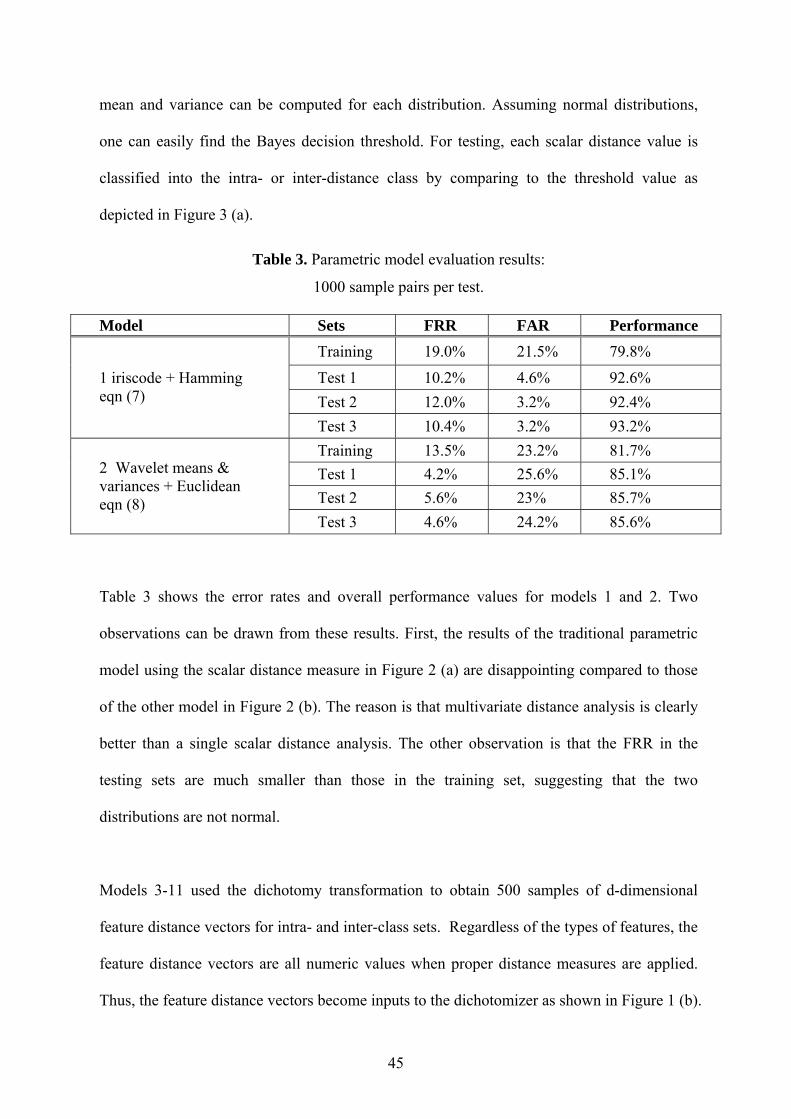
Table 3 Parametric model evaluation results: 1000 sample pairs per test... .............................. 45

Table 4 Dichotomy model performance results: 1000 independent sample pairs per test... ..... 46

6

Chapter 1

Introduction

I consider the task of establishing the distinctiveness of each individual in a population when

there is a set of measurements that have an inherent variability for each individual. This task

of establishing individuality can be thought of as showing the distinctiveness of the

individual classes with a very small error rate in discrimination. The problem is important in

many biometric and forensic science applications such as writer, face, fingerprint, speaker, or

bite mark identification. All these applications face the problem of scientifically establishing

individuality, which is motivated by court rulings [1].

Establishing a measure of uniqueness for a particular biometric is a challenging problem. A

very small error rate of a certain performance evaluation of a biometric model can be a

candidate for a measure of individuality. There are two important models in biometrics:

identification (polychotomy, one-of-many decision) and verification (dichotomy, binary

decision) [2~5]. It has been argued that the verification model is clearly more suitable than

the identification model for establishing the individuality of a biometric [3]. Consider the

many-class problem where the number of classes (individuals) is too large to be completely

observed, such as the population of a country. Most biometric identification problems fall

under the aegis of the many-class problem. Although classification techniques that assume a

fixed number of classes are not particularly useful for establishing individuality in many

class problems, some studies nevertheless use the identification model and present a

confusion matrix [6~12].

To establish the inherent distinctness of the classes, i.e., to validate individuality, we

transform the many class problem into a dichotomy by using a distance measure between two

samples of the same class and between samples of two different classes. This model allows

the inferential classification of patterns without having to observe all the classes. It is a

7

method for measuring the reliability of classification of all classes based on information

obtained from a small sample of classes drawn from the class population. In this model, two

patterns are categorized into one of only two classes; they are either from the same class or

from the two different classes. Given two biometric data samples, the distance between the

two samples is first computed. This distance measure is used as data to be classified as

positive (intra-variation, within person or identity) or negative (inter-variation, between

different people or non-identity). In [3, 4], the individuality of handwriting using the distance

statistics was shown. In this paper, I generalize the results to the iris biometric domain.

Pankanti, et al., also showed this model to establish the individuality of fingerprints [13].

Hence, the problem of iris biometric individuality is as follows. Given two iris samples, the

feature distance between the two samples is classified as intra-person (identity) or inter-

person (non-identity). We use the terms intra-person distance and inter-person distance. Two

types of errors, False Accept Rate (FAR) and False Reject Rate (FRR), are inferable to

testing sets and even to the entire population.

The proposed model has the additional advantage that it allows the use of multiple

heterogeneous features, whereas most pattern recognition techniques require that the features

be homogeneous [14]. Both continuous and non-continuous features have been studied

widely in the areas of pattern recognition [14], machine learning [15], and feature selection

[16]. In Liu and Motoda's version of the hierarchy of feature types [16], only elementary

feature types were considered: discrete ordinal and nominal, continuous, and complex.

Features observed in real applications, however, often have more complicated feature types

such as histograms, strings, etc. By taking distance measures, we are able to integrate various

types of features into one useful for many forensic science and biometric authentication

problems. Thus, the proposed dichotomy model integrates multiple features types into feature

distance scalar values [17].

8

The purpose of this paper is to investigate various combinations of features, distance

measures, and classifiers to find the best combination for determining the individuality of the

iris biometric. For feature extractions, I compare simple binary and multi-level 2D wavelet

features. For distance measures, I examine scalar distances (such as Hamming and

Euclidean), feature vector distances, and histogram distances. Finally, for the classifiers, I

compare Bayes decision rule, nearest neighbor, artificial neural network, and support vector

machines. Among the eleven different combinations tested, the best model uses the multi-

level 2D wavelet feature, histogram distance, and a support vector machine classifier.

The remainder of the paper is organized as follows: Chapter 2 illustrates the dichotomy

model which is a statistically inferable approach to establishing the individuality of a

biometric. Chapter 3 compares this model with the polychotomy model in terms of statistical

inferability. Chapter 4 explains the general procedures for the experiment. Chapter 5

presents the various features and distance measures explored for iris authentication. Chapter

6 examines the definitions of conventional binary feature distance measures and evaluates

their performance. Chapter 7 compares the experimental results of various classifiers using

different combinations of features and distance measures. Finally, Chapter 8 draws some

conclusions [18].

9

Chapter 2

Dichotomy Model

The multi-category classification problem, or Polychotomizer, is stated as follows. There are

m exemplars of each of n people (n = very large). Given a biometric exemplar, x, of an

unknown person, the task is to determine whether x belongs to any of the n subjects and if so,

to identify the person. As the number of classes is enormously large and almost infinite, I

shall demonstrate that this problem is seemingly insurmountable. To circumvent this problem,

I propose a dichotomy model that can handle the many class problem. I show how to

transform a large polychotomy problem into a simple dichotomy problem, a classification

problem that places a pattern in one of only two categories.

2.1. Dichotomy Transformation

To illustrate the transformation process, suppose there are three people, . Each person

provides three biometric data samples with two features extracted per sample. Figure 1 (a)

plots the biometric samples for the three people, where the features are real-values. To

transform this feature space into a distance vector space for real valued features, I take the

vector of distances of every feature between samples by the same person and categorize it as

an intra-person distance denoted by

},,{ 321 PPP

⊕xr . Similarly, inter-person distance distances are

obtained by measuring the distances between two different persons' biometric samples,

denoted by . Θxr

10

(a) Feature space(Polychotomy)

(b) Feature Distance space(Dichotomy)

dd1,31,3

dd1,21,2

dd2121

δδ((dd1,31,3 ,,dd2,12,1))dd1,11,1

dd2222

dd2323

dd3131

dd3232dd3333

δδ((dd1,21,2 ,,dd1,31,3))δδ((dd1,31,3 ,,dd2,12,1))

δδ((dd1,21,2 ,,dd1,31,3))

δf1

δf2

f1

f2

Figure 1. Transformation from (a) Feature domain to (b) Feature distance domain

I use subscripts of the positive ⊕ and negative ∅ symbols as the nomenclature for all

variables of intra-person distance and inter-person distance, respectively. Let ijdr denote a

feature vector corresponding to the ith person's jthΘxr biometric sample, then x⊕

r and are

obtained as follows:

| | where 1 to , and , 1 to , (1)

| | where , 1 to , and , 1 to (2)ij ik

ij kl

x d d i n j k m j k

x d d i k n i k j l m⊕

Θ

= − = = ≠

= − = ≠ =

r rr

r rr

where n is the number of people, and m is the number of biometric samples per person. Note

that the result of the dichotomy transformation is not a scalar value but a vector of distances.

Figure 1 (b) represents the transformed plot. The original feature space is transformed to a

feature distance space. For example, an intra-person distance, W (within), and an inter-

person distance, B (between), in Figure 1 (a), correspond to the points W and B in the feature

11

distance space in Figure 1 (b), respectively. Thus, there are only two categories: intra-person

distance and inter-person distance in the feature distance space.

ΘΘ = xn r⊕⊕ = xn rLet and , the sizes of inter- and intra-person distance classes, accordingly.

Fact 1 If n people provide m biometric samples each, there are positive data

samples,

nm

n ×⎟⎟⎠

⎞⎜⎜⎝

⎛=⊕ 2

2)1( −

××=Θnnmmn negative samples, and samples in total.

⎟⎟⎠

⎞⎜⎜⎝

⎛2

mn

Proof: is straight-forward. To count the inter-person distance data, we can

enumerate them as

nm

n ×⎟⎟⎠

⎞⎜⎜⎝

⎛=⊕ 2

)1())2(())1(( ××+−××+−×× mmnmmnmm L . For the first person, there are

number of other people's biometric data and he or she has m data. For the second

person, there are number of other people's biometric data that are not counted yet.

Therefore,

))1(( −× nm

))2(( −× nm

2)1(1

1

−××=××= ∑ −

=Θnnmmimmn n

i. Now, ( )! ( )( 1)

2 ( 2)!2 2mn mn mn mnn n

mn⊕ Θ

⎛ ⎞ −+ = = =⎜ ⎟ −⎝ ⎠

2( 1) ( 1)2 2

m m n nn m n n⊕ Θ− −

= + = + ▌

For example, for the handwriting data collection of [4, 5] 1000 people (statistically

representative of the U.S. population) provided exactly three samples each.

Hence, , , and there are 4,498,500 in total. 4,495,500=Θn3000=⊕n

Most statistical testing requires that the observed data be statistically independent. The

distance data is, however, not statistically independent: one obvious reason being the triangle

inequality of three distance samples of the same person. This caveat should not be ignored.

One immediate solution is to choose randomly a smaller sample from a large sample

12

obviating the triangle inequality. One can, for example, partition samples into

disjoint subsets of 500 each to guarantee no triangle inequality problem.

3000=⊕n

In the dichotomy model, we formally state the problem as follows: given two randomly

selected biometric samples, the problem is to determine whether the two exemplars belong to

the same person. Figure 2 depicts the whole process using the dichotomy transformation. Let

be the ith feature of jth biometric data. jif

First, features are extracted from both biometric data x and y: and

. Then, each feature distance is computed: . In

equations (1) and (2),

},,,{ 21x

dxx fff L

},,,{ 21y

dyy fff L )},(,),(),,({ 2211

yd

xd

yxyx ffffff δδδ L

δ is the absolute difference between two real values. However, the

features need not be real valued and could be any form such as nominal, strings, histograms,

etc. Depending on the feature type, suitable distance measures are associated, e.g.,

approximate string matching distance for string type features. Thus, the previous equations

can be rewritten as follows:

( ) where 1 to , and , 1 to , (3)

( ) where , 1 to , and , 1 to (4)ij ik

ij kl

x d d i n j k m j k

x d d i k n i k j l m

δ

δ⊕

Θ

= − = = ≠

= − = ≠ =

r rr

r rr

δwhere varies depending on feature types [17]. In all, the dichotomizer takes this feature

distance vector as the input, and outputs the decision, i.e., “same person” or “different

people.”

13

Same/different people

Distance computations

),...,,( 21x

dxx fff ),...,,( 21

yd

yy fff

),( 11yx ffδ ),( 22

yx ffδ ),( yd

xd ffδ

Dichotomizer

Scalar distancemeasure

Feature extraction

),...,,( 21x

dxx fff ),...,,( 21

yd

yy fff

Feature extraction

Bayes decisionSame/different people

(a) Parametric Verification (b) Dichotomy TransformationFRRFAR

∅

⊕

Figure 2. dichotomy transformation process

A good descriptive way to represent the relationship between two populations (classes) is to

calculate the overlap between the two distributions. Figure 3 illustrates the two distributions

assuming that they are normal. Although this assumption is invalid, we can use it to describe

the behavior of two populations figuratively without loss of generality. Assuming that we are

using a Bayes optimal classifier with equal prior probabilities, type I error (FRR) occurs

when the same person's biometric data are identified as coming from different people, and

type II error (FAR) occurs when the biometric data provided by two different people are

identified as coming from the same person as shown in Figure 3 (a).

Pr ( ( ) | ) (5)

Pr ( ( ) | ) (6)ij kl

ij kl

FRR dichotomizer d d T i k

FAR dichotomizer d d T i k

= − ≥ =

= − < ≠

r r

r r

Let X) denote the distance x position where two distributions intersect. As shown in Figure 3

(a), FRR is the right-side area of the positive distributions where the decision bound is XT)

= .

14

Suppose one must make a crisp decision and choose the intersection as a classification

boundary. Then, FRR is the probability of error that one classifies two biometric data as

different people even though they belong to a same person. FAR is the left-side area of the

negative distributions, i.e., the probability of error that one classifies two biometric data as

coming from the same person even though they belong to two different people.

As is apparent from Figure 3, the intra-person distance distribution is clustered toward the

origin, whereas the inter-person distance distribution is scattered and away from the origin.

Utilizing the fact that the intra-person distance is smaller, I design the dichotomizer to

establish the decision boundary between the intra and inter-person distances.

15

Decisionboundary

intra distance

d ( , )

inter distance

d ( , )

FAR FRR

(a)

(b)

Figure 3. (a) Type I and II errors (b) 3-D Space Distribution.

16

Chapter 3

Comparison: Polychotomy vs. Dichotomy

I now compare the dichotomy model with the polychotomy model in terms of accuracy and

statistical inference. Consider the multiple-class problem where the number of classes is

small, and one can observe many instances of each class. To show the individuality of the

classes statistically, one can cluster the instances into classes and infer the separation to the

entire population. It is an easy and valid method to establish the individuality as long as a

substantial number of instances for each class are observable. Now, consider the many class

problem where the number of classes is too large to be observed, such as the population of a

country. Many pattern identification problems, and most of the forensic science applications

mentioned above, fall under the aegis of many class problems. Although classification

techniques that assume a fixed number of classes are not appropriate for establishing

individuality in many class problems, most of the existing studies use the identification

model and present the confusion matrix [6~12].

The definition of inferential statistics is to measure the reliability of individuality for the

entire population based on information obtained from a sample drawn from the population. I

claim that the identification model is not statistically inferable for many class problems. In

this model, to draw valid conclusions, one must observe samples from every single person,

which is clearly impossible. For instance, consider handwritten alphabets and the task of

validating the individuality of alphabet shapes. If one observes instances of only the alphabet

characters {A, B, C} and draws the conclusion that all alphabet characters are distinct, this is

invalid because not all classes have been observed, and, for example, there maybe

indistinguishable version of italic I and l. Without knowing the geometrical distributions of

the unseen classes (populations), one cannot draw the statistical inference; true error of the

17

entire population cannot be inferred from the error estimate of the sample population because

there are unseen classes (the rest of the population, e.g. U.S. or other country populations).

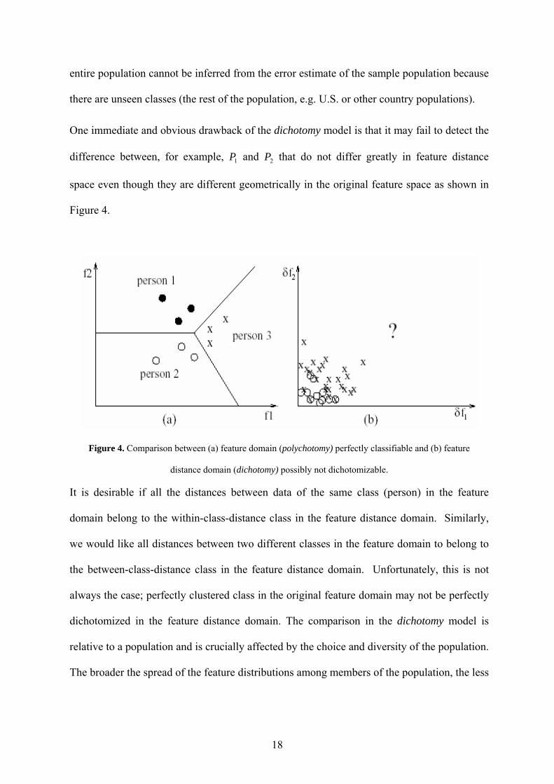
One immediate and obvious drawback of the dichotomy model is that it may fail to detect the

difference between, for example, and that do not differ greatly in feature distance

space even though they are different geometrically in the original feature space as shown in

Figure 4.

1P 2P

Figure 4. Comparison between (a) feature domain (polychotomy) perfectly classifiable and (b) feature

distance domain (dichotomy) possibly not dichotomizable.

It is desirable if all the distances between data of the same class (person) in the feature

domain belong to the within-class-distance class in the feature distance domain. Similarly,

we would like all distances between two different classes in the feature domain to belong to

the between-class-distance class in the feature distance domain. Unfortunately, this is not

always the case; perfectly clustered class in the original feature domain may not be perfectly

dichotomized in the feature distance domain. The comparison in the dichotomy model is

relative to a population and is crucially affected by the choice and diversity of the population.

The broader the spread of the feature distributions among members of the population, the less

18

we learn about detecting real differences between individuals who do not differ greatly.

However, our experimental results show that these extreme cases are rare.

The objective is to validate the individuality of biometric data statistically, but not to detect

the difference of particular instances. I are attempting to infer the individuality of the entire

population based on the individuality of a sample of n people, where n is much less than the

population. I claim that the dichotomy model is a sound and valid inferential statistics

approach.

By definition, inferential statistics measures the reliability of individuality of the entire

population based on information obtained from a sample drawn from the population. I

explain the justification of the dichotomy model using inferential statistics.

Feature Distance Domain (Dichotomy)

Feature Domain (Polychotomy)(a) (b) (c)

(f) (e)(d)

Figure 5. Statistical Inference in Polychotomy and Dichotomy: (a) all classes in feature domain, (b) partial

classes and a classifier in feature domain, (c) the other classes, (d) entire population in feature distance

domain, (e) a sample representative to the population in feature distance domain, (f) another sample

representative to the population in feature distance domain.

19

Suppose that we use the polychotomy model to validate the individuality of biometric data.

In this model, a population consists of the biometric data of every person in the population.

To draw a valid conclusion, therefore, one must observe samples from every single person,

which is impossible. If we observe only 1,000 people (classes/populations), drawing a

statistically inferential conclusion is invalid because there are unseen classes. One cannot

draw the statistical inference; true error of the entire population cannot be inferred from the

error estimate of the sample population of 1000 because there are unseen classes (the rest of

the population).

Figure 5 (a)-(c) illustrates this issue. Suppose there are only 6 people in the universe (a), and

we observe the biometric data of three people (1, 4, and 5) (b) because we assume that

observing all people is difficult. Although one can successfully discriminate among the three

people using a pattern classification or machine learning technique, the learned

polychotomizer is not suitable for the other classes, as shown in (c). Clearly, the

polychotomy model is not statistically inferable.

Transforming the US population class-classification problem into a two class problem helps

us overcome this issue, as shown in Figure 5 (d)-(f), where (d) and (e) are the dichotomy

transformed plots of (b) and (c), respectively. There are only two populations, and we can

acquire sufficient instances of each class or population. Since every new instance also maps

onto these two classes, the distribution of the sample population can be used to infer the

distribution of the entire population. Although we might do better by detecting real

differences between individuals who do not differ greatly in the polychotomy model, the

statistical inference is of primary interest and the dichotomy model is a sound and valid

inferential statistical model whereas the polychotomy one is not. As we shall see later in

section 5, as borne out by our training and testing results, only 3% of the data was

misclassified. Since misclassification error can be attributed to a number of factors such as

20

feature selection in addition to “masking”. “Masking” likely occurred in an even smaller

percentage. In all, inferring the error probability of the entire population through the

dichotomizer model is more useful than detecting real differences between individuals who

do not differ greatly from the sample population in the polychotomy model.

I further support our claim that the polychotomy (identification) model is not statistically

inferable one. When the number of classes increases, the error rate increases. In other words,

the error rate counted in the polychotomy model based on only n people (classes), increases

dramatically as the entire population increases, as shown in Figure 6, and therefore, it is not

possible to make inferences regarding the entire population [19].

Figure 6. Generalizability of Iris identification

We have a trade-off between tractability and accuracy. Since sampling a sufficiently large

sample from each individual person is intractable, we transform the feature domain into the

21

feature-distance domain where we can obtain large samples for both classes. By using this

transformation, the problem becomes a tractable inferential statistics problem, although we

might get lower accuracy. However, if the number of classes is sufficiently small that it is

possible to obtain samples for each class, then one may use the polychotomizer to validate

the individuality of classes.

Nevertheless, one cannot exclude the dichotomizer even in small, multiple-class

classification problems. On one hand, the polychotomizer may be better if the features are in

a vector form of homogeneous scalar values since techniques in pattern recognition typically

require that features be homogeneous. On the other hand, however, the solution proposed

overcomes the non-homogeneity of features since feature distances are nothing but scalar

values. Various heterogeneous features and distance measures used are discussed in [17] and

in the following section. Hence, the proposed dichotomy model provides two advantages: it

is statistically inferable and it allows non-homogeneous features.

22

Chapter 4

Experimental Procedures

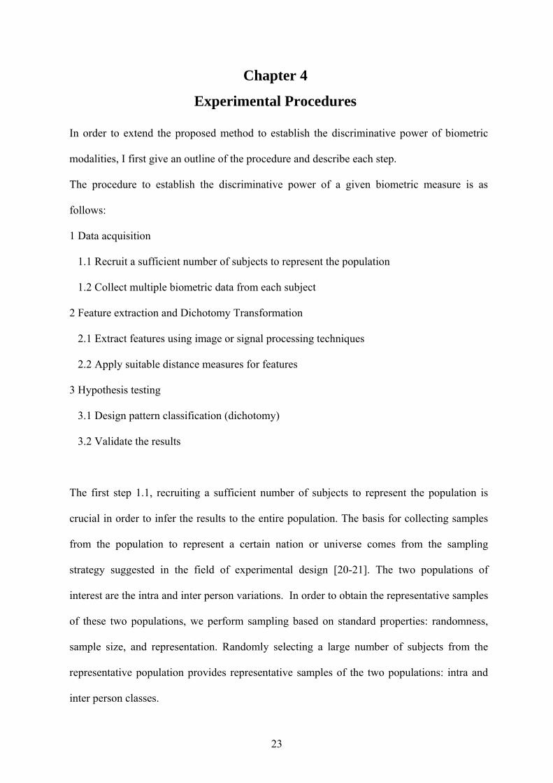
In order to extend the proposed method to establish the discriminative power of biometric

modalities, I first give an outline of the procedure and describe each step.

The procedure to establish the discriminative power of a given biometric measure is as

follows:

1 Data acquisition

1.1 Recruit a sufficient number of subjects to represent the population

1.2 Collect multiple biometric data from each subject

2 Feature extraction and Dichotomy Transformation

2.1 Extract features using image or signal processing techniques

2.2 Apply suitable distance measures for features

3 Hypothesis testing

3.1 Design pattern classification (dichotomy)

3.2 Validate the results

The first step 1.1, recruiting a sufficient number of subjects to represent the population is

crucial in order to infer the results to the entire population. The basis for collecting samples

from the population to represent a certain nation or universe comes from the sampling

strategy suggested in the field of experimental design [20-21]. The two populations of

interest are the intra and inter person variations. In order to obtain the representative samples

of these two populations, we perform sampling based on standard properties: randomness,

sample size, and representation. Randomly selecting a large number of subjects from the

representative population provides representative samples of the two populations: intra and

inter person classes.

23

Step 1.2, collecting multiple biometric data from each subject, is necessary to obtain the intra

person distance data. At least three samples per subject are recommended.

In step 2, the proposed dichotomy transformation model requires first the extraction of

features and then the application of suitable distance measures. Various image or signal

processing techniques can be used to extract features from a given modality. Depending on

the feature measurement type, suitable distance measures, e.g., Euclidean, dot-product, string

matching, histogram matching, etc, can be used to transform the feature space into the

feature-distance space.

The final step 3 is hypothesis testing. Once the two-class data, i.e., intra and inter person

distances, are computed, various pattern classifiers may be used to perform the dichotomy.

Separate intra and inter person distance data are used to validate the results. The two-class

error rate is used as the measure of individuality. Estimating the error probability is one of

the simplest problems in statistical inference [21-22] and performance evaluation [15].

The error probability estimation for the forensic and biometric data individuality problem is

depicted in Figure 7.

24

Figure 7. Error Evaluation Experimental Setup.

A large number of subjects, n, are chosen for the experiment and they provide m biometric

data each. There are two populations of interest and they are the intra person distance (or

simply intra) and inter person distance (or simply inter). A sample of intra is obtained from

pairing two biometric data samples provided by a same person. A sample of inter is obtained

from pairing biometric samples provided by two different subjects. A dichotomy classifier is

designed using the training and validation sample sets. The error probability is measured

using the testing sample sets. There are two errors for each population as discussed earlier.

The s-error is the error probability that the system classifies the two samples as a member of

intra although they were provided by two different subjects, while the d-error is the error

probability that the system classifies the two samples as a member of inter even though they

were provided by one subject. Sample error means are denoted as sX dX and for s-error

and d-error, respectively. They are often known as point estimates of the population error

means, and . sμ dμ

25

A classification system is trained using training sets intra 1 and inter 1 with two validation

sets intra 2 and inter 2. The system is tested using the remaining multiple testing sets.

and In addition to the point estimates, we are interested in confidence intervals for sμ dμ .

They are intervals within which we have reason to believe that the true population means, sμ

and , lie assuming they are normal. The formula for the α−1dμ level confidence interval

for is: sμ

[ ]

[ ] (8) )1(

1;2/1

(7) /1;2/1 for interval confidence 2

nXX

nzX

nsntX

sss

sss

−−−±≈

−−±≈

α

αμ

Because n is quite large, one can use either Student's t distribution or the normal table to

compute the confidence interval. Although the population variance is unknown [18], one

can assume that for a large n. Thus, the normal table is often used in evaluating

performance [15]. I use both, and choose the one that gives the tighter bound for the sake of

higher precision. In both cases,

2sσ

22ss s≈σ

5)1( >− pnp and thus one can use either the normal table or

the t-table.

The normality assumption on the error distribution is a sine-qua-non in the analysis. The

error probability follows a binomial distribution. A Binomial distribution gives the

probability of observing r errors in a sample of n independent instances. A discrete binomial

distribution function is then

(9) )1()!(!

!)( 4−−−

= nr pprnr

nrP

The expected, or mean value of X is

26

[ ] (10) npXE =

The variance of X is

(11) )1()( pnpXVar −=

For sufficiently large values of n the binomial distribution is closely approximated by a

Normal distribution with the same mean and variance.

),(NDerror -d and ),(NDerror -s 22

nnd

ds

sσ

μσ

μ

Most statisticians recommend using the Normal approximation only when [15]. 5)1( ≥− pnp

ss X=μ dd X=μ sXIn the final step for the hypothesis testing, claim that and where and

dX are error estimates using intra 3 and inter 3 sample sets. Given the results, we can

perform the hypotheses test on the means.

(13) :H :H

(12) :H :H2A

20

1A

10

dddd

ssss

XX

XX

≠=

≠=

μμ

μμ

I would like to validate the hypotheses using the other test sets. From intra 4 and inter 4, we

obtain new sample means, 'sX 'dXand . From the equation (8), we obtain the critical regions

for the means. If 'sX falls within the acceptance regions, accept the null hypothesis and

similarly, if

10H

'dX falls under the acceptance regions, accept the null hypothesis .

Otherwise, reject them.

20H

27

Chapter 5

Feature Extraction and Distance Measures

The dichotomy model requires the extraction of features and the use of suitable distance

measures. In this section, I review the features and distance measures previously used for iris

authentication, a subset of which I investigate and compare in this study.

First, I consider the iriscode [20], which is a 256 binary feature extracted by applying a 2D

Gabor wavelet filter. In [23], the Hamming distance in eqn (14) was used for the model in

Figure 1 (a).

yxyxyx ffffff •+•=∂''),( (14)

Second, multi-level 2D wavelet features have been widely used [24-27]. The hierarchical

wavelet transform decomposes the original iris image into a set of frequency windows having

narrower bandwidths in the lower frequency region [24]. Decomposing images with the

wavelet transform yields a multi-resolution from detailed images to approximation images in

each level. As shown in Figure 8, LH, HL, and HH represent detailed images for horizontal,

vertical, and diagonal orientation, respectively, in one-level. Sub-image LL corresponds to an

approximation image that is further decomposed, resulting in a two-level wavelet

decomposition. The result of a three-level decomposition is shown in the lower-left portion

of Figure 8.

28

IRIS part extraction

Daubechies Wavelet for an IRIS image

LL LH

HL HH

Horizontalorientation sub-image

Diagonalorientation sub-image

Verticalorientation sub-image

LH1

HL1 HH1

HH2

LH2

HH2

LL3 LH3

HH3HL3

Figure 8. Three-level wavelet transform.

L. Ma et al. tried to extract more distinctive statistical features by using a filtering process

[24]. G. Kee et al. presented a tree-structured wavelet transform in order to obtain means and

standard deviations, which are used as iris feature sets [25]. Mallat suggested that statistics

obtained from wavelet decomposition are sufficient for presenting texture difference [26].

I use the 2D Daubechies wavelet transform technique to extract features from an iris image

as folows. Each iris image is decomposed into 3 levels and each sub-image is divided into

2x2 windows, which results in 12 different sub-images. For each-sub image, mean and

variance values are calculated. As a result, 24 numeric feature values are extracted. One can

use the Euclidean distance between two vectors in eqn (15) for the Figure 1 (a) model. One

can also use the absolute vector difference measure in eqn (16) for the Figure 1 (b) model.

29

Note that the result of the eqn (15) is a scalar value whereas that of the eqn (16) is a d-

dimensional feature distance vector.

∑=

−=∂d

i

yi

xi

yx ffff1

2)(),( (15)

1 1 2 2

( , ) | |(| |, | |, , | |)

x y x y

x y x y x yd d

f f f ff f f f f f

∂ = −

= − − −L

(16)

Third, instead of extracting mean and variance values for each sub-image, I utilize 12 linear

type histograms as feature sets as previously proposed [27]. For each sub-image, the linear

type of histogram is obtained as a feature from each decomposed sub image. xif and are

ordinal histograms not simple numeric scalar values. There are numerous histogram distance

measures [29] and I consider the two popular ones: eqn (17) shows the Euclidean distance

and eqn (18) the histogram edit distance [28, 29]. Note that the histogram distance measure

is applied to each of the 12 histogram features per iris image, resulting in a 12 dimensional

feature distance vector.

yif

∑=

−=∂b

j

yji

xji

yi

xii ffff

1

2,, )(),( (17)

∑∑= =

−=∂b

j

j

k

yki

xki

yi

xii ffff

1 1,, )(),( (18)

30

Chapter 6

Binary Feature Distance Measures

In this section, I extend my study on distance measures for the binary features. I present

definitions of conventional binary feature distance measures and evaluate their performance

with proposed classificatiosn model [31].

6.1. Basic Binary Similarity Measures

Let x, y, and z be binary feature vectors of fixed length d, and let ix denote the ith feature

value which is either 0 or 1. One of the most popular measures in comparing two fixed-

length bit patterns is the Hamming distance in eqn (19), which is the count of the bits that

differ in the two patterns [33]. It is a simple geometrical distance, also known as

Manhattan or city block distance, applied to d-dimensional binary space.

1L

(19) Hamming

Hamming1

Hamming Hamming

Hamming1

( , )

( , )

( , ) ( , )

( , )

1 if where

0 otherwise

t t

d

i ii

t t

d

ii

i ii

D x y x y x y

D x y x y

S x y d D x y x y x

S x y s

x ys

=

=

= +

= −

= − = +

=

=⎧= ⎨⎩

∑

∑

y

tx y xThe term denotes the positive matches, i.e., the number of 1 bits that match between

and . The term y tyx is the negative matches, i.e., the number of 0 matching bits. The terms

tx y tx y and denote the number of bit mismatches – the first where pattern x has 1 and

pattern y has 0, and the second where pattern x has 0 and pattern y has 1.

31

Fact 1. The Hamming distance has been shown to be metric [14].

While the Hamming distance is the number of bits differing in the two patterns, the

Hamming similarity is the number of identical bits in the two patterns. Sokal and Michener

normalized the Hamming similarity as in eqn (20) [34], and an alternative normalized

Hamming similarity is given by Rogers and Tanimoto in eqn (21) [35].

Sokal-Michener ( , )t tx y x yS x y

d+

= (20)

Rogers-Tanimoto ( , )2 2

t t

t t t t

x y x yS x yx y x y x y x

+=

+ + +(21)

y

tx yThe term is the inner product of two vectors, which yields a scalar, and it is sometimes

called the scalar product or dot product. It can be converted to a distance by subtracting it

from d, and this distance is clearly non-metric because of the reflexivity violation;

ifinner-product ( , ) 0D x y = x y= and | | | |x y d= = and , otherwise. inner-product ( , ) 0D x y >

Fact 2. Nonnegativity, symmetry, and triangle inequality are trivial and preserved in the

inner product [36].

(22) inner-product

inner-product1

( , )

( , )

1 if 1 where

0 otherwise

t

d

ii

i ii

S x y x y

S x y s

x ys

=

=

=

= =⎧= ⎨⎩

∑

32

A normalized inner product is given in eqn (23) [14] and various alternative normalizations

in eqns (24~27) [37-39, 42].

normalized-inner-product ( , )t t

t t

x y x yS x yx y x xy y

= = (23)

Russell-Rao ( , )tx yS x yd

= (24)

Jaccard-Needham ( , )t

tt t

x yS x yyx y x y x

=+ +

(25)

Dice ( , )2

t

tt t

x yS x yyx y x y x

=+ +

(26)

Kulzinsky ( , )t

tt

x yS x yyx y x

=+

(27)

The Jaccard, Dice, and Kulzinsky similarity measures differ in their ranges: the Jaccard

measure ranges from 0 to 1, the Dice measure from 0 to ½, and the Kulzinsky measure from

0 to ∞. Eqns (25~27) can be generalized to eqn (28) which for 0σ = becomes the Kulzinsky

coefficient, for the Jaccard coefficient, and for the Dice coefficient. 1σ = 2σ =

Generalized Jaccard ( , )t

tt t

x yS x yyx y x y xσ

=+ +

(28)

Another popular distance measure between binary feature vectors is the Tanimoto metric

defined in eqn (29) [14] where xn and are the numbers of 1 bits in x and y, respectively,

and

yn

tx y,x yn is .

33

(29) ,

,

2( , )

x y x yTanimoto

x y x y

t t

t t t

n n nD x y

n n n

x y x yx y x y x y

+ −=

+ −

+=

+ +

The Tanimoto coefficient [14], defined in eqn (30), is another variation of the normalized

inner product which is frequently encountered in the fields of information retrieval and

biological taxonomy.

( , )t

Tanimoto t t t

x yS x yx x y y x y

=+ −

(30)

Most similarity measures are variations either of Hamming or of the inner-product. Generally,

the former ones treat the presence, tx y , and the absence, tx y , of features equally while the

later take only the presence, tx y , into account and exclude tx y . The decision to include or

exclude the tx y term is a difficult and contentious one [42, 43]. Prior to 1950 when the

Hamming distance was introduced, the use of inner-product based similarity coefficients

flourished. Sokal and Michener made a good argument to include the negative matches [34,

42, 43] but they used equal weights for both positive and negative matches.

tyx term, eqn (31), where Hence, we propose a new measure with variable credit for the σ

is the contribution factor, and 0 σ≤ ∞ . We call it the azzoo similarity measure because we

can alter the credit for the zero-zero matches relative to that for the one-one matches (azzoo =

alter zero zero one one).s

34

(31)

1 1

1

( , )

(1 )(1 )

( , )

1 if 1 where if 0

0 otherwise

t tazzoo

d d

i i i ii i

d

azzoo ii

i i

i i

S x y x y x y

x y x y

S x y s

x ys x y

σ

σ

σ

= =

=

= +

= + − −

=

i

= =⎧⎪= = =⎨⎪⎩

∑ ∑

∑

, becomes the inner product, and for azzooSNote that for 0σ = 1σ = , the Hamming similarity

measure. Although requires finding the optimal azzooS σ factor, the experimental results in

later sections show that it outperforms both the Hamming and inner-product similarity

measures.

00 11S −Originally, the half-credit similarity, was used in an offline handwriting recognition

system [44] and it is the same as with azzooS 0.5σ = . It gives full credit to features present in

both patterns, tx y , half credit to those not present in either pattern, tyx , and no credit to

those present in only one of the patterns, tx y tx y and , as defined in eqn (32) [44, 45, 46]

and here we generalized the half-credit similarity to . azzooS

The range of is

00 11( , )2

tt x yS x y x y− = + (32)

[ ]0,dazzooS if 0 1σ≤ ≤ and [ ]0, dσ if . Assuming 0 11σ > σ≤ ≤ , can

be converted to a distance measure for metric property testing, eqn (33).

azzooS

( )( , ) ( , ) t tazzoo azzooD x y d S x y d x y x yσ= − = − + (33)

35

Nonnegativity and symmetry are trivial and preserved. Reflexivity is violated, however, because

iff( , ) 0azzooD x y = and | | | |x y x y= = d= and ( , ) 0azzooD x y ≠ otherwise. Similarly,

if ( , )azzooS x y = d x y= and| | | |x y d= = and 00 11( , )d S x y dσ −≤ < x y= and | |x d<if .

Theorem 1. The triangle inequality property is valid for , i.e., ( , )azzooD x y

( , ) ( , ) ( , )azzoo azzoo azzooD x y D y z D x z+ ≥ .

Proof

by Fact 1 line 1( )+ ( ) ( ) by Fact 2 line 2

Now, evaluate ( , ) ( , ) ( , ).

t t t

t t t t t t

azzoo azzoo azzoo

x y y z x zd x y x y d y z y z d x z x z

D x y D y z D x z

+ ≥

− + − + ≥ − ++ ≥

( )+ ( ) ( )( )+ ( ) (1 ) (1 )

( ) (1 )Hence, the theorem is true by line 1 and line 2

t t t t t t

t t t t t t

t t t

d x y x y d y z y z d x z x zd x y x y d y z y z x y y z

d x z x z x z

σ σ σ

σ σ

σ

− + − + ≥ − +

− + − + + − + −

≥ − + + −

inner-product inner-product( , ) ( , ) ( , )t tazzooS x y x y x y S x y S x yσ σ= + = +Similarly, since , the

properties of the azzoo similarity measure are similar to those of the inner-product measure.

Other popular similarity measures utilize coefficients of correlation and have been used

frequently in both psychology and ecology studies [42]. The correlation similarity measure is

given in eqn (34) and Yule and Kendall [40] suggested a similar coefficient given in eqn (35).

correlation)( )( )( )(

t t t t

t t t t tt t t

x y x y x y x ySy x y x y x y x yx y x y x y x

× − ×=

+ ++ + (34)

Yule

t t t t

t t t t

x y x y x y x ySx y x y x y x y

× − ×=

× + × (35)

While Hamming based similarity measures are additive forms of the positive and negative

matches, the correlation based measures are multiplicative forms. Nonetheless, contribution

36

factors of positive and negative matches are considered equally important in correlation

based similarity measures as well as Hamming based ones.

1908

Jaccard

21st Century

azzoo

1950

Hamming

1958

Sokal & Michener

1960

Roger & Tanimot

o

1945

Dice

1940

Russell & Rao

1927

Kulzinsky

1936 1911

Tanimoto

Correlation Yule

(inner-product based)

(correlation based)

(Hamming based)

Figure 9. A chronological table for binary vector similarity measures.

Historically, all the measures enumerated above have had great value in their respective

fields. Figure 9 shows a chronological table for binary feature vector similarity measures in

which these conventional measures are categorized into three major groups: inner-product,

Hamming, and correlation based groups.

6.2. Binary Similarity Measures with Weights

To further improve their discrimination capability, weights can be applied to distance or

similarity measures [44] and optimized using techniques such as genetic algorithms [47, 48].

When features have numeric values, a scaling problem arises. In order to mitigate this

problem, one can combine the nonlinear accuracy weighting with the Minkowski distance

concept as shown in eqn (36) where is the probability of being correct when only

feature i is used [41, 42].

( / )P C i

37

weighted Minkowski1

( / )d

rai i

iD P C i

=

x y⎡ ⎤= −⎣ ⎦∑ (36)

When features are binary, one can still generalize eqn (36) to eqn (37) by setting and

.

1r =

( / )aiP C i w=

(37) weighted-Hamming

1

weighted-Hamming1

( , )

( , ) ( )

d

i i iid

i i i i ii

D x y w x

S x y w x y x y

=

=

= −

= +

∑

∑

y

w x y

The weighted Hamming distance has been applied to numerous applications such as image

template matching [49, 50] and object recognition [50]. The weighted Hamming distance

provides an improvement over the simple Hamming distance for discriminating between

similar images [49, 50]. This distance measure gives greater importance to error pixels which

appear in close proximity to other error pixels. Error pixels which appear close together tend

to correspond to structurally meaningful features. In [51], a slightly different weighted

Hamming distance was introduced to optimize the distance measure for object detection by

adding a null weight, . Similarly, the inner product similarity measure can be optimized

by applying weights as shown in eqn (38).

0w

weighted-inner-product1

( , )d

i i ii

S x y=

= ∑ (38)

Here, we claim that the performance can be further improved by optimizing the similarity

measure rather than distance measure. Since the Hamming distance is the number of

mismatches, the weights are applied to the mismatched bits, whereas in a similarity measure

38

the weights are applied to the matching bits. As discussed in the earlier section, there are two

kinds of matches: positive and negative matches. Although the Hamming similarity can be

improved by applying the equal weights are applied to both positive and negative matches,

we claim that if different weights are applied, the performance is further improved, and the

proposed weighted 00-11 similarity measure is given in eqn (39).

00 111 1

( , )d d

weighed i i i i i ii i

S x y w x y w− − ⊕ Θ= =

= +∑ ∑ x y(39)

Note that if w and are identical, wΘ 00 11 weighted-hammingweighedS S− − = 0wΘ = and if ,

.

⊕

00 11 weighted-inner-productweighedS S− − =

There are twice as many coefficients to optimize in this new similarity measure than in the

weighted Hamming or inner product similarity measures. This is a multi-dimensional, space

optimization problem, and one can use a genetic algorithm to determine the weights from

training data. A genetic algorithm can be a general optimization method that searches a large

space of candidate objects to find one that performs near optimal according to the fitness

function [46, 47]. Genetic algorithms offer a number of advantages: they search from a set of

solutions rather than from a single one, they are not derivative-based, and they explore and

exploit the parameter space. For the weight adaptive model, we create a numerical

optimization model that depends on a set of weights.

6.3. Evaluation for the Binary Feature Distance Measures

The iris biometric verification models were trained on 500 distance or similarity values

obtained from the intra- and inter-class sets. These scalar values form distributions and the

39

mean and variance can be computed for each distribution. Assuming normal distributions,

one can easily find the Bayes decision threshold. For testing, each scalar distance value is

classified into the intra or inter person class by comparing to the threshold value. Figure 10

depicts the intra and inter similarity distributions using various similarity measures and Table

1 shows the comparative results of the overall performances. Finally, Figure 11 shows the

performance as a function of the contribution factor, σ , and highlights the relative

performance of the inner product, Hamming, and azzoo measures. The with azzooS

1.175σ = yields the best performance.

40

41

Figure 10. Intra and inter distance distributions for the various similarity measures.

Table 1. Performance evaluation of the similarity measures on the iris database. Data 1 Data 2 Data 3 Data 4 Total

Method FAR FRR Rate FAR FRR Rate FAR FRR Rate FAR FRR Rate Rateazzoo 5.0 4.4 95.3 6.4 3.2 95.2 7.6 3.2 94.6 4.4 3.8 95.9 95. normalized I.P. 4.8 4.8 95.2 6.0 4.4 94.8 7.4 3.6 94.5 5.0 4.4 95.3 95. SokalMichener 5.0 4.8 95.1 6.4 3.6 95.0 7.8 3.2 94.5 4.6 3.8 95.8 95. RogersTanmoto 5.0 4.8 95.1 6.4 3.6 95.0 7.8 3.2 94.5 4.6 3.8 95.8 95. RussellRao 12.8 12.2 87.5 11.8 10.4 88.9 11.4 8.6 90.0 11.2 10.4 89.2 88. JaccardNeedham 4.8 4.8 95.2 6.2 4.2 94.8 7.4 3.6 94.5 5.0 4.0 95.5 95. Dice 4.8 4.8 95.2 6.0 4.2 94.9 7.4 3.6 94.5 5.0 4.4 95.3 95. Kulzinsky 6.8 3.8 94.7 7.4 3.0 94.8 9.0 2.6 94.2 6.4 3.4 95.1 94. Tanimoto 4.8 4.8 95.2 6.2 4.2 94.8 7.4 3.6 94.5 5.0 4.0 95.5 95. correlation 5.4 4.6 95.0 6.4 3.8 94.9 7.8 3.2 94.5 4.2 3.6 96.1 95. Yule 4.8 4.8 95.2 5.6 4.8 94.8 7.8 3.0 94.6 4.0 3.8 96.1 95.

30119007012

Figure 11. Performance vs. the contribution factor σ .

42

Chapter 7

Comparative Experimental Results

In this section, I compare the experimental results obtained by using several classifiers with a

variety of different features and distance measures. From the iris biometric image database

[25], I selected 10 left bare eye samples of 52 subjects.

IRIS database[25] consists of subject demographic data and features obtained from an IRIS

sample. . From 60 subjects, 800 IRIS images are taken. Each subject provided 10 exemplars.

Thus, the IRIS database consists of two entities: subject data and IRIS feature data. Figure 12.

shows a few exemplars from the IRIS database. Age range is from 19 to 36. Iris images

distinguish left or right eyes and whether the subject wears glasses or lens. For the

experiment, 10 left bare eye samples of 52 subjects are used [27].

Bare eyes With Glasses With Lens

Figure 12. Samples from the IRIS database.

In order to test the described models, two sets of samples are required: intra-class distance

and inter-class distance sets. The intra-class distance sample is acquired by randomly

43

selecting two iris data from the same subject while the inter-class distance sample is obtained

by randomly selecting two iris data from two different subjects. I prepared three sets of inter

and intra distance data for training and three independent ones for testing, each of size 1000

(500 intra-class and 500 inter-class pairs).

Table 2. Eleven different models

Features Distance Classifier

1 Iriscode (Binary) Hamming eq (7) Bayes decision

Wavelet means & variances 2 Euclidean eq (8) Bayes decision

Wavelet means & variances 3 Vector difference eq (9) Nearest Neighbor

Wavelet means & variances 4 Vector difference eq (9) ANN

Wavelet means & variances 5 Vector difference eq (9) SVM

6 Wavelet histo Euclid eq (10) Nearest Neighbor

7 Wavelet histo Euclid eq (10) ANN

8 Wavelet histo Euclid eq (10) SVM

9 Wavelet histo Edit dist eq (11) Nearest Neighbor

10 Wavelet histo Edit dist eq (11) ANN

11 Wavelet histo Edit dist eq (11) SVM

As shown in Table 2, I examined eleven different models. Models 1 and 2 use the parametric

verification model of Figure 1 (a), and the remaining models use the dichotomy

transformation model of Figure 1 (b).

The parametric method models 1 and 2 were trained on 500 scalar distance values obtained

from the intra- and inter-class sets. These scalar distance values form distributions and the

44

mean and variance can be computed for each distribution. Assuming normal distributions,

one can easily find the Bayes decision threshold. For testing, each scalar distance value is

classified into the intra- or inter-distance class by comparing to the threshold value as

depicted in Figure 3 (a).

Table 3. Parametric model evaluation results:

1000 sample pairs per test.

Model Sets FRR FAR Performance Training 19.0% 21.5% 79.8%

Test 1 10.2% 4.6% 92.6% Test 2 12.0% 3.2% 92.4%

1 iriscode + Hamming eqn (7)

Test 3 10.4% 3.2% 93.2% Training 13.5% 23.2% 81.7% Test 1 4.2% 25.6% 85.1% Test 2 5.6% 23% 85.7%

2 Wavelet means & variances + Euclidean eqn (8)

Test 3 4.6% 24.2% 85.6%

Table 3 shows the error rates and overall performance values for models 1 and 2. Two

observations can be drawn from these results. First, the results of the traditional parametric

model using the scalar distance measure in Figure 2 (a) are disappointing compared to those

of the other model in Figure 2 (b). The reason is that multivariate distance analysis is clearly

better than a single scalar distance analysis. The other observation is that the FRR in the

testing sets are much smaller than those in the training set, suggesting that the two

distributions are not normal.

Models 3-11 used the dichotomy transformation to obtain 500 samples of d-dimensional

feature distance vectors for intra- and inter-class sets. Regardless of the types of features, the

feature distance vectors are all numeric values when proper distance measures are applied.

Thus, the feature distance vectors become inputs to the dichotomizer as shown in Figure 1 (b).

45

I tested three well-known classifiers [14] as the dichotomizer: nearest neighbor, artificial

neural network (ANN), and support vector machine (SVM).

I selected the artificial neural network for a dichotomizer because it is equivalent to

multivariate statistical analysis. There is a wealth of literature regarding a close relationship

between neural networks and the techniques of statistical analysis, especially multivariate

statistical analysis, which involves many variables [14, 30]. I selected the support vector

machine because it has gained considerable popularity recently and has become state-of-the-

art [32].

Table 4. Dichotomy model performance results:

1000 independent sample pairs per test.

Wavelet means & variances (Models

3-5)

Wavelet histogram + eqn (10)

Wavelet histograms + eqn (11)

(Models 6-8)

(Models 9-11)

Test 1 90.5 81.0 89.9 Test 2 90.8 80.6 92.6 Nearest

Neighbor Test 3 91.0 81.3 92.0 Training 95.8 90.9 99.2 Test 1 94.8 82.4 96.1 Artificial

Test 2 96.7 83.8 96.9 Neural Network

Test 3 95.6 82.5 96.7 98.8 Training 97.6 88.9

Test 1 96.2 85.7 97.9 Support

Test 2 97.5 86.3 98.5 Vector Machine

97.9 Test 3 96.7 86.8

Table 4 shows performances of models 3-11. In general, support vector machines outperform

artificial neural networks which, in turn, outperform nearest neighbor classifiers. The best

46

performing SVM model was the one using the 2D three-level wavelet histogram features

with the histogram edit distance in eqn (11).

47

Chapter 8

Conclusions

In this paper, I considered the problem of establishing iris individuality. I first argued that

the quantitative error rate measure for the biometric identification model is not appropriate

for the measure of establishing biometric individuality since the error rate cannot be inferable

to the entire population. I also argued that FRR and FAR from the biometric verification

model are adequate measures that are inferable to the entire population. I performed the

evaluation of conventional binary feature distance measures. I examined eleven biometric

verification models for the problem of establishing iris individuality.

To establish the discriminative power of the individuality of the iris biometric, I used a 52-

subject iris image database. I transformed the many-class problem into a dichotomy problem

by using distances between two samples of the same class and between two samples of

different classes. I examined eleven ways of implementing a dichotomy model by selecting

different combinations of features, distance measures, and classifiers. Of these eleven models,

I found that the combination of multi-level 2D wavelet features, histogram distances, and a

support vector machine classifier yielded the best overall correctness of 98%.

48

References

[1] United States Supreme Court ruling, “Daubert vs. Merrell Dow Pharmaceuticals,” 509 U.S.

579, 1993.

[2] R. M. Bolle, J. H. Connell, S. Pankanti, N. K. Ratha, and A. W. Senior, “Guide to

Biometrics,” Springer Professional Computing, ISBN 0-387-40089-3, 2003

[3] S. Cha and S. N. Srihari, “Writer Identification: Statistical Analysis and Dichotomizer,” in

Proceedings of SPR and SSPR 2000 Alicante, Spain 2000, LNCS - Advances in Pattern

Recognition, vol. 1876, p 123-132

[4] S.-H. Cha, “Use of Distance Measures in Handwriting Analysis,” PhD dissertation, SUNY at

buffalo, CSE, March, 2001.

[5] S. N. Srihari, S.-H. Cha, H. Arora, and S. Lee, “Individuality of Handwriting,” Journal of

Forensic Sciences, vol. 47, no. 4, pp 856-872, 2002.

[6] D. Stoney and J. Thornton, “A Critical Analysis of Quantitative Fingerprint Individuality

Models,” Journal of Forensic Sciences, vol. 31, no. 4, pp. 1187-1216, 1986.

[7] M. Kam, J. Wetstein, and R. Conn, “Proficiency of Professional Document Examiners in

Writer Identification,” Jouranl of Forensic Sciences, vol 39, pp. 5-14, January 1994.

[8] M. Kam, B. Fielding, and R. Conn, “Writer Identification by Professional Document

Examiners,” Jouranl of Forensic Sciences, vol 42, pp. 778-786, January 1997.

[9] C.M. Greening and V.K. Sagar, “Image Processing and Pattern Recognition Framework for

Forensic Document Analysis,” in IEEE Annual International Carnahan Conference on

Security Technology, pp. 295-300, IEEE, 1995.

[10] G. Holcombe, G. Leedham, and V. Sagar, “Image Processing Tools for the Interactive

Forensic Examination of Questioned Documents,” in IEE Conference Publication, no. 408,

pp. 225-228, 1995.

49

[11] C.M. Greening, V. K. Sagar, and C. G. Leedham, “Handwriting Identification using Global

and Local Features for Forensic Purposes,” in IEE Conference Publication, no. 408, pp. 272-

278, 1995.

[12] R. Plamondon and G. Lorette, “Automatic Signature Verification and Writer Identification-

the State of the Art,” Pattern Recognition, vol. 22, no. 2, pp. 107-131, 1989.

[13] S. Pankanti, S. Prabhakar, and A. K. Jain, “On the Individuality of Fingerprints,” IEEE

Transactions on Pattern Analysis and Machine Intelligence, vol. 24, no. 8, pp. 1010-1025,

2002.

[14] R. O. Duda, P.E. Hart, and D. G. Stork, Pattern Classification, John Wiley & Sons, Inc. 2nd

ed., 2000.

[15] T. Mitchell, Machine Learning, McGraw Hill, 1997.

[16] H. Liu and H. Motoda, “Feature Selection for Knowledge Discovery and Data Mining”,

Kluwer Academic Publishers, 1998.

[17] S.-H. Cha and S. N. Srihari, “Multiple Feature Integration for Writer Verification,” in

Proceedings of 7th IWFHR 2000, pp. 333-342, September 2000.

[18] S. Yoon, S. Choi, S. Cha, Y. Lee, and C. C. Tappert, “On the Individuality of the Iris

Biometric” in International Journal on Graphics, Vision and Image Processing, Vol. 5,

2005.

[19] M. Gibbons, S. Yoon, S. Cha, and C. C. Tappert, “Biometric Identification Generalizability”

in Proceedings of Audio- and Video-based Biometric Person Authentication, Rye Brook, NY,

July, 2005.

[20] S. L. Lohr, Sampling: Design and Analysis, Duxbury Press, Pacific Grove, CA, 1999.

[21] Ol J. Dunn and V. A. Clark, Applied Statistics: Analysis of Variance and Regression, John

wiley & Sons, 2nd ed.m 1987.

[22] N. A. Weiss, Introduction Statistics, Addison-Wesley, 5th ed., 1999.

50

[23] J.G. Daugman, “High confidence visual recognition of persons by a test of statistical

independence,” IEEE Transactions on Pattern Analysis and Machine Intelligence,

15(11),:1148-1161 November, 1993.

[24] L. Ma, T. Tan, Y. Wang, and D. Zhang, “Personal Identification Based on Iris Txture

Analysis”, IEEE Transactions on Pattern Analysis and Machine Intelligence, Vol. 25, No,

12, 2003.

[25] G. Kee, Y. Byun, K, Lee and Y. Lee, “Improved Techniques for an Iris Recognition System

with High Performance”, Lecture Notes Artificial Intelligence, 2001.

[26] Mallat, S.G., “A theory for Multiresolution Signal Decomposition: The Wavelet

Representation”, IEEE Tans. Pattern Recognition and Machine Intelligence, 11(4), pp. 674-

693, 1989.

[27] S. Choi, S. Yoon, S._H. Cha, and C. C. Tappert, “Use of Histogram Distances in Iris

Authentication,” in Proceedings of International Conference on Machine Learning; Models,

Technologies and Applications, Las Vegas, Jun 21-24, 2004.

[28] S. Cha and S. N. Srihari, “On Measuring the Distance between Histograms”, in Pattern

Recognition, Vol 35/6, pp 1355-1370, June 2002.

[29] S. Cha, “Fast Image Template and Dictionary Matching Algorithms”, in Proceedings of

ACCV '98, Hongkong, LNCS -Computer Vision, vol. 1351, p370-377, Springer yr. 1997.

[30] V. Cherkassky, J. H. friedman, and H. Wechsler, From Statistics to Neural Networks: Theory

and Pattern Recognition Applications, Springer, NATO ASI ed., 1994.

[31] S. Cha, S. Yoon, and C. C. Tappert, “Enhancing Binary Feature Vector Similarity

Measures”, CSIS Technical Reports, n 210, , Jan 2005.

[32] Edgar E Osuna, Robert Freund and Federico Girosi. Support Vector Machines: Training and

Applications. MIT Artificial Intelligence Laboratory and Center for Biological and

51

Computational Learning Department of Brain and Cognitive Sciences. A.I. Memo No 1602,

C.B.C.L. Paper No 144, 1997.

[33] R. V. Hamming, “Error detecting and error correcting codes”, Bell Sys. Tech. Journal,

29:147-160, 1950.

[34] R. R. Sokal and C. D. Michener, “A statistical method for evaluating systematic

relationships”, University of Kansas Scientific Bulletin 38, 1409-1438, 1958.

[35] D. J. Rogers and T. T. Tanimoto, “A computer program for classifying plants”, Science,

132:1115-1118, 1960.

An Introduction to Hilbert Spaces and the Theory of Spectral Multiplicity[36] Paul R. Halmos, ,

Chelsea Plublishing, 2nd ed, 1957.

[37] P. F. Russell and T. R. Rao, “On habitat and association of species of anopheline larvae in

south-eastern Madras”, J. Malar. Inst. India, 3:153-178, 1940.

[38] P. Jaccard, “Nouvelles recherches sur la distribution florale”, Bulletin de la Societe Vaudoise

de Science Naturelle, 44, 223-270, 1908.

[39] L. R. Dice, “Measures of the amount of ecologic association between species”, Ecology,

26:297-302, 1945.

[40] G. U. Yule and M.G.Kendall, An Introduction to the Theory of Statistics, 14th ed. Hafner,

New York, pp701, 1950.

[41] C. Gose, R. Johnsonbaugh, and S. Jost, Pattern Recognition and Image Analysis, Prentice

Hall, Inc., p 172, 1996.

[42] P. H. A. Sneath and R. R. Sokal, Numerical Taxonomy, London: Freeman, 1973.

[43] G. Dunn and B. S. Everitt, An introduction to mathematical taxonomy, Cambridge University

Press 1982.

52

[44] J. T. Favata and G. Srikantan, “A multiple feature/resolution approach to handprinted digit

and character recognition”, International Journal of Imaging Systems and Technology, pp.

7:304–311, 1996.

[45] S.-H. Cha and S. N. Srihari, “A fast nearest neighbour search algorithm by filtration”,

Pattern Recognition 35, P 515-525, 2000.

[46] S.-H. Cha and C. C. Tappert , “Optimizing Binary Feature Vector Similarity Measure using

Genetic Algorithm”, ICDAR, Edinburgh, Scotland, 2003.

[47] M. Mitchell, An introduction to genetic algorithms, Cambridge, MA: MIT Press, 1996.

[48] L. Davis, Handbook of genetic algorithms. New York: Van Nostrand Reinhold, 1991.

[49] W. Pratt, P. Capitant, W. Chen, E. Hamilton, and R. Willis, “Combining symbol matching

facsimile data compression system”, in Proceedings of the IEEE, 68:786-796, 1980.

[50] I. Witten, A. Moffat, and T. Bell, Managing Gigabytes: Compressing and Indexing

Documents and Images, Van Nostrand Reinhold, 1994.

[51] S. Mahamud and M. Hebert, “The Optimal Distance Measure for Object Detection”,

IEEE Computer Vision and Pattern Recognition, Wisconsin, p 248-256, 2003.

53