A study of the Delta Normal Method of Measuring VaR · PDF fileA study of the Delta Normal Method of Measuring VaR A Thesis Submitted to the Faculty ... Rajesh Kondapaneni _____ Date:

A study of the Delta Normal Method of Measuring VaR

A Thesis

Submitted to the Faculty

of the

WORCESTER POLYTECHNIC INSTITUTE

In partial fulfillment of the requirements for the

Professional Masters Degree in Financial Mathematics

By

Rajesh Kondapaneni

______________________________

Date: May 5, 2005

APPROVED:

_____________________________________________

Professor Arthur C. Heinricher, Thesis Advisor

_____________________________________________

Professor Bogdan Vernescu, Head, Mathematical Sciences Department

Abstract

This thesis describes the Delta-Normal method of computing Value-at-Risk. The

advantages and disadvantages of the Delta-Normal method compared to the Historical

and Monte Carlo method of computing Value-at-Risk are discussed. The Delta-Normal

method of computing Value-at-Risk is compared with the Historical Simulation method

of Value-at-Risk using an implementation of portfolio consisting of ten stocks for 400

time intervals.

Based on the normality of the distribution of the portfolio risk factors, Delta-Normal

would be suitable if the distribution is normal and Historical Simulation method of

calculating Value-at-Risk would be ideally suited if the distribution is non-normal.

i

Acknowledgements

I would like to thank the faculty and students of the Mathematics Department for

their help and support during my tenure here at WPI. I would especially like to thank

Professor Heinricher for his patience and guidance in helping me with this project. I am

very thankful to Professor Heinricher for his knowledge and critical guidance. I am

thankful to Professor Domokos Vermes for his encouragement and support during the

various stages of my graduate study.

I would also like to thank Professor Bogdan Vernescu, Professor Joseph Petrucelli

and other members of the Graduate Committee for providing me with an assistantship to

pursue my master’s degree. I want to thank my family and friends who have always

encouraged me.

ii

Table of Contents

Abstract…………….………………………………………………………………………i Acknowledgements…………….…………………………………………………….........ii

1 Introduction and Background…………....................................................................1 1.1 Mean Variance Analysis................................................................................................1 1.2 Alternate Risk Measures……………..………………………………………………..2 1.3 Need for Value-at-Risk……………..………………………………………………....3 1.4 Criticism of Value-at-Risk…………….………………………………………………4 1.5 Overview of the Report……………..…………………………………………………4

2 Value-at-Risk Definition……………..........................................................................6

2.1 Computation of Value-at-Risk ………………….………………….………………11

3 Value-at-Risk Methods………………………………………………………….….15

3.1 Historical Simulation Method:...………………………...…………………………...15 3.1.1 Advantages………………………………………….……………………………15 3.1.2 Disadvantages........................................................................................................16

3.2 Monte Carlo Simulation Method:...…..…...…………………………………………16 3.2.1 Advantages………………….................................................................................16 3.2.2 Disadvantages……………………………………………………………………17

3.3 Delta-Normal Method:………………...……………………………………………..17 3.3.1 Advantages………………….……………………………………………………18 3.3.2 Disadvantages……………………………………………………………………18 3.3.3 Implementation...……………...……………………………………...…………19 3.3.4 Proof of VaR Formula using VaR Definition……………....................................21 3.3.5 Optimization………………………......................................................................24

4 Results and Analysis: …………………………………………...………………….26 4.1 Implementation of Delta-Normal………….………………………………………....26 4.2 Implementation of Historical Simulation…………………………………………….28 4.3 Results..…………………………………………………………………………..…..29 4.4 Analysis………………………………………………………………………………31

5 Conclusion…………………………………………………………......................…38

References……………………………………………………………………………….39 Appendix A: Matlab Code……………….…………………………………………….40 Appendix B: Efficient Frontier and Portfolio Bar Allocation Charts……………....44 Appendix C. SaS Results I…………………………………………………………….47

Appendix D. SaS Results II…………………………………………………………….77

iii

1. Introduction & Background

Risk measurement is a classical problem in finance. Harry Markowitz’s work [2]

was the first that gave a clear mathematical definition to “risk” in portfolio analysis.

Markowitz did not actually use the word “risk” in his original paper but he only said that

the variance (or standard deviation) in return on the portfolio is the quantity that an

investor would like to minimize while maximizing the return on the portfolio. The

intuitive definition of risk is the probability of suffering harm or loss. Any mathematical

definition of risk must capture and quantify the idea that return is a random variable and

risk is the probability or possibility of loss (References [4, 5, and 6]).

1.1 Mean Variance Analysis

Given a portfolio of assets, the investor chooses to invest a fraction of total

wealth in each of assets with (random) return . The expected return on the

portfolio is the weighted average of the individual expected returns:

N

ih N iR

[ ] [ ] ∑∑==

====N

iii

N

iiipP hREhRE

11µµ µTh .

The risk associated with the portfolio is the variance (or standard deviation) of the return

on the portfolio (see [2]) :

[ ] === ∑∑==

N

ijiji

N

jpP hhRVar

11

2 σσ ChhT

Where C is the x covariance matrix with entries N N

[ ]))(( jjiiij RRE µµσ −−=

1

To say that the return on a portfolio is a random variable means that the (future) return is

not known in advance but the analyst has some way of modeling the distribution of

possible returns and their associated probabilities.

1.2 Alternate Risk Measures

In some applications, variance may not be the best measure of risk for a stock or

portfolio. There are other risk measures that are easier to interpret and easier to explain to

a client. These other risk measures have been developed and applied (see, for example,

Chapter 3 in [3]). These risk measures include:

• Semivariance (also called downside risk or downside variance);

• Target semivariance;

• Shortfall probability;

• Value at Risk.

Semivariance simply assumes that the investor only cares about large shifts in the

price of a stock if the large shifts are below the mean. If the distribution is symmetric,

then semivariance is simply a multiple of variance and so no new information is

recorded. If the distribution is not symmetric, then semivariance does capture useful

information which variance would miss.

Target semivariance goes one step further and records only drops in price larger

than a certain (target) threshold. It is a generalization of semivariance that focuses on

returns below a target, such as zero or the risk free rate instead of just below the mean.

Shortfall probability records the part of the distribution in returns that is below a

certain threshold. It answers the question “What is the probability that returns will be

below X ?” for a specified X .

2

One of the most used alternative risk measure is Value at Risk (VaR). It records

the actual loss that would occur if the returns were below a certain probability threshold

of the distribution. Note that, as with the semivariance, when the distribution of returns is

normal, then the value at risk is a multiple of the variance. Even in this situation where

the two measures really provide the same information, some clients will demand a report

of value at risk for a portfolio.

1.3 Need for Value-at-Risk

The concept and use of Value-at-Risk is recent. Value-at-Risk was first used by

major financial firms in the late 1980’s to measure the risk of their trading portfolios.

Since that time, the use of Value-at-Risk has exploded.

Value-at-Risk is now a widely used quantitative tool to measure market risk.

“VaR answers the question: how much can one lose with X % probability over a pre-set

horizon” [8]. More precisely VaR is an amount (say V dollars), where the probability of

losing more than V dollars is over some future time interval, T days. Value at Risk

measures the amount of risk in dollars. Investors can then decide whether they feel

comfortable with this level of risk.

∗p

Value-at-Risk asks the simple question “How bad can things get?” All managers

would like this question to be answered. Value-at-Risk has become widely used by

corporate treasurers and fund managers as well as by financial institutions. Value-at-Risk

is used by bank regulators in determining how much capital a bank should possess to

reflect the market risks it is bearing [8]. Today, many banks, brokerage firms and

investment funds use similar methods to gauge their financial risk. A 1995 Institutional

Investor survey found that 32% of all firms use VaR as a measure of market risk, and

3

60% of pension funds responding to a survey by the New York University Stern School

of Business reported using VaR (chapter 9, [9] ) .

1.4 Criticism of Value-at-Risk

The widespread adoption of VaR has been accompanied by frequent criticism of

VaR as a measure of risk. Any attempt to summarize a distribution in a single number is

open to criticism, but VaR has a particular deficiency. Combining two portfolios into a

single portfolio may result in a VaR that is larger than the sum of the VaRs for the two

original portfolios. This fact contradicts the idea that diversification reduces the risk [7].

VaR assumes that the sigma and covariance matrix do not change. VaR fails when

you need it the most i.e, it is uninformative about extreme tails. One good example is

Long Term Capital Management (LTCM). Due to its shortcomings, it should not be used

as a standalone risk measure, but one of many risk measures to be considered in firm

wide risk management

1.5 Overview of this Report

Our goal is to study in detail the Delta-Normal Method of computing Value-at-

Risk. This project report focuses on computing Value-at-Risk for a portfolio of ten stocks

using the Delta-Normal Method and the Historical Simulation Method. The next section

gives the definition of Value-at-Risk and the steps involved in computing it. We then

give an overview of the different methods used to compute Value-at-Risk. We then turn

to the details of computing Value-at-Risk using the Delta-Normal method. The final

section provides a complete implementation analysis of computing Value-at-Risk (in

4

dollars) of a portfolio of ten stocks using the Delta-Normal and Historical Simulation

Methods.

5

2 Value-at-Risk Definition

Value-at-risk, as defined by Phillipe Jorion is “the worst loss over a target horizon

with a given level of target probability” (See chapter 5 in [9]).

From a mathematical point of view, Value-at-Risk is just a quantile of a return

distribution function. The portfolio’s Value-at-Risk (VaR) is a percentile of its return

distribution over a fixed horizon t∆ . For example, the value-at-risk for a target

probability of 99% is a point satisfying ∗px

t∆ = risk-measurement time horizon

S = vector of m market prices

S∆ = Change in over time horizon S t∆

),( tSV = portfolio value at time and market prices t S

L = loss over time horizon t∆ = - V∆ = ),(),( ttSSVtSV ∆+∆+−

)()(1 ∗∗ >=−ppL xLPxF = with =0.01 ∗p ∗p

The number of relevant risk factors could be very large, potentially reaching

the hundreds or thousands. The risk factors represent market variables such as prices,

interest rates, spreads or implied volatilities. We therefore focus on the more fundamental

issue of measuring the tail of the loss distribution, particularly at large losses- i.e., on

finding for large thresholds Y . A target probability provides a simple way of

summarizing information about the tail of the loss distribution, and this particular value

of the target probability is often interpreted as a reasonable worst-case loss level. The

significance of Value-at-Risk lies in its focus on the tail of the loss distribution.

m

)( YLP >

6

Value-at-Risk has two important parameters. These are t∆ , the time horizon, and

, the target probability. These two major parameters should be chosen in a way

appropriate to the overall goal of risk measurement. For example, in bank supervision the

interval is usually quite short, with regulatory agencies requiring measurement over a

two-week horizon. In other areas of market risk, such as asset-liability management for

pension funds and insurance companies, the relevant time horizon is far longer than two

weeks. These parameters can change depending upon the risk manager’s tolerance for

loss, the particular asset whose risk is being measured, or the business division’s

contribution to the firm’s overall operations.

∗p

t∆

There are several different methods for calculating Value-at-Risk, which can be

distinguished by their two main assumptions, the probability distribution for risk factors

and the valuation methods. Probability distribution for the risk factors is discussed first

followed by the second assumption i.e, the valuation methods.

Probability distribution for the risk factors: The distribution is either normal

distribution or a nonnormal distribution (i.e., an asymmetric distribution). The normal

distribution has (at least) two more crucial properties:

• The distribution is symmetric about the mean;

• Two parameters, the mean µ and the variance . The first

parameter represents the location and the second parameter represents the

dispersion.

),(: 22 σµσ N

For completeness, we should also mention two other moments i.e., Skewness and

Kurtosis. Skewness is a parameter that describes asymmetry in a random variable’s

7

probability distribution. Its value is 0 for a normal distribution. The skewness of a

random variable X defined by

( )[ ]3

3

)(σ

µ−=

XEXskew

Where µ and σ are the mean and standard deviation of X . Both the probability density

functions in Figure 1 have the same expectation and variance.

Figure 1: Positive Vs Negative Skewness

Figure 1 (obtained from [12]) shows the positive and negative skewness of the

probability distribution of X . The one on the left is positively skewed ( )

and the one on the right is negatively skewed (

0)( >Xskew

0)( <Xskew ).

Kurtosis is a parameter that describes the “flatness” of a random variable’s

probability distribution. The kurtosis of a normal distribution is 3. The kurtosis of a

random variable X is given by.

( )[ ]4

4

)(σ

µ−=

XEXkurt

The shapes of the two probability distribution functions in Figure 2 (obtained from [12])

illustrate kurtosis:

8

Figure 2: Low vs. Higher Kurtosis

The probability distribution function of X on the right is more peaked than one on the

left and it has fatter tails. The distribution on the right has a greater kurtosis than the

distribution on the left. The distributions that are both peaked and have fat tails at the

same time have a . The distribution that are less peaked and have thinner

tails at the same time have a

3)( >Xkurt

3)( <Xkurt [12]. Skewness and Kurtosis can be used to

check whether the given sample distribution is close to normal distribution or not.

The probability density function of a normal distribution:

[ ])2/()(

2

2 22

21),|( σµ

πσσµ −−= xexf

for 0>σ , and ∞<<∞− x ∞<<∞− µ

The Student t distribution and the generalized error distribution (GED) are

examples of a nonnormal distribution. The probability density function of a student t

distribution:

( )21

2

1

11

2

21

)|( +

⎟⎟⎠

⎞⎜⎜⎝

⎛⎟⎟⎠

⎞⎜⎜⎝

⎛+⎟

⎠⎞

⎜⎝⎛Γ

⎟⎠⎞

⎜⎝⎛ +

Γ= ν

ν

νπν

ν

νx

xf

for , ∞<<∞− x ,......1=ν

Where is the gamma function and Γ ν is the shape defining parameter known as the

degrees of freedom [11]. The Student t distributions with 6=ν have a probability

distribution close to the normal distribution.

The probability density function of a generalized error distribution (GED) is given

as follows:

9

( )( )

( )2

12

21

11 31

2,12

)|(⎥⎥⎦

⎤

⎢⎢⎣

⎡

Γ

Γ=

⎟⎠⎞

⎜⎝⎛Γ

=⎟⎠⎞

⎜⎝⎛−⎟

⎠⎞

⎜⎝⎛ −

+ ννλ

νλ

νν νλ

ν

νx

exf

where ν is a shape-defining parameter. The pdf of the generalized error distribution

includes the normal pdf as a special case with .2=ν The pdf of the generalized error

distribution has fatter tails for .2<ν The generalized error distribution with 3.1=ν have

a probability distribution close to the normal distribution. Both the student t distribution

and the generalized error distribution have fatter tails than the normal distribution. This

feature may be important when determining the potential losses using Value-at-Risk

because Value-at-Risk quantifies the tail loss. Fatter tails indicate higher potential loss for

a given investment.

Linear vs. Full valuation: Valuation is the process of estimating the value of an asset.

For example, the single-index model is the simplest valuation model which states that the

return of a portfolio ( ) is the sum of an assets Beta, or systematic risk to movement in

the market, plus an error term, referred to as idiosyncratic or residual risk

Pr

PmPP rr θβ +=

Linear valuation approximates the exposure to risk factors by a linear model. The

delta normal method is an example of a linear valuation method. The full valuation

method is potentially the most accurate because it accounts for nonlinearities, income

payments, and even time-decay effects that are usually ignored in the delta-normal

approach. For portfolios with substantial option components (such as mortgages) or

longer horizons, a full-valuation method may be required. The Monte Carlo simulation

approach and the historical simulation approach are examples of full-valuation methods.

10

2.1 Computation of Value-at-Risk

The Value-at-Risk is computed using the following procedure:

The Portfolio’s current value is denoted as and it is known. The Portfolio’s future

value is not known in advance and it is a random variable denoted by . We need to

estimate the distribution of to calculate VaR. If we assume a standard distribution such

as a normal distribution, the problem reduces from one of estimating an entire

distribution to that of estimating the parameters necessary to specify that distribution. The

risk factors such as prices, interest rates, spreads or implied volatilities being considered

are then specified.

p

P

P

R is an dimensional vector which contains the values of these risk

factors in future. We need to make sure that the historical data is available for these risk

factors. Based on the historical data, we can characterize the distribution of

N

R . We then

need to convert that characterization of the distribution of R into a characterization of the

distribution of P . This is achieved by the portfolio mapping function. Portfolio’s future

value can be expressed in terms of R by using a function θ called the portfolio mapping

function.

)(RP θ=

This relationship is called portfolio mapping. Portfolio mapping function θ maps the -

dimensional space of the risk factors to the one-dimensional space of the portfolio’s

future market value.

N

If R holds the prices of the different stocks then it is a very simple portfolio

mapping. However, if R holds many different risk factors such as prices, interest rates

and implied volatilities, then the portfolio mapping function will be complicated. So, we

11

need to apply the portfolio mapping function θ to the entire distribution of R to obtain

the entire distribution of . P

If θ is a linear polynomial and P is normally distributed then all we need to do is

to calculate Pµ and Pσ for the portfolio. If we assume that R contains the prices of a set

of stocks, then the portfolio’s standard deviation can be computed from the asset level:

∑∑∑∑ ===i j

jiijjii j

ijjiT

P hhhhhCh σσρσσ (1)

=h N x1 vector of asset weights,

C = x covariance matrix for the asset returns, and N N

jiijij σσρσ = introduces the correlation coefficient.

For any linear portfolio, we are able to compute its risk if we know the weights and the

covariance matrix of the assets.

A linear mapping function θ is applied to a normal vector R . This is illustrated

in the Figure 3 (obtained from [12]) intuitively by mapping evenly spaced values for R

through the mapping function θ . The output values for P after the mapping are also

evenly spaced, indicating that the portfolio mapping does not cause any distortion.

Therefore, since R is normal, now is normally distributed. P

Figure 3: Linear Portfolio

If θ , the portfolio mapping function, is not a linear polynomial. A portfolio of

options is one such example where θ is given by the Black Scholes’s option pricing

12

formula. This is a non-linear case, so we cannot compute Pσ using (1). Therefore,

cannot be assumed to be normally distributed. Options limit the downside risk, hence

they skew the probability distribution of

P

P .

A nonlinear mapping function θ is now applied to a normal vector R . This is

illustrated in Figure 4 intuitively by mapping evenly spaced values for R through the

mapping function θ. The corresponding output values for P after the mapping are not

evenly spaced, indicating how the portfolio mapping distorts the distribution of P .

Therefore, P now has a non-normal distribution. The left graph in the Figure 4 (obtained

from [12]) depicts the familiar “hockey stick” price function of a call option.

Figure 4: Nonlinear Portfolio

The mapping procedure accepts a portfolio’s composition as an input and its

output is the mapping function θ that defines P as a function of R . The inference

procedure accepts historical data of the corresponding risk factors of the -dimensional

vector

N

R as its input. The purpose of the inference procedure is to characterize the

probability distribution of R based on its input. The output of the inference is the

characterization of the distribution of R . The transformation procedure then combines

the outputs from the mapping procedure and the inference procedure and uses them to

characterize the distribution of . Based on the distribution of and the current

portfolio value , the transformation procedure then determines the value of VaR. A

P P

p

13

Schematic representation of how the Value-at-Risk is calculated is shown in Figure

5[12].

Figure 5: Schematic representation of a VaR calculation.

14

3 Value-at-Risk Methods

The different methods used to compute value-at-risk are discussed in detail in this

section.

3.1 Historical Simulation Method

The Historical simulation method is a popular method of estimating VaR. It

involves using past data in a very direct way as a guide to what might happen in the

future. We apply the current weights to the historical asset returns by going back in time

such as over the last 100 days. The current portfolio weights are computed using standard

mathematical optimization.

RhRhRTN

iiiP == ∑

=1

A distribution of portfolio returns is obtained. These portfolio returns are then sorted and

depending on the target probability the corresponding quantile of the distribution is taken.

This gives us the 1-day VaR using Historical Simulation method.

Hypothetical portfolios can also be generated using the current portfolio weights

and the historical asset returns. This approach is called bootstrapping. An another

procedure of generating scenarios for tomorrow for the market variables (such as equity

prices, interest rates and so on) based on their today’s values is discussed in (chapter 16,

[8]).

3.1.1 Advantages:

Historical simulation method is relatively simple to implement if the past data is

readily available for estimating Value-at-Risk. Historical simulation method allows

15

nonlinearities and nonnormal distribution by relying on the actual prices. It does not rely

on underlying stochastic structure of the market or any specific assumptions about

valuation models. Historical simulation method does not rely on valuation models and is

not subjected to the risk that the models are wrong [9].

3.1.2 Disadvantages:

The Historical Simulation method assumes the availability of sufficient historical

price data. This is a drawback because some of the assets may have a short history or in

some cases no history at all. There is also an assumption that the past represents the

immediate future which is not always true. The Historical Simulation method quickly

becomes cumbersome for large portfolios with complicated structures.

3.2 Monte Carlo Simulation Method:

The Monte Carlo simulation method can be briefly summarized in two steps. In

the first step, a stochastic process is specified for the financial variables. In the second

step, fictitious price paths are simulated for all financial variables of interest. Each of

these “pseudo” realizations is then used to compile a distribution of returns from which a

Value-at-Risk (VaR) figure can be measured.

3.2.1 Advantages:

The Monte Carlo method can incorporate nonlinear positions, nonnormal

distributions, implied parameters, and even user-defined scenarios. As the price of

computing power continues to fall, this method is bound to take on increasing importance

[9].

16


The biggest disadvantage of the Monte Carlo method is its computational time. If

1000 sample paths are generated with a portfolio of 1000 assets, the total number of

valuations amounts to 1 million. In addition, if the valuation of assets on the target date

involves itself a simulation, the method requires “simulation within a simulation.”

Therefore, computer and data requirements are much higher than that required by the

other approaches.

The method is the most expensive to implement in terms of systems

infrastructure. Another potential weakness of the Monte Carlo method is that it is subject

to the risk that the models are wrong. The Monte Carlo method relies on specific

stochastic processes for the underlying risk factors as well as the pricing models for

securities such as options or mortgages. Simulation results should be complemented with

some sensitivity analysis to check if the results are robust to changes in the model.

3.3 Delta-Normal Method

The Delta-normal method is the best method to compute VaR for portfolios with

linear positions and whose distributions are close to the normal probability density

function. The Delta-Normal method may not be appropriate for portfolios with non linear

positions such as options and nonnormal distributions. In such cases, one should use

Monte Carlo method to calculate the Value-at-Risk of the portfolio.

Using Delta-Normal method, Value-at-Risk would be relatively easy to compute,

fast, and accurate. In addition, it is not too prone to model risk (due to faulty assumptions

or computations). Because the method is analytical, it allows easy analysis of the VaR

results using marginal and component VaR measures.

17

3.3.1 Advantages:

The Delta-Normal method is easy to implement because it involves a simple

matrix multiplication. It is also computationally fast, even with a large number of assets,

because it replaces each position by its linear exposure. Portfolios that are linear

combinations of normally distributed risk factors are themselves normally distributed. It

only requires the market values and exposures of current positions, combined with risk

data. Also, in many situations, the delta-normal method provides adequate measurement

of market risks. As a parametric approach, VaR is easily amenable to analysis, since

measures of marginal and incremental risk are a by-product of the VaR computation. This

method is important not only for its own sake but also because it illustrates the

“mapping” principle in risk management.


A first problem is the existence of fat tails in the distribution of returns on most

financial assets. These fat tails are particularly worrisome precisely because VaR

attempts to capture the behavior of the portfolio return in the left tail. In this situation, a

model based on a normal distribution would underestimate the proportion of outliers and

hence the true Value-at-Risk.

Another problem is that the method inadequately measures the risk of nonlinear

instruments, such as options or mortgages. Under the delta normal method, options

positions are represented by their “deltas” relative to the underlying asset. Asymmetry in

the distribution of options is not captured by the delta-normal VaR.

All of these methods present some advantages. The Monte Carlo method is the

most comprehensive approach to measuring market risk if modeling is done correctly.

18

The method can even handle credit risks. A recent survey by Britain’s Financial Services

Authority has revealed that 42 percent of banks use the Delta-Normal approach, 31

percent use Historical Simulation, and 23 percent use the Monte Carlo approach. The

Monte Carlo analysis of linear positions with normal returns, for instance should yield the

same result as the Delta-Normal method [9].

3.3.3 Implementation of Delta-Normal Method:

This implementation is a special case of the previous algorithm mentioned in the

computation of Value-at-Risk with the following key differences. In this thesis, the risk

factors consist of the prices of the stocks. The Portfolio’s current return is denoted as

and it is known. The Portfolio’s future return (or forecasted return) is not known advance

and it is a random variable denoted by . We need to estimate the distribution of to

calculate VaR. Now since the delta-normal method assumes a standard normal

distribution, we assume a standard distribution such as a normal distribution for . The

problem reduces from one of estimating an entire distribution to that of estimating the

parameters necessary to specify that distribution

p

P P

P

Pµ and Pσ . R is an dimensional

vector which contains the values of these risk factors. Based on the historical data, we

can characterize the distribution of

−N

R .

We then need to convert that characterization of the distribution of R into a

characterization of the distribution of P . This is achieved by the portfolio mapping

function. Portfolio’s future value can be expressed in terms of R by using a function θ

called the portfolio mapping function. Portfolio mapping function θ maps the -

dimensional space of the returns of the stocks to the one-dimensional space of the

portfolio’s future market value where corresponds to the number of stocks chosen.

N

N

19

)(RP θ=

This relationship is called portfolio mapping. Now, since R holds the prices of the

different stocks then it is a very simple portfolio mapping. So, we need to apply the

portfolio mapping function θ to the entire distribution of R to obtain the entire

distribution of . P

θ is a linear polynomial and P is normally distributed and then all we need to do

is calculate Pµ and Pσ for the portfolio. If we assume that R contains the prices of a set

of stocks, then the portfolio’s risk can be computed from the asset level:

∑∑∑∑ ===i j

jiijjii j

ijjiT

P hhhhhCh σσρσσ

=h Nx1 vector of asset weights,

C = NxN covariance matrix for the asset returns, and

jiijij σσρσ = introduces the correlation coefficient.

The output of the mapping procedure in the delta-normal method is a linear

mapping function θ that is applied to a normal vector R . The output values for P after

the mapping are also evenly spaced, indicating that the portfolio mapping does not cause

any distortion. Therefore, since R is normal, P now is normally distributed. The

inference procedure accepts historical data of the stock returns of the -dimensional

vector

N

R as its input. Since the returns of the stocks are normally distributed, a linear

combination of these is also normally distributed.

The output of the inference procedure is that the characterization of the

distribution of R is a normal distribution. The transformation procedure then combines

the outputs from the mapping procedure and the inference procedure and uses them to

20

characterize the distribution of . In the delta-normal method, the transformation

procedure determines that the distribution of is a normal distribution. Based on the

distribution of

P

P

P and the current portfolio value , the transformation procedure then

determines the value of VaR. Since is normally distributed then the VaR for a target

probability is calculated:

p

P

∗p

)()(1 PPp

pZpVaR µσ −+= ∗−∗

With is equal to 1.645 for a target probability of 95%. The other values of target

probabilities i.e.,

∗− pZ

1

∗p are 90%, 97.5% and 99%. Over a short time horizon, such as a day,

it is reasonable to assume the portfolio’s forecasted return equals to its current return. In

such cases, VaR is calculated:

PpZpVaR σ∗−∗ = 1)(

3.3.4 Proof of the VaR formula using the VaR definition:

The portfolio’s Value-at-Risk (VaR) is a percentile of its loss distribution over a

fixed horizon ∆t. For example, the value-at-risk for a target probability of 99% is a point

satisfying ∗px

t∆ = risk-measurement time horizon

S = vector of m market prices

S∆ = Change in over time horizon S t∆

),( tSV = portfolio value at time and market prices t S

L = loss over time horizon t∆ = - V∆ = ),(),( ttSSVtSV ∆+∆+−

)()(1 ∗∗ >=−ppL xLPxF = with =0.01 ∗p ∗p

21

The probability can be computed in terms of the standard random

variable Z ,

∗=> ∗ pxLPp

)(

∗=⎟⎟⎠

⎞⎜⎜⎝

⎛ −>

− ∗

pxLP

L

Lp

L

L

σ

µ

σµ

∗=⎟⎟⎠

⎞⎜⎜⎝

⎛ −>

∗

px

ZPL

Lp

σ

µ

The Central Limit Theorem is applied to L assuming that L is normally distributed and

that it is a sum of independent and identically distributed random variables. Therefore,

the above expression can then be written as:

∗

∗

−=⎟

⎟⎠

⎞⎜⎜⎝

⎛ −p

L

Lp Zx

1σ

µ

So, is given by: ∗px

∗∗ −+=

pLLpZx

1σµ

Where Lµ is the expected value of the portfolio’s loss over the risk-measurement time

horizon . t∆ )(LEL =µ

Lµ = Current Portfolio Return – Forecasted Portfolio Return = Pp µ−

Lσ = Standard deviation of the forecasted portfolio of stocks at the end of the risk-

measurement time horizon t∆ .

The value of gives the Value-at-Risk for a particular target probability

Therefore, the Value-at- Risk for the target probability is computed:

∗px ∗− p1 .

∗p

∗∗ −+=

pLLpZx

1σµ

22

For example, for =0.95 the VaR is computed: ∗p

645.105.0 LLLLpZx σµσµ +=+=∗

The value-at-risk computed here is a daily VaR. Over a short time horizon such as one

day, the daily VaR is calculated:

∗∗ −=

pLdailydailypZx

1σ (2)

If Ldailyσ is the daily return standard deviation of the portfolio, we convert this to 100-day

standard deviation if the risk-measurement time horizon t∆ is considered to be 100 days

through:

dailyLdaysL σσ 100100 =

Now, the 100-day Value-at-Risk is calculated:

LdailypLdailydayspZx µσ += ∗∗ −1100

100

Over a short time horizon, the current portfolio return is almost equal to the forecasted

portfolio return. So, we assume that 0=Ldailyµ . In that case, the 100-day Value-at-Risk is

calculated:

*1100100

pLdailydayspZx

−=∗ σ (3)

Using (2), equation (3) can be written in terms of the daily VaR as:

dailypdayspxx ∗∗ = 100

100

The above formula is true only when the current portfolio return is equal to the forecasted

portfolio return. This is equivalent to the following formula (see chapter 16, [8])

NdayVaRdayVaRN ∗−=− 1

23

3.3.4 Optimization:

Markowitz defined efficient portfolios as portfolios that minimized risk for a

given level of return and maximized return for a given level of risk. The set of all

efficient (feasible) portfolios is called the efficient frontier ([2, 4, 6]). Markowitz had also

developed computer algorithms that could efficiently find the efficient frontier. The

search for good portfolios is reduced to a standard mathematical optimization problem

and this problem can be formulated in several equivalent forms.

(1) Minimize: 2Pσ = Var(Rp) = ,subject to the constraint Chhhh T

jij

N

i

N

ji =∑∑

= =

σ1 1

Pµ = E[Rp] = is equal to a specified level of return, µµ Ti

N

ii hh =∑

=1

and 11

=∑=

N

iih

(2) Maximize Pµ = E[Rp] = , subject to the constraint µµ Ti

N

ii hh =∑

=1

2Pσ = Var(Rp) = is equal to a specified level of risk, Chhhh T

jij

N

i

N

ji =∑∑

= =

σ1 1

and 11

=∑=

N

iih

We can impose additional constraints in the above two forms such as:

ihi ∀≥ ,0 (Short Selling is forbidden)

ishi ∀≤ , (Each asset cannot have more than a fraction of the total investment)

(3) Minimize , subject to pEPU µλσ −= 2 11

=∑=

N

iih

24

The first two forms simply require that the “optimal” portfolio is efficient. The

third problem introduces the notion of a utility function where U is the utility function

and the parameter Eλ is a measure of the risk aversion for the investor (the reciprocal of

the risk tolerance). We may add additional constraints of the form:

• bAh =

• bAh ≥

• (short selling is forbidden) ihi ∀≥ ,0

The minimum-variance portfolio weights in the implementation are computed by

using quadratic programming for the following problem:

Minimize: = , subject to the constraint ( PP RVar=2σ ) Chhhh Tjij

i ji =∑∑

= =

σ10

1

10

1

110

1

=∑=i

ih and (short selling is not allowed). ihi ∀≥ ,0

Matlab’s quadprog uses quadratic programming to solve for portfolio weights

for a minimum variance portfolio with specified returns along the efficient frontier and it

has been used for this project. In this project, we consider minimum variance portfolios

on the efficient frontier. A sample of efficient frontiers and portfolio allocation bar charts

are plotted for a couple of different time intervals (see Appendix B). The minimum

variance portfolio lies at the bottom of the efficient frontier curve. An investor should

only consider the portfolios that are on the efficient frontier. The portfolio

allocation bar charts depict the different portfolio allocations over time. Portfolios during

certain time intervals are fully diversified compared to the other time intervals where the

portfolios do not include all the ten stocks.

25

4. Results and Analysis

4.1 Implementation of the Delta-Normal Method Our data consists of 500 daily prices of ten stocks dated from 2nd Jan, 2001 (01/02/2001)

to 27th May, 2003 (05/27/2003). The portfolio consisting of ten stocks is listed:

HITK Hi-Tech Pharmacal Inc WTSLA Wet Seal Inc MSEX Middlesex Water Co NWPX Northwest Pipe Co CMGI CMGI Inc NITE Knight Trading Group Inc BOKF BOK Financial Corp SMSC Standard Microsystems Corp GBND General Binding Corp ASIA Asia Info Holdings, Inc.

The daily returns are computed as follows:

)(/))()1(()( tPtPtPtR iiii −+= , for t=1, ……, 499 and i=1,…….10.

The 500 days are divided into disjoint time periods of 100 daily returns each. The mean

return, the standard deviation and the covariance matrix of the daily returns for the first

100 days are computed as follows:

)()100/1()100(100

1tR

tii ∑

=

=µ , for i = 1,.……,10

2100

1

2 ))100()(()99/1()100()100( it

iii tR µσσ −== ∑=

, for i = 1,.……,10

))100()())(100()(()99/1()100(100

1jji

tiij tRtR µµσ −−= ∑

=

, for i,j=1,……,10

The minimum-variance portfolio weights h are computed by using quadratic

programming for the problem stated as follows:

26

Minimize : ( PP RVar=2σ ) = , subject to the constraint Chhhh Tjij

i ji =∑∑

= =

σ10

1

10

1

and (short selling is forbidden) 110

1

=∑=i

ih ihi ∀≥ ,0

The current return is computed by multiplying the minimum-variance portfolio

weights times the daily returns of the ten stocks for the 100

p

th day.

)100()100(10

1RhRhp

T

iii == ∑

=

The risk measurement time horizon in the computation of Value-at-Risk is 100days. To

compute the forecasted return P , we consider a moving window size of 100 days. So, P

is the forecasted return of the portfolio for the 101st day :

)100(µT

hP =

The standard deviation of the portfolio , denoted as P Pσ , is given by.

( ) 21

hChP =σ

where h is the minimum-variance portfolio weights vector and ijσ is the covariance

matrix using the first 100 days. To compute the Value-at-Risk, we compute the standard

deviation through:

dailyPdaysP σσ *100100 =

The Value-at-Risk at the 101st for the portfolio at a target probability of 95% is given by:

)(645.1%)95( PP pVaR µσ −+=

Now, the next time interval is considered by taking the next 100 daily returns (i.e, from

the 2nd day – 101st day’s returns) of the ten stocks and the same procedure is repeated for

27

computing Value-at-Risk at the 102nd Day. The minimum-variance portfolio weights h

are recomputed for each time interval by using quadratic programming.

The same procedure is repeated for 399 more time intervals and the corresponding

VaR is computed for each time interval. Therefore, we compute Value-at-Risk for 400

time intervals. Finally, for a $1000 investment in the portfolio of ten stocks we calculate

the Value-at-Risk in dollars.

4.2 Implementation of the Historical Simulation Method The same procedure is repeated for computing the mean return, the standard deviation,

the covariance matrix of the daily returns and minimum-variance portfolio weights for

the first 100 days as described in the implementation of the Delta-Normal Method

(Section 4.1). The portfolio weights are applied to the daily returns from day 1 to day 100

to obtain a vector of 100 daily portfolio returns.

⎟⎠

⎞⎜⎝

⎛= ∑

=

10

1)()(

iiiP RthtR

)(tRP is a vector of 100 daily portfolio returns and it is computed for each time interval.

The distribution of daily portfolio returns is sorted and the 5% quantile of the distribution

is taken since we consider a target probability of 95% i.e., =0.95. We compute the 1-

day VaR of the portfolio returns and we convert it into 100-day VaR by multiplying the

1-day VaR by square root of 100. The same procedure is repeated for 399 more time

intervals and the corresponding VaR is computed in dollars for an investment of $1000.

∗p

28

4.3 Results

VaR has been computed for the Delta-Normal method and the Historical

Simulation method. The values of a 100-day VaR for an investment of $1000 for the 400

time intervals are obtained. Figure 6 shows the plot of the VaR in dollars for Historical

Simulation method versus VaR in dollars for Delta Normal method against the

corresponding date on which VaR was computed. Delta-Normal method curve oscillates

more than the Historical Simulation method curve.

Delta-Normal VaR vs Historical Simulation VaR

0

50

100

150

200

250

300

350

10/2

2/20

01

11/2

2/20

01

12/2

2/20

01

1/22

/200

2

2/22

/200

2

3/22

/200

2

4/22

/200

2

5/22

/200

2

6/22

/200

2

7/22

/200

2

8/22

/200

2

9/22

/200

2

10/2

2/20

02

11/2

2/20

02

12/2

2/20

02

1/22

/200

3

2/22

/200

3

3/22

/200

3

4/22

/200

3

5/22

/200

3

Date

VaR

Dollar_VaR_HistoricalSimulation Dollar_VaR_DeltaNormalMethod

Figure 6: Delta-Normal Method VaR vs Historical Simulation Method VaR

The Delta-Normal method predicts a maximum loss of $92.38 more than the

Historical Simulation method on March 6th 2003. The Historical Simulation method

predicts a maximum loss of $59.87 more than the Delta-Normal method on December

11th 2002.

29

The distribution of the VaR computed by the Delta-Normal Method for the 400

time intervals is shown in Figure 7 and it is non-normal from the normality test.

r1

Density

Figure 7: Distribution of VaR for Delta-Normal Method

The distribution of the VaR computed by the Historical Simulation method for the 400

time intervals is shown in Figure 8 and it is non-normal from the normality test.

r1

Density

Figure 8: Distribution of VaR for Historical Simulation Method

30

4.4 Analysis:

The difference between the values of VaR obtained by the two methods is

computed by the Delta-Normal VaR minus the Historical Simulation VaR in dollars. The

Figure 9 below shows the plot of the difference in dollar VaR for Historical Simulation

method versus the Delta-Normal Method against the corresponding date on which VaR

was computed.

Difference Plot between Delta Normal VaR vs Historical Simulation VaR

-80

-60

-40

-20

0

20

40

60

80

100

10/2

2/20

01

11/2

2/20

01

12/2

2/20

01

1/22

/200

2

2/22

/200

2

3/22

/200

2

4/22

/200

2

5/22

/200

2

6/22

/200

2

7/22

/200

2

8/22

/200

2

9/22

/200

2

10/2

2/20

02

11/2

2/20

02

12/2

2/20

02

1/22

/200

3

2/22

/200

3

3/22

/200

3

4/22

/200

3

5/22

/200

3

Date

VaR

Diff

Figure 9: Plot of the difference between Delta-Normal VaR vs Historical Simulation

VaR

The distribution of the difference in VaR between the Delta-Normal method and

the Historical Simulation method is shown in the Figure 10. The distribution of the

difference is normally distributed from the normality test (see Appendix C).

31

r1

Density

Figure 10: Plot of the distribution of the difference between Delta-Normal VaR and Historical Simulation VaR

On an average, an investor loses about $220 from Figure 6 with an initial

investment of $1000. The maximum amount that an investor loses is $330 using the

Delta-Normal method. Similarly, the maximum amount an investor loses is $255 using

the Historical Simulation method. From Figure 9, we observe that a difference between

Delta-Normal and Historical Simulation VaR is noticed during the beginning and the

ending time intervals. For the time intervals in between, the Delta-Normal and Historical

Simulation VaR appear to be quite close from Figure 6 but the largest percentage

difference occurs on December 11th , 2002 when the Historical Simulation method

exceeds the Delta method by 41.57% from Figure 11.

32

Percentage Difference of the Historical Simulation VaR vs Delta Normal Method VaR

-50.00%

-40.00%

-30.00%

-20.00%

-10.00%

0.00%

10.00%

20.00%

30.00%

40.00%

50.00%

Date

VaR

Percentage Diff

Figure 11: Plot of the Percentage difference between Delta-Normal VaR vs Historical Simulation VaR

The plot in Figure 11 oscillates much more on the positive phase (above 0%) than

on the negative phase. The VaR computed by the Delta-Normal method exceeds

Historical Simulation by a maximum value of 36.93%. The VaR computed by the

Historical Simulation exceeds the Delta-Normal method by a maximum value of 41.57%.

The normality of the returns of the stocks is tested. The Shapiro-Wilk p-value is

an indicator of the normality of the returns being considered. According to the Shapiro-

Wilk normality test, we reject normality if p-value is less than 0.05 and we accept

normality if the p-value is greater than 0.05. The results for the normality test for the

different Phases can be seen in Appendix C. The results for the normality test for the

whole data of returns of the ten stocks can be seen in Appendix D.

33

We divide the plot in Figure 6 into three phases. During phase I i.e., between the

time interval November 5th, 2001 and February 12th, 2002 the Delta-Normal method

predicts higher losses in VaR than the Historical Simulation method.

Percentage Difference of the Historical Simulation VaR vs Delta Normal Method VaRDuring Phase I

0.00%

5.00%

10.00%

15.00%

20.00%

25.00%

30.00%

35.00%

40.00%

11/5/

2001

11/12

/2001

11/19

/2001

11/26

/2001

12/3/

2001

12/10

/2001

12/17

/2001

12/24

/2001

12/31

/2001

1/7/20

02

1/14/2

002

1/21/2

002

1/28/2

002

2/4/20

02

2/11/2

002

Date

VaR

Percentage Diff

Figure 12: Plot of the Percentage difference between Delta-Normal VaR vs Historical Simulation VaR during Phase I

In the Phase I, we observe that the curve is only oscillating in the positive side. A

difference in the estimates of VaR using the two methods is observed in Phase I from

Figure 6. The results of the normality test in the Phase I show that the returns of the data

are normally distributed (see Appendix C). Since the returns of the data are normally

distributed during this phase, the Delta-Normal method would be a better approach to

calculate VaR over Historical Simulation method. The VaR computed by the Delta-

Normal method exceeds Historical Simulation method by a maximum value of 37%.

34

Percentage Difference of the Historical Simulation VaR vs Delta Normal Method VaRDuring Phase II

-50.00%

-40.00%

-30.00%

-20.00%

-10.00%

0.00%

10.00%

20.00%

30.00%

Date

VaR

Percentage Diff

Figure 13: Plot of the Percentage difference between Delta-Normal VaR vs Historical Simulation VaR during Phase II

During Phase II i.e, between February 13th, 2002 and March 3rd, 2003, the results

of the normality test show that the returns of the data are non-normal. The returns are

positively skewed. With regards to kurtosis, half of the returns of the data are peaked

with and half of the returns are flat with 3)( >Xkurt 3)( <Xkurt . More oscillations in

the plot are observed in the positive phase. Since the returns of the data are not normally

distributed during this phase, the Historical-Simulation approach might be having an

advantage over the Delta-Normal approach in calculating VaR. The VaR computed by

the Historical Simulation exceeds the Delta-Normal method by a maximum value of

41.57%. The VaR computed by the Delta-Normal method exceeds Historical Simulation

by a maximum value of 36.86%.

35

During Phase III i.e, between March 4th, 2003 and May 8th, 2003 the returns of the

data are normally distributed (as shown in the Appendix C)

Percentage Difference of the Historical Simulation VaR vs Delta Normal Method VaRDuring Phase III

-10.00%

-5.00%

0.00%

5.00%

10.00%

15.00%

20.00%

25.00%

30.00%

3/4/20

03

3/11/2

003

3/18/2

003

3/25/2

003

4/1/20

03

4/8/20

03

4/15/2

003

4/22/2

003

4/29/2

003

5/6/20

03

Date

VaR

Percentage Diff

Figure 14: Plot of the Percentage difference between Delta-Normal VaR vs Historical Simulation VaR during Phase III

Since the returns of the data are normally distributed during this phase, the Delta-Normal

method would be a better approach to calculate VaR. The VaR computed by the

Historical Simulation exceeds the Delta-Normal method by a maximum value of 5%. The

VaR computed by the Delta-Normal method exceeds Historical Simulation by a

maximum value of 28%. For an initial investment of $1000, Figures 15 and 16 depict that

the actual portfolio value during a particular time interval versus the (Investment –VaR).

An investor is certain that the actual return on his investment will be atleast )%1( ∗− p

36

($1000 - VaR).

Actual Portfolio Value vs VaR (Delta-Normal Method)

0

200

400

600

800

1000

1200

140010

/22/

2001

11/2

2/20

01

12/2

2/20

01

1/22

/200

2

2/22

/200

2

3/22

/200

2

4/22

/200

2

5/22

/200

2

6/22

/200

2

7/22

/200

2

8/22

/200

2

9/22

/200

2

10/2

2/20

02

11/2

2/20

02

12/2

2/20

02

1/22

/200

3

2/22

/200

3

3/22

/200

3

4/22

/200

3

5/22

/200

3

Date

Dol

lars

Actual Portfolio Value VaR_DeltaNormal

Figure 15: Plot of the Actual Portfolio Value vs (Investment – VaR) for Historical Simulation Method.

Actual Portfolio Value vs VaR (Historical)

0

200

400

600

800

1000

1200

1400

10/2

2/20

01

11/2

2/20

01

12/2

2/20

01

1/22

/200

2

2/22

/200

2

3/22

/200

2

4/22

/200

2

5/22

/200

2

6/22

/200

2

7/22

/200

2

8/22

/200

2

9/22

/200

2

10/2

2/20

02

11/2

2/20

02

12/2

2/20

02

1/22

/200

3

2/22

/200

3

3/22

/200

3

4/22

/200

3

5/22

/200

3

Date

Dol

lars

Actual Portfolio Value VaR_Historical

Figure 16: Plot of the Actual Portfolio Value vs (Investment – VaR) for Delta-Normal Method

37

5. Conclusion

The Delta-Normal Method is a suitable method to estimate VaR for linear portfolios and

normally distributed returns. The Historical Simulation method is used to compute VaR

both for linear and non-linear portfolios. The returns of the stock data considered in this

project are normally distributed during Phase I and Phase III. So based on the normality

of the returns of the data, the Delta-Normal Method is a better approach to calculate VaR

compared to the Historical Simulation Method. Delta-Normal Method has an advantage

of being easy to be implemented.

The actual return on the portfolio is greater than the Value-at-Risk for the Delta-

Normal method for all the time intervals except from October 4th 2002 to October 11th

2002. The actual return on the portfolio is greater than the Value-at-Risk for the

Historical Simulation method for all the time intervals except for the time intervals from

September 20th 2002 to September 27th 2002 and from October 3rd 2002 to October 11th

2002 . Thus, any investor who would invest in this portfolio would go with the Delta-

Normal Method of computing the Value-at-Risk.

38

References

[1] Grinold, R., and R. Kahn (2000). Active Portfolio Management,(Second Edition)

MacGraw-Hill, New York.

[2] Markowitz, H. M. (1952). “Portfolio selection”, The Journal of Finance, 7(1), March,

pp. 77—91.

[3] Markowitz, H.M. (1956). “The optimization of a quadratic function subject to linear

constraints”, Naval Research Logistics Quarterly, 3, pp. 111-133.

[4] Markowitz, H.M. (1959). Portfolio Selection: Efficient Diversification of Investments,

Wiley, Yale University Press.

[5] Markowitz, H. M. (1987) Mean-Variance Analysis and Portfolio Choice in Capital.

Frank J. Baboozi Associates, New Hope, Pennsylvania.

[6] Scherer, B. (2002). Portfolio Construction and Risk Budgeting, Risk Books, London.

[7] Artzner, P., Delbaen, F., Eber, J.-M., and Heath,D. (1999) Coherent measures of risk,

Mathematical Finance 9:203-228.

[8] John C. Hull. Options futures and other Derivatives (5th edition), Pearson education

[9] Philippe Jorion, Value-at-Risk: the Benchmark for Controlling Market risk, McGraw-

Hill Professional Book Group.

[10] Glasserman, Paul, “Monte Carlo Methods in Financial Engineering”, Columbia

University, New York.

[11] George Casella, Roger L. Berger, “Statistical Inference”, Second Edition.

39

[12] http://www.riskglossary.com/index.htm

Appendix A: Matlab Code Code for Calculating VaR using the Delta-Normal Method

40

% Matlab Code to Calculate VaR using Delta-Normal Method % ReadTenStocks Data = xlsread('Historical_Data.xls'); alpha=0.95; m=100; for i=1:400 mu = mean(Data(1+(i-1):100+(i-1),:))'; dim = size(mu,1); C = cov(Data(1+(i-1):100+(i-1),:)); % Quadratic Programming to calculate the minimum-variance % optimal portfolio weights. % Start with small risk tolerance to approximate the min variance portfolio minrt = 0.001; % You need an initial feasible point: force the fully % invested constraint. x0 = zeros(dim,1); slack = 1-sum(x0); UB=[1 1 1 1 1 1 1 1 1 1]; LB=[0 0 0 0 0 0 0 0 0 0]; for j=1:dim x0(j) = min(slack,UB(j)); slack = 1-sum(x0); end rt = minrt;

x=gmqp(rt,mu,C,LB,UB,x0); muP = mu'*x; VarP = x'*C*x; PlotPoint = [muP, VarP]; StackX = x; % Now loop through the risk tolerances numsteps = 100; for rt= minrt : .005 : numsteps+minrt, x0 = x; x=gmqp(rt,mu,C,LB,UB,x0); muP = mu'*x; VarP = x'*C*x; PlotPoint = [PlotPoint; muP, VarP]; StackX = [StackX,x]; end % Plot the efficient frontier figure(1); last = size(PlotPoint,1);

http://www.riskglossary.com/index.htm

41

xmax = 1.2*PlotPoint(last,1); ymax = 1.2*PlotPoint(last,2); xlim([0,xmax]); ylim([0,ymax]); plot(PlotPoint(:,2),PlotPoint(:,1),'-r','LineWidth',3); grid on title('Efficient Frontier') xlabel('Risk = Portfolio Variance') ylabel('Return') % % Plot the efficient portfolios in a bar chart figure(2); bar(StackX','stack') grid on xlim([0,numsteps]) ylim([0,1]) title('Efficient Portfolio Allocations') xlabel('Different Portfolio Allocations') Ylabel('Sum of Portfolio Allocations') % Quadratic Programming using Optimization toolbox to calculate % the minimum-variance Portfolio Weights. c=[0 0 0 0 0 0 0 0 0 0]; Aeq =[1 1 1 1 1 1 1 1 1 1]; Beq =[1]; UB=[1 1 1 1 1 1 1 1 1 1]; LB=[0 0 0 0 0 0 0 0 0 0]; [x,fval,EXITFLAG,OUTPUT,lambda] = quadprog(C,c,[],[],Aeq,Beq,LB,UB); g2=Aeq*x; fprintf('\nFinal Values\n') fprintf('Optimum Design Variables\n') fprintf('-------------------------\n'),disp(x'),disp(sum(x')) fprintf('Optimum function value\n') fprintf('----------------------\n'),disp(fval) fprintf('\nLagrange Multipliers for equality constraint\n') fprintf('------------------------------------------------\n')... ,disp(lambda.eqlin') fprintf('\nEquality constraint\n') fprintf('----------------------\n'),disp(g2) % Multiply the minimum-variance portfolio weights by the % next 100 daily returns % p - Current Portfolio Return % P - Forecasted Portfolio Return p=Data(100+(i-1),:)*x; P=x'*mu; stdP=sqrt(x'*C*x); % Compute the 100-Day VaR VatHist(i,1)=(1.645*stdP*sqrt(100)+(p-P)); % Compute the Dollar Amount of VaR Dollar_VatHist(i,1)=VatHist(i)*1000; end

42

Code for Calculating VaR using the Historical-Simulation Method

% Matlab Code to Compute the VaR using Historical Simulation Method.% ReadTenStocks Data = xlsread('Historical_Data.xls'); alpha=0.95; m=100; for i=1:400 mu = mean(Data(1+(i-1):100+(i-1),:))'; dim = size(mu,1); C = cov(Data(1+(i-1):100+(i-1),:)); % Quadratic Programming to calculate the minimum-variance optimal % portfolio weights. % Start with small risk tolerance to approximate the min variance portfolio minrt = 0.001; % You need an initial feasible point: force the fully invested % constraint. x0 = zeros(dim,1); slack = 1-sum(x0); UB=[1 1 1 1 1 1 1 1 1 1]; LB=[0 0 0 0 0 0 0 0 0 0]; for j=1:dim x0(j) = min(slack,UB(j)); slack = 1-sum(x0); end rt = minrt; x=gmqp(rt,mu,C,LB,UB,x0); muP = mu'*x; VarP = x'*C*x; PlotPoint = [muP, VarP]; StackX = x; % Now loop through the risk tolerances numsteps = 100; for rt= minrt : .005 : numsteps+minrt, x0 = x; x=gmqp(rt,mu,C,LB,UB,x0); muP = mu'*x; VarP = x'*C*x; PlotPoint = [PlotPoint; muP, VarP]; StackX = [StackX,x]; end % Plot the effecient frontier figure(1); last = size(PlotPoint,1); xmax = 1.2*PlotPoint(last,1); ymax = 1.2*PlotPoint(last,2); xlim([0,xmax]); ylim([0,ymax]); plot(PlotPoint(:,2),PlotPoint(:,1),'-r','LineWidth',3);

43

grid on title('Efficient Frontier') xlabel('Risk = Portfolio Variance') ylabel('Return') % Plot the efficient portfolios in a bar chart figure(2); bar(StackX','stack') grid on xlim([0,numsteps]) ylim([0,1]) title('Efficient Portfolio Allocations') xlabel('Different Portfolio Allocations') Ylabel('Sum of Portfolio Allocations') % Quadratic Programming using Optimization toolbox to calculate the % minimum % variance Portfolio Weights. c=[0 0 0 0 0 0 0 0 0 0]; Aeq =[1 1 1 1 1 1 1 1 1 1]; Beq =[1]; UB=[1 1 1 1 1 1 1 1 1 1]; LB=[0 0 0 0 0 0 0 0 0 0]; [x,fval,EXITFLAG,OUTPUT,lambda] = quadprog(C,c,[],[],Aeq,Beq,LB,UB); g2=Aeq*x; fprintf('\nFinal Values\n') fprintf('Optimum Design Variables\n') fprintf('-------------------------\n'),disp(x'),disp(sum(x')) fprintf('Optimum function value\n') fprintf('----------------------\n'),disp(fval) fprintf('\nLagrange Multipliers for equality constraint\n') fprintf('------------------------------------------------\n')... ,disp(lambda.eqlin') fprintf('\nEquality constraint\n') fprintf('----------------------\n'),disp(g2) % Multiply the minimum-variance optimal portfolio weights by the % next 100 daily returns FutureData=Data(1+(i-1):100+(i-1),:); Hist=FutureData*x; % Sort the Portfolio Returns sortHist=sort(Hist); % Compute the Index for the specified quantile index=round((1-alpha)*m); % Compute the 100-day VaR VatHist(i,1)=sortHist(index)*sqrt(100); % Compute the Dollar Amount of VaR Dollar_VatHist(i,1)=VatHist(i)*1000; end

44

Appendix B: Efficient Frontiers and Portfolio Bar Allocations Charts for Different

Time Intervals

Efficient Frontier (Risk Vs Return) and Efficient Portfolio Allocations Bar Chart for the

portfolio of ten stocks between 01/02/2001 and 05/25/2001



45





46





47

Appendix C: SAS Results I Phase I: The normality test for the returns of the data from November 5th, 2001 to

February 12th, 2002.

r1

r1

r1

Density

N_r1

r1

Moment sN 68. 0000Mean 0. 0022St d Dev 0. 0425Skewness 0. 6279USS 0. 1216CV 1944. 2537

Sum Wgt s 68. 0000Sum 0. 1488Var i ance 0. 0018Kurt osi s 1. 6520CSS 0. 1213St d Mean 0. 0052

Quant i l es100% Max 0. 1419 75% Q3 0. 0253 50% Med 0. 0014 25% Q1 -0. 0215 0% Mi n -0. 0986 Range 0. 2405 Q3-Q1 0. 0468 Mode .

99. 0% 0. 1419 97. 5% 0. 1161 95. 0% 0. 0727 90. 0% 0. 0469 10. 0% -0. 0514 5. 0% -0. 0630 2. 5% -0. 0743 1. 0% -0. 0986

Test s f or Normal i t yTest St at i st i c

Shapi ro-Wi l k Kol mogorov-Smi rnovCramer-von Mi ses Anderson-Dar l i ng

Val ue0. 9650620. 0737490. 0738650. 572427

p-val ue 0. 0536 >. 1500 0. 2476 0. 1371

48

r2

r2

r2

Density

N_r2

r2



Quant i l es100% Max 0. 1154 75% Q3 0. 0199 50% Med 0 25% Q1 -0. 0131 0% Mi n -0. 0781 Range 0. 1935 Q3-Q1 0. 0331 Mode 0

99. 0% 0. 1154 97. 5% 0. 0803 95. 0% 0. 0694 90. 0% 0. 0461 10. 0% -0. 0248 5. 0% -0. 0331 2. 5% -0. 0454 1. 0% -0. 0781



Val ue0. 9460950. 1145160. 1875831. 129527

p-val ue 0. 0053 0. 0250 0. 0076 0. 0057

49

r3

r3

r3

Density

N_r3

r3

Moment sN 68. 0000Mean 0. 0006St d Dev 0. 0096Skewness -0. 3614USS 0. 0062CV 1524. 2441

Sum Wgt s 68. 0000Sum 0. 0428Var i ance 9. 206E-05Kurt osi s 0. 5339CSS 0. 0062St d Mean 0. 0012

Quant i l es100% Max 0. 0245 75% Q3 0. 0070 50% Med 0. 0007 25% Q1 -0. 0046 0% Mi n -0. 0245 Range 0. 0490 Q3-Q1 0. 0116 Mode 0

99. 0% 0. 0245 97. 5% 0. 0179 95. 0% 0. 0136 90. 0% 0. 0129 10. 0% -0. 0126 5. 0% -0. 0173 2. 5% -0. 0235 1. 0% -0. 0245



Val ue0. 9784570. 1012500. 0978140. 559790

p-val ue 0. 2872 0. 0833 0. 1210 0. 1463

50

r4

r4

r4

Density

N_r4

r4



Quant i l es100% Max 0. 1208 75% Q3 0. 0097 50% Med -0. 0016 25% Q1 -0. 0139 0% Mi n -0. 0592 Range 0. 1801 Q3-Q1 0. 0236 Mode 0

99. 0% 0. 1208 97. 5% 0. 0926 95. 0% 0. 0476 90. 0% 0. 0342 10. 0% -0. 0341 5. 0% -0. 0364 2. 5% -0. 0452 1. 0% -0. 0592



Val ue0. 9022180. 1497750. 3137001. 687083

p-val ue 0. 0001 <. 0100 <. 0050 <. 0050

51

r5

r5

r5

Density

N_r5

r5



Quant i l es100% Max 0. 3043 75% Q3 0. 0311 50% Med -0. 0058 25% Q1 -0. 0448 0% Mi n -0. 2009 Range 0. 5052 Q3-Q1 0. 0760 Mode .

99. 0% 0. 3043 97. 5% 0. 2538 95. 0% 0. 1573 90. 0% 0. 0765 10. 0% -0. 0909 5. 0% -0. 0957 2. 5% -0. 1410 1. 0% -0. 2009



Val ue0. 9170760. 1298560. 2469021. 553019

p-val ue 0. 0002 <. 0100 <. 0050 <. 0050

52

r7

r7

r7

Density

N_r7

r7




99. 0% 0. 0365 97. 5% 0. 0355 95. 0% 0. 0262 90. 0% 0. 0239 10. 0% -0. 0192 5. 0% -0. 0284 2. 5% -0. 0348 1. 0% -0. 0822



Val ue0. 9017890. 1458570. 2755691. 461733

p-val ue 0. 0001 <. 0100 <. 0050 <. 0050

53

r8

r8

r8

Density

N_r8

r8




99. 0% 0. 1368 97. 5% 0. 1126 95. 0% 0. 1018 90. 0% 0. 0599 10. 0% -0. 0371 5. 0% -0. 0482 2. 5% -0. 0571 1. 0% -0. 0637



Val ue0. 9436500. 0932030. 1403570. 979630

p-val ue 0. 0040 0. 1474 0. 0325 0. 0141

54

r9

r9

r9

Density

N_r9

r9




99. 0% 0. 1297 97. 5% 0. 0772 95. 0% 0. 0616 90. 0% 0. 0489 10. 0% -0. 0452 5. 0% -0. 0535 2. 5% -0. 1205 1. 0% -0. 1272



Val ue0. 9472540. 0948580. 1618651. 007328

p-val ue 0. 0061 0. 1318 0. 0175 0. 0115

55

r10

r10

r10

Density

N_r10

r10

Moment sN 68. 0000Mean -0. 0015St d Dev 0. 0585Skewness -0. 2394USS 0. 2294CV -3839. 7879

Sum Wgt s 68. 0000Sum -0. 1036Var i ance 0. 0034Kurt osi s 0. 4216CSS 0. 2293St d Mean 0. 0071


99. 0% 0. 1218 97. 5% 0. 1158 95. 0% 0. 0932 90. 0% 0. 0831 10. 0% -0. 0728 5. 0% -0. 0946 2. 5% -0. 1476 1. 0% -0. 1621



Val ue0. 9822410. 0788410. 0532570. 359895

p-val ue 0. 4434 >. 1500 >. 2500 >. 2500

56

Phase II: The normality test for the returns of the data from November Feb13th, 2002 to

Mar 3rd, 2003.

r1

r1

r1

Density

N_r1

r1




99. 0% 0. 1401 97. 5% 0. 0991 95. 0% 0. 0677 90. 0% 0. 0481 10. 0% -0. 0345 5. 0% -0. 0476 2. 5% -0. 0575 1. 0% -0. 0644



Val ue0. 9133390. 1144821. 0272405. 830583

p-val ue 0. 0000 <. 0100 <. 0050 <. 0050

57

r2

r2

r2

Density

N_r2

r2




99. 0% 0. 1008 97. 5% 0. 0710 95. 0% 0. 0559 90. 0% 0. 0407 10. 0% -0. 0478 5. 0% -0. 0685 2. 5% -0. 1020 1. 0% -0. 1213



Val ue0. 9591540. 0703720. 3705032. 412135

p-val ue 0. 0000 <. 0100 <. 0050 <. 0050

58

r3

r3

r3

Density

N_r3

r3




99. 0% 0. 0727 97. 5% 0. 0575 95. 0% 0. 0393 90. 0% 0. 0271 10. 0% -0. 0264 5. 0% -0. 0403 2. 5% -0. 0586 1. 0% -0. 0628



Val ue0. 9204420. 1125520. 9405994. 991225

p-val ue 0. 0000 <. 0100 <. 0050 <. 0050

59

r4

r4

r4

Density

N_r4

r4

Moment sN 264. 0000Mean -0. 0005St d Dev 0. 0276Skewness 0. 1609USS 0. 2007CV -5589. 1318



99. 0% 0. 0883 97. 5% 0. 0658 95. 0% 0. 0400 90. 0% 0. 0273 10. 0% -0. 0335 5. 0% -0. 0463 2. 5% -0. 0598 1. 0% -0. 0860



Val ue0. 9495990. 1038860. 7318824. 076214

p-val ue 0. 0000 <. 0100 <. 0050 <. 0050

60

r5

r5

r5

Density

N_r5

r5




99. 0% 0. 3462 97. 5% 0. 2000 95. 0% 0. 1300 90. 0% 0. 0820 10. 0% -0. 0806 5. 0% -0. 1136 2. 5% -0. 1280 1. 0% -0. 1586



Val ue0. 7696780. 1322681. 5269389. 056801

p-val ue 0. 0000 <. 0100 <. 0050 <. 0050

61

r6

r6

r6

Density

N_r6

r6




99. 0% 0. 1242 97. 5% 0. 0916 95. 0% 0. 0673 90. 0% 0. 0542 10. 0% -0. 0585 5. 0% -0. 0695 2. 5% -0. 0897 1. 0% -0. 1382



Val ue0. 9712410. 0725510. 3254731. 752683

p-val ue 0. 0000 <. 0100 <. 0050 <. 0050

62



Val ue0. 9712410. 0725510. 3254731. 752683

p-val ue 0. 0000 <. 0100 <. 0050 <. 0050

r7

r7

r7

Density

N_r7

r7




99. 0% 0. 0414 97. 5% 0. 0312 95. 0% 0. 0248 90. 0% 0. 0167 10. 0% -0. 0178 5. 0% -0. 0251 2. 5% -0. 0307 1. 0% -0. 0437



Val ue0. 9504040. 0742540. 3344422. 198921

p-val ue 0. 0000 <. 0100 <. 0050 <. 0050

63

r8

r8

r8

Density

N_r8

r8




99. 0% 0. 1097 97. 5% 0. 0858 95. 0% 0. 0704 90. 0% 0. 0518 10. 0% -0. 0474 5. 0% -0. 0590 2. 5% -0. 0832 1. 0% -0. 1181



Val ue0. 9833780. 0542290. 1430090. 844311

p-val ue 0. 0036 0. 0576 0. 0304 0. 0304

64

r9

r9

r9

Density

N_r9

r9




99. 0% 0. 1050 97. 5% 0. 0905 95. 0% 0. 0690 90. 0% 0. 0436 10. 0% -0. 0464 5. 0% -0. 0694 2. 5% -0. 0962 1. 0% -0. 1394



Val ue0. 9558060. 0825380. 6324813. 644373

p-val ue 0. 0000 <. 0100 <. 0050 <. 0050

65

r10

r10

r10

Density

N_r10

r10




99. 0% 0. 2739 97. 5% 0. 0974 95. 0% 0. 0750 90. 0% 0. 0539 10. 0% -0. 0559 5. 0% -0. 0713 2. 5% -0. 0932 1. 0% -0. 1137



Val ue0. 7808210. 1121251. 4888029. 087392

p-val ue 0. 0000 <. 0100 <. 0050 <. 0050

66

Phase III: The normality test for the returns of the data from November Mar 4th, 2003 to

Mar 8th, 2002.

r1

r1

r1

Density

N_r1

r1




99. 0% 0. 1797 97. 5% 0. 1395 95. 0% 0. 1374 90. 0% 0. 0634 10. 0% -0. 0305 5. 0% -0. 0569 2. 5% -0. 0635 1. 0% -0. 1004



Val ue0. 9288850. 1230310. 1491041. 047707

p-val ue 0. 0069 0. 0747 0. 0237 0. 0088

67

r2

r2

r2

Density

N_r2

r2


Sum Wgt s 47. 0000Sum 0. 3693Var i ance 0. 0015Kurt osi s -0. 1174CSS 0. 0695St d Mean 0. 0057


99. 0% 0. 1092 97. 5% 0. 0817 95. 0% 0. 0700 90. 0% 0. 0573 10. 0% -0. 0485 5. 0% -0. 0526 2. 5% -0. 0557 1. 0% -0. 0689



Val ue0. 9883030. 0779420. 0298830. 178227

p-val ue 0. 9151 >. 1500 >. 2500 >. 2500

68

r3

r3

r3

Density

N_r3

r3




99. 0% 0. 0254 97. 5% 0. 0229 95. 0% 0. 0207 90. 0% 0. 0181 10. 0% -0. 0143 5. 0% -0. 0189 2. 5% -0. 0194 1. 0% -0. 0307



Val ue0. 9791790. 0779470. 0573250. 389317

p-val ue 0. 5588 >. 1500 >. 2500 >. 2500

69

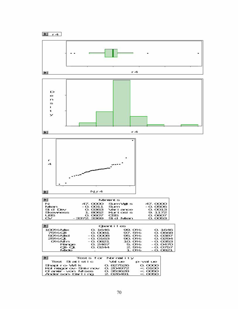
r4

r4

r4

Density

N_r4

r4




99. 0% 0. 1646 97. 5% 0. 0668 95. 0% 0. 0387 90. 0% 0. 0294 10. 0% -0. 0353 5. 0% -0. 0470 2. 5% -0. 0757 1. 0% -0. 0821



Val ue0. 8275260. 2049720. 3536282. 026491

p-val ue 0. 0000 <. 0100 <. 0050 <. 0050

70

r5

r5

r5

Density

N_r5

r5




99. 0% 0. 1376 97. 5% 0. 1064 95. 0% 0. 0920 90. 0% 0. 0811 10. 0% -0. 0562 5. 0% -0. 0789 2. 5% -0. 0806 1. 0% -0. 1290



Val ue0. 9877180. 0870380. 0475680. 283878

p-val ue 0. 8979 >. 1500 >. 2500 >. 2500

71

r6

r6

r6

Density

N_r6

r6




99. 0% 0. 1108 97. 5% 0. 0963 95. 0% 0. 0623 90. 0% 0. 0495 10. 0% -0. 0490 5. 0% -0. 0601 2. 5% -0. 0703 1. 0% -0. 0987



Val ue0. 9746210. 1101930. 0915110. 524577

p-val ue 0. 3925 >. 1500 0. 1443 0. 1802

72

r7

r7

r7

Density

N_r7

r7




99. 0% 0. 0343 97. 5% 0. 0214 95. 0% 0. 0158 90. 0% 0. 0139 10. 0% -0. 0110 5. 0% -0. 0136 2. 5% -0. 0137 1. 0% -0. 0167



Val ue0. 9642380. 0943730. 0749810. 495097

p-val ue 0. 1583 >. 1500 0. 2395 0. 2132

73

r8

r8

r8

Density

N_r8

r8




99. 0% 0. 0845 97. 5% 0. 0704 95. 0% 0. 0656 90. 0% 0. 0465 10. 0% -0. 0402 5. 0% -0. 0537 2. 5% -0. 0556 1. 0% -0. 0645



Val ue0. 9816650. 0842780. 0393250. 264965

p-val ue 0. 6620 >. 1500 >. 2500 >. 2500

74

r9

r9

r9

Density

N_r9

r9

Moment sN 47. 0000Mean -3. 129E-06St d Dev 0. 0280Skewness 0. 7097USS 0. 0361CV -894858. 91



99. 0% 0. 0882 97. 5% 0. 0507 95. 0% 0. 0469 90. 0% 0. 0417 10. 0% -0. 0291 5. 0% -0. 0396 2. 5% -0. 0459 1. 0% -0. 0585



Val ue0. 9640250. 1249900. 1013550. 579608

p-val ue 0. 1553 0. 0657 0. 1060 0. 1297

75

r10

r10

r10

Density

N_r10

r10




99. 0% 0. 1840 97. 5% 0. 1019 95. 0% 0. 0923 90. 0% 0. 0750 10. 0% -0. 0336 5. 0% -0. 0502 2. 5% -0. 0502 1. 0% -0. 0583



Val ue0. 9268530. 1151850. 1040730. 669338

p-val ue 0. 0058 0. 1184 0. 0973 0. 0795

76

Distribution of the difference of the VaR between the Delta-Normal method and the Historical Simulation method.

r1

r1

r1

Density

N_r1_1

r1




99. 0% 73. 2942 97. 5% 63. 3556 95. 0% 52. 2329 90. 0% 44. 3482 10. 0% -19. 6814 5. 0% -29. 1408 2. 5% -35. 3006 1. 0% -40. 8248



Val ue0. 9954990. 0502050. 1368410. 699356

p-val ue 0. 3050 0. 0155 0. 0375 0. 0712

77

Appendix D: SAS Results II Test for normality for the whole historical data of the portfolio of ten stocks from 01/02/2001 to 05/27/2003

r1

r1

r1

Density

N_r1

r1




99. 0% 0. 1538 97. 5% 0. 1272 95. 0% 0. 0806 90. 0% 0. 0545 10. 0% -0. 0411 5. 0% -0. 0573 2. 5% -0. 0705 1. 0% -0. 1058



Val ue0. 9356920. 0911481. 6756109. 804214

p-val ue 0. 0000 <. 0100 <. 0050 <. 0050

78

r2

r2

Density

N_r2

r2




99. 0% 0. 1092 97. 5% 0. 0866 95. 0% 0. 0671 90. 0% 0. 0495 10. 0% -0. 0433 5. 0% -0. 0592 2. 5% -0. 0846 1. 0% -0. 1207



Val ue0. 9537520. 0623550. 6953124. 475988

p-val ue 0. 0000 <. 0100 <. 0050 <. 0050

r2

79

r3

r3

r3

Density

N_r3

r3




99. 0% 0. 0607 97. 5% 0. 0421 95. 0% 0. 0346 90. 0% 0. 0238 10. 0% -0. 0225 5. 0% -0. 0326 2. 5% -0. 0458 1. 0% -0. 0610



Val ue0. 9203640. 1035662. 22515611. 76144

p-val ue 0. 0000 <. 0100 <. 0050 <. 0050

80

r4

r4

r4

Density

N_r4

r4



Quant i l es100% Max 0. 1646 75% Q3 0. 0132 50% Med 5. 848E-05 25% Q1 -0. 0139 0% Mi n -0. 1500 Range 0. 3146 Q3-Q1 0. 0271 Mode 0

99. 0% 0. 1250 97. 5% 0. 0714 95. 0% 0. 0547 90. 0% 0. 0348 10. 0% -0. 0346 5. 0% -0. 0482 2. 5% -0. 0671 1. 0% -0. 0915



Val ue0. 9193670. 1143772. 41179212. 95930

p-val ue 0. 0000 <. 0100 <. 0050 <. 0050

81

r5

r5

r5

Density

N_r5

r5




99. 0% 0. 3880 97. 5% 0. 2000 95. 0% 0. 1321 90. 0% 0. 0909 10. 0% -0. 0950 5. 0% -0. 1221 2. 5% -0. 1410 1. 0% -0. 1630



Val ue0. 8438750. 1008511. 88648711. 96463

p-val ue 0. 0000 <. 0100 <. 0050 <. 0050

82

r6

r6

r6

Density

N_r6

r6




99. 0% 0. 1290 97. 5% 0. 0963 95. 0% 0. 0763 90. 0% 0. 0590 10. 0% -0. 0532 5. 0% -0. 0678 2. 5% -0. 0801 1. 0% -0. 1065



Val ue0. 9760020. 0726860. 6525453. 475965

p-val ue 0. 0000 <. 0100 <. 0050 <. 0050

83

r7

r7

r7

Density

N_r7

r7




99. 0% 0. 0414 97. 5% 0. 0328 95. 0% 0. 0260 90. 0% 0. 0191 10. 0% -0. 0161 5. 0% -0. 0245 2. 5% -0. 0313 1. 0% -0. 0437



Val ue0. 9494850. 0654810. 8631405. 187065

p-val ue 0. 0000 <. 0100 <. 0050 <. 0050

84

r8

r8

r8

Density

N_r8

r8

Moment sN 599. 0000Mean 3. 257E-05St d Dev 0. 0373Skewness 0. 2204USS 0. 8302CV 114413. 276



99. 0% 0. 1100 97. 5% 0. 0840 95. 0% 0. 0684 90. 0% 0. 0456 10. 0% -0. 0429 5. 0% -0. 0548 2. 5% -0. 0684 1. 0% -0. 0900



Val ue0. 9745450. 0728230. 7045863. 902639

p-val ue 0. 0000 <. 0100 <. 0050 <. 0050

85

r9

r9

r9

Density

N_r9

r9




99. 0% 0. 1059 97. 5% 0. 0909 95. 0% 0. 0704 90. 0% 0. 0474 10. 0% -0. 0440 5. 0% -0. 0620 2. 5% -0. 0833 1. 0% -0. 1237



Val ue0. 9613120. 0813441. 2850697. 288738

p-val ue 0. 0000 <. 0100 <. 0050 <. 0050

86

r10

r10

r10

Density

N_r10

r10




99. 0% 0. 2374 97. 5% 0. 1554 95. 0% 0. 1023 90. 0% 0. 0676 10. 0% -0. 0669 5. 0% -0. 0910 2. 5% -0. 1154 1. 0% -0. 1417



Val ue0. 8695780. 1138232. 41462913. 79627

p-val ue 0. 0000 <. 0100 <. 0050 <. 0050

87

88

Documents

A study of the Delta Normal Method of Measuring VaR · PDF fileA study of the Delta Normal Method of Measuring VaR A Thesis Submitted to the Faculty ... Rajesh Kondapaneni _____ Date: