Embed Size (px)
Citation preview

Copyright is owned by the Author of the thesis. Permission is given for a copy to be downloaded by an individual for the purpose of research and private study only. The thesis may not be reproduced elsewhere without the permission of the Author.
A STUDY OF SOFTWARE
COMPONENT SYSTEM EVOLUTION
A thesis presented in partial fulfilment of the requirements for the
degree of
Doctor of Philosophy
in
Computer Science
at Massey University, Palmerston North,
New Zealand.
Graham Jenson
2013

ii
Abstract
There are an estimated 20 million users of the Ubuntu operating system and millions of
users of the Eclipse integrated development environment. Ubuntu and Eclipse systems
are constructed from components, called packages and bundles respectively, and can be
changed by adding or removing components to and from their systems. Over time
these systems will be continually changed to adapt to their software environment,
accommodate new user requirements, fix errors and/or prevent errors from occurring
in the future. This continual change is called the component system evolution process.
Using a developed simulation this thesis investigates the reduction of negative effects
during the component system evolution process. The primary negative effects that
are focused on are the amount of change made to the system, and the out-of-dateness
of the system. The simulation was created by modelling the evolution of component
systems and executed using a developed implementation. Various experiments that
simulate an Ubuntu system evolving over a year were conducted, and the change and
out-of-dateness of these systems measured. These experiments resulted in two novel
approaches that can be used to reduce change and out-of-dateness during evolution.
Therefore, this research could be used to reduce negative effects on millions of evolving
component systems.
iii

iv
Acknowledgements
I would like to thank my supervisors Jens Dietrich and Hans Guesgen. You have wisely
directed me throughout this project.
I would like to thank my office mates Jevon Wright and Fahim Abbasi. You have been
the continual distraction that allowed me to keep my sanity.
I would like to thank Stephen Marsland, Giovanni Moretti, Michele Wagner, Catherine
McCartin and Patrick Rynhart. You provided a community that made this task less
daunting.
I would like to thank my parents, Georgette and Deryk. You gave me my curiosity and
persistence.
Most importantly, I would like to thank Yuliya Bozhko. The completion of this thesis
is entirely due to your constant support and love.
v

vi
Contents
Abstract iii
Acknowledgements v
1 Introduction 1
1.1 Motivation . . . . . . . . . . . . . . . . . . . . . . . . . . . . . . . . . . 2
1.2 Objective . . . . . . . . . . . . . . . . . . . . . . . . . . . . . . . . . . . 3
1.3 Research Method . . . . . . . . . . . . . . . . . . . . . . . . . . . . . . . 3
1.3.1 Dataset . . . . . . . . . . . . . . . . . . . . . . . . . . . . . . . . 4
1.3.2 Methodology . . . . . . . . . . . . . . . . . . . . . . . . . . . . . 4
1.4 Contributions . . . . . . . . . . . . . . . . . . . . . . . . . . . . . . . . . 6
1.5 Thesis Overview . . . . . . . . . . . . . . . . . . . . . . . . . . . . . . . 7
2 Background 9
2.1 Software Evolution and Component-Based Software Engineering . . . . 10
2.1.1 Software Evolution . . . . . . . . . . . . . . . . . . . . . . . . . . 10
2.1.2 Component-Based Software Engineering . . . . . . . . . . . . . . 12
2.1.3 Unix and GNU/Linux Modular Operating Systems . . . . . . . . 14
2.2 Component Evolution vs. Component System Evolution . . . . . . . . . 15
2.2.1 Component Evolution . . . . . . . . . . . . . . . . . . . . . . . . 16
2.2.2 Component System Evolution . . . . . . . . . . . . . . . . . . . . 17
2.3 What is a Software Component? . . . . . . . . . . . . . . . . . . . . . . 18
2.3.1 The Definition of Software Component in this Thesis . . . . . . . 20
2.4 Component Models . . . . . . . . . . . . . . . . . . . . . . . . . . . . . . 21
2.4.1 OSGi . . . . . . . . . . . . . . . . . . . . . . . . . . . . . . . . . 21
2.4.1.1 Bundle Layer . . . . . . . . . . . . . . . . . . . . . . . . 22
2.4.1.2 Service Layer . . . . . . . . . . . . . . . . . . . . . . . . 22
2.4.1.3 OSGi Change . . . . . . . . . . . . . . . . . . . . . . . 23
2.4.1.4 OSGi Bundle Repostiory . . . . . . . . . . . . . . . . . 24
2.4.2 Eclipse Plugins . . . . . . . . . . . . . . . . . . . . . . . . . . . . 25
2.4.2.1 Eclipse Change . . . . . . . . . . . . . . . . . . . . . . . 26
vii
2.4.2.2 Eclipse P2 . . . . . . . . . . . . . . . . . . . . . . . . . 27
2.4.3 Fractal . . . . . . . . . . . . . . . . . . . . . . . . . . . . . . . . . 28
2.4.3.1 Fractal Change . . . . . . . . . . . . . . . . . . . . . . . 30
2.4.4 Maven . . . . . . . . . . . . . . . . . . . . . . . . . . . . . . . . . 31
2.4.4.1 Maven Change . . . . . . . . . . . . . . . . . . . . . . . 32
2.4.5 Debian Packages . . . . . . . . . . . . . . . . . . . . . . . . . . . 32
2.4.5.1 dpkg . . . . . . . . . . . . . . . . . . . . . . . . . . . . 33
2.4.5.2 apt-get . . . . . . . . . . . . . . . . . . . . . . . . . . . 33
2.4.6 SOFA 2.0 . . . . . . . . . . . . . . . . . . . . . . . . . . . . . . . 34
2.4.6.1 SOFA Change . . . . . . . . . . . . . . . . . . . . . . . 34
2.4.7 Common Upgradeability Description Format . . . . . . . . . . . 35
2.4.7.1 Mancoosi MPM . . . . . . . . . . . . . . . . . . . . . . 36
2.4.8 Comparison . . . . . . . . . . . . . . . . . . . . . . . . . . . . . . 37
2.5 Summary . . . . . . . . . . . . . . . . . . . . . . . . . . . . . . . . . . . 39
3 Formal Model of Component System Evolution 41
3.1 CoSyE Model of Component System Evolution . . . . . . . . . . . . . . 42
3.1.1 Evolution Problem . . . . . . . . . . . . . . . . . . . . . . . . . . 43
3.1.1.1 Complexity of an Evolution Problem . . . . . . . . . . 44
3.1.2 Constraints and Requests . . . . . . . . . . . . . . . . . . . . . . 45
3.1.3 Component System Evolution . . . . . . . . . . . . . . . . . . . . 47
3.1.4 Multiple Criteria Preferences . . . . . . . . . . . . . . . . . . . . 50
3.2 CUDF* Language . . . . . . . . . . . . . . . . . . . . . . . . . . . . . . 52
3.2.1 CUDF . . . . . . . . . . . . . . . . . . . . . . . . . . . . . . . . . 53
3.2.1.1 CUDF Language . . . . . . . . . . . . . . . . . . . . . . 53
3.2.1.2 Package Description . . . . . . . . . . . . . . . . . . . . 54
3.2.1.3 Preamble . . . . . . . . . . . . . . . . . . . . . . . . . . 55
3.2.1.4 Request . . . . . . . . . . . . . . . . . . . . . . . . . . . 56
3.2.2 CUDF Example . . . . . . . . . . . . . . . . . . . . . . . . . . . 57
3.2.3 Mancoosi Optimisation Format . . . . . . . . . . . . . . . . . . . 59
3.2.4 CUDF* . . . . . . . . . . . . . . . . . . . . . . . . . . . . . . . . 60
3.2.5 CUDF* Example . . . . . . . . . . . . . . . . . . . . . . . . . . . 61
3.3 Summary . . . . . . . . . . . . . . . . . . . . . . . . . . . . . . . . . . . 64
4 User Model 65
4.1 User Survey . . . . . . . . . . . . . . . . . . . . . . . . . . . . . . . . . . 66
4.1.1 Questions . . . . . . . . . . . . . . . . . . . . . . . . . . . . . . . 66
4.1.2 Results . . . . . . . . . . . . . . . . . . . . . . . . . . . . . . . . 67
4.1.3 Progressive vs. Conservative Users . . . . . . . . . . . . . . . . . 68
viii
4.2 SimUser model . . . . . . . . . . . . . . . . . . . . . . . . . . . . . . . . 69
4.2.1 Variables and Assumptions . . . . . . . . . . . . . . . . . . . . . 69
4.2.2 CUDF* Document Creation . . . . . . . . . . . . . . . . . . . . . 71
4.3 SimUser Data Collection and Conversion . . . . . . . . . . . . . . . . . . 72
4.3.1 Collecting the Components . . . . . . . . . . . . . . . . . . . . . 73
4.3.2 Probability a component will be selected . . . . . . . . . . . . . . 74
4.4 SimUser Validation . . . . . . . . . . . . . . . . . . . . . . . . . . . . . . 75
4.4.1 Randomness of SimUser . . . . . . . . . . . . . . . . . . . . . . . 75
4.4.2 Limitations of SimUser . . . . . . . . . . . . . . . . . . . . . . . 77
4.4.3 Perspective of the Ubuntu Repository . . . . . . . . . . . . . . . 78
4.5 Summary . . . . . . . . . . . . . . . . . . . . . . . . . . . . . . . . . . . 79
5 Resolving CoSyE Instances 81
5.1 Boolean Lexicographic Optimization Problem . . . . . . . . . . . . . . . 82
5.1.1 Boolean Satisfiability Problem (SAT) . . . . . . . . . . . . . . . 83
5.1.1.1 Pseudo-Boolean Extension of SAT to SAT+PB . . . . . 84
5.1.2 Boolean Lexicographic Optimization . . . . . . . . . . . . . . . . 86
5.1.3 Mapping CoSyE Instance to BLO Problems . . . . . . . . . . . . 87
5.1.4 Evolution Preference Order Mapping . . . . . . . . . . . . . . . . 89
5.2 Criteria . . . . . . . . . . . . . . . . . . . . . . . . . . . . . . . . . . . . 90
5.2.1 Change Criteria . . . . . . . . . . . . . . . . . . . . . . . . . . . 90
5.2.2 Out-of-date Criteria . . . . . . . . . . . . . . . . . . . . . . . . . 91
5.2.3 One Version per Package Criteria . . . . . . . . . . . . . . . . . . 93
5.3 Solving a BLO Problem . . . . . . . . . . . . . . . . . . . . . . . . . . . 93
5.3.1 Davis-Putnam-Logemann-Loveland Algorithm for SAT Solvers . 94
5.3.1.1 Unit Propagation . . . . . . . . . . . . . . . . . . . . . 95
5.3.1.2 Decide . . . . . . . . . . . . . . . . . . . . . . . . . . . 95
5.3.1.3 DPLL Advancements . . . . . . . . . . . . . . . . . . . 96
5.3.2 Iterative Strengthening . . . . . . . . . . . . . . . . . . . . . . . 96
5.3.3 Lexicographic Optimisation . . . . . . . . . . . . . . . . . . . . . 98
5.3.4 Resolving a CoSyE instance . . . . . . . . . . . . . . . . . . . . . 99
5.4 GJSolver . . . . . . . . . . . . . . . . . . . . . . . . . . . . . . . . . . . . 100
5.4.1 GJSolver Implementation . . . . . . . . . . . . . . . . . . . . . . 100
5.4.1.1 SAT4J . . . . . . . . . . . . . . . . . . . . . . . . . . . 101
5.4.2 Validation of GJSolver . . . . . . . . . . . . . . . . . . . . . . . . 102
5.4.2.1 Mancoosi International Solver Competition . . . . . . . 102
5.4.2.2 Tracks and Scoring . . . . . . . . . . . . . . . . . . . . 103
5.4.2.3 MISC Live . . . . . . . . . . . . . . . . . . . . . . . . . 104
5.4.2.4 MISC . . . . . . . . . . . . . . . . . . . . . . . . . . . . 104
ix
5.4.2.5 Analysis . . . . . . . . . . . . . . . . . . . . . . . . . . 105
5.5 Simulation Validation . . . . . . . . . . . . . . . . . . . . . . . . . . . . 105
5.5.1 Comparison to apt-get Logs . . . . . . . . . . . . . . . . . . . . 106
5.5.2 Comparison to Virtual System . . . . . . . . . . . . . . . . . . . 107
5.6 Summary . . . . . . . . . . . . . . . . . . . . . . . . . . . . . . . . . . . 108
6 Experiments, Results and Analysis 109
6.1 Users Choices to Upgrade and Install . . . . . . . . . . . . . . . . . . . . 110
6.1.1 Boundary Cases . . . . . . . . . . . . . . . . . . . . . . . . . . . 110
6.1.1.1 Results and Analysis . . . . . . . . . . . . . . . . . . . 111
6.1.2 Failures . . . . . . . . . . . . . . . . . . . . . . . . . . . . . . . . 113
6.1.2.1 Hard Failures . . . . . . . . . . . . . . . . . . . . . . . . 114
6.1.2.2 Soft Failures . . . . . . . . . . . . . . . . . . . . . . . . 114
6.1.3 Upgrade Probability Effects . . . . . . . . . . . . . . . . . . . . . 115
6.1.4 Install Probability Effects . . . . . . . . . . . . . . . . . . . . . . 118
6.2 Reduction of Out-of-dateness During Evolution . . . . . . . . . . . . . . 119
6.3 Reduction of Change During Evolution . . . . . . . . . . . . . . . . . . . 121
6.4 Realistic Evolution . . . . . . . . . . . . . . . . . . . . . . . . . . . . . . 123
6.4.1 Extracting Information from the User Submitted Logs . . . . . . 124
6.4.2 Simulation of Realistic Users . . . . . . . . . . . . . . . . . . . . 125
6.5 Answers . . . . . . . . . . . . . . . . . . . . . . . . . . . . . . . . . . . . 129
6.5.1 User Choices . . . . . . . . . . . . . . . . . . . . . . . . . . . . . 129
6.5.2 Reduce Out-of-dateness . . . . . . . . . . . . . . . . . . . . . . . 130
6.5.3 Reduce Change . . . . . . . . . . . . . . . . . . . . . . . . . . . . 130
6.5.4 Real Users . . . . . . . . . . . . . . . . . . . . . . . . . . . . . . 131
6.6 Summary . . . . . . . . . . . . . . . . . . . . . . . . . . . . . . . . . . . 131
7 Conclusion 133
7.1 Thesis Validation . . . . . . . . . . . . . . . . . . . . . . . . . . . . . . . 134
7.2 Future Research . . . . . . . . . . . . . . . . . . . . . . . . . . . . . . . 135
7.3 Closing Remark . . . . . . . . . . . . . . . . . . . . . . . . . . . . . . . . 136
A CUDF* Parsing to CoSyE Instance 137
A.1 CUDF* BNF Grammar . . . . . . . . . . . . . . . . . . . . . . . . . . . 137
A.2 Additional Stanza Constraints . . . . . . . . . . . . . . . . . . . . . . . . 139
A.3 Parsing . . . . . . . . . . . . . . . . . . . . . . . . . . . . . . . . . . . . 140
A.4 Components . . . . . . . . . . . . . . . . . . . . . . . . . . . . . . . . . . 140
A.5 Features . . . . . . . . . . . . . . . . . . . . . . . . . . . . . . . . . . . . 141
A.6 Package formula . . . . . . . . . . . . . . . . . . . . . . . . . . . . . . . 142
x

A.6.1 Sets of Package Formula . . . . . . . . . . . . . . . . . . . . . . . 143
A.7 System Constraints . . . . . . . . . . . . . . . . . . . . . . . . . . . . . . 143
A.7.1 Keep Constraints . . . . . . . . . . . . . . . . . . . . . . . . . . . 143
A.7.2 Dependency Constraint . . . . . . . . . . . . . . . . . . . . . . . 144
A.7.3 Conflict Constraint . . . . . . . . . . . . . . . . . . . . . . . . . . 145
A.8 Request . . . . . . . . . . . . . . . . . . . . . . . . . . . . . . . . . . . . 145
A.8.1 Install . . . . . . . . . . . . . . . . . . . . . . . . . . . . . . . . . 146
A.8.2 Remove . . . . . . . . . . . . . . . . . . . . . . . . . . . . . . . . 146
A.8.3 Upgrade . . . . . . . . . . . . . . . . . . . . . . . . . . . . . . . . 146
A.9 Criteria . . . . . . . . . . . . . . . . . . . . . . . . . . . . . . . . . . . . 148
B Full Criteria Mapping 149
B.1 -changed . . . . . . . . . . . . . . . . . . . . . . . . . . . . . . . . . . . . 150
B.2 -removed . . . . . . . . . . . . . . . . . . . . . . . . . . . . . . . . . . . 150
B.3 -new . . . . . . . . . . . . . . . . . . . . . . . . . . . . . . . . . . . . . . 151
B.4 -uptodatedistance . . . . . . . . . . . . . . . . . . . . . . . . . . . . . . . 151
B.5 -ovpp . . . . . . . . . . . . . . . . . . . . . . . . . . . . . . . . . . . . . 152
B.6 -unstable(d) . . . . . . . . . . . . . . . . . . . . . . . . . . . . . . . . . . 152
Bibliography 153
xi
List of Tables
2.1 Summary of presented component models’ constraints. . . . . . . . . . . 37
2.2 Summary of presented component models’ constraints description formats. 38
2.3 Summary of presented component models’ properties. . . . . . . . . . . 38
4.1 Summary of the survey respondents types and frequencies of interactions
with their package managers. . . . . . . . . . . . . . . . . . . . . . . . . 67
5.1 Example of the mapping from CoSyE criterion to a PB criterion. . . . . 90
5.2 Mapping of the change, removed and new criteria between MOF, CoSyE
and PB . . . . . . . . . . . . . . . . . . . . . . . . . . . . . . . . . . . . 91
5.3 Mapping of the up-to-date distance criterion between MOF, CoSyE and
PB . . . . . . . . . . . . . . . . . . . . . . . . . . . . . . . . . . . . . . . 93
5.4 Mapping of the one version per package criterion between MOF, CoSyE
and PB . . . . . . . . . . . . . . . . . . . . . . . . . . . . . . . . . . . . 93
5.5 Results from MISC 2011, (score (less is better) : time in seconds) . . . . 105
5.6 Comparison of installed packages between the collected apt-get logs and
the simulation. . . . . . . . . . . . . . . . . . . . . . . . . . . . . . . . . 107
5.7 Comparison of upgraded packages between the virtual Ubuntu 11.10
system and the simulation. . . . . . . . . . . . . . . . . . . . . . . . . . 107
6.1 Configuration of users that are the boundary cases in the simulation. . . 110
6.2 Configuration of users with variable probability to upgrade. . . . . . . . 115
6.3 Configuration of users with variable probability to install a component. 118
6.4 Configuration of progressive user that always upgrades. . . . . . . . . . 119
6.5 Mapping of the unstable criterion between MOF, CoSyE and PB . . . . 121
6.6 Configuration of users using the unstable criterion . . . . . . . . . . . . 122
6.7 Reduced change compared to the estimated reduced change of using the
unstable criterion. . . . . . . . . . . . . . . . . . . . . . . . . . . . . . . 123
6.8 Configuration of “realistic” users extracted from the submitted apt-get
logs . . . . . . . . . . . . . . . . . . . . . . . . . . . . . . . . . . . . . . 125
6.9 The mean final UTTDpC of the simulated“realistic”users using apt-get
and progressive criteria . . . . . . . . . . . . . . . . . . . . . . . . . . . . 127
xii
6.10 The mean total change of the simulated “realistic” users using apt-get
and progressive criteria . . . . . . . . . . . . . . . . . . . . . . . . . . . . 127
6.11 The mean estimated reduced change when using the unstable criterion
for the simulated “realistic” users using apt-get and progressive criteria 129
A.1 CUDF* Preamble properties . . . . . . . . . . . . . . . . . . . . . . . . . 139
A.2 CUDF* Package Description properties . . . . . . . . . . . . . . . . . . 139
A.3 CUDF* Request properties . . . . . . . . . . . . . . . . . . . . . . . . . 139
B.1 Mapping of the change, removed, new, one version per package, up-to-
date distance and unstable criteria between MOF, CoSyE and PB . . . 149
xiii
List of Figures
2.1 Example of OSGi Meta-data . . . . . . . . . . . . . . . . . . . . . . . . 22
2.2 Example of OSGi Declarative Services meta-data . . . . . . . . . . . . . 23
2.3 Example of OSGi Bundle Repository meta-data . . . . . . . . . . . . . . 24
2.4 Example of an Eclipse Plugin plugin.xml meta-data file . . . . . . . . . 26
2.5 Example of an Eclipse Plugin extension point schema file . . . . . . . . 27
2.6 Example of a simple Fractal ADL file . . . . . . . . . . . . . . . . . . . . 28
2.7 Example of a hierarchical Fractal ADL file . . . . . . . . . . . . . . . . . 29
2.8 Example of a Maven POM file . . . . . . . . . . . . . . . . . . . . . . . 31
2.9 Debian Control file for Text Editor . . . . . . . . . . . . . . . . . . . . . 32
2.10 Example of a Debian Control File for Spell Checker . . . . . . . . . . . 32
2.11 Example of a SOFA ADL Files . . . . . . . . . . . . . . . . . . . . . . . 35
2.12 Example of a CUDF file . . . . . . . . . . . . . . . . . . . . . . . . . . . 36
3.1 The relationships between CUDF* and CoSyE . . . . . . . . . . . . . . 42
3.2 Structure of the CUDF stanzas . . . . . . . . . . . . . . . . . . . . . . . 54
3.3 Structure of a CUDF stanza . . . . . . . . . . . . . . . . . . . . . . . . . 54
3.4 Example of Package Description Stanza . . . . . . . . . . . . . . . . . . 55
3.5 Example of preamble stanza demonstrating the extendable CUDF language 56
3.6 Example of CUDF request stanza . . . . . . . . . . . . . . . . . . . . . . 57
3.7 Example of a CUDF document . . . . . . . . . . . . . . . . . . . . . . . 58
3.8 Structure of the CUDF* stanzas . . . . . . . . . . . . . . . . . . . . . . 61
3.9 Example of a CUDF* document . . . . . . . . . . . . . . . . . . . . . . 62
4.1 Relationships between the SimUser model and CUDF* . . . . . . . . . . 65
4.2 The process to create a CUDF* document from a SimUser instance. . . 71
5.1 The relationships between the BLO problem and the CoSyE model . . . 82
5.2 The DPLL algorithm . . . . . . . . . . . . . . . . . . . . . . . . . . . . . 94
5.3 The Unit Propagation algorithm . . . . . . . . . . . . . . . . . . . . . . 95
5.4 The Iterative Strengthening algorithm . . . . . . . . . . . . . . . . . . . 97
5.5 The Lexicographic Iterative Strengthening algorithm . . . . . . . . . . . 98
5.6 The algorithm to resolve a CoSyE instance . . . . . . . . . . . . . . . . 100
xiv
5.7 The relationships within the GJSolver implementation . . . . . . . . . . 100
6.1 The UTTDpC of the simulated boundary case users. . . . . . . . . . . . 111
6.2 The total change of the simulated boundary case users. . . . . . . . . . 112
6.3 The UTTDpC of the variable upgrade users. . . . . . . . . . . . . . . . 116
6.4 The mean UTTDpC against of the frequency a user upgrades (1/u) . . 116
6.5 The mean total change of the variable upgrade users. . . . . . . . . . . . 117
6.6 The mean total change of the variable install users . . . . . . . . . . . . 119
6.7 The UTTDpC of the simulated progressive user. . . . . . . . . . . . . . 120
6.8 The UTTDpC of the simulated users using the unstable criterion . . . . 122
6.9 An extract of an apt-get log file . . . . . . . . . . . . . . . . . . . . . . 124
6.10 The upgrade and install probabilities of the submitted apt-get logs and
the “realistic” users . . . . . . . . . . . . . . . . . . . . . . . . . . . . . . 125
6.11 The UTTDpC for the simulated “realistic” users. Top: the apt-get
criteria users. Bottom: the progressive users. . . . . . . . . . . . . . . . 126
6.12 The mean total change for the simulated “realistic” users. Top: the
apt-get criteria users. Bottom: the progressive users. . . . . . . . . . . 128
A.1 CUDF* BNF Grammar . . . . . . . . . . . . . . . . . . . . . . . . . . . 138
xv
Chapter 1
Introduction
E pluribus unum – Latin for “Out of many, one”
de facto motto of the United States 1782 - 1956
The Greek philosopher Plutarch proposed in his work Life of Theseus a paradox that
is in essence the question1:
If an object has all its component parts replaced, is it the same object?
This question addresses many themes including how objects are made of components,
how they change their component parts, and what effect change has on the object in
question. Although ancient, these themes are still relevant today and this research
explores each of them in the domain of software.
How is a software system made from components? A component system can
be created by composing together software components (Szyperski, 2002). A
software component is an encapsulated unit that requires functionality supplied by
other components, in order to provide its own functionality. A component system is
valid only if every contained component has all its required functionality provided by
another component. For example, given that a text-editor component requires spell-
checker functionality, a valid system that includes the text-editor must also include a
component that provides spell-checker functionality.
How are component systems changed? A component system can be changed by
adding, removing or replacing components, however these actions must result in a
valid component system. This means that adding, removing, or replacing a single
1The actual question asked was whether Theseus’s ship, which was restored by replacing all woodenparts, remained the same ship.
1
CHAPTER 1. INTRODUCTION
component may cause a propagation of change to the component system. For example,
when adding a text-editor to a component system a component that provides spell-
checker functionality must also be added, otherwise the system will not be valid.
Additional complexity arises when changing a component system, as there may be more
than one way to change the system. Furthermore, different component systems may
have different properties and one system may be preferable to another. Therefore, when
changing a component system the resulting system should be valid and preferable. For
example, when a text-editor component is being added to a component system and
two components provide spell-checker functionality, a component system with either
spell-checker component is valid, however the component system selected should be
preferable to the other.
These complex and technical aspects of component system change can be automated.
Such automation allows users to change their component systems without performing
the tedious, error prone task of finding a preferable, valid component system. However,
when using such automated mechanisms a user must trust that the change will reflect
their preferences.
What effects does changing a component system have? Over time, a user will continually
change their system to meet their requirements and keep it up-to-date. This gradual
change is the component system evolution (CSE) process. The mechanisms by
which the systems are changed will effect the system as it evolves, particularly the
criteria by which preferable component systems are selected. However, what exactly
are the effects these mechanisms have on an evolving system is yet to be answered. This
research aims to provide answers to these questions by looking at component systems,
the mechanisms that change them, and CSE.
1.1 Motivation
Examples of popular component systems are the Ubuntu operating systems, which have
an estimated 20 million users2, and Eclipse integrated development environment (IDE),
which are used by thousands of companies and millions of users3. Ubuntu and Eclipse
systems are constructed from components, called packages and bundles respectively.
Ubuntu systems can be changed with the application apt-get (Barth et al., 2005) and
Eclipse systems can be changed with Eclipse P2 (Rapicault and Le Berre, 2010). These
allow the user to change their system by adding, removing and upgrading components.
2http://www.ubuntu.com/, accessed 16/5/20123http://www.eclipse.org/org/community survey/Eclipse Survey 2011 Report.pdf,
accessed 29/5/2012
2
CHAPTER 1. INTRODUCTION
Repeatedly applying such changes allows the Ubuntu and Eclipse systems to evolve
through the CSE process. By studying the CSE process and understanding the effects
it has on systems, this research has the potential to impact millions of users and their
systems.
1.2 Objective
The objective of this research is to study the process of component system evolution
and its effect on component systems. The primary effects that are focused on are the
amount of change made to systems and how out-of-date the systems become over time.
In section 4.1, these two effects are argued to be a users’ primary concerns during CSE.
Through understanding this change and out-of-dateness, this research aims to inform
developers and users of the consequences their choices have on evolving systems, and
reduce these negative effects.
The objective of this research has lead to the thesis:
It is possible to reduce the negative effects of component system evolution by
altering the mechanisms by which systems are changed.
The necessary steps to validate this thesis are:
• To develop a reproducible and controllable environment in which to measure the
effects of CSE.
• To use this environment to study how systems evolve.
• To alter the mechanisms by which systems are changed and study their impact
on CSE.
• To demonstrate a reduction on change and out-of-dateness using such alterations.
Once these steps are completed, this thesis will be shown to be supported.
1.3 Research Method
To study the evolution of a single component system, all changes to that system over a
period of time must be examined. Additionally, to gain a broad and useful perspective
of CSE characteristics, the evolution of many systems must be studied. To this end,
3
CHAPTER 1. INTRODUCTION
this research simulates the evolution of many Ubuntu systems. The reason for selecting
Ubuntu and simulation as the method of study are detailed further in this section.
1.3.1 Dataset
The Ubuntu operating system was selected as the component system to study CSE for
the following reasons:
• It has significant size and complexity which ensures that the results will not be
trivial.
• It has an active research community whose results can be used and built upon.
• It has an estimated 20 million users, potentially allowing the outcomes of this
research to have a significant impact.
• There are many open resources of information available to be collected and used
for simulation.
Another important question is “Why only Ubuntu?”, as only focusing on the evolution
of one component system may make the results from this research non-generalisable.
There are many similarities between component models (some are discussed in section
2.4) including the relationships between components and the mechanisms used to
change component systems. These similarities may make many of the contributions
from this research component system independent.
Another factor in the decision to only simulate the evolution of Ubuntu systems was the
lack of data available for other component models. Many systems, like Eclipse, do not
have their history archived as precisely as Ubuntu. This lack of available data meant
that data collection would be impractical or impossible. Therefore, the simulation of
other types of component system is not within the scope of this research, however the
simulation of further component systems is proposed as future research in section 7.2.
1.3.2 Methodology
The method selected to study CSE is to model its relevant aspects, then simulate the
evolution of many Ubuntu systems. This method was selected as a simulation provides
the necessary control over the variables of CSE to validate the thesis.
Another method that was considered when approaching this thesis was to study
the evolving systems of real users. The difficulty of this method would be finding
4
CHAPTER 1. INTRODUCTION
participants willing to allow experimental techniques to change their (possibly mission
critical) systems. Finding enough participants to produce meaningful results would
have required time and resources that were not available to this research. Additionally,
as evolution occurs over long periods of time, problems could take months to identify
and correct, increasing the risk when using this method for this research. Therefore,
the simulation approach to validating the thesis was preferred as it has a lower cost
and less risk.
The core hurdle in creating a simulation is ensuring that the returned results are similar
enough to reality to draw meaningful conclusions, i.e. the simulation is valid:
“Validation is the process of determining whether a simulation is an
accurate representation of the system, for the particular object of the study.”
(Law, 2005)
The methodology that Law (2005) outlines was selected because it gave practical
guidance to creating and using a valid simulation. The methodology was created
after the observation that validation was often “attempted after the simulation models
had already been developed” (Law, 2005). It was also observed that non-validated
simulations can produce erroneous information that leads to bad, possibly costly
decisions being made.
This methodology has a seven step approach to creating a valid simulation:
• Step 1: Formulate the problem: The problem should be described as clearly
as possible. The core artifacts at this stage are the overall objectives and the
scope of the study.
• Step 2: Collect information/data to construct a conceptual model: The
conceptual model is a description of how the simulation and system work in
relation to the study’s objectives. It contains all variables used to configure the
simulation.
• Step 3: Validate the conceptual model: The validation of the conceptual
model is accomplished through interviews and discussions with the stakeholders
of the study.
• Step 4: Implement the conceptual model: The implementation of the
conceptual model must be executed and documented in a way that allows others
to replicate and repeat the process.
5

CHAPTER 1. INTRODUCTION
• Step 5: Validate the simulation implementation: The most definitive way
to validate a simulation is to compare its results to those from an actual system
(Law, 2005).
• Step 6: Design, conduct and analyse experiments: Experiments use the
simulation to measure effects and test hypothesises. For each of the experiments,
the configuration and number of independent runs must be defined.
• Step 7: Document and present results: This presentation is required to
promote the future re-use of the models, through describing the validation process.
The above described methodology was created for large scale industrial projects with
substantial resources available. It describes the employment and use of experts and
analysts to ensure validity. The available resources for this project are fewer than these
large scale projects, therefore some of the steps have been decreased in scope. This may
reduce the validity of the final simulation, but these restrictions have been made only
when necessary, and done so in a manner that attempts to minimise negative effects.
1.4 Contributions
As stated above, CSE is studied through simulating the evolution of Ubuntu systems
guided by the methodology outlined by Law (2005). To accomplish this study, these
research questions must be answered:
• How can CSE be modeled?
• How can a user who changes their component system be modeled?
• How can a CSE simulation be implemented?
• How can the negative effects during CSE be reduced?
In answering these questions the contributions from this research are:
1. A formal model CoSyE (Component System Evolution) that describes CSE.
2. The CUDF* language that is used to define documents that describe the
evolution of a component system.
3. SimUser (Simulated User) that models a user who changes their system.
6
CHAPTER 1. INTRODUCTION
4. The GJSolver which is an efficient implementation that calculates the changes
made to a system as it evolves (called resolving). GJSolver was independently
validated through the MISC competition hosted by the Mancoosi project4.
5. A simulation of the evolution of Ubuntu operating systems using CoSyE,
CUDF*, SimUser and GJSolver.
6. Two methods to reduce the out-of-dateness and change during CSE.
7. The results, analysis and conclusions from experiments using the simulation.
These contributions overlap with published papers from this research:
1. An empirical study into the search space of resolving component systems (Jenson
et al., 2010a).
2. A formal framework to describe a users preferences during CSE (Jenson et al.,
2010b).
3. An empirical study into the evolution of component systems (Jenson et al., 2011).
1.5 Thesis Overview
This thesis is organised and presented in the order that resembles the steps of the above
described methodology: the problem is described (chapter 2), the models are presented
and validated (chapters 3 and 4), the implementation and validation of the simulation
are described (chapter 5), and the experiments and their results are discussed (chapter
6).
Chapter 2 explores the backgrounds of CSE and its related domains. This aims to put
CSE in historical context and to give suitable definitions to the elements of CSE.
Chapter 3 presents the CoSyE model and the CUDF* language that describe the formal
aspects of the evolution of component systems. CoSyE is used to describe the evolution
of a component system and CUDF* is used as the language to serialise CoSyE instances.
Chapter 4 presents the SimUser model which is used to describe users that request
changes to their component systems. This model includes assumptions and variables
that are necessary to simulate the evolution of Ubuntu systems. It is developed from
the results of a conducted survey. As this model relies on many assumptions that may
impact the validity of the simulation, the validation of this model is also discussed.
4http://www.mancoosi.org/, accessed 8/8/2012
7
CHAPTER 1. INTRODUCTION
Chapter 5 describes the algorithms used to create the GJSolver implementation. The
resolving of a component system can require significant computational effort, therefore
the algorithms and implementation used are an important aspect of research. The
verification of GJSolver and validation of the simulation are also discussed in this
chapter.
Chapter 6 describes the experiments, results and analysis that are conducted using
the developed simulation. The effects examined are the changes that the systems go
through, and how out-of-date the systems become during evolution. Through these
experiments, causes of additional change and out-of-dateness are identified. These
causes are addressed with some novel changes to CSE, and through using the simulation
the impact of these changes is measured. The effects of these changes are measured
using the simulation and are shown to have benefits during CSE.
This thesis concludes in chapter 7 by describing the contributions of this research and
possible future research.
8
Chapter 2
Background
In order to agree to talk, we just have to agree we are talking about roughly the
same thing.
The Feynman Lectures on Physics, Motion, Richard Feynman, 1961.
Software evolution (Lehman, 1980) is the process of repeated change made to a software
system to maintain it or to extend its functionality over the system’s lifetime. This
evolution process is necessary as any system must adapt to the changing software
environment, accommodate new user requirements, fix errors and/or prevent errors
from occurring in the future (ISO/IEC, 2006). Software maintenance and evolution
are often used interchangeably (Godfrey and German, 2008), however some differences
exist. One difference is that maintenance has connotations of a planned activity, where
evolution is the gradual refinement of a system (Lehman, 1980). That is, software
maintenance is a range of activities through which software is changed, and software
evolves as the system is repeatedly changed. This is similar to the definition given in
(Lehman, 1980).
A component system is created out of a set of components combined into a functioning
system by a composer (or assembler) (Szyperski, 2002). Apart from creating the
systems, composers are also responsible for changing their systems. This change can
be motivated by the same forces as software change, e.g. new system requirements. As
a composer makes changes to their component system over time, the system is said to
evolve.
This chapter illustrates the history and presents the state of the art of software
evolution, component systems, and CSE. Section 2.1 first describes the history and
connections between domains. Section 2.2 explores the separation of the evolution of
individual components and the evolution of component systems. The definitions of
9
CHAPTER 2. BACKGROUND
software components and component models used in this thesis are then presented in
section 2.3. To conclude this chapter, examples of various component models that fit
the given definitions are discussed in section 2.4.
2.1 Software Evolution and Component-Based Software
Engineering
The foundations for software evolution, software components, and component systems
were established in the late 1960s. The concept that would later become software
evolution was first described by Lehman (1969). The concept of software components
was proposed by McIlroy (1969). The operating system Unix (Raymond, 2003), whose
core philosophy is a modular system, was developed in 1969.
The domains of software engineering, software evolution and component-based software
engineering have gone through many advancements since their inceptions. This section
describes these advancements, building up to a discussion about CSE.
2.1.1 Software Evolution
Brooks (1975) states that over 90% of the cost of a system occurs after deployment in
the maintenance phase, and that any successful piece of software will inevitably need to
be maintained. This realisation, that software requires significant expense to maintain,
led researchers to study how software changed after its deployment. This is the study
of software evolution (Lehman, 1980).
In 1980, two fundamental empirical studies on the emerging domain of software
evolution were published. The first study by Lientz and Swanson (1980) explored the
activities that occur during software maintenance (later formalised in ISO/IEC 14764
(ISO/IEC, 2006));
1. Adaptive Maintenance: adapting to new system or technical requirements.
2. Perfective Maintenance: adapting to new user requirements.
3. Corrective Maintenance: fixing errors and bugs.
4. Preventive Maintenance1: adapting to prevent future problems.
1later added in taxonomies such as (IEEE, 1990)
10
CHAPTER 2. BACKGROUND
This study showed that around 75% of the maintenance effort was on the first two
types, and corrective maintenance took about 21% of the effort.
The second study by Lehman (1980) explored how evolution affected software. In this
study, Lehman described a set of laws that characterise software evolution:
1. Continuing Change: Software systems2 must be continually adapted, otherwise
they become progressively less satisfactory.
2. Increasing Complexity: As the system evolves its complexity increases unless work
is done to reduce it.
3. Self Regulation: The system evolves with statistically determinable trends and
invariances.
4. Conservation of Organisational Stability: The average effective activity rate to
evolve a system is invariant over its lifetime.
5. Conservation of Familiarity: As the system evolves, its incremental growth must
remain invariant to ensure users maintain mastery over the system.
6. Continuing Growth: The system must continually grow to maintain user
satisfaction.
7. Declining Quality: The quality of the system will decline unless rigorously
maintained.
8. Feedback System: The function a system performs is changed by the effect it has
on its environment.
Both the study from Lientz and Swanson (1980) and the laws from Lehman (1980)
argue that the software engineer’s objective of creating a satisfactory system is difficult,
expensive, and not always achievable. They state that the continual evolution of a
software system is necessary, and this evolution reduces quality, increases complexity,
and is costly.
From the perspective of software evolution, the software engineer’s goal is then to
create a system that can be quickly altered to adapt to a changing environment while
working to reduce the inevitable complexity caused by changing software. Towards
such goals, iterative development processes have been created, such as the spiral
development method (Boehm, 1988). This process describes the stages of development
2Lehman calls them E-type systems: software implemented in a real-world computing context(Lehman, 1980)
11
CHAPTER 2. BACKGROUND
as communication, planning, modeling, construction, and deployment. These stages
are continually iterated until the software project is no longer actively maintained.
The practical problems of software evolution can be seen in the struggle with legacy
software (Bennett, 1995). Legacy software is functional software that is old and
outdated, but it has not been replaced due to its critical status, not being well
understood, or the cost of redesigning. A piece of software is described as “legacy”
if it cannot be maintained (due to its complexity or size) within an acceptable cost
(Bisbal et al., 1999). As a legacy system does not evolve, new user and technical
requirements cannot be fulfilled, and the satisfaction with the system will decrease over
time. This has led the problem of legacy software to be described as enduring (Bennett
and Rajlich, 2000).
Software evolution is still seen as a young field (Godfrey and German, 2008), as many
open questions remain unanswered. Recent empirical studies that explore the cost of
software evolution are summarised by Grubb and Takang (2003), showing that the costs
of software maintenance range from 49% to 75%, and that these costs have not fallen
since the 1970’s. To lower the cost of software evolution, various methods and tools
have been proposed. For example, agile software development methodologies (The Agile
Alliance, 2001) are defined to encourage rapid and flexible responses to change, and
refactoring tools (Fowler and Beck, 1999; Murphy-Hill and Black, 2008) have been
developed to restructure code to decrease complexity and increase maintainability.
Another way of lowering costs of the software evolution process is to create systems
from encapsulated units called software components (Szyperski, 2002).
Current explorations of the history, and state-of-the-art, of software evolution are
presented by Bennett and Rajlich (2000), Lehman and Ramil (2003), and Godfrey and
German (2008). In all these papers, the importance of software evolution is emphasised,
and the need for more knowledge about the evolution process and its properties is
discussed.
2.1.2 Component-Based Software Engineering
The concept of Component-Based Software Engineering (CBSE) was first outlined by
McIlroy (1969), by describing the idea of a software components subindustry which
created components to be used in software. This report is an expansion on an earlier
idea for pipes (McIlroy, 1964), where McIlroy described designing software to fit
together, like screwing a hose to a tap.
The reuse of code to decrease development time was originally the major perceived
benefit of using software components. Later, other benefits of constructing systems
12
CHAPTER 2. BACKGROUND
from modular components were identified by Parnas (1972):
• Managerial Separation: the ability to develop components in separate groups
with little communication.
• Product Flexibility : the ability to make drastic changes to one component, without
changing others.
• Comprehensibility : the ability to study the system one module at a time.
The “software component” concept was soon picked up by other researchers such as
Yourdon and Constantine (1976), who described their ideas on structured design as:
• The art of designing the components of a system and the interrelationship between
those components in the best possible way.
• The process of deciding which components are interconnected in which way to
solve some well-specified problem.
Yourdon and Constantine (1976) list the goals of structured design as efficiency,
maintainability, modifiability, generality, flexibility, and utility. These goals are aimed
to be achieved by dividing the system into functional units that can be treated
independently. Each unit corresponds to exactly one small well-defined piece of the
system, and the units relationship corresponds to a relationship between pieces of the
system.
A problem soon emerged as the number of software components grew, where the best
set of components that satisfy the requirements of the system must be selected. Prieto-
Diaz and Freeman (1987) described this as the selection problem, where a composer
can have many alternative compositions of components to select from. This increases
the effort required to use software components as each possible combination must be
examined and ranked based on how well they match the composer’s specifications.
Current research into solutions to the selection problem asks the questions of:
• How to describe a component and its attributes (Treinen and Zacchiroli, 2009a;
Xinjuan et al., 2007)?
• How to search for compositions that fit a set of requirements (Abate and DiCosmo,
2011; Kwong et al., 2010; Treinen and Zacchiroli, 2009b; de Almeida et al., 2004)?
• How to rank a particular composition (Chen et al., 2011; Aleti et al., 2009)?
13
CHAPTER 2. BACKGROUND
The current state of CBSE is fractured, where there are many different component
frameworks (some presented in section 2.4), each with different goals and attributes.
Additionally, the original concept of a software component subindustry has never truly
come to fruition (Szyperski, 2002). A possibility for this is the unsure definitions of what
software components are (Crnkovic et al., 2011). The hope for CBSE, as described by
Crnkovic et al. (2011), is that the technology and research will converge, and terms and
concepts in the software component domain will become standardised. This problem
is later described in section 2.3, where the software component definition in this thesis
will be discussed.
2.1.3 Unix and GNU/Linux Modular Operating Systems
The research into software components by McIlroy (1969) coincided with his help in the
development of the operating system Unix (Raymond, 2003). McIlroy had significant
impact not only on the implementation of Unix, where many of his ideas like pipes
where included, but also on the Unix philosophy. McIlroy’s Unix philosophy has been
summarised as:
“Write programs that do one thing and do it well. Write programs to work
together. Write programs to handle text streams, because that is a universal
interface.” (Salus, 1994)
This philosophy led to the first two rules (out of fifteen) of Unix (Raymond, 2003):
• Rule of Modularity : Write simple parts connected by clean interfaces.
• Rule of Composition: Design programs to be connected to other programs.
To eliminate the perceived problems of the proprietary Unix system, in 1983 Richard
Stallman created the GNU project (Stallman and Others, 1985) to implement a free
Unix-like operating system. With a kernel developed by Linus Torvalds based on
the MINIX operating system (Tanenbaum, 1989), the GNU/Linux operating system
(Torvalds and Diamond, 2002) was created. GNU/Linux is seen as a return to the
original philosophy of Unix (Gancarz, 2003), where the creation of small modular
programs that interact is central. Aligned with this philosophy, a distribution of
GNU/Linux called Debian (Barth et al., 2005) was announced in 1993. This release
came with the Debian Manifesto (Murdock, 1994) that stated that Debian would be
constructed from high quality components (or packages) which can be maintained by
experts.
14
CHAPTER 2. BACKGROUND
Initially, a significant amount of technical expertise was required to change the
composition of packages in a Debian system. Each package had a set of constraints
that described the systems that it would be functional in and whenever a change was
made, these constraints where required to be satisfied. Not only was satisfying these
constraints difficult, but selecting an appropriate system was also a problem (due to
the selection problem discussed earlier in section 2.1.2). For example, installing a new
package required satisfying all its constraints, and if there were multiple systems that
satisfied these constraints, one would have to be chosen.
With the release of the application apt-get in the late 1990’s, the necessary technical
knowledge to compose or change a Debian system was significantly reduced. A user
could request apt-get to change their system, and it would find, select then change to a
new composition that satisfies the request and component constraints. This automated
the search for a satisfactory solution, solving the problem which had restricted the
evolution of Debian systems prior to apt-get’s release. The apt-get package manager
and similar applications have been called the “single biggest advancement Linux has
brought to the industry” (Murdock, 2007) because it has made it “far easier to push
new innovations out into the marketplace and generally evolve the OS”. Such lowering
of the technical knowledge required to become a composer of a component system has
had other effects that are discussed in the next section.
2.2 Component Evolution vs. Component System Evolu-
tion
Originally it was assumed that developers were the composers (Parnas, 1972; Prieto-
Diaz and Freeman, 1987) of component systems. That is, developers would compose,
verify, then release a component system to users. However, with applications like
apt-get the user has started to play the role of the composer for their systems. A
user, without technical knowledge, can now change the composition of their component
system to satisfy their requirements.
The situation where the user is the composer of the system has been called system
tailoring (Mørch, 1997) and end-user assembly (Szyperski, 2002). It has been noted
that the potential of component systems have increased with this user composition
(Szyperski, 2002) as the user can craft solutions without requiring expert assistance.
However, a system is also more fragile as the quality of a system may not be verifiable
by a non-technical user.
When the user is the composer of their system, it breaks apart two important processes,
15
CHAPTER 2. BACKGROUND
component evolution and CSE. The developer, rather than the composer of the
component system, is now solely in charge of evolution of the components they maintain.
In this section, the differences between, and the impact of separating, component
evolution and CSE are discussed.
2.2.1 Component Evolution
Component evolution is the process by which components change over time through
continual maintenance. This maintenance requires technical knowledge of the internal
workings and structure of the component, therefore it must be accomplished by a
developer. This makes component evolution similar to software evolution as it is a
process driven by developers. A significant difference between software evolution and
component evolution occurs because a developer has limited control over the system in
which their component is used. This difference makes validating a component difficult
as testing all possible systems it can be deployed in may be practically impossible.
To allow the developer to describe valid compositions their component will be functional
in, they are typically provided a means of expressing constraints. These constraints can
describe conflicts between components, and/or dependencies on other components. For
example, if a component a requires component b to be included in the composition for
a to be functional, a is said to depend on b. Further, if a requires that component c
not be in the composition, it is said that a conflicts with c. Such constraints are used
to ensure that a component system that includes a is valid.
The developer may not have control over the evolution of components it depends on or
conflicts with. Therefore, any constraint a component has on another may only be valid
for a particular state, or range of states, of the other components. Such component
states are tagged with versions, these provide an order to the evolution of a component.
For example, a component a which is version 1, is less evolved than the component a
version 2. Further consider, a version 1 depends on b version 1, and a version 2 depends
on b version 2.
This discussion on component evolution describes some differences to software
evolution. It is given not as a complete exploration of this domain but an introduction.
A proper methodology for the development and evolution of software components is
still being sought (Szyperski, 2002). Discussions on types of evolutionary changes with
comparisons to other domains are given in (Papazoglou et al., 2011), and empirically
explored by Vasa et al. (2007).
16
CHAPTER 2. BACKGROUND
2.2.2 Component System Evolution
A component system is changed when its composer alters the system’s composition
of components. The system evolves over time as these changes are repeatedly made.
As described in ISO/IEC 14764 (ISO/IEC, 2006), these changes could be adaptive,
perfective, corrective or preventive. However, unlike the changes in software evolution
or component evolution, CSE can only make changes by adding or removing components
that already exist. For example, a composer could not change the system to satisfy a
requirement if no component has yet been developed to satisfy that requirement.
Changing a component system is restricted by the constraints that components use to
describe valid compositions. It would be very difficult for a non-technical user to alter
a composition without some tool support. In this research such functionality is called
Component Dependency Resolution (CDR). CDR helps the composer alter their
system by satisfying their requests for change with valid compositions. Additionally,
the returned compositions satisfy some preferences. For example, suppose a user wants
to install a new text-editor component into their system, and the selected text editor
has a dependency on a spell-checker. A preference to be up-to-date means that the
most recent version of components should be selected. A system that provides CDR
functionality would try to find a valid system that has up-to-date versions of a text-
editor and a spell-checker.
CDR functionality is currently available for Eclipse provided by the P2 provisioning
system (Rapicault and Le Berre, 2010) and the package manager apt-get for the
Debian GNU/Linux distribution (Barth et al., 2005). CDR functionality can be used
at design time to determine the required dependencies to build and test a project (as
in Apache Maven (Porter et al., 2008)), at run time to evolve or extend a component-
based system (as in Eclipse P2 (Rapicault and Le Berre, 2010)), or it can be used to
build and restructure software product lines (Savolainen et al., 2007).
CDR systems typically provide similar functionality that allow the user to install
and remove components, adding or removing a component to or from the system.
Furthermore, typically provided is an upgrade function that removes then installs a
higher version of the same component. For example, to upgrade the components in a
Debian GNU/Linux system, the command apt-get upgrade is all that is needed to
be executed. To extend the system to install a component comp the command apt-get
install comp can be executed. The simplicity that CDR provides enables users to
become composers of their component systems.
A problem arises during component system evolution when trying to measure the
evolved state of a component system. A component system is a set of components,
17
CHAPTER 2. BACKGROUND
where each component can have different versions. This may make a component system
impossible to version in a way similar to how individual components are versioned. For
example, a system that has version 1 of component a and version 2 of component b, is
neither more or less out-of-date than a system with version 2 of a and version 1 of b.
This can get even more complicated when considering some component models allow
multiple versions of a single component installed, e.g. is a system with version 1 and 2
of a installed less evolved that a system with only version 2 of a installed?
Component system evolution is empirically studied by Fortuna et al. (2011) who look at
the first ten releases of Debian and compare it to the evolution within biology. Methods
to change component systems are discussed in (Ryan and Newmarch, 2005) and (Luo
et al., 2004), and the mitigation of the negative effects caused by such evolution is
discussed in the paper (Stuckenholz, 2007). This thesis contributes a formal model of
component system evolution in chapter 3.
2.3 What is a Software Component?
How a “software component” is defined will impact how CSE is studied and discussed.
It is difficult to find a precise definition of a software component as the intuitive concept
may be quite different from any model or implementation (Crnkovic et al., 2011).
Finding a definition that satisfies all parties may be an impossible task. However, by
defining a software component with respect to component system evolution, this process
can be studied without the paralysis of finding a complete definition. In this thesis,
a software component is defined to have explicitly declared constraints and include
mechanisms to automatically alter a component composition. These two attributes are
seen as sufficient to allow CDR to be used, and allow a user to be the composer and
change their system.
A component describes a part or element of a larger system or process. A broad
characterisation of a component is “components can be composed together”. They
can be physical, as in electrical or mechanical components, or virtual, as in software
components. Typically, components can be used in many different contexts. For
example, a resistor component, they can be used in electrical systems from space
stations to cellphones. This concept of what a component is has led to problems in
defining the concept of a software component.
A discussion between two researchers in component software, Bertrand Meyer and
Clemens Szyperski, highlighted the difficultly of defining “software component”. They
converse across the articles Meyer (1999); Szyperski (2000b,a); Meyer (2000), discussing
18

CHAPTER 2. BACKGROUND
their definitions of what a software component is.
Szyperski defines a component (Szyperski, 2002) as having three characteristic
properties:
1. Being a unit of independent deployment.
2. Being a unit of third party composition.
3. Having no externally observable state.
Meyer’s definition of software components is enumerated as one that:
1. May be used by other software elements (clients).
2. May be used by clients without the intervention of the components’ developers.
3. Includes a specification of all dependencies (hardware and software platform,
versions, other components).
4. Includes a precise specification of the functionality it offers.
5. Is usable solely on the basis of that specification.
6. Is composable with other components.
7. Can be integrated into a system quickly and smoothly.
Others, like (Heineman and Councill, 2001), have stated that components must conform
to a component model:
“A software component is a software element that conforms to a
component model and can be independently deployed and composed
without modification according to a composition standard.”
Furthermore, they define a component model as:
“A component model defines a set of standards for component
implementation, naming, interoperability, customization, composition,
evolution, and deployment.”
Exactly what is, and what is not a software component is in dispute amongst the
community, and a definitive description of a software component is elusive (Vasa et al.,
19
CHAPTER 2. BACKGROUND
2007). As such, many different component models have been developed, each targeting
various domains with different functionality and technical aspects. This diversity
has inspired a classification approach (Crnkovic et al., 2011), where components and
component models are classified into a scheme. This effort highlights the difficulty in
creating an exact definition of a software component.
The problems encountered when trying to precisely define a software component may
stem from the fact that “component” is a broad concept. The problem, as observed
from the area of formal concept analysis (Ganter and Wille, 1999) by (Szyperski, 2002),
is that it is impossible to “enumerate a fixed agreeable set of features that is necessary
and sufficient for a natural concept such as component.”
However, a definition can be found, not by feature enumeration but through stating
the intention for the concept and exploring the technically inevitable consequences
(Szyperski, 2002). As the intention of this thesis is to investigate component system
evolution, the definition of software component will be with respect to this process.
2.3.1 The Definition of Software Component in this Thesis
The definition of a software component is given with respect to the evolution of a
component system using component dependency resolution. Both these areas have
already been discussed in this chapter and will be used to define the concept of“software
component”. This definition specifies the type of components and component models
this research can be applied to.
In this thesis a software component is defined as a unit of independent deployment,
and third party composition, and a component model must:
1. Require the explicit definition of component constraints that describe composi-
tions that are valid.
2. Include mechanisms in which to programmatically change a component system.
To allow CDR functionality to alter a component system, the component constraints
must be explicitly defined and computer readable, and an interface must be provided by
the component system to be changed. This definition will allow the study of component
system evolution as a user changes their system using CDR functionality.
This definition leaves many aspects of a software components undefined, as can be seen
when compared to the classification from (Crnkovic et al., 2011). Most aspects of a
component model are ignored as they are superfluous to the core topic of this research.
20
CHAPTER 2. BACKGROUND
This makes the definition in this research broadly applicable, while also being focused
on CSE.
The next section explores this definition of software component by discussing different
component models that conform to it.
2.4 Component Models
Given the definition of a software component in this thesis, some current component
models are described and discussed. These models come from industry (OSGi, Eclipse
Plugins, Fractal, Maven), the open source community (Debian) and academia (SOFA2,
CUDF).
For these component models to conform to the previously described definition their
components must explicitly describe their constraints and they must provide a
mechanism to alter the systems composition. The typical method in which components
from these models express their constraints is through meta-data files, and to alter
compositions some low level interface is provided. These meta-data files and interfaces
are described and discussed, as is any CDR functionality that may be provided.
To compare these component models, the example of a text editor component that
depends on a spell checker component is used. It is hoped this simple situation will
highlight the similarities and differences between the various component models.
2.4.1 OSGi
OSGi is a mature component model from the OSGi Alliance. It has implementations
from organizations like the Eclipse Foundation with their Equinox framework (McAffer
et al., 2010), and the Apache foundation with their framework Felix3.
OSGi components are referred to as bundles, each contains a meta-data file describing
the bundle’s constraints, and a set of Java packages and classes as implementation. The
OSGi framework separates the components for deployment and run-time into bundles
and services respectively. These services exist on a separate layer to the bundles, each
service is created at run-time and is represented by a Java object. This service layer can
also describe constraints through frameworks like Spring Dynamic Modules4. Under
the definition of component in this research, this makes both the bundle layer and the
service layer software component models. These layers are discussed here.
3http://felix.apache.org/ accessed 6/3/20124http://www.springsource.org/osgi accessed 6/3/2012
21
CHAPTER 2. BACKGROUND
2.4.1.1 Bundle Layer
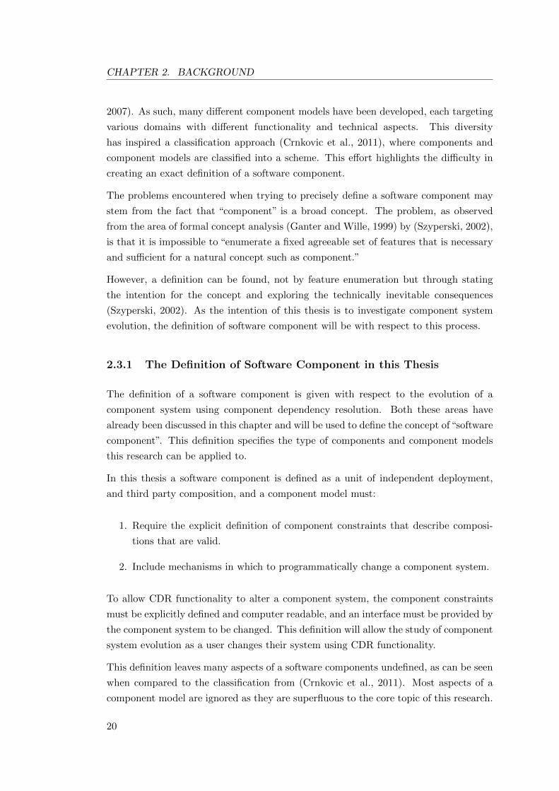
To show how the bundle meta-data describe constraints of a component, an example is
presented in figure 2.1 where a text editor bundle depends on a spell checker.
Bundle-Name: TextEditor
Bundle-Vendor: Graham Jenson
Bundle-SymbolicName: nz.geek.textEditor
Bundle-Version: 0.0.1.alpha
Bundle-RequiredExecutionEnvironment: J2SE-1.4
Export-Package: nz.geek.textEditor;version="0.0.1.alpha"
Require-Bundle: nz.geek.fonts
Import-Package: nz.geek.spellchecker;version>"0.0.1"
Figure 2.1: Example of OSGi Meta-data
This meta-data shows the name and version of the component, as well as the exported
packages (referring to Java packages). Also presented are constraints, such as the
necessary execution environment, and the required bundles and packages in the system.
Require-Bundle describes the direct dependence on other bundles, and Import-
Package describes the dependence on packages provided by other bundles.
2.4.1.2 Service Layer
This bundle meta-data only contains information necessary for the execution of a
component. However, for the component to be functional the service layer of OSGi
is used.
The service layer is defined in the core OSGi specification (The OSGi Alliance, 2007b),
however its definition does not describe any meta-data format. To help manage services,
a number of frameworks have emerged, e.g. Spring Dynamic Modules5. OSGi’s
compendium specification (The OSGi Alliance, 2007a) also defines a service layer meta-
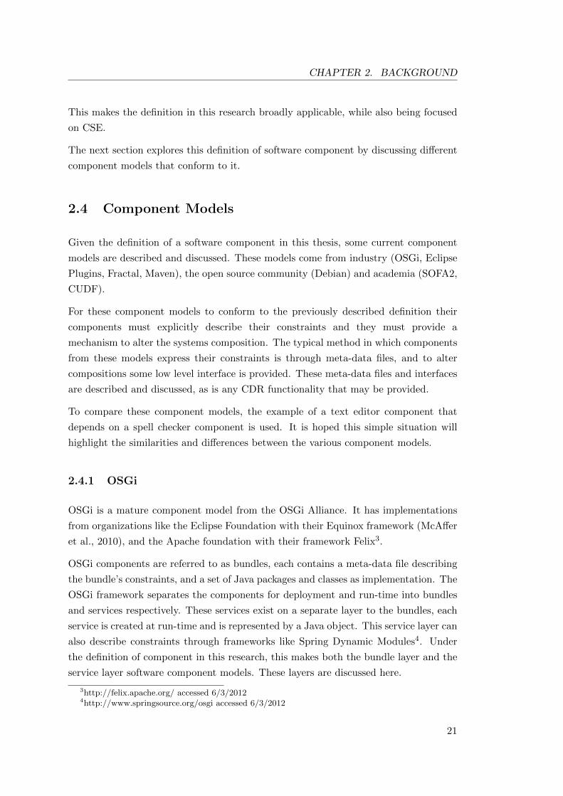
data format called Declarative Services (DS). To show how the DS meta-data can be
used to express constraints on the service layer, an example is presented in figure 2.2.
This meta-data includes references to implementation elements (like interfaces) that
are provided and required, and methods to interact with the services. The dependency
constraints can have cardinalities, e.g. a text editor can use multiple spell checkers.
5http://www.springsource.org/osgi accessed 6/3/2012
22
CHAPTER 2. BACKGROUND
<?xml version="1.0"?>
<component name="textEditor">
<implementation class="nz.geek.textEditor.TextEditorImpl"/>
<service>
<provide interface="nz.geek.textEditor.TextEditor"/>
</service>
<reference name="spellChecker"
interface="nz.geek.spellchecker.SpellChecker"
bind="setSpellChecker"
unbind="unsetSpellChecker"
cardinality="0..1"
policy="dynamic"/>
</component>
Figure 2.2: Example of OSGi Declarative Services meta-data
The service tag describes the services provided, and the reference tag expresses a
dependence on another service.
One aspect lacking in the DS meta-data is the ability to define a version range on
constraints. The version of a service is implicitly defined by the version of the bundle
that provides the service. However, this implicit version is unable to be reasoned about
by DS.
2.4.1.3 OSGi Change
The programmatic evolution of an OSGi system is defined in the interfaces created by
the OSGi alliance.6 The installation and removal of both the bundles and services from
the OSGi system are:
• To install a bundle:
org.osgi.framework.BundleContext#install
• To uninstall a bundle:
org.osgi.framework.Bundle#uninstall
• To register a service:
org.osgi.framework.BundleContext#registerService
6http://www.osgi.org/javadoc/r4v43/ accessed 6/3/2012
23
CHAPTER 2. BACKGROUND
• To unregister a service:
org.osgi.framework.ServiceRegistration#unregister
These methods can be used from an implemented console, allowing a user to directly
execute them to add or remove bundles.
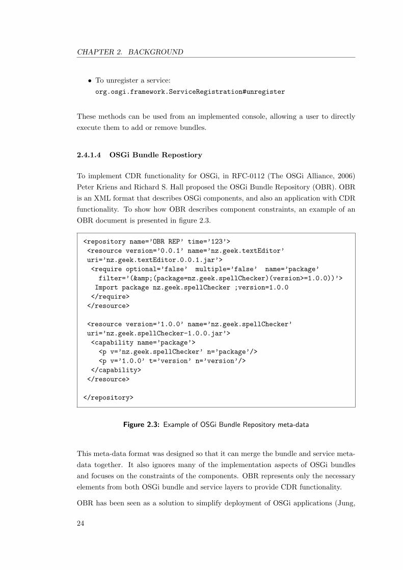
2.4.1.4 OSGi Bundle Repostiory
To implement CDR functionality for OSGi, in RFC-0112 (The OSGi Alliance, 2006)
Peter Kriens and Richard S. Hall proposed the OSGi Bundle Repository (OBR). OBR
is an XML format that describes OSGi components, and also an application with CDR
functionality. To show how OBR describes component constraints, an example of an
OBR document is presented in figure 2.3.
<repository name=’OBR REP’ time=’123’>
<resource version=’0.0.1’ name=’nz.geek.textEditor’
uri=’nz.geek.textEditor.0.0.1.jar’>
<require optional=’false’ multiple=’false’ name=’package’
filter=’(&(package=nz.geek.spellChecker)(version>=1.0.0))’>
Import package nz.geek.spellChecker ;version=1.0.0
</require>
</resource>
<resource version=’1.0.0’ name=’nz.geek.spellChecker’
uri=’nz.geek.spellChecker-1.0.0.jar’>
<capability name=’package’>
<p v=’nz.geek.spellChecker’ n=’package’/>
<p v=’1.0.0’ t=’version’ n=’version’/>
</capability>
</resource>
</repository>
Figure 2.3: Example of OSGi Bundle Repository meta-data
This meta-data format was designed so that it can merge the bundle and service meta-
data together. It also ignores many of the implementation aspects of OSGi bundles
and focuses on the constraints of the components. OBR represents only the necessary
elements from both OSGi bundle and service layers to provide CDR functionality.
OBR has been seen as a solution to simplify deployment of OSGi applications (Jung,
24
CHAPTER 2. BACKGROUND
2007), distribution and deployment to embedded ubiquitous systems (Jung and Chen,
2006), smart home applications (Gouin-Vallerand and Giroux, 2007) and dynamic
distribution of drivers (Kriens, 2008).
The most mature implementation of an OBR client is offered by the Apache foundation.
The client is bundled with their core OSGi framework Apache Felix. This client can be
used with any of the large public or private OBR collections of bundles. An example of
one such public repository is the Paremus repository7 which contains (as of December
2011) over 2000 bundles.
The specification of OBR does not define a method or parameters used to define
preferences when selecting a component system. Therefore, selecting systems, when
many are valid, is implementation specific. The method used by the Apache OBR8
implementation to select a system is described on its help page as:
“OBR might have to install new bundles during an update to satisfy
either new dependencies or updated dependencies that can no longer be
satisfied by existing local bundles. In response to this type of scenario,
the OBR deployment algorithm tries to favor updating existing bundles, if
possible, as opposed to installing new bundles to satisfy dependencies.”
This shows that when upgrading a system, not installing new bundles is preferred.
2.4.2 Eclipse Plugins
Eclipse is a widely used integrated development environment (IDE) and an extensible
plugin platform for creating Java applications. It is built on top of the OSGi framework,
but re-implements OSGi’s service layer with its own Eclipse plugin runtime. Therefore,
the distributed components are OSGi bundles and the run time elements are plugin
services.
These plugins are defined using extensions and extension points, where extensions
provide a service for an extension point. To show how plugin meta data is used to
define constraints, an example is presented in figure 2.4.
This plugin defines the name and version of the plugin, and using the tag requires
defines the requirements of this plugin to function. The extension-point tag defines
not only what the plugin provides, but also the required information in order to provide
it, described in a schema. This is a special feature of the Eclipse plugin framework,
7http://www.osgi.org/Repository/ accessed 6/3/20128http://felix.apache.org/site/apache-felix-osgi-bundle-repository.html accessed 6/12/2011
25
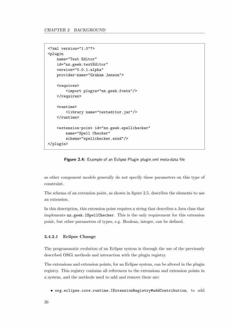
CHAPTER 2. BACKGROUND
<?xml version="1.0"?>
<plugin
name="Text Editor"
id="nz.geek.textEditor"
version="0.0.1.alpha"
provider-name="Graham Jenson">
<requires>
<import plugin="nz.geek.fonts"/>
</requires>
<runtime>
<library name="texteditor.jar"/>
</runtime>
<extension-point id="nz.geek.spellchecker"
name="Spell Checker"
schema="spellchecker.exsd"/>
</plugin>
Figure 2.4: Example of an Eclipse Plugin plugin.xml meta-data file
as other component models generally do not specify these parameters on this type of
constraint.
The schema of an extension point, as shown in figure 2.5, describes the elements to use
an extension.
In this description, this extension point requires a string that describes a Java class that
implements nz.geek.ISpellChecker. This is the only requirement for this extension
point, but other parameters of types, e.g. Boolean, integer, can be defined.
2.4.2.1 Eclipse Change
The programmatic evolution of an Eclipse system is through the use of the previously
described OSGi methods and interaction with the plugin registry.
The extensions and extension points, for an Eclipse system, can be altered in the plugin
registry. This registry contains all references to the extensions and extension points in
a system, and the methods used to add and remove these are:
• org.eclipse.core.runtime.IExtensionRegistry#addContribution, to add
26
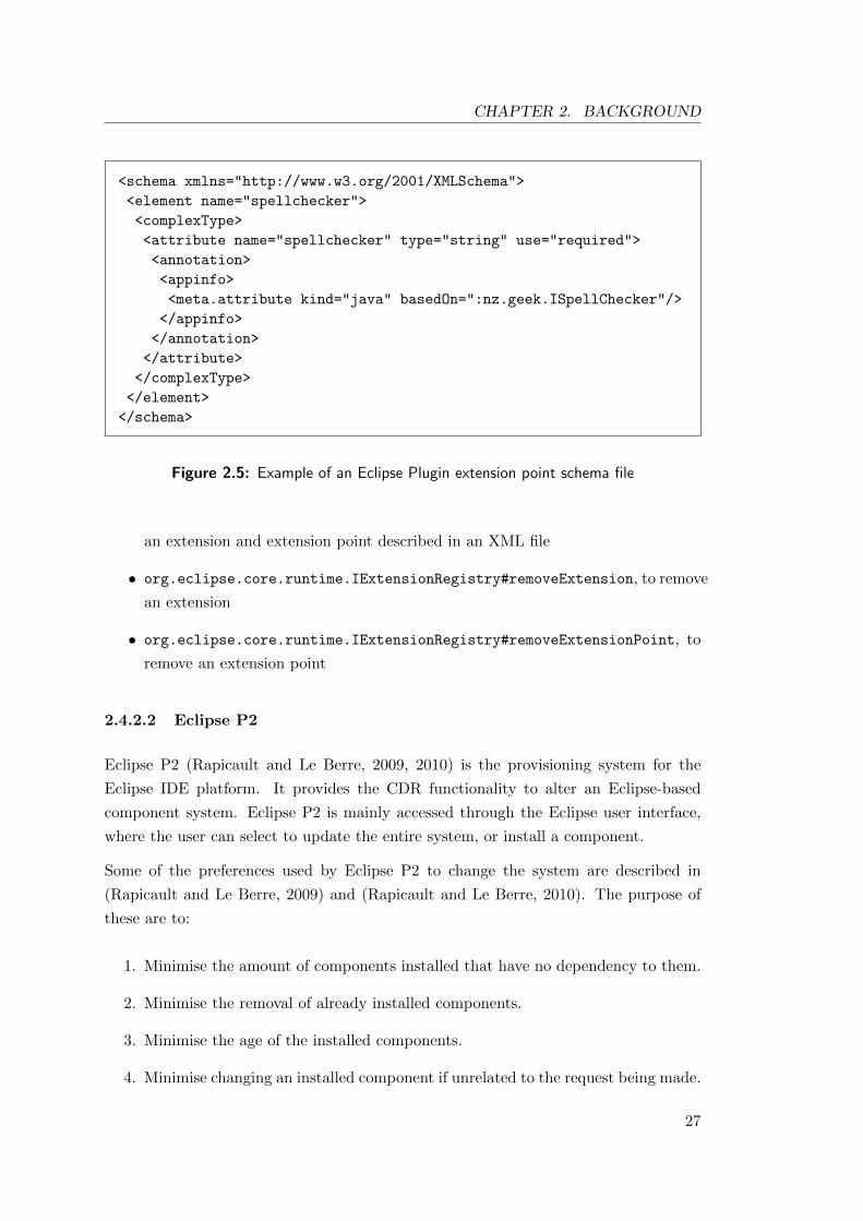
CHAPTER 2. BACKGROUND
<schema xmlns="http://www.w3.org/2001/XMLSchema">
<element name="spellchecker">
<complexType>
<attribute name="spellchecker" type="string" use="required">
<annotation>
<appinfo>
<meta.attribute kind="java" basedOn=":nz.geek.ISpellChecker"/>
</appinfo>
</annotation>
</attribute>
</complexType>
</element>
</schema>
Figure 2.5: Example of an Eclipse Plugin extension point schema file
an extension and extension point described in an XML file
• org.eclipse.core.runtime.IExtensionRegistry#removeExtension, to remove
an extension
• org.eclipse.core.runtime.IExtensionRegistry#removeExtensionPoint, to
remove an extension point
2.4.2.2 Eclipse P2
Eclipse P2 (Rapicault and Le Berre, 2009, 2010) is the provisioning system for the
Eclipse IDE platform. It provides the CDR functionality to alter an Eclipse-based
component system. Eclipse P2 is mainly accessed through the Eclipse user interface,
where the user can select to update the entire system, or install a component.
Some of the preferences used by Eclipse P2 to change the system are described in
(Rapicault and Le Berre, 2009) and (Rapicault and Le Berre, 2010). The purpose of
these are to:
1. Minimise the amount of components installed that have no dependency to them.
2. Minimise the removal of already installed components.
3. Minimise the age of the installed components.
4. Minimise changing an installed component if unrelated to the request being made.
27
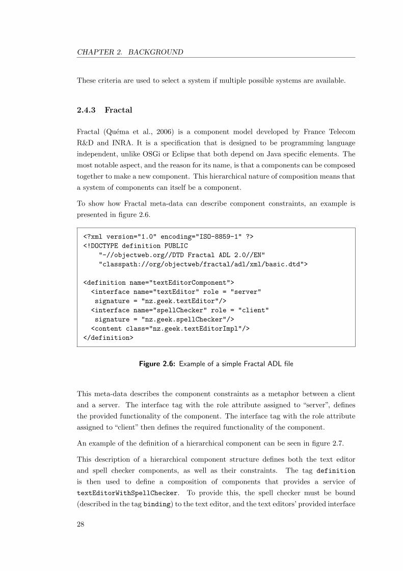
CHAPTER 2. BACKGROUND
These criteria are used to select a system if multiple possible systems are available.
2.4.3 Fractal
Fractal (Quema et al., 2006) is a component model developed by France Telecom
R&D and INRA. It is a specification that is designed to be programming language
independent, unlike OSGi or Eclipse that both depend on Java specific elements. The
most notable aspect, and the reason for its name, is that a components can be composed
together to make a new component. This hierarchical nature of composition means that
a system of components can itself be a component.
To show how Fractal meta-data can describe component constraints, an example is
presented in figure 2.6.
<?xml version="1.0" encoding="ISO-8859-1" ?>
<!DOCTYPE definition PUBLIC
"-//objectweb.org//DTD Fractal ADL 2.0//EN"
"classpath://org/objectweb/fractal/adl/xml/basic.dtd">
<definition name="textEditorComponent">
<interface name="textEditor" role = "server"
signature = "nz.geek.textEditor"/>
<interface name="spellChecker" role = "client"
signature = "nz.geek.spellChecker"/>
<content class="nz.geek.textEditorImpl"/>
</definition>
Figure 2.6: Example of a simple Fractal ADL file
This meta-data describes the component constraints as a metaphor between a client
and a server. The interface tag with the role attribute assigned to “server”, defines
the provided functionality of the component. The interface tag with the role attribute
assigned to “client” then defines the required functionality of the component.
An example of the definition of a hierarchical component can be seen in figure 2.7.
This description of a hierarchical component structure defines both the text editor
and spell checker components, as well as their constraints. The tag definition
is then used to define a composition of components that provides a service of
textEditorWithSpellChecker. To provide this, the spell checker must be bound
(described in the tag binding) to the text editor, and the text editors’ provided interface
28
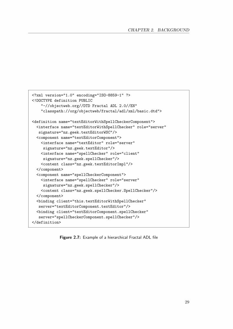
CHAPTER 2. BACKGROUND
<?xml version="1.0" encoding="ISO-8859-1" ?>
<!DOCTYPE definition PUBLIC
"-//objectweb.org//DTD Fractal ADL 2.0//EN"
"classpath://org/objectweb/fractal/adl/xml/basic.dtd">
<definition name="textEditorWithSpellCheckerComponent">
<interface name="textEditorWithSpellChecker" role="server"
signature="nz.geek.textEditorWSC"/>
<component name="textEditorComponent">
<interface name="textEditor" role="server"
signature="nz.geek.textEditor"/>
<interface name="spellChecker" role="client"
signature="nz.geek.spellChecker"/>
<content class="nz.geek.textEditorImpl"/>
</component>
<component name="spellCheckerComponent">
<interface name="spellChecker" role="server"
signature="nz.geek.spellChecker"/>
<content class="nz.geek.spellChecker.SpellChecker"/>
</component>
<binding client="this.textEditorWithSpellChecker"
server="textEditorComponent.textEditor"/>
<binding client="textEditorComponent.spellChecker"
server="spellCheckerComponent.spellChecker"/>
</definition>
Figure 2.7: Example of a hierarchical Fractal ADL file
29
CHAPTER 2. BACKGROUND
must be bound to the output interface.
2.4.3.1 Fractal Change
The programmatic evolution of a Fractal component system can differ between
implementations. To simplify this, only the Java implementation is described. In
this implementation the methods to edit the composition are9 (each interface is in the
package org.objectweb.fractal.api):
• To create a component:
factory.GenericFactory#newFcInstance.
• To add a component to a composite:
api.control.ContentController#addFcSubComponent.
• To remove a component from a composite:
control.ContentController#removeFcSubComponent.
There are two points that may make the changing a Fractal component model
particularly difficult: the hierarchical nature of Fractal, and the lack of required version
information about components and composites.
The hierarchical nature of Fractal will make it difficult to change a system. Given the
hierarchical nature of the components described, any system may provide the same
functionality with the same components in a combinatorial number of configurations.
When changing a system, not only would a new system need to be selected, but
components must be grouped to make composites. The simplest solution to this
problem is to ignore the hierarchical nature of this component model and have the
changed component system be exactly one composite with all components in it. More
difficult solutions could be created by reusing user composites, or analyzing the graph
structure to extract relationships by using algorithms like the one presented in (Dietrich
et al., 2008). This is not be explored in this research.
Another aspect that will make changing Fractal systems difficult, is the lack of
versioning information. Like OSGI-DS, this component model does not explicitly
require the version of the component and the interfaces they provide. This may lead
to problems as components and services evolve, and the dependencies on them cannot
specify which component version to depend on.
9http://fractal.ow2.org/current/doc/javadoc/fractal/ accessed 6/3/2012
30
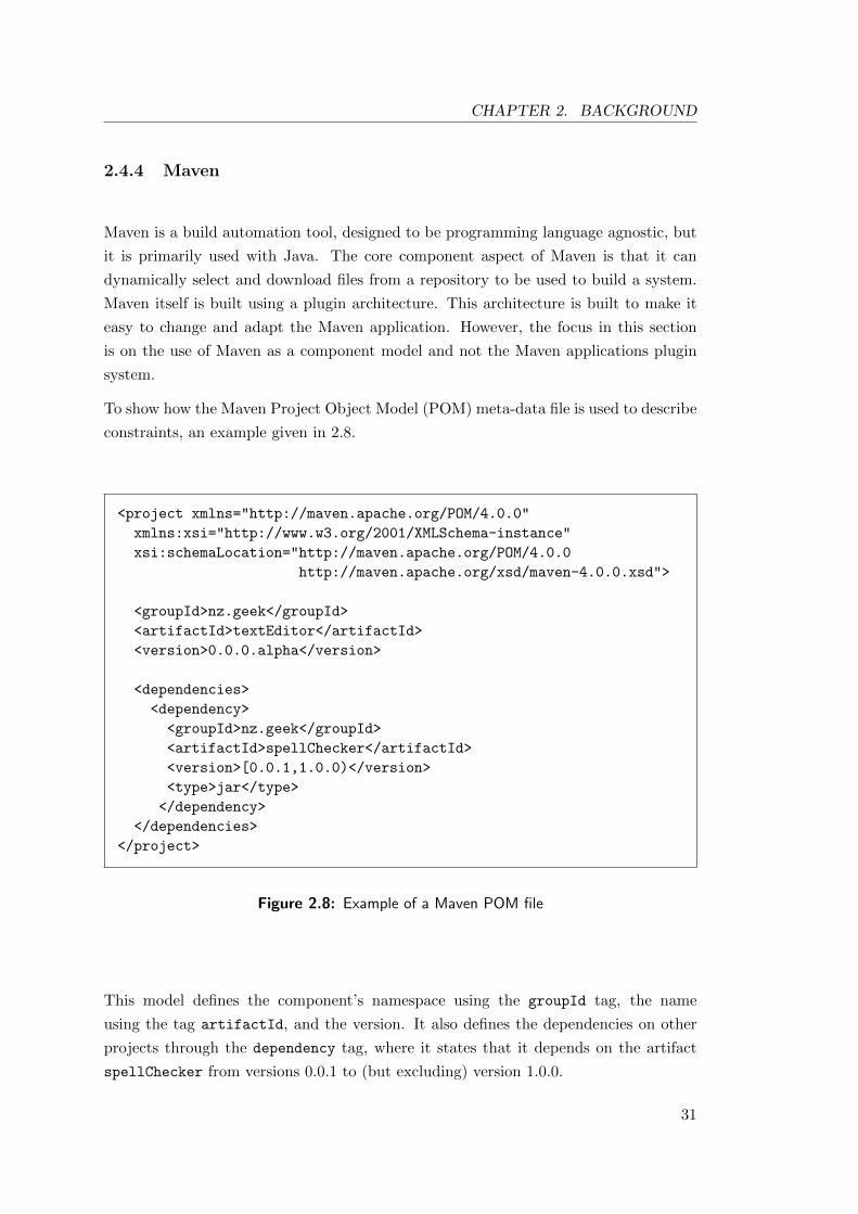
CHAPTER 2. BACKGROUND
2.4.4 Maven
Maven is a build automation tool, designed to be programming language agnostic, but
it is primarily used with Java. The core component aspect of Maven is that it can
dynamically select and download files from a repository to be used to build a system.
Maven itself is built using a plugin architecture. This architecture is built to make it
easy to change and adapt the Maven application. However, the focus in this section
is on the use of Maven as a component model and not the Maven applications plugin
system.
To show how the Maven Project Object Model (POM) meta-data file is used to describe
constraints, an example given in 2.8.
<project xmlns="http://maven.apache.org/POM/4.0.0"
xmlns:xsi="http://www.w3.org/2001/XMLSchema-instance"
xsi:schemaLocation="http://maven.apache.org/POM/4.0.0
http://maven.apache.org/xsd/maven-4.0.0.xsd">
<groupId>nz.geek</groupId>
<artifactId>textEditor</artifactId>
<version>0.0.0.alpha</version>
<dependencies>
<dependency>
<groupId>nz.geek</groupId>
<artifactId>spellChecker</artifactId>
<version>[0.0.1,1.0.0)</version>
<type>jar</type>
</dependency>
</dependencies>
</project>
Figure 2.8: Example of a Maven POM file
This model defines the component’s namespace using the groupId tag, the name
using the tag artifactId, and the version. It also defines the dependencies on other
projects through the dependency tag, where it states that it depends on the artifact
spellChecker from versions 0.0.1 to (but excluding) version 1.0.0.
31
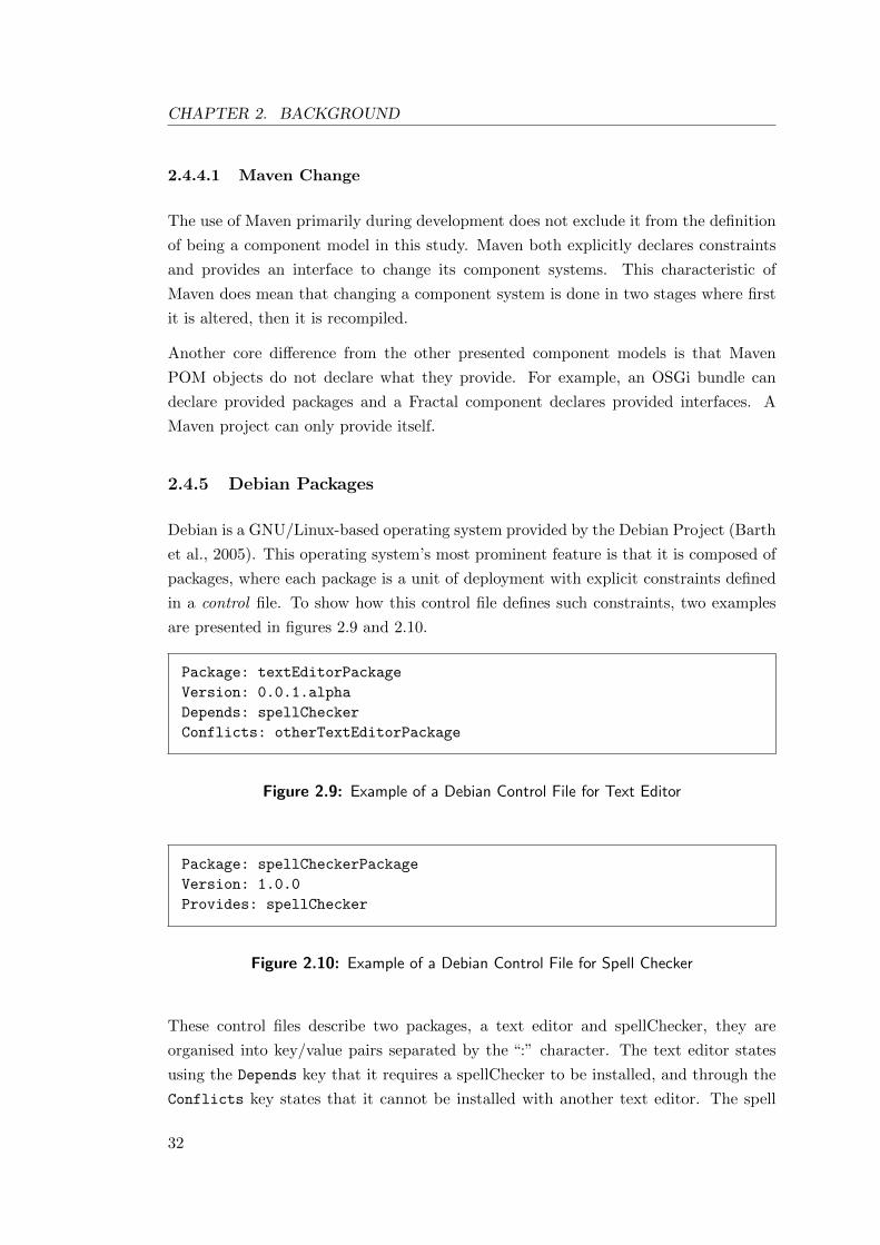
CHAPTER 2. BACKGROUND
2.4.4.1 Maven Change
The use of Maven primarily during development does not exclude it from the definition
of being a component model in this study. Maven both explicitly declares constraints
and provides an interface to change its component systems. This characteristic of
Maven does mean that changing a component system is done in two stages where first
it is altered, then it is recompiled.
Another core difference from the other presented component models is that Maven
POM objects do not declare what they provide. For example, an OSGi bundle can
declare provided packages and a Fractal component declares provided interfaces. A
Maven project can only provide itself.
2.4.5 Debian Packages
Debian is a GNU/Linux-based operating system provided by the Debian Project (Barth
et al., 2005). This operating system’s most prominent feature is that it is composed of
packages, where each package is a unit of deployment with explicit constraints defined
in a control file. To show how this control file defines such constraints, two examples
are presented in figures 2.9 and 2.10.
Package: textEditorPackage
Version: 0.0.1.alpha
Depends: spellChecker
Conflicts: otherTextEditorPackage
Figure 2.9: Example of a Debian Control File for Text Editor
Package: spellCheckerPackage
Version: 1.0.0
Provides: spellChecker
Figure 2.10: Example of a Debian Control File for Spell Checker
These control files describe two packages, a text editor and spellChecker, they are
organised into key/value pairs separated by the “:” character. The text editor states
using the Depends key that it requires a spellChecker to be installed, and through the
Conflicts key states that it cannot be installed with another text editor. The spell
32
CHAPTER 2. BACKGROUND
checker package defines that it provides a spell checker using the Provides key. This
spell checker is of a type called a virtual package, which has some specific semantics
not described here.
One aspect that differentiates the Debian package model from the many other models, is
that it does not specify the rules of composition between components. That is, there is
no formal specification of the semantics of the communication and relationships between
packages. For instance, OSGi bundles exist in a very constrained environment that
manages their interactions, depending on another bundle has run-time implications.
For Debian, the dependence of one package on another has no prescribed run-time
effects, other than the assumption that without satisfying the dependence the package
will not be functional. The way in which a package uses or communicates with a
depended upon package is defined between the packages and not in the component
model.
2.4.5.1 dpkg
The application dpkg is the command line tool use to modify a Debian package system.
The commands to modify a Debian package system are:
• To add a package: dpkg -install <package file>.
• To remove a package: dpkg -remove <package>.
These commands define the atomic actions to change a Debian system. They can
be executed from other applications through the command line, this makes them
programming language independent and easily accessible.
2.4.5.2 apt-get
The dpkg application can only remove and add a single component at a time, it does
not satisfy the constraints of a component. There are many applications that provide
CDR functionality on Debian systems, the default and most popular solution is through
the apt-get application. This tool is built on top of dpkg, to provide an interface to
simplify and extend its functionality. The apt-get application is a command line tool,
which provides the necessary tools to efficiently allow the user to evolve their system.
apt-get follows some basic criteria when altering the system. For example, when
upgrading:
33
CHAPTER 2. BACKGROUND
• Under no circumstances will apt-get remove an already installed package.
• Under no circumstances will apt-get install a new package.
Note: apt-get defines removing, installing and upgrading separately, e.g. upgrading a
package named text-editor is not defined by apt-get as removing then installing a
new package.
Another application that extends apt-get’s functionality is aptitude (Burrows, 2005).
This application adds a basic user interface to apt-get and also extends functionality
in aspects like locating and removing redundant packages. Aptitude allows some of its
criteria to be user defined, for example when the flag --safe-resolver is used:
• It attempts to preserve as many of your choices as possible.
• It will never remove a package.
• It will never install a version of a package other than the package’s default
candidate version.
2.4.6 SOFA 2.0
Software Appliance (SOFA) (Hnetynka and Plasil, 2006) is a component model
developed at Charles University in Prague. A component in the SOFA framework
is defined by it’s frame, which contains the meta-data of what the component requires
and provides. Like Fractal, SOFA is a hierarchical component model, allowing for a
composite of components to be treated as a single component.
To show how SOFA meta-data describes constraints an example is presented in figure
2.11.
This meta-data describes two components, a text editor and a spell checker,
using the tag frame. The sub elements requires and provides describe the
component constraints through an externally defined interface with the name-space
sofatype://nz.geek.spellChecker.
2.4.6.1 SOFA Change
SOFA 2.0 is an extension of the SOFA framework, with new services including dynamic
reconfiguration for dynamic evolution of an architecture at run-time. Unlike other
component systems, it only allows for controlled change; many component models
34
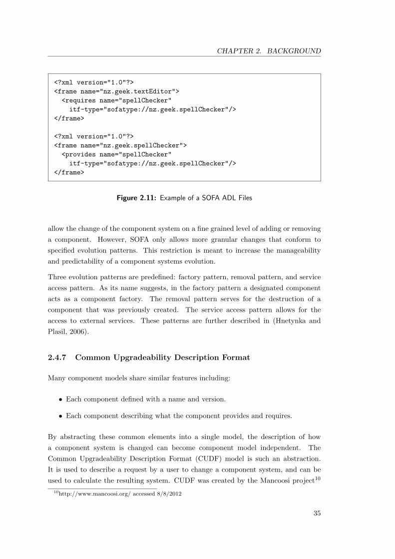
CHAPTER 2. BACKGROUND
<?xml version="1.0"?>
<frame name="nz.geek.textEditor">
<requires name="spellChecker"
itf-type="sofatype://nz.geek.spellChecker"/>
</frame>
<?xml version="1.0"?>
<frame name="nz.geek.spellChecker">
<provides name="spellChecker"
itf-type="sofatype://nz.geek.spellChecker"/>
</frame>
Figure 2.11: Example of a SOFA ADL Files
allow the change of the component system on a fine grained level of adding or removing
a component. However, SOFA only allows more granular changes that conform to
specified evolution patterns. This restriction is meant to increase the manageability
and predictability of a component systems evolution.
Three evolution patterns are predefined: factory pattern, removal pattern, and service
access pattern. As its name suggests, in the factory pattern a designated component
acts as a component factory. The removal pattern serves for the destruction of a
component that was previously created. The service access pattern allows for the
access to external services. These patterns are further described in (Hnetynka and
Plasil, 2006).
2.4.7 Common Upgradeability Description Format
Many component models share similar features including:
• Each component defined with a name and version.
• Each component describing what the component provides and requires.
By abstracting these common elements into a single model, the description of how
a component system is changed can become component model independent. The
Common Upgradeability Description Format (CUDF) model is such an abstraction.
It is used to describe a request by a user to change a component system, and can be
used to calculate the resulting system. CUDF was created by the Mancoosi project10
10http://www.mancoosi.org/ accessed 8/8/2012
35
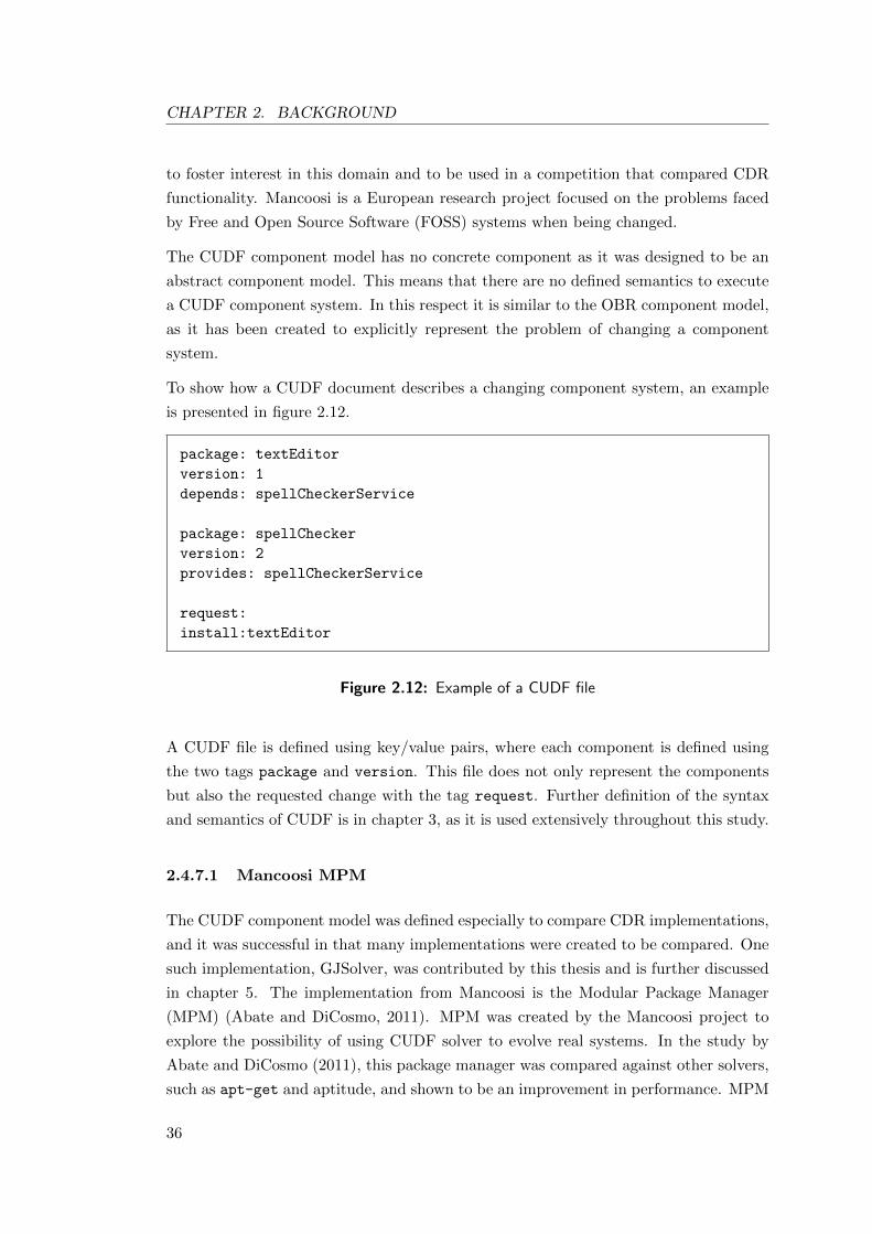
CHAPTER 2. BACKGROUND
to foster interest in this domain and to be used in a competition that compared CDR
functionality. Mancoosi is a European research project focused on the problems faced
by Free and Open Source Software (FOSS) systems when being changed.
The CUDF component model has no concrete component as it was designed to be an
abstract component model. This means that there are no defined semantics to execute
a CUDF component system. In this respect it is similar to the OBR component model,
as it has been created to explicitly represent the problem of changing a component
system.
To show how a CUDF document describes a changing component system, an example
is presented in figure 2.12.
package: textEditor
version: 1
depends: spellCheckerService
package: spellChecker
version: 2
provides: spellCheckerService
request:
install:textEditor
Figure 2.12: Example of a CUDF file
A CUDF file is defined using key/value pairs, where each component is defined using
the two tags package and version. This file does not only represent the components
but also the requested change with the tag request. Further definition of the syntax
and semantics of CUDF is in chapter 3, as it is used extensively throughout this study.
2.4.7.1 Mancoosi MPM
The CUDF component model was defined especially to compare CDR implementations,
and it was successful in that many implementations were created to be compared. One
such implementation, GJSolver, was contributed by this thesis and is further discussed
in chapter 5. The implementation from Mancoosi is the Modular Package Manager
(MPM) (Abate and DiCosmo, 2011). MPM was created by the Mancoosi project to
explore the possibility of using CUDF solver to evolve real systems. In the study by
Abate and DiCosmo (2011), this package manager was compared against other solvers,
such as apt-get and aptitude, and shown to be an improvement in performance. MPM
36
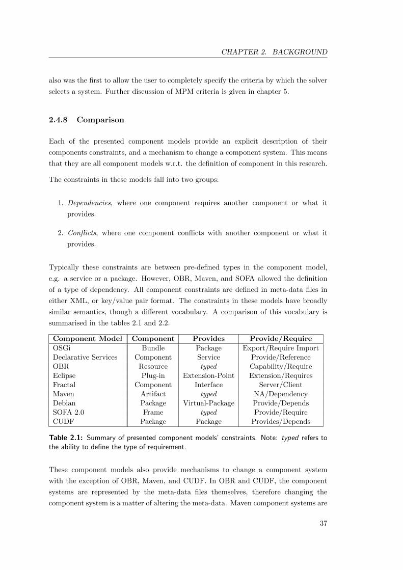
CHAPTER 2. BACKGROUND
also was the first to allow the user to completely specify the criteria by which the solver
selects a system. Further discussion of MPM criteria is given in chapter 5.
2.4.8 Comparison
Each of the presented component models provide an explicit description of their
components constraints, and a mechanism to change a component system. This means
that they are all component models w.r.t. the definition of component in this research.
The constraints in these models fall into two groups:
1. Dependencies, where one component requires another component or what it
provides.
2. Conflicts, where one component conflicts with another component or what it
provides.
Typically these constraints are between pre-defined types in the component model,
e.g. a service or a package. However, OBR, Maven, and SOFA allowed the definition
of a type of dependency. All component constraints are defined in meta-data files in
either XML, or key/value pair format. The constraints in these models have broadly
similar semantics, though a different vocabulary. A comparison of this vocabulary is
summarised in the tables 2.1 and 2.2.
Component Model Component Provides Provide/Require
OSGi Bundle Package Export/Require ImportDeclarative Services Component Service Provide/ReferenceOBR Resource typed Capability/RequireEclipse Plug-in Extension-Point Extension/RequiresFractal Component Interface Server/ClientMaven Artifact typed NA/DependencyDebian Package Virtual-Package Provide/DependsSOFA 2.0 Frame typed Provide/RequireCUDF Package Package Provides/Depends
Table 2.1: Summary of presented component models’ constraints. Note: typed refers tothe ability to define the type of requirement.
These component models also provide mechanisms to change a component system
with the exception of OBR, Maven, and CUDF. In OBR and CUDF, the component
systems are represented by the meta-data files themselves, therefore changing the
component system is a matter of altering the meta-data. Maven component systems are
37
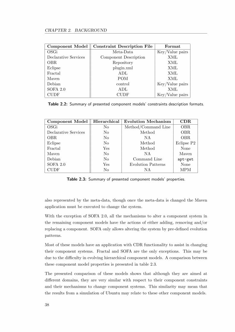
CHAPTER 2. BACKGROUND
Component Model Constraint Description File Format
OSGi Meta-Data Key/Value pairsDeclarative Services Component Description XMLOBR Repository XMLEclipse plugin.xml XMLFractal ADL XMLMaven POM XMLDebian control Key/Value pairsSOFA 2.0 ADL XMLCUDF CUDF Key/Value pairs
Table 2.2: Summary of presented component models’ constraints description formats.
Component Model Hierarchical Evolution Mechanism CDR
OSGi No Method/Command Line OBRDeclarative Services No Method OBROBR No NA OBREclipse No Method Eclipse P2Fractal Yes Method NoneMaven No NA MavenDebian No Command Line apt-get
SOFA 2.0 Yes Evolution Patterns NoneCUDF No NA MPM
Table 2.3: Summary of presented component models’ properties.
also represented by the meta-data, though once the meta-data is changed the Maven
application must be executed to change the system.
With the exception of SOFA 2.0, all the mechanisms to alter a component system in
the remaining component models have the actions of either adding, removing and/or
replacing a component. SOFA only allows altering the system by pre-defined evolution
patterns.
Most of these models have an application with CDR functionality to assist in changing
their component systems. Fractal and SOFA are the only exceptions. This may be
due to the difficulty in evolving hierarchical component models. A comparison between
these component model properties is presented in table 2.3.
The presented comparison of these models shows that although they are aimed at
different domains, they are very similar with respect to their component constraints
and their mechanisms to change component systems. This similarity may mean that
the results from a simulation of Ubuntu may relate to these other component models.
38
CHAPTER 2. BACKGROUND
2.5 Summary
In this chapter, the concepts related to CSE are explored. The domains of software
evolution, CBSE and component systems are described and the important concepts,
such as software component, are defined. Various component models are described,
and it was shown that there exist no fundamental differences between these models.
Therefore, a single model can be used to describe the evolution of component systems
conforming to these various models. In the next chapter a model that formally defines
the concepts discussed in this chapter is presented. This is the first step towards creating
a simulation of CSE.
39
CHAPTER 2. BACKGROUND
40
Chapter 3
Formal Model of Component
System Evolution
We are like sailors who on the open sea must reconstruct their ship but are never
able to start afresh from the bottom.Willard Van Orman Quine, Word and Object, 1960
In the previous chapter, component system evolution (CSE) was described as the
continual alteration of a system of components by a composer. The described
component models each defined constraints on this change to ensure the resulting
system is valid.
This chapter describes the model (CoSyE) and language (CUDF*) used to describe the
CSE process. They also enable the discussion of CSE as they formally define terms and
concepts used in this research.
The model CoSyE (Component System Evolution) aims for the qualities of a model
described by Selic (2003):
• Abstractness: A model is a reduction of reality, removing or hiding detail that
is irrelevant.
• Understandability: A model directly appeals to intuition, to convey complex
ideas with little intellectual effort.
• Accuracy: A model must provide a true to life representation of the modelled
system.
• Predictiveness: A model must be able to be used to predict the modelled
system’s non-obvious yet interesting properties.
41
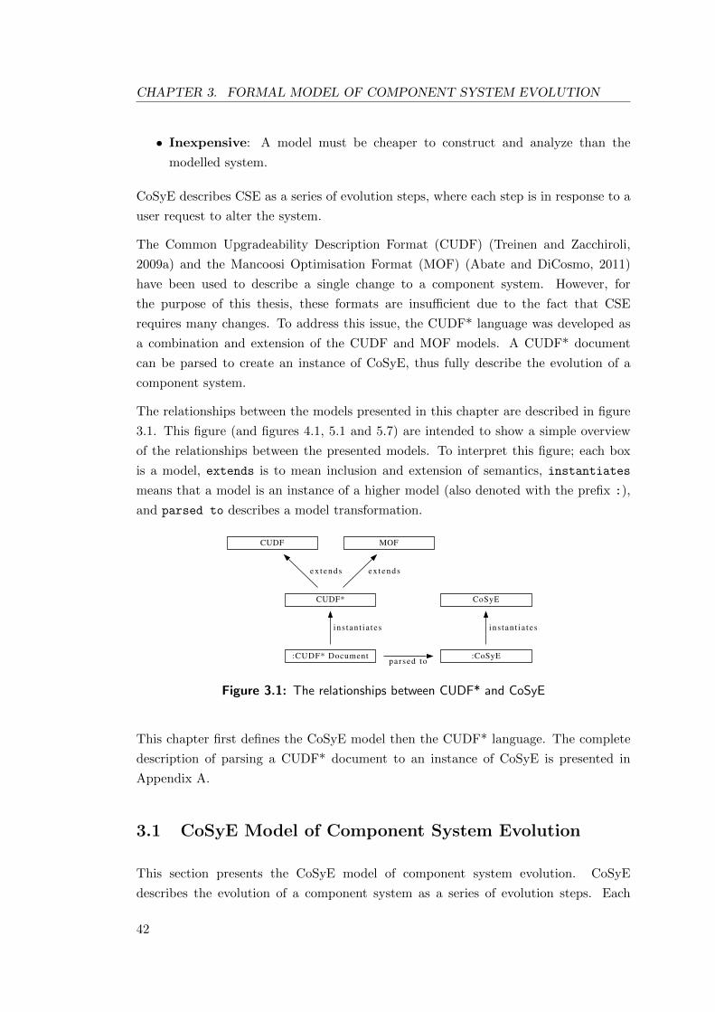
CHAPTER 3. FORMAL MODEL OF COMPONENT SYSTEM EVOLUTION
• Inexpensive: A model must be cheaper to construct and analyze than the
modelled system.
CoSyE describes CSE as a series of evolution steps, where each step is in response to a
user request to alter the system.
The Common Upgradeability Description Format (CUDF) (Treinen and Zacchiroli,
2009a) and the Mancoosi Optimisation Format (MOF) (Abate and DiCosmo, 2011)
have been used to describe a single change to a component system. However, for
the purpose of this thesis, these formats are insufficient due to the fact that CSE
requires many changes. To address this issue, the CUDF* language was developed as
a combination and extension of the CUDF and MOF models. A CUDF* document
can be parsed to create an instance of CoSyE, thus fully describe the evolution of a
component system.
The relationships between the models presented in this chapter are described in figure
3.1. This figure (and figures 4.1, 5.1 and 5.7) are intended to show a simple overview
of the relationships between the presented models. To interpret this figure; each box
is a model, extends is to mean inclusion and extension of semantics, instantiates
means that a model is an instance of a higher model (also denoted with the prefix :),
and parsed to describes a model transformation.
CoSyE
:CoSyE
ins tan t ia tes
CUDF MOF
CUDF*
ex t ends ex t ends
:CUDF* Documentparsed to
ins tan t ia tes
Figure 3.1: The relationships between CUDF* and CoSyE
This chapter first defines the CoSyE model then the CUDF* language. The complete
description of parsing a CUDF* document to an instance of CoSyE is presented in
Appendix A.
3.1 CoSyE Model of Component System Evolution
This section presents the CoSyE model of component system evolution. CoSyE
describes the evolution of a component system as a series of evolution steps. Each
42
CHAPTER 3. FORMAL MODEL OF COMPONENT SYSTEM EVOLUTION
step tries to satisfy a user request for change along with the constraints that ensure the
system is valid. The selected component system is optimal with respect to a preference
order.
3.1.1 Evolution Problem
The solutions to an evolution problem make up the set of valid component systems
that can be evolved to. To define this, first the basic elements of the model must be
defined, such as components and constraints.
Components are the atomic units of a component system’s evolution.
Definition 1 Let N be the set of names, where a name is a finite string of characters;
let V be the totally ordered set of versions1; a component is an element of C, where
C = N × V.
A component a is then a pair 〈n, v〉, where n is the component’s name, and v is
the component’s version. The characters a, b, c, . . . are used to denote components,
m,n, o, . . . used to denote names, and v, w, x, . . . used to denote versions.
Definition 2 A component system is a finite subset of components, e.g. α is a
component system where α ⊆finite C.
The characters α, β, γ are used to denote component systems2.
Constraints are used to describe valid systems.
Definition 3 A constraint con is a set of component systems, i.e. con ⊆ 2C.
Such constraints can be defined intentionally by specifying the necessary and sufficient
conditions for a component system to be in a constraint.
In most component models described in chapter 2, only specific types of constraints are
used, these types are:
1. Exclusion: ¬a := α ∈ 2C | a 6∈ α .
1Given V is ordered under ≤, ≤ is antisymmetric (v ≤ w and w ≤ v then v = w), transitive (v ≤ wand w ≤ x then v ≤ x) and total (v ≤ w or w ≤ v)
2In hierarchical component models, such as Fractal (Quema et al., 2006), a component system wouldalso be a component. That is, a component system could have elements that are themselves componentsystems. This definition is not included in this model, though it may be possible for it to be modifiedto include it in the future.
43
CHAPTER 3. FORMAL MODEL OF COMPONENT SYSTEM EVOLUTION
2. Conflict: a→ ¬c := α ∈ 2C | if a ∈ α then c 6∈ α .
3. Inclusive Disjunction: a1 ∨ . . . ∨ an := α ∈ 2C | a1 ∈ α or . . . or an ∈ α .
4. Dependence: a→ c1∨ . . .∨ cn := α ∈ 2C | if a1 ∈ α then c1 ∈ α or . . . or cn ∈α .
5. Exactly One: a1 + . . .+ an = 1 := α ∈ 2C | |a1, . . . , an ∩ α| = 1 .
Note, for constraint types 3, 4 and 5 the value of n can be equal to 1.
The vocabulary used when discussing constraints is as follows:
Definition 4
1. A component system α is said to satisfy a constraint con iff α ∈ con.
2. An evolution problem EP is a finite set of constraints.
3. A solution to an evolution problem EP is a component system α that satisfies
all constraints in the evolution problem, i.e. α ∈ coni for all coni ∈ EP .
4. An evolution problem is unsatisfiable if there exists no solution to it.
Based on the definitions presented in this section, the following example illustrates how
an evolution problem can be described and solved. Assume the evolution problem EP
is defined as the set of two constraints con1 and con2, i.e. EP = con1, con2. The
constraint con1 is b (constraint type 3), which is defined as the set of all component
systems with b in them. The constraint con2 is a → c (constraint type 4), is defined
as the set of all component systems where if a is included, then c is included. The
component systems that satisfy both con1 and con2 are solutions to EP . Some of these
solutions are b, a, b, c and a, b, c, d.
3.1.1.1 Complexity of an Evolution Problem
When investigating the complexity of an evolution problem, it was observed that:
Observation 1 Finding a solution to an evolution problem is NP-complete (Cook,
1971).
This observation has been made before by Mancinelli et al. (2006) and Abate and
DiCosmo (2011). This can be shown by reducing a known NP-complete problem, called
one-in-three satisfiability, to the evolution problem. The one-in-three satisfiability
problem is defined by Schaefer (1978) as:
44

CHAPTER 3. FORMAL MODEL OF COMPONENT SYSTEM EVOLUTION
Given sets S1, . . . , Sn each having at most 3 members, is there a subset T
of the members such that for each i, |T ∩ Si| = 1.
This can be reduced to an evolution problem where:
Given sets S1, . . . , Sn each containing 3 components, and constraints
con1, . . . , conn such that for each i, Si = a, b, c iff coni equals constraint
a + b + c = 1 (constraint type 5). A set of components α is such that
for each i, |α ∩ Si| = 1 iff α is a solution to the evolution problem
EP = con1, . . . , conn.
This reduction uses the “exactly one” constraint (type 5). However, if this constraint
type was not included into this formalism, the evolution problem would still be NP-
Complete, as one-in-three satisfiability can be reduced to a problem consisting of
constraint types 2 and 3.
3.1.2 Constraints and Requests
An evolution problem consists of two sets of constraints; constraints created by the user
request to change the system, and constraints required for the system to be valid. To
clarify the purpose of these constraints, they are separated into two sets.
Definition 5 The set of user requests ∆ is the set of all constraints, where each
constraint in ∆ is either:
1. an installation request of constraint type 3.
2. a remove request of constraint type 1.
3. a *grade3 request of constraint type 5.
Consider the examples of:
• an installation request a ∨ b is a request by the user to install component a or b
into the system.
• a remove request ¬a is a request by the user to remove component a from the
system.
3This referrers to either request an upgrade or a downgrade
45
CHAPTER 3. FORMAL MODEL OF COMPONENT SYSTEM EVOLUTION
• a *grade request a + b = 1 is a request by the user to include either a or b, but
not both.
The *grade request uses the “exactly one” constraint (type 5) to represent both
downgrade and upgrade requests from the user. The intuition is that after upgrading
or downgrading a component, exactly one component should be included in the system
(Treinen and Zacchiroli, 2009a).
Definition 6 The set of system constraints Ω is a set of all constraints, where each
constraint in Ω is either:
1. a keep constraint of type 3.
2. a dependency constraint of type 4.
3. a conflict constraint of type 2.
Consider the examples of:
• a keep constraint a ∨ b is a system constraint to keep component a or b in the
system.
• a dependency constraint a → b ∨ c is a system constraint where if a is in the
system, then b or c must be in the system.
• a conflict constraint a → ¬b is a system constraint where if a is in the system
then b must not be in the system.
The evolution of a component system happens over time. This concept of “time” must
be introduced to the model.
Definition 7 The set T is the set of all times. T is a strict total ordered under <time,
where times ti and ti+1 in T implies ti <time ti+1
At any time, there exists only a finite set of components.
Definition 8 Ct is the finite set of components that exists at time t, Ct ⊂finite C
At any point in time, the sets of system constraints and user request constraints are
with respect to the set of components that exist at that time. That is, a constraint can
only describe systems that are composed of components that exist at a given time.
46
CHAPTER 3. FORMAL MODEL OF COMPONENT SYSTEM EVOLUTION
Definition 9 Given time t, and the set of components Ct, the set of system
constraints w.r.t. time is Ωt, where Ωt = con ∩ 2Ct | con ∈ Ω, and the set of
user requests w.r.t. time is ∆t, where ∆t = con ∩ 2Ct | con ∈ ∆
Definition 10 Given a time t, a user request, δt, is a finite set of user requests at
time t, i.e. δt ⊆finite ∆t; and a set of system constraints, ωt, is a finite set of system
constraints at time t, i.e. ωt ⊆finite Ωt.
An evolution problem, EP , can be defined by combining a user request δt and a set of
system constraints ωt, such that EP = δt ∪ ωt.
An example is presented to illustrate the relationship an evolution problem has to
time. Consider the system constraint con1 that is defined as a → b ∨ d, and the user
request constraint con2 defined as a (a singleton installation constraint). The constraint
con1 can (but is not limited to) be satisfied by the component systems , b, a, b,a, b, d, and a, d, and the constraint con2 can (but is not limited to) be satisfied by
component systems a, a, b and a, b, d.
Assume that at time t, only the components a and b exist, i.e Ct = a, b. The set
of all component systems at time t is 2Ct = , a, b, a, b. Therefore, at time t
component d does not exist, it is not in Ct, nor in any component system in 2Ct .
The system constraint con′1 ∈ Ωt, is such that con′1 = con1 ∩ 2Ct = , b, a, b.The user request constraint con′2 ∈ ∆t, is such that con′2 = con2 ∩ 2Ct = a, a, b.
Assume a set of system constraints ωt = con′1, and a user request constraints
δt = con′2. An evolution problem δt∪ωt, will have exactly one solution, the component
system a, b.
3.1.3 Component System Evolution
A component system is changed from one system to another to satisfy an evolution
problem containing a user request and system constraints. Many evolution problems
have multiple valid solutions, as evolution problems are generally under-constrained
(Le Berre and Parrain, 2008). Different solutions may have different properties, and as
a result, a user may prefer one system over another. Introducing an ordering over the
solutions addresses such user preferences.
Definition 11 Given a component system α, an evolution preference order w.r.t.
α is a strict partial order ≺α⊆ 2C × 2C.
47
CHAPTER 3. FORMAL MODEL OF COMPONENT SYSTEM EVOLUTION
A strict partial order has the properties of irreflexivity (not β ≺α β), asymmetry (if
β ≺α β′ then not β′ ≺α β), and transitivity (if β ≺α β′ and β′ ≺α β′′ then β ≺α β′′).The non-strict evolution preference order α can be defined such that β ≺α β′ if and
only if (β α β′ and β 6= β′).
Definition 12 Given a component system α, an evolution preference order w.r.t. α
≺α, and an evolution problem EP ; a component system β is optimal if β is a solution
to EP , and there exists no other solution to EP β′, such that β ≺α β′.
Definition 13 Given times ti−1 and ti, a component system αti−1, an evolution
preference order ≺αti−1, a user request δti, and a set of system constraints ωti; the
evolution step function ε(αti−1 , δti ∪ωti) returns the component system αti such that:
• iff the evolution problem δti∪ωti is satisfiable, αti is an optimal solution to δti∪ωti.
• iff the evolution problem δti ∪ ωti is unsatisfiable, αti equals αti−1.
The evolution step function takes a previous system and changes it to satisfy a user’s
request and system constraints with a preferable system. If the evolution problem
is unsatisfiable, the evolution step function does not change the system and returns
the previous system αti−1 . Such a situation occurs when the user requests a change
that either conflicts with itself, or conflicts with the system constraints. For example,
consider the situation where a user requested to install components a and b, but a and b
conflict with each other. If this situation happened in reality, a report will be generated
and returned to the user explaining why the evolution problem is unsatisfiable. This
report may also include hints to the user as to how to make the request satisfiable.
If an evolution problem is unsatisfiable, it could be possible to return a component
system that maximises the number of satisfied constraints in the user request. This
approach, however, is impossible to define as the intentions of a user request are
unknown. For example, consider the situation where a user requested to install
components a and b, but a and b conflict with each other. Which component should
be selected to be installed in the system? Given the user request, this question cannot
be answered. The user may only require a if b is installed, or vice versa. Making no
assumptions about the intent of the user request is the prudent approach taken in this
model.
Definition 14 Given a series of times t0, . . . , tn, an initial component system αt0,
sets of components Ct1 , . . . , Ctn, a series of user requests δt1 , . . . , δtn, a series of system
48
CHAPTER 3. FORMAL MODEL OF COMPONENT SYSTEM EVOLUTION
constraints ωt1 , . . . , ωtn, and a series of evolution preference orders ≺αt0, . . . ,≺αtn−1
;
the evolution function ε∗ is defined as
ε∗(αt0 , 〈δt1 ∪ ωt1 , . . . , δtn ∪ ωtn〉) = ε(ε(. . . ε(αt0 , δt1 ∪ ωt1), . . .), δtn ∪ ωtn) = αtn.
This evolution function is the core definition in CoSyE as it describes the evolution
process of repeatedly changing a component system. That is, the evolution function ε∗
is the “closure” of the evolution step function ε. An instance of CoSyE will contain:
• A series of times t0, . . . , tn.
• Sets of components Ct0 , . . . ,Ctn .
• Sets of user requests δt1 , . . . , δtn .
• Sets of system constraints ωt1 , . . . , ωtn .
• Evolution preference orders ≺αt0, . . . ,≺αtn−1
.
• Initial system αt0 .
This is enough information to calculate the system from αt1 to αtn , also known as
resolving a CoSyE instance.
The following observations can be made about the CoSyE model.
Observation 2 It is not required for an evolution step to satisfy prior user requests.
For example, if a user wants to install a text editor into the system, the user would
expect that in future the text editor will remain in the system. This property is not
explicitly stated in the model, because (as described above) it is difficult to determine
a user’s intention with a request.
A similar problem is faced by the revision function in the domain of belief revision
(Alchourron et al., 1985). Revision functions try to preserve consistency across a set of
beliefs as new, and possibly inconsistent, information is introduced. This is similar, as a
set of previous user requests should try to remain satisfied with the component system,
as the user requests to change the system. This problem with the evolution process
is not further explored in this research, but belief revision may provide inspiration for
future research.
Observation 3 Multiple evolution steps may produce a less optimal component system
than an equivalent, single evolution step.
49
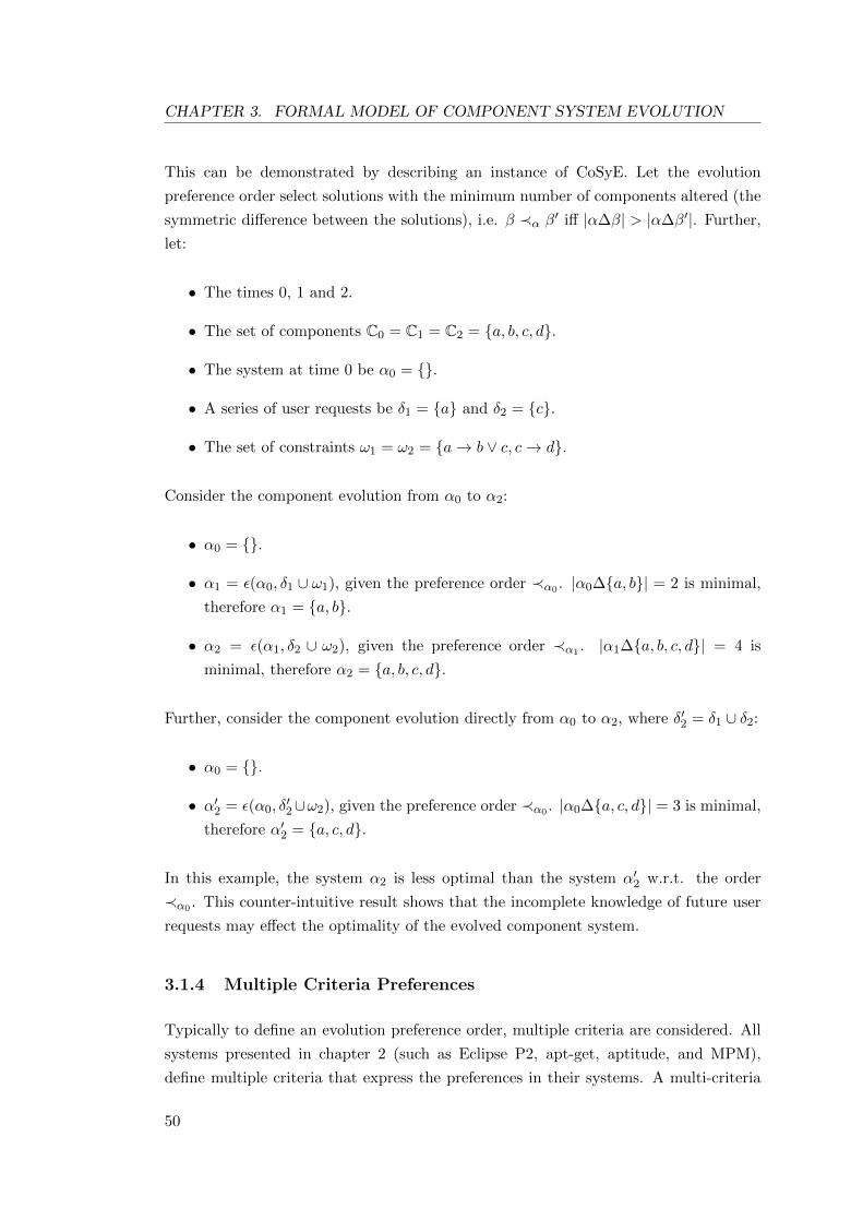
CHAPTER 3. FORMAL MODEL OF COMPONENT SYSTEM EVOLUTION
This can be demonstrated by describing an instance of CoSyE. Let the evolution
preference order select solutions with the minimum number of components altered (the
symmetric difference between the solutions), i.e. β ≺α β′ iff |α∆β| > |α∆β′|. Further,
let:
• The times 0, 1 and 2.
• The set of components C0 = C1 = C2 = a, b, c, d.
• The system at time 0 be α0 = .
• A series of user requests be δ1 = a and δ2 = c.
• The set of constraints ω1 = ω2 = a→ b ∨ c, c→ d.
Consider the component evolution from α0 to α2:
• α0 = .
• α1 = ε(α0, δ1 ∪ ω1), given the preference order ≺α0 . |α0∆a, b| = 2 is minimal,
therefore α1 = a, b.
• α2 = ε(α1, δ2 ∪ ω2), given the preference order ≺α1 . |α1∆a, b, c, d| = 4 is
minimal, therefore α2 = a, b, c, d.
Further, consider the component evolution directly from α0 to α2, where δ′2 = δ1 ∪ δ2:
• α0 = .
• α′2 = ε(α0, δ′2∪ω2), given the preference order ≺α0 . |α0∆a, c, d| = 3 is minimal,
therefore α′2 = a, c, d.
In this example, the system α2 is less optimal than the system α′2 w.r.t. the order
≺α0 . This counter-intuitive result shows that the incomplete knowledge of future user
requests may effect the optimality of the evolved component system.
3.1.4 Multiple Criteria Preferences
Typically to define an evolution preference order, multiple criteria are considered. All
systems presented in chapter 2 (such as Eclipse P2, apt-get, aptitude, and MPM),
define multiple criteria that express the preferences in their systems. A multi-criteria
50
CHAPTER 3. FORMAL MODEL OF COMPONENT SYSTEM EVOLUTION
framework is presented as part of CoSyE, to enable the description of evolution
preference orders.
A simple way to define the order ≺α, can be by defining a scoring function (f :
2C × 2C → R) for each criterion. These functions can then be aggregated, e.g. using
addition or multiplication (possibly with weights), and used to define ≺α. For example,
a function that returns the number of components that have changed between systems
is defined fchange(α, β) = |α∆β|. A function that returns the size of all components in
a component system is defined fsize(α, β) =∑c∈β
size(c), where size is a function that
takes a component and returns its size in kilobytes. The evolution preference order could
then be defined as β ≺α β′ iff fchange(α, β) + fsize(α, β) > fchange(α, β′) + fsize(α, β
′).
Defining the evolution preference order in this manner has some drawbacks:
• Information can be lost in the conversion to real numbers, e.g. the reason why a
specific system was selected over another.
• The relationships between criteria are difficult to intuitively define, e.g. “size +
change” results in a confusing metric.
• Altering weights to express order over criteria does not convey meaningful
information about decisions or their impact. For example, stating “the size of
a system is .25 multiplied by the change of a system” does not convey what the
implications of the weighting will be.
A possibly more intuitive approach to define the evolution preference order is to create
a ranking function that measures a component system against an arbitrary range. A
criterion is then a ranking function and an order over its range. By not reducing the
problem to only real numbers, information can be retained about the selection of a
component system.
Using a lexicographic order, each criterion can then be composed together into a
composite criterion. The lexicographic composition lets an order over the preference of
criteria be defined, without having to assign arbitrary weights. This method has been
used before in the MPM (Abate and DiCosmo, 2011). It is the selected mechanism to
define the preference order in this thesis.
Definition 15 A ranking function, rankα, is a function that ranks a component
system to a range A w.r.t. a component system α, i.e. rankα : 2C → A.
The range A could be real or natural numbers, integers, versions, components, . . .
51
CHAPTER 3. FORMAL MODEL OF COMPONENT SYSTEM EVOLUTION
Definition 16 A criterion is a tuple 〈rankα,≤〉, where the ranking function is defined
as rankα : 2C → A, and ≤ (whose strict order is <) is a partial order over A.
The order ≤ is a partial order; ≤ is reflexive (a ≤ a), antisymmetry (if a ≤ b and b ≤a then a = b), and transitive (if a ≤ b and b ≤ c then a ≤ c).
The evolution preference order is described with respect to a criterion.
Definition 17 The evolution preference order ≺α can be defined with a criterion
〈rankα,≤〉, such that given component systems β and β′, iff rankα(β) is strictly less
than (<) rankα(β′) then β′ is preferred, i.e. β ≺α β′ iff rankα(β) < rankα(β′).
Definition 18 The lexicographic composition of multiple criteria into a single
criterion is defined with the operator ⊕. Given the component system α, and the two
criteria crit1 = 〈rank1α,≤1〉 and crit2 = 〈rank1α,≤2〉, where the range of rank1α is
A1, and the range of rank2α is A2. The lexicographical composition of crit1 and crit2,
crit1 ⊕ crit2, returns the tuple 〈rankLα ,≤L〉. The range of rankLα is A1 × A2, and
rankLα(β) = 〈rank1α(β), rank2α(β)〉. The order ≤L (whose strict order is <L) is over
A1 ×A2, such that (a, b) ≤L (a′, b′) iff a <1 a′ or (a = a′ and b ≤2 b
′).
The lexicographic composition of two criteria results in a criterion. That is, by
using the composition ⊕, two criteria are lexicographically composed into a tuple
〈rankLα ,≤L〉. The order ≤L is a partial order over the range of rankLα . Therefore,
the tuple 〈rankLα ,≤L〉 is a criterion. This means that any number of criteria can be
composed together using ⊕, and resulting criterion can then be used to define the
evolution preference order ≺α
3.2 CUDF* Language
For CoSyE to be of use to study CSE, a language to describe CSE problems is required.
As mentioned already, this new language is called CUDF* which extends and combines
the Common Upgradeability Description Format (CUDF)4 (Treinen and Zacchiroli,
2009a) and the Mancoosi Optimisation Format (MOF)5. To describe CUDF*, this
section first describes CUDF and MOF. Then CUDF* is presented, and the description
of how CUDF* is parsed to create a CoSyE instance is given (for the full description
refer to appendix A).
4This specification was previously discussed in section 2.4, with an example shown in figure 2.12.5http://www.mancoosi.org/misc-2011/criteria/ accessed 6/3/2012
52
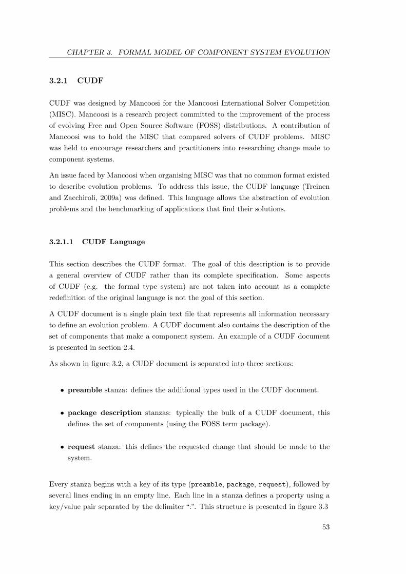
CHAPTER 3. FORMAL MODEL OF COMPONENT SYSTEM EVOLUTION
3.2.1 CUDF
CUDF was designed by Mancoosi for the Mancoosi International Solver Competition
(MISC). Mancoosi is a research project committed to the improvement of the process
of evolving Free and Open Source Software (FOSS) distributions. A contribution of
Mancoosi was to hold the MISC that compared solvers of CUDF problems. MISC
was held to encourage researchers and practitioners into researching change made to
component systems.
An issue faced by Mancoosi when organising MISC was that no common format existed
to describe evolution problems. To address this issue, the CUDF language (Treinen
and Zacchiroli, 2009a) was defined. This language allows the abstraction of evolution
problems and the benchmarking of applications that find their solutions.
3.2.1.1 CUDF Language
This section describes the CUDF format. The goal of this description is to provide
a general overview of CUDF rather than its complete specification. Some aspects
of CUDF (e.g. the formal type system) are not taken into account as a complete
redefinition of the original language is not the goal of this section.
A CUDF document is a single plain text file that represents all information necessary
to define an evolution problem. A CUDF document also contains the description of the
set of components that make a component system. An example of a CUDF document
is presented in section 2.4.
As shown in figure 3.2, a CUDF document is separated into three sections:
• preamble stanza: defines the additional types used in the CUDF document.
• package description stanzas: typically the bulk of a CUDF document, this
defines the set of components (using the FOSS term package).
• request stanza: this defines the requested change that should be made to the
system.
Every stanza begins with a key of its type (preamble, package, request), followed by
several lines ending in an empty line. Each line in a stanza defines a property using a
key/value pair separated by the delimiter “:”. This structure is presented in figure 3.3
53
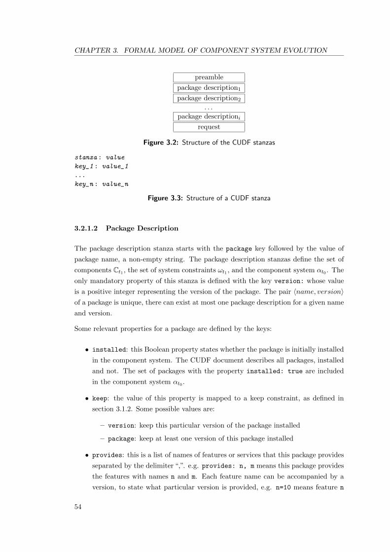
CHAPTER 3. FORMAL MODEL OF COMPONENT SYSTEM EVOLUTION
preamble
package description1
package description2
. . .
package descriptioni
request
Figure 3.2: Structure of the CUDF stanzas
stanza : value
key_1 : value_1
...
key_n : value_n
Figure 3.3: Structure of a CUDF stanza
3.2.1.2 Package Description
The package description stanza starts with the package key followed by the value of
package name, a non-empty string. The package description stanzas define the set of
components Ct1 , the set of system constraints ωt1 , and the component system αt0 . The
only mandatory property of this stanza is defined with the key version: whose value
is a positive integer representing the version of the package. The pair 〈name, version〉of a package is unique, there can exist at most one package description for a given name
and version.
Some relevant properties for a package are defined by the keys:
• installed: this Boolean property states whether the package is initially installed
in the component system. The CUDF document describes all packages, installed
and not. The set of packages with the property installed: true are included
in the component system αt0 .
• keep: the value of this property is mapped to a keep constraint, as defined in
section 3.1.2. Some possible values are:
– version: keep this particular version of the package installed
– package: keep at least one version of this package installed
• provides: this is a list of names of features or services that this package provides
separated by the delimiter “,”. e.g. provides: n, m means this package provides
the features with names n and m. Each feature name can be accompanied by a
version, to state what particular version is provided, e.g. n=10 means feature n
54
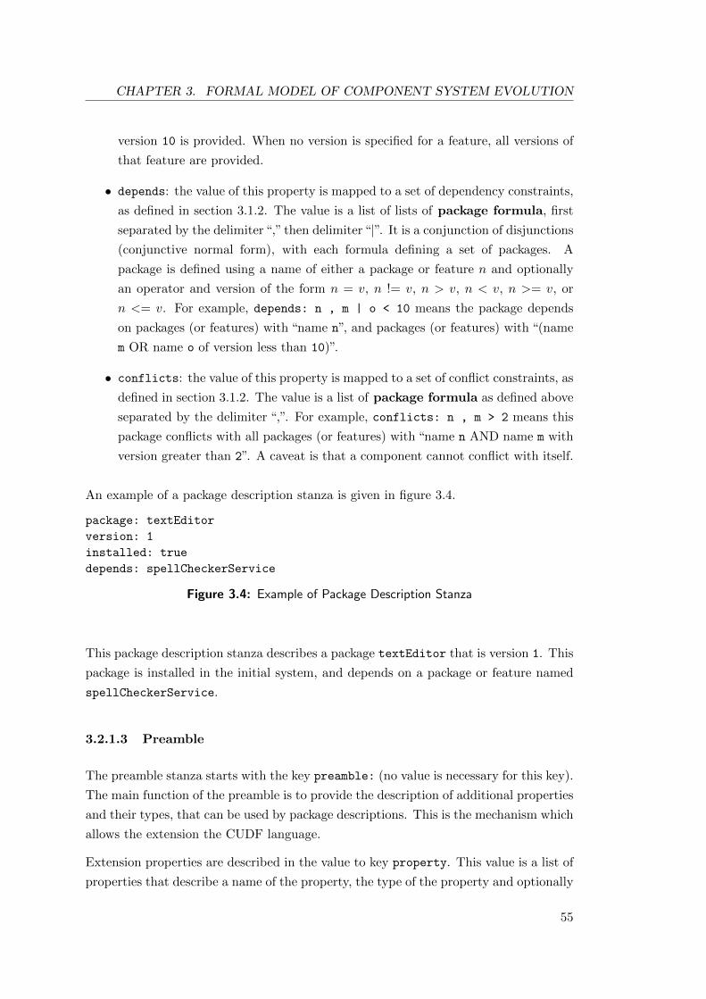
CHAPTER 3. FORMAL MODEL OF COMPONENT SYSTEM EVOLUTION
version 10 is provided. When no version is specified for a feature, all versions of
that feature are provided.
• depends: the value of this property is mapped to a set of dependency constraints,
as defined in section 3.1.2. The value is a list of lists of package formula, first
separated by the delimiter“,” then delimiter“|”. It is a conjunction of disjunctions
(conjunctive normal form), with each formula defining a set of packages. A
package is defined using a name of either a package or feature n and optionally
an operator and version of the form n = v, n != v, n > v, n < v, n >= v, or
n <= v. For example, depends: n , m | o < 10 means the package depends
on packages (or features) with “name n”, and packages (or features) with “(name
m OR name o of version less than 10)”.
• conflicts: the value of this property is mapped to a set of conflict constraints, as
defined in section 3.1.2. The value is a list of package formula as defined above
separated by the delimiter “,”. For example, conflicts: n , m > 2 means this
package conflicts with all packages (or features) with “name n AND name m with
version greater than 2”. A caveat is that a component cannot conflict with itself.
An example of a package description stanza is given in figure 3.4.
package: textEditor
version: 1
installed: true
depends: spellCheckerService
Figure 3.4: Example of Package Description Stanza
This package description stanza describes a package textEditor that is version 1. This
package is installed in the initial system, and depends on a package or feature named
spellCheckerService.
3.2.1.3 Preamble
The preamble stanza starts with the key preamble: (no value is necessary for this key).
The main function of the preamble is to provide the description of additional properties
and their types, that can be used by package descriptions. This is the mechanism which
allows the extension the CUDF language.
Extension properties are described in the value to key property. This value is a list of
properties that describe a name of the property, the type of the property and optionally
55
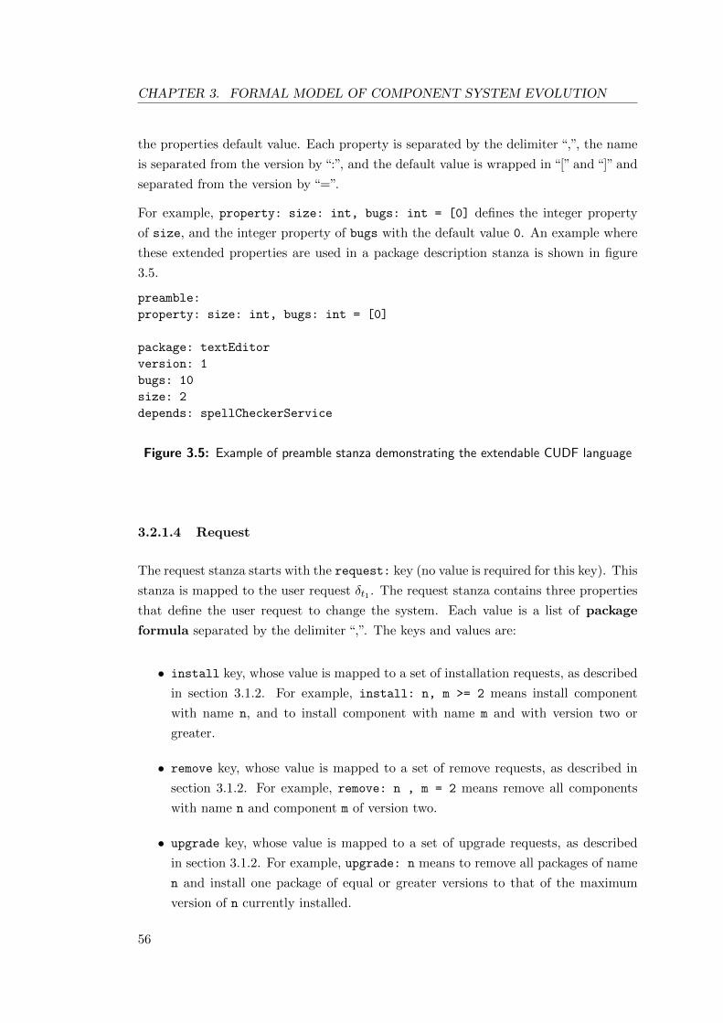
CHAPTER 3. FORMAL MODEL OF COMPONENT SYSTEM EVOLUTION
the properties default value. Each property is separated by the delimiter “,”, the name
is separated from the version by “:”, and the default value is wrapped in “[” and “]” and
separated from the version by “=”.
For example, property: size: int, bugs: int = [0] defines the integer property
of size, and the integer property of bugs with the default value 0. An example where
these extended properties are used in a package description stanza is shown in figure
3.5.
preamble:
property: size: int, bugs: int = [0]
package: textEditor
version: 1
bugs: 10
size: 2
depends: spellCheckerService
Figure 3.5: Example of preamble stanza demonstrating the extendable CUDF language
3.2.1.4 Request
The request stanza starts with the request: key (no value is required for this key). This
stanza is mapped to the user request δt1 . The request stanza contains three properties
that define the user request to change the system. Each value is a list of package
formula separated by the delimiter “,”. The keys and values are:
• install key, whose value is mapped to a set of installation requests, as described
in section 3.1.2. For example, install: n, m >= 2 means install component
with name n, and to install component with name m and with version two or
greater.
• remove key, whose value is mapped to a set of remove requests, as described in
section 3.1.2. For example, remove: n , m = 2 means remove all components
with name n and component m of version two.
• upgrade key, whose value is mapped to a set of upgrade requests, as described
in section 3.1.2. For example, upgrade: n means to remove all packages of name
n and install one package of equal or greater versions to that of the maximum
version of n currently installed.
56
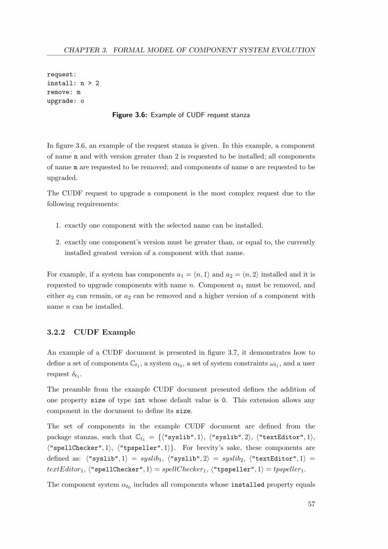
CHAPTER 3. FORMAL MODEL OF COMPONENT SYSTEM EVOLUTION
request:
install: n > 2
remove: m
upgrade: o
Figure 3.6: Example of CUDF request stanza
In figure 3.6, an example of the request stanza is given. In this example, a component
of name n and with version greater than 2 is requested to be installed; all components
of name m are requested to be removed; and components of name o are requested to be
upgraded.
The CUDF request to upgrade a component is the most complex request due to the
following requirements:
1. exactly one component with the selected name can be installed.
2. exactly one component’s version must be greater than, or equal to, the currently
installed greatest version of a component with that name.
For example, if a system has components a1 = 〈n, 1〉 and a2 = 〈n, 2〉 installed and it is
requested to upgrade components with name n. Component a1 must be removed, and
either a2 can remain, or a2 can be removed and a higher version of a component with
name n can be installed.
3.2.2 CUDF Example
An example of a CUDF document is presented in figure 3.7, it demonstrates how to
define a set of components Ct1 , a system αt0 , a set of system constraints ωt1 , and a user
request δt1 .
The preamble from the example CUDF document presented defines the addition of
one property size of type int whose default value is 0. This extension allows any
component in the document to define its size.
The set of components in the example CUDF document are defined from the
package stanzas, such that Ct1 = 〈"syslib", 1〉, 〈"syslib", 2〉, 〈"textEditor", 1〉,〈"spellChecker", 1〉, 〈"tpspeller", 1〉. For brevity’s sake, these components are
defined as: 〈"syslib", 1〉 = syslib1, 〈"syslib", 2〉 = syslib2, 〈"textEditor", 1〉 =
textEditor1, 〈"spellChecker", 1〉 = spellChecker1, 〈"tpspeller", 1〉 = tpspeller1.
The component system αt0 includes all components whose installed property equals
57

CHAPTER 3. FORMAL MODEL OF COMPONENT SYSTEM EVOLUTION
preamble:
property: size: int = [0]
package: syslib
version: 1
installed: true
package: syslib
version: 2
conflicts: syslib
package: textEditor
version: 1
depends: spellChecker | spellCheckerService, syslib > 1
package spellChecker
version: 1
size: 1
package: tpspeller
version: 1
provides: spellCheckerService
size: 2
request:
install:textEditor
Figure 3.7: Example of a CUDF document
true (it defaults to false), αt0 = syslib1.
The system constraints ωt1 can be extracted from the example CUDF document. These
are defined by the depends property of textEditor1, and the conflicts property of
syslib2.
textEditor1 depends on spellChecker or spellCheckerService AND syslib
greater than version 1. The first dependency is on components that are named
spellChecker or spellCheckerService, or provide a feature named spellChecker or
spellCheckerService. Components that satisfy this criteria are spellChecker1 and
tpspeller1. This results in the dependency constraint textEditor1 → spellChecker1 ∨tpspeller1.
The second dependency is on components that are named syslib greater than
version 1, or provide a feature named syslib with version greater than 1. The
only component that satisfies this dependency is syslib2, resulting in the dependency
58
CHAPTER 3. FORMAL MODEL OF COMPONENT SYSTEM EVOLUTION
constraint textEditor1 → syslib2.
syslib2 conflicts with components of name syslib, that is not itself. The only
component that satisfies this conflict is syslib1, resulting in the conflict constraint
syslib2 → ¬syslib1.
The set of system constraints ωt1 in the example CUDF document is textEditor1 →spellChecker1 ∨ tpspeller1, textEditor1 → syslib2, syslib2 → ¬syslib1.
The user request δt1 is defined by the example CUDF documents request stanza.
The request is to install a package named textEditor. The only component that
satisfies this description is textEditor1, which results in the install request textEditor1.
Therefore, δt1 = textEditor1.
The evolution problem δt1 ∪ ωt1 can be found by looking at the constraints defined
by each package description and the request. Firstly, the request constraints ensures
that textEditor1 must be installed. If textEditor1 is installed then the system library
component syslib2 must be installed, given textEditor1 → syslib2. As syslib2 conflicts
with syslib1, syslib1 must not be installed. spellChecker1 or tpspeller1 must be
installed, given textEditor1 → spellChecker1 ∨ tpspeller1.
The three possible solutions to this evolution problem are;
• α1t1 = syslib2, textEditor1, spellChecker1,
• α2t1 = syslib2, textEditor1, tpspeller1,
• α3t1 = syslib2, textEditor1, spellChecker1, tpspeller1
3.2.3 Mancoosi Optimisation Format
MOF is a format defined by Mancoosi to express the lexicographic order of criteria.
The definition of what the criteria are is external to MOF. A criterion is directly defined
in CoSyE and MOF is only used to define the lexicographic order.
A MOF string is a list of lexicographically ordered criterion names separated by
the delimiter “,”. Each criterion name is mapped to a criterion in CoSyE. A MOF
string is therefore mapped to an evolution preference order by using the lexicographic
composition of criteria defined in the string.
An example is presented to show how a MOF string can be used to create an evolution
preference order. This preference order is then applied to the example presented in
section 3.2.2 to find the optimal solution.
59
CHAPTER 3. FORMAL MODEL OF COMPONENT SYSTEM EVOLUTION
A criterion is defined to minimise the change to a component system during evolution.
This criterion’s name is -changed in MOF, and is defined as critchange = 〈rankchangeαt0,≤
〉, where rankchangeαt0(β) = |αt0∆β|.
Another criterion is defined to minimise the total size of the component system. This
criterion’s name is -size in MOF, and is defined as critsize = 〈ranksizeαt0,≤〉, where
ranksizeαt0(β) =
∑c∈β c.size.
The MOF string -change,-size defines the lexicographically composed criteria
critchange⊕critsize which equals 〈rankLαt0,≤L〉 (as shown in definition 18). This criterion
can be used to create an evolution preference order ≺αt0(as described in definition 17).
In the previous example, the component system αt0 was syslib1, and there were three
possible solutions:
• α1t1 = syslib2, textEditor1, spellChecker1,
• α2t1 = syslib2, textEditor1, tpspeller1,
• α3t1 = syslib2, textEditor1, spellChecker1, tpspeller1
This rank function rankLαt0applied to the possible solutions returns pairs of (rankchangeαt0
,
ranksizeαt0):
• rankLαt0(α1
t1) = r1 = (4, 1), i.e. change is 4 and size is 1.
• rankLαt0(α2
t1) = r2 = (4, 2), i.e. change is 4 and size is 2.
• rankLαt0(α3
t1) = r3 = (5, 3), i.e. change is 5 and size is 3.
The order of these ranks over ≤L is then r3 ≤L r2 ≤L r1. The order of optimality
(≺αt0) over the possible solutions is α3
t1 ≺αt0α2t1 , α3
t1 ≺αt0α1t1 , and α2
t1 ≺αt0α1t1 . This
makes α1t1 an optimal solution, as no other solutions is greater w.r.t. ≺αt0
. Therefore,
given the CUDF document in figure 3.7 and MOF criteria -change,-size the resolved
system is syslib2, textEditor1, spellChecker1.
3.2.4 CUDF*
CUDF* is an extension of both CUDF and MOF, created to define a single document
that can be mapped to an instance of CoSyE. The differences between CUDF and
CUDF* are:
60

CHAPTER 3. FORMAL MODEL OF COMPONENT SYSTEM EVOLUTION
• In CUDF* each package description stanza must define the time that the
component first existed.
• In CUDF* the preamble defines the time t0.
• In CUDF* there can be multiple requests stanza’s, where each request stanza
must define a time ti, and MOF criteria string such that the request stanza maps
to the request δti to ≺αti−1.
• In CUDF* an upgrade request with value * attempts to upgrade all installed
components.
By defining when each package first existed, the set of components Cti can be found for
any arbitrary time ti. Additionally, the system constraints ωti can also be extracted.
The overall structure of a CUDF* document where the preamble defines t0, and there
are multiple requests each defining a time is presented in figure 3.8.
preamblet0package description1
package description2
. . .
package descriptioni
requestt1requestt2
. . .
requesttj
Figure 3.8: Structure of the CUDF* stanzas
With these extensions, a CUDF* document is able to define the necessary elements in
an instance of CoSyE. A full description of the process of parsing a CUDF* document
to a CoSyE instance can be found in appendix A.
3.2.5 CUDF* Example
An example of a CUDF* document is presented in figure 3.9 that is similar to the
example presented in 3.7. This example is designed to demonstrate the differences
between CUDF, MOF and CUDF*.
Parsing this CUDF* document results in:
• The initial component system αt0 which is the set syslib1 (the same from the
previous example).
61
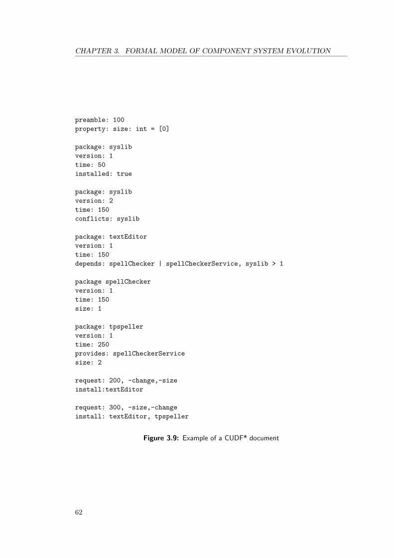
CHAPTER 3. FORMAL MODEL OF COMPONENT SYSTEM EVOLUTION
preamble: 100
property: size: int = [0]
package: syslib
version: 1
time: 50
installed: true
package: syslib
version: 2
time: 150
conflicts: syslib
package: textEditor
version: 1
time: 150
depends: spellChecker | spellCheckerService, syslib > 1
package spellChecker
version: 1
time: 150
size: 1
package: tpspeller
version: 1
time: 250
provides: spellCheckerService
size: 2
request: 200, -change,-size
install:textEditor
request: 300, -size,-change
install: textEditor, tpspeller
Figure 3.9: Example of a CUDF* document
62
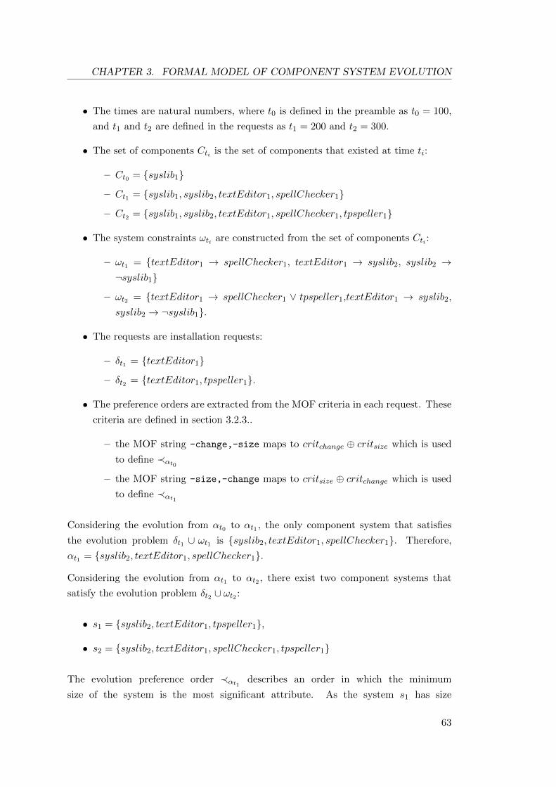
CHAPTER 3. FORMAL MODEL OF COMPONENT SYSTEM EVOLUTION
• The times are natural numbers, where t0 is defined in the preamble as t0 = 100,
and t1 and t2 are defined in the requests as t1 = 200 and t2 = 300.
• The set of components Cti is the set of components that existed at time ti:
– Ct0 = syslib1
– Ct1 = syslib1, syslib2, textEditor1, spellChecker1
– Ct2 = syslib1, syslib2, textEditor1, spellChecker1, tpspeller1
• The system constraints ωti are constructed from the set of components Cti :
– ωt1 = textEditor1 → spellChecker1, textEditor1 → syslib2, syslib2 →¬syslib1
– ωt2 = textEditor1 → spellChecker1 ∨ tpspeller1,textEditor1 → syslib2,
syslib2 → ¬syslib1.
• The requests are installation requests:
– δt1 = textEditor1
– δt2 = textEditor1, tpspeller1.
• The preference orders are extracted from the MOF criteria in each request. These
criteria are defined in section 3.2.3..
– the MOF string -change,-size maps to critchange ⊕ critsize which is used
to define ≺αt0
– the MOF string -size,-change maps to critsize ⊕ critchange which is used
to define ≺αt1
Considering the evolution from αt0 to αt1 , the only component system that satisfies
the evolution problem δt1 ∪ ωt1 is syslib2, textEditor1, spellChecker1. Therefore,
αt1 = syslib2, textEditor1, spellChecker1.
Considering the evolution from αt1 to αt2 , there exist two component systems that
satisfy the evolution problem δt2 ∪ ωt2 :
• s1 = syslib2, textEditor1, tpspeller1,
• s2 = syslib2, textEditor1, spellChecker1, tpspeller1
The evolution preference order ≺αt1describes an order in which the minimum
size of the system is the most significant attribute. As the system s1 has size
63

CHAPTER 3. FORMAL MODEL OF COMPONENT SYSTEM EVOLUTION
2, and the system s2 has size 3, the optimal solution is s1. Therefore, αt2 =
syslib2, textEditor1, tpspeller1.
This CUDF* document therefore describes the evolution of a component system from
syslib1, to syslib2, textEditor1, spellChecker1, then to syslib2, textEditor1, tpspeller1.
This example demonstrates how a CUDF* document can be used to describe the
evolution of a component system.
3.3 Summary
This chapter described the CoSyE model and the CUDF* language. These are used to
describe the evolution of a component systems as a series of change requests made to
the system by a user. These changes are subject to constraints that must be satisfied in
order to result in a valid system. These describe the evolution of a system and not the
user that requests changes to the system. The following chapter defines the SimUser
model that describes the user, their system, and the changes they make.
64

Chapter 4
User Model
All parts should go together without forcing. You must remember that the parts
you are reassembling were disassembled by you. Therefore, if you can’t get them
together again, there must be a reason. By all means, do not use a hammer.
IBM maintenance manual, 1925
In the previous chapter, CUDF* documents were used to describe the evolution of
component systems through a user’s repeated requests to change. Given that a goal of
this research is to simulate the evolution of component systems, it is necessary to model
realistic users. For this purpose the SimUser (Simulated User) model was developed.
This model describes how a user would change systems, and it can be used to create
CUDF* documents. These relationships are described in figure 4.1.
CUDF*
:CUDF* Document
ins tan t ia tes
:SimUser c rea tes
SimUser
ins tan t ia tes
Figure 4.1: Relationships between the SimUser model and CUDF*
The SimUser model was developed using the results of a survey conducted to determine
how users change their component systems. This survey is described in section 4.1.
SimUser contains variables to create a realistic scenario of CSE, e.g. a variable that
describes the probability a user will upgrade their system on a given day. In addition
it contains assumptions (e.g. the probability a package will be selected to be installed)
made in the simulation. SimUser is presented in section 4.2 and the variables and
assumptions for the simulation are discussed.
65
CHAPTER 4. USER MODEL
In order to define parts of SimUser it was necessary to collect and convert data into
usable formats. The sources this data was collected from and the methods used to
convert it are described in section 4.3.
This chapter concludes in section 4.4 with a discussion over the validity of SimUser,
focusing on the differences from the reality of CSE. These differences are important to
explore, as they may reduce the validity of the results from the simulation.
4.1 User Survey
To explore the user’s role in CSE and to construct the SimUser model, a survey was
conducted on users of component systems. This survey targeted users of GNU/Linux
distributions (specifically Ubuntu) and server administrators through the online forum
reddit1. It was completed by 59 users, who answered questions about their background,
the systems they use, and the ways they change their systems. Typically the way in
which GNU/Linux systems are changed is through interaction with package manager
applications. Therefore, the questions were primarily about this interaction.
In this section, a description of the survey and an analysis of responses are given.
The results from this survey are used to describe and categorise the motivations and
behaviours of users when changing their component systems.
4.1.1 Questions
The survey consisted of two groups of questions: questions that identified the type of
user and questions that described their interactions with package managers. These were
asked in order to understand the user and how and why they changed their systems.
The set of questions used to identify the user were:
• How experienced with package managers are you (based on scale of 1 to 5 where
1 is no experience and 5 is highly experienced)?
• What system are you using?
• What package manager are you using?
These can be used to categorise the type of user and weigh their answers for credibility
based on their self rated experience.
The set of questions that asked about the use of package managers were:
1http://reddit.com accessed 6/3/2012
66
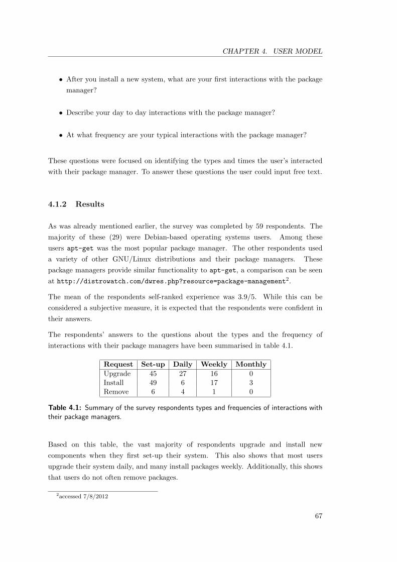
CHAPTER 4. USER MODEL
• After you install a new system, what are your first interactions with the package
manager?
• Describe your day to day interactions with the package manager?
• At what frequency are your typical interactions with the package manager?
These questions were focused on identifying the types and times the user’s interacted
with their package manager. To answer these questions the user could input free text.
4.1.2 Results
As was already mentioned earlier, the survey was completed by 59 respondents. The
majority of these (29) were Debian-based operating systems users. Among these
users apt-get was the most popular package manager. The other respondents used
a variety of other GNU/Linux distributions and their package managers. These
package managers provide similar functionality to apt-get, a comparison can be seen
at http://distrowatch.com/dwres.php?resource=package-management2.
The mean of the respondents self-ranked experience was 3.9/5. While this can be
considered a subjective measure, it is expected that the respondents were confident in
their answers.
The respondents’ answers to the questions about the types and the frequency of
interactions with their package managers have been summarised in table 4.1.
Request Set-up Daily Weekly Monthly
Upgrade 45 27 16 0Install 49 6 17 3Remove 6 4 1 0
Table 4.1: Summary of the survey respondents types and frequencies of interactions withtheir package managers.
Based on this table, the vast majority of respondents upgrade and install new
components when they first set-up their system. This also shows that most users
upgrade their system daily, and many install packages weekly. Additionally, this shows
that users do not often remove packages.
2accessed 7/8/2012
67
CHAPTER 4. USER MODEL
4.1.3 Progressive vs. Conservative Users
One goal of this survey was to identify motivations of users’ to change their systems.
Based on the responses the users attitudes towards changing their systems are affected
by the following risks:
• the potential risk of changing the system and introducing new problems.
• the potential risk of becoming out-of-date, having less functionality, and having
old problems persist.
The behaviours of these users can be described with two user stereotypes, conservative
and progressive. These terms come from the domain of politics where conservatism
philosophy that emphasises minimal and gradual change in society, which is contrasted
by progressivism philosophy that promotes change and reform (Online Oxford English
Dictionary, 2010).
Most users in the survey are partially motivated by both risks, e.g. a user’s response
that expresses a slight conservative attitude:
“In production I rarely remove packages ([it is] easier to leave software
as-is than risk breaking stuff).”
This quote shows that this respondent is less likely to change their system, even though
it may be beneficial.
Another example of a user’s response that expresses a progressive attitude:
“I update my packages whenever I log in each day”
The reason this user upgrades their system every day is likely to ensure that packages do
not become out-of-date. This behaviour may increase the functionality of their system
and allow bugs in packages to be fixed, though it has the cost of additional change.
Both of these stereotypes have extremes. One such extreme is when a user tries
to eliminate all of the risks associated with being out-of-date. For example, a user
responded in the survey with an extreme progressive attitude:
“I do run an unstable system all the time, I help mitigate this with some
redundancy in my most frequently used components, using packages which
perform the same function, but have different dependencies, since it’s less
68
CHAPTER 4. USER MODEL
likely to have multiple packages break at the same time. If something is
rather buggy for me, I tend to update on a more frequent basis to check for
the next stable point to jump into.”
This user has components in their system that have not been thoroughly tested
(described as unstable packages). To lower the risk that such packages have on the
function of the system, this user has redundant functionality installed. This way the
user tries to ensure that potential problems will not be too severe. The system of this
user will never be out-of-date, but will be changed frequently.
An example of a very conservative user’s response on the frequency with which they
interact with the package manager:
“As little as possible. I like build my box into whatever I’ll need in
the first couple of weeks after an install. Following the configuration and
construction, only the occasional upgrade is necessary. Unless, of course, I
receive a security notice about something.”
After the setting up of a system, this user will not change it unless there is a direct
security risk. This lack of change will result in the system quickly becoming out-of-date.
The “progressive” and “conservative” terminology is useful to describe different types of
users and their motivations. It is used further when describing the simulated users in
chapter 6.
4.2 SimUser model
The SimUser model consists of:
• a set of variables that describe the user’s behaviour when changing their
component system.
• a set of assumptions used by the simulation.
This section presents the variables and assumptions of SimUser, and how an instance
of this model can be used to create a CUDF* document.
4.2.1 Variables and Assumptions
The SimUser entity consists of the following variables:
69
CHAPTER 4. USER MODEL
• u is the probability a user requests to upgrade the system per day.
• i is the probability a user requests to install any component per day.
• U is the MOF criteria used to select an optimal system for an upgrade request.
• I is the MOF criteria used to select an optimal system for an install request.
An instance of SimUser is an assignment to these variables.
The variable u is the probability per day that a user will upgrade their system, and the
variable i is the probability a user will request to install a component. The reason for
selecting the “per day” resolution came from the user survey responses where typically
the most frequent a user interacted with a package manager was daily. The I and U
criteria to install a component and upgrade a system are represented in MOF. These
criteria can be based on package manager criteria from currently installed applications
like apt-get or on novel criteria.
The assumptions made in the SimUser model are:
• The starting time of the evolution t0 is October 30th 2009.
• The initial component system αt0 is Ubuntu 9.10 (i386) released October 29th
2009.
• The user interacts with the system over a year (365 days).
• The available components to the evolving system are located at the central
Ubuntu repository.
• Each component name has a probability that a user will select to install it.
The reason for selecting Ubuntu as the system to simulate is discussed in chapter 1.
The time frame, October 2009 to 2010, was selected to start at the release of Ubuntu
9.10 until the release of Ubuntu 10.10. A year was selected as 30/59 respondents of the
survey stated that their systems are less than or about one year old. The Ubuntu system
has 6 monthly releases, therefore the simulation will be over the release of Ubuntu 10.04
in April 2010.
The Ubuntu central repository is the core location for where packages are distributed
to Ubuntu systems. Using this as the set of packages because it is the default choice of
newly installed Ubuntu systems.
Typically a user would not select a specific version of a package to be installed but
select the package name and let the package manager install the most preferred version
70
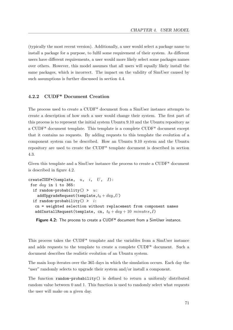
CHAPTER 4. USER MODEL
(typically the most recent version). Additionally, a user would select a package name to
install a package for a purpose, to fulfil some requirement of their system. As different
users have different requirements, a user would more likely select some packages names
over others. However, this model assumes that all users will equally likely install the
same packages, which is incorrect. The impact on the validity of SimUser caused by
such assumptions is further discussed in section 4.4.
4.2.2 CUDF* Document Creation
The process used to create a CUDF* document from a SimUser instance attempts to
create a description of how such a user would change their system. The first part of
this process is to represent the initial system Ubuntu 9.10 and the Ubuntu repository as
a CUDF* document template. This template is a complete CUDF* document except
that it contains no requests. By adding requests to this template the evolution of a
component system can be described. How an Ubuntu 9.10 system and the Ubuntu
repository are used to create the CUDF* template document is described in section
4.3.
Given this template and a SimUser instance the process to create a CUDF* document
is described in figure 4.2.
createCUDF*(template, u, i, U, I):for day in 1 to 365:
if random-probability() > u:addUpgradeRequest(template,t0 + day,U)
if random-probability() > i:cn = weighted selection without replacement from component names
addInstallRequest(template, cn, t0 + day + 10 minutes,I)
Figure 4.2: The process to create a CUDF* document from a SimUser instance.
This process takes the CUDF* template and the variables from a SimUser instance
and adds requests to the template to create a complete CUDF* document. Such a
document describes the realistic evolution of an Ubuntu system.
The main loop iterates over the 365 days in which the simulation occurs. Each day the
“user” randomly selects to upgrade their system and/or install a component.
The function random-probability() is defined to return a uniformly distributed
random value between 0 and 1. This function is used to randomly select what requests
the user will make on a given day.
71
CHAPTER 4. USER MODEL
If a user requests to upgrade their system, the function addUpgradeRequest adds an
upgrade request to the CUDF template at time initial time t0 plus the number of
elapsed days. This request uses the MOF criteria U to find an optimal system. If the
user requests to install a component, a component to be installed must first be selected.
This selection is:
• Weighted : names with a higher weight are more likely to be requested to be
installed.
• Without replacement : a user cannot select to install the same component name
more than once.
The function addInstallRequest adds an install request to the CUDF template ten
minutes after the initial time t0 plus the number of elapsed days. Adding ten minutes
ensures that if a user selects to upgrade and install a component, then the installation
request will occur after the upgrade request. The install request will use the criteria I
from the user model.
The discussion over the validity of the resulting CUDF* documents is presented in
section 4.4.
4.3 SimUser Data Collection and Conversion
In order to create CUDF* documents from SimUser instances, data about the Ubuntu
system must be collected and converted into useful formats. The collected data and
their sources are:
1. The set of Ubuntu packages and the times they became available, collected from
the Ubuntu repository.
2. The initial component system Ubuntu 9.10 collected from a virtual install.
3. The probabilities different component names will be selected to be installed,
from the app-install-data package and weighted using the Ubuntu popularity
contest3.
This section describes the data collection and conversion to create SimUser.
3http://popcon.ubuntu.com/ accessed 6/3/2012
72
CHAPTER 4. USER MODEL
4.3.1 Collecting the Components
The Ubuntu repository located at http://archive.ubuntu.com/ is the default location
that Ubuntu packages are distributed from. This repository contains a history of all
packages that have ever been included with the precise minute that the package was
uploaded.
To collect these packages and information from the repository first the repository’s web
site was parsed and all the packages were downloaded. These Debian/Ubuntu packages
are compressed with meta-information, code and binary files.
Second, each package was decompressed and the main meta-data file, the control file,
was extracted. This control file was tagged with the upload time of the package to the
Ubuntu Repository.
Third, all control files that did not have the key architecture include the value i386
or all where removed. This removes any package that would not work on the simulated
Ubuntu system due to architecture incompatibility.
Fourth, the control files are converted into a single CUDF* document. The conversion
from Debian control files to a CUDF document is described by Abate et al. (2010).
This report describes the handling of virtual packages and the conversion of versions.
This process is followed to create the CUDF* template with the exceptions that:
• apt-pinning priorities that force the use of only particular versions of a package
are ignored.
• If a package has the value require for key priority, the CUDF* package is given
the property keep: package to ensure the package remains between requests.
• In the preamble the time t0 is added.
• Each CUDF package has the key time added with the tagged time of their control
file.
• A self conflict is not added to each package to simulate the restraint that only
one version of each package is allowed to be installed.
The final difference is significant as it differs from how real Ubuntu systems evolve and
could invalidate the simulations results. However, the restriction for these systems to
only allow one version to be installed is an interesting point of study. By allowing
multiple packages to be installed means that this specific constraint can be studied.
For example, questions like “how often does an install request require the installation
73
CHAPTER 4. USER MODEL
of multiple packages?” or “how much does does this restriction effect the evolution of
Ubuntu systems?” can be answered by not enforcing this restriction. It is still preferable
for a user to not have multiple versions of a package. Therefore, this restriction can
be “softly” enforced through using a criterion to minimise the number of packages with
multiple versions. Such a criterion is defined in section 5.2.3 and it is shown in chapter
6 that this alteration has almost no impact on the simulation.
4.3.2 Probability a component will be selected
Different users will likely select different components to install. For example, a user who
is a graphic designer will more likely select graphics editor tools to be installed, and less
likely select programming tools. To simulate each user with their individual preferences
of what they would install is impractical. For this simulation each component name’s
probability to be installed will be the same for all users.
To define the probability a user will select a component to install, the problem is broken
into two questions:
1. What component would a user select to install?
2. How often are these components selected to be installed?
There are many packages in the Ubuntu repository that a user would not likely select
for install. Packages that provide libraries, background daemons, interfaces between
services are usually installed because other packages depend on them, not because a
user selected to install them. What packages would a user select to install and how
likely they will be selected are therefore important questions. By looking at current
systems and what packages they have installed, the probability that these packages are
selected to be installed can be estimated. These questions are answered using data
from the package app-install-package and the Ubuntu popularity contest.
The package app-install-package contains a list of 2399 packages4 with meta-data
like icons and descriptions. This data is used by other applications, like the Ubuntu
Software Center, to provide a list of packages the user may wish to install. Some of
these packages are installed by default in Ubuntu systems, and some are not available
in the Ubuntu repository. After filtering out such packages from the provided list there
remain 2087 packages that the user may select to install in their system.
The probability a package from the app-install-package list is selected to be installed
can be calculated using the Ubuntu popularity contest. The Ubuntu popularity contest
4as of May 24th 2011
74

CHAPTER 4. USER MODEL
is a broad data-set of information of the popularity of Ubuntu packages. Each week an
automated survey is submitted by nearly two million users, that contains information
on what packages a user has installed. The results from this survey are processed
and the number of systems that have a package installed is presented in the Ubuntu
popularity contest. By dividing the the number of systems each package from the app-
install-data packages by the total survey respondents, the probability a package is
selected to be installed is estimated.
4.4 SimUser Validation
The validation of SimUser has been accomplished through:
• Discussions with project supervisors and other stakeholders.
• Comparing SimUser to the responses from the user survey.
• Compare generated CUDF* documents with apt-get logs collected from 19
respondents of the survey5.
• Creating a virtual Ubuntu 11.10 system to study its perspective of the Ubuntu
repository changing over the month of November 2011.
Using these methods differences between the simulation and the reality of CSE can
be identified and discussed. These differences largely come from the randomness in
SimUser, e.g. randomly selecting packages to install, and from the limitations of the
model, e.g. the limited types of request. Additional differences exist in the way in
which SimUser uses the Ubuntu repository. This section discusses these differences and
their impacts on the validity of SimUser.
4.4.1 Randomness of SimUser
When generating a CUDF* document, each simulated day there are three points of
randomness in SimUser:
1. The probability a user requests to upgrade their system, u.
2. The probability a user requests to install a component, i.
3. If the user requests to install, what package is selected to be installed.
5Comparing these logs to the resulting simulated systems is described in section 5.5
75
CHAPTER 4. USER MODEL
In reality, a user’s request to upgrade the system or install a component are not random.
These requests are reasoned about using gathered information, preferences and external
constraints. Even the most insignificant aspect of a user may impact requests, e.g. the
favourite colour of a user may impact their choices of components to install. To model
a user completely would be difficult, if not impossible, and would require significant
effort. SimUser instead simulates the user with random behaviour. The impact on
validity of the randomness of these behaviours is discussed here.
The variables u and i introduce randomness into the simulation that does not exist in
the evolution of real component systems. For example, a user who upgrades their system
each work day (Monday to Friday) would have a probability to upgrade their system
as 5/7. Describing such a user with SimUser and then generating a CUDF* document
may create a situation where they will upgrade their system on a Saturday. This is
because users will not randomly select days to request changes, they have constraints
(like the work week) and preferences that are not expressed in this model.
The most significant randomness in SimUser comes from the selection of components
to be installed. This randomness causes many differences to the reality of CSE:
• A real user would typically not randomly select a component to be installed. A
user would likely research a component before deciding to install.
• Each user would have different preferences of which components to install, e.g. a
software developer will prefer components to aid in software development.
• Installing one package may change the preference of installing another, e.g.
installing of browser firefox would decrease the probability to install another
browser such as chromium.
To address these issues would require a more data to be collected and the modifications
would make SimUser significantly more complex. The reduced effort and cost during
data collection and the simplicity of the model was decided to take priority in this
matter.
To mitigate the randomness in SimUser many CUDF* documents will be created from
a single SimUser instance, then simulated. The results from these simulations can then
be aggregated and analysed. Additionally, any conclusions derived from the results will
be tempered by being aware of the randomness in SimUser.
An important caveat to note is that there exist two assignments to the variables u and
i that result in users that are not at all random:
1. Control user: u = 0 and i = 0
76
CHAPTER 4. USER MODEL
2. Always Upgrade user: u = 1 and i = 0
The “Control” user never requests to change their system, therefore their system will
always be the initial system and never evolve. The “Always Upgrade” user will update
every day, and given two users that have the same upgrade criteria U , their systems
will evolve identically. These effects of these two users are further discussed in chapter
6.
4.4.2 Limitations of SimUser
The limitations that SimUser has are:
• The initial set-up of the system by the user (as described in the user survey) is
not included.
• Some types of requests are not included, notably remove requests.
• Cannot request to install many components on the same day, or at the same time.
• The list of packages that can be installed (from app-install-data) does not
include many commonly installed packages.
Each of these points will be addressed in order.
The initial set-up of a system, which is performed by many respondents of the user
survey, is not included in SimUser. This set-up includes upgrading their system,
installing and removing components. The initial upgrade is superfluous in the
simulation as the initial system is already uptodate. The initial installation and removal
of components is not simulated as it will create different starting systems for different
users, making comparison between users more difficult.
In a real Ubuntu system, a user may request many different types of action, e.g. the
remove component request. Respondents to the user survey stated they request to
remove a component infrequently, this is supported by the data in the user logs. This
is the justification for the exclusion from the SimUser.
A user may want to install many components during a single day. This can be
accomplished with one request to install many components or many requests to
install single components. Both these situations commonly occur in the submitted
user logs. For example, apt-get install ia32-libs ia32-libs-gtk libqt4-core
libqt4-gui is a single request to install multiple components, and apt-get install
autoconf and apt-get install checkinstall are two requests performed on the
77
CHAPTER 4. USER MODEL
same day. Given the significant randomness in selecting a component to be installed,
introducing either of these situations into SimUser would only make results less valid.
For this reason, a user requesting to install many components on a single day is not
simulated.
In reality, a user often requests to install packages that are not included in the list
from the app-install-data package. An example of this extracted from the user logs
is apt-get install build-essential6, this package cannot be installed during the
simulation as it is not in the list from app-install-data. Much effort that went into
creating SimUser was directed at finding a list of the most commonly installed packages.
However, the core problem is that there exists very little information on what packages
users commonly request to be installed. This problem is seen as a possible future
research that is described in chapter 7.
4.4.3 Perspective of the Ubuntu Repository
In a real Ubuntu system only a subset of the packages in the Ubuntu repository is
visible to the package manager. This “view” of the repository is the set of packages
considered when resolving a request. This is different to CoSyE and SimUser, where
every request can consider all components that exist at the time of the request.
To study the difference this view of the repository has to the simulation a virtual Ubuntu
11.10 system was created, and each day in the month of November 2011 the subset of
components in its view of Ubuntu repository was stored. This system used only the
default “view” of the Ubuntu repository. This “view” is compared to the changes in the
repository of components over the month November 2009 in the SimUser repository.
The SimUser repository contains about 90,000 different package names, where the
virtual “view” contained only about 40,000. This difference is made up mostly of
deprecated packages, i.e. packages that are no longer actively maintained. It is also
made up of packages that are have not yet been validated and put into the main “view”,
e.g. experimental packages. This causes the mean amount of packages that have a new
version added to the repository to be much higher in the SimUser repository, 126
packages per day compared to the virtual systems view of 37 packages per day.
The most significant difference though is the amount of removed packages from the
“view”. The mean amount of packages removed per day from the view of the Ubuntu
repository is eight, where the SimUser repository never removes a package. This removal
of packages reduces the complexity of the problem, though it also means that a real
6build-essential contains tools to build Debian packages
78
CHAPTER 4. USER MODEL
Ubuntu system may not have all information available when satisfying user requests.
The reason a “view” of the repository was not used in the simulation is due to the fact
that no data-source could be found that saved the set of packages that could be viewed
in the Ubuntu repository at a particular time. This lack of data lead to the decision
that all components should be used.
4.5 Summary
This chapter presented the SimUser model which is used to describe how a realistic
user requests changes to their system. This model was partially created from a survey,
whose results were presented and discussed. The variables that make up the SimUser
and the process used to create CUDF* documents were then described. The data that
was used to create the SimUser was then described with the processes to collect and
convert it. The validation of SimUser was then described, and the differences to the
reality of CSE discussed. By exploring the differences to the reality of CSE the results
from a simulation can be more accurately interpreted.
Although the SimUser model can be used to create a description of the evolution of
a component system, it may require significant calculation to find how exactly the
component system evolves. The constraints of each request must be satisfied, and the
optimal system w.r.t. the criteria must be found. The following chapter presents the
mapping of an instance of CoSyE to a series of problems and the algorithms to solve
such problems. These algorithms are implemented in GJSolver, which is the final piece
required to simulate CSE.
79

CHAPTER 4. USER MODEL
80
Chapter 5
Resolving CoSyE Instances
What I cannot create, I do not understand.
Richard Feynman, 1988
The CoSyE model, presented in chapter 3, describes the evolution of a component
system as a series of evolution steps. In this model, each evolution step alters the
component system to satisfy a user’s request to change it. Calculation of all the systems
that occur as a result of these requests is described as resolving a CoSyE instance.
Resolving a CoSyE instance can require significant computational effort due to the
complexity of finding a satisfactory system for each request. Therefore efficient problem
representations and algorithms are required. One way to resolve a CoSyE instance is to
map each evolution step to a Boolean Lexicographic Optimization (BLO) problem (Joao
et al., 2011). BLO problems consist of finding an assignment to Boolean variables that
satisfies a set of constraints and is optimal with respect to lexicographically ordered
criteria. The constraints can be clauses and linear inequalities defined using a SAT
formula extended with pseudo-Boolean (PB) constraints (SAT+PB) (Dixon, 2004).
Each criterion is defined to either maximise or minimise a PB function. Section 5.1
describes the BLO problem and its mapping to an evolution step from a CoSyE instance.
These relationships are presented in figure 5.1.
The algorithm employed to solve BLO problems is the lexicographic-iterative-
strengthening (LIS) algorithm. This algorithm uses the Davis-Putnam-Logemann-
Loveland (DPLL) (Davis and Putnam, 1960; Davis et al., 1962) algorithm to find
solutions to SAT+PB problems and the iterative strengthening (Calistri-Yeh, 1994; Le
Berre and Parrain, 2010) algorithm to optimise finding a solution. The LIS algorithm
is similar to the “iterative pseudo-Boolean solving” algorithm presented by Joao et al.
(2011). The main difference is that LIS specifies implementation details like using the
81

CHAPTER 5. RESOLVING COSYE INSTANCES
SAT problem
PB criteria SAT+PB problem
ex t ends
BLO
uses uses
:BLO
ins tan t ia tes
CoSyE
:CoSyE maps to 1. .*
ins tan t ia tes
Figure 5.1: The relationships between the BLO problem and the CoSyE model
iterative-strengthening algorithm. Section 5.3 describes LIS and the other algorithms
used to resolve a CoSyE instance.
Some criteria that can be used by the LIS algorithm are also presented in this chapter.
These criteria are mapped to MOF strings and CoSyE criteria. The criteria can be
grouped into two general areas minimising change and minimising how out-of-date a
system is. The presented criteria that minimise change were defined by Mancoosi and
the criterion to minimise the out-of-dateness was defined by Rapicault and Le Berre
(2010). These criteria are presented in section 5.2.
This chapter also describes the implementation of GJSolver that takes a CUDF*
document, parses it into a CoSyE instance (as described in appendix A), then resolves
it using the LIS algorithm. The validation of GJSolver is through the Mancoosi
International Solver Competition (MISC)1. Section 5.4 discusses GJSolver and its
validation.
The validation of the simulation that uses GJSolver and SimUser is described in section
5.5. The results from the simulation are compared to a virtual Ubuntu system and to
the collected user apt-get logs. This is an important step in developing a simulation
as it ensures that the simulation is an accurate representation of reality.
5.1 Boolean Lexicographic Optimization Problem
A BLO problem consists of trying to find an assignment to a set of Boolean variables
that:
1http://www.mancoosi.org/misc-2011/criteria/ accessed 6/3/2012
82
CHAPTER 5. RESOLVING COSYE INSTANCES
• Satisfies a set of constraints.
• Is an optimal assignment with respect to lexicographic criteria.
In this thesis, the constraints in the BLO problem are Boolean disjunctions (clauses) and
pseudo-Boolean (PB) constraints (a SAT+PB problem), and each criterion is defined
to maximise or minimise a PB function. By mapping the constraints from an evolution
problem and the criteria from an evolution preference order, a single evolution step can
be mapped to a BLO problem.
For example, if component a depends on b, all systems with a must include b. This
constraint can be mapped to a Boolean disjunction ¬a∨b, were all assignments where a
is true, b must also be true. Furthermore, if there was a preference to have component
a in the system a function could be defined to return 1 when variable a is true and 0
when it is false. The preference to have a in the system is expressed by maximising
this function when searching for assignments.
This section defines both SAT+PB formula and PB criteria, and describes the mapping
from a CoSyE instance’s evolution step to a BLO problem.
5.1.1 Boolean Satisfiability Problem (SAT)
Boolean satisfiability (SAT) is the problem of determining if the variables in a Boolean
equation can be assigned in such a way that the equation returns true. SAT was
the first identified NP-Complete problem (Cook, 1971), meaning there is no known
algorithm that efficiently solves all instances of SAT problems. The fundamental
difficulty of SAT problems, combined with the ability to map many problems to SAT,
has spawned a community2 dedicated to creating, enhancing, and testing various SAT
solver implementations. SAT solvers have been used in various domains to address
problems such as electronic design automation (Marques-Silva and Sakallah, 2000),
model verification (Dennis et al., 2006), and component system evolution (Rapicault
and Le Berre, 2010).
A common representation of a SAT formula is in Conjunctive Normal Form (CNF).
CNF is defined as a conjunction of clauses, where each clause is a disjunction of literals,
e.g. (a ∨ b) ∧ (¬b ∨ c).
A SAT problem in CNF is defined as:
Definition 19
2http://www.satcompetition.org/ accessed 6/3/2012
83
CHAPTER 5. RESOLVING COSYE INSTANCES
1. A set of variables V .
2. A literal is a variable v or its negation ¬v.
3. Given a set of literals P , ¬P := ¬v | v ∈ P, also a literal ¬¬v is v.
4. A clause is a set of literals.
5. A formula is a set of clauses .
6. A SAT problem is a set of variables V and a formula F .
7. A set of literals is consistent if for any variable v, the set of literals does not
contain both v and its negation ¬v.
8. A clause C is satisfied by a set of literals P if there exists a literal in C that is
also in P .
9. A solution to a formula F is a consistent set of literals P , such that for every
clause C in F , C is satisfied by P .
10. A partial solution to F is a subset of any solution, i.e. given P is a solution,
P ′ is a partial solution iff P ′ ⊆ P .
11. A SAT problem is satisfiable if there exists a set of literals P that is a solution
to F , otherwise the SAT problem is unsatisfiable.
For example, consider a SAT problem where V = a, b, c and F = C1, C2, where
clauses C1 = a, b and C2 = ¬b, c. A solution for this problem could be a,¬b, c as
a ∈ C1 and ¬b ∈ C2. However, a,¬b, b is not a solution because it is not consistent,
and a, b,¬c is not a solution because it does not contain a literal in C2.
5.1.1.1 Pseudo-Boolean Extension of SAT to SAT+PB
A typical extension of the SAT problem is the inclusion of pseudo-Boolean constraints
(Dixon, 2004) into SAT formula. This extends the SAT problem to a SAT+PB
problem. Such an extension allows the a direct mapping of constraints from an
evolution problem. For example, an Exactly One(3.1.1) constraint a+ b+ c = 1 could
be represented by four SAT clauses (a, b, c,¬a,¬b,¬a,¬c),¬b,¬c) or one PB
constraint. Allowing PB constraints has been shown to increase the efficiency of finding
a satisfiable solution (Dixon, 2004). Additionally, satisfying PB constraints may only
require minor amendments to existing algorithms (some such amendments are described
by Sheini and Sakallah (2006)).
84
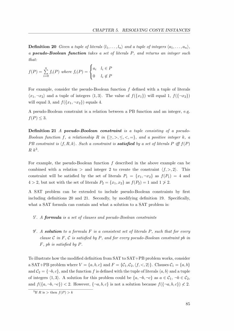
CHAPTER 5. RESOLVING COSYE INSTANCES
Definition 20 Given a tuple of literals 〈l1, . . . , ln〉 and a tuple of integers 〈a1, . . . , an〉,a pseudo-Boolean function takes a set of literals P , and returns an integer such
that:
f(P ) =n∑i=0
fi(P ) where fi(P ) =
ai li ∈ P
0 li 6∈ P
For example, consider the pseudo-Boolean function f defined with a tuple of literals
〈x1,¬x2〉 and a tuple of integers 〈1, 3〉. The value of f(x1) will equal 1, f(¬x2)will equal 3, and f(x1,¬x2) equals 4.
A pseudo-Boolean constraint is a relation between a PB function and an integer, e.g.
f(P ) ≤ 3.
Definition 21 A pseudo-Boolean constraint is a tuple consisting of a pseudo-
Boolean function f , a relationship R in ≥, >,≤, <,=, and a positive integer k, a
PB constraint is 〈f,R, k〉. Such a constraint is satisfied by a set of literals P iff f(P )
R k3.
For example, the pseudo-Boolean function f described in the above example can be
combined with a relation > and integer 2 to create the constraint 〈f,>, 2〉. This
constraint will be satisfied by the set of literals P1 = x1,¬x2 as f(P1) = 4 and
4 > 2, but not with the set of literals P2 = x1, x2 as f(P2) = 1 and 1 6> 2.
A SAT problem can be extended to include pseudo-Boolean constraints by first
including definitions 20 and 21. Secondly, by modifying definition 19. Specifically,
what a SAT formula can contain and what a solution to a SAT problem is:
5′. A formula is a set of clauses and pseudo-Boolean constraints
9′. A solution to a formula F is a consistent set of literals P , such that for every
clause C in F , C is satisfied by P , and for every pseudo-Boolean constraint pb in
F , pb is satisfied by P .
To illustrate how the modified definition from SAT to SAT+PB problem works, consider
a SAT+PB problem where V = a, b, c and F = C1, C2, 〈f,<, 2〉. Clauses C1 = a, band C2 = ¬b, c, and the function f is defined with the tuple of literals 〈a, b〉 and a tuple
of integers 〈1, 3〉. A solution for this problem could be a,¬b,¬c as a ∈ C1, ¬b ∈ C2,and f(a,¬b,¬c) < 2. However, ¬a, b, c is not a solution because f(¬a, b, c) 6< 2.
3If R is > then f(P ) > k
85
CHAPTER 5. RESOLVING COSYE INSTANCES
5.1.2 Boolean Lexicographic Optimization
In order to create a BLO problem, some criteria used to define what properties an
optimal solution have are required. A pseudo-Boolean criterion is defined to either
maximise of minimise the value of a PB function. By composing such criteria together
into a list in order of lexicographic preference, an optimal solution to a BLO problem
can be defined.
Definition 22 A pseudo-Boolean criterion crit is a tuple consisting of a pseudo-
Boolean function f , a relation over integers R that is either < or >, and a SAT+PB
formula I, i.e. crit = 〈f,R, I〉.
The formula I is used to define auxiliary variables. Such variables are used to express
aspects of the problem that are not directly defined in the problems formula.
To describe the use of I, an example is presented where a user wants to minimise the
number different software licences in a component system (to potentially lower legal
fees). This criterion require auxiliary variables l1, . . . , ln, where each variable represents
a licence included in the system. In this example, components a and b are the only
components with licence l1. This means that an iff assignment includes either a or b it
must also include l1, i.e. l1 ⇔ a∨ b. To ensure this constraint is satisfied, the formula I
is defined to include and expansion into the SAT constraints of l1 ⇔ a ∨ b (¬l1, a, b,¬a, l1 and b,¬l1). A PB function f is constructed using the literals 〈l1, . . . , ln〉 and
integers 〈11, . . . , 1n〉. The criterion to minimise the number of licences is defined as
〈f,>, I〉.
BLO uses a list of PB criteria ordered by lexicographic preference to find an optimal
solution. That is, the most preferred criterion to optimise is at the start of the list,
and the least at the end. The lexicographic order is defined : (a, b) is lexicographically
better than (a′, b′) iff a is better than a′ or (a equals a′ and b is better than b′). These
terms are translated to the BLO domain.
Definition 23 Given a SAT+PB formula F , a pseudo-Boolean criteria 〈f,R, I〉, and
two sets of literals P and P ′,
• P and P ′ are equal w.r.t. 〈f,R, I〉 iff P and P ′ are solutions to F ∪ I and
f(P ) = f(P ′).
• P is better than P ′ w.r.t. 〈f,R, I〉 iff P and P ′ are solutions to F ∪ I and f(P ′)
R f(P ).
86
CHAPTER 5. RESOLVING COSYE INSTANCES
Note that both P and P ′ must be solutions to the formula F ∪I, not just the formula F .
This is done to ensure that the auxiliary variables required by the criteria are available.
Also note the relation R that is either < or >, is therefore used to either maximise or
minimise the PB function.
These definitions are used to define the lexicographic order:
Definition 24 Given a formula F , a tuple of PB criteria 〈crit1, . . . , critn〉, and two sets
of literals P and P ′, P is lexicographically better than P ′ w.r.t. to 〈crit1, . . . , critn〉iff there exists an i between 1 and n where for all j < i, P is equal to P ′ w.r.t. to critj
and P is better than P ′ w.r.t. criti.
This means that for a solution to be lexicographically better than another, it must be
better w.r.t. to a PB criterion and at least equal to all criteria that are before it in the
tuple of criteria.
This lexicographic order is then used to define an optimal solution of a BLO problem:
Definition 25 Given a formula F and lexicographically ordered PB criteria 〈crit1, . . . , critn〉an optimal solution is a solution P to F where no other solution P ′ to F exists such
that P ′ is lexicographically greater than P w.r.t. to 〈crit1, . . . , critn〉.
This means that given a BLO problem that consists of:
• A tuple of PB criteria 〈crit1, . . . , critn〉.
• A SAT+PB formula F .
A solution to BLO problem is the optimal solution to F w.r.t. to its PB criteria.
5.1.3 Mapping CoSyE Instance to BLO Problems
Following from the definition of CoSyE in section 3.1, an instance of CoSyE consists of
a series of evolution steps at time ti, where i is from 1 to n. Each step consists of:
• a time ti
• the set of components Cti
• an evolution problem δti ∪ ωti
• an evolution preference order ≺αti−1
87
CHAPTER 5. RESOLVING COSYE INSTANCES
• a previous system αti−1 .
To resolve a CoSyE instance each step is mapped to a BLO problem which consists of
a SAT+PB formula F and PB criteria 〈crit1, . . . , critn〉.
The set of components Cti are variables in the problem, i.e Cti ⊆ Vti . The reason for
this direct use of components as variables, as opposed to mapping, is that it allows PB
criteria to use properties of a component, e.g. a components name. Not all variables in
the problem are components, as auxiliary variables may be required. Each component
variable can then describe two literals, either itself or its negation (definition 19). A
set of such literals are used to describe component systems.
Definition 26 A component system αti−1 is mapped to a set of literals where αti−1 :=
αti−1 ∪ ¬c | c ∈ Cti and c 6∈ αti−1.
A component system αti−1 is mapped to a set of literals that are positive if they are in
the system or negative if they are not.
The reverse mapping, from a set of literals to a component system, is:
Definition 27 A set of literals P is mapped to a component system β such that
β := c | c ∈ Ct and x ∈ P
A component system is the set of components that are not negative in the set of literals.
Note: the mapping from a set of literals to a component system is surjective, and the
mapping from a component system to a set of literals is injective.
The evolution problem δti∪ωti is mapped to the formula F by mapping each constraint
type to a SAT clause or PB constraint:
1. Exclusion: ¬a is mapped to the clause ¬a
2. Conflict: a→ ¬c is mapped to the clause ¬a,¬c
3. Inclusive Disjunction: a1 ∨ . . . ∨ an is mapped to the clause a1, . . . , an
4. Dependence: a→ c1 ∨ . . . ∨ cn is mapped to the clause ¬a, c1, . . . , cn
5. Exactly One: a1 + . . . + an = 1 is mapped to a pseudo-Boolean constraint
〈f,=, 1〉, where f is defined with the tuple of literals 〈a1, . . . , an〉 and the tuple
of natural numbers 〈11, . . . , 1n〉.
88

CHAPTER 5. RESOLVING COSYE INSTANCES
5.1.4 Evolution Preference Order Mapping
The evolution preference order ≺αti−1(as defined in chapter 3) defined with a
lexicographic composition of criteria crit1⊕ . . .⊕ critn can be mapped to a tuple of PB
criteria 〈crit1, . . . , critn〉 by mapping each criterion criti to a PB criterion criti.
A criterion 〈rankα,≤〉 maps to a PB criteria 〈f,R, I〉 iff:
• R equals the strict order of ≤, i.e. if ≤, R is < and if ≥, R is >.
• Given a solution P to formula I, and P maps to the component system β,
f(P ) = rankα(β).
To map an evolution preference order to the PB criteria, it must be defined with the
lexicographically composed criteria. To map a CoSyE criterion to a PB criterion, it
must satisfy the above constraints. This means that:
• Not all evolution preference orders can be described with lexicographically ordered
PB criteria.
• Not all CoSyE criteria can be mapped to PB criteria.
Therefore, the mapping from evolution preference orders to PB criteria is a partial
mapping.
The partial mapping from CoSyE criteria to PB criteria is not presented here. This is
because many of the CoSyE criteria that can be defined are not useful, e.g. a criteria
that maximises the number of components whose name starts with the letter a. Only
specific criteria are mapped to PB criteria, these are presented in the next section.
To further illustrate the mapping from a CoSyE criteria to a PB criteria, an example
is presented. Consider two components a and b, a criterion 〈rankα, <〉 whose ranking
function is defined as:
rankα(β) =
1 a ∈ β or b ∈ β
0 otherwise
This criterion expresses the preference of having either components a or b (or both) in
the system.
Further consider the pseudo-Boolean criterion 〈f,<, I〉. The auxiliary variable x is
defined such that x⇔ a∨b. This variable must be converted to the set of CNF clauses,
and included in I, i.e. I = ¬x, a, b, ¬a, x, ¬b, x. The PB function f is defined
with the tuple of literals 〈x〉 and natural numbers 〈1〉.
89
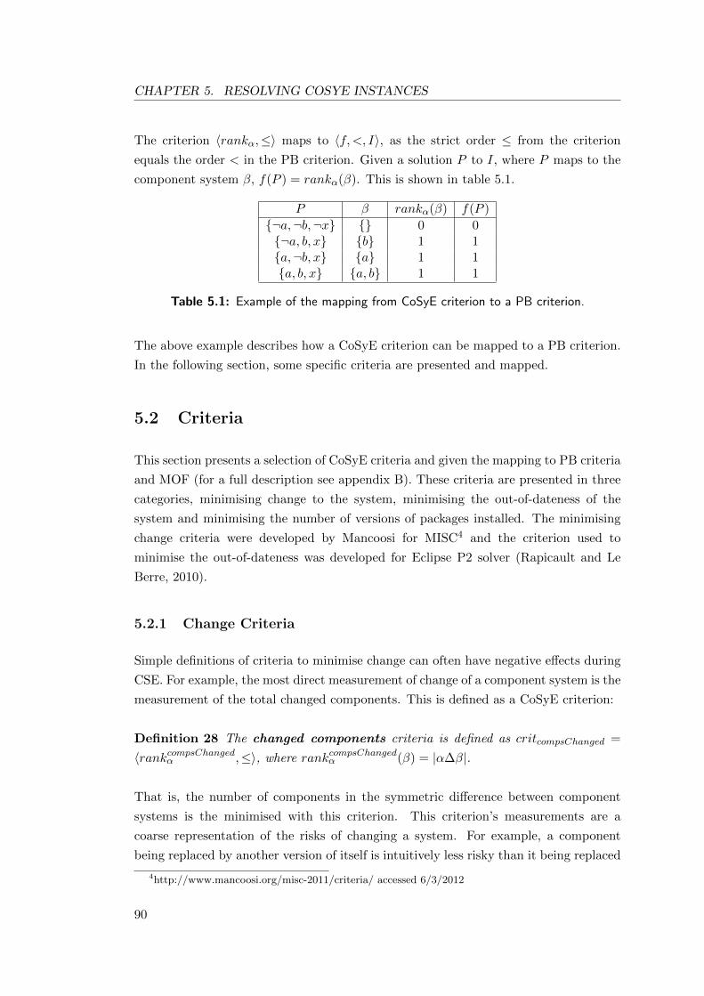
CHAPTER 5. RESOLVING COSYE INSTANCES
The criterion 〈rankα,≤〉 maps to 〈f,<, I〉, as the strict order ≤ from the criterion
equals the order < in the PB criterion. Given a solution P to I, where P maps to the
component system β, f(P ) = rankα(β). This is shown in table 5.1.
P β rankα(β) f(P )
¬a,¬b,¬x 0 0¬a, b, x b 1 1a,¬b, x a 1 1a, b, x a, b 1 1
Table 5.1: Example of the mapping from CoSyE criterion to a PB criterion.
The above example describes how a CoSyE criterion can be mapped to a PB criterion.
In the following section, some specific criteria are presented and mapped.
5.2 Criteria
This section presents a selection of CoSyE criteria and given the mapping to PB criteria
and MOF (for a full description see appendix B). These criteria are presented in three
categories, minimising change to the system, minimising the out-of-dateness of the
system and minimising the number of versions of packages installed. The minimising
change criteria were developed by Mancoosi for MISC4 and the criterion used to
minimise the out-of-dateness was developed for Eclipse P2 solver (Rapicault and Le
Berre, 2010).
5.2.1 Change Criteria
Simple definitions of criteria to minimise change can often have negative effects during
CSE. For example, the most direct measurement of change of a component system is the
measurement of the total changed components. This is defined as a CoSyE criterion:
Definition 28 The changed components criteria is defined as critcompsChanged =
〈rankcompsChangedα ,≤〉, where rankcompsChangedα (β) = |α∆β|.
That is, the number of components in the symmetric difference between component
systems is the minimised with this criterion. This criterion’s measurements are a
coarse representation of the risks of changing a system. For example, a component
being replaced by another version of itself is intuitively less risky than it being replaced
4http://www.mancoosi.org/misc-2011/criteria/ accessed 6/3/2012
90

CHAPTER 5. RESOLVING COSYE INSTANCES
with an entirely different component. Yet using the critcompsChanged criterion, these
would be seen as equivalent changes.
To define a change criterion that takes into account changing between components of
the same name, is less risky, a components name can be considered. For this purpose
the function V is defined:
Definition 29 The function V : 2C × N → 2C takes a set of components α and a
component name n, and returns a set of components with name n that are in α, i.e.
V (α, n) = 〈n′, v〉 | 〈n′, v〉 ∈ α and n′ = n
This function can be used to define a criterion that considers the name of a component:
Definition 30 The change criterion is defined as critchange = 〈rankchangeα ,≤〉, where
rankchangeα (β) = |n | n ∈ N and V (α, n) 6= V (β, n)|.
This criterion can be altered to also consider new and removed component names:
Definition 31 The new criterion is defined as critnew = 〈ranknewα ,≤〉, where
ranknewα (β) = |n | n ∈ N and V (α, n) = ∅ and V (β, n) 6= ∅|.
Definition 32 The removed criterion is defined as critremoved = 〈rankremovedα ,≤〉,where rankremovedα (β) = |n | n ∈ N and V (α, n) 6= ∅ and V (β, n) = ∅|.
The change, new and remove criteria were taken directly from the MISC competitions
definition of criteria.
The mapping between these criteria, PB criteria and MOF are presented in table 5.2.
A full description of the mapping is presented in appendix B.
MOF name CoSyE criterion PB criterion
-changed critchange = 〈rankchangeα ,≤〉 〈fchange, <, Ichange〉-removed critremoved = 〈rankremovedα ,≤〉 〈fremoved, <, Iremoved〉-new critnew = 〈ranknewα ,≤〉 〈fnew, <, Inew〉
Table 5.2: Mapping of the change, removed and new criteria between MOF, CoSyE andPB
5.2.2 Out-of-date Criteria
When changing a component system it is a good idea to select more recent versions
of components, as they keep the system from becoming out-of-date. However, it is a
91
CHAPTER 5. RESOLVING COSYE INSTANCES
difficult task to define an appropriate measurement of how out-of-date a component
system is. This difficulty comes from two properties of component versions must be
considered:
• A version of a component can only be compared to version of another component
with the same name, i.e. given two components 〈n, v〉 and 〈n′, v′〉 comparing v
and v′ is only useful if n = n′.
• The sum of versions is not a useful metric as two lesser versions will not be better
than one greater version, e.g. given components 〈n, 2〉, 〈n, 3〉 and 〈n, 4〉, a system
with only 〈n, 2〉 and 〈n, 3〉 is not better than a system with just 〈n, 4〉.
Not considering these properties when defining criteria could lead to significant
problems.
A useful criterion has been defined in Eclipse P2 that minimises a measurement of
the out-of-dateness of a component name. This measure of out-of-dateness counts the
amount of components that is a greater version than a component currently installed.
It is defined as:
Definition 33 The function uptodatedistance takes a component 〈n, v〉 and a set of
components Ct and returns the number of components with the same name and a greater
version, i.e. uptodatedistance(〈n, v〉,Ct) = |〈n, v′〉 | 〈n, v′〉 ∈ Ct and v′ > v|
A criterion using this measure can then be defined:
Definition 34 Given the set of components Ct, the uptodate distance criterion is
defined as critutdd = 〈rankutddα ,≥〉, where rankutddα (β) =∑
c∈β uptodatedistance(c,Ct).
That is, the measure to be minimised is the number of components that have the
same name, and are a greater version than a component that is currently installed.
This measure depends on the release of new versions to measure out-of-dateness, and
it assumes that components are maintained. If a component is not maintained, and
versions are never released, the component will be measured to never go out-of-date.
Conversely, if a components developer releases versions very quickly, the component
will become quickly out-of-date. These problems can be solved through community
effort to maintain and release components, as is attempted for Debian systems (Barth
et al., 2005).
The mapping between this criterion, MOF and the PB criteria is presented in table 5.3,
with a full description in appendix B.
92

CHAPTER 5. RESOLVING COSYE INSTANCES
MOF CoSyE criterion PB criterion-uptodatedistance critutdd = 〈rankutddα ,≥〉 〈futdd, <, Iutdd〉
Table 5.3: Mapping of the up-to-date distance criterion between MOF, CoSyE and PB
5.2.3 One Version per Package Criteria
As discussed in the previous chapter, the restriction that Ubuntu systems must have
only one version of each package installed is not enforced by the component constraints.
This restriction can however be encouraged by defining a criterion that minimises the
amount of packages with multiple versions.
Definition 35 Given the set of components Ct, the One Version per Package
criterion is defined as critovpp = 〈rankovppα ,≥〉, where rankovppα (β) =∑
n∈N |V (β, n)| >1.
That is, this criteria minimises the number of package names that have more than one
version installed.
The mapping between this criterion, MOF and the PB criteria is presented in table 5.4
with a full description in appendix B.
MOF CoSyE criterion PB criterion-ovpp critovpp = 〈rankovppα ,≥〉 〈fovpp, <, Iovpp〉
Table 5.4: Mapping of the one version per package criterion between MOF, CoSyE andPB
5.3 Solving a BLO Problem
The efficient solving of BLO problems will allow the efficient resolving of CoSyE
instances. This section describes the lexicographic-iterative-strengthening-algorithm
(LIS) to solve BLO problems. This algorithm uses the DPLL algorithm (Davis and
Putnam, 1960; Davis et al., 1962) to find a solution to a SAT+PB formula, and the
iterative strengthening algorithm (Calistri-Yeh, 1994; Le Berre and Parrain, 2010) to
find an optimal solution to a SAT+PB problem given a single PB criterion. This section
also describes how a CoSyE instance is resolved by mapping to BLO problems. The
algorithms presented in this section are described to give an overview of how BLO
problems are solved.
93
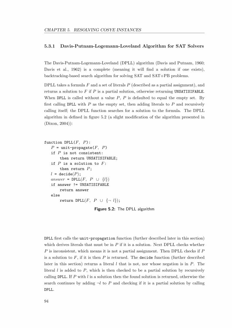
CHAPTER 5. RESOLVING COSYE INSTANCES
5.3.1 Davis-Putnam-Logemann-Loveland Algorithm for SAT Solvers
The Davis-Putnam-Logemann-Loveland (DPLL) algorithm (Davis and Putnam, 1960;
Davis et al., 1962) is a complete (meaning it will find a solution if one exists),
backtracking-based search algorithm for solving SAT and SAT+PB problems.
DPLL takes a formula F and a set of literals P (described as a partial assignment), and
returns a solution to F if P is a partial solution, otherwise returning UNSATISIFABLE.
When DPLL is called without a value P , P is defaulted to equal the empty set. By
first calling DPLL with P as the empty set, then adding literals to P and recursively
calling itself; the DPLL function searches for a solution to the formula. The DPLL
algorithm in defined in figure 5.2 (a slight modification of the algorithm presented in
(Dixon, 2004)):
function DPLL(F , P):P = unit-propagate(F , P)if P is not consistent:
then return UNSATISIFABLE;
if P is a solution to F:then return P;
l = decide(P );answer = DPLL(F , P ∪ l)if answer != UNSATISIFABLE
return answer
else
return DPLL(F , P ∪ ¬ l);
Figure 5.2: The DPLL algorithm
DPLL first calls the unit-propagation function (further described later in this section)
which derives literals that must be in P if it is a solution. Next DPLL checks whether
P is inconsistent, which means it is not a partial assignment. Then DPLL checks if P
is a solution to F , if it is then P is returned. The decide function (further described
later in this section) returns a literal l that is not, nor whose negation is in P . The
literal l is added to P , which is then checked to be a partial solution by recursively
calling DPLL. If P with l is a solution then the found solution is returned, otherwise the
search continues by adding ¬l to P and checking if it is a partial solution by calling
DPLL.
94
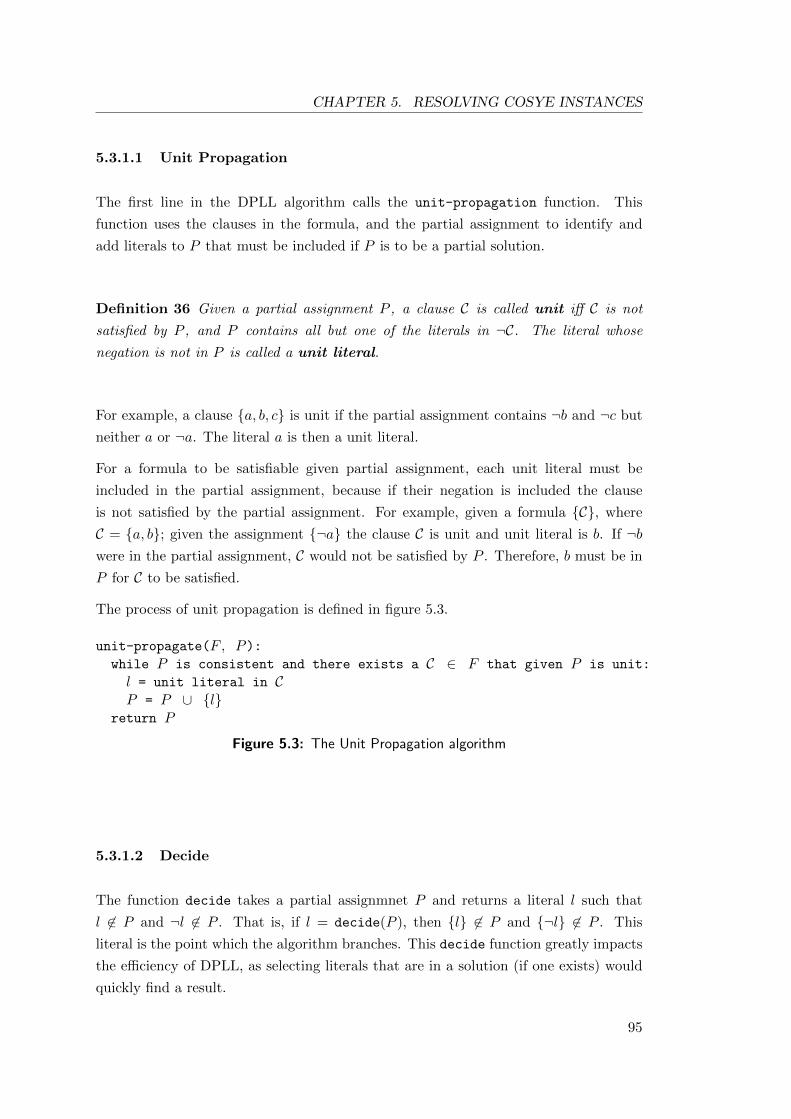
CHAPTER 5. RESOLVING COSYE INSTANCES
5.3.1.1 Unit Propagation
The first line in the DPLL algorithm calls the unit-propagation function. This
function uses the clauses in the formula, and the partial assignment to identify and
add literals to P that must be included if P is to be a partial solution.
Definition 36 Given a partial assignment P , a clause C is called unit iff C is not
satisfied by P , and P contains all but one of the literals in ¬C. The literal whose
negation is not in P is called a unit literal.
For example, a clause a, b, c is unit if the partial assignment contains ¬b and ¬c but
neither a or ¬a. The literal a is then a unit literal.
For a formula to be satisfiable given partial assignment, each unit literal must be
included in the partial assignment, because if their negation is included the clause
is not satisfied by the partial assignment. For example, given a formula C, where
C = a, b; given the assignment ¬a the clause C is unit and unit literal is b. If ¬bwere in the partial assignment, C would not be satisfied by P . Therefore, b must be in
P for C to be satisfied.
The process of unit propagation is defined in figure 5.3.
unit-propagate(F , P):while P is consistent and there exists a C ∈ F that given P is unit:
l = unit literal in CP = P ∪ l
return P
Figure 5.3: The Unit Propagation algorithm
5.3.1.2 Decide
The function decide takes a partial assignmnet P and returns a literal l such that
l 6∈ P and ¬l 6∈ P . That is, if l = decide(P ), then l 6∈ P and ¬l 6∈ P . This
literal is the point which the algorithm branches. This decide function greatly impacts
the efficiency of DPLL, as selecting literals that are in a solution (if one exists) would
quickly find a result.
95
CHAPTER 5. RESOLVING COSYE INSTANCES
5.3.1.3 DPLL Advancements
Though the DPLL algorithm is the basis of many modern SAT solvers, the actual
implementations have been altered to increase efficiency. Some of these improvements
are:
• Conflict learning (Stallman and Sussman, 1976; Sorensson et al., 2009) is a
technique to cache previously tried sets of assignments in order to stop re-solving
the same sub-problems.
• Backjumping (Gaschnig, 1979) is the technique which determines how far to up
the search tree to backtrack when a conflict is found. The higher up the tree the
search “jumps” to, the more of the search space is reduced.
• More efficient unit-propagation through watched literals (Madigan et al., 2001;
Moskewicz et al., 2001).
These advancements have significantly increased the efficiency of current SAT solvers.
5.3.2 Iterative Strengthening
The iterative strengthening algorithm (Calistri-Yeh, 1994; Le Berre and Parrain, 2010)
is an anytime algorithm using constraint satisfaction to iteratively find better solutions
to a SAT+PB formula usings a PB criterion. This algorithm can be used to find optimal
solutions to an evolution problem, given a pseudo-Boolean criterion. This is done by
first finding a solution, then iteratively adding constraints (created using the criterion)
to ensure the next solution found will be better than the previous solution. This is the
strengthening process. Strengthening continues until either the strengthened formula
is found to be unsatisfiable, or the algorithm is interrupted, at which point the best
solution currently found is returned. This algorithm is defined in figure 5.4.
The first action in the iterative-strengthening is to include the formula I that
defines auxiliary variables used by the criterion. This ensures that any solution returned
by DPLL is also a solution to I.
The next action is to check if the formula is satisfiable. This is accomplished by
passing the formula to the DPLL function, and assigning its output to the variable
answer. If the output from DPLL is UNSATISIFABLE, then the algorithm stops and
returns UNSATISIFABLE, as there are no solutions.
The main loop of this algorithm is then defined. The first action in this loop is to
96
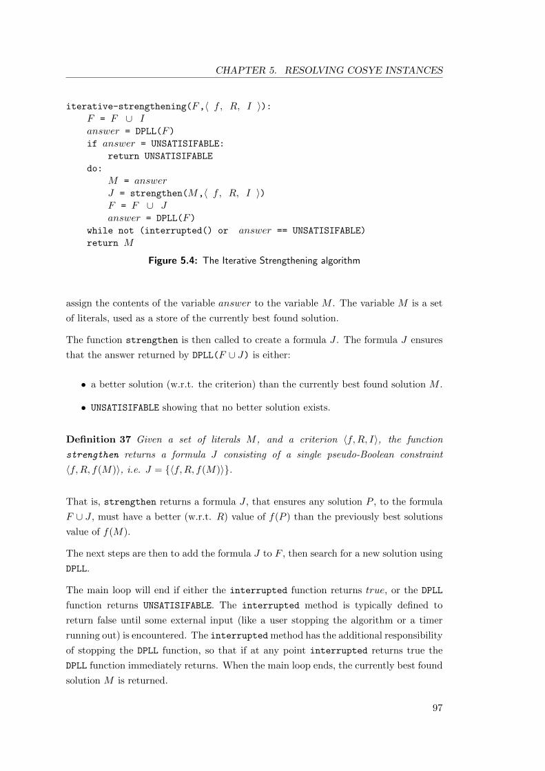
CHAPTER 5. RESOLVING COSYE INSTANCES
iterative-strengthening(F,〈 f, R, I 〉):F = F ∪ Ianswer = DPLL(F)if answer = UNSATISIFABLE:
return UNSATISIFABLE
do:
M = answerJ = strengthen(M,〈 f, R, I 〉)F = F ∪ Janswer = DPLL(F)
while not (interrupted() or answer == UNSATISIFABLE)
return M
Figure 5.4: The Iterative Strengthening algorithm
assign the contents of the variable answer to the variable M . The variable M is a set
of literals, used as a store of the currently best found solution.
The function strengthen is then called to create a formula J . The formula J ensures
that the answer returned by DPLL(F ∪ J) is either:
• a better solution (w.r.t. the criterion) than the currently best found solution M .
• UNSATISIFABLE showing that no better solution exists.
Definition 37 Given a set of literals M , and a criterion 〈f,R, I〉, the function
strengthen returns a formula J consisting of a single pseudo-Boolean constraint
〈f,R, f(M)〉, i.e. J = 〈f,R, f(M)〉.
That is, strengthen returns a formula J , that ensures any solution P , to the formula
F ∪ J , must have a better (w.r.t. R) value of f(P ) than the previously best solutions
value of f(M).
The next steps are then to add the formula J to F , then search for a new solution using
DPLL.
The main loop will end if either the interrupted function returns true, or the DPLL
function returns UNSATISIFABLE. The interrupted method is typically defined to
return false until some external input (like a user stopping the algorithm or a timer
running out) is encountered. The interrupted method has the additional responsibility
of stopping the DPLL function, so that if at any point interrupted returns true the
DPLL function immediately returns. When the main loop ends, the currently best found
solution M is returned.
97
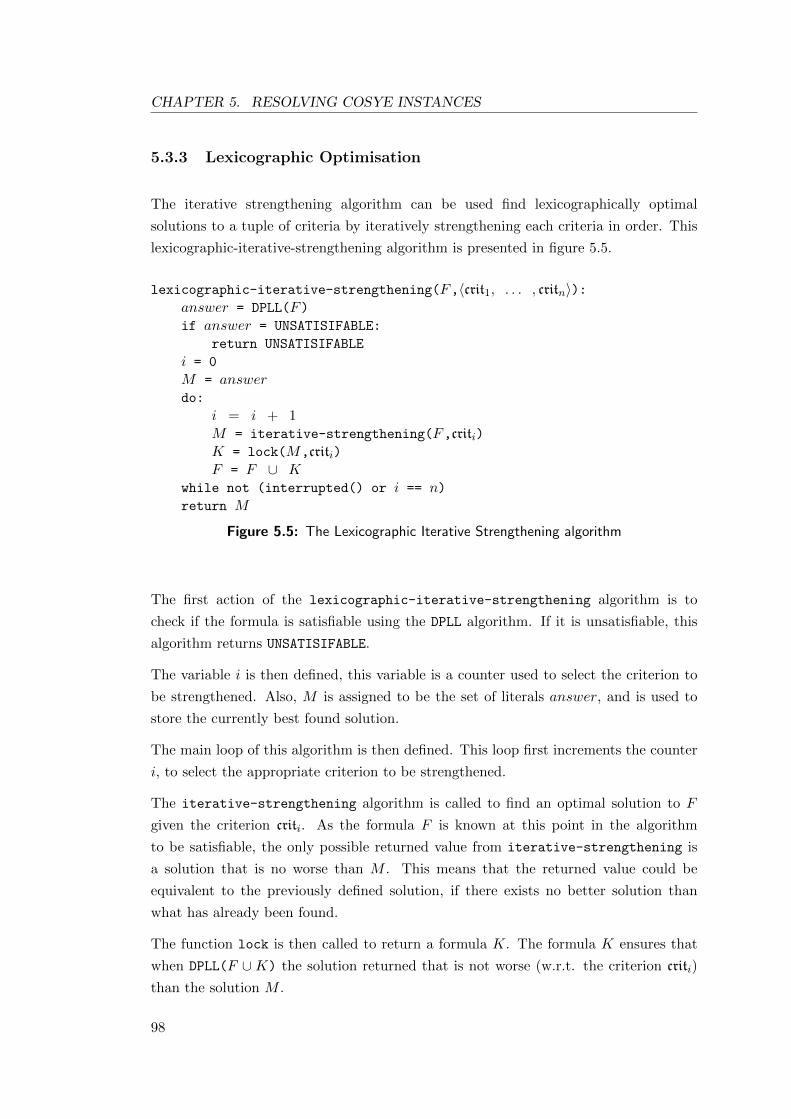
CHAPTER 5. RESOLVING COSYE INSTANCES
5.3.3 Lexicographic Optimisation
The iterative strengthening algorithm can be used find lexicographically optimal
solutions to a tuple of criteria by iteratively strengthening each criteria in order. This
lexicographic-iterative-strengthening algorithm is presented in figure 5.5.
lexicographic-iterative-strengthening(F,〈crit1, . . . , critn〉):answer = DPLL(F)if answer = UNSATISIFABLE:
return UNSATISIFABLE
i = 0
M = answerdo:
i = i + 1M = iterative-strengthening(F,criti)K = lock(M,criti)F = F ∪ K
while not (interrupted() or i == n)return M
Figure 5.5: The Lexicographic Iterative Strengthening algorithm
The first action of the lexicographic-iterative-strengthening algorithm is to
check if the formula is satisfiable using the DPLL algorithm. If it is unsatisfiable, this
algorithm returns UNSATISIFABLE.
The variable i is then defined, this variable is a counter used to select the criterion to
be strengthened. Also, M is assigned to be the set of literals answer, and is used to
store the currently best found solution.
The main loop of this algorithm is then defined. This loop first increments the counter
i, to select the appropriate criterion to be strengthened.
The iterative-strengthening algorithm is called to find an optimal solution to F
given the criterion criti. As the formula F is known at this point in the algorithm
to be satisfiable, the only possible returned value from iterative-strengthening is
a solution that is no worse than M . This means that the returned value could be
equivalent to the previously defined solution, if there exists no better solution than
what has already been found.
The function lock is then called to return a formula K. The formula K ensures that
when DPLL(F ∪K) the solution returned that is not worse (w.r.t. the criterion criti)
than the solution M .
98
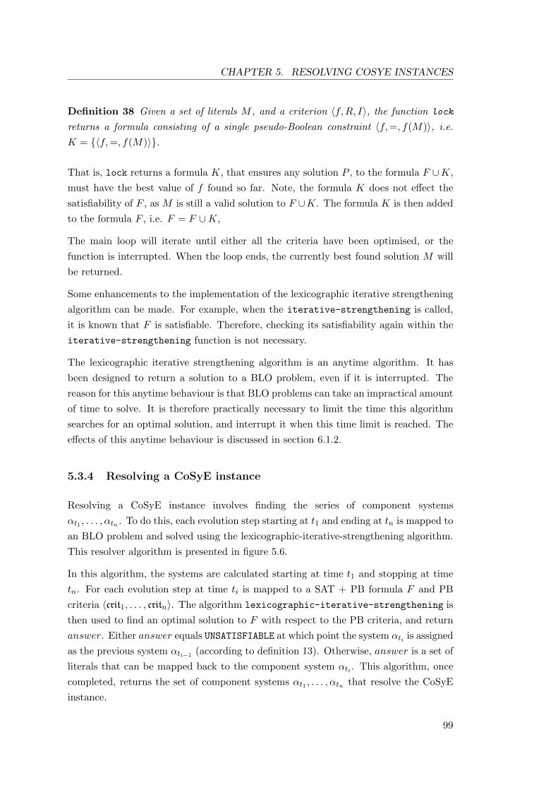
CHAPTER 5. RESOLVING COSYE INSTANCES
Definition 38 Given a set of literals M , and a criterion 〈f,R, I〉, the function lock
returns a formula consisting of a single pseudo-Boolean constraint 〈f,=, f(M)〉, i.e.
K = 〈f,=, f(M)〉.
That is, lock returns a formula K, that ensures any solution P , to the formula F ∪K,
must have the best value of f found so far. Note, the formula K does not effect the
satisfiability of F , as M is still a valid solution to F ∪K. The formula K is then added
to the formula F , i.e. F = F ∪K,
The main loop will iterate until either all the criteria have been optimised, or the
function is interrupted. When the loop ends, the currently best found solution M will
be returned.
Some enhancements to the implementation of the lexicographic iterative strengthening
algorithm can be made. For example, when the iterative-strengthening is called,
it is known that F is satisfiable. Therefore, checking its satisfiability again within the
iterative-strengthening function is not necessary.
The lexicographic iterative strengthening algorithm is an anytime algorithm. It has
been designed to return a solution to a BLO problem, even if it is interrupted. The
reason for this anytime behaviour is that BLO problems can take an impractical amount
of time to solve. It is therefore practically necessary to limit the time this algorithm
searches for an optimal solution, and interrupt it when this time limit is reached. The
effects of this anytime behaviour is discussed in section 6.1.2.
5.3.4 Resolving a CoSyE instance
Resolving a CoSyE instance involves finding the series of component systems
αt1 , . . . , αtn . To do this, each evolution step starting at t1 and ending at tn is mapped to
an BLO problem and solved using the lexicographic-iterative-strengthening algorithm.
This resolver algorithm is presented in figure 5.6.
In this algorithm, the systems are calculated starting at time t1 and stopping at time
tn. For each evolution step at time ti is mapped to a SAT + PB formula F and PB
criteria 〈crit1, . . . , critn〉. The algorithm lexicographic-iterative-strengthening is
then used to find an optimal solution to F with respect to the PB criteria, and return
answer. Either answer equals UNSATISFIABLE at which point the system αti is assigned
as the previous system αti−1 (according to definition 13). Otherwise, answer is a set of
literals that can be mapped back to the component system αti . This algorithm, once
completed, returns the set of component systems αt1 , . . . , αtn that resolve the CoSyE
instance.
99
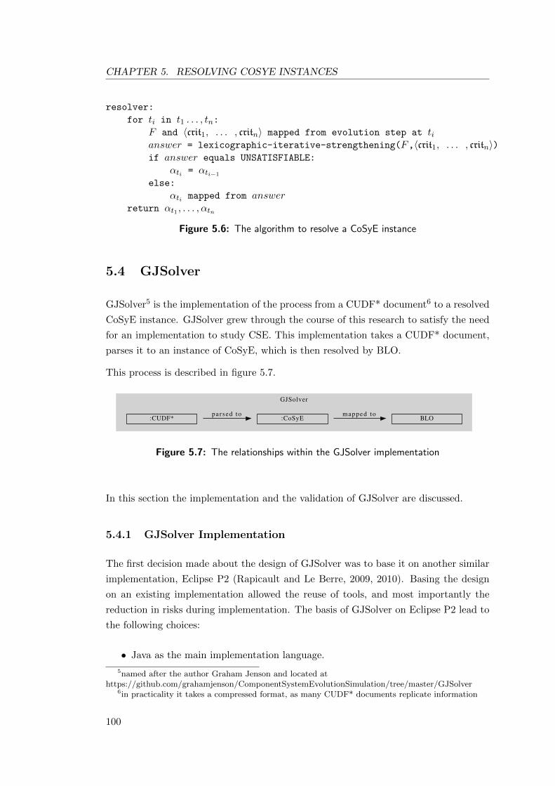
CHAPTER 5. RESOLVING COSYE INSTANCES
resolver:
for ti in t1 . . . , tn:F and 〈crit1, . . . , critn〉 mapped from evolution step at tianswer = lexicographic-iterative-strengthening(F,〈crit1, . . . , critn〉)if answer equals UNSATISFIABLE:
αti = αti−1
else:
αti mapped from answerreturn αt1 , . . . , αtn
Figure 5.6: The algorithm to resolve a CoSyE instance
5.4 GJSolver
GJSolver5 is the implementation of the process from a CUDF* document6 to a resolved
CoSyE instance. GJSolver grew through the course of this research to satisfy the need
for an implementation to study CSE. This implementation takes a CUDF* document,
parses it to an instance of CoSyE, which is then resolved by BLO.
This process is described in figure 5.7.
GJSolver
:CoSyE BLOmapped to
:CUDF*parsed to
Figure 5.7: The relationships within the GJSolver implementation
In this section the implementation and the validation of GJSolver are discussed.
5.4.1 GJSolver Implementation
The first decision made about the design of GJSolver was to base it on another similar
implementation, Eclipse P2 (Rapicault and Le Berre, 2009, 2010). Basing the design
on an existing implementation allowed the reuse of tools, and most importantly the
reduction in risks during implementation. The basis of GJSolver on Eclipse P2 lead to
the following choices:
• Java as the main implementation language.
5named after the author Graham Jenson and located athttps://github.com/grahamjenson/ComponentSystemEvolutionSimulation/tree/master/GJSolver
6in practicality it takes a compressed format, as many CUDF* documents replicate information
100
CHAPTER 5. RESOLVING COSYE INSTANCES
• SAT4J as the core SAT+PB solver.
• Optimisation using PB criteria.
Given Eclipse P2 is designed especially for the OSGi and Eclipse component model and
GJSolver is designed for CUDF*, not all of P2 could be reused. Some of the differences
between Eclipse P2 and GJSolver are:
• No OSGi or Eclipse specific code in GJSolver.
• The internal representation of components is not based on OSGi.
Another important difference between Eclipse P2 and GJSolver is that P2 uses an
aggregated PB function (Joao et al., 2011) that combines all the PB criteria into a
single criterion. P2 then uses this aggregated criterion with the iterative-strengthening
algorithm (further described by Rapicault and Le Berre (2010)) to find an optimal
solution to BLO problems. How P2’s optimisation approach compares to GJSolver’s is
not measured, though a general comparison is presented in Joao et al. (2011).
5.4.1.1 SAT4J
Given the use of SAT4J in GJSolver, a brief background of its development is presented
here.
MiniSAT presented in (Niklas Een, 2004), is a simple SAT solver implementation
written in C, and designed for speed and extensibility. It uses the DPLL-based conflict
driven algorithm as discussed in section 5.2. This solver has become popular and is
the basis of many other SAT solvers due to its open source distribution. This has also
lead to a track in the 2011 SAT competitions7 that deals with only altering MiniSAT
to increase performance. This means that MiniSAT has been repeatedly validated for
performance by third parties across many different SAT problems.
SAT4J (Le Berre and Parrain, 2010) is a re-implementation, and extension, of MiniSAT
in the Java programming language. SAT4J has been extended to efficiently solve a
variety of related problems to SAT, including SAT+PB problems. Due to the easily
modifiable and transparent implementation of SAT4J, it has been able to be adapted
to be used in various domains.
7http://www.satcompetition.org/2011/ accessed 6/3/2012
101
CHAPTER 5. RESOLVING COSYE INSTANCES
5.4.2 Validation of GJSolver
The MISC competition, organised by Mancoosi, is a competition to compare CUDF
solvers by asking them to correctly parse and resolve hundreds of CUDF problems, and
return optimal solutions with respect to various criteria. MISC was created to promote
interest in the problem of changing component systems.
By viewing a CUDF problem as a single evolutionary step in a CUDF* problem,
GJSolver was modified to also solve CUDF problems. Using such a modification,
GJSolver could then be entered into the Mancoosi International Solver Competition
(MISC) competition. GJSolver was entered twice into MISC, firstly in a MISC Live
event, which is an interim competition held during 2011; secondly at the MISC 2011
event8, which is the main competition.
GJSolver was slightly modified to be entered into the MISC competition. The main
modification is encountered when the evolution problem is unsatisfiable. In the
evolution step definition (13) the component system αti−1 is returned if the evolution
problem is unsatisfiable. However, in this case, MISC requires that a file with only the
text FAIL is written to state that no solution was found. This is to correctly score a
solver returning an incorrect solution to an evolution problem, and a solver finding a
problem unsatisfiable.
5.4.2.1 Mancoosi International Solver Competition
To enter GJSolver into MISC the interface and standards defined for this competition
must be followed. How the entered solvers are executed, what environment they are
executed in, and the output required are all important aspects.
The way in which the entered solvers are executed is standardised to allow the
automation of the competition. This standard requires the entered solvers to be able
to be executed on the command line with three arguments, cudfin, cudfout and
criteria. These arguments are defined as:
• cudfin: is a relative path to a CUDF document (as specified in section 3.2) that
describes the problem to be solver.
• cudfout: is a relative path to a non-existent file, which is created by the solver
to output the solution.
8The results for MISC 2011 were announced at the Workshop on Logics for ComponentConfiguration9.
102
CHAPTER 5. RESOLVING COSYE INSTANCES
• criteria: is a Mancoosi optimisation format (as described in section 3.2.3)
description of the criteria to select an optimal solution.
The format of the output file, located at the path defined with cudfout argument, is a
list of packages serialised as a list of stanzas with package and version properties.
The environment in which the solver is executed is a virtual machine running a
GNU/Linux system in a x86 architecture with 1GB of RAM. It contains a Java runtime
environment, allowing the use of Java as a primary language. The time in which the
solver is allowed to run is five minutes, after this time the solver will be forcibly stopped.
This time limit ensures that the competition can be run in an practical time frame.
5.4.2.2 Tracks and Scoring
The MISC 2011 competition is broken down into three possible tracks, where each track
is defined by the criteria used. The first basic track, is “paranoid”, the second more
advanced track is“trendy”, and third track is“user”. Both“paranoid”and“trendy”have
pre-defined criteria, e.g. the “paranoid” tracks criteria in MOF is -removed,-changed.
The “user” track creates unknown criteria from a set of pre-defined criteria, so that
the exact optimisation criteria is unknown before the competition. This means that
“paranoid” and “trendy” can have solvers tailored to their specific criteria, where the
“user” track cannot. The exact criteria that is used for these tracks can be found on
the MISC website10.
For each track, a set of solvers is entered. Each track has a set of evolution problems
defined in CUDF. The solvers for each track are then called to return optimal solutions
for all problems given the tracks criteria.
As MISC competitions were created to compare various solvers, a scoring system was
developed. When a solver is given a CUDF problem and some criteria, the returned
solution falls into one of three classes:
• a real solution is any solution to the CUDF problem.
• no solution occurs when a solver finished without returning a solution. This can
happen because of error, timeout, or there not being a satisfiable solution.
• an incorrect solution occurs when the solver returns an answer that is not a
solution to the CUDF problem.
10http://www.mancoosi.org/misc-2011/criteria/ accessed 12/5/2012
103
CHAPTER 5. RESOLVING COSYE INSTANCES
Given m is the number of solvers that entered into the track, the scoring of a solvers
solution to an individual CUDF problem is as follows:
• a real solution is given 1 point, with an additional 1 point for every solver that
found a better solution.
• for no solution 2×m points are given
• for an incorrect solution 3×m points are given.
This means, if a solver returns an optimal solution to a CUDF problem, it will receive
1 point. However, if other better solutions are returned, then the solver could be given
up to m points.
For each track, all solvers in that track are assigned points based on their solutions to
all problems in that track. For a given track a solvers points are summed to give a final
score. If more than one solver has the same amount of points at the end of a track,
then the time it took for them to find each solution is summed. This total time value
is used as the tie breaker.
5.4.2.3 MISC Live
The MISC Live was entered when GJSolver was only partially implemented. Therefore,
the only track that was possible to enter was the “paranoid” track. The results for
this track11 where promising, though some improvements were necessary. GJSolver’s
deficiencies were identified and corrected.
5.4.2.4 MISC
The main validation of GJSolver was through the MISC 2011 event. In this event
GJSolver was entered into all tracks of this event. The “paranoid” track had a total of
5 solvers, the “trendy” track had a total of 6 solvers, and the “user” track had a total
of 4 solvers. Each track was also entered by the solver which GJSolver is based on,
Eclipse P2, and another efficient solver aspuncud. These two solvers will form the basis
of GJSolver’s comparison.
The scores and the times for each of the track compared to that from Eclipse P2 and
aspuncud are in table 5.5.
11http://mancoosi.org/misc-live/20101126/paranoid/ accessed 6/3/2012
104
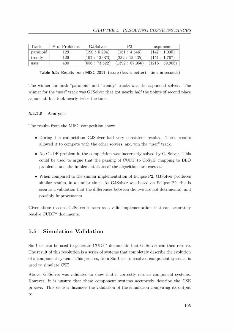
CHAPTER 5. RESOLVING COSYE INSTANCES
Track # of Problems GJSolver P2 aspuncud
paranoid 129 (190 : 5,294) (181 : 4,646) (147 : 1,035)
trendy 129 (197 : 13,073) (232 : 13,435) (151 : 1,767)
user 400 (656 : 73,522) (1392 : 87,956) (1215 : 39,905)
Table 5.5: Results from MISC 2011, (score (less is better) : time in seconds)
The winner for both “paranoid” and “trendy” tracks was the aspuncud solver. The
winner for the “user” track was GJSolver that got nearly half the points of second place
aspuncud, but took nearly twice the time.
5.4.2.5 Analysis
The results from the MISC competition show:
• During the competition GJSolver had very consistent results. These results
allowed it to compete with the other solvers, and win the “user” track.
• No CUDF problem in the competition was incorrectly solved by GJSolver. This
could be used to argue that the parsing of CUDF to CoSyE, mapping to BLO
problems, and the implementations of the algorithms are correct.
• When compared to the similar implementation of Eclipse P2, GJSolver produces
similar results, in a similar time. As GJSolver was based on Eclipse P2, this is
seen as a validation that the differences between the two are not detrimental, and
possibly improvements.
Given these reasons GJSolver is seen as a valid implementation that can accurately
resolve CUDF* documents.
5.5 Simulation Validation
SimUser can be used to generate CUDF* documents that GJSolver can then resolve.
The result of this resolution is a series of systems that completely describe the evolution
of a component system. This process, from SimUser to resolved component systems, is
used to simulate CSE.
Above, GJSolver was validated to show that it correctly returns component systems.
However, it is unsure that these component systems accurately describe the CSE
process. This section discusses the validation of the simulation comparing its output
to:
105
CHAPTER 5. RESOLVING COSYE INSTANCES
• the apt-get logs collected from 19 respondents of the survey.
• a virtual Ubuntu 11.10 system that upgrades everyday over the month of
November 2011.
Both of these comparisons are against systems that use apt-get to alter their systems.
To accurately compare the evolution these systems to the simulated systems, the criteria
used by apt-get to upgrade and install systems must be defined in MOF.
To upgrade a system the apt-get manual12 states the following:
upgrade is used to install the newest versions of all packages currently
installed on the system [. . . ] under no circumstances are currently installed
packages removed, or packages not already installed retrieved and installed.
To represent the apt-get upgrade criteria in MOF -removed,-new,-uptodatedistance13
is used. The hard constraints in apt-get to never remove or install new packages are
softened when using this criteria. However, they have been made more important in
the lexicographical order to encourage the GJSolver to not remove or add packages.
When installing a package it is assumed that apt-get will try to select the most recent
version component while minimising change. This has lead to using the MOF criteria
-ovpp,-removed,-changed,-uptodatedistance to represent the apt-get criteria for
installing a component. The first criterion -ovpp minimises the number of package
with more than one package installed. -removed is the second criterion, as removing
a package from a system is seen as more risky than installing a new package. The
final two criteria describe that minimising change to the system is more important that
installing a more recent version of a component.
5.5.1 Comparison to apt-get Logs
The respondents to the user survey (as discussed in chapter 4) submitted 19 logs that
record their use of apt-get. These logs were parsed and the requests the users made to
install components where studied. Particularly the change that each request to install
had on their system. These results were compared to the simulation by selecting the
200 most likely packages to be installed, and installing them on the first day of the
simulation. The results are presented in table 5.6.
12http://linux.die.net/man/8/apt-get13the criterion -ovpp is not necessary in the upgrade criteria as only allowing one package to be
installed is a hard constraint of the upgrade request
106
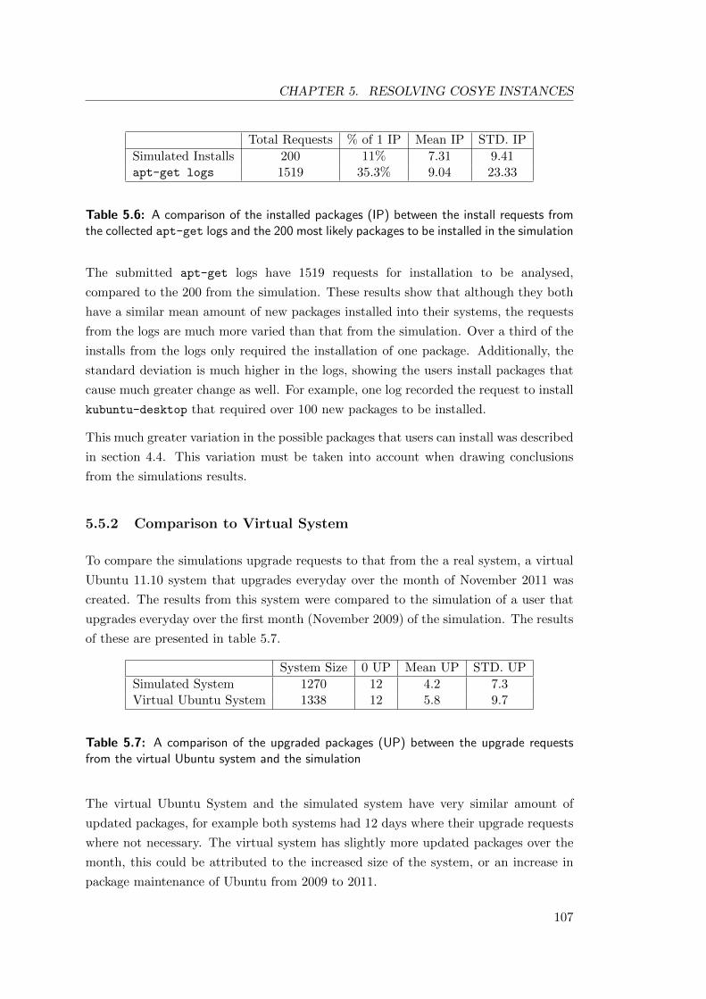
CHAPTER 5. RESOLVING COSYE INSTANCES
Total Requests % of 1 IP Mean IP STD. IP
Simulated Installs 200 11% 7.31 9.41apt-get logs 1519 35.3% 9.04 23.33
Table 5.6: A comparison of the installed packages (IP) between the install requests fromthe collected apt-get logs and the 200 most likely packages to be installed in the simulation
The submitted apt-get logs have 1519 requests for installation to be analysed,
compared to the 200 from the simulation. These results show that although they both
have a similar mean amount of new packages installed into their systems, the requests
from the logs are much more varied than that from the simulation. Over a third of the
installs from the logs only required the installation of one package. Additionally, the
standard deviation is much higher in the logs, showing the users install packages that
cause much greater change as well. For example, one log recorded the request to install
kubuntu-desktop that required over 100 new packages to be installed.
This much greater variation in the possible packages that users can install was described
in section 4.4. This variation must be taken into account when drawing conclusions
from the simulations results.
5.5.2 Comparison to Virtual System
To compare the simulations upgrade requests to that from the a real system, a virtual
Ubuntu 11.10 system that upgrades everyday over the month of November 2011 was
created. The results from this system were compared to the simulation of a user that
upgrades everyday over the first month (November 2009) of the simulation. The results
of these are presented in table 5.7.
System Size 0 UP Mean UP STD. UP
Simulated System 1270 12 4.2 7.3Virtual Ubuntu System 1338 12 5.8 9.7
Table 5.7: A comparison of the upgraded packages (UP) between the upgrade requestsfrom the virtual Ubuntu system and the simulation
The virtual Ubuntu System and the simulated system have very similar amount of
updated packages, for example both systems had 12 days where their upgrade requests
where not necessary. The virtual system has slightly more updated packages over the
month, this could be attributed to the increased size of the system, or an increase in
package maintenance of Ubuntu from 2009 to 2011.
107
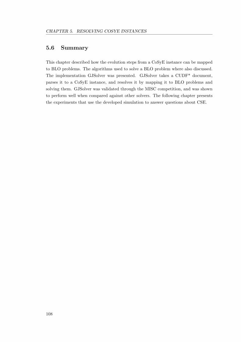
CHAPTER 5. RESOLVING COSYE INSTANCES
5.6 Summary
This chapter described how the evolution steps from a CoSyE instance can be mapped
to BLO problems. The algorithms used to solve a BLO problem where also discussed.
The implementation GJSolver was presented. GJSolver takes a CUDF* document,
parses it to a CoSyE instance, and resolves it by mapping it to BLO problems and
solving them. GJSolver was validated through the MISC competition, and was shown
to perform well when compared against other solvers. The following chapter presents
the experiments that use the developed simulation to answer questions about CSE.
108
Chapter 6
Experiments, Results and
Analysis
Experiment is the sole judge of scientific truth.
The Feynman Lectures on Physics, Introduction, Richard Feynman, 1961.
Previously the models and the implementation used to simulate CSE have been
described. The SimUser model is used to create CUDF* documents given the
probabilities a user will request to upgrade and install components, and the criteria used
to accomplish these requests. These documents describe the evolution of an Ubuntu
system for a year starting on October 30th 2009. GJSolver can be used to resolve the
exact evolution of the system described by such a document. This process of describing
a user in SimUser, generating CUDF* documents, then resolving the evolution is used
to explore CSE.
This chapter presents experiments and results to study the effects of CSE. The specific
effects that are focused on are the change made to the system, and the out-of-dateness
of the system during evolution. This exploration is accomplished through trying to
answer the questions:
1. What consequences do a user’s choices have on their system (i.e. their
probabilities to upgrade u and install i) when using the apt-get criteria?
2. Can the out-of-dateness of a system be reduced?
3. Can the total change of a system be reduced?
4. How do the systems of realistic users evolve?
109
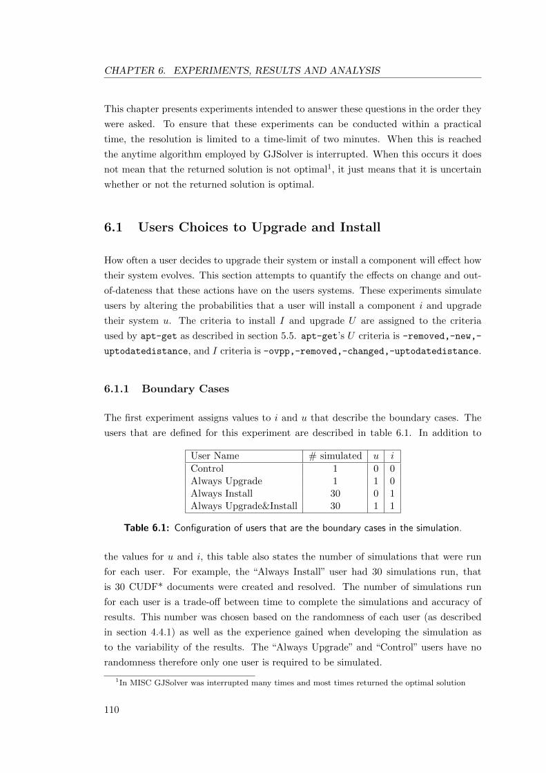
CHAPTER 6. EXPERIMENTS, RESULTS AND ANALYSIS
This chapter presents experiments intended to answer these questions in the order they
were asked. To ensure that these experiments can be conducted within a practical
time, the resolution is limited to a time-limit of two minutes. When this is reached
the anytime algorithm employed by GJSolver is interrupted. When this occurs it does
not mean that the returned solution is not optimal1, it just means that it is uncertain
whether or not the returned solution is optimal.
6.1 Users Choices to Upgrade and Install
How often a user decides to upgrade their system or install a component will effect how
their system evolves. This section attempts to quantify the effects on change and out-
of-dateness that these actions have on the users systems. These experiments simulate
users by altering the probabilities that a user will install a component i and upgrade
their system u. The criteria to install I and upgrade U are assigned to the criteria
used by apt-get as described in section 5.5. apt-get’s U criteria is -removed,-new,-
uptodatedistance, and I criteria is -ovpp,-removed,-changed,-uptodatedistance.
6.1.1 Boundary Cases
The first experiment assigns values to i and u that describe the boundary cases. The
users that are defined for this experiment are described in table 6.1. In addition to
User Name # simulated u i
Control 1 0 0Always Upgrade 1 1 0Always Install 30 0 1Always Upgrade&Install 30 1 1
Table 6.1: Configuration of users that are the boundary cases in the simulation.
the values for u and i, this table also states the number of simulations that were run
for each user. For example, the “Always Install” user had 30 simulations run, that
is 30 CUDF* documents were created and resolved. The number of simulations run
for each user is a trade-off between time to complete the simulations and accuracy of
results. This number was chosen based on the randomness of each user (as described
in section 4.4.1) as well as the experience gained when developing the simulation as
to the variability of the results. The “Always Upgrade” and “Control” users have no
randomness therefore only one user is required to be simulated.
1In MISC GJSolver was interrupted many times and most times returned the optimal solution
110
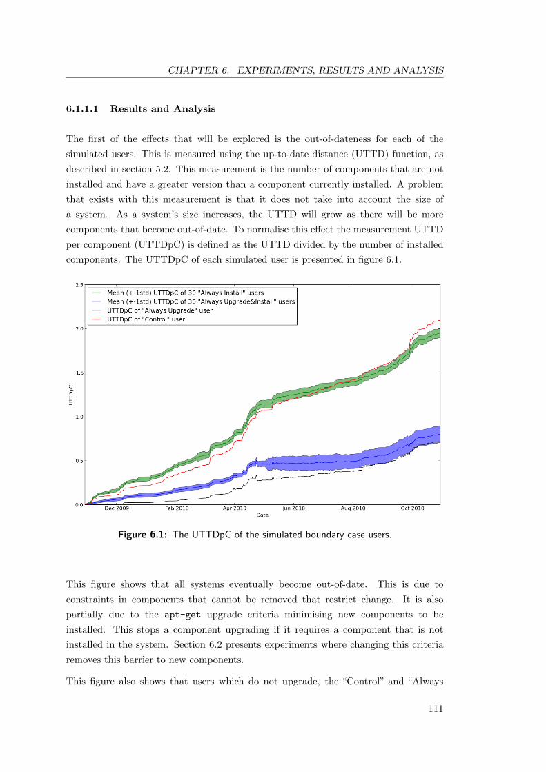
CHAPTER 6. EXPERIMENTS, RESULTS AND ANALYSIS
6.1.1.1 Results and Analysis
The first of the effects that will be explored is the out-of-dateness for each of the
simulated users. This is measured using the up-to-date distance (UTTD) function, as
described in section 5.2. This measurement is the number of components that are not
installed and have a greater version than a component currently installed. A problem
that exists with this measurement is that it does not take into account the size of
a system. As a system’s size increases, the UTTD will grow as there will be more
components that become out-of-date. To normalise this effect the measurement UTTD
per component (UTTDpC) is defined as the UTTD divided by the number of installed
components. The UTTDpC of each simulated user is presented in figure 6.1.
Figure 6.1: The UTTDpC of the simulated boundary case users.
This figure shows that all systems eventually become out-of-date. This is due to
constraints in components that cannot be removed that restrict change. It is also
partially due to the apt-get upgrade criteria minimising new components to be
installed. This stops a component upgrading if it requires a component that is not
installed in the system. Section 6.2 presents experiments where changing this criteria
removes this barrier to new components.
This figure also shows that users which do not upgrade, the “Control” and “Always
111

CHAPTER 6. EXPERIMENTS, RESULTS AND ANALYSIS
Install” users, become nearly three times more out-of-date than users that upgrade.
The speed at which systems become out-of-date increases over the months between
March and May 2010. The reason for this is likely due to the increased development
effort because of the Ubuntu 10.04 release in April 2010. The users that upgrade are
less affected by this release as they are installing newer component versions.
The rate of change of the “Control” users UTTDpC is the rate at which components
evolve. This is because the faster versions of a component are released, the more
the “Control” user becomes out-of-date. As this user will never upgrade its UTTD is
increased by one for every new component release.
The effect of the normalisation of UTTD can also be seen in this figure. The “Control”
and “Always Install” users, and the “Always Upgrade” and “Always Upgrade&Install”
users have similar UTTDpC over the year. This normalisation means that the install
variable i has little effect on the UTTDpC of a component system.
The next effect measured is how much change each simulated system went through
during evolution. To measure change the “change” function as described in section 5.2
is used. The total change, i.e. the sum of all change a system has to date, is presented
in figure 6.2.
Figure 6.2: The total change of the simulated boundary case users.
As was predicted above, this figure shows that there is an increase in change during
112
CHAPTER 6. EXPERIMENTS, RESULTS AND ANALYSIS
the release of Ubuntu 10.04 for users that upgrade their systems. During the months of
March, April and May of 2010 the “Always Upgrade” user had a mean of 266 changes
per month. All other months they had a mean of 105 changes per month. This is
a more than 250% increase in change over the months of the release. This increased
change cannot be seen in the “Always Install” users as they will not change in response
to newer versions.
The effect of reuse of components can be most seen when examining the“Always Install”
users. Initially, these user’s systems change quickly, then after a month the rate of
change decreases. This is measured by looking at the mean change per day; during
the first month 4.9 components are changed per day, where in the final 11 months 3.0
components are changed per day. After further investigation this reduction in change is
explained due to the common reuse of a few components like libaudio2 and libqt3-
mt. Many components depend on these components, and are therefore often installed
in the first month. After this installation they are no longer required to be added so the
future change is reduced. If this reuse did not exist, the rate of change would remain
near 4.9 components per day, resulting in an estimated total change of 1788.5 over a
year. Reuse then saves an estimated 650 changes over the year.
The “Always Upgrade&Install” users changes more than the combined amount
of “Always Upgrade” and “Always Install” changes. The total change of the
“Always Upgrade” user is 1655, the “Always Install” user is 1137 and the “Always
Upgrade&Install” user is 3482. This shows that a user that upgrades and installs
changes more than 700 components than the combined amount changed by just
installing and just upgrading. The additional change is due to the installed components
increasing the amount of components to be upgraded.
6.1.2 Failures
These initial experiments are the most extreme users that can be simulated. This means
phenomena that occur rarely are most observable in these simulations. For this reason,
these simulations were chosen to be closely inspected for various failures.
Two types of failure were observed in the results of these simulations:
1. Hard Failure: Where a request has no solution, therefore no change is made to
the system.
2. Soft Failure: The request is satisfied, however the search was interrupted and
the best solution found at that time was returned.
113
CHAPTER 6. EXPERIMENTS, RESULTS AND ANALYSIS
Additionally, a notable hard failure was observed, the Multi-component Failure
occurs when multiple components must be installed to satisfy a request.
All these failures are directly caused by, or are a result of an install request. The failures
and the rates they occur are therefore a product of the selection of components to be
installed. The validity of this aspect of the simulation is discussed in section 4.4.
6.1.2.1 Hard Failures
Hard failures where observed to occur in 12 of the “Always Install” users, 12 of the
“Always Upgrade&Install” users, and never in the “Always Upgrade” user. Only 40
requests hard failed over these 24 simulated users with hard failures. All hard failures,
except those that are multi-component failures, were failed install requests. Given each
“Always Install” user has 365 requests and each “Always Upgrade&Install” user has 730
requests, and 30 users of each type were simulated, the chance for a request to fail is just
over 0.12%. The chance for a hard failure to occur is extremely low in this simulation.
Due to the rarity of these hard failures, the specific reasons for hard failures are not
further explored.
An interesting failure occurred when the situation arose that installing the package
chromium-browser required two versions of the package libc6 to be installed. This
lead to the following upgrade request to be unsatisfiable, and the following install
request to remove chromium-browser and upgrade to the newest version of libc6.
This instance, although rare, shows the case that at some points the hard constraint
that Debian enforces to have only one version of each component installed, can restrict
the user.
6.1.2.2 Soft Failures
Soft failures are called “soft” because the request that causes them succeeds, however
the search failed to finish. This occurs when the time-limit of two minutes is reached,
and the any-time algorithm is interrupted. Of the 33215 requests during the simulation
of the users defined in table 6.1, only 900 requests suffered soft failures. This is less than
3%. After looking at the results returned by these 900 requests, only 8 were determined
to be detrimental to the simulation. Each of these 8 requests caused more than 100
components in the system to be removed in order to be satisfied. This is due to the
criterion -removed not being fully optimised before being interrupted. There are two
interesting points that were observed with these 8 requests:
1. seven of them occurred during the Ubuntu 10.04 release month of April 2010.
114
CHAPTER 6. EXPERIMENTS, RESULTS AND ANALYSIS
The remainder of the 892 soft failures are evenly distributed over the year.
2. five times the component that was requested to be installed was removed by the
following requests.
The first point implies that these detrimental soft-failures occur because of the increased
release of components during the Ubuntu release. The second point implies that the
components themselves are over constrained and thus removed in future systems. The
effect of these detrimental soft failures can be seen in figure 6.2 where the standard
deviation of change for both “Always Install” and “Always Upgrade&Install” users
increases after the Ubuntu 10.04 release. Given that only 8 such failures occurred,
this is seen as a minor impact on the validity of the simulation. These failures may
be reduced or removed by increasing the time before the algorithm is interrupted, or
by using more powerful hardware to perform the simulations. In all other experiments
detrimental soft failures are searched for, however none were found.
6.1.3 Upgrade Probability Effects
The effect of a user upgrading their system can be measured by altering the probability
they upgrade. The users simulated are described in table 6.2. These users are compared
User Name # simulated u i
Upgrade once a month 10 0.03 (1/30) 0Upgrade twice a month 10 0.06 (1/15) 0Upgrade once a week 10 0.14 (1/7) 0Upgrade twice a week 10 0.29 (1/3.5) 0
Table 6.2: Configuration of users with variable probability to upgrade.
to the “Always Upgrade” user described in table 6.1. The up-to-date distance per
component for these users is compared in figure 6.3. This figure shows that upgrading
less frequently has it’s greatest effect over the release of the Ubuntu 10.04. This is
most noticeable in the “Upgrade once a month” users. The increased release of newer
versions of components makes systems that do not frequently upgrade quickly become
out of date.
The mean UTTDpC of the simulated users plotted against their frequency (1/u) of
upgrading is presented in figure 6.4. The figure shows the mean UTTDpC of “Always
Upgrade” is 0.258 and the “Upgrade twice a week” users’ mean is 0.267. This is a
difference of 0.009 UTTDpC. This difference can be illustrated with an example: given
a system of 1000 components and a user that upgrades twice a week, they will have on
average 9 components more out-of-date than if they upgraded every day. This figure
115
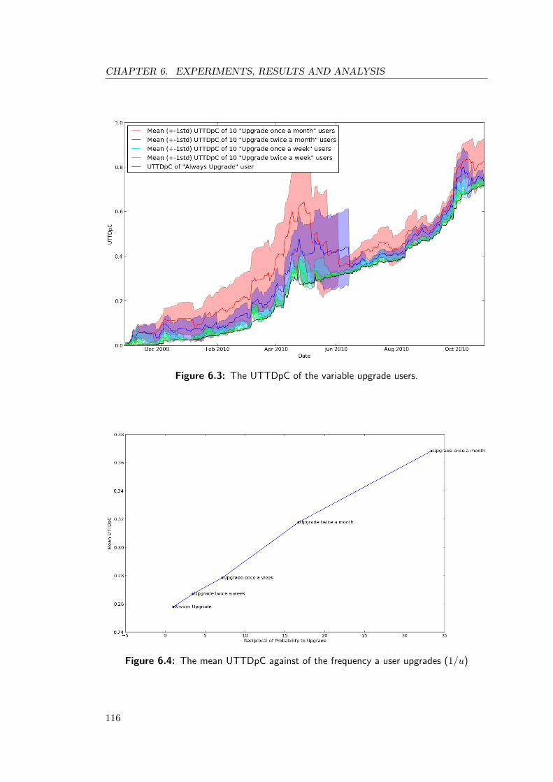
CHAPTER 6. EXPERIMENTS, RESULTS AND ANALYSIS
Figure 6.3: The UTTDpC of the variable upgrade users.
Figure 6.4: The mean UTTDpC against of the frequency a user upgrades (1/u)
116
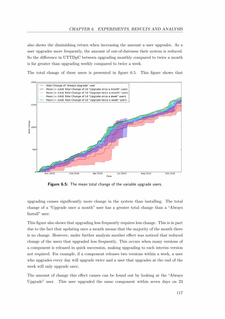
CHAPTER 6. EXPERIMENTS, RESULTS AND ANALYSIS
also shows the diminishing return when increasing the amount a user upgrades. As a
user upgrades more frequently, the amount of out-of-dateness their system is reduced.
So the difference in UTTDpC between upgrading monthly compared to twice a month
is far greater than upgrading weekly compared to twice a week.
The total change of these users is presented in figure 6.5. This figure shows that
Figure 6.5: The mean total change of the variable upgrade users.
upgrading causes significantly more change in the system than installing. The total
change of a “Upgrade once a month” user has a greater total change than a “Always
Install” user.
This figure also shows that upgrading less frequently requires less change. This is in part
due to the fact that updating once a month means that the majority of the month there
is no change. However, under further analysis another effect was noticed that reduced
change of the users that upgraded less frequently. This occurs when many versions of
a component is released in quick succession, making upgrading to each interim version
not required. For example, if a component releases two versions within a week, a user
who upgrades every day will upgrade twice and a user that upgrades at the end of the
week will only upgrade once.
The amount of change this effect causes can be found out by looking at the “Always
Upgrade” user. This user upgraded the same component within seven days on 23
117
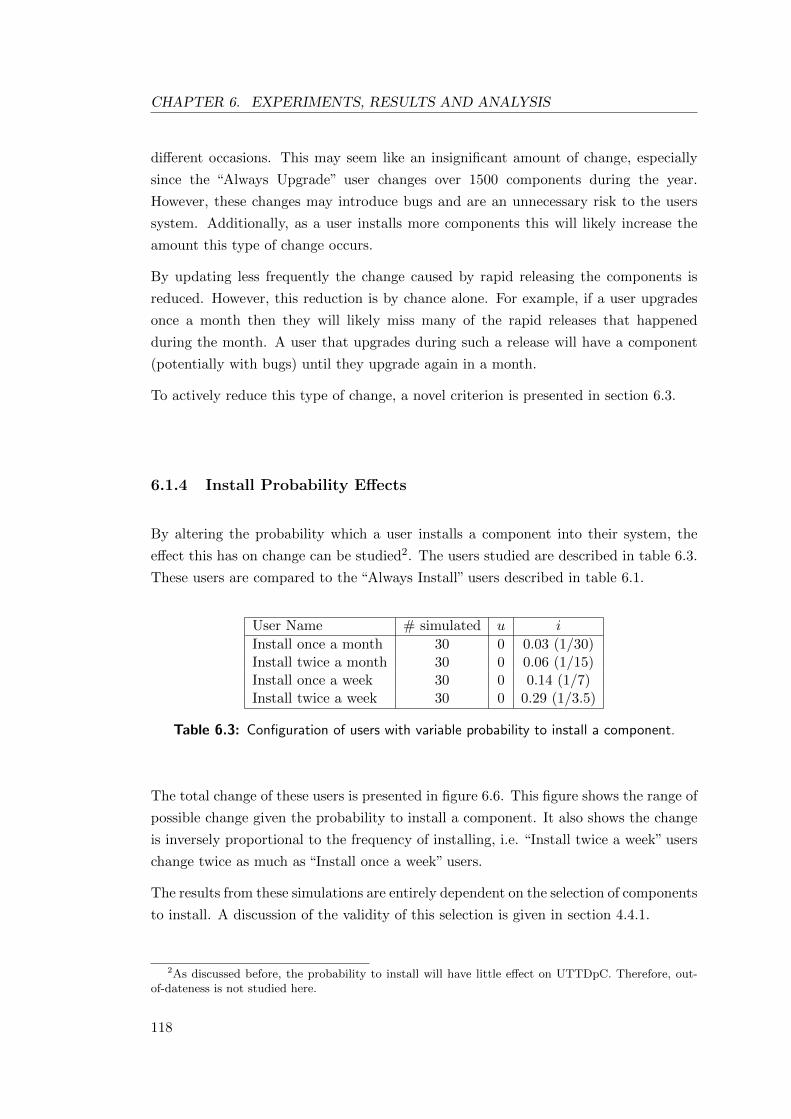
CHAPTER 6. EXPERIMENTS, RESULTS AND ANALYSIS
different occasions. This may seem like an insignificant amount of change, especially
since the “Always Upgrade” user changes over 1500 components during the year.
However, these changes may introduce bugs and are an unnecessary risk to the users
system. Additionally, as a user installs more components this will likely increase the
amount this type of change occurs.
By updating less frequently the change caused by rapid releasing the components is
reduced. However, this reduction is by chance alone. For example, if a user upgrades
once a month then they will likely miss many of the rapid releases that happened
during the month. A user that upgrades during such a release will have a component
(potentially with bugs) until they upgrade again in a month.
To actively reduce this type of change, a novel criterion is presented in section 6.3.
6.1.4 Install Probability Effects
By altering the probability which a user installs a component into their system, the
effect this has on change can be studied2. The users studied are described in table 6.3.
These users are compared to the “Always Install” users described in table 6.1.
User Name # simulated u i
Install once a month 30 0 0.03 (1/30)Install twice a month 30 0 0.06 (1/15)Install once a week 30 0 0.14 (1/7)Install twice a week 30 0 0.29 (1/3.5)
Table 6.3: Configuration of users with variable probability to install a component.
The total change of these users is presented in figure 6.6. This figure shows the range of
possible change given the probability to install a component. It also shows the change
is inversely proportional to the frequency of installing, i.e. “Install twice a week” users
change twice as much as “Install once a week” users.
The results from these simulations are entirely dependent on the selection of components
to install. A discussion of the validity of this selection is given in section 4.4.1.
2As discussed before, the probability to install will have little effect on UTTDpC. Therefore, out-of-dateness is not studied here.
118
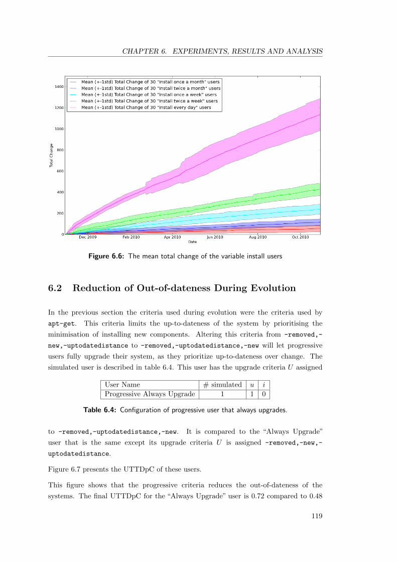
CHAPTER 6. EXPERIMENTS, RESULTS AND ANALYSIS
Figure 6.6: The mean total change of the variable install users
6.2 Reduction of Out-of-dateness During Evolution
In the previous section the criteria used during evolution were the criteria used by
apt-get. This criteria limits the up-to-dateness of the system by prioritising the
minimisation of installing new components. Altering this criteria from -removed,-
new,-uptodatedistance to -removed,-uptodatedistance,-new will let progressive
users fully upgrade their system, as they prioritize up-to-dateness over change. The
simulated user is described in table 6.4. This user has the upgrade criteria U assigned
User Name # simulated u i
Progressive Always Upgrade 1 1 0
Table 6.4: Configuration of progressive user that always upgrades.
to -removed,-uptodatedistance,-new. It is compared to the “Always Upgrade”
user that is the same except its upgrade criteria U is assigned -removed,-new,-
uptodatedistance.
Figure 6.7 presents the UTTDpC of these users.
This figure shows that the progressive criteria reduces the out-of-dateness of the
systems. The final UTTDpC for the “Always Upgrade” user is 0.72 compared to 0.48
119

CHAPTER 6. EXPERIMENTS, RESULTS AND ANALYSIS
Figure 6.7: The UTTDpC of the simulated progressive user.
of the “Progressive Always Upgrade” user. That is, a user who upgrades with the
progressive criteira will have a system that is 24% less out-of-date.
The UTTDpC of these systems is most differentiated during the release of Ubuntu 10.04.
At this time new versions of components are being released quickly. The “Progressive
Always Upgrade” user can upgrade these components if they require new components
to be installed where the “Always Upgrade” user cannot.
These are promising results, showing that it is possible to reduce the out-of-dateness of
a system. However, this comes at the cost of increased change. This additional change
comes from the 90 new components that the progressive change installs. These new
components are also upgraded 258 times throughout the year. The total additional
change when using a progressive user is therefore 348 changes over a year.
When a user upgrades their system with the progressive upgrade criteria at the end of
the year their system is 24% less out-of-date at the cost of an additional 348 changes.
Users that prefer to have an up-to-date system may favour this criteria over the apt-get
criteria. This criteria is further simulated in section 6.4.
120
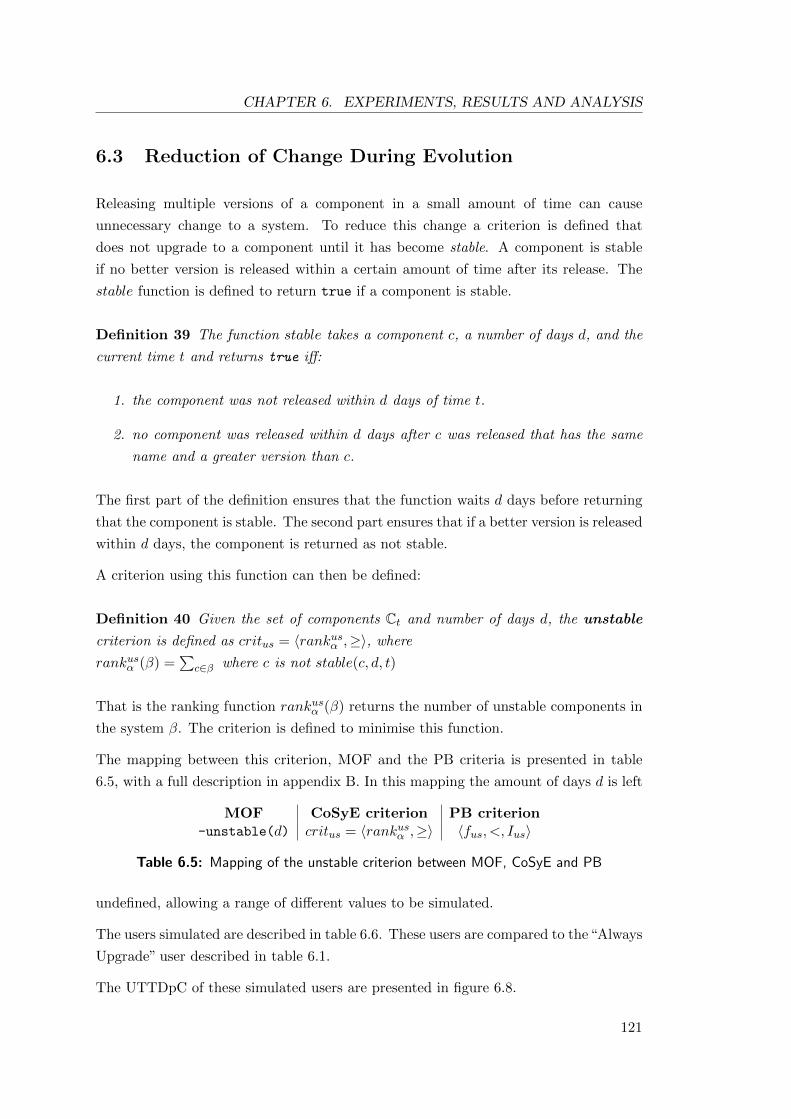
CHAPTER 6. EXPERIMENTS, RESULTS AND ANALYSIS
6.3 Reduction of Change During Evolution
Releasing multiple versions of a component in a small amount of time can cause
unnecessary change to a system. To reduce this change a criterion is defined that
does not upgrade to a component until it has become stable. A component is stable
if no better version is released within a certain amount of time after its release. The
stable function is defined to return true if a component is stable.
Definition 39 The function stable takes a component c, a number of days d, and the
current time t and returns true iff:
1. the component was not released within d days of time t.
2. no component was released within d days after c was released that has the same
name and a greater version than c.
The first part of the definition ensures that the function waits d days before returning
that the component is stable. The second part ensures that if a better version is released
within d days, the component is returned as not stable.
A criterion using this function can then be defined:
Definition 40 Given the set of components Ct and number of days d, the unstable
criterion is defined as critus = 〈rankusα ,≥〉, where
rankusα (β) =∑
c∈β where c is not stable(c, d, t)
That is the ranking function rankusα (β) returns the number of unstable components in
the system β. The criterion is defined to minimise this function.
The mapping between this criterion, MOF and the PB criteria is presented in table
6.5, with a full description in appendix B. In this mapping the amount of days d is left
MOF CoSyE criterion PB criterion-unstable(d) critus = 〈rankusα ,≥〉 〈fus, <, Ius〉
Table 6.5: Mapping of the unstable criterion between MOF, CoSyE and PB
undefined, allowing a range of different values to be simulated.
The users simulated are described in table 6.6. These users are compared to the“Always
Upgrade” user described in table 6.1.
The UTTDpC of these simulated users are presented in figure 6.8.
121
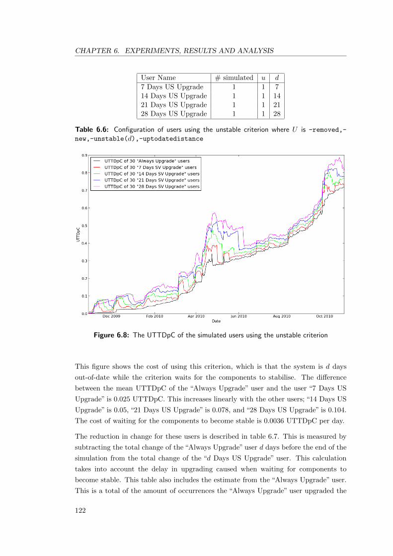
CHAPTER 6. EXPERIMENTS, RESULTS AND ANALYSIS
User Name # simulated u d
7 Days US Upgrade 1 1 714 Days US Upgrade 1 1 1421 Days US Upgrade 1 1 2128 Days US Upgrade 1 1 28
Table 6.6: Configuration of users using the unstable criterion where U is -removed,-
new,-unstable(d),-uptodatedistance
Figure 6.8: The UTTDpC of the simulated users using the unstable criterion
This figure shows the cost of using this criterion, which is that the system is d days
out-of-date while the criterion waits for the components to stabilise. The difference
between the mean UTTDpC of the “Always Upgrade” user and the user “7 Days US
Upgrade” is 0.025 UTTDpC. This increases linearly with the other users; “14 Days US
Upgrade” is 0.05, “21 Days US Upgrade” is 0.078, and “28 Days US Upgrade” is 0.104.
The cost of waiting for the components to become stable is 0.0036 UTTDpC per day.
The reduction in change for these users is described in table 6.7. This is measured by
subtracting the total change of the “Always Upgrade” user d days before the end of the
simulation from the total change of the “d Days US Upgrade” user. This calculation
takes into account the delay in upgrading caused when waiting for components to
become stable. This table also includes the estimate from the “Always Upgrade” user.
This is a total of the amount of occurrences the “Always Upgrade” user upgraded the
122
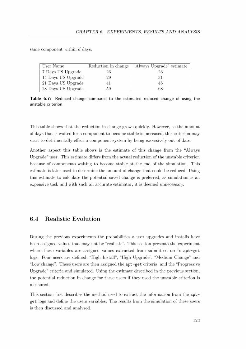
CHAPTER 6. EXPERIMENTS, RESULTS AND ANALYSIS
same component within d days.
User Name Reduction in change “Always Upgrade” estimate
7 Days US Upgrade 23 2314 Days US Upgrade 29 3121 Days US Upgrade 41 4628 Days US Upgrade 59 68
Table 6.7: Reduced change compared to the estimated reduced change of using theunstable criterion.
This table shows that the reduction in change grows quickly. However, as the amount
of days that is waited for a component to become stable is increased, this criterion may
start to detrimentally effect a component system by being excessively out-of-date.
Another aspect this table shows is the estimate of this change from the “Always
Upgrade” user. This estimate differs from the actual reduction of the unstable criterion
because of components waiting to become stable at the end of the simulation. This
estimate is later used to determine the amount of change that could be reduced. Using
this estimate to calculate the potential saved change is preferred, as simulation is an
expensive task and with such an accurate estimator, it is deemed unnecessary.
6.4 Realistic Evolution
During the previous experiments the probabilities a user upgrades and installs have
been assigned values that may not be “realistic”. This section presents the experiment
where these variables are assigned values extracted from submitted user’s apt-get
logs. Four users are defined, “High Install”, “High Upgrade”, “Medium Change” and
“Low change”. These users are then assigned the apt-get criteria, and the “Progressive
Upgrade” criteria and simulated. Using the estimate described in the previous section,
the potential reduction in change for these users if they used the unstable criterion is
measured.
This section first describes the method used to extract the information from the apt-
get logs and define the users variables. The results from the simulation of these users
is then discussed and analysed.
123
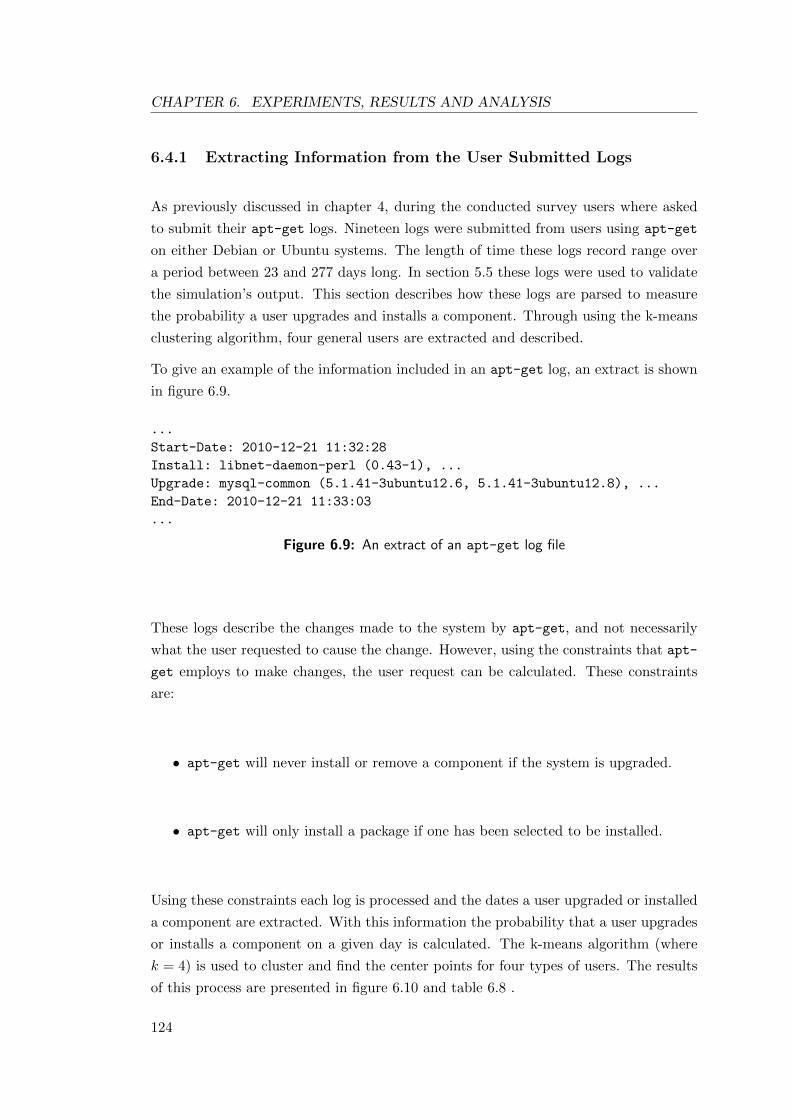
CHAPTER 6. EXPERIMENTS, RESULTS AND ANALYSIS
6.4.1 Extracting Information from the User Submitted Logs
As previously discussed in chapter 4, during the conducted survey users where asked
to submit their apt-get logs. Nineteen logs were submitted from users using apt-get
on either Debian or Ubuntu systems. The length of time these logs record range over
a period between 23 and 277 days long. In section 5.5 these logs were used to validate
the simulation’s output. This section describes how these logs are parsed to measure
the probability a user upgrades and installs a component. Through using the k-means
clustering algorithm, four general users are extracted and described.
To give an example of the information included in an apt-get log, an extract is shown
in figure 6.9.
...
Start-Date: 2010-12-21 11:32:28
Install: libnet-daemon-perl (0.43-1), ...
Upgrade: mysql-common (5.1.41-3ubuntu12.6, 5.1.41-3ubuntu12.8), ...
End-Date: 2010-12-21 11:33:03
...
Figure 6.9: An extract of an apt-get log file
These logs describe the changes made to the system by apt-get, and not necessarily
what the user requested to cause the change. However, using the constraints that apt-
get employs to make changes, the user request can be calculated. These constraints
are:
• apt-get will never install or remove a component if the system is upgraded.
• apt-get will only install a package if one has been selected to be installed.
Using these constraints each log is processed and the dates a user upgraded or installed
a component are extracted. With this information the probability that a user upgrades
or installs a component on a given day is calculated. The k-means algorithm (where
k = 4) is used to cluster and find the center points for four types of users. The results
of this process are presented in figure 6.10 and table 6.8 .
124
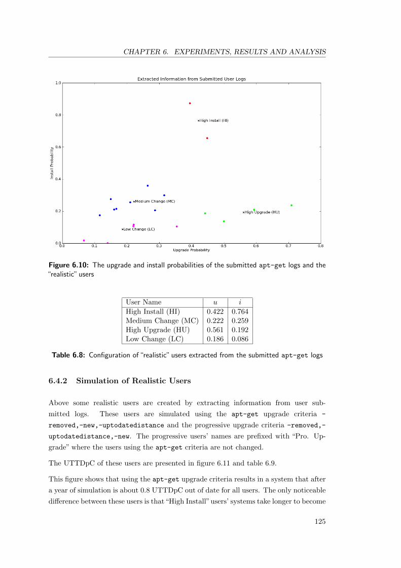
CHAPTER 6. EXPERIMENTS, RESULTS AND ANALYSIS
Figure 6.10: The upgrade and install probabilities of the submitted apt-get logs and the“realistic” users
User Name u i
High Install (HI) 0.422 0.764Medium Change (MC) 0.222 0.259High Upgrade (HU) 0.561 0.192Low Change (LC) 0.186 0.086
Table 6.8: Configuration of “realistic” users extracted from the submitted apt-get logs
6.4.2 Simulation of Realistic Users
Above some realistic users are created by extracting information from user sub-
mitted logs. These users are simulated using the apt-get upgrade criteria -
removed,-new,-uptodatedistance and the progressive upgrade criteria -removed,-
uptodatedistance,-new. The progressive users’ names are prefixed with “Pro. Up-
grade” where the users using the apt-get criteria are not changed.
The UTTDpC of these users are presented in figure 6.11 and table 6.9.
This figure shows that using the apt-get upgrade criteria results in a system that after
a year of simulation is about 0.8 UTTDpC out of date for all users. The only noticeable
difference between these users is that“High Install”users’ systems take longer to become
125
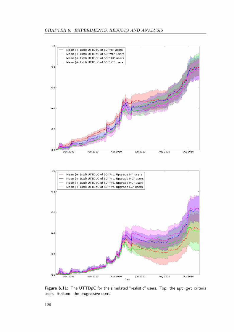
CHAPTER 6. EXPERIMENTS, RESULTS AND ANALYSIS
Figure 6.11: The UTTDpC for the simulated “realistic” users. Top: the apt-get criteriausers. Bottom: the progressive users.
126
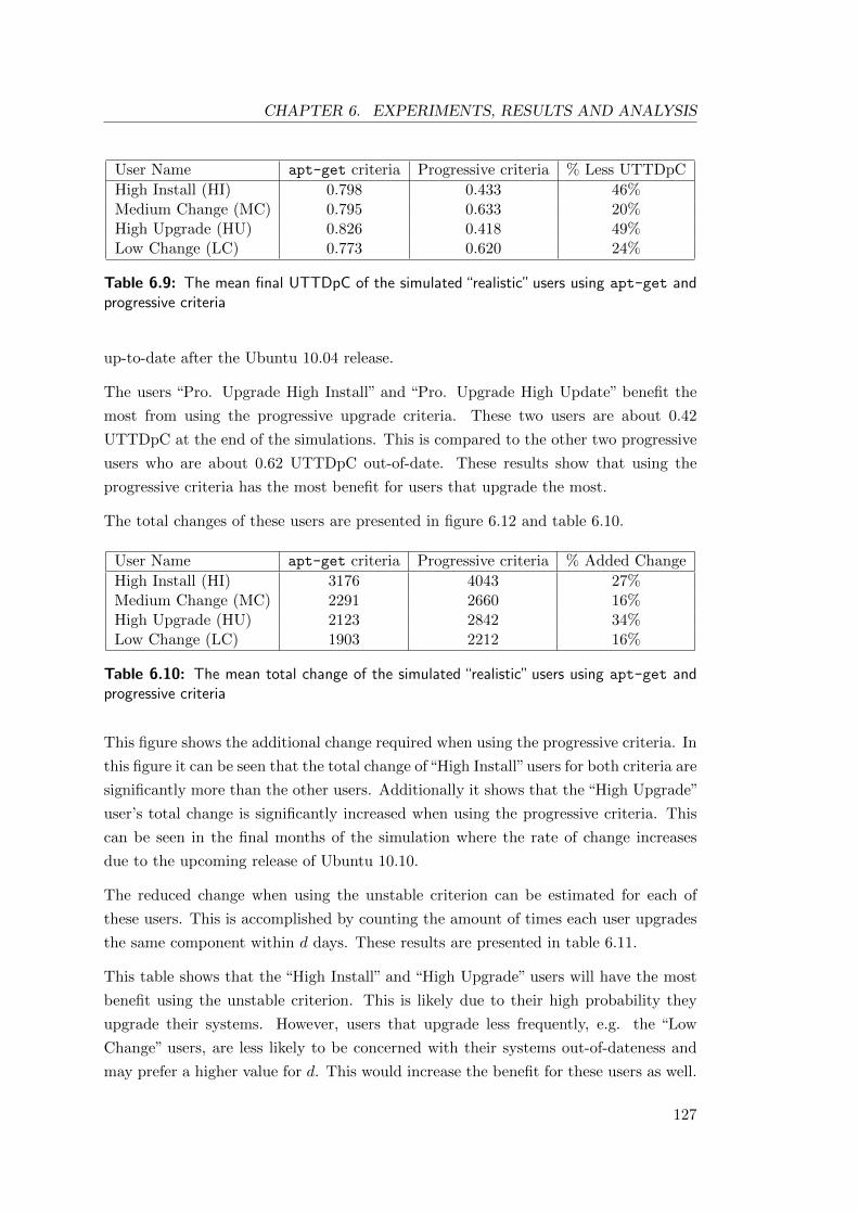
CHAPTER 6. EXPERIMENTS, RESULTS AND ANALYSIS
User Name apt-get criteria Progressive criteria % Less UTTDpC
High Install (HI) 0.798 0.433 46%Medium Change (MC) 0.795 0.633 20%High Upgrade (HU) 0.826 0.418 49%Low Change (LC) 0.773 0.620 24%
Table 6.9: The mean final UTTDpC of the simulated “realistic” users using apt-get andprogressive criteria
up-to-date after the Ubuntu 10.04 release.
The users “Pro. Upgrade High Install” and “Pro. Upgrade High Update” benefit the
most from using the progressive upgrade criteria. These two users are about 0.42
UTTDpC at the end of the simulations. This is compared to the other two progressive
users who are about 0.62 UTTDpC out-of-date. These results show that using the
progressive criteria has the most benefit for users that upgrade the most.
The total changes of these users are presented in figure 6.12 and table 6.10.
User Name apt-get criteria Progressive criteria % Added Change
High Install (HI) 3176 4043 27%Medium Change (MC) 2291 2660 16%High Upgrade (HU) 2123 2842 34%Low Change (LC) 1903 2212 16%
Table 6.10: The mean total change of the simulated “realistic” users using apt-get andprogressive criteria
This figure shows the additional change required when using the progressive criteria. In
this figure it can be seen that the total change of“High Install”users for both criteria are
significantly more than the other users. Additionally it shows that the “High Upgrade”
user’s total change is significantly increased when using the progressive criteria. This
can be seen in the final months of the simulation where the rate of change increases
due to the upcoming release of Ubuntu 10.10.
The reduced change when using the unstable criterion can be estimated for each of
these users. This is accomplished by counting the amount of times each user upgrades
the same component within d days. These results are presented in table 6.11.
This table shows that the “High Install” and “High Upgrade” users will have the most
benefit using the unstable criterion. This is likely due to their high probability they
upgrade their systems. However, users that upgrade less frequently, e.g. the “Low
Change” users, are less likely to be concerned with their systems out-of-dateness and
may prefer a higher value for d. This would increase the benefit for these users as well.
127
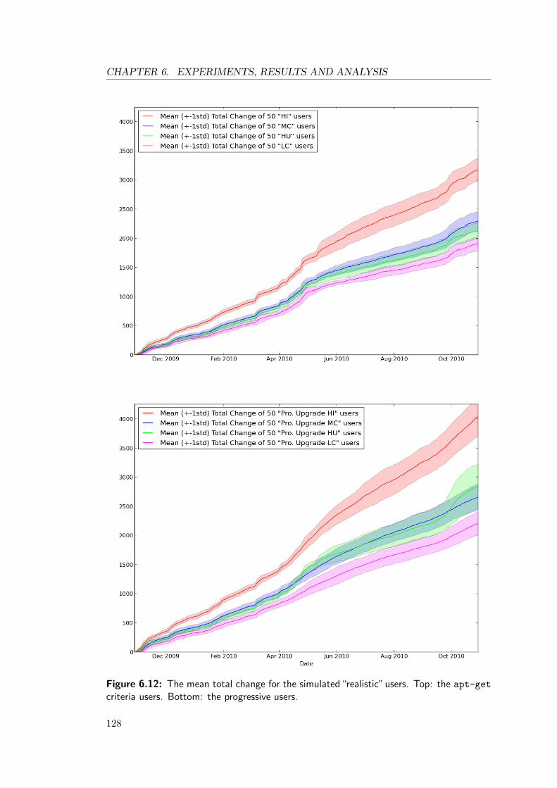
CHAPTER 6. EXPERIMENTS, RESULTS AND ANALYSIS
Figure 6.12: The mean total change for the simulated“realistic”users. Top: the apt-get
criteria users. Bottom: the progressive users.
128
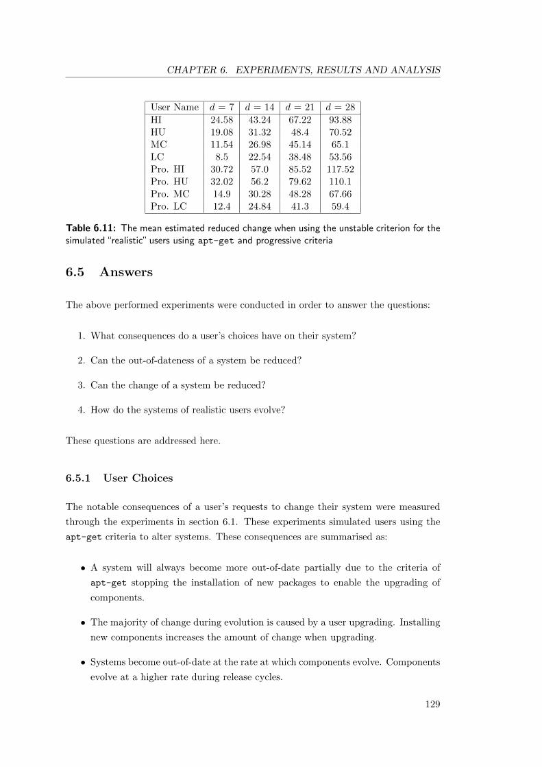
CHAPTER 6. EXPERIMENTS, RESULTS AND ANALYSIS
User Name d = 7 d = 14 d = 21 d = 28
HI 24.58 43.24 67.22 93.88HU 19.08 31.32 48.4 70.52MC 11.54 26.98 45.14 65.1LC 8.5 22.54 38.48 53.56Pro. HI 30.72 57.0 85.52 117.52Pro. HU 32.02 56.2 79.62 110.1Pro. MC 14.9 30.28 48.28 67.66Pro. LC 12.4 24.84 41.3 59.4
Table 6.11: The mean estimated reduced change when using the unstable criterion for thesimulated “realistic” users using apt-get and progressive criteria
6.5 Answers
The above performed experiments were conducted in order to answer the questions:
1. What consequences do a user’s choices have on their system?
2. Can the out-of-dateness of a system be reduced?
3. Can the change of a system be reduced?
4. How do the systems of realistic users evolve?
These questions are addressed here.
6.5.1 User Choices
The notable consequences of a user’s requests to change their system were measured
through the experiments in section 6.1. These experiments simulated users using the
apt-get criteria to alter systems. These consequences are summarised as:
• A system will always become more out-of-date partially due to the criteria of
apt-get stopping the installation of new packages to enable the upgrading of
components.
• The majority of change during evolution is caused by a user upgrading. Installing
new components increases the amount of change when upgrading.
• Systems become out-of-date at the rate at which components evolve. Components
evolve at a higher rate during release cycles.
129
CHAPTER 6. EXPERIMENTS, RESULTS AND ANALYSIS
• Reuse decreases the rate of change during CSE. This is due to the two effects;
reuse decreases the installation rate of components and this decreases the amount
of components necessary to be upgraded.
• There were two types of failures observed to occur:
– Hard failures: where the constraints of a request could not be satisfied.
These occurred 0.12% during the simulation.
– Soft failures: where the constraints were satisfied, though the returned
solution was possibly not optimal. These occurred in 3% of the requests,
though only 1% of these were determined to be detrimental to the system.
Such detrimental soft failures occur more frequently during release cycles
when components are evolving at a higher rate.
• Increasing the frequency of upgrading has depreciating returns on reducing a
systems out-of-dateness. It may also increase change due to components being
repeatedly upgraded if they quickly release multiple versions.
6.5.2 Reduce Out-of-dateness
As noted above, a system becomes out-of-date partially due to the apt-get criteria not
allowing new components to be installed. To remove this restriction the order of the
apt-get criteria was altered to the “progressive” criteria. Using this criteria to upgrade
a system every day was shown to decrease the out-of-dateness by 24% at the cost of
increasing change by 21%. This additional change was due to the new components
being installed and upgraded during the simulation.
6.5.3 Reduce Change
Some of the change caused when upgrading a system was due to rapidly released
components being repeatedly upgraded. For a user that upgrades every day, there
were 23 occasions were a component being upgraded twice within a week. This is
unnecessary change that introduces risk into a system. The unstable criterion was
defined to reduce this change by waiting for a component to become stable over a
period of days. The cost of using the unstable criterion was the system remains out-
of-date by the number of days waited for components to become stable. However,
through using the unstable criterion waiting a week for components to become stable
all 23 instances of this unnecessary change were removed.
130
CHAPTER 6. EXPERIMENTS, RESULTS AND ANALYSIS
6.5.4 Real Users
To simulate realistic users the probability a user upgrades and installs were extracted
from user’s submitted logs. Using the k-means algorithm four stereotypes of user were
created; ‘High Install”, “High Upgrade”, “Medium Change” and “Low change”. These
users were simulated using the apt-get criteria and the progressive criteria, and the
lowered change from using the unstable criterion was estimated. This has shown that
the greatest benefits for using the progressive criteria and the unstable criterion is for
the “High Install” and “High Upgrade” users. This is due to their higher frequency they
upgrade their systems.
6.6 Summary
This chapter presented a series of experiments that simulated various users to study
CSE. These experiments explored the consequences of users changing their systems,
and the novel proposed progressive and unstable criteria. The next chapter describes
the conclusions, the related work, and the potential future research of CSE.
131
CHAPTER 6. EXPERIMENTS, RESULTS AND ANALYSIS
132
Chapter 7
Conclusion
This research has investigated the evolution of component systems using a developed
simulation. To build this simulation, first the background of software evolution,
component-based software engineering and component systems were explored (chapter
2). The models CoSyE (chapter 3) and SimUser (chapter 4) were then developed to
describe a component system evolving through repetitive change and the user that
requests the changes. GJSolver (chapter 5) was then created to calculate the exact
changes made to a system during evolution. The verification and validation of these
artifacts were discussed, in accordance with the methodology (Law, 2005).
Experiments were defined that use these artifacts to simulate the evolution of many
different systems. The primary focus of these experiments was to measure and reduce
the out-of-dateness and changes made to the systems during evolution. The experiments
have provided empirical evidence:
• Upgrading a system causes the majority of change and installing new components
only adds to this change by increasing the number of components to be upgraded.
• Upgrading frequently (i.e. once a day) is unnecessary as it has little impact on
the out-of-dateness of systems. However, during periods where new component
versions are released quickly, e.g. during Ubuntu releases, it is important to
upgrade frequently.
• Regular updates cannot ensure that a component system stays up-to-date. This is
in part due to the criteria used by apt-get that restricts adding new components
when upgrading.
• Frequently upgrading a system may cause additional change when many versions
of a component are released quickly, forcing it to be upgraded multiple times.
133
CHAPTER 7. CONCLUSION
This research also provides empirical evidence and quantitative measurements of the
benefit of reuse, especially during CSE. The main benefit during CSE is the reduced
change due to lowering the amount of components to be installed, that in turn lowers
the amount of components that are upgraded. Reuse was estimated to save 650 changes
on a system during the year.
To reduce the out-of-dateness of systems during evolution, the progressive criteria was
proposed. This criteria allows new components to be installed to enable the upgrading
of components. This alteration was shown to be most effective for users that upgrade
frequently. It was shown to decrease the out-of-dateness of a system by as much as 49%
at the cost of increasing change by 34%. For users that prefer up-to-date systems, this
trade-off might be favourable for their system.
To reduce the change made to a system during CSE the unstable criterion was proposed.
This criterion waits for a period of days for a component to cease releasing newer version
and become stable. By using this criterion and waiting a week for a component to
become stable before upgrading it, it was estimated to save some types of users more
than 30 changes over a year. These changes could introduce bugs into the system and
are seen as unnecessary. Using this criterion comes at the cost of the system always
being out-of-date by the number of days that are waited for components to become
stable. For users that prefer to reduce change to their systems, this may be a tolerable
trade-off.
The remainder of this chapter will examine the proposed thesis in chapter 1, the
potential future research, and provide a closing remark.
7.1 Thesis Validation
This research started with the thesis:
It is possible to reduce the negative effects of component system evolution by
altering the mechanisms by which systems are changed.
The steps taken to validate this thesis were:
• To develop a reproducible and controllable environment in which to measure the
effects of CSE.
• To use this environment to study how systems evolve.
134

CHAPTER 7. CONCLUSION
• To alter the mechanisms by which systems are changed and study their impact
on CSE.
• To demonstrate a reduction on change and out-of-dateness using such alterations.
To address these steps:
• A simulation was developed.
• It was used to study CSE through simulating the evolution of many Ubuntu
systems.
• The novel unstable criterion and progressive criteria were proposed and their
impacts on CSE studied.
• The unstable criterion and progressive criteria were then simulated to approx-
imate the evolution of real component systems and they were demonstrated to
reduce change and out-of-dateness.
It is therefore possible to conclude that the thesis is supported.
7.2 Future Research
The largest area of future research is in the simulation of additional systems, such
as Eclipse, so they can be studied as they evolve. Through such simulation the
conclusions of this research can be shown to be either invariant between component
systems or to be Ubuntu-specific. The core hurdle of accomplishing this is that much
of the collected information in this study does not exist for other component models.
Component models like Eclipse do not have their history archived as precisely as
Ubuntu. Information, like the Ubuntu repository, does not exist or does not contain
the detailed information for other component models. Resources of information are
available, but can be incomplete. For example, the Usage Data Collector1 for the
Eclipse project (similar to the Ubuntu Popcon) collected information on popular Eclipse
components. However, this project was shut down as it was deemed not to have a
significant return on investment.
Another area of research involves altering and extending the CoSyE and SimUser
models to more precisely describe CSE. An aspect of CSE that is not included in
CoSyE is that a component system may only view a certain subset of components that
1http://www.eclipse.org/epp/usagedata/faq.php
135
CHAPTER 7. CONCLUSION
exist. This is described in section 4.4 as the view Ubuntu has of its repository. The
SimUser has many aspects that could be added to make the simulated users closer to
reality. Constraints such as only upgrading during the work week, or additional types
of request like removal of components that are no longer required, could create more
valid simulations.
The development of criteria that use other properties of components, could be used to
more accurately represent the user’s preferences. Such properties could be collected
from additional sources, e.g. component meta-data, component contracts (Watkins
et al., 1999), repositories (Guo and Luqi, 2000), composition testing (Li et al., 2008).
These could be used to create criteria that optimise for size, reliability, licence, even
validity. Such criteria could be simulated and their effect, positive or negative, could
be measured using the simulation developed in this research.
The part of the simulation that has the most room for improvement is the selection
of the requests made by the user. This is when they select to upgrade, when they
select to install, and what components they select to install. By studying real users
changing their systems, either through collecting more apt-get logs or through direct
observation, a more valid simulation could be created.
Comparing the results from the simulations to the evolution of real systems would be
able to validate the conclusions drawn from the simulation. This could be accomplished
using the MPM solver (Abate and DiCosmo, 2011) from Mancoosi. This solver has
already been proposed for the modification of real systems. Through modification or
extension of MPM, the proposed criteria could be used to evolve real Ubuntu systems.
Such a study would require significant resources, but its results and conclusions would
be worthwhile as they could provide a direct benefit to a very large number of users.
7.3 Closing Remark
This research has given an understanding of how component systems evolve and can
be used to provide users and developers with insights into the effects of their choices.
Additionally, this research has proposed two novel ways to reduce negative effects during
CSE and the tools in with which to measure the effectiveness of these techniques. This
research, therefore, has the potential of impacting the millions of Ubuntu and Eclipse
systems that are currently evolving.
136
Appendix A
CUDF* Parsing to CoSyE
Instance
In this section, the parsing of a CUDF* document (presented in section 3.1) to a CoSyE
instance is described.
The package stanzas in the document define the sets of components Ct1 , . . . , Ctn ,
the initial component system αt0 , and the sets of system constraints ωt1 , . . . , ωtn .
The preamble stanza describes the time t0, the request stanzas define a series of
times t1, . . . , tn, sets of user requests δt1 , . . . , δtn , and the evolution preference orders
≺αt0, . . . ,≺αtn−1
.
A.1 CUDF* BNF Grammar
The CUDF* language is described in the EBNF grammar presented in figure A.1. This
is an extension of the CUDF EBNF grammar given by Mancoosi1 combined with the
MOF EBNF grammar. The notable differences between CUDF and CUDF* is that
there can be multiple requests, where each request defines a time and a MOF criteria.
Other differences are that the premable defines a time value, and each component must
also define a time value.
1http://www.mancoosi.org/cudf/ebnf/ visited 26/3/2012
137
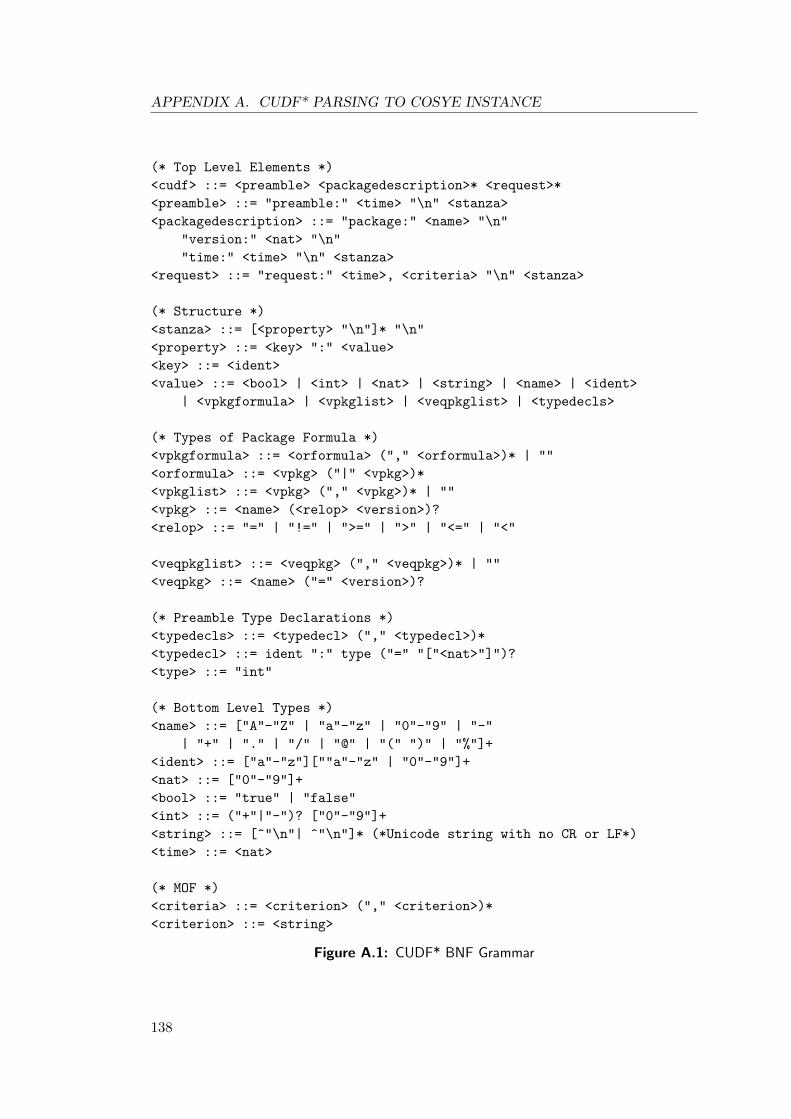
APPENDIX A. CUDF* PARSING TO COSYE INSTANCE
(* Top Level Elements *)
<cudf> ::= <preamble> <packagedescription>* <request>*
<preamble> ::= "preamble:" <time> "\n" <stanza>
<packagedescription> ::= "package:" <name> "\n"
"version:" <nat> "\n"
"time:" <time> "\n" <stanza>
<request> ::= "request:" <time>, <criteria> "\n" <stanza>
(* Structure *)
<stanza> ::= [<property> "\n"]* "\n"
<property> ::= <key> ":" <value>
<key> ::= <ident>
<value> ::= <bool> | <int> | <nat> | <string> | <name> | <ident>
| <vpkgformula> | <vpkglist> | <veqpkglist> | <typedecls>
(* Types of Package Formula *)
<vpkgformula> ::= <orformula> ("," <orformula>)* | ""
<orformula> ::= <vpkg> ("|" <vpkg>)*
<vpkglist> ::= <vpkg> ("," <vpkg>)* | ""
<vpkg> ::= <name> (<relop> <version>)?
<relop> ::= "=" | "!=" | ">=" | ">" | "<=" | "<"
<veqpkglist> ::= <veqpkg> ("," <veqpkg>)* | ""
<veqpkg> ::= <name> ("=" <version>)?
(* Preamble Type Declarations *)
<typedecls> ::= <typedecl> ("," <typedecl>)*
<typedecl> ::= ident ":" type ("=" "["<nat>"]")?
<type> ::= "int"
(* Bottom Level Types *)
<name> ::= ["A"-"Z" | "a"-"z" | "0"-"9" | "-"
| "+" | "." | "/" | "@" | "(" ")" | "%"]+
<ident> ::= ["a"-"z"][""a"-"z" | "0"-"9"]+
<nat> ::= ["0"-"9"]+
<bool> ::= "true" | "false"
<int> ::= ("+"|"-")? ["0"-"9"]+
<string> ::= [^"\n"| ^"\n"]* (*Unicode string with no CR or LF*)
<time> ::= <nat>
(* MOF *)
<criteria> ::= <criterion> ("," <criterion>)*
<criterion> ::= <string>
Figure A.1: CUDF* BNF Grammar
138

APPENDIX A. CUDF* PARSING TO COSYE INSTANCE
A.2 Additional Stanza Constraints
In figure A.1, a CUDF* document is described as a preamble, a list of package
descriptions, and a list of requests. The preamble is a stanza started with the text
preamble:. A package description is a stanza started with the text package: followed
by a package name, a package version, and a time. A request is a stanza started with
the text request:, followed by a time and a MOF criteria string.
This grammar does not list all the constraints for each stanza, and each property. For
example, the property with key installed can only be in a package description, and
can only have a <bool> value. Each stanza type (preamble, package description or
request) can consist of different properties, where each properties value can be of a
different type. In tables A.1, A.2 and A.3, the allowed properties for the preamble, a
package description, and the request are described respectively.
Property Name Value Type Default Value
property <typedecl> ""
Table A.1: CUDF* Preamble properties
Property Name Value Type Default Value
depends <vpkgformula> ""
conflicts <vpkglist> ""
provides <veqpkglist> ""
installed <bool> "false"
keep <ident> either "version", "package", or "none" "none"
Table A.2: CUDF* Package Description properties
Property Name Value Type Default Value
install <vpkglist> ""
remove <vpkglist> ""
upgrade <vpkglist> | "*" ""
Table A.3: CUDF* Request properties
In addition to the properties allowed in the package description, as presented in table
A.2, extra properties can be defined in the preamble’s property property. This is
described in section 3.2.1.3, and restricted to only defining new <int> typed properties.
139
APPENDIX A. CUDF* PARSING TO COSYE INSTANCE
A.3 Parsing
How a CUDF* represented and parsed to create the CoSyE instance is described in
this section.
Definition 41 A CUDF* document is a tuple containing a preamble stanza
(preamble), a set of package description stanzas (PD), and set of request stanzas
(REQUESTS), i.e. 〈premable, PD,REQUESTS〉.
Each stanza can be seen as a function:
Definition 42 A stanza is a function that takes a key key, and returns a value value,
s(key) =value.
This function is abbreviated to use the infix notation ., i.e. s.key=value. For a
package description stanza pd, pd.name returns the <name> value, pd.version returns
the <nat> value, and pd.time returns the time value. For a request stanza r, r.time
returns the time value, and r.criteria returns the criteria value. For the preamble
stanza premable, premable.time returns the time value.
The set of times T is the set of natural numbers N, totally ordered under ≤. The set
of names N is the set of strings that match the regular expressions of <name> in figure
A.1. The set of versions V is the set of natural numbers N, totally ordered under ≤.
The first definition is to define the series of times.
Definition 43 Given a CUDF* document 〈premable, PD,REQUESTS〉, t0 is de-
fined as premable.time, and t1, . . . , tn are defined as r1.time, . . . , rn.time where
REQUESTS = r1, . . . , rn.
A.4 Components
The sets of components Ct0 , . . . , Ctn , and component system αt0 are defined given a
CUDF* document.
Definition 44 The function pd2c is defined to take a package description stanza pd,
and return a component, pd2c(pd) = 〈pd.name, pd.version 〉.
The infix notation . can also be used to abbreviate component properties, e.g. for a
package description pd, and component c = vpd2c(pd), pd.name = c.name.
140
APPENDIX A. CUDF* PARSING TO COSYE INSTANCE
Definition 45 Given a CUDF* document 〈premable, PD,REQUESTS〉, a set of
components Ct is defined as the set of package descriptions mapped using the function
pd2c, whose time value is less than or equal to t, i.e. Ct = pd2c(pd) | pd ∈PD and pd.time≤ t
Ct is then a “slice” of the components that existed at time t. The sets of components
Ct0 , . . . , Ctn are defined as slices of the set of components given the times t0, . . . , tn.
Definition 46 Given a CUDF* document 〈premable, PD,REQUESTS〉, and set of
components Ct0, the initial component system αt0 is the set of components in Ct0 whose
installed property equals true, i.e. αt0 = c | c ∈ Ct0 and c.installed = "true"
A.5 Features
CUDF* specifies an additional aspect to system constraints, that of a feature (this can
also be described as a service, or a virtual package). Each component can provide
a many features, more over, a component can provide many versions of a feature.
Therefore, a component provides a set of features, where each feature has a name, and
a set of versions.
Definition 47 A feature f is a pair consisting of a name n ∈ N and a set of versions
V ⊆ V , i.e. f = 〈n, V 〉
The features provided by a component are defined in the property with key provides,
which is of the type <veqpkglist>. This type is a list of <veqpkg>, either of the form
<name> or <name> "=" <version>.
• <name> := (<name>,V)
• <name> = <version> := (<fname>, <version>)
That is, a <veqpkg> which does not define a version, is defined as a feature that provides
all versions. A <veqpkg> the defines a version, is defined as a feature that provides a
singleton set of that version.
Definition 48 The function providedFeatures is defined to take a component c, and
return the set of features that component provides, providedFeatures(c) = the set of
features mapped from the c.provides value.
141
APPENDIX A. CUDF* PARSING TO COSYE INSTANCE
For example, a component a is defined such that a.provides = "n = 10, m"; the
function providedFeatures(a) returns the set of features ("n", 10), ("m",V).
A.6 Package formula
A package formula, of type <vpkg>, is a query for a set of components from a CUDF*
document. This formula is the mechanism that defines all constraints and requests in
the CUDF specification.
Each <vpkg> is of the form “<name>” or “<name> <relop> <version>”.
Definition 49 A package formula pf is a triple, name n, version v, and relation r,
pf = 〈n, v, r〉.
The syntax of <relop> is parsed to a mathematical relation with the function relop:
relop = "=" → =, "!=" →6=, ">=" → ≥, ">" → >, "<=" → ≤, "<" → <.
• <name> := 〈<name>, 0, >〉
• <name> <relop> <version> := 〈<name>, <version>, relop(<relop>)〉
That is, a <vpkg> that does not define a relation or version, is defined as a package
formula that is greater than zero.
Definition 50 A component c = 〈n, v〉 satisfies a package formula 〈m,w, r〉 iff
(n = m and v r w), or (∃(o, V ) ∈ providedFeatures(c) where o = n and ∃x ∈ V
such that v r x).
That is, a component satisfies a package formula if it has the same name, and its version
relates to the package formula version; or the component provides a feature with the
same name that contains a version that relates to package formula version.
Definition 51 Given a set of components Cti, the function packagesThatSatisfy
takes a package formula pf and returns all components in Cti that satisfy it, i.e.
packagesThatSatisfy(pf) = c | c ∈ Cti and c satisfies pf
142
APPENDIX A. CUDF* PARSING TO COSYE INSTANCE
A.6.1 Sets of Package Formula
The elements <orformula> and <vpkglist> are both lists of <vpkg>’s. The element
<vpkgformula> is a list of <orformula>’s, therefore is a list of lists of <vpkg>’s.
The mapping of these elements is trivial:
• <orformula> := a set of package formula.
• <vpkglist> := a set of package formula.
• <vpkgformula> := a set of sets of package formula.
Definition 52 Given a set of components Cti, the function allPackagesThatSatisfy
takes a set of package formula pkgflist and returns all components in Cti that
satisfy any package formula in the set, i.e. allPackagesThatSatisfy(pkgflist) =⋃pf∈pkgflist
packagesThatSatisfy(pf)
A.7 System Constraints
Given a CUDF* document, there are three sets of constraints that make up a set of
system constraints ωti , each containing a different constraint type:
• keep constraints ωkeeptiare extracted from the values of keep properties of
components in αti−1 .
• dependency constraints ωdeptiare extracted from the values of depends properties
of components in Cti .
• conflict constraints ωconti are extracted from the conflicts properties of
components in Cti .
A set of system constraints ωti is the union of these, ωti = ωkeepti∪ωdepti
∪ωconti . Therefore,
the sets of system constraints ωt1 , . . . , ωtn can be defined from a CUDF* document.
A.7.1 Keep Constraints
Given a CUDF* document, a set of keep constraints is ωkeepti. These constraints are
extracted from the property with the key keep in the components in αti−1 .
The values of the property with key keep can be either none, version, or package. If
the value is none, then no constraints are generated.
143
APPENDIX A. CUDF* PARSING TO COSYE INSTANCE
Definition 53 The function keep takes a component c, and returns a set of keep
constraints, such that
• if c.keep equals "none": keep(c) = ∅
• if c.keep equals "version": keep(c) = c
• if c.keep equals "package": keep(c) = a1 ∨ . . . ∨ an where a1, . . . , an = b |b ∈ Cti and b.name = c.name
That is, the function keep takes a component c and to return a set of keep constraints
where
• if the value of c.keep equals "none" then no constraints are required.
• if the value of c.keep equals "version", the set of constraints ensures that the
component c will be kept in the system.
• if the value of c.keep equals "package", the constraint ensures that at least one
component with the same name as c will be kept in the system.
The set of all keep constraints can be defined as:
Definition 54 Given the component system αti−1, ωkeepti=
⋃c∈αti−1
keep(c).
A.7.2 Dependency Constraint
Given a CUDF* document, the set of dependency constraints is ωdepti. These constraints
are extracted from the property depends in the components in the set Cti . The value
of the property with key depends is a <vpkgformula> which is mapped to a set of sets
of package formula.
Definition 55 Given a CUDF* document, the function dependsOn takes a component
a and a set of package formula pkgflist and returns a set with a single dependency
constraint, such that dependsOn(a, pkgflist) returns a → c1 ∨ . . . cn where
c1, . . . , cn = allPackagesThatSatisfy(pkgflist).
That is, dependsOn(a, pkgflist) creates the dependency constraint where a depends
on the disjunction of the union of all components that satisfy a package formula set.
144
APPENDIX A. CUDF* PARSING TO COSYE INSTANCE
Definition 56 Given a CUDF* document, the function depends takes a component
a, and returns a set of dependency constraints, such that depends(a) returns⋃pkgflst∈listpkgflist
dependsOn(a, pkgflst), where listpkgflist is mapped from the value
a.depends.
That is, depends returns the set of all dependency constraints for a component from
its depends property.
The set of all dependency constraints can be defined as:
Definition 57 Given the set of components Cti, ωdepti
=⋃
a∈Cti
depends(a).
A.7.3 Conflict Constraint
Given a CUDF* document, the set of conflict constraints is ωconti . These constraints are
extracted from the property conflicts in the components in the set Cti . The value of
the property with key conflicts is a <vpkglist> mapped to a set of package formula.
Definition 58 Given a CUDF* document, the function conflicts takes a component
a, and returns a set of conflict constraints, such that conflicts(a) returns a → ¬c |c ∈ allPackagesThatSatisfy(pkgflist) and c 6= a, where pkgflist is mapped from
the value a.conflicts.
That is, the component a conflicts with any component that satisfies a package formula
in its conflict property, with the exception is that a component cannot conflict with
itself.
The set of all conflict constraints can be defined as:
Definition 59 Given the set of components Cti, ωconti =⋃
a∈Cti
conflicts(a).
A.8 Request
Given a CUDF* document, there are three sets of constraints that make up a set of
request constraints δti , each containing a different user request type:
• the set of installation request constraints δinsti is extracted from value r.install
where r is the request stanza such that r.time = ti.
145
APPENDIX A. CUDF* PARSING TO COSYE INSTANCE
• the set of remove request constraints δremti is extracted from the value r.remove
where r is the request stanza such that r.time = ti.
• the set of upgrade constraints δupgtiis extracted from the value r.upgrade where
r is the request stanza such that r.time = ti.
A set of user request constraints δti is the union of these, δti = δinsti ∪ δremti ∪ δupgti
.
Therefore, the sets of requests δt1 , . . . , δtn can be defined from a CUDF* document.
A.8.1 Install
Given a CUDF* document, δinsti is extracted from value r.install where r is the request
stanza such that r.time = ti. The value r.install is of type <vpkglist> which can
be mapped to a set of package formula.
Definition 60 Given a CUDF* document, the function install takes a package formula
pf and returns a set containing one install request constraint, such that install(pf) =
a1 ∨ . . . ∨ an where a1, . . . , an = packagesThatSatisfy(pf).
Definition 61 Given a CUDF* document, a set of install request constraints δinsti =⋃pf∈pkgflist
install(pf), where pkgflist is the set of package formula mapped from value
r.install where r is the request stanza such that r.time = ti.
A.8.2 Remove
Given a CUDF* document, δremti is extracted from value r.remove where r is the request
stanza such that r.time = ti. The value of r.remove is of type <vpkglist> which can
be mapped to a set of package formula.
Definition 62 Given a CUDF* document, a set of remove request constraints δremti
equals ¬a | a ∈ allPackagesThatSatisfy(pkgflist), where pkgflist is the set of
package formula mapped from value r.remove where r is the request stanza such that
r.time = ti.
A.8.3 Upgrade
Given a CUDF* document, the set of upgrade requests δupgtiis extracted from the value
request.upgrade. If the value r.upgrade is of type <vpkglist>, it can be mapped to
146
APPENDIX A. CUDF* PARSING TO COSYE INSTANCE
a set of package formula. If the value of r.upgrade is equal to *, it can be mapped to
a set of package formula where 〈n, 0, >〉 | 〈n, v〉 ∈ αti−1. That is, if the upgrade is
requested to upgrade *, then the request is to upgrade all packages currently installed.
Given a package formula, 〈n, v, op〉, an upgrade request contains two constraints:
1. only one component with the name n can be in the evolved system, this is
constraint type 5.
2. the component with name n should be have a greater than, or equal to, version
than the component with name n with the greatest version in αti−1 .
The first upgrade constraint:
Definition 63 Given a CUDF* document, the function upgrade1 takes a component
name n and returns an upgrade request constraint, upgrade1(n) = a1 + . . . + ai = 1
where a1, . . . , ai = packagesThatSatisfy(〈n, 0, >〉).
That is, upgrade1 returns the constraint that ensures exactly one version of a component
with name n will be in the evolved system.
The utility function maxversion is required:
Definition 64 Given a CUDF* document with component system αti−1, the function
maxversion takes a name n and returns the highest version of a component in αti−1
with name n, maxversion(n) = v | 〈n, v〉 ∈ αti−1 and there is no other component
〈n, v′〉 ∈ αti−1 where v < v′.
The second upgrade constraint:
Definition 65 Given a CUDF* document, the function upgrade2 takes a package
formula and returns an upgrade constraint, upgrade2(n) = a1 + . . . + ai = 1 where
a1, . . . , ai = packagesThatSatisfy(〈n,maxversion(n),≥〉).
That is, upgrade2 returns the constraint that the version of the component with name
n in the evolved system, must be greater than the maxversion can be in the evolved
system.
Definition 66 Given a CUDF* document, a set of upgrade request constraints δupgti
equals⋃
〈n,v,op〉∈pkgflistupgrade1(n), upgrade2(n), where pkgflist is the set of package
formula mapped from value r.upgrade where r is the request stanza such that r.time
= ti.
147
APPENDIX A. CUDF* PARSING TO COSYE INSTANCE
A.9 Criteria
Given a CUDF* document, an evolutionary preference order ≺αti−1is extracted from
the value r.criteria where r is the request stanza such that r.time = ti. The value
r.criteria is a list of criterion separated by the delimiter “,” that can be mapped
to a tuple of strings 〈criterion1, . . . , criterionn〉.
Definition 67 A partial function critmap is defined such that it takes a string
criterionj and returns a criterion (from CoSyE) 〈rankjα,≤j〉, i.e. critmap(criterionj) =
〈rankjα,≤j〉.
A single lexicographic criterion 〈rankLα ,≤L〉 is defined using ⊕ as critmap(criterion1)⊕. . .⊕ critmap(criterionn). 〈rankLα ,≤L〉 is used to create the evolution optimality order
≺αti−1as described in definition 17.
This can be used to define the optimality orders ≺αt0, . . . ,≺αtn−1
.
148
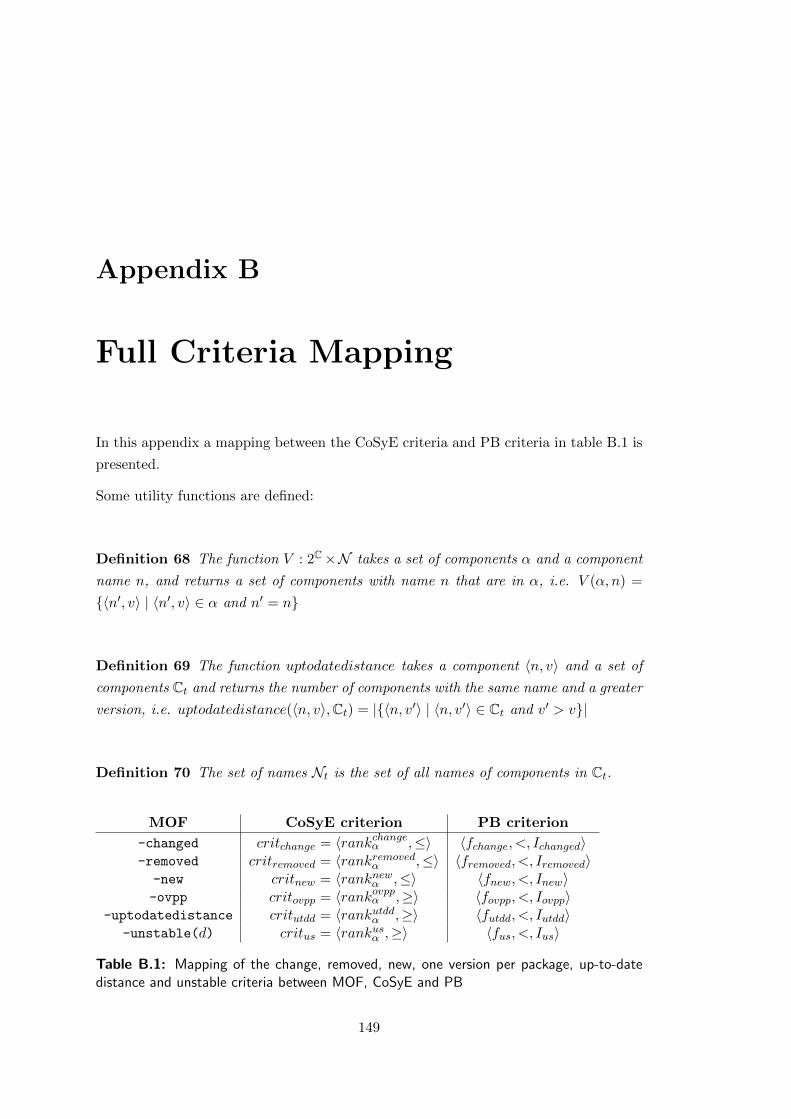
Appendix B
Full Criteria Mapping
In this appendix a mapping between the CoSyE criteria and PB criteria in table B.1 is
presented.
Some utility functions are defined:
Definition 68 The function V : 2C×N takes a set of components α and a component
name n, and returns a set of components with name n that are in α, i.e. V (α, n) =
〈n′, v〉 | 〈n′, v〉 ∈ α and n′ = n
Definition 69 The function uptodatedistance takes a component 〈n, v〉 and a set of
components Ct and returns the number of components with the same name and a greater
version, i.e. uptodatedistance(〈n, v〉,Ct) = |〈n, v′〉 | 〈n, v′〉 ∈ Ct and v′ > v|
Definition 70 The set of names Nt is the set of all names of components in Ct.
MOF CoSyE criterion PB criterion
-changed critchange = 〈rankchangeα ,≤〉 〈fchange, <, Ichanged〉-removed critremoved = 〈rankremovedα ,≤〉 〈fremoved, <, Iremoved〉-new critnew = 〈ranknewα ,≤〉 〈fnew, <, Inew〉-ovpp critovpp = 〈rankovppα ,≥〉 〈fovpp, <, Iovpp〉
-uptodatedistance critutdd = 〈rankutddα ,≥〉 〈futdd, <, Iutdd〉-unstable(d) critus = 〈rankusα ,≥〉 〈fus, <, Ius〉
Table B.1: Mapping of the change, removed, new, one version per package, up-to-datedistance and unstable criteria between MOF, CoSyE and PB
149
APPENDIX B. FULL CRITERIA MAPPING
B.1 -changed
The change criterion is defined:
Definition 71 The change criterion is defined as critchange = 〈rankchangeα ,≤〉, where
rankchangeα (β) = |n | n ∈ N and V (α, n) 6= V (β, n)|.
Definition 72 Given a name n, a component system α, and the set of components
Ct, the auxiliary variable xn is defined with the set of literals l1, . . . , li = V (α, n) ∪¬V (Ct/α, n) such that xn ⇔ l1 ∧ . . .∧ li. This xn can be converted into the set of CNF
clauses Jn = ¬xn, l1, . . . , ¬xn, ln, xn,¬l1, . . . ,¬li.
That is, xn is true only if all components with name n that are installed stay installed
and if not installed stay not installed.
Definition 73 Given a set of names Nt, the PB criterion is defined as 〈fchange, <, Ichanged〉 where fchange is defined with the literals 〈¬xn1 , . . . ,¬xni〉 where 〈n1, . . . , ni〉 =
Nt, and integers 〈11, . . . , 1i〉. The formula Ichanged then equals Jn1 ∪ . . . ∪ Jni.
The PB criterion minimises the sum of names that have changed.
B.2 -removed
The removed criterion is defined:
Definition 74 The removed criterion is defined as critremoved = 〈rankremovedα ,≤〉,where rankremovedα (β) = |n | n ∈ N and V (α, n) 6= ∅ and V (β, n) = ∅|.
Definition 75 Given a name n and the set of components Ct, the auxiliary variable
xn is defined given the set of literals l1, . . . , li = V (Ct, n) such that xn ⇔l1 ∨ . . . ∨ li. This xn can be converted into the set of CNF clauses Jn =
xn,¬l1, . . . , xn,¬ln, ¬xn, l1, . . . , li.
That is, xn is true only if the name n is in the solution.
Definition 76 Given a set of names in the system α is Nα, the PB criterion is defined
as 〈fremoved, <, Iremoved〉 where fremoved is defined with the literals 〈¬xn1 , . . . ,¬xni〉where 〈n1, . . . , ni〉 = Nα, and integers 〈11, . . . , 1i〉. The formula Iremoved then equals
Jn1 ∪ . . . ∪ Jni.
150
APPENDIX B. FULL CRITERIA MAPPING
That is, the PB function sums the total number of names that have been removed from
α.
B.3 -new
The new criterion is defined:
Definition 77 The new criterion is defined as critnew = 〈ranknewα ,≤〉, where
ranknewα (β) = |n | n ∈ N where V (α, n) = ∅ and V (β, n) 6= ∅|.
The new criteria use the same definition of axillary variables from the removed criterion
in definition 75.
Definition 78 Given a set of names that are not in the system α is N6∈α, the PB
criterion is defined as 〈fremoved, <, Iremoved〉 where fnew is defined with the literals
〈xn1 , . . . , xni〉 where 〈n1, . . . , ni〉 = N6∈α, and integers 〈11, . . . , 1i〉. The formula Inew
then equals Jn1 ∪ . . . ∪ Jni.
That is, the PB function sums the total number of names that have been added to α.
B.4 -uptodatedistance
The UTTD criteria is defined:
Definition 79 Given the set of components Ct, the uptodate distance criterion is
defined as critutdd = 〈rankutddα ,≥〉, where rankutddα (β) =∑
c∈β uptodatedistance(c,Ct).
No axillary variables are required for this criteria.
Definition 80 Given the set of components Ct the PB criterion is defined as
〈futdd, <, Iutdd〉 where futdd is defined with the literals l1, . . . , li = Ct, and integers
〈uptodatedistance(l1,Ct), . . . , uptodatedistance(li,Ct)〉. The formula Iutdd then equals
∅.
That is, the sum of the uptodatedistance for each component that is installed in the
system (where the literal is positive) is the returned value of futdd.
151
APPENDIX B. FULL CRITERIA MAPPING
B.5 -ovpp
The one version per package criterion is defined as:
Definition 81 Given the set of components Ct, the One Version per Package
criterion is defined as critovpp = 〈rankovppα ,≥〉, where rankovppα (β) =∑
n∈N |V (β, n)| >1.
This criteria is defined to minimise the number of components with more than one
version installed.
Definition 82 Given a name n and the set of components Ct, the auxiliary variable
xn is defined given the set of literals l1, . . . , li = V (Ct, n) such that xn is true iff two
or more of the literals l1, . . . , li are true. This xn is defined using the PB constraint
where the PB function is defined with literals 〈l1, . . . , li〉 tuple of integers 〈11, . . . , 1i〉,the relationship is > and the integer k = 1.
That is, xn is true only if their are two components, both with name n installed.
Definition 83 Given the set of names Nt, the PB criterion is defined as 〈fovpp, <, Iovpp〉 where fovpp is defined with the literals 〈xn1 , . . . , xni〉 where 〈n1, . . . , ni〉 = Nt,and integers 〈11, . . . , 1i〉. The formula Iovpp then equals Jn1 ∪ . . . ∪ Jni.
B.6 -unstable(d)
The unstable criterion uses the stable function, from definition 39, to minimise the
number of unstable components.
Definition 84 Given a number of days d, a set of components Ct, and the function
stable(c, d, t) is modified to return 1 instead of true and 0 instead of false, the
unstable PB criterion is defined as 〈fus, <, Ius〉 where fus is defined with the literals
l1, . . . , li = Ct, and integers 〈stable(l1, d, t), . . . , stable(li, d, t)〉. The formula Ius
equals ∅.
152
Bibliography
P Abate and R DiCosmo. MPM: a modular package manager. In Proc. CBSE’2011,
2011.
P. Abate, A. Guerreiro, S. Lauriere, R. Treinen, and S. Zacchiroli. Extension of an
existing package manager to produce traces of ugradeability problems in CUDF
format. Technical report, The Mancoosi Project, 2010.
C.E. Alchourron, P. Gardenfors, and D. Makinson. On the logic of theory change:
Partial meet contraction and revision functions. Journal of symbolic logic, 50(2):
510–530, 1985. ISSN 0022-4812.
A. Aleti, L. Grunske, I. Meedeniya, and I. Moser. Let the Ants Deploy Your Software:
an ACO Based Deployment Optimisation Strategy. In Proc. ASE’2009, pages 505–
509. IEEE Press, 2009.
Andreas Barth, Adam Di Carlo, Raphael Hertzog, and Christian Schwarz. Debian
developer’s reference. Technical report, 2005.
K. Bennett. Legacy systems: coping with stress. IEEE Software, 12(1):19–23, 1995.
ISSN 07407459.
Keith H. Bennett and Vaclav T. Rajlich. Software Maintenance and Evolution: a
Roadmap. In ICSE ’2000, pages 73–87, New York, New York, USA, May 2000.
ACM Press. ISBN 1581132530.
J. Bisbal, D. Lawless, and J. Grimson. Legacy information systems: issues and
directions. IEEE Software, 16(5):103–111, 1999. ISSN 07407459.
B. W. Boehm. A spiral model of software development and enhancement. Computer,
21(5):61–72, May 1988. ISSN 00189162.
Frederick P Brooks. The Mythical Man-Month. Addison Wesley, 1975.
Daniel Burrows. Modelling and Resolving Software Dependencies. Technical report,
Debian, June 2005.
153
BIBLIOGRAPHY
R.J. Calistri-Yeh. Iterative strengthening: An algorithm for generating anytime optimal
plans. In Tools with Artificial Intelligence’1994, pages 728–731. IEEE, 1994.
J Chen, H Wang, Y Zhou, and S Bruda. Complexity Metrics for Component-based
Software Systems. Digital Content Technology and its Applications, 5(3), 2011.
SA Cook. The complexity of theorem-proving procedures. In Proc. STOC ’1971, 1971.
Ivica Crnkovic, Severine Sentilles, Vulgarakis Aneta, and Michel R.V. Chaudron. A
Classification Framework for Software Component Models. IEEE Transactions on
Software Engineering, 37(5):593–615, September 2011. ISSN 0098-5589.
M. Davis, G. Logemann, and D. Loveland. A machine program for theorem-proving.
Communications of the ACM, 5(7):394–397, 1962.
Martin Davis and Hilary Putnam. A Computing Procedure for Quantification Theory.
Journal of the ACM, 7(3):201–215, July 1960. ISSN 00045411.
E. S de Almeida, D. Lucredio, and A. F Prado. A survey on software components search
and retrieval. Proc. Euromicro 2004, 0:152–159, September 2004. ISSN 1089-6503.
Greg Dennis, Felix ShengHo, and Chang Daniel Jackson. Modular verification of code
with SAT. In Proc. ISSTA’2006, page 109, New York, New York, USA, July 2006.
ACM Press. ISBN 1595932631.
J. Dietrich, V. Yakovlev, C. McCartin, G. Jenson, and M. Duchrow. Cluster analysis
of Java dependency graphs. In Proceedings of the 4th ACM Symposium on Software
Visualization, pages 91–94. ACM, 2008.
H. Dixon. Automating Pseudo-Boolean Inference Within a DPLL Framework. PhD
thesis, 2004.
M. A. Fortuna, J. A. Bonachela, and S. A. Levin. Evolution of a modular software
network. Proceedings of the National Academy of Sciences, November 2011. ISSN
0027-8424.
M. Fowler and K. Beck. Refactoring: improving the design of existing code. Addison-
Wesley Professional, 1999.
Mike Gancarz. Linux and the Unix philosophy. Digital Press, 2003. ISBN 1555582737.
B Ganter and R Wille. Formal concept analysis. Springer-Verlag, 1999.
John Gary Gaschnig. Performance measurement and analysis of certain search
algorithms. January 1979.
154
BIBLIOGRAPHY
Michael W. Godfrey and Daniel M. German. The past, present, and future of
software evolution. In 2008 Frontiers of Software Maintenance, pages 129–138. IEEE,
September 2008. ISBN 978-1-4244-2654-6.
Charles Gouin-Vallerand and Sylvain Giroux. Managing and Deployment of
Applications with OSGi in the Context of Smart Home. WiMob’2007, pages 70–
70, October 2007.
P Grubb and AA Takang. Software maintenance: concepts and practice. 2003.
Jiang Guo and Luqi. A Survey of Software Reuse Repositories. In Proc. ECBS’2000,
pages 92–100. IEEE Press, 2000. ISBN 0-7695-0604-6.
G.T. Heineman and W.T. Councill. Component-based software engineering: putting the
pieces together, volume 17. Addison-Wesley USA, 2001.
Petr Hnetynka and F Plasil. Dynamic reconfiguration and access to services in
hierarchical component models. Component-Based Software Engineering, 2006.
IEEE. IEEE standard glossary of software engineering terminology. 1990.
ISO/IEC. ISO/IEC 14764 IEEE Std, Software Engineering-Software Life Cycle
Processes-Maintenance. 2006.
Graham Jenson, Jens Dietrich, and Hans W. Guesgen. An Empirical Study of the
Component Dependency Resolution Search Space. In Proc. CBSE’2010, pages 182–
199. Springer, 2010a.
Graham Jenson, Jens Dietrich, and Hans W. Guesgen. A Formal Framework to
Optimise Component Dependency Resolution. In Proc. APSEC’2010. IEEE, 2010b.
Graham Jenson, Jens Dietrich, Hans W. Guesgen, and Stephen Marsland. An empirical
study into component system evolution. In Proc. CBSE’2011, Boulder, CO, 2011.
ACM.
Marques-Silva Joao, Josep Argelich, Ana Graca, and Ines Lynce. Boolean lexicographic
optimization: algorithms & applications. Annals of Mathematics and Artificial
Intelligence, 62(3):317–343, 2011.
Changwoo Jung. Short Talk Integrating OSGi Bundle Repository ( OBR ) inside Eclipse
for Bundle Deployment. Computing, pages 1–11, 2007.
ChangWoo Jung and Han Chen. Embedded device solution life cycle support with
Eclipse. OOPSLA’2006 Workshop on eclipse, pages 1–5, 2006.
155
BIBLIOGRAPHY
Peter Kriens. How OSGi Changed My Life. Queue, 6(1):44–51, 2008. ISSN 1542-7730.
C.K. Kwong, L.F. Mu, J.F. Tang, and X.G. Luo. Optimization of software components
selection for component-based software system development. Computers & Industrial
Engineering, 58(4):618–624, May 2010. ISSN 03608352.
Averill M. Law. How to build valid and credible simulation models. In Proc. WSC ’05,
pages 24–32, December 2005. ISBN 0-7803-9519-0.
D. Le Berre and A. Parrain. The Sat4j library, release 2.2 system description. Journal
on Satisfiability, Boolean Modeling and Computation, 7:59–64, 2010.
Daniel Le Berre and Anne Parrain. On SAT Technologies for Dependency Management
and Beyond. In Proc. SPLC’2008, pages 197–200. Lero Int. Science Centre, 2008.
Meir M. Lehman and Juan F. Ramil. Software evolution - Background, theory, practice.
Information Processing Letters, 88(1-2):33–44, October 2003. ISSN 00200190.
MM Lehman. The programming process. Technical report, 1969.
M.M. Lehman. Programs, life cycles, and laws of software evolution. Proc. IEEE, 68
(9):1060–1076, 1980. ISSN 0018-9219.
Liangming Li, Zhijian Wang, and Xuejie Zhang. An Approach to Testing Based
Component Composition. ISECS’2008, pages 735–739, August 2008.
BP Lientz and EB Swanson. Software Maintenance Management: A Study
of the Maintenance of Computer Application Software in 487 Data Processing
Organizations. 1980.
Shengyuan Luo, Jin Zhu, and Ping Jiang. Software Evolution of Robot Control Based
on OSGi. ROBIO’2004, 0:221–226, August 2004.
C.F. Madigan, M.H. Moskewicz, and S. Malik. Efficient conflict driven learning in a
Boolean satisfiability solver. In ICCAD’2001, pages 279–285. IEEE, 2001. ISBN
0-7803-7247-6.
Fabio Mancinelli, Jaap Boender, Roberto Cosmo, Jerome Vouillon, Berke Durak, Xavier
Leroy, and Ralf Treinen. Managing the Complexity of Large Free and Open Source
Package-Based Software Distributions. In ASE’2006, pages 199–208. IEEE, 2006.
ISBN 0-7695-2579-2.
Joao P. Marques-Silva and Karem A. Sakallah. Boolean satisfiability in electronic design
automation. In Proc. DAC ’00, pages 675–680, New York, New York, USA, June
2000. ACM Press. ISBN 1581131879.
156
BIBLIOGRAPHY
J. McAffer, P. VanderLei, and S. Archer. OSGI and Equinox: Creating highly modular
Java systems. Addison-Wesley Professional, 2010.
M. D McIlroy. Mass produced software components. Software Engineering: Report of
a conference sponsored by the NATO Science Committee, 1969.
M.D. McIlroy. Pipes and filters. Internal Bell Labs memo, original title lost, 11, 1964.
Bertrand Meyer. The Significance of Components. Dr. Dobb’s, November 1999.
Bertrand Meyer. What to Compose. Dr. Dobb’s, March 2000.
Anders Mørch. Three levels of end-user tailoring: customization, integration, and
extension. Computers and design in context, 1997.
Matthew W. Moskewicz, Conor F. Madigan, Ying Zhao, Lintao Zhang, and Sharad
Malik. Chaff: engineering an efficient SAT solver. In Proc. DAC ’01, pages 530–535,
New York, New York, USA, June 2001. ACM Press. ISBN 1581132972.
I. Murdock. A brief history of Debian. Appendix A, The Debian Manifesto, Revised
January, 6, 1994.
Ian Murdock. How package management changed everything, 2007. URL http:
//ianmurdock.com/solaris/how-package-management-changed-everything/.
E Murphy-Hill and AP Black. Refactoring tools: Fitness for purpose. Software, IEEE,
2008.
Niklas Sorensson Niklas Een. An Extensible SAT-solver [ver 1.2]. Theory and
Applications of Satisfiability Testing, 2004.
Online Oxford English Dictionary. Oxford English Dictionary Online. Technical Report
07/07, 2010. URL http://dictionary.oed.com.
Michael P. Papazoglou, Vasilios Andrikopoulos, and Salima Benbernou. Managing
Evolving Services. IEEE Software, 28(3):49–55, May 2011. ISSN 0740-7459. doi:
10.1109/MS.2011.26.
D. L. Parnas. On the criteria to be used in decomposing systems into modules.
Communications of the ACM, 15(12):1053–1058, December 1972. ISSN 00010782.
B. Porter, C. Sanchez, J. Casey, and V. Massol. Better Builds with Maven. MaestroDev,
2008.
R. Prieto-Diaz and P. Freeman. Classifying Software for Reusability. IEEE Software,
4(1):6–16, January 1987. ISSN 0740-7459.
157

BIBLIOGRAPHY
Vivien Quema, Thierry Coupaye, Jean-Bernard Stefani, Eric Bruneton, and Matthieu
Leclercq. The FRACTAL component model and its support in Java. Software:
Practice and Experience, 36:1257–1284, 2006.
Pascal Rapicault and Daniel Le Berre. Dependency Management for the Eclipse
Ecosystem. In Proc. IWOCE’2009. ACM, August 2009.
Pascal Rapicault and Daniel Le Berre. Dependency Management for the Eclipse
Ecosystem: An Update. In Proc. LaSh’2010, 2010.
E.S. Raymond. The Art of Unix Programming. Pearson Education, 2003.
A. Ryan and J. Newmarch. An architecture for component evolution. CCNC’2005, 0:
498–503, January 2005.
PH Salus. A Quarter century of UNIX. 1994. URL http://www.slac.stanford.edu/
spires/find/books?irn=271780.
Juha Savolainen, Ian Oliver, Varvana Myllarniemi, and Tomi Mannisto. Analyzing and
Re-structuring Product Line Dependencies. In Proc. COMPSAC’2007, volume 1,
pages 569–574. IEEE Press, 2007.
Thomas J. Schaefer. The complexity of satisfiability problems. In Proc. STOC ’78,
pages 216–226, New York, New York, USA, May 1978. ACM Press.
B Selic. The pragmatics of model-driven development. Software, IEEE, 2003.
Hossein M. Sheini and Karem A. Sakallah. Pueblo: A hybrid pseudo-boolean SAT
solver. August 2006.
Niklas Sorensson, Armin Biere, and Oliver Kullmann. Theory and Applications of
Satisfiability Testing - SAT 2009, volume 5584 of Lecture Notes in Computer Science.
Springer Berlin Heidelberg, Berlin, Heidelberg, 2009. ISBN 978-3-642-02776-5.
R. Stallman and Others. The GNU manifesto. Dr. Dobb’s, 10(3):30–35, 1985. URL
http://www.gnu.org/gnu/manifesto.html.
Richard M. Stallman and Gerald Jay Sussman. Forward Reasoning and Dependency-
Directed Backtracking in a System for Computer-Aided Circuit Analysis. September
1976.
Alexander Stuckenholz. Component Updates as a Boolean Optimization Problem. In
Electronic Notes in Theoretical Computer Science, volume 182, pages 187–200, June
2007.
158
BIBLIOGRAPHY
Clemens Szyperski. Point, Counterpoint. Dr. Dobb’s, February 2000a.
Clemens Szyperski. Components and Contracts. Dr. Dobb’s, May 2000b.
Clemens Szyperski. Component Software: Beyond Object-Oriented Programming. The
Component Software Series. Addison-Wesley Longman Publishing Co., Boston, MA,
USA, 2nd edition, 2002. ISBN 0201745720.
A.S. Tanenbaum. MINIX Operating System. Japan, Apr, 21:328, 1989.
The Agile Alliance. Manifesto for Agile Software Development, 2001. URL http:
//agilemanifesto.org/.
The OSGi Alliance. RFC-0112 Bundle Repository. 2006.
The OSGi Alliance. OSGi Service Platform Service Compendium. April 2007a. URL
http://www.osgi.org/Specifications/.
The OSGi Alliance. OSGi Service Platform Core Specification. April 2007b. URL
http://www.osgi.org/Specifications/.
L. Torvalds and D. Diamond. Just for fun: The story of an accidental revolutionary.
Harper Paperbacks, 2002.
R. Treinen and S. Zacchiroli. Common upgradeability description format (CUDF) 2.0.
Technical report, 2009a. URL http://www.mancoosi.com/reports/tr3.pdf.
Ralf Treinen and Stefano Zacchiroli. Expressing advanced user preferences in
component installation. In IWOCE ’09, Amsterdam, 2009b.
R. Vasa, M. Lumpe, and J.G. Schneider. Patterns of component evolution. In SC’2012,
pages 235–251. Springer-Verlag, 2007.
Damien Watkins, Jean-Marc Jezequel, Noel Plouzeau, and Antoine Beugnard. Making
Components Contract Aware. Computer, 32(7):38–45, 1999. ISSN 0018-9162.
Jin Xinjuan, Long Yihong, and Liu Quan. Research on Ontology-based Representation
and Retrieval of Components. SNPD’2007, 1:494–499, August 2007.
E. Yourdon and L. L. Constantine. Structured design. Yourdon, 1976.
159