Embed Size (px)
Citation preview

June 2010Nils A. Baas, MATH
Master of Science in MathematicsSubmission date:Supervisor:
Norwegian University of Science and TechnologyDepartment of Mathematical Sciences
A Study and Comparison of First andSecond Order Cellular Automata withExamples
Lauritz Vesteraas Thaulow


Problem Description
First give a general introduction to cellular automata, then implement and discuss someexamples. Introduce higher order cellular automata, examine whether and how the ex-amples can be extended by applying 2-dynamics and/or 2-morphology, and study theeects.


Preface
This diploma thesis is the conclusion of my masters degree at the Norwegian Universityof Science and Technology.
I would like to thank my supervisor, Professor Nils A. Baas for his help and input,and my fellow master student Pål Davik, who has been writing a diploma on the samesubject this year, for inspiration and support.
Trondheim, June 2010Lauritz Vesteraas Thaulow


Abstract
This thesis will give an introduction to the concepts of cellular automata and higherorder cellular automata, and go through several examples of both. Cellular automataare discrete systems of cells in an n-dimensional grid. The cells interact with each otherthrough the use of a rule depending only on local characteristics, which lead to someglobal behaviour. Higher order cellular automata are hierarchical structures of cellularautomata with added possibilities for dynamic local interaction.
We rst give an introduction for non-mathematicians. A mathematical denition ofcellular automata follows, and we illustrate the many possibilities with a few examples.
Higher order cellular automata are introduced and dened, and we look at the conse-quences higher order cellular automata has on optimization of computer implementations.Finally we apply higher order structures to some of the examples, and study the eects.

vi

Contents
Notation and Abbreviations . . . . . . . . . . . . . . . . . . . . . . . . . . . . . 1
Introduction . . . . . . . . . . . . . . . . . . . . . . . . . . . . . . . . . . . . . . 3
1 Cellular Automata 5
1.1 Introduction . . . . . . . . . . . . . . . . . . . . . . . . . . . . . . . . . . . 5
1.1.1 A kind of machine . . . . . . . . . . . . . . . . . . . . . . . . . . . 5
1.1.2 Rule 30 from the inside . . . . . . . . . . . . . . . . . . . . . . . . 6
1.1.3 Giving names to the concepts . . . . . . . . . . . . . . . . . . . . . 7
1.2 History . . . . . . . . . . . . . . . . . . . . . . . . . . . . . . . . . . . . . 10
1.2.1 A self-reproducing automaton . . . . . . . . . . . . . . . . . . . . . 10
1.2.2 The Game of Life . . . . . . . . . . . . . . . . . . . . . . . . . . . . 10
1.2.3 Stephen Wolfram . . . . . . . . . . . . . . . . . . . . . . . . . . . . 11
1.3 Formal denition . . . . . . . . . . . . . . . . . . . . . . . . . . . . . . . . 12
1.3.1 Cellular automata . . . . . . . . . . . . . . . . . . . . . . . . . . . 12
1.3.2 The local transition function . . . . . . . . . . . . . . . . . . . . . 12
1.3.3 The global function . . . . . . . . . . . . . . . . . . . . . . . . . . . 12
1.3.4 Reversibility, support and the Garden of Eden . . . . . . . . . . . . 13
1.3.5 Neighbourhoods . . . . . . . . . . . . . . . . . . . . . . . . . . . . 14
1.3.6 Wolfram numbering . . . . . . . . . . . . . . . . . . . . . . . . . . 14
1.4 Examples . . . . . . . . . . . . . . . . . . . . . . . . . . . . . . . . . . . . 18
1.4.1 1-dimensional binary cellular automata . . . . . . . . . . . . . . . . 18
1.4.2 Other 1-dimensional cellular automata . . . . . . . . . . . . . . . . 23
1.4.3 Activation-inibition model . . . . . . . . . . . . . . . . . . . . . . . 27
1.4.4 The Game of Life . . . . . . . . . . . . . . . . . . . . . . . . . . . . 30
1.4.5 The hodgepodge machine . . . . . . . . . . . . . . . . . . . . . . . 33
1.4.6 WATOR-World . . . . . . . . . . . . . . . . . . . . . . . . . . . . . 37
2 Higher Order Cellular Automata 43
2.1 Introduction . . . . . . . . . . . . . . . . . . . . . . . . . . . . . . . . . . . 43
2.2 Denition . . . . . . . . . . . . . . . . . . . . . . . . . . . . . . . . . . . . 44
2.2.1 2-dynamics . . . . . . . . . . . . . . . . . . . . . . . . . . . . . . . 44
2.2.2 2-morphology . . . . . . . . . . . . . . . . . . . . . . . . . . . . . . 45
2.3 Problems of optimization . . . . . . . . . . . . . . . . . . . . . . . . . . . 47
2.4 Examples . . . . . . . . . . . . . . . . . . . . . . . . . . . . . . . . . . . . 49
vii
viii CONTENTS
2.4.1 1-dimensional cellular automata . . . . . . . . . . . . . . . . . . . . 492.4.2 The Game of Life . . . . . . . . . . . . . . . . . . . . . . . . . . . . 542.4.3 Hodgepodge and activition-inhibition . . . . . . . . . . . . . . . . . 572.4.4 WATOR-World . . . . . . . . . . . . . . . . . . . . . . . . . . . . . 58
3 Conclusions 63
References 66
A Application documentation 67
A.1 General documentation . . . . . . . . . . . . . . . . . . . . . . . . . . . . . 67A.2 Prerequisites . . . . . . . . . . . . . . . . . . . . . . . . . . . . . . . . . . 67A.3 Vector graphics cellular automata . . . . . . . . . . . . . . . . . . . . . . . 68A.4 CA Explorer . . . . . . . . . . . . . . . . . . . . . . . . . . . . . . . . . . . 68A.5 Game of Life . . . . . . . . . . . . . . . . . . . . . . . . . . . . . . . . . . 69A.6 Hodgepodge . . . . . . . . . . . . . . . . . . . . . . . . . . . . . . . . . . . 69A.7 WATOR-World . . . . . . . . . . . . . . . . . . . . . . . . . . . . . . . . . 70A.8 HOCA . . . . . . . . . . . . . . . . . . . . . . . . . . . . . . . . . . . . . . 70
B Radius 1 binary 1-CA 71
Index 75

CONTENTS 1
Notation and Abbreviations
Throughout this paper, the notation listed below will be used.
S, N Upper-case letters denote setsN , R Script upper-case letters are mostly used to denote sets of setsa, n Bolded letters are mapsc, s Lower-case letters are single values or functions~z ~z is a vector and zi is its ith axial component
(a, b) (a, b) is a vector or tuple with each axial component explicitlyspecied, and is equal to
[ab
]a, b, c a, b, c is a set with the elements a, b and c
Z The set of all integersZ+ The set of non-negative integers 0, 1, 2, . . . Zn The set 0, 1, 2, . . . , n− 1Sn The set S × S × . . .× S︸ ︷︷ ︸
n times
P(S) The set of all nite subsets of S.|S| The cardinality of the set S, Card(S)bxe The nearest integer of xbxc The integer part of x
~a+~b Vector addition, equals (a0 + b0, a1 + b, . . . , ad−1 + bd−1)for d-dimensional vectors ~a and ~b.
‖~z‖1 The manhattan norm, ‖~z‖1 =∑m
i=1 |zi|for an m-dimensional vector ~z.
‖~z‖∞ The maximum norm, ‖~z‖∞ = max|zi| | i ∈ 1, . . . ,mfor an m-dimensional vector ~z.
g h The function g composed with the function h, so that (g h)(x) = g(h(x)).
And these are the most commonly used abbreviations:
CA cellular automatonHOCA higher order cellular automatonLTF local transition functiond-CA d-dimensional cellular automatonIBM individual-based modelCPU central processing unitRAM random access memory

2 CONTENTS

CONTENTS 3
Introduction
How does complexity arise from simple beginnings? The universe was born, accordingto astrophysicists, from extremely uniform and well-ordered beginnings, yet the result isstaggeringly complex. Smoke rising from a blown out candle is orderly and simple, untilit suddenly becomes chaotic and unpredictable.
New Scientist wrote in its article Seven questions that keep physicists up at night [17]:
From the unpredictable behaviour of nancial markets to the rise of lifefrom inert matter, Leo Kadanano, physicist and applied mathematician atthe University of Chicago, nds the most engaging questions deal with therise of complex systems. Kadano worries that particle physicists and cos-mologists are missing an important trick if they only focus on the very smalland the very large. "We still don't know how ordinary window glass worksand keeps it shape," says Kadano. "The investigation of familiar things isjust as important in the search for understanding." Life itself, he says, willonly be truly understood by decoding how simple constituents with simpleinteractions can lead to complex phenomena.
Cellular automata are prime examples of systems with simple constituents and simpleinteractions which lead to complex phenomena, and they are exellently suited for detailedstudy and analysis on exactly how it happens, because they can be simulated easily in acomputer.
In this thesis we will use the rst chapter to introduce, dene and give examplesof cellular automata, and show how the very simple can quickly become very complex,even though every step on the way is obvious and simple. We will also give examples ofcellular automata that simulate processes from real life, some with very accurate results.
In chapter 2 we will introduce the concept of higher order cellular automata. We willconsider what consequences adding higher order structures and 2-dynamics have on ourability to optimize computer implementations of such cellular automata. Finally, we willapply higher order structures or 2-dynamics to some of the examples from chapter 1, andconsider the eects.

4 CONTENTS

Chapter 1
Cellular Automata
1.1 Introduction
The concept of a cellular automaton is rather simple. However, the use of mathemat-ical notation and lingo in this and other papers, makes it unnecessarily hard for non-mathematicians to grasp. This section is therefore written in a more informal language, asa gentle introduction on the subject, for those who have little or no higher mathematicaleducation.
1.1.1 A kind of machine
A cellular automaton is like a machine you can put something into it, and it will usethat input to produce some output. In our case, this machine is going to take rows ofblack and white squares as input, and produce an equally long row of black and whitesquares as output.
Figure 1.1: A cellular automaton
5

6 CHAPTER 1. CELLULAR AUTOMATA
Figure 1.1 is an image produced by a cellular automaton called rule 30 . The topmostrow, with a single black square, is used as the input to rule 30, and it produces the secondrow as output. We then use that row as a new input to the same rule, and get the thirdrow as output, and so on.
Rule 30 is just one example of a cellular automaton. They come in a huge variety ofshapes and sizes. This text will rst tell you how to make such patterns of your own,using only pen and paper. Then, for those who wish to read more on the subject, anintroduction to the lingo of cellular automata will be given, based on the concepts we'veused.
1.1.2 Rule 30 from the inside
Figure 1.2: The instructions
Imagine you were given a sheet of graph paper as in 1.2. The paper contains a row of7 instructions, which we will use to create the same pattern as in gure 1.1. This means,of course, that the 7 instructions correspond to rule 30, but we need to understand howto use them.
To that end, you've been given a loose piece of transparency (also shown in gure1.2), on which a gure has been drawn in black ink. Inside the smallest box a hole hasbeen cut through the plastic. The piece of transparency can be moved around, so imaginethat you place it as in the left image of gure 1.3. Now notice that the pattern in thethree squares outlined in black matches those in the instruction numbered 7 in gure 1.2.However, that drawing also has a cross in the square hanging underneath, so they donot match completely... yet. The transparency has a convenient hole where the missingcross should be, so we draw an there to make them equal.
Continuing, we move the transparency one square to the right, as shown to the right ofgure 1.3, and observe that the upper three squares now has content matching instruction6. This also has an in the square underneath, so we draw an where the hole is, tomake them similar. Finally we move the transparency to the right once more and useinstruction number 4 to place another on the graph paper, which is now looking likein gure 1.4 to the left.
For the next row, we'll need to use instructions 7, 5, 1, 2 and 4, and this will produce

1.1. INTRODUCTION 7
Figure 1.3: Using the piece of transparency.
Figure 1.4: The second and third row.
a drawing like the one to the right in gure 1.4. Continuing like this for a while we'll geta drawing like the one in gure 1.5. Notice that the order in which we calculated therows of squares did not matter, we could have done them right-to-left, or in an arbitraryorder, instead of left-to-right.
Figure 1.5: After 18 rows.
We can now easily see the similartiy between our drawing and gure 1.1. As indicatedby the number 30 in rule 30, it is but one of many such rules1.
1.1.3 Giving names to the concepts
We've now presented the basic parts of a cellular automaton, but we still have notwritten down exactly what it is. A cellular automaton is made up of exactly four piecesof information:
• An alphabet : the dierent symbols we can use; for us it was only two, and .
• A lattice: the rows of squares that we draw on.
1The logic behind the numbering is explained in section 1.3.6

8 CHAPTER 1. CELLULAR AUTOMATA
• A neighbourhood : the three squares that were outlined by our transparency, andhow they're positioned relative to the hole we may draw an in.
• A function or rule: tells us what symbol to draw in every case, like our 7 instruc-tions.
Each square is called a cell, and each symbol, like and , is called a state. We saythat the cell has a state. The cellular automaton we've drawn is called a 1-dimensionalcellular automaton, even though the drawing we've made lls a two-dimensional grid.This is because we regard the vertical axis as time, with time increasing downwards. Sojust like we live in a three-dimensional world with time, this cellular automaton livesin a 1-dimensional world with time. Each row is then the whole world at one particulartime, this world is what we call the lattice. At each time step, the lattice has a particularpattern of states, and each such pattern is called a global state or conguration.
The three cells in a row that was our neighbourhood can contain eight dierentpatterns2 of 's and 's, and each of these patterns we will call a neighbourhood state.It might be tempting to call it a neighbourhood conguration instead, but this term willbe needed for something else later.
The neighbourhood concept is perhaps a little dicult to grasp, since it may seem tobe just a part of what makes up a rule. It really isn't, though the two concepts dependon each other to some degree. In our example, the neighbourhood was the three cells ina row, centered on the one we were to nd the new state of. However, we could havechanged the neighbourhood while keeping the rule by for example shifting the three cellsto the right or left, or even by spreading them out so that they are neither adjacent norsymmetric3. The rule needs to be compatible with the neighbourhood though; using ourseven instructions with a neighbourhood consisting of ve cells would make no sense,since there'd be no matching instructions for the neighbourhood states we'd encounter.
Neighbourhoods come in many dierent shapes and sizes, although some are morecommonly used than others. We say that ours had a radius of 1, since it included 1 cellon each side of the cell we were nding the next state for.
We have not talked about what happens when the pattern reaches the edges of thepaper, or lattice. Throughout this thesis we will mostly use lattices that wrap. Thismeans that what goes out on one side, comes in on the other. A way of visualizing thisis of taping the left and right edge of the grid paper together to form a cylinder. Thenthere'd no longer be any edge, and the transparency would be usable all the way around,as illustrated in gure 1.6.
We've now covered the basic concepts that make up a cellular automaton. Thesecan be built upon and extended to make things more interesting. We may add anotherdimension, for example, and get a 2-dimensional cellular automaton. To draw such athing with pen and paper, you would need a book of graph paper, one page for each time
2I purposefully left out one instruction from those in the beginning of this section, which is the
instruction for when there is no 's in any of the cells. This did not matter for that rule, since itimplicitly said to leave such cells alone.
3We'd need to imagine them as being adjacent to match them up with the instructions.

1.1. INTRODUCTION 9
Figure 1.6: What happens on the edges.
step. You would also need a set of instructions for a 2-dimensional cellular automaton,and an initial pattern on the rst page. After drawing some pages, you could look atyour animation by ipping through the pages.
Animations and java applets depicting various cellular automata can be found on theinternet, and they are often fascinating to watch. As a starting point, here are somegoogle searches that gives nice results: Game of Life, forest re cellular automaton,hodgepodge machine, cyclic space and trac cellular automaton.

10 CHAPTER 1. CELLULAR AUTOMATA
1.2 History
1.2.1 A self-reproducing automaton
(a) John von Neumann (b) Stanisªaw Ulam (c) Arthur Walter Burks
Figure 1.7: Important gures from the history of cellular automata. These pictures are in the
public domain.
One of the (many) interests of the Hungarian-born mathematician John von Neumannwas how to create self-replicating automatic factories. At rst he considered how tomake such a thing in practice, using robotics or toy mechanic sets, but he soon found theproblem too complex. After conferring with Stanisªaw Ulam on the matter, he decided tofollow his friends advice and instead consider a simple abstract mathematical model [19,p. 876]. He then devised what is now known as cellular automata (CA), and outlineda particular kind of 2-dimensional CA that would be capable of self replication if setup in a certain way. It was a rather complicated one; each cell could be in one of 29dierent states, with each state having a certain meaning. He went on to outline aninitial conguration consisting of 200 000 cells that he claimed would be able to makecopies of itself.
His work remained unpublished until his death in 1957, but it was edited and pub-lished in 1966 by Arthur Walter Burks [18]. The subject of self-reproducing congurationsof cellular automata caught the interest of others, and simpler examples were soon found;Edgar Frank Codd worked out a variant of von Neumann's original example that neededonly eight states [11, p. 1]. Also, during the 1960s various theorems related to the formalcomputational capabilities of cellular automata were proved.
1.2.2 The Game of Life
The eld of Cellular Automata was given its poster child in 1970, when Martin Gardner4
presented some results of John Conway in his column Mathematical Games in ScienticAmerican. Gardner called the game Life , and it was therefore subsequently knownas Conway's Game of Life. Many readers of the column were inspired to do more or
4Martin Gardner died just 10 days prior to the deadline for this thesis, on May 22, 2010.

1.2. HISTORY 11
(a) Martin Gardner (b) John Conway (c) Stephen Wolfram
Figure 1.8: More important gures from the history of cellular automata. (a) Photograph
by Konrad Jacobs, (b) photograph by Thane Plambeck, (c) photograph by Stephen Faust.
less serious research on the Game of Life, and for three years there was even a quar-terly newsletter dedicated to discoveries about the behaviour of this particular cellularautomaton.
Around the same time, microcomputers became available and aordable, and formany aspiring programmers, the Game of Life was the inspiration for the rst applicationsthey made. However, according to Stephen Wolfram, little of direct scientic value cameof the whole thing:
An immense amount of eort was spent nding special initial conditionsthat give particular forms of repetitive or other behaviour, but virtually nosystematic scientic work was done (perhaps in part because even Conwaytreated the system largely as recreation), and almost without exception onlythe very specic rules of Life were ever investigated. [19, p. 877]
1.2.3 Stephen Wolfram
Apart from his contributions to the eld of cellular automata, Stephen Wolfram is to-day best known as the father of the Mathematica computer algebra system and theWolfram|Alpha5 computational knowledge engine. Back in 1981 he started studying cel-lular automata, and instead of concentrating on one particular cellular automaton, as vonNeumann and the Game of Life enthusiasts had done, he undertook a sweeping survey ofmany kinds of cellular automata, and devised a way to classify any cellular automatoninto one of four classes.
Stephen Wolfram went on to write the controversial [15] 1200 pages long A NewKind of Science [19] in 2002. There he claims that what he calls simple programs, ofwhich cellular automata is one example, will be the basis for a whole new approach andmethodology of science within a number of dierent scientic elds.
5http://www.wolframalpha.com/

12 CHAPTER 1. CELLULAR AUTOMATA
1.3 Formal denition
There is no agreed-upon standard formalisation or notation for cellular automata. Thenotation used in this thesis is based on the formalisations of Delorme and Mazoyer [5],but with modications to allow for later adaption to higher order cellular automata, andsome other small changes that was deemed appropriate.
1.3.1 Cellular automata
We need to dene a few concepts to start with. A lattice is an ordered grid, typically Zd,and we denote it L. A neighbourhood is a nite ordered subset of L, and we denote it byN . A cell is an object which has one state at a time. The set of all allowable states is anite set called the alphabet, denoted by S. There's one cell at each node of the lattice.
Denition. A d-dimensional cellular automaton A (a d-CA) is a 4-tuple (L, S,N, f),where L is a lattice, S is an alphabet, N is a neighbourhood, and f is any functionf : S|N | −→ S.
The alphabet S is very often the set 0, 1, . . . , n−1 or some variation thereof, thoughthis is by no means mandatory. Among the states are, sometimes, distinguished statess, called quiescent states, such that f(s, . . . , s) = s.
For the rest of section 1.3, we'll let (L, S,N, f) be a general d-CA unless otherwisespecied.
1.3.2 The local transition function
The function f : S|N | 7→ S is called a local transition function, abbreviated LTF. The setS|N | is the set of all possible neighbourhood states. Each element of S|N | is an orderedset of states s0, s1, . . . , s|N |−1. For some cellular automata, the LTF can be denedwith a formula, for example f(s0, s1, s2) = s0 + s1 + s2 (mod 2). In this case, S is mostoften a subset of the integers (though it can be any nite set on which the necessarymathematical operations are dened).
In other cellular automata, the LTF is so unwieldy that there is no practical wayto express it as a formula, and it may then be necessary to fall back to dening it byexplicitly tabulating all the values in the domain and their associated value in the range.This is not always practicly possible, however. Even though the domain has to be nite,it can be so large that no computer currently in existence could store a function on itin tabular form. Some of these types of cellular automata can fortunately be studied inspite of this, namely those whose LTF can be dened as a computer algorithm. Such analogrithm can be almost arbitrarily complex, and have a large number of parameters.
1.3.3 The global function
A cellular automaton evolves with time. The states of all the cells in the lattice areupdated simultaneously, so that time is discrete. We dene a function at : L −→ S

1.3. FORMAL DEFINITION 13
that gives the state of each cell of the lattice at time t. We call at the global state orconguration at time t, and denote the state of the cell at ~z by at(~z). The sequence(a0,a1,a2, . . . ) is called the behaviour, action or evolution of the cellular automaton.
For a cellular automaton A = (L, S,N, f) with neighbourhood N = ~n0, . . . , ~nn−1,we dene at+1 as the global state such that the following statement is true:
at+1(~z) = f(at(~z + ~n0),at(~z + ~n1), . . . ,at(~z + ~nn−1)) for all ~z ∈ L.
We say that at+1 follows at. We can construct a function G such that G(at) = at+1.We call G the global function of A, as it maps each global state to the global state thatfollows it. Each cellular automaton has its own associated global function.
The domain of G is the set of all possible global states that the cellular automatonmight have, which is equal to S|L|. We denote this set by C. The function G is obviouslyan endofunction of C, that is, G : C −→ C.
In this thesis we'll adopt this convention: if we need to refer to multiple unrelatedelements of the set C, we will use subscripted numbers instead of superscripted numbers.This is to distinguish global states that are part of the evolution of a cellular automatonfrom global states that are unrelated, or might be. For example, a0,a1 ∈ C implies thatG(a0) = a1, while a0,a1 ∈ C does not put any restriction on the relationship betweena0 and a1.
1.3.4 Reversibility, support and the Garden of Eden
It is now natural to consider the properties of the global function. The congurations thatare not in the codomain of G are called the Garden-of-Eden congurations, because theycan only appear as initial conditions, and will never appear during the evolution of thecellular automaton. If a global function G is bijective, and if G−1 is the global function ofsome cellular automaton, we say that both are the global function of a reversible cellularautomaton. It is easy to show that a reversible cellular automaton has no Garden-of-Edencongurations.
For a cellular automaton with a quiescent state s, we dene the support of a cong-uration a as follows:
supp(a) = ~z | a(~z) 6= s
In words, the support of a is the subset of L that has cells with non-quiescent states. Wenow dene a nite conguration as a conguration with nite support. This denitionis used in the following theorem, due to Edward F. Moore and John Myhill:
Theorem 1.3.1 (Garden-of-Eden Theorem). A cellular automaton with a quiescentstate is surjective if and only if it is injective when restricted to nite congurations.
For nite congurations, an injective global function is necesseraly also surjective,because the global function must be dened for every element in the domain, and thedomain and the codomain is the same size, since the global function is an endofunction.

14 CHAPTER 1. CELLULAR AUTOMATA
Conversely, a surjective global function must be injective because the domain equals thecodomain.
Another way of stating this theorem is that a nite cellular automaton with a quies-cent state has a Garden-of-Eden conguration if and only if there exists two congurationsaa and ab ∈ C such that G(aa) = G(ab).
1.3.5 Neighbourhoods
First we will address the question on whether the neighbourhood includes the cell whoseneighbourhood it is (~0) or not. Dierent conventions exists [5, p. 7], but we choose inthis thesis to use neighbourhoods that explicitly includes the cell itself.
The most frequently used neighbourhood for one-dimensional cellular automata isreferred to as the rst neighbours neighbourhood . It consists simply of the central cell ofthe neighbourhood, plus its right and left neighbours: −1, 0, 1. Extending this concept,we get the radius neighbourhood , which we will denote Nr:
−r,−r + 1, . . . ,−1, 0, 1, . . . , r − 1, r
For anm-dimensional cellular automaton wherem > 1, there are two neighbourhoodsthat needs to be mentioned. Recall6 that for a vector ~z, we have the manhattan norm‖~z‖1 and the maximum norm ‖~z‖∞. From these two we get the associated metrics d1
and d∞, which we can use to dene the von Neumann neighbourhood NvN and the Mooreneighbourhood NM , respectively:
NvN (~z) = ~x | ~x ∈ Zd, d1(~z, ~x) ≤ 1 with a given order
NM (~z) = ~x | ~x ∈ Zd, d∞(~z, ~x) ≤ 1 with a given order
In 1 dimension, the von Neumann and Moore neighbourhoods are identical to theradius 1 neighbourhood. The 2-dimensional variants are depicted in gure 1.9. We needto give the elements of the neighbourhoods an order, as we've done for the rst neighboursand radius neighbourhoods. Since we will only use the 2-dimensional variants, we willonly specify the order for those. We'll let the rst element be the origin (0, 0), and thenlet the rest of the elements follow, starting with (1, 0) and going in a counterclockwisedirection.
1.3.6 Wolfram numbering
As mentioned in section 1.3.2, the domain of the local transition function S|N | is a setof ordered sets of the form s0, s1, . . . , s|N |−1, where si ∈ S. If we give S a total order
relation, we may order the set S|N | lexicographically in descending order, making it an
6See page 1.

1.3. FORMAL DEFINITION 15
Figure 1.9: The 2-dimensional von Neumann (left) and Moore (right) neighbourhoods.The black cell is the central cell the cell whose neighbourhood is depicted and it isalso part of the neighbourhood.
ordered set of ordered sets. For example, if S = Z2 and |N | = 2, we would order S|N | asfollows: 1, 1, 1, 0, 0, 1, 0, 0.
Let ηi denote an arbitrary neighbourhood state, that is, ηi = s1, s2, . . . , s|N |, andlet n = |S||N | − 1. We may then write S|N | = ηn, ηn−1, . . . , η1, η0. For any ηi, thenumber i uniquely identies a certain neighbourhood state, since S|N | is ordered. IfS = Zm we may easily recover the neighbourhood state of any given ηi by writing i asa base m number with |N | digits. Conversely, given any neighbourhood state we cancalculate the index i by interpreting it as a base m number7.
We may use this to construct a canonical lookup table for an LTF. It will have theordered set S|N | in the upper row, and the state that the LTF maps each neighbourhoodconguration to in the row below, as in table 1.1. The bottom row can now be concate-nated into a word snsn−1 . . . s1s0, which uniquely8 identies the local transition function,provided S is also known. We'll call this word the explicit form of the LTF.9
Neighbourhood state ηn ηn−1 . . . η0
New central state sn sn−1 . . . s0
Table 1.1: A canonical lookup table.
Stephen Wolfram formalized a compact way of labeling these rules which has becomevery popular. He observed that if S = Zm, the word snsn−1 . . . s1s0 can be interpretedas a single number in base m. Using this convention, the number uniquely identies therule, provided that N and m is also specied.
7For S = Z2 and |N | = 3, S|N| would have η7 = 1, 1, 1, η6 = 1, 1, 0, η5 = 1, 0, 1, η4 = 1, 0, 0,η3 = 0, 1, 1, η2 = 0, 1, 0, η1 = 0, 0, 1, and η0 = 0, 0, 0. We may now easily verify that, forinstance, 6 base 10 is equal to 110 base 2.
8Please note that the word we've dened here is in the opposite order of the word as dened in[5], where S|N| is sorted in ascending order. The way we've done it, the digits of the word are in thetraditional order for a number, that of the most signicant digit to the left, and can therefore immediatelybe read o as a base m number.
9The expressions canonical lookup table and explicit form are coined here by the author, asreplacements for the generic terms table and word used in [5] to describe these constructs. This is tomake it easier to refer back to these concepts later.

16 CHAPTER 1. CELLULAR AUTOMATA
Neighbourhood state 111 110 101 100 011 010 001 000New central state 0 0 0 1 1 1 1 0
Table 1.2: Rule 30 as a canonical lookup table.
Let us clarify these concepts by looking at an example. Take the rule from theintroduction, rule 30, pictured in gure 1.1. It has N = −1, 0, 1 and S = 0, 1, som = 2. Its LTF is given as a canonical lookup table in table 1.2. The set S|N | = (Z2)3 islisted in the conventional order in the upper row, and the state that each neighbourhoodis mapped to is listed below each neighbourhood state. The explicit form is then theword 00011110, and its base 10 equivalent is 30, which is why the rule is called rule 30.Some properties of the rule can be immediately read from the explicit form of the rule:
• The last digit is 0 so the neighbourhood 0, 0, 0 will be mapped to 0. This means0 is a quiescent state of this rule.
• The rst digit is 0, so the neighbourhood 1, 1, 1 will be mapped to 0. This meansthat the density of cells with state 1 in the lattice can not exceed a certain thresholdfor more than a single time step.
The explicit form quickly becomes unpractical for larger neighbourhoods and biggeralphabets, since the number would be too big to print10. In computers however, theexplicit form is the most compact way of storing a generic LTF, and it has the addedbonus that calculating the result of the rule given some neighbourhood state is only amatter of calculating which digit to look up.
A 3-state 1-CA with a radius 1 neighbourhood would have 27 dierent neighbourhoodstates in its lookup table, and therefore the equivalent of a 27-digit base 3 number inits second row. The largest 27-digit base 3 number is 222 · · · 222 = 7.6 · 1012, which istherefore also the total number of dierent rules that exist for this CA. We can create aformula for calculating this number for dierent S and N :
Θ = |S||S||N|
The integer Θ can very easily be an extraordinarily large number. It can be arguedthat the rules and their properties are the primary object of study in the eld of cellularautomata, and this then presents a problem: they are very numerous. For example, a2-dimensional binary cellular automaton with the Moore neighbourhood has |N | = 9 and|S| = 2, so Θ = 229
= 1.3 · 10154, which is a ridiculously large number11.
10 In section 1.4.2 we will encounter a rule that would have been about 4932 digits long, written inexplicit form.
11For the sake of argument, suppose 1 · 1024 of these rules exhibited some kind of revolutionary,hitherto unseen new behaviour. The chance of nding one of them if you picked a rule at random isabout 1 · 10−131. Let's say you used a computer that could search a million rules a second. The chanceof nding one of them in 10 years of searching is still in the order of 1 · 10−116. For comparison, thechance of winning the guess which atom in the universe I'm thinking of game is only 1 · 10−81.

1.3. FORMAL DEFINITION 17
These overwhelming numbers motivates narrowing down the eld of study somewhat,and the normal way of doing so is to replace the local transition function f with acomposition of two functions, call them g and h, so that f = g h. We rst decide ona function h from S|N | to some smaller set, let's call it P , and then apply the secondfunction g from P to S. By xing h and studying all possible functions g : P −→ S, wecan narrow down the desired eld of study to an arbitrary degree, and also classify thecellular automata according to the xed function h.
One frequently used such class12 of cellular automata called totalistic cellular au-tomata can be dened by xing h as the sum of the states of the cells in the neighbour-hood. Stephen Wolfram adapted his labeling system to this kind of cellular automataby tabulating the possible sums in the top row and the new value for the central cell inthe bottom. In a similar manner as before, the numbers in the bottom row can now beinterpreted as a single number with the same base as the number of states.
Neighbourhood sum 6 5 4 3 2 1 0New central state 2 0 1 2 0 2 0
Table 1.3: Code 1599 lookup table
For example, a radius 1 cellular automaton with S = Z3 has a maximal sum of 6,so we can read o a 7 digit base 3 number from the bottom row, as shown in table 1.3.To distinguish between these totalistic numbers and the rule numbers, these numbersare called codes. Together with the alphabet S and the neighbourhood N , the code willcompletely determine the cellular automaton.
Outer totalistic cellular automata are totalistic outside of the central cell, so theydepend on both the sum of the states of the outer cells, and on the state of the centralcell. In other words, the function h is of this form:
h : S|N | −→ 0, 1, . . . , |S| · |N | × S
Consider a d-cellular automaton (L, S,N, f) with a global function G. Recall that Cis the set of all possible global states (which we may also write S|L|). Set Ω0 = C, and letΩt = G(Ωt−1) = G(a) | a ∈ Ωt−1. The limit set ofA is the set Ω(A) = Ω0∩Ω1∩Ω2∩. . .,which corresponds to the periodic parts of the phase space.
12This is of course a dierent kind of classication than the wolfram classication, which we will coverin section 1.4.1.

18 CHAPTER 1. CELLULAR AUTOMATA
1.4 Examples
1.4.1 1-dimensional binary cellular automata
Cellular Automaton 1 Radius 1 binary 1-CA
Lattice: L = Z or ZnAlphabet: S = Z2 = 0, 1
Neighbourhood: N = −1, 0, 1 (rst neighbours)LTF: f : S3 −→ S
One of the simplest kinds of cellular automata is the 1-dimensional binary cellularautomata with a radius 1 neighbourhood. There are 256 distinct rules of this kind, but itcan be argued that there are only 88 dierent rules. From each rule we might constructup to 3 very similar rules: the mirror image rule, the inverted rule, and the rule that isboth mirrored and inverted. Any fact that is known of one of these variations can easilybe translated into a similar fact about the others, so they can be considered isomorphic.
Rule 30 Rule 86 Rule 135 Rule 149
Figure 1.10: Equivalent rules of rule 30.
Take rule 30 as an example. Its mirror image rule is rule 86, its inversion is rule 135,and rule 149 is the mirror image of rule 135 and the invertion of rule 86. For some rules,some or all of these variations coincide; for instance, it's obvious that a symmetric ruleis its own mirror image. The details of these relationships is listed in appendix B.
Invertion
Mirroring
Rule 30
Rule 135
Rule 86
Rule 135
Rule 30
Rule 86
Rule 149
Invertion
Invertion
Mirroring
Mirroring
Figure 1.11: Rule 30 and its similar rules

1.4. EXAMPLES 19
More generally, for any rule with explicit form13 abcdefgh, the mirror image is aecg-bfdh. Using capital letters to denote invertion (1 to 0 and 0 to 1), the invertion isHGFEDCBA, and the mirror-inverse is HDFBGCEA14. The patterns produced by rulesthat are mirror images and/or invertions of each other are easily recognizeable as such,especially if the initial global state is similarly mirrored and/or inverted, as can be seenin gure 1.10.
The classication system of Stephen Wolfram
Stephen Wolfram invented a classication system for cellular automata, with which thevast majority of cellular automata can be classied into one of four classes. The classi-cation must however be done by manually inspecting the patterns, so the classicationmight to some degree depend on the person doing the classication and the initial con-ditions she studies. [19, p. 240]
Class I
Rule 8 Rule 32 Rule 40 Rule 160
Figure 1.12: Class I
This kind of system quickly evolves to a homogeneous global state, after which nofurther state changes happen. The most obvious example of this kind is rule 0, whichinstantly discards all information, though rule 8, 32, 40 and 160 are also of this kind. Acellular automata is classied as class I even if there exist certain special initial conditionsthat leads to a nonhomogenous nal state; it is enough that the homogenous state isreached for almost all initial states [19, p. 231]. Any changes in the initial global stateof a cellular automaton of this kind will have no eect on the resulting global state.
Class II
Cellular automata of this kind are those that after a while starts to repeat themselves.There's a slight problem in the fact that all cellular automata on a nite lattice must atsome point reach a global state that it has been in before (there are only nitely manyglobal states), after which it cannot help but repeat itself. This would be the case alsofor rules that would otherwise be categorized as class III or IV, had they been on aninnite lattice. It's therefore customary to only consider cellular automata that wouldbe of class II on an innite lattice as belonging to class II.
13See section 1.3.6 page 15.14This does not depend on the order in which the transformations are applied.

20 CHAPTER 1. CELLULAR AUTOMATA
Rule 4 Rule 36 Rule 108 Rule 164
Figure 1.13: Class II
The most trivial examples of class II cellular automata are those that reach someunchanging global state, like rule 4 or rule 12. It bears mentioning at this point thatrules that produce left- or right-shifting patterns, like rule 24, present an appearantproblem when one attempts to categorize them, since on an innite lattice such a ruleseems not fall into any of the four classes15. The solution is to observe that it is equivalentto a rule where the neighbourhood is shifted one step to the left or right, depending onthe rule, as in Figure 1.14. This will then produce a pattern that is clearly recognizableas that of a class II cellular automaton, and which can easily be transformed back intothe original pattern produced by rule 24 by shifting each row the same number of stepsto the right as the number of rows above it.
Rule 24
Shifted rule 24
Rule 24
Rule 24 shifted
Figure 1.14: How to classify rule 24
Any small local change in the initial global state of a cellular automaton of this kindwill yield only a small local change in the resulting pattern. [19, p. 252]
Class III
Class III cellular automata are characterised by their chaotic nature. Almost all initialconditions will lead to patterns that never repeats, with the same nite lattice caveat asfor class II. A classical example of this kind of cellular automaton is rule 30, and otherexamples are rule 90 and rule 150.
For this kind of system, a small change in the initial system will typically spread ata uniform rate, eventually aecting every part of the system. [19, p.252]
15 It does not quickly evolve into a homogenous global state, so it's not class I. It does not ever repeatitself unless the initial condition also does so, so it is not class II. It is highly predictable, so it is notchaotic, and therefore not class III. Lastly, it does not have stationary patterns, so it is not of class IV.

1.4. EXAMPLES 21
Rule 30 Rule 45 Rule 150
Figure 1.15: Class III
Class IV
Figure 1.16: Rule 110
This kind of system can be seen as being on the border between the order of classII and the chaos of class III. These kinds of cellular automata are the kinds that couldbe capable of universal computation, because they have both patterns that move aboutand patterns that are stationary. Only one of the radius 1 binary 1-dimensional cellularautomata is known to be of this type, and that is rule 110 and its equivalent rules. Itwas proved by Matthew Cook around 2000 that Rule 110 is turing complete, meaningthat it can in principle be used to calculate anything, just like a computer. [19, p. 1115]
A small change in such a system can have either no impact, local impact, or a non-local impact on the evolution of the cellular automata. [19, p. 252]

22 CHAPTER 1. CELLULAR AUTOMATA
Apart from making pretty patterns, some of these rules also have practical applica-tions. Rule 30 is used as a pseudo-random number generator [19, p. 975], and seemsto have properties making it well-suited for cryptographic purposes such as hashing andencryption. If we take a binary string from any source for example the rows of a blackand white image we may set it as the initial conguration of a CA such as this andrun it once or twice. In this way we may use these rules to lter such data for variousfeatures; for instance rule 4 can be used to mark each place where the bits formed thepattern 010, while rule 72 marks the beginning and end of each stretch of more than onecell with state 1, so 011010111110 would lter to 011000100010.
Considering that CAs of this type are of the most simple CAs possible, they havebeen a surprisingly rich store of dierent and complex behaviour. In the next section wewill increase the radius of the neighbourhood and the number of states, and see whathappens.

1.4. EXAMPLES 23
1.4.2 Other 1-dimensional cellular automata
Cellular Automaton 2 Radius r, m-state 1-CA
Lattice: L = Z or ZnAlphabet: S = 0, 1, . . . ,m− 1
Neighbourhood: N = Nr = −r,−r + 1, . . . , r − 1, rLTF: f : S2r+1 −→ S (general) or
f = g h : S2r+1 −→ Z(2r+1)(m−1)+1 −→ S (totalistic)
The general cellular automata of this kind is represented by a map f whose explicitform is k = m2r+1 digits long: sk−1sk−2 . . . s1s0, si ∈ S. It is then straightforward tolook up the new state corresponding to any neighbourhood state, as described in section1.3.6. For the totalistic variant, the maximal sum of the cells in the neighbourhood isσ = (2r + 1)(m− 1), so our function h : S2r+1 −→ Zσ+1 is dened as
h(s0, s1, . . . , s2r) =2r∑i=0
(si)
and we may now let g : Zσ+1 −→ S be any function.Cellular automata with larger neighbourhoods than the nearest neighbours neigh-
bourhood are in principle a superuous kind of cellular automata to be studying, due tothe following fact: Every d-cellular automaton can be simulated by a d-cellular automa-ton with the nearest neighbors neighborhood [5, p.8]. For example, a cellular automatonwith radius 4 and 2 states can be simulated by a cellular automaton with radius 1 and16 states, as in gure 1.17.
1 0 10 0 1
f = g
10 00 0 1 1 1
0 1 0 0
1 15
4
f f f
Neighbourhoods
Neighbourhood
Figure 1.17: How the radius 4 rule with 2 states and code 273 can be converted to a16-state radius 1 rule.
It should therefore in principle be enough to study all cellular automata with thenearest neighbours neighbourhood. However, a concrete example reveals some problemswith this approach.
Figure 1.18 shows a radius 4 binary cellular automaton and its equivalent16 with aradius 1 neighbourhood. It is evident that much more information can be read from the
16The equivalent radius 1 rule is not a totalistic rule for a number of reasons. For example, neigh-bourhood states 888, 444, 222 and 111 should now all give the sum 3, but they clearly don't.

24 CHAPTER 1. CELLULAR AUTOMATA
Figure 1.18: Left: The totalistic radius 4 binary cellular automaton with code 273. Right:its equivalent radius 1 cellular automaton with 16 states.
left representation than from the right, even though, theoretically, the two representa-tions are equivalent and store exactly the same information. The left is simply a moreexpressive and humanly readable way of displaying this automaton. For this reason, wewill not limit ourselves to radius 1 CAs.
Totalistic rules are necessarily symmetric, but that does not mean that all patternsproduced by them are symmetric. This is only the case if the initial conguration is alsosymmetric. Figure 1.19 shows a totalistic CA where the LTF causes a particular pattern(11011101) to shift one cell to the left every nine time steps. The mirror image of thepattern (10111011) would shift right instead of left.
Figure 1.19: Totalistic rules are symmetric, yet can display unsymmetric behaviour.Displayed is N = Nr=2, S = Z2 for code 20 with a random initial conguration.
We could equally well have introduced the wolfram classes presented in section 1.4.1here, with examples taken from totalistic CAs, as they feature all the four classes. Thiswould also have removed the problem that rule 24 created for us. That rule discarded alot of informaion and then simply shifted what was left to the right. Any totalistic rulewith left- or right-shifting patterns will be of class III or IV, since such patterns meansinformation can be transmitted both left and right.
The explicit form of the equivalent rule, written as an hexadecimal number, is 4096 digits long:01327644fecc8888fecc888800000001. . . 2310100010000000100000008888ccef. From the rst digit we canconclude that the neighbourhood f (which in the radius 1 equivalent is twelve cells with state 1 in arow: 111111111111) results in the new state 0 (which is equivalent to four cells with state zero: 0000).Similarly, from the last digit we see that the neighbourhood 000, (≈000000000000), gives new state f(≈1111). From this alone we can conclude that a CA with this rule and homogenous initial congurationwould have alternating horizontal black and white stripes.

1.4. EXAMPLES 25
As with most types of CA, the parameter space is vast, so for this example we willjust pick a couple of interesting cases and comment on those. Figure 1.20 shows the3-state cellular automaton with code 1599 and radius 1, starting from a global state ofall cells in state 0 except a single cell in state 1. Its lookup table can be found in table 1.3on page 17. It shows how delicately poised between expansion and stagnation a cellularautomaton can be. It evolves and expands for 8282 steps of highly complicated behaviourbefore it nally reaches a simple repetitive state. A small sample of various lattice sizesand random initial states shows this to be typical behaviour.
Figure 1.20: The totalistic 3-state radius 1 CA with code 1599, starting with a single cellin state 1. The picture has been squashed along the vertical axis: each pixel in the largeimage is the average of a column of 7 pixels, as shown in the blowup to the right.
Randomly browsing totalistic CA with |S| > 2 and r > 1 can be frustrating, becausemost patterns will simply look like a big mess, and only once in a while will a patternthat is interesting in some way crop up. We will end this section with an example of thelatter; the pattern in gure 1.21. It has unusually large structures of similarly texturedcells, which in and of itself is not that unusual, but these move about in a complex

26 CHAPTER 1. CELLULAR AUTOMATA
manner, instead of staying in one place in the lattice.
(a) Showing every cell (b) Zoomed out 4x
Figure 1.21: A totalistic CA with N = Nr=3, S = Z3 and code 12739548.

1.4. EXAMPLES 27
1.4.3 Activation-inibition model
Cellular Automaton 3 Algorithmic 1-CA
Lattice: L = Z or ZnAlphabet: S = Z2 × Z+
Neighbourhood: N = −max(ra, ri), . . . ,max(ra, ri) (radius neighbourhood)LTF: f : S|N | −→ S (algorithmic)
The following cellular automaton was proposed by Ingo Kusch and Mario Markus[10], and presented in [16]. It reproduces a number of patterns very similar to somefound in nature, for instance on seashells. Each cell is either active or inactive, andthere's a certain concentration of inhibitor in each cell. Active cells produce inhibitor,which diuse to nearby cells. If there is too much inhibitor in an active cell, it becomesinactive.
Each cell has a tuple (c, i) as its state, where c ∈ Z2 indicates if the cell is active(1) or not (0), and i ∈ Z+ is the concentration of inhibitor17. We dene two projectionsπc((c, i)) = c and πi((c, i)) = i, so that for example, πi(at(~z)) is the amount of inhibitorin the cell at ~z in time step t.
For the sake of overview we will rst summarize the algorithm and name the variousparameters.
1. Inhibitor decays, either decreasing by 1 or by a factor of d.
2. Each inactive cell activates with probability p.
3. All active cells produce w1 units inhibitor.
4. Cells with more than bm0 +m1ie active cells in their radius ra neighbourhood areactivated.
5. The inhibitor is diused across the cells in their radius ri neighbourhood.
6. All active cells whose inhibitor levels are higher than w2 are deactivated.
Starting with a global state at, we will need two temporary global states a1 and a2
to calculate the next global state at+1, and we need to make 3 passes, one from at to a1,one from a1 to a2, and one from a2 to at+1.
1. Pass 1. For every x ∈ L, let (c, i) = at(x), and:
a) Let i1 = max(0, i− 1).
b) If c = 0, then with probability p, let c1 = 1, otherwise let c1 = 0.
c) Set a1(x) = (c1, i1).17Though the alphabet is given as Z2 × Z+, which is an innite set and therefore not allowed as an
alphabet, in practice the size of i is bounded by some of the parameters, so it's nite

28 CHAPTER 1. CELLULAR AUTOMATA
2. Pass 2. For every x ∈ L, let (c1, i1) = a1(x), and:
a) If c1 = 1 then i2 = i1 + w1, otherwise i2 = i1.
b) If c1 = 0 and∑ra
i=−ra(πc(a1(x + i))) > bm0 +m1i2e, then c2 = 1, otherwisec2 = c1.
c) Set a2(x) = (c2, i2).
3. Pass 3. For every x ∈ L, let (c2, i2) = a2(x), and:
a) Let i =⌊
12ri+1
∑rii=−ri(πi(a2(x+ i)))
⌉.
b) If i ≥ w2, then c = 0, otherwise, c = c2.
c) Set at+1(x) = (c2, i2).
For 0 < d < 1, we replace step 1.a) above by
Let i1 = max(0, b(1− d)ie).
That was the algorithm, now we will look at what kind of output it produces. Figure1.22 shows four dierent patterns, with parameters given in the gure text. There aremany more beautiful patterns to be discovered, and playing with the parameters of thisCA is a pastime recommended18.
Note that the gures hide one part of the state, namely the concentration of inhibitor.This information can be guessed at by observing where the cells spontaneously turn white,because this is due to high concentrations of inhibitor. The inhibitor will then graduallydecay and diuse, and then the cells will either spontaneously activate again once theinhibitor concentration is low enough, or they will be activated because many of theirneighbouring cells are activated.
With certain spesic parameters, the patterns found on many dierent kinds ofseashells have been reproduced, and some impressive side by side comparisons are shownin Schi [16], p. 152. We may conclude that CAs can be used to model real-world phe-nomena quite successfully, and help deepen our understanding of how things work byenabeling us to study it in an easily controlled environment a computer simulation.
18See appendix A.4.

1.4. EXAMPLES 29
(a) ra = 2, ri = 7, w1 = 5, w2 = 30, m0 =0.001, m1 = 0.06655, p = 0.000186, d = 0
(b) ra = 3, ri = 13, w1 = 2, w2 = 33, m0 =0.001, m1 = 0.0732, p = 0.000185, d = 0
(c) ra = 2, ri = 0, w1 = 6, w2 = 36, m0 =0.001, m1 = 0.06655, p = 0.00266, d = 0.121
(d) ra = 9, ri = 7, w1 = 3, w2 = 6, m0 = 8.56,m1 = 0.629, p = 0.0069, d = 0
Figure 1.22: Kusch-Markus patterns

30 CHAPTER 1. CELLULAR AUTOMATA
1.4.4 The Game of Life
Cellular Automaton 4 Binary outer totalistic 2-CA
Lattice: L = Z× Z or Zn × ZmAlphabet: S = Z2
Neighbourhood: NM (2-dimensional Moore neighbourhood)LTF: f = g h : S9 −→ Z9 × Z2 −→ S (outer totalistic)
This is one of the most famous cellular automata, and its history has already beenmentioned in section 1.2.2. It was devised with a clear set of goals in mind: no commonlyoccuring pattern should grow without bound19, and there should be many patterns thatdo not quickly die out or become predictable. [11, p. 3]
This CA is outer totalistic, so we x the function h : S9 −→ Z9 × Z2 as
h(s0, s1, . . . , s7, s8) =
(8∑i=1
(si), s0
)(1.1)
The rules of the Game of Life are as follows. Each cell can have only two states; alive(1) or dead (0). For h(s0, . . . , s8) = (σ, s), we dene
g((σ, s)) =
1 if σ = 2 and s = 11 if σ = 30 otherwise
"Still life"These patterns remain unchanged if left alone.
"Glider"The most commonmoving pattern
"Spaceship"The second most commonmoving pattern
"Blinker"A very common oscillatingpattern. It has a period of 2.
Figure 1.23: A sampling of rather common patterns seen in the Game of Life cellularautomaton.
This simple rule gives rise to a stunning menangerie of behaviours, a small samplingof which will be mentioned here.20 Referring to gure 1.23, at the top we have some
19It was soon proved by counterexample that there did exist patterns that grew without bound. Morerecently it has been shown that you need at least 10 or more live cells in the initial global state to havea hope of boundless growth. [19, p. 965]
20Any greater thirst for knowledge on the subject of the standard Game of Life may be quenched athttp://conwaylife.com/wiki/.

1.4. EXAMPLES 31
examples of still life, which are patterns that do not change at all from one time stepto the next. It's possible to combine or extend many of the shown patterns into largerexamples of still life, even creating tilings that may cover the entire lattice.
Then there are stationary oscillators, where we show only the most simple, the period2 blinker. However, there exists such patterns for every period up to 18 [19].21 Thirdly,there are the moving repeating structures, called spaceships. The two most common areshown in the gure, the glider and the eponymously named spaceship spaceship.
Spaceships may be categorized by the speed with which they move, expressed infractions of c, where c denotes the so-called speed of light one cell per time unit. Theglider has a speed of c4 both horizontally and vertically, and the spaceship has a speed ofc2 . The most spectacular example of a spaceship is the monstrous caterpillar, picturedin gure 1.24, which has a speed of 17c
45 and consists of roughly 12 million live cells in a4195× 330721 bounding box.
Figure 1.24: The caterpillar. Starting at the bottom left and going in clockwise direction,each frame contains a magnied part of the picture in the frame preceding it.
The standard Game of Life has been analyzed in extreme detail by many, manyothers, so we will not cover it in any greater detail here. We will come back to it when
21A Life enthusiast called David J. Buckingham has written an online article [4] where he describeshow to create stationary oscillators of every period larger than 57. Along with other stationary oscillatorsfound by him and others, only periods 19, 23, 31, 38, 41, 43 and 53 now remain to be found. However,this is according to [13], which is an open wiki, so it should be taken with a grain of salt.

32 CHAPTER 1. CELLULAR AUTOMATA
we give it 2-dynamics in section 2.4.2. We will now make the leap to 2 dimensions.

1.4. EXAMPLES 33
1.4.5 The hodgepodge machine
Cellular Automaton 5 Cyclic n-state 2-CA
Lattice: L = Z× Z or Zk × ZlAlphabet: S = Zn+1 = 0, 1, . . . , n
Neighbourhood: N = NM (2-dimensional Moore neighbourhood (see 1.3.5))LTF: f : S9 −→ S (algorithmic)
Figure 1.25: The Belousov-Zhabotinsky reaction. Image by Stephen Morris, http://www.flickr.
com/photos/nonlin/4013035510/in/photostream/. Used with permission.
This cellular automata was suggested by Martin Gerhardt and Heike Schuster [16,p. 130], to simulate an oscillating chemical reaction on excitable media. The reactionis called Palladium Oxidation; palladium crystals on a surface absorb CO and O2, andproduce CO2 at a rate that increases with the amount of CO available. This produces acyclic pattern of spiral waves. A very similar pattern (made of waves of a chemical usedfor intercellular signal transduction) is produced by slime mold when feeding [6]. A thirdexample of a reaction producing such a pattern is the so-called Belousov-Zhabotinskyreaction, which is depicted in gure 1.25.
The CA is a 2-dimensional cellular automata (L, S,N, f) with n + 1 states: S =0, 1, · · · , n. A cell in state 0 is healthy, a cell in state n is ill, and the states inbetween are termed infected states.
In addition to three parameters k1, k2 and g, the local transition function dependson the state of the central cell, denoted by s, the number of infected cells22 in theneighbourhood Ninf, the number of ill cells in the neighbourhood Nill, and the sum of allthe states in the neighbourhood Σ. For the sake of readability we write the function fas if it is a function of these derived variables instead of (s0, s1, . . . , s8), si ∈ Zn+1, sinceall the mentioned variables can easily be calculated.
22An ill cell is also considered to be infected.

34 CHAPTER 1. CELLULAR AUTOMATA
f(s,Ninf, Nill,Σ) =
⌊Ninf
k1+ Nill
k2
⌋if s = 0
min(g +
⌊ΣNinf
⌋, n)
if 0 < s < n
0 if s = n
The parameters k1 and k2 inuence how easily a cell is infected, and g controlshow fast the cells progress towards becoming ill once they've become infected. Withparameters set to appropriate values (for example n = 100, g = 20, k1 = 3, k2 =2), a random initial conguration will after a while become spiralling waves, as in thesimulation in gure 1.26.
Figure 1.26: A typical evolution of the hodgepodge machine. The white cells are healthy,the gray cells are infected, and the black cells are ill.
We'll now explore how the parameters inuence the behaviour of this cellular au-tomaton, with the exception of the parameter n, which we will not investigate at thistime.23. The results are displayed in gure 1.27. As can be seen, whether spirals appearor not is largely dependent on the parameters, though the initial conguration may alsohave some inuence, particularly for the borderline cases. When spirals don't appear,there are various other kinds of patterns that emerge, some of which are depicted ingure 1.28. Once a spiral appears though, it will eventually dominate the whole lattice,ever spreading its spiralling waves outwards24.
The averaging of states that is done all the way from a state becomes infected until itis ill is crucial to the richness in behaviour. If we just increased the state value by g eachtime step, most of the interesting patterns shown here would disappear and be replacedby chaotic patterns. We used the same principle in the activition-inhibition patterns ofsection 1.4.3, and we will use it again later in this thesis, and it always seems to produceresults that are at pleasing to the eye, or natural, in some sense.
23I suspect it is the ratio gnthat matters, not the magnitude of the numbers g or n.
24My initial attempts at visualizing the parameter space failed because I set no borders to separatethe parameters, allowing the spirals that invariably appeared to destroy any other weaker pattern thatmight appear.
1.4. EXAMPLES 35
(a) g=9, n=100 (b) g=11, n=100
(c) g=14, n=100 (d) g=16, n=100
(e) g=19, n=100 (f) g=20, n=100
(g) g=22, n=100 (h) g=25, n=100
(i) g=32, n=100 (j) g=48, n=100
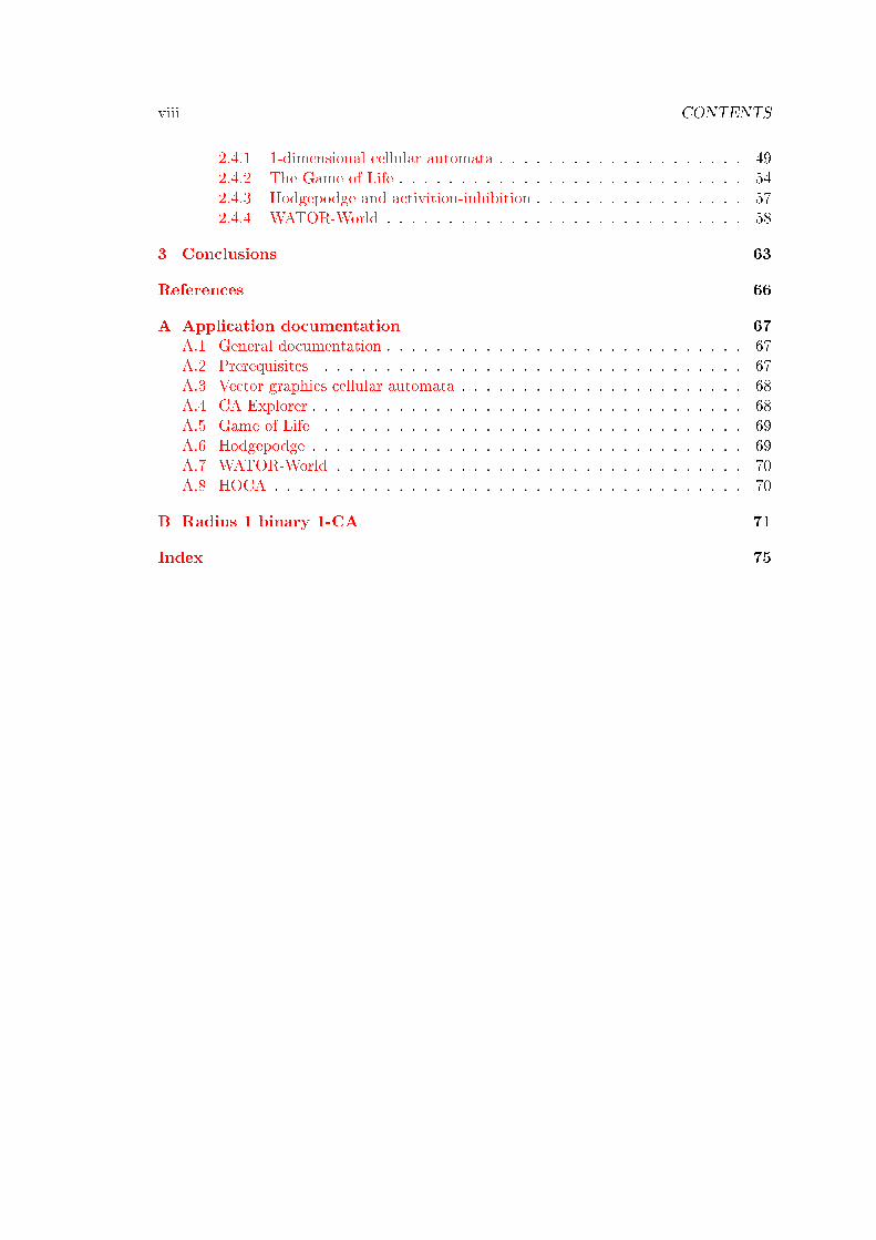
Figure 1.27: The hodgepodge machine after 1200 steps for various parameter combina-tions. The initial conguration is identical for all simulations with the same parameterg, so any dierence between the patterns is only due to the dierence in parameters.The row and column headers may be hard to read, so to clarify; along the x axis theparameter k1 has the values 0.5, 1, 1.5, 2, 3, 5, 8 and 12, and along the y axis k2 takeson the values 0.5, 1, 2, 4 and 6. These values were selected by trial and error so as toshow as many dierent behaviours as possible.

36 CHAPTER 1. CELLULAR AUTOMATA
Figure 1.28: Some of the other patterns that the hodgepodge machine may produce.

1.4. EXAMPLES 37
1.4.6 WATOR-World
Cellular Automaton 6 A predator-prey simulation CA
Lattice: L = Z× Z or Zn × ZmAlphabet: S = Z3 × Zmax(bf ,bs)+1 × Zs+1 × Z2
Neighbourhood: N = NvN (2-dimensional von Neumann)LTF: fw : S5 −→ S5 (asynchronous, algorithmic)
The following CA was proposed by Alexander Keewatin Dewdney in an article inScientic American [16, p. 154]. It is called WATOR-World, and is a discretizationof the Lotka-Volterra dierential equations, which model the relationship between thepopulations of a predator and its prey. Since such relationships are discrete in nature, aCA model will probably yield more realistic answers than dierential equations, all otherthings being equal. At the very least, it will solve the so-called atto-fox problem of [12,p. 32].25
In this CA, each cell is either empty water, a small sh, or a shark. The sharks andthe sh swim randomly about, and if a shark comes across a sh, the shark eats the sh.Both sh and sharks may reproduce once they reach a certain age. They breed by simplydepositing an ospring in the cell they leave a mate is not needed. At the same time,their age is reset, so as to avoid adult sh leaving behind a continuous trail of ospring.Finally, sharks will die if they go too long without food.
Stretching the CA denitions
This CA necessitates stretching the denitions of a CA a bit. Schi introduces this modelas a CA in [16], but later states that it is in fact an IBM, or individual-based model.An IBM focuses on the individuals that make up the model, instead of the locationsthat they occupy, as we do in cellular automata. Where we would iterate over the entirelattice, an IBM typically iterates over its population.
In forcing this into the CA framework, we get a problem because the subjects (shand sharks) often wander in a random direction. The obvious way of doing this in aCA is by swapping the states of two cells, where one is a sh and the other is its emptydestination. Though doable, such procedures must be considered carefully in a CA,because both the cells involved in the swapping must be in agreement that it is takingplace. If they are not, the result is a cloned sh, or a sh that has disappeared.
The fact that the direction of the swapping is random makes it much worse, if notimpossible, to implement as a standard CA. Take for example a seemingly simple prob-lem, will a sh leave its cell or not, depicted in gure 1.29. As can be seen, at the veryleast we'll need a bigger neighbourhood, and even then it is not so simple. If the nextmovements of the other four sh are not known, the sh in the middle may have a freecell to move to, or it may not.
25An atto-fox is 1 · 10−18 of a fox, which is the number of foxes per square kilometer that allowed thepopulation to rebound in the in the cited article.

38 CHAPTER 1. CELLULAR AUTOMATA
Will the fish leave the cell?
It might notbe able to.
Figure 1.29: One of the problems faced when implementing WATOR-World as a properCA.
The solution is to enable the LTF to change the state of neighbouring cells as wellas its own, and do the update in-place, or asynchronously. This means that the LTFwill decide the new position of a swimming entity based on where the sh around it arenow, as opposed to where they were one time step ago. We still keep the concept of atime step by denoting an update of every cell in the lattice as one time step.
There is also the problem that a sh might be moved several times in one time stepif it moves into an as of yet not updated cell. This we will mitigate by marking the shas moved, and making sure not to move sh that has been marked as moved already.
The algorithm
Let a : L −→ Z3 × Zmax(bf ,bs)+1 × Zs+1 × Z2 denote the global conguration map. Wedenote the state of an arbitrary cell by (w, a, l,m), where w is the presence of water (0),sh (1) or shark (2), a is the number of time steps since the sh or shark was born, lis the number of time steps since the last meal of a shark, and m is the ag indicatingthat the sh or shark has been moved. Further, let πw, πa, πl and πm be the projectionsfrom the alphabet S to each of the smaller sets. For example, πw((w, a, l,m)) = w, andsimilarly for a, l and m. Finally, the parameters of the CA are these: the breeding ageof sh and sharks we denote by bf and bs, respectively, and sharks starve after s timesteps without food.
Now lets specify the algorithm in detail. Because of the vagueness of the descriptionin [16], some details have been lled in or claried as the author saw t.
Each time step consists of two passes over the cells. The rst pass resets the value mto 0 for all the cells in the lattice, indicating that no sh has moved yet. The second passis done in random order while still making sure only to update each cell once. This is toavoid the tendency of tight packs of sh to move towards the starting point of the pass.Using the von Neumann neighbourhood NvN = ~n0, ~n1, ~n2, ~n3, ~n4 we do the followingfor each ~z ∈ L,
1. Denote the current state of the cell by (w, a, l,m).
2. If w = 0, do nothing more for this cell.
3. If w = 1 and m = 0, then:
a) If a ≤ bf , then increase a by one, aging the sh.

1.4. EXAMPLES 39
b) Let D = ~n ∈ NvN | πw(a(~z + ~n)) = 0.c) If D = ∅, the sh has nowhere to move, so update the state of the cell with
the new age by setting a(~z) = (1, a, 0, 1), and do nothing more for this cell.
d) If D 6= ∅, then pick a ~nx ∈ D at random.
e) If a = bf then the sh will breed, so we set a(~z + ~nx) = (1, 0, 0, 1) anda(~z) = (1, 0, 0, 1).
f) If a < bf , the sh simply moves, so we set a(~z + ~nx) = (1, a, 0, 1) and a(~z) =(0, 0, 0, 1).
4. If w = 2 and m = 0, then:
a) If a ≤ bs, then increase a by one, aging the shark.
b) If l = s, then the shark dies from hunger, so set a(~z) = (0, 0, 0, 0), and donothing more for this cell.
c) If l < s, then increase l by one, making the shark hungrier.
d) Let D = ~n ∈ NvN | πw(a(~z + ~n)) = 1.e) If D 6= ∅, then pick a ~nx ∈ D at random, and set l = 0, since the shark will
eat the sh at ~z + ~nx.
f) If D = ∅, then let D = ~n ∈ NvN | πw(a(~z + ~n)) = 0 instead.g) If D = ∅ even now, the shark has nowhere to move (very unlikely), update
the state of the cell with the new age and hunger by setting a(~z) = (2, a, l, 1),and do nothing more for this cell.
h) If l 6= 0, pick a ~nx ∈ D at random.
i) If a = bf then the shark will breed, so we set a(~z + ~nx) = (2, 0, l, 1) anda(~z) = (2, 0, 0, 1). The baby shark is born with a full stomach.
j) If a < bf , the shark simply moves, so set a(~z + ~nx) = (2, a, l, 1) and a(~z) =(0, 0, 0, 0).
Schi introduces two more parameters, nf and ns, the starting number of sh andsharks, respectively. A typical evolution of the WATOR world is pictured in gure 1.30.The sharks eat almost all the sh, and after a while great numbers starve to death sincemost of them nd no more food. A small remnant of sh sustain an even smaller numberof sharks, and for a while the sh breed faster than the sharks can eat. Soon the shhave multiplied to cover almost the whole lattice, while the sharks are becoming morenumerous again, feasting on the sh. All of a sudden, the sharks have eaten almost allthe sh, and the loop repeats, as shown in gure 1.31.
In this example we will study just one set of arbitrarily chosen parameters, namelybf = 8, bs = 20 and s = 20. We will consider the inuence the lattice size has on theway the CA behaves. The parameters nf and ns vary according to the size of the lattice,and to a small extent between simulations, but the sh
water and sharksh proportions will be
very similar for all the simulations.

40 CHAPTER 1. CELLULAR AUTOMATA
(a) t=1 (b) t=50 (c) t=80 (d) t=110 (e) t=150
(f) t=200 (g) t=260 (h) t=330 (i) t=410 (j) t=500
Figure 1.30: A WATOR-World evolution on an 120x90 lattice with bf = 8, bs = 20 ands = 20. Black cells are sharks, gray cells are sh and white cells are water. To constructthe initial conguration, 20% of the lattice cell states were set to state (1,0,0,0), then15% were set to state (2,0,0,0), possibly overwriting some of the previously set values.
0
2000
4000
6000
8000
10000
12000
0 200 400 600 800 1000 1200 1400 1600 1800 2000
Count
Time step
FishShark
Figure 1.31: A graph showing the population of sh and sharks. This graphs the datafrom the simulation shown in gure 1.30. The graph lines are saw-toothed because theindividuals all tend to breed simultaneously; sh every 8th time step and sharks every20th. The sh curve gets smoother as time progresses because sh trapped on all sideswill delay breeding until there's room enough, thereby also delaying the breeding schedulefor all descendants. Sharks almost always have room to breed.
The results are graphed in gure 1.32, and as we can see, there is a gradual changehappening between the smallest lattice size and the largest. In the smallest, only one often simulations had any shark alive after 100 steps. In the largest, only one of ten didn't,and only one more didn't make it to the end of the simulation at 1000 steps.

1.4. EXAMPLES 41
It might be tempting to conclude from this data that threatened species that havea predator-prey relationship need large natural reserves for them to have any chance ofsurviving. However, while there may be some truth to this thinking, the model is far toocoarse for us to apply the results obtained through it to the real world. Here are someways in witch we could have improved on it, and as the attentive reader will realize, someof them would probably have helped the sharks in the small lattice survive in the longrun:
• Get actual data for breeding ages of both species.
• Also get data for how long a predator can live without prey.
• Take into account that time to rst breeding and time to consequent breedingsmight not be the same.
• Give the predators a nite stomach size.
• Have the individuals die of old age at some point.
• Factor in how the prey might hide from or successfully escape the predator.
• Have the prey gather in groups, as they often do in nature, to protect themselvesfrom predators.
• Factor in the inuence of seasons.
• Add additional types of prey that the predator might catch and eat if it is hungryenough, or seasonal prey that sometimes ease the preassure o of the primary prey.
• Add additional types of predators or omnivores that may target the same type ofprey as the main predator.
• Have some upper bound on the number of prey, as they will not grow totallywithout bound in nature.
• Give the predators some sense of smell or sight so they may target prey and moveabout more purposefully.
We will come back to the last point of this list in section 2.4.4.

42 CHAPTER 1. CELLULAR AUTOMATA
0
100
200
300
400
500
600
700
800
900
0 50 100 150 200 250 300
Count
Time step
FishShark
(a) Z30 × Z30
0
500
1000
1500
2000
2500
3000
3500
4000
0 100 200 300 400 500 600 700 800 900
Count
Time step
FishShark
(b) Z60 × Z60
0
1000
2000
3000
4000
5000
6000
7000
8000
0 100 200 300 400 500 600 700 800 900 1000
Count
Time step
FishShark
(c) Z90 × Z90
0
2000
4000
6000
8000
10000
12000
14000
16000
0 100 200 300 400 500 600 700 800 900 1000
Count
Time step
FishShark
(d) Z120 × Z120
Figure 1.32: 10 runs of four dierent lattice sizes. The parameters and initial congura-tions are as described in the caption of gure 1.30

Chapter 2
Higher Order Cellular Automata
2.1 Introduction
In section 1.4.2 we created a very complicated radius 1 generic CA from a simple radius4 totalistic CA, and observed that the simple rule produced a pattern much better suitedfor human eyes than the complicated equivalent. The logical connections of the advancedrule were hidden from human eyes. It is natural then to consider how we can put a greaternumber of the very many complicated CAs1 into equivalent simple CAs that are easierto study and understand. To do that we need to extend the concept of a CA, but do soin a way that is structured easily reduced into its component pieces, so that the wholething can be picked apart and studied.
According to [3], Torbjørn Helvik introduced the concept of higher order cellularautomata [9], abbreviated HOCA, in 2001. He based it on the concept of hyperstructuresintroduced by Nils A. Baas in [1] in 1994. In brief, a HOCA is a CA with additionaldynamics and/or hierarchical structure. With this framework it is possible for instance tocombine several dierent normal CAs into one, or to make groups of cells that inuenceeach other in some way, independent of the local transition function.
We will see that this enables us to design (randomly or with purpose) and understandCAs whose explicit form LTF would have been close to undecipherable. It uncovers atreasure trove of very interesting and unexpected behaviour, and gives us tools we mayuse to study simple CAs. Finally, we may use HOCAs to meaningfully alter the behaviourof existing CAs to suit our needs.
1What we mean here by complicated CA is a CA with a large number of states and/or a largeneighbourhood, and a LTF that seems only to be expressible as a lookup table; that is, there seems tobe no formula or algorithm that does the same job. These kinds of CA are naturally extremely plentiful,and a small subset of them probably do some very neat things.
43

44 CHAPTER 2. HIGHER ORDER CELLULAR AUTOMATA
2.2 Denition
In this section we will use the denitions of [2] with some small changes in notation. Westart with giving some already dened symbols a little subscripted number: Let L1 bea lattice, S1 be an alphabet and a1 : L1 −→ S1 be the state conguration of L1. Inall these symbols, the subscript 1 refers to the rst morphological level of the HOCA.A morphological level is what we call each oor of the hierarchical structure of theHOCA. We may drop the subscript if there is only one such morphological level.
2.2.1 2-dynamics
In a normal cellular automaton, every cell of the lattice has the same neighbourhood andthe same local transition function. Higher order cellular automata with 2-dynamics mayassign dierent neighbourhoods and LTFs to each cell. We now introduce the necessaryconcepts to deal with this.
Let N1 = N1, N2, . . . , Nk denote the set of all the possible neighbourhoods that acell might have. Then we may dene a map that maps each cell to the neighbourhood ituses, n1 : L1 −→ N1. The function n1 is called the rst level neighbourhood conguration,and the set N1 is the rst level 2-neighbourhood.
Now we must assign one local transition function to each cell. However, the LTF ofeach cell must be compatible with the neighbourhood of that cell, meaning that if acell has the neighbourhood Nx, then the LTF of that cell must have S|Nx| as domain. Tofacilitate this, we dene a set
M = |N | | N ∈ N1
In words, M is the set of the dierent cardinalities that all the possible neighbourhoodshave. We now dene the rst level 2-rule R1 = f1, f2, . . . , fk as a set of local transitionfunctions such that
1. Each function is of the form fi : Sm1 −→ S1 for some m ∈M .
2. For each m ∈M there is at least one function fj ∈ R with domain Sm1 .
This lets us divide the sets R1 and N1 into disjoint subsets according to the cardinalityof the neighbourhood:
Rm1 = f ∈ R1 | f : Sm1 −→ S1Nm
1 = N ∈ N1 | |N | = m
Now we may nally dene the function r1 : L1 −→ R1 that maps one local tranistionfunction to each cell. It must be such that
r1(~z) ∈ Rm1 if and only if n1(~z) ∈ Nm1 for all ~z ∈ L1

2.2. DEFINITION 45
To introduce the 2-dynamics, we need a function φ1 that updates the functions n1
and r1 each time step, in the same way that a1 is updated by the LTF each time stepin a regular cellular automaton. To put into mathematical notation the restriction thatthe functions n1 and r1 must always be compatible, we rst dene the target set Φ1 ofthis function:
Φ1 = (N, f) ∈ N1 ×R1 | (N, f) ∈ Nm1 ×Rm1 for some m ∈M
For each m ∈M we dene a function
φm1 : Sm1 ×Nm1 ×Rm1 −→ Φ1
These functions may then be combined to form the 2-transition map φ1 = (φm1 )m∈M .
2.2.2 2-morphology
We now go on to group the cells of the lattice L1 into 2-cells or organs. To achieve thiswe dene the second order lattice, L2, and a map M : L2 −→ P(L1). For an arbitraryorgan, let's say it is at ~z ∈ L2, the set M(~z) contains the coordinates of the cells in L1
that are contained in that organ. We also dene the reciprocal map M∗ : L1 −→ P(L2),such that for an arbitrary cell ~z ∈ L1, M
∗(~z) is the set of organs2 that contain the cellat ~z:
M∗(~z) = ~x ∈ L2 | ~z ∈M(~x)
Each 2-cell has a single state, and the set of all possible states is the second levelalphabet S2. The state of each 2-cell is given by the second level state congurationa2 : L2 −→ S2. Now we might alter the domain of the 2-transition map so that the stateof the 2-cells may inuence it:
φm1 : Sm1 × S2 ×Nm1 ×Rm1 −→ Φ1
Similarly we might make the rules in the 2-rule of the rst level also take S2 as aninput3. At this point we may choose to do one of three things:
• We may dene a function f2 : SC1 −→ S2, where SC1 is some kind of aggregate
value of the 1-cells in the organ4. This means that we're using the 2-cell only as astorage mechanism for some aggregate information, which then inuences the rstlevel rule and 2-transition map one time step later.
2This means, of course, that a cell may be in several organs at once.3If the same 1-cell may be in several 2-cells, we need to alter the functions slightly to take that into
account. Exactly how this is done will vary from problem to problem, depending on what the HOCAshould model or what its desired behaviour is.
4The set SC1 need not be equal to the set S1; it could be a subset of Z and be the result of a sum, or
a binary value inticating the presence or absence of some condition, or the product space of several suchindicators.
46 CHAPTER 2. HIGHER ORDER CELLULAR AUTOMATA
• We may dene a single second level neighbourhood N2 and a local transition func-
tion f2 : S|N2|2 × SC1 −→ S2, giving dynamics to the second level.
• Lastly, we may bestow 2-dynamics on the second level as well, by dening
a second level 2-neighbourhood N2,
a second level neighbourhood conguration n2 : L2 −→ N2,
a second level 2-rule R2,
a second level rule conguration r2 : L2 −→ R2, and
second level 2-transition maps φm2 : Sm2 × SC1 ×Nm2 ×Rm2 −→ Φ2.
How to build additional levels should now be evident. If we get as far as adding3-cells to the model, we may of course modify the second level rules and 2-transitionmap to depend on the state of the 3-cells that the 2-cells belong to, just like we did withthe rules and 2-transition map on the rst level after adding the 2-cells.
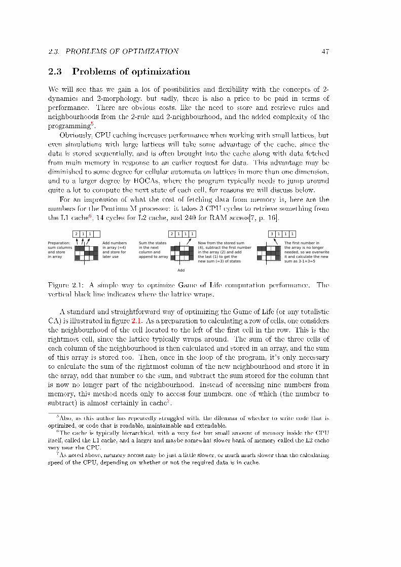
2.3. PROBLEMS OF OPTIMIZATION 47
2.3 Problems of optimization
We will see that we gain a lot of possibilities and exibility with the concepts of 2-dynamics and 2-morphology, but sadly, there is also a price to be paid in terms ofperformance. There are obvious costs, like the need to store and retrieve rules andneighbourhoods from the 2-rule and 2-neighbourhood, and the added complexity of theprogramming5.
Obviously, CPU caching increases performance when working with small lattices, buteven simulations with large lattices will take some advantage of the cache, since thedata is stored sequentially, and is often brought into the cache along with data fetchedfrom main memory in response to an earlier request for data. This advantage may bediminished to some degree for cellular automata on lattices in more than one dimension,and to a larger degree by HOCAs, where the program typically needs to jump aroundquite a lot to compute the next state of each cell, for reasons we will discuss below.
For an impression of what the cost of fetching data from memory is, here are thenumbers for the Pentium M processor: it takes 3 CPU cycles to retrieve something fromthe L1 cache6, 14 cycles for L2 cache, and 240 for RAM access[7, p. 16].
Preparation:sum columnsand storein array
Add
Now from the stored sum (4), subtract the first numberin the array (2) and add the last (1) to get the new sum (=3) of states
The first number inthe array is no longerneeded, so we overwriteit and calculate the newsum as 3-1+3=5
2 1 1
Add numbersin array (=4)and store for later use
2 1 1 1
Sum the statesin the nextcolumn andappend to array
3 1 1 1
Figure 2.1: A simple way to optimize Game of Life computation performance. Thevertical black line indicates where the lattice wraps.
A standard and straightforward way of optimizing the Game of Life (or any totalisticCA) is illustrated in gure 2.1. As a preparation to calculating a row of cells, one considersthe neighbourhood of the cell located to the left of the rst cell in the row. This is therightmost cell, since the lattice typically wraps around. The sum of the three cells ofeach column of the neighbourhood is then calculated and stored in an array, and the sumof this array is stored too. Then, once in the loop of the program, it's only necessaryto calculate the sum of the rightmost column of the new neighbourhood and store it inthe array, add that number to the sum, and subtract the sum stored for the column thatis now no longer part of the neighbourhood. Instead of accessing nine numbers frommemory, this method needs only to access four numbers, one of which (the number tosubtract) is almost certainly in cache7.
5Also, as this author has repeatedly struggled with, the dilemma of whether to write code that isoptimized, or code that is readable, maintainable and extendable.
6The cache is typically hierarchical, with a very fast but small amount of memory inside the CPUitself, called the L1 cache, and a larger and maybe somewhat slower bank of memory called the L2 cachevery near the CPU.
7As noted above, memory access may be just a little slower, or much much slower than the calculatingspeed of the CPU, depending on whether or not the required data is in cache.

48 CHAPTER 2. HIGHER ORDER CELLULAR AUTOMATA
For HOCAs with more than one possible neighbourhood, this optimization techniquecannot easily be used. For totalistic HOCAs, the rule function8 would presumablycall a sum member function belonging to the neighbourhood object or the lattice
object, which would then calculate the sum from scratch and return it. Not only doesthis remove the ability to implement the above optimization technique, it also incursthe added overhead of a function call, which for some programming languages can beconsiderable.
A more advanced optimization technique applicable to many types of cellular au-tomata was introduced by William Gosper in a 1984 article [8]. This technique hasbecome known as hashlife when used to optimize the Game of Life. It stores the cellstates9 in a tree representation called a quadtree, rather than in a matrix, to allow thelattice to expand as much as needed to t the pattern of non-quiescent cells. This hasthe added advantage that it can be combined with hashing to canonicalize the contents,meaning every occuring state pattern needs only be stored once, and this pattern is thenjust pointed to whenever it occurs in the lattice. Lastly memoization is used, whichmeans that the function computing the next time step of a part of the tree, stores theresults for later use10.
Hashlife, properly implemented and optimized, can speed up the simulation by sev-eral orders of magnitude, and enable the simulation of huge lattices of Game of Life fortrillions of generations as they grow to billions of cells [14]. Of course, the design ofthis algorithm hinges on a couple of assumptions: The underlying CA must be determin-istic, or else memoization could not be used. The set of commonly occuring sub-patternsmust be small enough to t in memory, so that canonicalization actually gives an ad-vantage. CAs without these properties would probably fare worse if implemented withGospers algorithm rather than the naive one, since they would get the added overheadfor canonicalization and memoization without reaping the benets.
If one wished to implement a HOCA using this algorithm, the state of a cell, whenviewed from the perspecive of the algorithm, would need to include not only the state ofthe cell, but also its rule, its neighbourhood, and the states, rules and neighbourhoodsof all its organs. This would of course dramatically increase the number of possible sub-patterns that the algorithm would need to cope with. For all but the most simple HOCAsthen, this would make both canonicalization and memoization impractical, rendering alsothis optimization technique moot.
In summary, giving a cellular automaton 2-morphology or 2-dynamics may slow thecomputation down to a much larger degree than the extra necessary computation shouldwarrant, making the study of large-scale HOCAs, be it in space or time, impractical,time-consuming or expensive.
8Here we are using the word function to refer to the programming construct, rather than themathematical notion.
9More precisely: the states of the cells which are in the support of the conguration.10Garbage collection is also needed to prune infrequently needed results from the stored results, thereby
avoiding running out of memory.

2.4. EXAMPLES 49
2.4 Examples
2.4.1 1-dimensional cellular automata
We start out by looking at a simple variation of the rst example given in Baas andHelvik[2], where instead of totalistic rules, we use the kind of rules presented in section1.4.1. As an overview then, we have the following system:
Cellular Automaton 7 Radius 1 binary 1-HOCA with 2-dynamics
Lattice: L = Z or ZnAlphabet: S = Z2
2-neighbourhood: N = −1, 0,−1 (rst neighbours)2-rule: R = fa, fb (fa and fb as in section 1.4.1)
2-transition map: φ : S3 ×R −→ R (totalistic)
The 2-transition map has two parameters, ca and cb, and depends on the sum s ∈ Z4
of the states of the cells in the neighbourhood, and the current rule f ∈ R:
φ(s, f) =
fa if f = fb and s = cbfb if f = fa and s = caf otherwise
This simple HOCA enables much more complex behaviour than its constituent partsmight suggest. As an example, let fa be rule 255 and fb rule 28. Rule 255 sets the cellstate to 1 no matter the input, so it is natural to assume that the combined HOCA wouldbehave somewhat similar to rule 28, since rule 255 seems not to add anything. But aswe can see in gure 2.2, this is not the case.
Figure 2.2: A combination of rule 255 and rule 28 where ca = 3 and cb = 2. Examplesof how the two rules look by themselves are to the left, while the HOCA that is thecombination as described above is in the rightmost frame. Since there is now also apattern formed by which rule is applied in each cell, the type of pattern (State or Rule)is now specied under each pattern. Then the parameters for the HOCA as a whole isspecied beneath. All cells have a random state and (where applicable) rule as initialconguration. Black is 1 and white is 0 for the state patterns, and black is fb and whiteis fa in the rule pattern.
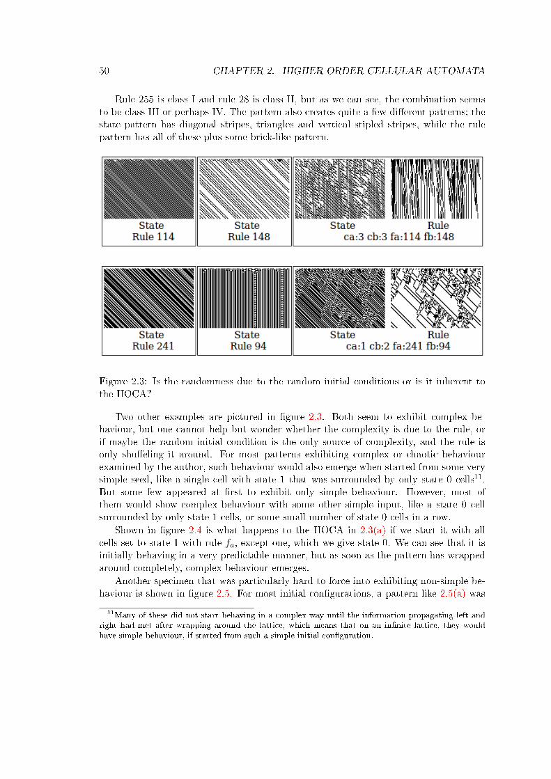
50 CHAPTER 2. HIGHER ORDER CELLULAR AUTOMATA
Rule 255 is class I and rule 28 is class II, but as we can see, the combination seemsto be class III or perhaps IV. The pattern also creates quite a few dierent patterns; thestate pattern has diagonal stripes, triangles and vertical stipled stripes, while the rulepattern has all of these plus some brick-like pattern.
Figure 2.3: Is the randomness due to the random initial conditions or is it inherent tothe HOCA?
Two other examples are pictured in gure 2.3. Both seem to exhibit complex be-haviour, but one cannot help but wonder whether the complexity is due to the rule, orif maybe the random initial condition is the only source of complexity, and the rule isonly shueling it around. For most patterns exhibiting complex or chaotic behaviourexamined by the author, such behaviour would also emerge when started from some verysimple seed, like a single cell with state 1 that was surrounded by only state 0 cells11.But some few appeared at rst to exhibit only simple behaviour. However, most ofthem would show complex behaviour with some other simple input, like a state 0 cellsurrounded by only state 1 cells, or some small number of state 0 cells in a row.
Shown in gure 2.4 is what happens to the HOCA in 2.3(a) if we start it with allcells set to state 1 with rule fa, except one, which we give state 0. We can see that it isinitially behaving in a very predictable manner, but as soon as the pattern has wrappedaround completely, complex behaviour emerges.
Another specimen that was particularly hard to force into exhibiting non-simple be-haviour is shown in gure 2.5. For most initial congurations, a pattern like 2.5(a) was
11Many of these did not start behaving in a complex way until the information propagating left andright had met after wrapping around the lattice, which means that on an innite lattice, they wouldhave simple behaviour, if started from such a simple initial conguration.

2.4. EXAMPLES 51
Figure 2.4: Complex behaviour arising because of a wrapping lattice.
the result, and such patterns stay predictable even on nite wrapping lattices. But forcertain special initial congurations, some very dierent patterns would emerge, and forsome, it even depended on the width of the lattice, as is appearant from gure 2.5(b)and 2.5(c). It is hard to believe that all these patterns could have been made by thesame CA.
The HOCA in this example can also be used to extract or highlight patterns createdby any other CA, by setting fa = fb. Now the pattern created will not be inuencedat all by which rule is used, since they're both the same, but the rule pattern will showa pattern based on the evolution of the neighbourhood conguration of each cell. Someexamples are shown in gure 2.6.
This HOCA has been a suprisingly rich source of dierent behaviours, and might beworth further study.

52 CHAPTER 2. HIGHER ORDER CELLULAR AUTOMATA
Figure 2.5: Complex behaviour arising out of simple initial conditions. All the images areof the same HOCA with fa = 241, fb = 94, ca = 1, cb = 2. Each image subtext speciesthe pattern of initial states with which the initial conguration was made, placed in thecenter of a lattice that has state 1 (black) elsewhere. The number in paranthesis is thewidth of the lattice. The rule is initially set to fa for all cells.
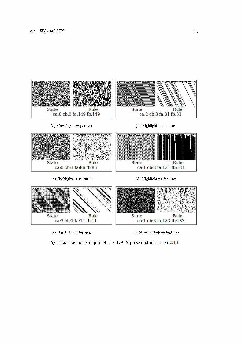
2.4. EXAMPLES 53
(a) Creating new pattern (b) Highlighting features
(c) Highlighting features (d) Highlighting features
(e) Highlighting features (f) Showing hidden features
Figure 2.6: Some examples of the HOCA presented in section 2.4.1

54 CHAPTER 2. HIGHER ORDER CELLULAR AUTOMATA
2.4.2 The Game of Life
With a general HOCA framework implemented it is rather easy to change an existingCA in some way. The following example shows how adding very simple 2-dynamics tothe Game of Life will change its long-term behaviour, while still keeping it deterministicand behaving mostly as before on a short time scale.
When starting the standard Game of Life from a random initial conguration, thereis at rst very much activity, but soon much of it dies down and settles into blinkers orstill life. It is inevitable that some activity starting somewhere else on the lattice crashesinto these xtures during its evolution, which of course causes it to behave dierentlythan it would have, had the unmoving life not been there. What if we could removethe clutter if it was left alone for some time, so that the moving patterns could unfoldnaturally? We can use 2-dynamics to do this.
Cellular Automaton 8 Binary outer totalistic 2-CA
Lattice: L = Z× Z or Zn × ZmAlphabet: S = Z2
2-Neighbourhood: N = NM (2-dimensional Moore neighbourhood)2-Rule: R = f0, f1, . . . , fk, fk+1, . . . , fk+lLTFs: fi = g h : S9 −→ Z9 × Z2 −→ S for i < k
fi : S9 −→ 0 for k ≤ i ≤ k + l2-Transition map: φ : S9 ×R −→ R
All the fi LTFs for i ∈ 0, 1, . . . , k−1 are the normal Game of Life LTF, completelyunchanged. The rest of the fi functions are, as is obvious from their codomain, thenull function. The 2-transition map depends on the states of the cells in the Mooreneighbourhood and the current rule. We reuse the function f from section 1.4.4 to denethe 2-transition map:
φ(s0, s1, . . . , s8, fi) =
fi+1 if i < k and f(s0, s1, . . . , s8) = s0 and s0 = 1fi+1 if k ≤ i < k + lf0 otherwise.
So for a total of k−1 time steps, a cell that remains unchanged and alive will behaveas in the normal game of life. But then in the kth time step, such a longlived cell willsuddenly become dead, and remain dead no matter what happens around it for a furtherl time steps12. After that, it will behave normally again. If the long-lived cell dies bynormal means before k time steps have passed, it will start from scratch again and usef0 as its local transition function, so even if it immediately comes alive again and staysthat way, it will have another k− 1 time steps before it's killed o by our null functions.
12This is to kill o the very stable 2 × 2 squares that are so common they will rebound if just onecell is killed at a time, so we need to wait until more than 2 are dead to actually remove such patternsfrom the lattice.

2.4. EXAMPLES 55
It's quite straightforward to implement this HOCA as a standard CA by changingthe alphabet to something like S = Z2 × Zk+l and changing the LTF to also count thenumber time steps a cell has been alive. However, any CA with only 2-dynamics and not2-morphology is conjugate to an ordinary CA this is just a case that can very easily beseen as such. [2]
10
100
1000
10000
100000
0 1000 2000 3000 4000 5000 6000 7000
Count
Time step
Changes CAChanges HOCA
1
10
100
1000
10000
100000
0 500 1000 1500 2000 2500 3000 3500 4000 4500
Count
Time step
Changes CAChanges HOCA
Figure 2.7: A couple of simulations with the same initial conguration for the traditionalGame of Life CA and our HOCA variant. Both gures show a simulation on a Z200×Z200
lattice. The initial conguration is constructed by setting the state of each cell to alivewith 30% probability, and otherwise dead.
To study what eect the 2-dynamics has on the CA, we run the CA and the HOCAsimultanously with the same initial conguration, and for each time step, we count thenumber of cells that change from alive to dead or from dead to alive, and plot this numbervs. time. The results of two such simulations are shown in the subgures of gure 2.7.The HOCA always seems to end up with just some small number of gliders, while the CAstabilizes into the usual clutter of still life and blinkers a glider would soon collide withthe clutter, so there are no gliders left when the CA stabilizes. We haven't got enoughinformation to draw any conclusions yet we need more data.
So instead of plotting the number of changes vs. time, we make a note of the timestep at which the number of changes stabilized for both the CA and its equivalent HOCA.Then we plot this data as in gure 2.8.
Here we see a denite tendency, which is that the HOCA will stabilize sooner thanits equivalent CA. So the still life and blinkers are actually not preventing the movinglife from living, but helping it stay moving for a longer period than it would otherwisehave done.

56 CHAPTER 2. HIGHER ORDER CELLULAR AUTOMATA
0
1000
2000
3000
4000
5000
6000
7000
0 1000 2000 3000 4000 5000 6000 7000 8000
HO
CA
tim
e s
teps
CA time steps
Figure 2.8: The time to stabilization for a Game of Life CA vs. its HOCA equivalentwith the same initial conguration. The lattice and initial conguration are as describedin gure 2.7.
2.4. EXAMPLES 57
2.4.3 Hodgepodge and activition-inhibition
The author has not managed to think of any ways these two CAs can meaningfully begiven 2-dynamics or 2-morphology without breaking away from the purpose the CA wasdesigned for. The hodgepodge machine was made to simulate a chemical reaction, andit does that job well. There are no hierarchies involved in the reaction, and using thesame rule and neighbourhood for all cells is sucient, more dynamics is not needed.
The activition-inhibition model was also made for a spesic purpose which it fulllsnicely; to reproduce patterns found on snail shells. These patterns are produced by rowsof glands around the base of the snail as they secrete the shell itself. The existing modelobviously does a good job of it, and there are no obvious hierarchical structures we mayadd here either.
We therefore move on to the last example, which is much better suited for higherorder extensions.

58 CHAPTER 2. HIGHER ORDER CELLULAR AUTOMATA
2.4.4 WATOR-World
Sharks are known for their excellent sense of smell, especially when it comes to blood,and they use this to nd places nearby where other sharks have found food. We willadd this behaviour to our WATOR-World CA by adding 2-morphology and altering thealgorithm from section 1.4.6.
Cellular Automaton 9 A predator-prey simulation HOCA
Lattices: L1 = Z× Z or Z3n × Z3m
L2 = Z× Z or Zn × ZmAlphabets: S1 = Z3 × Zmax(bf ,bs)+1 × Zs+1 × Z2 × Z2
S2 = Z9900 ×NvN
2-Neighbourhoods: N1 = NvN (rst neighbours)N2 = NvN (rst neighbours)
2-rules: R1 = fwR2 = fd
Local Transition Functions: fw : S51 × S2 −→ S5
1 (asynchronous, algorithmic)fd : S5
2 × SC1 −→ S2 (algorithmic)
We have appended ×Z2 to the alphabet of the rst level to serve as the indicator ofblood having been spilt in a cell during that time step. We will denote the new state ofa 1-cell by (w, a, l,m, b), where the rst four are as before, while b is 1 if a sh was eatenin this cell this turn, and 0 if not.
As the rst level lattice is 3 times larger than the second level lattice, we will use thefunctions 2.1 and 2.2 to map each 2-cell to the 1-cells it contains and vice versa. In these
formulas,⌊
(x,y)3
⌋= (⌊y
3
⌋,⌊x3
⌋).
M(~z ∈ L2) = ~x ∈ L1 |⌊~x
3
⌋= ~z (2.1)
M∗(~x ∈ L1) =⌊~x
3
⌋(2.2)
The second level state is a two-tuple that we'll denote by (c, d), where c ∈ Z9900 isthe concentration of blood in the water of that cell13, and d ∈ NvN is the direction of thegreatest increase of blood concentration. We'll let πc and πd be the projections of thestate set down to its factors, so that πc((c, d)) = c and πd((c, d)) = d. The projectionsfrom section 1.4.6 we will alter so that they project from the new alphabet set, and wewill add a projection for the new b indicator, which will then be πb((w, a, l,m, b)) = b.
Now we are ready to list the modied rst level algorithm, which we've called fw.Unaltered portions are grayed out.
1. Denote the current state of the cell by (w, a, l,m, b).139900 is a coarse upper bound for the concentration of blood in the water that can be achieved with
the algorithm we'll use.

2.4. EXAMPLES 59
2. If w = 0, do nothing more for this cell.
3. If w = 1 and m = 0, then:
a) If a ≤ bf , then increase a by one, aging the sh.
b) Let D = ~n ∈ NvN | πw(a1(~z + ~n)) = 0.c) If D = ∅, the sh has nowhere to move, so update the state of the cell with
the new age by setting a1(~z) = (1, a, 0, 1, 0), and do nothing more for this cell.
d) If D 6= ∅, then pick a ~nx ∈ D at random.
e) If a = bf then the sh will breed, so we set a1(~z + ~nx) = (1, 0, 0, 1, 0) anda1(~z) = (1, 0, 0, 1, 0).
f) If a < bf , the sh simply moves, so we set a1(~z + ~nx) = (1, a, 0, 1, 0) anda1(~z) = (0, 0, 0, 1, 0).
4. If w = 2 and m = 0, then:
a) If a ≤ bs, then increase a by one, aging the shark.
b) If l = s, then the shark dies from hunger, so set a1(~z) = (0, 0, 0, 0, 0), and donothing more for this cell.
c) If l < s, then increase l by one, making the shark hungrier.
d) Let D = ~n ∈ NvN | πw(a1(~z + ~n)) = 1.e) If D 6= ∅, then pick a ~nx ∈ D at random, and set l = 0 and b = 1, since the
shark will eat the sh at ~z + ~nx.
f) If D = ∅, then let D = ~n ∈ NvN | πw(a1(~z+ ~n)) = 0 instead, and set b = 0,since the shark did not nd any food.
g) If D = ∅ even now, the shark has nowhere to move (very unlikely), update thestate of the cell with the new age and hunger by setting a1(~z) = (2, a, l, 1, b),and do nothing more for this cell.
h) If l 6= 0, then:
i) Let ~np = πd(a2(M∗(~z))).ii) If ~np ∈ D then let ~nx = ~np.
iii) If ~np /∈ D then let ~nx =[
0 −11 0
]~np.
14
iv) If ~nx /∈ D then let ~nx =[
0 1−1 0
]~np.
v) If ~nx /∈ D then let ~nx =[−1 0
0 −1
]~np.
i) If a = bf then the shark will breed, so we set a1(~z + ~nx) = (2, 0, l, 1, b) anda1(~z) = (2, 0, 0, 1, 0). The baby shark is born with a full stomach.
14This amounts to rotating the vector ~np in a counterclockwize direction. The next step then attemptsa clockwize rotation instead, and the last one is a 180 turn. Thus, when there is a denite gradient inthe 2-cell and no food around, the movement of the sharks is wholly deterministic.

60 CHAPTER 2. HIGHER ORDER CELLULAR AUTOMATA
j) If a < bf , the shark simply moves, so set a1(~z + ~nx) = (2, a, l, 1, b) anda1(~z) = (0, 0, 0, 0, 0).
To summarize the changes: we added a bloodspill indicator to a cell whenever a sharkeats a sh, and we made the shark swim in the direction of the gradient aquired fromthe 2-cell, if in could not nd food. If unable to swim in that direction, it would try togo around the obstackle.
The second level algorithm, which we've called fd is rather more straightforward.We'll dene the aggregate k(~z) ∈ SC1 of the 1-cells in each 2-cell as k(~z) =
∑~x∈M(~z) πb(a1(~x)).
Then we do the following for each ~z ∈ L2:
1. Let ~ng ∈ NvN be a vector such that πc(a2(~z+~ng)) > πc(a2(~z+~n)) for all ~n ∈ NvN
such that ~ng 6= ~n.
2. If no such vector exists, then let ~ng = (0, 0).
3. Let
c =∑
~n∈NvN
(πc(a2(~z + ~n))
1.1 · 5
)+ 100k(~z).
4. The next state of the 2-cell at ~z will be (c, ~ng).
What happens is that any shark killing a sh will cause a sharp increase of the bloodconcentration in the 2-cell containing that cell. After only one time step that concentra-tion will have diused completely across ve 2-cells, so if a 2-cell has a concentration of100 in time step 1, all cells in its von Neumann neighbourhood will have a concentrationof 20 at time step two, barring other sharks eating nearby. That is not quite the truthhowever, because we also divide by a decay factor of 1.1, so that the actual concentrationof all ve cells at time step two is 18.
Because of the decay factor, the smell of an old kill will not linger for very long, andthe concentration of blood in the water is bounded. A typical run of this new algorithmresults in quite dierent behaviour than the original algorithm, as is shown in gure 2.9and 2.10(a). What is more, the lattice size dependency that we noticed in section 1.4.6is now very much diminished, as gure 2.10(b) shows cleary when compared with gure1.32(a). The HOCA model reaches the 1000th time step all 10 times without the sharksdying out, compared with 0 times for the plain CA.
Whether this is a step in the right direction can be debated however. The populationgraphs of gure 2.10(b) no longer displays the characteristic predator-prey curves thatthe Lotka-Volterra model produces, which are known to occur in nature.
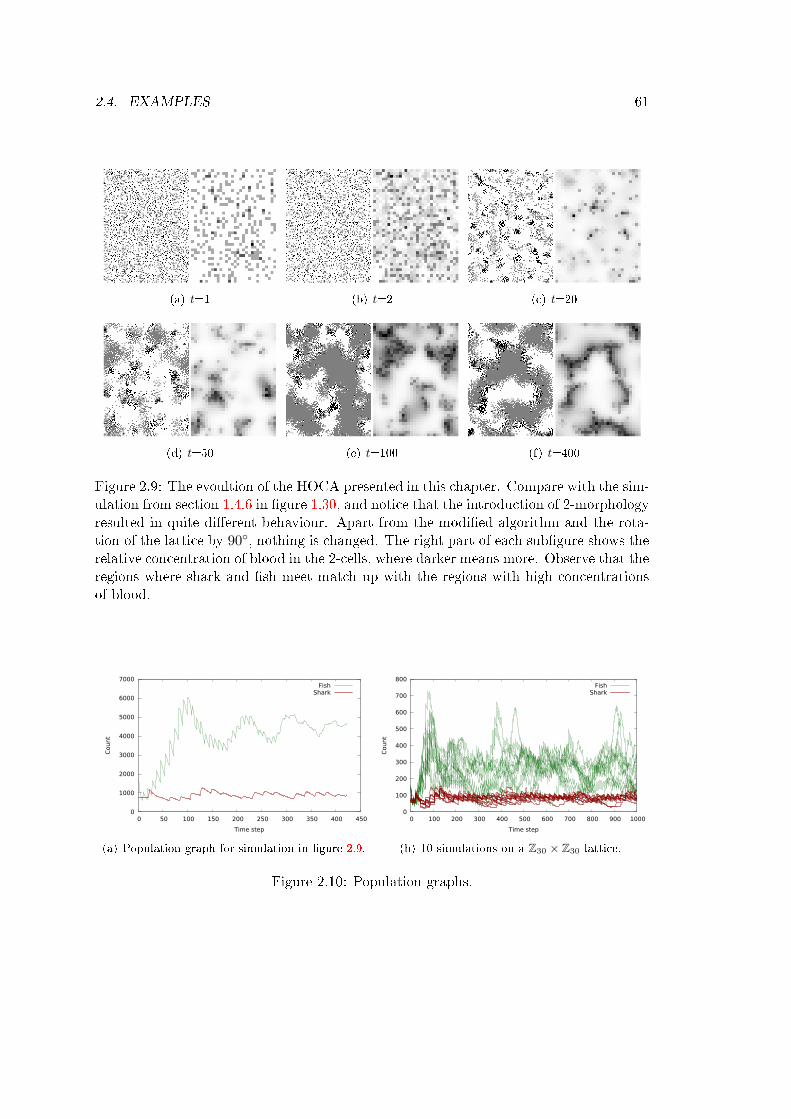
2.4. EXAMPLES 61
(a) t=1 (b) t=2 (c) t=20
(d) t=50 (e) t=100 (f) t=400
Figure 2.9: The evoultion of the HOCA presented in this chapter. Compare with the sim-ulation from section 1.4.6 in gure 1.30, and notice that the introduction of 2-morphologyresulted in quite dierent behaviour. Apart from the modied algorithm and the rota-tion of the lattice by 90, nothing is changed. The right part of each subgure shows therelative concentration of blood in the 2-cells, where darker means more. Observe that theregions where shark and sh meet match up with the regions with high concentrationsof blood.
0
1000
2000
3000
4000
5000
6000
7000
0 50 100 150 200 250 300 350 400 450
Count
Time step
FishShark
(a) Population graph for simulation in gure 2.9.
0
100
200
300
400
500
600
700
800
0 100 200 300 400 500 600 700 800 900 1000
Count
Time step
FishShark
(b) 10 simulations on a Z30 × Z30 lattice.
Figure 2.10: Population graphs.

62 CHAPTER 2. HIGHER ORDER CELLULAR AUTOMATA

Chapter 3
Conclusions
In this thesis we have given an introduction to the concepts of cellular automata andhigher order cellular automata. We have seen some examples of the widely dierent andsometimes unexpected patterns that cellular automata can produce.
Then we went on to introduce higher order cellular automata, and considered how,while giving a lot of advantages, they also slow the implementation down to some degreebecause the presumptions that various optimisation techniques rest upon are no longersatised.
We have observed how some cellular automata are in a sense complete, and givinghigher order structures or 2-dynamics to them seems unnatural. Other cellular autmoatavery naturally accept higher order structures, and can rather easily be extended to betterapproximate the real world phenomena the model is based upon to give better and moreaccurate answers.
63

64 CHAPTER 3. CONCLUSIONS

Bibliography
[1] Baas, N. A. [1994], Emergence, hierarchies and hyperstructures, in C. G. Langton,ed., `Articial Life III, Santa Fe Studies in the Sciences of Complexity', Vol. XVII,Santa Fe Institute Studies in the Sciences of Complexity, Addison-Wesley, pp. 515537.
[2] Baas, N. A. and Helvik, T. [2005], `Higher order cellular automata', Advances inComplex Systems 8(2-3), 169192.
[3] Barker, D. M. L. [2008], A study of higher order cellular automata with examples,Master's thesis, NTNU.
[4] Buckingham, D. J. [1996], `My experience with b-heptominos in oscillators'.URL: http: // www. radicaleye. com/ lifepage/ patterns/ bhept/ bhept. html
[5] Delorme, M. and Mazoyer, J. [1999], Cellular Automata, A Parallel Model, KluwerAcademic Publishers.
[6] DeSouza, K. [2006]. Presentation.URL: http://doursat.free.fr/docs/CS790R_S06/CS790R_S06_6_Pattern_Formation2.pdf
[7] Drepper, U. [2007], `What every programmer should know about memory'.URL: http: // people. redhat. com/ drepper/ cpumemory. pdf
[8] Gosper, W. [1984], `Exploiting regularities in large cellular spaces', Physica D: Non-linear Phenomena 10(1-2), 7580.
[9] Helvik, T. [2001], Emergence and dynamical structures of higher order, Master'sthesis, NTNU.
[10] Kusch, I. and Markus, M. [1996], `Mollusc shell pigmentation: Cellular automa-ton simulations and evidence for undecidability', Journal of Theoretical Biology178, 333340.
[11] McIntosh, H. V. [1987], Linear Cellular Automata.URL: http: // delta. cs. cinvestav. mx/ ~mcintosh/ comun/ lcau/ lcau. pdf
65

66 BIBLIOGRAPHY
[12] Mollison, D. [1991], `Dependence of epidemic and population velocities on basicparameters', Math Biosciences 107, 255287.URL: http: // sjsu. rudyrucker. com/ ~rudy. rucker/ wolfram_ review_ AMM_
11_ 2003. pdf
[13] Omniperiodic [n.d.].URL: http: // conwaylife. com/ wiki/ index. php? title= Omniperiodic
[14] Rokicki, T. G. [2006], `An algorithm for compressing space and time'.URL: http: // www. drdobbs. com/ high-performance-computing/ 184406478
[15] Rucker, R. [2003], `Review of a new kind of science', American MathematicalMonthly pp. 851861.URL: http: // sjsu. rudyrucker. com/ ~rudy. rucker/ wolfram_ review_ AMM_
11_ 2003. pdf
[16] Schi, J. L. [2008], Cellular Automata, Wiley Interscience.
[17] Semeniuk, I. [2009], `Seven questions that keep physicists up at night'.URL: http: // www. newscientist. com/ article/
dn18041-seven-questions-that-keep-physicists-up-at-night. html
[18] von Neumann, J. [1966], `Theory of self-reproducing automata'.
[19] Wolfram, S. [2002], A New Kind of Science, Wolfram Media, Inc.

Appendix A
Application documentation
A.1 General documentation
This thesis includes a digital appendix with source code for the applications used toproduce the results presented. Some of the applications are written only using the pythonprogramming language. Some are written in python but use python extension moduleswritten in C for the heavy processing. Other applications are written using C++.
All applications depend only on free and open libraries. They were compiled andexecuted on the GNU/Linux Ubuntu operating system, and are only tested on such asystem. They are not tested on any Windows system, and it will probably be much easierto just temporarily install Linux than to try to make the programs work on Windows.How to set up a Linux system and install the prerequisite packages is beyond the scope ofthis documentation. Resources for this are readily available on the internet. The Ubuntudistribution has a Windows installer that can be downloaded from http://www.ubuntu.
com/desktop/get-ubuntu/windows-installer.
A.2 Prerequisites
These are the names of the Ubuntu packages requried to compile and/or use the appli-cations, as far as the author is aware:
python python-numpy python-wxgtk2.8 python-imaging
python-setuptools python-dev python-reportlab g++
qt4-designer qt4-dev-tools libboost1.38-dev
67

68 APPENDIX A. APPLICATION DOCUMENTATION
A.3 Vector graphics cellular automata
Folder: pdf-ca
The python-reportlab module is used to generate PDF gures of cellular automata.PDF grapics (or vector graphics) are better suited for displaying small lattices thanpixel-based image formats like jpeg. In this thesis these gures are used for illustrationpurposes; only very basic cellular automata were illustrated using this program. Eachgure is generated by a small python script that uses the ca.py library to generate theCAs and the pdfdraw.py library to draw them.
• Figure 1.1 on page 5 is generated by rule30.py.
• Figure 1.10 on page 18 is generated by rule30-equivalents.py.
• Figures 1.12, 1.13 and 1.15 is generated by classes.py.
• The right subgure of gure 1.14 is generated by rule-24-shifted.py.
• Figure 1.16 is generated by rule110.py.
• The overview of all 88 radius 1 binary 1-CAs in appendix B is generated bysimilar-1d-rules.py.
A.4 CA Explorer
Folder: ca-explorer
The CA Explorer program has a user interface written in the python programminglanguage, and uses a python extension module written in C as a backend. This backenddoes the heavy calculations neccessary, while python deals with everything else. Thebackend needs to be compiled before the application will work, and the script calledcompile.sh in the cca subfolder will do so automatically when run. It needs to beexecuted once before running the application itself.
The program presents an interactive view of three dierent cellular automata: theradius 1 binary 1-CA, any totalistic 1-CAs, and the Kusch-Markus CA from section 1.4.3.It has the following controls:
• Scrollwheel scrolls up and down the pattern.
• Shift-scrollwheel scrolls left and right.
• Ctrl-scrollwheel zooms in and out.
In addition, the parameters for the CA can be adjusted either by manually typing inan alternative number and pressing enter, or by hovering the mouse over the parameter
A.5. GAME OF LIFE 69
eld while using the scrollwheel. Holding down the shift button while using the scroll-wheel like this will cause the numbers to change in smaller increments than they wouldotherwise do, while holding down control will cause them to change in larger increments.
The program will pick a rule or code at random for you if you click in the parameterbox for the rule or code and hit the R button. To go back to a previously viewed rule orcode, hit Ctrl-Z.
Finally, any portion of the CA can be saved to a PNG image using the File−→Savemenu choice, where you will rst be asked to name the le to save. Then you have totype in which spesic part you want saved, by specifying the x and y coordinates ofthe upper left corner of a box with width w and height h. The desired coordinates canbe found by looking at the coordinates in the lower right corner of the program beforesaving, which show the coordinates of the mouse pointer at any time.
The gures below were generated with this program:
• Figure 1.19 on page 24.
• Figure 1.20 on page 25.
• Figure 1.21 on page 26.
• The subgures in gure 1.22 on page 29.
A.5 Game of Life
Figure 1.24 in section 1.4.4 was generated with the Golly program, which is freelyavailable from http://golly.sourceforge.net, using the RLE pattern for the cater-pillar spaceship, available from http://www.yucs.org/~gnivasch/life/article_cat/
caterpillar.zip.
A.6 Hodgepodge
Folder: hodgepodge
This C++ program was programmed using the Qt library. The author has not madeit an interactive program like CA Explorer, but rebuilt it with various code changesto serve dierent purposes. The publicly available Qt mandelbrot demo served as astarting point for this program, so the copyright notices and license of the program leshave been kept unchanged as required by the GNU GPL license, which the demo waslicensed under.
Using the Qt Creator application it is relatively easy to change the behaviour ofthe program. Simply open the project le hodgepodge.pro, doubleclick on the lerenderthread.cpp, and alter the commented constants dened in the upper part ofthat le. Then click the green play button to the lower left, and the program willcompile and run, provided your changes did not introduce any errors.

70 APPENDIX A. APPLICATION DOCUMENTATION
• The state patterns in gure 1.26 on page 34 was generated by this program andcomposed into one picture with the GNU Image Manipulation Program (GIMP).
• If run without modication, this program will generate the subgures in gure 1.27on page 35. The initial congurations will be slightly dierent each time, as theyare randomly generated.
A.7 WATOR-World
Folder: wator
This program is written in pure python. It is rather slow, but very exible. Theprogram generates images at specied intervals, and stores the population data to a.dat le each time step. The program also creates a custom .p le that can be executedby the gnuplot program to generate the population graphs.
There are several small programs that each execute one or more specic simulations.All use the WatorInterface.py library to display the CAs while the simulation(s) arerunning. The CAs are generated by the WatorHOCA.py library.
• The subgures of gure 1.30 on page 40 and the data for the graph in gure 1.31is generated by wator.py.
• The data for the graphs in gure 1.32 on page 42 are generated by lattice-compare.py.
• The subgures of gure Figures 2.9 on page 61 and the data for the graph in gure2.10(a) is generated by wator-hoca.py.
• The data for the graph in gure 2.10(b) is generated by hoca-lattice-compare.py.
A.8 HOCA
Folder: hoca
This program is a modied version of the WATOR-World program, and works in thesame way, except that all the small python scripts below use the interface.py libraryto display the CAs and the hoca.py library to generate them.
• Figure 2.2 on page 49 is generated by hoca-255-28.py.
• The subgures of gure 2.3 on page 50 is generated by hoca-example2.py.
• Figure 2.4 on page 51 is generated by hoca-114-148.py.
• The subgures of gure 2.5 on page 52 is generated by hoca-241-94.py.
• Figure 2.6 on page 53 is generated by hoca-example3.py.

Appendix B
Radius 1 binary 1-CA
This appendix lists the 256 wolfram rules grouped as explained in section 1.4.1. They aresorted according to their wolfram number, and any rule producing an isomorphic patternis named in the label, with a letter in parenthesis describing what transformation toapply to the displayed rule. There are three transformations: m, i and M, which meanmirror, inverse and mirror-inverse, respectively.
71
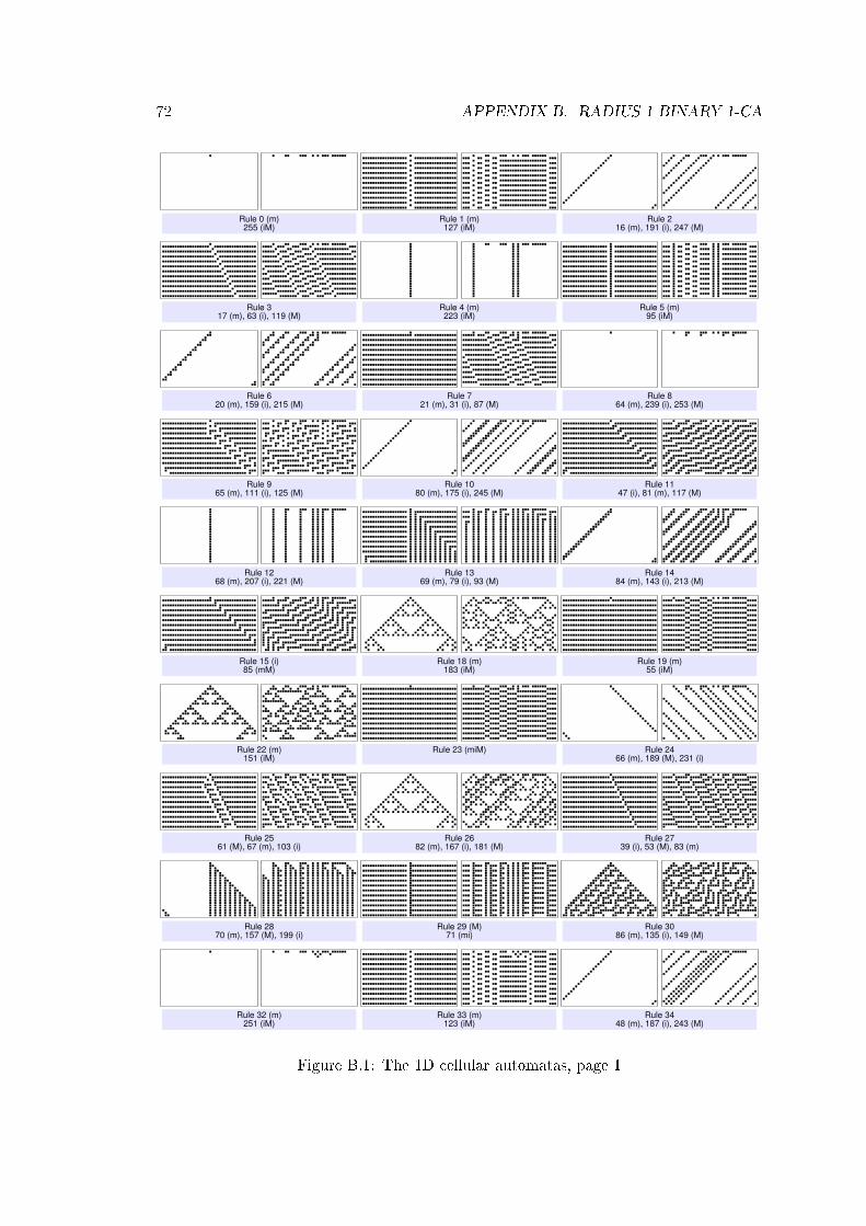
72 APPENDIX B. RADIUS 1 BINARY 1-CA
Rule 0 (m)255 (iM)
Rule 1 (m)127 (iM)
Rule 216 (m), 191 (i), 247 (M)
Rule 317 (m), 63 (i), 119 (M)
Rule 4 (m)223 (iM)
Rule 5 (m)95 (iM)
Rule 620 (m), 159 (i), 215 (M)
Rule 721 (m), 31 (i), 87 (M)
Rule 864 (m), 239 (i), 253 (M)
Rule 965 (m), 111 (i), 125 (M)
Rule 1080 (m), 175 (i), 245 (M)
Rule 1147 (i), 81 (m), 117 (M)
Rule 1268 (m), 207 (i), 221 (M)
Rule 1369 (m), 79 (i), 93 (M)
Rule 1484 (m), 143 (i), 213 (M)
Rule 15 (i)85 (mM)
Rule 18 (m)183 (iM)
Rule 19 (m)55 (iM)
Rule 22 (m)151 (iM)
Rule 23 (miM) Rule 2466 (m), 189 (M), 231 (i)
Rule 2561 (M), 67 (m), 103 (i)
Rule 2682 (m), 167 (i), 181 (M)
Rule 2739 (i), 53 (M), 83 (m)
Rule 2870 (m), 157 (M), 199 (i)
Rule 29 (M)71 (mi)
Rule 3086 (m), 135 (i), 149 (M)
Rule 32 (m)251 (iM)
Rule 33 (m)123 (iM)
Rule 3448 (m), 187 (i), 243 (M)
Figure B.1: The 1D cellular automatas, page 1

73
Rule 3549 (m), 59 (i), 115 (M)
Rule 36 (m)219 (iM)
Rule 37 (m)91 (iM)
Rule 3852 (m), 155 (i), 211 (M)
Rule 4096 (m), 235 (i), 249 (M)
Rule 4197 (m), 107 (i), 121 (M)
Rule 42112 (m), 171 (i), 241 (M)
Rule 43 (i)113 (mM)
Rule 44100 (m), 203 (i), 217 (M)
Rule 4575 (i), 89 (M), 101 (m)
Rule 46116 (m), 139 (i), 209 (M)
Rule 50 (m)179 (iM)
Rule 51 (miM) Rule 54 (m)147 (iM)
Rule 5698 (m), 185 (M), 227 (i)
Rule 57 (M)99 (mi)
Rule 58114 (m), 163 (i), 177 (M)
Rule 60102 (m), 153 (M), 195 (i)
Rule 62118 (m), 131 (i), 145 (M)
Rule 72 (m)237 (iM)
Rule 73 (m)109 (iM)
Rule 7488 (m), 173 (i), 229 (M)
Rule 76 (m)205 (iM)
Rule 77 (miM)
Rule 7892 (m), 141 (i), 197 (M)
Rule 90 (m)165 (iM)
Rule 94 (m)133 (iM)
Rule 104 (m)233 (iM)
Rule 105 (miM) Rule 106120 (m), 169 (i), 225 (M)
Figure B.2: The 1D cellular automatas, page 2

74 APPENDIX B. RADIUS 1 BINARY 1-CA
Rule 108 (m)201 (iM)
Rule 110124 (m), 137 (i), 193 (M)
Rule 122 (m)161 (iM)
Rule 126 (m)129 (iM)
Rule 128 (m)254 (iM)
Rule 130144 (m), 190 (i), 246 (M)
Rule 132 (m)222 (iM)
Rule 134148 (m), 158 (i), 214 (M)
Rule 136192 (m), 238 (i), 252 (M)
Rule 138174 (i), 208 (m), 244 (M)
Rule 140196 (m), 206 (i), 220 (M)
Rule 142 (i)212 (mM)
Rule 146 (m)182 (iM)
Rule 150 (miM) Rule 152188 (M), 194 (m), 230 (i)
Rule 154166 (i), 180 (M), 210 (m)
Rule 156 (M)198 (mi)
Rule 160 (m)250 (iM)
Rule 162176 (m), 186 (i), 242 (M)
Rule 164 (m)218 (iM)
Rule 168224 (m), 234 (i), 248 (M)
Rule 170 (i)240 (mM)
Rule 172202 (i), 216 (M), 228 (m)
Rule 178 (miM)
Rule 184 (M)226 (mi)
Rule 200 (m)236 (iM)
Rule 204 (miM)
Rule 232 (miM)
Figure B.3: The 1D cellular automatas, page 3

Index
2-cells, 452-neighbourhood, 442-rule, 442-transition map, 45
A, 12at, 12A New Kind of Science, 11abbreviations, 1action, 13ai vs. ai, 13alphabet, 7, 12atto-fox problem, 37
Baas, Nils A., 43behaviour, 13Belousov-Zhabotinsky, 33blinker, 31Buckingham, David J., 31Burks, Arthur Walter, 10
C, 13CA, 1, 10canonical lookup table, 15canonicalizing, 48caterpillar, 31cell, 8, 12
alive, 30dead, 30healthy, 33ill, 33infected, 33
cellular automata, 510, 121-dimensional, 183-state, 16chaotic, 20
class I, 19class II, 19class III, 20class IV, 21classication system, 19drawing by hand, 6famous, 30injective, 13isomorphic, 18labeling, 14numbering, 14outer totalistic, 17programming, 11recreational, 11repeating, 19reversible, 13surjective, 13survey of, 11totalistic, 17
cellular automaton, 1higher order, 1
Codd, Edgar Frank, 10code, 17codes
code 1599, 25computer algorithm, 12conguration, 8, 13
nite, 13initial, 10random, 34
Conway, John, 10Cook, Matthew, 21cyclic space, 9
d-CA, 12d1, 14
75

76 INDEX
Dewdney, Alexander Keewatin, 37dierential equations, 37d∞, 14
evolution, 13
f , 12sh, 37follows, 13forest re, 9formula, 12function, 8
G, 13g, 17Game of Life, 9, 10, 30Garden-of-Eden congurations, 13Gardner, Martin, 10Gerhardt, Martin, 33glider, 30, 31global function, 13
bijective, 13global state, 8, 13, 19
homogenous, 19initial, 13
gnuplot, 68Gosper, William, 48
h, 17hashing, 48Helvik, Torbjørn, 43higher order cellular automaton, 1HOCA, 1hodgepodge machine, 9
IBM, 37inhibitor, 27instructions, 6
Kusch, Ingo, 27
L, 12lattice, 7, 12
nite, 19innite, 19
Life, see Game of Lifelimit set, 17local transition function, see LTFLotka-Volterra, 37, 60LTF, 12
canonical lookup table, 15explicit form, 15, 19
manhattan norm, 1, 14map, 1Markus, Mario, 27Mathematica, 11maximum norm, 1, 14memoization, 48Moore neighbourhood, 16Moore, Edward F., 13morphological level, 44Myhill, John, 13
N , 12NM , 14Nr, 14NvN , 14neighbourhood, 8, 12, 14
conguration, 8rst neighbours neighbourhood, 14Moore neighbourhood, 14radius > 1, 23radius neighbourhood, 8, 14state, 8, 15, 16sum of states in, 17von Neumann neighbourhood, 14
neighbourhood conguration, 44neighbourhood state, 8notation, 1
organs, 45oscillators, 31
P, 1Palladium Oxidation, 33patterns
stationary, 21predator, 37prey, 37
INDEX 77
quadtree, 48quiescent state, 13quiescent states, 12
rule, 8rules
inverted, 18mirror, 18mirror-inverse, 18rule 28, 49rule 0, 19rule 110, 21rule 12, 20rule 135, 18rule 149, 18rule 150, 20rule 160, 19rule 24, 20rule 255, 49rule 30, 6, 18, 20rule 32, 19rule 4, 20rule 40, 19rule 8, 19rule 86, 18rule 90, 20symmetric, 18total number of, 16
S, 12Schuster, Heike, 33Scientic American, 10, 37seashell patterns, 27second level alphabet, 45self-replicating automatic factories, 10set, 1
of all integers, 1of non-negative numbers, 1
sets of sets, 1sharks, 37simple programs, 11spaceship, 30, 31speed of light, 31state, 8, 10, 12
statesmore than 2, 23
still life, 31support, 13
trac CA, 9
Ulam, Stanisªaw, 10universal computation, 21
vector, 1von Neumann, John, 10
Wolfram|Alpha, 11Wolfram, Stephen, 11, 15, 17, 19
bxe, 1bxc, 1
Z, 1~z, 1zi, 1Zn, 1Z+, 1