A stochastic programming approach to cashmanagement in banking

Jordi CastroDept. of Statistics and Operations Research

Universitat Politecnica de CatalunyaPau Gargallo 5, 08028 Barcelona (Catalonia, Spain)

jordi.castro@upc.edu

Research Report DR 2004-14December 2004

Revised August 2005, June 2007, October 2007

Report available from http://www-eio.upc.es/~jcastro

A stochastic programming approach to cash

management in banking

Jordi Castro

Dept. of Statistics and Operations Research

Universitat Politecnica de Catalunya

Jordi Girona 1–3

08034 Barcelona, Catalonia, Spain

jordi.castro@upc.edu

http://www-eio.upc.es/~jcastro

Abstract

The treasurer of a bank is responsible for the cash management ofseveral banking activities. In this work we focus on two of them: cashmanagement in automatic teller machines (ATMs), and in the compensa-tion of credit card transactions. In both cases a decision must be takenaccording to a future customers demand, which is uncertain. From histor-ical data we can obtain a discrete probability distribution of this demand,which allows the application of stochastic programming techniques. Wepresent stochastic programming models for each problem. Two short-termand one mid-term models are presented for ATMs. The short-term modelwith fixed costs results in an integer problem which is solved by a fast(i.e. linear running time) algorithm. The short-term model with fixedand staircase costs is solved through its MILP equivalent deterministicformulation. The mid-term model with fixed and staircase costs givesrise to a multistage stochastic problem, which is also solved by its MILPdeterministic equivalent. The model for compensation of credit card trans-actions results in a closed form solution. The optimal solutions of thosemodels are the best decisions to be taken by the bank, and provide thebasis for a decision support system.

Keywords: stochastic programming, OR in banking, integer stochastic pro-gramming

1 Introduction

Cash—or liquidity—management is one of the main concerns of a bank. Thisclass of problems appears in several of the usual banking activities. In this workwe focus on two relevant ones: cash management in automatic teller machines

1

(ATMs)—which is similar to cash management in branches—, and in the com-pensation of credit card transactions. In both cases the bank must advance someamount of money. This amount must be determined according to a future un-known probabilistic demand. If the demand is higher or lower than the amount,the bank incurs some problem specific penalty costs. These decision problemsresult in nontrivial extensions of the classical newsvendor problem, which areaddressed in this work through stochastic programming techniques. Good in-troductions to stochastic programming are Birge and Louveaux [1], Kall andWallace [8]. Briefly, stochastic programming problems are optimization prob-lems (either linear, integer or nonlinear) with one or several stochastic modelparameters. Stochastic programming has previously been used for decision mak-ing under uncertainty, both for generic decision support methodologies [11], andin particular decision support systems for other liquidity management activitiesin banking [4].

Cash management in ATMs (and similarly in branches) is a well-known prob-lem faced by any bank. The purpose is to decide the optimum amount of moneythat will be placed in the ATM to satisfy an uncertain demand. If the demandexceeds the amount in the ATM, the bank incurs in costs due to refilling tasks.It is worth to note that refilling is performed by external companies. There-fore, from the bank point of view, location of warehouses, costs associated totransportation, etc., are irrelevant. In practice, money transportation compa-nies offer two policies. In the first one, the bank pays a significant fixed fee (e.g,50e) for the refilling, independently of the amount, plus a small extra cost foreach fraction of a certain amount of money transported (e.g., 0.59e for eachfraction of 10000e); in this option we basically deal with fixed costs. In the sec-ond one, the fixed fee is small (e.g., 20e) while the staircase costs are significant(e.g., 30e for each fraction of 6000e). The above figures are close to the realones used by some Spanish money transportation companies. It is thus possibleto consider both models, one with only fixed cost—which is solved in linear timeby a specialized algorithm introduced in this paper—, the other with both fixedand staircase costs. In addition, the paper analyzes two different situations: theshort-term problem, with one single refilling; and the mid-term problem, whitmore than one refilling, which forces a multistage stochastic problem. All theabove considerations make this problem significantly different from the classicalnewsvendor problem. Several integrated decision support systems in the market[12, 13] implement optimization/simulation procedures for cash management inATMs, but no details are given about the particular techniques used.

The Spanish credit card system is based on a daily compensation mechanismbetween banks and a central agent that collects all credit card transactions.Each bank daily maintains an account, where the central agent charges all thetransactions from credit cards owned by this bank. The crucial decision for thebank is what amount to daily maintain in that account, given the uncertainoverall sum to be charged. We will see that particular instances of this problemcan be solved through inventory techniques with stochastic demands [14, Ch.17]. For a general model, we must rely on other more versatile procedures, asstochastic programming.

2

As far as we know, stochastic programming has not previously been usedfor the two problems of this work, although it was in many other financialapplications (few of them are described, for instance, in Dantzig and Infanger[2], Golub et al. [5], Gondzio and Kouwenberg [6], Kallberg et al. [7], and manymore can be found in the books Ziemba and Mulvey [17], Zenios and Ziemba[16], and the surveys Kouwenberg and Zenios [9], Yu et al. [15] and the morethan 150 references therein). The stochastic programming approach used inthis work is clear, easy to implement, very efficient, and provides the optimalsolution according to the future possible set of scenarios. The application of thisprocedure may improve current techniques used by banks, which are based onsimulation, experience and trial and error. Even with the current low interestrates, which anyway have been successively increasing in the last months in theEuropean Union, a better solution to the problem is relevant. For instance, thefinancial group ”La Caixa” (one of the biggest of Spain, located in Barcelona)owns near 7000 ATM’s and 5000 branches. Assuming that an average dailyamount of l e is currently disposed at each ATM, and interest rates of r%, asolution that reduces the daily amount per ATM in just a p% would result inan overall benefit of 0.7 · r · l · p e per year. Using realistic values l = 100000,r = 3, an improvement of p = 5 results in 1.05 million e per year.

The paper is structured as follows. Section 2 outlines the general formulationof the stochastic optimization problems used in this work. Section 3 describesand solves the stochastic models for the cash management problem in ATMs.Section 4 presents and solves the stochastic formulation of the cash managementproblem in the compensation of credit card transactions.

2 The stochastic programming problem

In the two-stage stochastic programming problem a set of first-stage decisionsx ∈ R

n1 must be taken before the values of some stochastic parameters, de-pendent of random variable ξ, are known. The cost of first-stage decisions isrepresented by c(x). Once ξ is known, we must adjust another set of second-stage variables y ∈ R

n2 to minimize the costs we incurred by our choice of x andthe particular value of ξ; the function of second-stage costs is Q(x, ξ). We lookfor the decisions x that, in average, according to the distribution of ξ, providethe minimum costs. The general model (with fixed recourse) is

minx

c(x) + Q(x)

subject to x ∈ X ⊂ Rn1 ,

(1)

where

Q(x) = Eξ[Q(x, ξ)] and

Q(x, ξ) = miny

q(y; ξ)

subject to Wy = h(ξ) − T (ξ)xy ∈ Y ⊂ R

n2 .

(2)

c(x) and x ∈ X in (1) are usually a linear function cx and a convex polyhedrondefined by X = {x : Ax = b, x ≥ 0}, respectively. Integrality constraints x ∈ Z,

3

either for a subset or for all the first-stage variables, may also appear in (1).Q(x), known as the recourse function, is the future average cost of our first-stage decisions x, for all scenario (i.e., for all realization of ξ). q(y; ξ) and y ∈ Y

in (2) are usually a linear function q(ξ)y and nonnegativity constraints y ≥ 0,respectively. Integrality constraints y ∈ Z can also appear in y ∈ Y , either fora subset or for all the second-stage variables; indeed we will need them in thecash management problem for ATMs. The stochastic parameters of this generalformulation are q(ξ), h(ξ) and T (ξ). In the models of next sections only h(ξ) isstochastic, and is defined as h(ξ) = ξ, ξ being the customers demand of money,either from the ATM or through the credit card.

For some particular problems we can obtain a closed form solution forQ(x, ξ) = q(y∗; ξ), y∗ being the optimum second-stage decisions. In these caseswe may be able to “compute” Q(x) = Eξ[Q(x, ξ)], either evaluating the expec-tation (e.g., for discrete distributions or some low dimensional random variable)or approximating it (e.g., for multidimensional continuous variables) (see [1,Ch.9] for details). This allows the solution of (1) only in terms of the first-stage decisions. We will apply this strategy in the models of Subsection 3.1 andSection 4.

In general, however, no closed form exists for Q(x, ξ) and we are forced tosolve the extensive form or deterministic equivalent of the stochastic problem.For this purpose we consider ξ is a discrete random variable of s values ξ1, . . . , ξs

with probabilities p1, . . . , ps . Each particular value ξi, i = 1, . . . , s is usuallyknown as a scenario. Replicating for each scenario the second-stage variables(i.e, yi, i = 1, . . . , s) and constraints, and combining problems (1) and (2), weobtain the following (probably large) problem:

minx,yi

c(x) +

s∑

i=1

piq(yi; ξi)

subject to x ∈ X

Wyi = h(ξi) − T (ξi)xyi ∈ Y

}

i = 1, . . . , s.

(3)

Problem (3) can be solved with standard linear, integer or nonlinear program-ming algorithms if it is of moderate size; otherwise we need to apply specializedprocedures that exploit the particular problem structure [10, 1, Ch. 5–8]. Themodel of Subsection 3.2 will be solved by a state-of-the-art MILP package.

Multistage stochastic problems generalize the above two-stage framework,involving a sequence of observation-decision events. For k stages, they can beformulated as

minxi

c1(x1) + Eξ2

[

min c2(x2(ξ2); ξ2) + · · · + Eξk

[

min ck(xk(ξk); ξk)]

· · ·]

subject to W1x1 = h1

W2x2(ξ2) + T1(ξ

2)x1 = h2(ξ2)

Wixi(ξi) + Ti−1(ξ

i)xi−1(ξi−1) = hi(ξ

i) i = 3, . . . , k

x1 ≥ 0, xi(ξi) ≥ 0 i = 2, . . . , k,

(4)

4

where Wi, i = 1, . . . , k are known mi×ni matrices, h1 is a known vector in Rm1 ,

hi, i = 2, . . . , mi are random vectors in Rmi , Ti, i = 1, . . . , k−1 are mi× (ni−1)

random matrices, xi ∈ Rni , i = 1, . . . , k is the vector of decisions at stage i

(such that xi, i > 1, depends of previous random events), and ξi means thehistory of random events up to stage i. In that formulation we have implicitlyrestricted our decisions to depend on past data, and they must be the same atstage i for scenarios with a common history up to stage i−1. In a deterministicequivalent formulation we must include explicit nonanticipativity constraints tomodel such behaviour (see [1] for details). The model of Subsection 3.3 will besolved by a three-stage stochastic model.

3 Cash management in ATMs (and branches)

The objective is to find the amount of cash to be disposed in an ATM for a cer-tain period of time (e.g., one week-end, one week) using a stochastic program-ming approach. The same model can basically be also used for cash managementin branches. We need the following information:

• Historical data m1, m2, . . . , mt of the overall amount of money due totransactions in the ATM or branch, during last t periods (e.g., days). mi

can be either positive (i.e., money injected into the ATM or branch) ornegative (i.e., money extracted from the ATM or branch). In practicewe should differentiate depending on the type of period, e.g., workable,weekend, holidays, etc. We assume our data corresponds to the same typeof periods. Banks record all the transactions performed in an ATM (andbranch), and thus the historical data mi is exhaustive. It is known thatthe empirical cumulative distribution function (cdf) is the maximum like-lihood estimate of the real cdf [3, p. 310]. Because of the efficiency ofthe procedure described below, we will consider the empirical probabilitydistribution ξ of values ξi and probabilities pi, i = 1, . . . , s,

∑s

i=1 pi = 1,population data. That means that for all i ∈ {1, . . . , t} we guarantee thatsome scenario j ∈ {1, . . . , s} satisfies ξj = mi. Usual techniques in stochas-tic programming for estimating sampling distributions, as bootstrapping,can thus be avoided.

• l ≥ 0, u > 0 (l < u): minimum and maximum allowed amount of moneyin the ATM or branch. For an ATM u is its technical capacity. l can bea reserve fixed by law, mainly for branches. Values 0 and ∞ can be usedif these bounds are not applicable.

• c ≥ 0: Cost per e in the ATM or bank branch for the time horizonconsidered in the problem. This cost is associated with interest rates, andit may also include insurance costs for the money disposed in the ATM.

• k ≥ 0: Fixed cost for the refilling or extraction of money if the ATM orbranch gets out the allowed bounds l and u. This cost is independent of

5

the amount of money refilled. It is used in the models of Subsections 3.1,3.2 and 3.3.

• kv ≥ 0, v ≥ 0: cost for each fraction of ve disposed in the ATM or branch.This cost defines the staircase costs of models of Subsections 3.2 and 3.3,and it is used in conjuction with the fixed cost defined by k above.

We analyze three realistic situations. The first two correspond to a short-term period of few days, e.g., one week-end, or some short period of holidays.In that case, at most one single refilling may be necessary. Depending of thepolicy considered by the money transportation company, we have two differentmodels: the first one only considers fixed costs k associated to refilling, whereasthe second also uses the staircase costs associated to kv. An O(s) algorithm ispresented for the fixed cost problem, whereas the other is solved formulatingthe deterministic equivalent. The third model applies to a mid-term period,e.g., one week. Current practice in banking is to refill twice per week, since onesingle refill is not enough for the existing demand. This results in a multistageoptimization problem, which is again solved by its deterministic equivalent.

3.1 The short-term problem with fixed costs

We define x ∈ R as the amount of money to be placed in the ATM or branch.Indeed we should impose x ∈ Z, but as shown below we will always obtain aninteger solution. This is the first-stage decision to be optimized in our two-stagestochastic program. For the second-stage we define a binary variable z ∈ {0, 1};z is 1 if the ATM has to be refilled, otherwise is 0. We also need auxiliarysecond-stage variables y+ ∈ R and y− ∈ R. The final formulation is

minx

cx + Eξ[Q(x, ξ)]

subject to l ≤ x ≤ u(5)

whereQ(x, ξ) = min

z,y+,y−kz

subject to x + ξ + y+ ≥ l

x + ξ − y− ≤ u

y+ ≤ Mz

y− ≤ Mz

z ∈ {0, 1}, y+ ≥ 0, y− ≥ 0,

(6)

M being a large enough value (e.g., M = maxi{|ξi|, i = 1, . . . , s}). Constraintsof (6) force that the amount placed in the ATM plus the future demand isbetween bounds (l ≤ x + ξ ≤ u). If this can not be satisfied then we needa positive value for the auxiliary variables y+ or y−, and thus z must be 1,inducing refilling costs.

The deterministic equivalent of the above stochastic formulation is obtainedby replicating the second-stage variables for each scenario (i.e, zi, y+

i , y−i , i =

6

1, . . . , s), and the constraints where they intervene. It gives rise to the followingMILP problem.

minx,zi,y

+i

,y−i

cx + k

s∑

i=1

pizi

subject to l ≤ x ≤ u

x + ξi + y+i ≥ l

x + ξi − y−i ≤ u

y+i ≤ Mzi

y−i ≤ Mzi

zi ∈ {0, 1}, y+i ≥ 0, y−

i ≥ 0

i = 1, . . . , s.

(7)

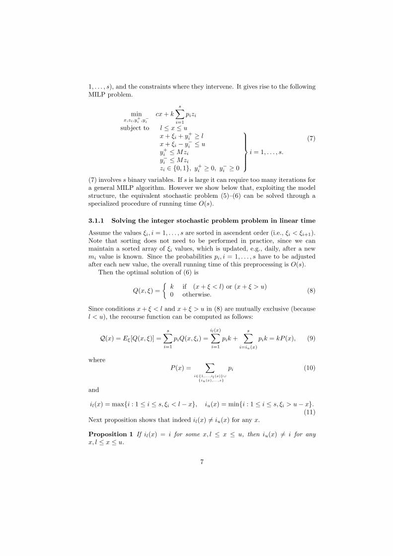
(7) involves s binary variables. If s is large it can require too many iterations fora general MILP algorithm. However we show below that, exploiting the modelstructure, the equivalent stochastic problem (5)–(6) can be solved through aspecialized procedure of running time O(s).

3.1.1 Solving the integer stochastic problem problem in linear time

Assume the values ξi, i = 1, . . . , s are sorted in ascendent order (i.e., ξi < ξi+1).Note that sorting does not need to be performed in practice, since we canmaintain a sorted array of ξi values, which is updated, e.g., daily, after a newmi value is known. Since the probabilities pi, i = 1, . . . , s have to be adjustedafter each new value, the overall running time of this preprocessing is O(s).

Then the optimal solution of (6) is

Q(x, ξ) =

{

k if (x + ξ < l) or (x + ξ > u)0 otherwise.

(8)

Since conditions x + ξ < l and x + ξ > u in (8) are mutually exclusive (becausel < u), the recourse function can be computed as follows:

Q(x) = Eξ[Q(x, ξ)] =

s∑

i=1

piQ(x, ξi) =

il(x)∑

i=1

pik +

s∑

i=iu(x)

pik = kP (x), (9)

whereP (x) =

∑

i∈{1,...,il(x)}∪

{iu(x),...,s}

pi (10)

and

il(x) = max{i : 1 ≤ i ≤ s, ξi < l − x}, iu(x) = min{i : 1 ≤ i ≤ s, ξi > u − x}.(11)

Next proposition shows that indeed il(x) 6= iu(x) for any x.

Proposition 1 If il(x) = i for some x, l ≤ x ≤ u, then iu(x) 6= i for anyx, l ≤ x ≤ u.

7

Proof. From (11), il(x) = i means that x < l − ξi; since l ≤ x, then ξi < 0.Let’s suppose that for some x, iu(x) = i. From (11) and u ≥ x, we haveu ≥ x > u − ξi, and then ξi > 0, which is a contradiction.�

The deterministic equivalent problem to be solved is

minl≤x≤u

cx + kP (x). (12)

To compute cx + kP (x) we must know the il(x) and iu(x) indexes for eachinterval of x values. From the definition (11), considering that l ≤ x ≤ u, andusing an artificial value ξs+1 = ∞, we have that

il(x) = i, 1 ≤ i ≤ s, if x ∈ [max{l− ξi+1, l}, min{l− ξi, u})] = [ai, bi)]. (13)

Abusing of notation, “)]” means that the right endpoint is either or not includedin the interval: if u < l − ξi, then the interval is [ai, bi], otherwise it is [ai, bi).An interval such that bi < ai means that il(x) is never i, for any value x; thoseintervals are removed from consideration. Note that the intervals [ai, bi)] arecontiguous, i.e., bi = ai+1. From (11), indices iu(x) are defined similarly, usingan artificial value ξ0 = −∞,:

iu(x) = i, 1 ≤ i ≤ s, if x ∈ [(max{u−ξi, l}, min{u−ξi−1, u}] = [(ci, di]. (14)

As before, “[(” means that the left endpoint is either included or not; it is ifl > u − ξi, otherwise it is not. As for il(x), an interval with ci < di meansthat iu(x) is never i, for any value x, and it is discarded. The intervals [(ci, di]are contiguous too. From the above intervals [ai, bi)], [(ci, di), P (x) can becomputed as

P (x) =

il∑

i=1

pi +s∑

i=iu

pi, where

il =

{

i if ∃i : x ∈ [ai, bi)]0 otherwise

, iu =

{

i if ∃i : x ∈ [(ci, di]s + 1 otherwise

.

(15)Consider for instance a small example for a short period of three days, with

s = 4, ξ = (−130,−80,−50, 50) with probabilities p = (0.2, 0.3, 0.4, 0.1), l = 20,u = 140, c = 0.00025 (which corresponds approximately to an annual interestrate of 3%) and k = 0.05. ξ, l, u, k and x are expressed in 1000’s e. Values k,l, u, and c are real ones, whereas ξ has been chosen for illustrative purposes (ina real situation, s ≫ 4). The first three values of ξ represent an extraction ofmoney from the ATM; the last scenario ξ4 represents an injection. Using (13)and (14) we obtain the following [ai, bi)] and [(ci, di] intervals:

il(x) =

1 if x ∈ [100, 140]2 if x ∈ [70, 100)3 if x ∈ [20, 70)4 if x ∈ [20,−30) not possible

8

Figure 1: a) cx and kP (x) for the example. b) cx + kP (x) for the example

x

0.0

0.03

40

0.02

80 120

0.05

0.04

0.01

0

kP(x)

cx

0.06

x

80

0.07

0.05

0.03

0.0

0.01

120

0.04

40

0.02

0

cx+kP(x)

a) b)

and

iu(x) =

1 if x ∈ (270, 140] not possible2 if x ∈ (220, 140] not possible3 if x ∈ (190, 140] not possible4 if x ∈ (90, 140]

The resulting cx, kP (x) and cx + kP (x) functions of the example are shownin Figure 1. Note that the interval (90, 140] for iu(x) = 4 overlaps intervals[70, 100) and [100, 140] for il(x) = 2 and il(x) = 1, respectively, giving rise tothe new ones [70, 90], (90, 100) and [100, 140]. As shown by next propositionthe number of final intervals in P (x) is at most 2s. Abusing of notation and tosimplify the cases in the proof, we will assume intervals for il(x), iu(x) and thosedue to overlapping are of the form [(ai, bi)], [(ci, di)] and [(ej , fj)] (as before,“[(”, “)]” means that the endpoint is either included or not).

Proposition 2 Let [(ai, bi)], i = 1, . . . , sl ≤ s be the intervals for il(x) and[(ci, di)], i = 1, . . . , su ≤ s those for iu(x). The number of new intervals [(ej , fj)]due to overlapping is, at most, 2s.

Proof. We assume the intervals are ordered, i.e., ai+1 = bi, ci+1 = di. This as-sumption is guaranteed if intervals are computed by (13) and (14). The interval[(ci, di)] may overlap some [(aj , bj)] intervals, resulting in new ones. There arefour cases, listed below. The first two are the nontrivial ones, while the last tworeduce to one of the first two cases.

a) The endpoints of [(ci, di)] belong to the same interval [(aj , bj)], i.e., aj ≤ci ≤ di ≤ bj . Figure 2.a) illustrates this situation. The resulting threeintervals are [(aj , ci)], [(ci, di)], and [(di, bj)], increasing by one the numberof original two overlapping intervals.

9

Figure 2: Two nontrivial cases for overlapping intervals. a) Interval [(ci, di)]is contained in interval [(aj , bj)]; b) Interval [(ci, di)] starts and ends in twodifferent intervals [(aj , bj)] and [(aj+l, bj+l)].

New intervalsNew intervals

Interval

ilInterval

iuInterval

ilIntervals

ui

a) b)

b) The endpoints of [(ci, di)] belong to different intervals [(aj , bj)] and [(aj+l, bj+l)],l ≥ 1, i.e, aj ≤ ci ≤ bj ≤ aj+l ≤ di ≤ bj+l, as shown in Figure2.b). The resulting l + 3 intervals are [(aj , ci)], [(ci, bj)], [(aj+1, bj+1)],[(aj+2, bj+2)],. . . , [(aj+l, di)], [(di, bj+l)], increasing by one the number oforiginal l + 2 overlapping intervals.

c) The left endpoint of [(ci, di)] is less than a1, the leftmost point of all[(ai, bi)] intervals, i.e., ci < a1 ≤ di. We then create one new interval[(ci, a1)], an apply to the remaining portion of [(ci, di)], namely [(a1, di)],one of cases a), b) or d).

d) The right endpoint of [(ci, di)] is greater than bsl, the rightmost point of

all [(ai, bi)] intervals, i.e., ci < bsl≤ di. We then create one new interval

[(bsl, di)], and apply to the remaining portion of [(ci, di)], namely [(ci, bsl

)],one of cases a), b) or c).

Therefore, for any interval [(ci, di)] that overlaps with intervals [(ai, bi)] one newone is created at most. Since, from Proposition 1 sl+su, the number of intervals[(ai, bi)] and [(ci, di)], is at most s, the number of new intervals created is atmost 2s. �

Since cx has always a positive slope, the minimum of cx+P (x) is on the leftpoint of one of the intervals due to overlapping. It is thus sufficient to evaluatecx + P (x) in at most 2s points to obtain the optimal solution. It is worth tonote that if ξi, i = 1, . . . , s, l and u are integer values, then the left points ofall the intervals will also be integer and the procedure will report an integersolution. Algorithm of Figure 3 shows the main steps of the procedure, whichis a constructive proof of the following result:

Proposition 3 The integer stochastic programming problem (5)–(6) for cashmanagement in ATMs can be solved in polynomial time using algorithm of Figure3. Moreover, the running time is O(s), s being the number of scenarios.

10

Proof. It is immediate from the discussion of previous paragraph that algorithmof Figure 3 solves (5)–(6). Moreover, the running time of steps 1–4 of algorithmof Figure 3 is O(s), and then the overall procedure is O(s). �

Figure 3: Procedure for the solution of problem (12)

Algorithm Cash Management ATM :1 Compute intervals of x [ai, bi)] i = 1, . . . s using (13)2 Compute intervals of x [(ci, di] i = 1, . . . s using (14)3 Obtain new intervals of x [(ei, fi)] i = 1, . . . l ≤ 2s due to overlapping4 i∗ = arg min{cei + kP (ei), i = 1, . . . , l}5 Return: x = ei∗

End algorithm

Looking at Figure 1, the final number of intervals is four, and the optimalsolution is x = 100 (100,000e to be put in the ATM for the time period consid-ered) —the left point of interval [100, 140]— with an expected cost of 0.04 (40efor the period). Solving (7) for this example through a MILP solver the samesolution is obtained.

3.2 The short-term problem with fixed and staircase costs

Extending formulation (5) we obtain the following model for this second situa-tion:

minx

cx + Eξ[Q(x, ξ)]

subject to l ≤ x ≤ u(16)

where

Q(x, ξ) = minz,y+,y−,nv

kz + kvnv

subject to x + ξ + y+ ≥ l

x + ξ − y− ≤ u

y+ ≤ Mz

y− ≤ Mz

y+ ≤ nvv

y− ≤ nvv

z ∈ {0, 1}, nv ∈ N, y+ ≥ 0, y− ≥ 0,

(17)

nv being the number of fractions of ve disposed to or removed from the ATM.

11

Although the solution of (17) is given by

Q(x, ξ) =

k + kv

⌈

l − (x + ξ)

v

⌉

if x + ξ < l

k + kv

⌈

(x + ξ) − u

v

⌉

if x + ξ > u

0 otherwise,

(18)

the expression of Q(x) can not be easily computed, unlike in (9). We then haveto resort to the following deterministic equivalent formulation

minx,zi,y

+i

,y−i

,nvi

cx + k

s∑

i=1

pi(zi + kvnvi)

subject to l ≤ x ≤ u

x + ξi + y+i ≥ l

x + ξi − y−i ≤ u

y+i ≤ Mzi

y−i ≤ Mzi

y+i ≤ nvi

v

y−i ≤ nvi

v

zi ∈ {0, 1}, nvi∈ N, y+

i ≥ 0, y−i ≥ 0

i = 1, . . . , s.

(19)

Although (19) has s binary variables and s integer ones, in practice, it can beefficiently solved by state-of-the-art MILP solvers. Table 1 shows the computa-tional results for some instances generated from the example used in Subsection3.1. The realistic values considered, expressed in 1000’s e, are l = 20, u = 140,c = 0.00025 (which corresponds approximately to an annual interest rate of3%), k = 0.02, kv = 0.03 and v = 6. First instance of 4 scenarios of demandof money corresponds to the example of Subsection 3.1. The scenarios for theother instances were randomly generated from the same theoretical distribution,a normal of µ = −65 and σ = 20, which explains the same optimal value in allcases. We used a theoretical distribution for the demand because we have noaccess to such a confidential information. The runs were performed on a PCwith one AMD Athlon 4400+ 64 bits dual core processor, using the AMPL mod-elling language and the solver CPLEX 9.1. For each intance, Table 1 shows thenumber of scenarios (column s), optimal first stage decision in 1000’s e (x∗),number of overall simplex iterations (MIP iter.), the number of branch-and-bound nodes explored (B&B nodes) and the overall CPU time (CPU). Clearly,it is shown that, unlike the specialized algorithm of Subsection 3.1, the CPUtimes do not linearly increase. However, an optimal solution is provided in fewseconds.

3.3 The multistage mid-term problem

For a mid-term planning (e.g. one week), models of Subsections 3.1 and 3.2are not applicable, since they only consider a single refilling. Current technical

12

Table 1: Solution of (19) for pseudo-randomly generated instancess x∗ MIP iter. B&B nodes CPU4 138 8 0 0.016

100 114 243 6 0.0641000 114 7352 434 4.275000 114 35567 837 35.33

capacities of ATM’s and customers demand of money force two or more refilloperations, depending of the time horizon. In theory we can consider any num-ber h of refill operations, giving raise to a (h+1)-stages stochastic problem. Asfor the model of Subsection 3.2, we will consider fixed and staircase costs forthe refill operations. The general (h + 1)-stages model can be formulated as anextension of (16)–(17):

minx

cx1 + Eξ2,...,ξh+1

[

h∑

t=2

cxt +

h+1∑

t=2

(

kzt + kv(n+v,t + n−

v,t))

]

subject tol ≤ xt−1 ≤ u

bt = bt−1 + xt−1 + ξt + y+t − y−

t

l ≤ bt ≤ u

y+t ≤ Mzt

y−t ≤ Mzt

y+t ≤ n+

v,tv

y−t ≤ n−

v,tv

zt ∈ {0, 1}, y+t ≥ 0, y−

t ≥ 0n+

v,t ∈ N, n−v,t ∈ N

t = 2, . . . , h + 1

b1 = 0.

(20)

ξt, t = 2, . . . , h + 1 are the demands for the t-th stage. bt, t = 1, . . . , h is theamount of money in the ATM at stage t prior to decision xt (initially b1 = 0,though any other value could be used). Unlike previous models, the amountof money refilled or extracted, y+

t and y−t , is bounded by different n+

v,t, n−v,t

variables. This allows the inclusion of both variables y+t and y−

t in the moneybalance equations. If necessary, dependency of random variables between stagescould be added to (20), i.e. ξt+1|(t,t−1,...,1).

The above problem can not be solved through a special algorithm, as we didin Subsection 3.1, and we are forced to use the deterministic equivalent formu-lation. Although in theory any number h of refill operations can be considered,we will restrict to a three-stage situation, i.e., h = 2. This is the current practicein Spain for weekly periods, where refill operations are scheduled by some banksfor Tuesday and Friday. The deterministic equivalent of this three-stage modelis given by

13

Table 2: Solution of (21) for pseudo-randomly generated instancess2 s3 s x∗ MIP iter. B&B nodes CPU50 20 1000 133 1219 0 0.1450 50 2500 133 2161 367 10.8775 50 3750 121 18431 12638 316.99

100 50 5000 124 11426 6631 602.3†

† stopped by CPU time limit, with a relative optimality gap of 0.006

minx

s∑

i=1

pi

(

3∑

t=2

(

cxt−1i+ kzti

+ kv(n+v,ti

+ n−v,ti

))

)

subject tol ≤ xt−1i

≤ u

bti= bt−1i

+ xt−1i+ ξti

+ y+ti− y−

ti

l ≤ bti≤ u

y+ti≤ Mzti

y−ti≤ Mzti

y+ti≤ n+

v,tiv

y−ti≤ n−

v,tiv

zti∈ {0, 1}, y+

ti≥ 0, y−

ti≥ 0

n+v,ti

∈ N, n−v,ti

∈ N

t = 2, 3i = 1, . . . , s

b1i= 0 i = 1, . . . , s

additional nonanticipativity constraints.

(21)

As usual, nonanticipativity constraints force same decisions at stage t for scenar-ios with a common history up to stage t−1 (e.g., for x1 they could be x11 = x1j

for all s ≥ j > 1). Problem (21) has 2s binary, 4s integer and 8s continuousvariables, such that s =

∑s2

i=1 s3i, s2 and s3i

being the different values of ξ2 andξ3|2i

.Table 2 shows the computational results for some instances. As for Table 1,

we used the realistic values (expressed in 1000’s e) l = 20, u = 140, c = 0.00025(related to an annual interest rate of 3%), k = 0.02, kv = 0.03 and v = 6.The different values for ξ2 and ξ3 were randomly generated from the same twotheoretical distributions, a normal of µ = −65 and σ = 20 for ξ2, and µ = −80and σ = 15 for ξ3, since we have no access to real-world —thus confidential—values. The runs were performed on a PC with one AMD Athlon 4400+ 64bits dual core processor, using the AMPL modelling language and the solverCPLEX 9.1. For each instance, Table 2 shows the number of values for ξ2

(column s2, which corresponds to the number of nodes of the second stage inthe scenario tree), number of values for ξ3 (column s3), number of scenarios(s = s2 · s3 in these runs), optimal first stage decision in 1000’s e (x∗), numberof overall simplex iterations (MIP iter.), the number of branch-and-bound nodesexplored (B&B nodes) and the overall CPU time (CPU). Compared to those of

14

previous sections, this model is computationally more expensive. However it isstill possible to obtain optimal or near-optimal solutions to small and mid-sizeproblems in seconds or minutes of CPU.

4 Cash management in the compensation of creditcard transactions

In the Spanish system there is a central agent that daily records all the bankscredit card transactions and performs the payments from some accounts ownedby these banks. Banks must guarantee a certain amount for such paymentsin their particular account. If the account becomes empty the central agentperforms the remaining payments, lending money to the bank at a high inter-est. Otherwise, if the bank decides to maintain a large amount of money in theaccount, it causes an excess of overstock costs associated with interest rates.That problem can be seen as an inventory problem with stochastic demands, inparticular as a newsvendor problem. However, we will consider a stochastic pro-gramming formulation, which is more general and can be easily accommodatedto extra constraints and nonlinear cost functions. The information required forthe model is:

• Historical data m1, m2, . . . , mt of the daily credit card payments madeby the bank customers during last t days. As in Section 3, from thisdata we generate the empirical probability distribution ξ of values ξi andprobabilities pi, i = 1, . . . , s, which is the maximum likelihood estimate ofthe real cdf. We will also differentiate depending on the type of day.

• l ≥ 0, u > 0 (l < u): minimum and maximum capacity of money in theaccount (set 0 and ∞ if not applicable).

• c1 ≥ 0: Cost per e in the account, due to interest rates.

• c2 > 0: Cost per e lent by the central agent (c2 > c1).

Let x be the amount of money in the account, and let y+ be the moneylent by the central agent and y− the residual money in the account after thepayments. These are respectively the first and second-stage decisions. Theformulation is

minx

c1x + Eξ[Q(x, ξ)]

subject to l ≤ x ≤ u(22)

whereQ(x, ξ) = min

y+,y−c2y

+

subject to x + y+ − y− = ξ

y+ ≥ 0, y− ≥ 0.

(23)

15

This is a two-stage stochastic problem with simple recourse. The solution of (23)is y+∗

= max{ξ − x, 0}, y−∗= max{x − ξ, 0}. The recourse function can thus

be easily computed as Q(x) = Eξ[c2y+∗

]. Alternatively, we can use a generalexpression of Q(x) for simple recourse problems where the only stochastic termis the right-hand side of the second-stage problem [1, p. 93]. Applying thisexpression of Q(x) in (22) we obtain

minx

g(x) = c1x + c2

(

ξ − x + F (x)x −∫

ξ≤xξf(ξ)dξ

)

subject to l ≤ x ≤ u,(24)

f(ξ) and ξ being respectively the density function and the expected value of thedaily payments. (24) is an optimization problem of one variable with simplebounds. If ξ is continuous, g(x) is a convex continuous function of derivative

g′(x) = c1 + c2(F (x) − 1). (25)

If bounds are inactive, the optimal solution satisfies g′(x∗) = 0. If ξ is dis-crete then F (ξ) has discontinuities at points ξi, i = 1, . . . , s, and g(x) is convexpiecewise linear and its subdifferential is

∂g(x) ={

π|c1 + c2(F (x) − 1) ≤ π ≤ c1 + c2(F+(x) − 1)

}

, (26)

where F+(x) = limξ↓x F (ξ). If bounds are inactive, a point x∗ such that 0 ∈∂f(x∗) is optimum. Therefore, either for a continuous or discrete distribution,the solution is:

x∗ =

l if F (l) > 1 − c1

c2≥ 0

u if F (u) < 1 − c1

c2≤ 1

F−1(1 − c1

c2) otherwise.

(27)

For a discrete distribution given by the sample m1, m2, . . . , mt, which is theusual case in practice, the quantile F−1(1 − c1

c2) is computed by first sorting in

ascendent order the above data, obtaining m(1), m(2), . . . , m(t), and then finding

the position i =⌈

t(1 − c1

c2) − 1

⌉

. The solution is

x∗ = m(i+1). (28)

If we allow interpolation then we can alternatively use

x∗ = m(i) + (t(1 −c1

c2) − i)(m(i+1) − m(i)). (29)

In some numerical tests performed, the extensive form of (22–23) solved with alinear programming code provided the first solution (28). Note that, if bounds l

and u are not active, the solution F−1(1− c1

c2) is equivalent to F−1( cu

co+cu), which

we would have obtained by considering an inventory problem with stochastic de-mands, and understock and overstock costs cu = c2−c1 and co = c1, respectively[14, Ch. 17]. However, the stochastic programming approach is more versatile,

16

allowing lower and upper bounds l and u, and even the solution of generaliza-tions of the problem. A realistic one would be to consider a convex or piecewiselinear objective function in (23), i.e., the larger the value of y+—money lentby the central agent—, the larger the interest rates or penalization applied. Inthis case we can solve the deterministic equivalent of the new stochastic model,which is a linear programming problem.

5 Conclusions

Several banking activities currently performed in some institutions simply bysimulation, experience or trial and error, can effectively be optimized by stochas-tic programming techniques. In this work we focused on models for two partic-ular activities: cash management in ATMs and in the compensation of creditcard transactions. For basic models of both problems we provided very efficientprocedures for computing the best decision ahead of an uncertain money de-mand. For extensions of the ATM model (i.e., short and mid-term problemswith fixed and staircase costs) the MILP deterministic equivalent formulationswere solved.

The models for cash management in ATMs and compensation of credit cardtransactions considered can be extended in several ways to fit the particularbank reality. For instance, the cash management models for ATMs could dealwith situations where only some type of bills (e.g., 20e) are exhausted. In thiscase there is likely no need to refill the ATM, but the bank incurs costs due todissatisfaction of customers, who are forced to get multiples of, e.g., 50e. Bothproblems can also be extended with nonlinear or piecewise linear cost objectivefunctions in the second stage. For some of these extensions it can even bepossible to obtain a specialized solution procedure, as those presented in thiswork. Otherwise, we must solve the extensive form of the problem, as we didfor the two-stage and multistage cash management models with staircase costs.This could mean a larger, but hopefully yet reasonable, solution time. However,this is not a main drawback, since decisions in this context are not taken inreal-time, but periodically.

6 Acknowledgments

The author is indebted to the staff of the Spanish division of a worldwide bank,who suggested and detailed the problems dealt with in this work. We have beenasked to maintain confidential both the names of the persons and the bank. Theauthor also thanks two anonymous referees whose suggestions clearly improvedthe presentation of the work. This work has been partially supported by theSpanish MEC grant MTM2006-05550.

17

References

[1] J.R. Birge, F. Louveaux. 1997. Introduction to Stochastic Programming,Springer, New York.

[2] G.B. Dantzig, G. Infanger. 1993. Multi-stage stochastic linear programs forportfolio optimization, Annals of Operations Research 45 59-76.

[3] B. Efron, R.J. Tibshirani. 1993. An Introductoin to the Bootstrap, Chap-man & Hall, London.

[4] F. Gardin, R. Power, E. Martinelli. 1995. Liquidity management with fuzzyqualitative constraints, Decision Support Systems 15(2) 147–156.

[5] B. Golub, M. Holmer, R. McKendall, L. Pohlman, S.A. Zenios. 1995.Stochastic programming models for money management, European Journalof Operations Research, 85(2) 282–296.

[6] J. Gondzio, R. Kouwenberg. 2001. High performance computing for assetliability management, Operations Research 49(6) 879–891.

[7] J.G. Kallberg, R.W. White, W.T. Ziemba. 1982. Short term financial plan-ning under uncertainty, Management Science, 28 670–682.

[8] P. Kall, S.W. Wallace. 1994. Stochastic Programming, Wiley, Chich-ester. Available electronically from http://www.unizh.ch/ior/Pages/-

Deutsch/Mitglieder/Kall/bib/ka-wal-94.pdf.

[9] R. Kouwenberg, S.A. Zenios. 2006. Stochastic programming models for as-set liability management, in: Stavros Zenios and Bill Ziemba (eds.), Hand-book of Asset and Liability Management, series Handbooks in Finance,Elsevier, 253–303.

[10] W.K. Klein Haneveld, M.H. van der Vlerk. 1999. Stochastic integer pro-gramming: General models and algorithms, Annals of Operations Research85 39–57.

[11] D.C. Novak, C.T. Ragsdale. 2003. A decision support methodology forstochastic multi-criteria linear programming using spreadsheets, DecisionSupport Systems 36(1) 99–116.

[12] Transoft Inc. 2004. OptiCa$h. http://www.transoftinc.com/opticash.htm.

[13] Wincor/Nixdorf. 2004. ProCash Analyzer. http://www.-

wincor-nixdorf.com/internet/us/Products/Software/Banking/-

CashAnalyzer/index.html.

[14] W.L. Winston. 1994. Operations Research. Applications and Algorithms,3rd ed., Duxbury Press, Belmont.

18

[15] L.-Y. Yu, X.-D. Ji, S.Y. Wang. 2003. Stochastic programming models infinancial optimization: A survey, Advanced Modeling and Optimization5(1) 1–26.

[16] S. A. Zenios, W.T. Ziemba. 2006, 2007. Handbook of Asset and LiabilityManagement, Vols. 1 and 2, series Handbooks in Finance, Elsevier.

[17] W.T. Ziemba, J.M. Mulvey. 1998. Worlwide asset and Liability Modelling,Cambridge University Press.

19