A Statistical Approach to Quantum Mechanics*courses.physics.ucsd.edu/2017/Spring/physics142/Labs/FinalProject/... · STATISTICAL APPROACH TO QUANTUM MECHANICS 429 X FIG. I ... where

ANNALS OF PHYSICS 132, 427-462 (1981)

A Statistical Approach to Quantum Mechanics*

M. CREUTZ AND B. FREEDMAN

Physics Department, Brookhacen National Laboratory, Upton, New York I1973

Received November 13, 1980

A Monte Carlo method is used to evaluate the Euclidean version of Feynman’s sum over particle histories. Following Feynman’s treatment, individual paths are defined on a discrete (imaginary) time lattice with periodic boundary conditions. On each lattice site, a continuous position variable xi specifies the spatial location of the particle. Using a modified Metropolis algorithm, the low-lying energy eigenvalues, / &,(x)jZ, the propagator, and the effective potential for the anharmonic oscillator are computed, in good agreement with theory. For a deep double-well potential, instantons were found in our computer simulations appearing as multi-kink configurations on the lattice.

I. INTRODUCTION

Feynman’s path integral formulation of quantum mechanics reveals a deep connection between classical statistical mechanics and quantum theory. Indeed, in an imaginary time formalism the Feynman integral is mathematically equivalent to a partition function. Using this analogy, particle physicists have recently employed a well-known technique of statistical mechanics in using Monte Carlo simulation to study gauge field theories [ 1, 21. The simulations are a means of numerical evaluation of the path integrals. This has yielded new non-perturbative insight into the behavior of quantized Yang-Mills fields.

A gauge system is a rather complicated quantum theory with many degrees of freedom. This masks the connection between a Euclidean Monte Carlo treatment and a more traditional Hilbert space formulation of quantum mechanics. In this paper we search for such connections by studying a considerably simpler model, a one- degree-of-freedom SchrGdinger system. We will see how Monte Carlo methods can provide information on the ground and first excited states of this problem. We do not advocate these methods for accuracy, rather we hope they may lead to better understanding of the workings of the Monte Carlo method. Furthermore, these methods are rather easily generalizable to systems with many degrees of freedom.

This paper is organized as follows. In Section II we review the Feynman formalism and present the formulas we will use in our numerical studies. Section III presents and

* This paper was authored under Contract DE-A02-76CHOO016 with the U.S. Department of Energy. Accordingly, the U.S. Government’s right to retain a nonexclusive, royalty-free license in and to the copyright covering this paper, for governmental purposes, is acknowledged.

427 0003-4916/81,!040427-36$05.00~0

Copyright 0 1981 by Academic Press, Inc. All rights of reproduction in any form reserved.

428 CREUTZ AND FREEDMAN

justifies the Monte Carlo method for evaluation of these path integrals. Section IV contains some numerical results obtained from the simple harmonic and anharmonic oscillators. Section V is a brief conclusion and in the Appendixes we treat more carefully some technical details.

II. THE PATH INTEGRAL

In this section we will study the similarities between quantum theory and statistical mechanics. Our fundamental tool will be the Euclidean (imaginary time) version of Feynman’s sum over histories [3]:

0.1)

Both representations of Z require explanation: The vectors / xi) and 1 xr) in Eq. (2.1) are position eigenstates, If is the Hamiltonian

operator for a spinless particle of mass m, moving in a potential, where

H(P, Q) = P2/mo + W?), (2.2)

and T is a positive number. Equation (2.1) is of interest because, if we expand in a complete set of energy eigenstates,

then

ff I n> = En I n) (2.3)

zri = 2 e-EnT’“(xf / n)(n 1 xi). n

(2.4)

Thus, at large T the leading term in this expression gives us the energy and wavefunction of the lowest-lying energy eigenstate.

The second form for Z must also be explained. The Euclidean action is given by

s = JOT dr [+m, [$I’ + v(x)],

where 7 = it (t is real time), and s [dx] denotes integration over all functions X(T) obeying the boundary conditions

x(0) = xi ) (2.6a)

and

x(T) = Xf . (2.6b)

STATISTICAL APPROACH TO QUANTUM MECHANICS 429

X

FIG. I. Making time discrete to label paths.

The original version of Feynman’s Path Integral is of the form

2(x, , xi) = C exp &/I?, paths

(2.7)

where the sum is over all world lines that connect the initial and final points, and S,, is the Minkowski space action for a particular path. A precise definition of the “sum over all paths” must be provided before Eq. (2.7) becomes useful. One way to proceed is to introduce a time lattice, so that various paths can be labelled simply (Fig. 1). Making the time axis discrete, we adopt the following notation:

X(tj) = Xi (.i = 0, I,..., N), (28

where - co < xj < co for all sitesj, and

'j+1 - tj = E, (2.9)

where E is the spacing between adjacent time slices. Expression (2.7) is a sum of rapidly oscillating phases. By continuing to imaginary time each path will be weighed by an ordinary damped exponential factor, making it easier to distinguish important paths from unimportant paths. This is our Euclidean Path Integral given in Eq. (2.1). The integration measure is now well defined and is given by

z,i - 1-T ycl dxj exp (- f S[Xjl) (N- cQ>, (?.lOj


where T == Na. The action for a discrete time lattice is just

(2.11)

where a =~ ie. We use the boundary conditions x,, = xi and XN = xf . The continuum limit is recovered by letting N ----f co and a -+ 0, keeping T fixed. For later use we define the trace of ZYj

Equation (2.10) is identical to the partition function for a statistical mechanics problem. We have a one-dimensional lattice with sites labeled by index j. On each site there is a variable xj , which takes on continuous values as given by (2.8). The action couples nearest-neighbor variables xj and xj+r , and the integral J” JJ,“=7’ dxj is really a sum over all possible lattice configurations. The Boltzmann factor is just

e-l /ri.qZl 3 (2.12)

where /I = temperature, and the Euclidean action, (2.11). is the classical Hamiltonian for a system with N degrees of freedom.

In statistical mechanics the temperature is a measure of the statistical fluctuations in a system, while in quantum mechanics ti is a measure of the quantum fluctuations (through the uncertainty principle). In quantum mechanics, the h + 0 limit picks out classical physics. In particular, as fi + 0 the classical trajectory for a particle moving in a potential V(x) becomes the only path that contributes to the transition amplitude Zfi , fluctuations are completely suppressed. As T approaches zero for a statistical system, fluctuations are frozen out. These points allow for a one-to-one correspondence between doing quantum mechanics in imaginary time and statistical mechanics on a real crystal lattice.

Since Z is a partition function we can also define a free energy for our lattice, namely

Z = e-fiF (F = free energy), (2.13a)

F = - 1 In Z, P

(2.13b)

where /I = l/r%. Because F is an extensive quantity, it is useful to define a free energy density f, where F = f. T, and T is the volume of our (time) crystal. Equation (2.13) now becomes

-1 f = mlnZ, (2.14)

STATISTICAL APPROACH TO QUANTUM MECHANlCS 431

which as T---f cc yields

,f’ = E, . (2. I 5)

As in statistical mechanics, it is useful to measure correlation functions, which are given formally by

r(n) = Tr ,-HT,ily _ (71) x(72) *a. x(7,)/2, (2.16a)

where

In quantum theory the P) are called n-point propagator functions. We can write Eq. (2.16) in a compact form by defining

Z(J) = Tr e ~T,fi[H+~;J,zil 9 (2.17)

where Ji is an external c-number current (SJJSJ, = &). Then we have

From the logarithm of Z we obtain the connected n-point functions

p = s. I: SJ, ... & In zfJ) I/=,, . (2.18)

For example,

p := ~!X(T1) .Y(T2)1 - (S(T1)\‘./X(T*)“,

where we have adopted the notation

(2.19)

(d) = Tr(e-HT/“A)/Tr(e-~T/~) (2.20)

for any operator d. In terms of the functional (path) integral, (2.20) is equivalent to the expression:

(2.21)

where now A(.\- r ,..., x,) is just a normal function of the x’s. The propagators Pn) for a spin-system in statistical mechanics are the correlation functions

rg = /s,s, ... s,;,, (2.22)

where the Si are spin variables at sites {ij in the crystal.


In the limit T--f co, we recover the expectation values of our operators in the quantum theory:

= (0 1 d/O), as T--t 00. (2.23)

In this case, the two-point fuuction rr’ becomes

kz p = <o 1 x(0) X(T) / 0) - (0 I x I O?a

(2.24)

We can find the energy gap between E1 and E,, by taking the large t limit in Eq. (2.24). Choosing 7’ > T + m, we see that

___ = e-(E1-EO) k-7) /s l-p’(Y) y’(T)

or

A (El - E,) = Fi (2 ln[ri2)(7 + Ll,)jP”‘(,)l). (2.25b)

To determine the lowest energy eigenvalue, E,, is in principle easy, since we know that

E0 = (0 / H 1 0) = Qrnm [Tr(e-HTlnH)/Tr e-HTIK]

Using the path integral representation for 2, Eq. (2.26a) becomes

(2.26a)

(2.26b)

Unfortunately, the expectation value of the action, (S), diverges like l/a for small lattice spacing. For any potential I’(x), the velocity-dependent part of (S) behaves in the following way:

(2.27)

Although a mean velocity can be defined, no mean-square velocity exists at any point. In other words, the important paths for a quantum-mechanical particle are non-


differentiable! Although these paths are very irregular, one possible remedy is to define the expectation of v2 following Feynman and Hibbs [3]

The expectation value in Eq. (2.28) is perfectly well behaved when a ---f 0. Eq. (2.28) is a split-point definition for vi2 and allows us to calculate E, for our system. Operators local in time, in contrast, have a nice continuum limit as a+ 0; no redefinition is necessary. An alternative procedure is to use the virial theorem to calculate the kinetic energy

&Mo(vi2;) = 3(x . V’(X)>, (2.29)

The ground-state energy is thus given by the formula:

E. = g++ (j [dx] ,-l'hs["][~xV'(x) + t'(x)]jj [dx] e-lins[zl). (2.30)

The ultimate goal is to evaluate the integrals in the partition function. For most potentials, however, analytic solutions simply do not exist. Furthermore, we must do N integrations, where N becomes infinite as a + 0. In the next section, we describe a numerical method for calculating the expectation values of operators [as in (2.21)] motivated, in part, by statistical physics.

III. EVALUATING PATH INTEGRALS

In this section we describe a technique for performing the sum “over paths” of the Feynman integral [4]. This approach is based on the Monte Carlo method of Metro- polis et al. [5].

Let us begin by defining the expectation value of any operator d for a finite time interval T as

(cd. = x A(x,) exp[-S(x,J]/C exp[-Wx,.)]. (3.1) I, 1.

where X~ denotes a configuration (or path) of the system. Each configuration depends on N dynamical variables {xi} which give the position of the particle at each timeslice {to. The action for a configuration xy = (xi’), xi” ... x$‘) is given by

S(x,) == F aLi?( x2,,, i=, (3.2)

where the Lagrangian couples nearest-neighbor variables and T = Na. In statistical mechanics, Eq. (3.1) corresponds to the canonical ensemble average of an operator A


for a system of N classical particles described by a Hamiltonian, HN t--f S. Noting that xi takes on one value from a continuous set of points

-cc < xi < co, (3.3)

we can write Eq. (3.1) more explicitly

(A> = J‘ BxA(x) exp[-S(x)]/J 9x exp[-S(x)]. (3.4)

The measure used in the functional integral is

The basic goal of the Monte Carlo method is to evaluate the “phase-space” sums or integrals in Eqs. (3.1), (3.4) numerically. We approximate an integral Jf(x) 9x by a sum with a finite number of terms xVf(x,) dx, . Note, however, that the integrand exp[-S(x,)] will vary over many orders of magnitude for moderately large time intervals T. Thus, a simple random sampling of points x, would be impractical for purposes of real computation. The Monte Carlo method introduced by Metropolis is based on the idea of “importance sampling.” Here the phase-space points x, in Eq. (3.4) are not selected completely at random, but are more densely distributed in that region of phase space giving the dominant contributions to the integrals. Motivated by statistical mechanics, we wish to choose states x, according to the Boltzman distribution

fyx,) 9x = exp[ --S(x,)] 9x J 23x exp[-S(x)] ’

(3.6)

Then the Monte Carlo estimate A for the quantity (A) simply reduces to an arith- metic average

A = $5 /4(x,), "=l

(3.7)

where M is the total number of states generated in the Monte Carlo sequence. The realization of “importance sampling” is possible using a Markov process to

generate the M configurations (x,> in Eq. (3.7) [6]. This process is constructed so that in the limit where A4 becomes infinite the probability of occurrence of configuration x, in the Markov chain is given by Eq. (3.6). It is useful to review the basic features of the Markov process since it figures so prominently in things to come.

A Markov chain is described by an N x N matrix W (N < co) with entries Wij >, 0 satisfying the condition

c wij = 1 (3.8)

STATISTICAL APPROACH TO QUANTUhZ MECHANICS 435

for all i. The idea is that W,j should represent the probability that a system, currently in state si makes a transition into a state sj in one Markov step. which we loosely refer to as one unit of time. Here the indices i and j label the possible configurations of the system. We can extend this definition to include continuous state spaces by defining a transition probability density, W(x, x’), for x ---f x’ satisfying

(3.9a)

and

J dx’ W(x, x’) := 1 (for all x). (3.9b)

In a two step process from .X to x’ (or si to Sj) the system must pass through some intermediate state x1 . The probability of a transition from x to X’ in two steps in a Markov chain is given by

W”‘(s, x’) = s

dx, W(x, x,) W(x, , x’). (3.10)

For a discrete system this would correspond to matrix multiplication. Similarly for an n-step process, we have

The long time behavior of the system can be approached by studying the limiting properties of lVn) as n ---f cc. Using properties (3.9) of the transition “matrix” it is possible to show that

!jm W’“)(x, 5’) = P*(x), (3.12)

for all x. In the large II limit, the transition probability function is independent of the initial configuration and is given by P*(X). For a discrete system, the lim,,,, Wij exists and is a matrix with identical rows. For the interested reader the proof of Eq. (3.12) can be found in Appendix B. In Eq. (3.1 l), taking n + IX shows that P*(x) is stationary in the sense that:

P*(d) = [ dYI,\-, P*(.x,) W(x, ) 2). (3.13)

fn other words, P* is a left eigenvector of M with an eigenvalue of unity. From Eq. (3.9), P*(x) also satisfies the condition of a probability distribution

P*(x) > 0 (for all x), (3.14a)


and

s dx’ P*(x’) = 1. (3.14b)

It is an easy matter to show P* is unique. Let P be another set of probabilities satisfying (3.13), and (3.14); then

P(x’) = j dxm P(xJ I+‘& , x’). (3.15)

Iterating Eq. (3.15) n times,

P(x’) = j- dx% P(x,) W’“‘(x, , x’). (3.16)

Allowing n + co in Eq. (3.16), we find

P(x’) = !ii J dx, P(xJ wyx, ) x’)

= dx, P(x,) P*(Y) s

= p*w, for all x’. (3.17)

Therefore, P* is the unique fixed point of the Markov process in the limit the chain becomes infinite.

To sumarize, we wish to construct W(x, x’) to satisfy

W(x, x’) > 0 (if P(x) > 0 and P(x? > o>, (3.18a)

I dx’ W(x, s’) = I, (3.18b)

P”q(x’) = f- dx Peq(x) W(x. x’), (3.18~)

where Peq is the same probability appearing in (3.6). Applying Win (3.18) n times to an initial ensemble Ei produces the following chain

Completely independent of our starting configuration Ei , we know that

lim E!“) = E*, Hi% 2 (3.20)

where E* is the equilibrium ensemble with probabilities given by (Pe”]. It is useful


to think of k!’ as an evolution operator in “ensemble space.” A point in this space is defined by the probabilities of our ensemble, that is

E = (PIE, PzE ,..., PjE ,... ). (3.21)

We can even go so far as to define a norm in this space

II E - E’I’ = t 1 pi - P; 1, i=l

(3.22a)

which in the continuum limit becomes

1~ E - E’;! = [ d.~ / P(x) - P’(x)[. (3.22b)

Figure 2 shows a Markov process for two different starting configurations E,., and EB . The time needed to reach E* will in general be different for these two cases. If our initial ensemble has a configuration close to E*, convergence will be rapid. it pays to make a good guess. There are ways of selecting a reasonable starting I$ which we shall describe later in this section.

We now turn to the task of explicitly constructing a transition probability W(x, x’) from the requirements of Eq. (3.18). Note that these requirements do not specify W

-x- _ 6 I J

i7 :8

I ,

t J

4\x I 09

5’x #ho ‘5&11

, /

E*

E*= (F’,*,P;)

, I I L __ _~_____-___~--._~ -~_.----.~.

0 PI I

FIG. 2. Approaching equilibrium from different directions.


uniquely. A simple choice by which Eq. (3.18) is fulfilled is provided by the detailed balance condition

wx, x’) ~~ P”q(x’) ____- Wx’, xl P”Q(x) .

(3.23)

Using (3.23) in Equation (3.18~) satisfies the requirement that Peq is an eigenvactor of f!P, since

Pyx’) = j dY Pqx) W(x, x’)

s P”qx’) = c/.x P”4(x) W(x’, x) peq(x)

= j dx W(x, x’) P”q(x’)

= P”‘I(x’). (3.24)

Equation (3.23) still does not specify W(x, x’) uniquely. Considerations of efficiency and computational feasibility eventually dictate its form. In our work we have followed the rather common procedure of probing the lattice variables one at a time, so that I+) and P+l) differ, at most, in the va x’)of a single variable Xj . Here we use the term “probing” to mean the effect of W(x --f x’) on the lattice at a certain time in the chain. For our procedure W is really a single step stransition probability ( IVS). The detailed balance condition for W, is extremely simple. Using Eq. (3.6) for Peq and keeping all but one variable, .Yj, fixed, we find

ws(x, x’) ,---S(Ji) ___-____ Wx’, x) e-s’“i’ ’ (3.25)

where S(Xj) is the action associated with Sj , and depends only on xj and its nearest neighbors. The Markov process is defined by probing successively all the statistical variables of the lattice many times. One complete sweep through the lattice is referred to as one Monte Carlo iteration. When all the spins have been analyzed, we proceed to a new iteration. The matrix defining the Markov process for a Monte Carlo iteration is given by

W’N’ = W,$(.& ) XN) w,s(x&-, ) XN-1) ... wdx; , x,) w&c; , Xl ). (3.26)

This still leaves open the detailed form of the transition probability W,(xf , .I-;). The most intuitive way to satisfy Eq. (3.25) is to pick

W,(Xj , Xi) - e 4x;) . (3.27)

Thus,the transition probability for a single step is proportional to the Boltzmann factor for X: . This method is referred to as the “Heat Bath” algorithm [I, 2, 71. ft has the feature that the variable being probed is always changed according to (3.27). Histori-


tally, the first method for solving (3.25) was introduced by Metropolis et al. [5], and is called the “Metropolis algorithm” (what else). It differs from the Heat Bath method in several important ways. The simplest form of W, in the Metropolis method is given

by

W,(.Uj , S:) --- + 11 . B[S(Xj) - S(Xj:)] + exp[-dS(xl , Xj)] B[S(-Y;) - S(X,)] 0

+ J” &‘[I - exp(--dS(x ; 7 .Kj)] d[S(X’) ~- S(.Uj)] 6(X: - Xj)\, (3.28)

where dS(.u’. .\-) = S(x’) ~ S(x), and Ai,, is the volume of the configuration manifold. Equation (3.28) looks incredibly complicated when compared with Heat Bath, however. it is by far the simpler of the two to implement in a real calculation.

To understand the simplicity of this algorithm, let us analyze (3.28) in some detail: The method of Metropolis begins by choosing randomly a new value X: with uniform probability. If the action is lowered by the replacement of Xj with xJ, the variable at sitej is set to this new value. If dS 2 0; then a random number r with uniform distribution between 0 and 1 is generated and “the variable is changed to .x: only if exp( -AS) ;:, r. Otherwise, the lattice variable retains its previous value, .yi . The next site is then probed in exactly the same way, and so on through the lattice. It is a simple exercise to check Eq. (3.28) satisfies (3.18a), (3.18b). To see that it also satisfies detailed balance let us choose x and x’ so that S(x’) <S(x). Then according to Eq. (3.28) W,(x. s’) m_ I and Ws(x’, x) = e-As(z,z’). C onversely, ifS(x’) > S(.u), then W,(x, x’) = L’~~~(,“‘..I’) and Ws(x’, x) = 1. The Metropolis algorithm reduces the distance of an ensemble from equilibrium by less per iteration than the heat bath: however, computational speed often more than compensates for this.

We have described only two methods for implementing detailed balance, there are certainly more. For example, it is often useful if the new state is rather close to the old one; in the Metropolis algorithm this is simply achieved by introducing a parameter d. Then xj 2 xi , where xj - d < xi < x, + d. This is extremely useful when the configuration space is large but the action highly peaked. The previous method would take a long time to change a configuration, since most of the new x’s would be rejected by the condition e-As > Y. Another modification can be made by increasing the number of Metropolis hits per site. This improves convergence to equilibrium, since a configuration change is more likely to take place:

x. A+ x!l) -!!i+ p + . . . -.+ x(‘i) W* 1 , I J 2 (3.29)

where X: is set equal to xjA) before proceeding to the next lattice site. Therefore, the algorithm we use is characterized by two additional parameters d and n, and satisfies, of course, Eqs. (3.18).

Finally, there is the matter of choosing an initial configuration close to E*. This clearly requires some prior knowledge of what the equilibrium ensemble looks like. In general this is known for only limiting cases of our system: at high temperatures (17 > 1) we expect the lattice to be random, while for low temperature (I? 4 0) classical


configurations of the action will dominate. Starting in either of these two configurations, we can then iterate systematically to tl = 1 (hopefully, both will agree!). For simple systems an educated guess will work almost as well, and saves a lot of computing time.

Usually we test for equilibrium by measuring some expectation value as a function of iteration time. We observe that average values of local operators settle down before we see the same numerical convergence in long range correlation functions. The notion of being in equilibrium is somewhat ill defined because the average value of one operator may “stabilize” before that of another. Our proof of a fixed point (E*) rested on taking n ---f co, making the Markov chain infinitely long. For finite n, deviations from E* will produce inaccuracies, the size of which can not be foretold. Different operators will be affected by this deviation from E* in different ways. In practice we always end- up working with finite chains, and so it is up to us to minimize the effects of j/ EC’“) - E* /I on the operator we are measuring by adjusting E, , A, and ii.

IV. NUMERICAL STUDIES

Our work has many features of an experiment. We work on a one-dimensional crystal, at a temperature equal to h, which comes into thermal equilibrium after a relaxation time. Once in equilibrium we measure the free energy, correlation functions, anything (in principle) we want. Our crystal has N degrees of freedom (xl , X, where each Xj is located at sitej on the lattice, and

XN),

(4.1)

(4.2)

The dynamics of our crystal is governed by the action

Here we consider the anharmonic oscillator potential

V(Xi) = $J.L2Xi2 + hXi4.

In our computer simulations, we worked on lattices with

N - lo2 to lo3 sites

(4.3)

(4.4)

(4.5)

Our choice for N, and a, was motivated by two considerations: (1) the lattice size, a, must be small enough to approximate the continuum limit; (2) Nu must be sufficiently


large to isolate the ground-state properties of our model. Defining TE = 27~h/E, we typically picked N and a so that

u/T~ - l/l0 to l/20,

NaiT, - 3 to 10.

(4.6a)

(4.6b)

Another problem is the size of statistical fluctuations in our crystal. For an operator f = CyZIJi , the relative fluctuation off about its average? is measured by

(4.7)

where Of = f’- f, and N is the number of lattice sites. To computef we average over NE “identical” crystals according to Eq. (3.7).

The time needed to reach equilibrium in units of Metropolis iterations was strongly dependent on lattice spacing but for moderately large a was typically found to be

Nt - 10 to 50 iterations (4.8)

depending on our choice for the initial lattice configuration. Using the Metropolis algorithm, we then generated NE lattice configurations. To keep members of our ensemble statistically independent of one another, 3-5 Monte Carlo iterations were made between lattice measurements. The Metropolis algorithm used in our computer simulations had

A -2 v’ii (4.9) and

fi-5to10. (4.10)

In most of our experiments NE - 10” gave reasonably small statistical fluctuations. Once in equilibrium, averages of moments and correlation functions

Xi’, Xi49 XiXi+nL y*.. (4.11)

were measured. But from Eq. (3.7), we also know that Eq. (4.11) is equivalent to

and

where r = ma.

(@> = XiP, (4.12a)

(W) a(T)> = XiXi+m 2 (4.12b)

Using Eqs. (4.11), (4.12), we were able to measure the low-lying states of the energy spectrum, E, and El _ These eigenvalues were computed from the following formulas:

E, = u”(x”) + 3h(x4) (virial theorem), (4.13)


T 1 - /

-LO -1 IO

0 I 2

x BIN NUMBER

FIG. 3. Binning the coordinates to study the ground-state wavefunction.

and

(4.14)

Likewise, we found the probability for finding a particle in the interval (x + dx, x - dx) from our data. Dividing the “x-axis” into bins of size Ax, we know that (see (A.26)):

j z,ho(x)~” = & Ny &Ax - I xi - x i,/ ;r I, (4.15) (21 z

where Ax is small. NToT = N ’ NE + GO, and the sum is over our Monte Carlo configurations. Equation (4.15) is pictured in Fig. 3, We chose Ax so a sufficient number of our events were recorded in each bin. Fluctuations in the jth bin behaved like --l/l/<, where aj was the number of times a trajectory passed through xi f Ax. N T O T was an extremely large number in our simulations -lo4 to 106.

A typical quantum trajectory from our Monte Carlo of the harmonic oscillator is shown in Fig. 4. The values of the potential parameters were m = 1.0, p2 = 1.0, h = 0. We worked on a 1000 site lattice with a = 0.1. Figure 5 shows the probability density for the ground state of the harmonic oscillator. Averaging over 300 Monte Carlo iterations, with N = 1000 and a = 1.0, we found the Monte Carlo points agreed with theory

1 z+Go(x)j2 = 0.59 exp -(l.l) x2 (4.16)

STATISTICAL APPROACH TO QUANTU’M MECHANICS 443

FIG. 4. A typical quantum trajectory for the harmonic oscillator.

r - - y - T -7 -_- - 7

HARMONIC OSCILLATOR ~

20

0 t -4.0

x

within statistical fluctuations -2 7:). Eq. (4.16) is the result one obtains for the discrete harmonic oscillator on a lattice this size and is derived in Appendix C. This is to be compared with the continuum answer (a --f 0)

(4.17)

In Fig. 5 we denote the points of our simulation by X’S, the lattice theory prediction by a dotted line, and the continuum result by a solid line. The potential V(X) and M, were the same as before.

A semi-log plot of the correlation function for the harmonic oscillator vs “time” separation t is shown in Fig. 6. The parameters used in this case were M,, = 0.5,

/Ii...---l-~...?-.- i -7--- I /

07 j

HARMONIC OSCILLATOR

FIG. 5. The ground-state probability density for the harmonic oscillator. The crosses are the Monte Carlo results, the dashed curve represents the discrete theory, and the solid curve gives the continuum theory.

595/132/2-I4

CREUTZ AND FREEDMAN

FIG. 6. The correlation between coordinates as a function of their time separation for the harmonic oscillator.

p2 = 2.0, h = 0, with N = 51 and a = 0.5. The x’s are our Monte Carlo points while the solid line is the theoretical prediction. The straight line in Fig. 6 indicates that only (0 1 2 II) is non-zero. This is correct for a harmonic oscillator since i - d - 8’. From Fig. 6 we find (x2> = 0.45, El - E,, = 1.98, and A, = 0.13 for NE = 100. These numbers should be compared to the theoretical values: (x2) = 0.447, I$ - E, = 1.975, A, = 0.11. Tn the limit a 4 0, (x2) = 0.5 and E, - E, = 2.0.

Figure 7 shows samples of quantum paths generated by Monte Carlo for the anharmonic oscillator. It is convenient to rewrite the potential (4.4) as

V(x) = h(x” - f2), (4.18)

where the zeros of the potential occur at the classical minima, x = &v’f2. This amounts to resealing S by an additive constant. For our computations we selected to keep X = 1, and vary f 2. Tn Figs. 7a-c we choose M,, = 0.5, a = 1.0, and N 7 50. We waited -40 iterations before recording the {x’s} in each case. The tunneling density was found to decrease rapidly as we varied f 2 from 0 to 2. Figure 7c shows a typical multi-kink configuration [8]. The dotted lines denote the positions of the classical minima of V(x) at x = @. Figure 8 is a graph of the ground-state probability 1 &,(x)j2 vs x for the value off 2 = 2.0. Using the parameters M, = 0.5, a = 0.25, N = 200, we averaged over 100 Monte Carlo iterations. The small number of tunnelings at large f 2 is reflected in the low probability around the origin in Fig. 8.

(b)

f*= I.0

STATISTICAL APPROACH TO QUANTUM MECHANICS

ANHARMONIC OSCILLATOR

445

(01

f’= 0.5

-X

ANHARMONIC OSCILLATOR ANHARMONIC OSCILLATOR

Cc)

f2=2 0

FIG. 7. Typical paths for the anharmonic oscillator for (a)f” = 0.5, (b)f2 ~7 1.0 and (c)f’ = 2.0.


2aNHARMONIC OSCILLATOQ 0 4+ l~~(J#

-2.0 -xc -1.0 0.0 1.0 xc 2.0

x

FIG. 8.; The ground-state probability distribution for an anharmonic oscillator.

Figure 9 is a semi-log plot of (x(0)x(~)) vs Q- for different choices of fi. Again Again f” 7: 2.0 was picked, with M,, = 0.5, a = 0.25, and N = 303. We performed an ensemble average consisting of 10 Monte Carlo iterations. Since we use periodic boundary conditions, we are actually averaging over 3,030 values of x(0)x(~) for each value of 7. We clearly must limit correlations of t/a < N/2. Increasing ii improved the Monte Carlo estimate of the correlation function with ?i N 15 giving the best results for this case. Choosing Ti too large will slow down the Monte Carlo simulation,

FIG. 9. Correlation versus time separation for the anharmonic oscillator.


FIG. 10. The first two energy levels of the anharmonic oscillator as functions of the parameterf2.

SO picking an optimal value for ii is necessary. Figure 10 is a plot of the low-lying energy levels vsf”. The solid lines are the known results from the continuum theory [9], the X’S are the Monte Carlo predictions. Unfortunately, the energy eigenvalues, {E,(J’“)j, are not available for comparison when N and a are finite, non-zero, numbers.

Coupling an external c-number source J to the site variables (xi) we studied the response of the crystal to an external current. The new action for the lattice is given by

S ---f S’ = S + J i xi, (4.19) i=l

where S is the old action. Since the new interaction breaks reflection symmetry, the expectation value (n), -~I xJ will not automatically vanish. Figure 11 shows sJ vs J for the harmonic oscillator. lt is straightforward to prove that when h = 0,

J = p2xJ (4.20)

for all a. In Fig. 11 we selected MO = 0.5, &I = 2.0, N = 51, and a = 0.1. The solid line is Eq. (4.20), the X’S are the results of our computer simulations. This experiment was repeated for the anharmonic oscillator, with A&,, = 0.5, f2 = 2.0, N = 303, and a = 0.25. The Monte Carlo curve is the dotted line in Fig. 12, the x’s are data points


J HARMONIC OSCILLATOR

--- -- <X)J

FIG. 11. The expectation x,, as a function of applied source J for the harmonic oscillator.

from our computer simulation. The solid line in Fig. 12 is a plot of the classical x, obtained by solving

J=-!p, (4.21)

and V(x) :z (x2 -f”)“. Using Figs. 11, 12 we can define a new function J(x,) for these two cases. Integrating

J(x,), we obtain a new function called the effective potential [IO]:

V,(XJ) = 1 dx’ J(x’). “3


FIG. 12. The expectation x,, as a function of J for the anharmonic oscillator.

(4.22)


HARMONIC OSCILLATOR

“R

0 XJ ANHARMONIC OSCILLATOR/ “R

/ K--c-.!: I:4:::4

-2 -I 0 I 2

0 XJ

FIG. 13. The effective potential for the harmonic oscillator. FIG. 14. The effective potential for the anharmonic oscillator.

Y&,) displays the true symmetries of the quantum theory-for this reason it can be thought of as the renormalized potential of the Hamiltonian. Figure 13 shows V,(x,) vs xJ for the harmonic oscillator. V,(x,) is identical to the classical potential V(x). Figure 14 shows the effective potential for the anharmonic oscillator. The effective potential in Fig. 14 has a single minimum at xJ = 0. This is not surprising since we know spontaneous symmetry breaking does not occur in quantum mechanics. Never- theless, it is amusing that we can compute V,(x,) using Monte Carlo techniques.

We can also isolate classical solutions [9] to the Euclidean equations of motion by sending fi -+ 0. For the anharmonic oscillator we can accomplish the same thing by making the barrier height larger (f” ---f co). We are specifically interested in finite action solutions which contribute to the transition probabilities

(x, I e-A’ / - x )

(-xc 1 e-AT ( xc;:

(4.23a)

(4.23b)

where x, = df>. These tunneling solutions will dominate over quantum fluctuations --O(A). To find a single kink we must impose antiperiodic boundary conditions

x(N + i) = -x(i), (4.24)

and f2 > 1. Figure 15 shows a single kink configuration for Mu = 0.5, fz = 2.0,


- 3.0 ANHARMONIC OSCILLATOR

f2=2 0

3.0 c

FIG. 15. A single kink configuration for the anharmonic oscillator with antiperiodic boundary conditions.

N = 200, and a = 0.25. The classical minima are denoted by *x, , and the classical turning points are at fx, and fx, . Figure 16 is a plot of x(t) vs t, where x(t) is a solution of mf = V’(x) satisfying

x(-T/2) = -xc ) (4.25a)

x(+772) = +x, , (4.25b)

where T is assumed to be large. These figures are in remarkable agreement.


f2: 2 0

FIG. 16. The classical tunnelling solution for imaginary time.



-30

FIG. 17. The annihilation of two kinks.

Figure 17 shows the Monte Carlo evolution of a kink pair under conditions where the equilibrium kink density is small. We worked on a 30 site lattice, a = 0.5, with symmetric boundary conditions. Our crystal was initialized with a two-kink configuration. After each pass through the lattice the new {xij’s were plotted, this was done 30 times. The potential was chosen to have

where x, = 2.0. With these parameters, the equilibrium density of kinks in our crystal satisfied

p;q . T< 1. (4.27)

Note how the two initial kinks attract and annihilate after roughly 18 iterations. It is well known that an n-kink state can decay into a smaller number of kinks, n + n’, so long as n + II’ = even. The simulation is consistent with this result. The amount of time for this to happen depended on the relative size of the quantum fluctuations to the kink-kink separation in our lattice.

V. CONCLUSION

In this paper we have shown how to apply Monte Carlo methods to the study of simple quantum systems. The method quite easily gives information about the ground state of a particle in arbitrary potential. The most serious shortcoming of the method


appears to lie in the study of levels beyond the first two. As the technique relies on an imaginary time formulation, the contribution of higher states are exponentially suppressed and therefore difficult to extract.

The main advantage of the method as applied to quantum mechanics is the almost trivial generalization to more degrees of freedom by adding more variables to the simulation. This has been dramatically illustrated by the successes of Monte Carlo studies of gauge theories. In going to a field theory, the time slicing used here generalizes to a space-time lattice. In addition to serving as a means of definition of the path integral, this lattice also provides an ultraviolet cutoff. This non-perturbative regulator gives control over the divergences which are rampant in quantum field theory.

The effective potential discussed in the last section will show its true value in higher dimensional field theories. Historically, it was introduced to study the spontaneous breaking of symmetries of the Hamiltonian. Tn addition, parameters characterizing the renormalized effective potential can be used in defining a renormalization scheme.

Finally we remark that Monte Carlo simulations in principle include all possible field configurations. If some particular type of excitations, i.e., topological, are physi- cally important, they should be seen upon careful examination of the simulated configurations. Thus we saw the “kink” configurations giving rise to tunneling phenomena in the anharmonic oscillator.

APPENDIX A: FUNDAMENTALS

Let us begin by considering a quantum mechanical system with one degree of freedom [12]. Let QH(t) be the position operator at time t in the Heisenberg picture:

where Q, = QH(0). The eigenstates of (L&(t) are defined by the condition

Q&> 14, t>~ = q 14, tjH 64.2)

or QSe-iHT / q, tjH = qeciHt I q, t)H , where q is the position coordinate at time t (it is just a c-number!). Now we define the states (I q)) as the eigenstates of QS with eigenvalue q:

Then we have

Qs I qj = q I s>. (A.3)

I 4, t>w = eiHt I 4). (A.4)

An especially interesting quantity in quantum theory is the transition matrix ,,(q’t’ 1 q, t)H which is the probability amplitude for the state prepared at t with the

STATISTICAL APPROACH TO QUANTUM MECHANLCS 453

coordinate ~7 to become the state of coordinate q’ at time t’. According to (A.4) this is given by

H(q’, t’ 1 q, tjH = (q’ 1 e-iH(t’~mt) / q). (A.9

We can imagine partitioning the time interval t’ - t into N segments, so that each segment goes to zero as N-t co. For simplicity, we shall divide the interval into N equal segments of duration d, such that

(t’ - t)/N = A. 64.6) Upon writing

e”H(t’-t) =e im--t, -l)eiH(t,-l-l,, z) . . _ eiH(t,--t) (A.7)

and inserting complete sets of eigenstates of Q, between the factors, we obtain

(q’ j e-iH(t’-t) 1 q) = J dq, **. J- dq&q’ I e-iffd 1 q&J

x (qnpl 1 euiHd 1 q,,-213 1.. c/q1 1 e-IHJ 1 4,;. (A.8)

We consider a Hamiltonian of the form H(P, Q), where

H(P, Q) = $P" f V(Q). G4.9)

Now for sufficiently small d we can factor (q’ / e-iHil / q) as follows:

(4’ I epiHd I q> = (4 I T I q> + CV),..., where

T = e-i/2V(Q)Ae-i/2P~Ae-i/2V(Q)A~ (A.lO)

This operator is called the transfer matrix [I I]. We can evaluate (A.10) by inserting a complete set of momentum eigenstates (1 p>} between the factors, where

BlP) -PIP,, (q I pj = @‘In.

(A.1 la)

(A.1 lb)

It is a straightforward calculation to show

(q’ I T j q) = 1 $ ei~.(rl’~~)e-iAH(/~.~.rl ), (A.12)

where H(p; q, q’) is an ordinary function Of the form

ff(p; q, 4’) = +JJz + f V(q) + 4 V(q’). (A.13)

When q’ ---f q, Eq. (A. 13) is just the classical expression for the Hamiltonian.

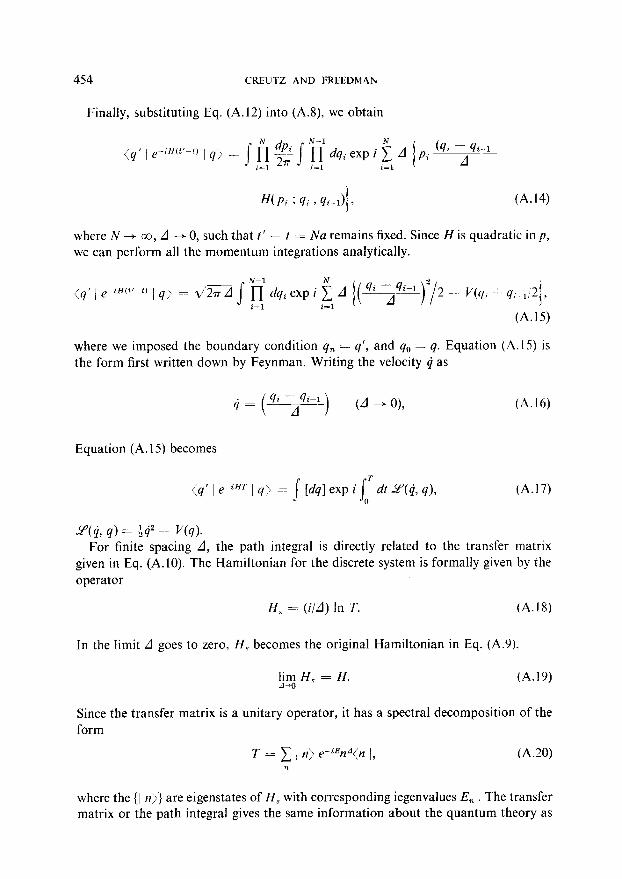
454

Finally, substituting

(4’ / e-iH(t’-f)

whereN+m,d+O, such that t’ - t = Na remains fixed. Since H is quadratic in p,

CREUTZ AND FREEDMAN

Eq. (A.12) into (A.8) we obtain

A p, (9i - 9i-1

I z A

(A.14)

we can perform all the momentum integrations analytically.

((/’ / e-iH(t’-t) 19.~ = 2//m j ‘z deli exp i i1 A I( 9i -A9i-1)2// - v((/~ -;- 4, ,;2/,

(A.15)

where we imposed the boundary condition qn = q’, and q, = q. Equation (A.15) is the form first written down by Feynman. Writing the velocity q as

4 = 9i - 9i-1

i A - 1 (A + 01, (4.16)

(9’ I epiHT I cl:> = j V91 exp i joT dt 2(4,9), (A.17)

w4, 9) = Q4” - U9).

Equation (A. 15) becomes

For finite spacing A, the path integral is directly related to the transfer matrix given in Eq. (A.10). The Hamiltonian for the discrete system is formally given by the operator

H,< = (i/A) In T. (A.18)

In the limit A goes to zero, H, becomes the original Hamiltonian in Eq. (A.Y),

$5 H, = H. (A.19)

Since the transfer matrix is a unitary operator, it has a spectral decomposition of the form

T = c 1 n) e-%zn”<n 1, (A.20) II

where the (I n>} are eigenstates of H, with corresponding iegenvalues En . The transfer matrix or the path integral gives the same information about the quantum theory as


solving Schrodinger’s equation, namely the spectrum of states, wavefunctions, and all the rest. In the continuum limit

T = exp - id[H + O(d)], (A.21)

which vve identify as the time-evolution operator for an infinitesimal step, d. The Schrbdinger picture is recovered by observing that the wavefunction is the

amplitude for finding a particle at x at time t regardless of how it got there. Therefore, the transition amplitude Z(s, t, x0 , to) is really a wavefunction. In fact, Z(x, t, x0, t,,) gives us more information than is required, since it also tells us that the particle started out at s,, at time t, . Using the rule for combining amplitudes, and identifying +(.I+, t) Z(s. t, 0, 0), we find that 4 must satisfy

+(i. f) = 1 d.y z(.u’, f, s, t) +(x, r). (A.22)

Choosing r’ ~ t = E to be infinitesimal, Eq. (A.22) becomes

$(x’, t’) = $(.I!, t) - icH$(x’, t),

where we used the fact

(A.23a)

Z(x’, t + E, x, t) -: lx’ 1 T 1 .Y/

: = ,(s’ ) I - icH 1 I‘,

=: 6(x’ - x) - ieH(.u)S(.u’ - s).

Equation (.4.23) is just the Schrodinger equation:

i$(x, t) = H(x) 4(x, t). (A.23b)

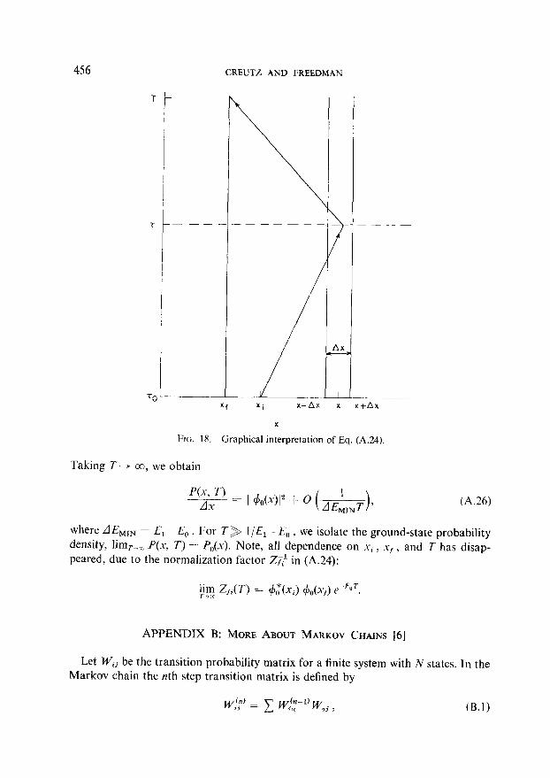
In Feynman’s version of quantum mechanics, the probability for finding a particle between .Y ~ AX and .Y i rls is just a time average over transition amplitudes (Fig. 18):

p(,; T) =: f j-r dt’ j’+“” dx’ Z(s, , T; I’, t’) Z(x’, t’, xi . 0)

Z(x, , T; 1-i , 0) ’ (A.24)

.x-JZ

Note, Eq. (A.24) keeps track of the number of times the particle passes through x with resolution AX during the time interval T. Let us assume dx is so small, that we can replace the integral over x’ by its value at X. Continuing (2.24) to imaginary time, and using Eq. (2.4) for Z,<, the time integration can be performed, yielding:


A---” *f Xi x-ox x x+Ax

x

FIG. 18. Graphical interpretation of Eq. (A.24).

Taking T+ co, we obtain

Pfx-, T) __- = Ax 1 +&>I” + ’ (A&), (A.26)

where AEMIN = El - E, . For T> l/E, - E,, , we isolate the ground-state probability density, lim,,, P(r, T) = P,,(x). Note, all dependence on xi, .xf, and T has disap- peared, due to the normalization factor 2%’ in (A.24):

APPENDIX B: MORE ABOUT MARKOV CHAINS [6]

Let Wii be the transition probability matrix for a finite system with N states. In the Markov chain the nth step transition matrix is defined by


where x.j Wij = 1, and W,, > 0 if PI and P, are greater then zero. Then the following is true:

exists, where 17 is a matrix with identical rows and satisfying the same properties as W. The proof that Wiy’ is independent of the initial state i is completely straightforward.

Assume first that n = 1, so that Wij > E > 0 for each i, ,j. Let 177~(?7) -= min, IQ;:’ denote the smallest element in thejth column of WC”), and similarly let Mj(n) be the largest element. Rewriting Eq. (B.l) as

then

W,‘;’ 3 C W~f,J?lj(lZ ~ 1) = 117,(17 - 1 ). (B.4)

Both (B.1) and (B.3) express W(“) as the matrix multiplication of W n-times. Since Eq. (B.4) holds for each i, it holds for the minimum, and so the column minima increase with 17,

fl?j(?7) ;I t?7j(r7 - I).

In just the same way we find the column maxima decrease with n. Therefore, both mj(n) and Mj(n) have limits as II + (;o. We must still show, however, that these two limits are the same.

To see this we estimate a little more carefully and we use (for the first time) the assumption that W<j 3 l . Suppose that the minimum mj(n) and the maximum Mj(n - 1) are attained when i = i, and i = i, , respectively. Then

z E I++-1’ + ( Wi,& - E) w/y $- c w; ,,,; w/f: l) 111 Kdi,

> l Mj(t7 - 1) + (1 - l ) lHj(t7 - I). (B.5)

In just the same way we find that

A4j(H) < Wj(17 - 1) + ( 1 - l ) Mj(H - I). (B.6)

Subtracting (5) from (6) yields

Mj(n) - T?Zj(n) 6 (1 - 2E)[Mj(t7 - 1) - tBj(fZ - I)], (B.7)


so that

M,(~I) - mj(n) < (I - 2~)” M [/V,(l) - 1)1j( I)]. (B.8)

From Eq. (B.8) we conclude that lim,.+,(Mj(n) - mj(n)) = 0. Suppose we choose m > 1, then we know in any case that

lim W(n’nl) = fl 9 (B.9) n-r

since the matrix I+‘(“‘) falls into the case already treated. For any k = 1, 2,..., m - 1 we have

However, since W(“) has row sums equal to unity and L’ has constant columns, Wfk)T;T is simply 17.

The transition matrix n obviously satisfies the required conditions that 17ij > 0 for all i and j, and Cj fljj = 1. The general form of this matrix is

(B.1 I)

where we identify each row as the vector

P* = (a, b, c ,... ). (B.12)

It immediately follows that P* automatically satisfies

c p’ _T 1) (B.13)

and

Pi* > 0 for all ,j. (B.14)

We can interpret P* as the set of equilibrium probabilities which describe our system in the limit n + co. Extending this discussion to a continuous state space is an easy matter which we leave as an exercise.

APPENDIX C: DIAGONALIZATIONOFTHE HARMONICOSCILLATORTRANSFERMATRIX

The harmonic oscillator is, of course, an exactly solvable quantum system. This mqkes it a nice testing ground for our Monte Carlo techniques. In this appendix we give the exact solution to the oscillator path integral when the time lattice is in place.


By keeping all terms in the lattice spacing, we obtain expressions that can be directly compared with the Monte Carlo results at finite a.

The integral we wish to evaluate is

Z = fi&.exp s i=l 1 (- ilU [p=+)” + $2xi’]). (C.1)

Periodic boundary conditions x lL+l = x1 are imposed and m, of Eq. (4.3) has been set to unity. From the functional integral point of view, this can be evaluated by noting that the action is a quadratic form and therefore the integral is Gaussian. A Fourier transform will make the quadratic form diagonal and the integral becomes trivial. In this appendix, however, we will be somewhat less conventional and evaluate Eq. (C.1) using operator techniques to diagonalize the transfer matrix.

Define the operator T by its matrix elements between position eigenstates

(x’ 1 T 1 xj = exp i - & (x’ - 4” - !! (x” + xY!)j.

The path integral for Z follows from inserting the completeness expression

into the formula [I 11

1 = I xxx I (C.3)

Z = Tr(TN). (C.4)

Here the trace is over the physical Hilbert space; for any operator A we define

TrA = I

dx(xlAlx>. (C.5)

Using the fact that the canonical momentum generates translations

[P, xl = --i, (C.6) e--iPA j x> = 1 x + A), cc.71

we can obtain an expression for Tin terms of the operators p and x

The integral over A is Gaussian and yields

Note that combining the exponents and dropping a2 terms gives the exponentiated

595/132/2-I5


harmonic oscillator Hamiltonian. Here, however, we will diagonalize Eq. (C.9) exactly, keeping all powers of a.

Using the commutator (C.6) we obtain

xT=T l+ [( q)x-ifzp],

pT = T [(l + $$)p + iapz (1 + q) x].

Repeated use of these relations gives the remarkable result

[P’+t~~(l +q)x2,T] =O.

(C.10)

(C.11)

(C. 12)

Thus T is diagonalized by the eigenstates of the simple harmonic oscillator Hamilton- ian

ff = &p” + &.,2x2, (C. 13)

where

,%=p2 1+2?g. i 1 Define the ladder operators

a = & (p - iwx),

a+ - J, (p + iwx). -v

(C.14)

(C. 16)

We have

H = (a+~ + 4)~. (C.17)

The desired eigenstates satisfy

a IO) = 0, (C. 18)

(a+Y I 0) = I n>, (C. 19)

(n In) = n! (C.20)

Again using Eqs. (C. 10) and (C. 11) we obtain

aT=Ta l+T- ( 2 2 l/2

a/L 1++ ( 1 1 . (C.21)

As the states / n> diagonalize T

T 1 n) = & 1 n). (C.22)

STATISTICAL APPROACH TO QUANTUM MECHANICS

Equation (C.21) gives

where this defines R. Thus we conclude

T = &a KR(HIU1),

where K is a normalization constant. To find K take the trace of T

=s dp dx 1 - p~a2~/2e-ap~/2 = _

2lr au *

Thus K = 1 and we have the final result for T

T z -\/co R(HIw)

The exact path integral is now easily evaluated

Z = (2rraR)Ni2 & .

461

(C.23)

(C.24)

(C.25)

(C.26)

(C.27)

Correlation functions follow simply from the representation

(xixitj) = & Tr(xTjxTN-j)

= jwtl 1 Rn) (RI -t RN-j). (C.28)

Note that this equation includes all finite volume as well as finite spacing effects. Going to j = 0 gives

1 ‘x2’ = 2/A(l + &$2/4)1/2 (

1 + RN ) 1-F *

The ground-state wavefunction is

(x IO) = (+)li4exp (- k,x2).

(C.29)

(C.30)

The relation between w and ,u gives the numerical factors in Eq. (4.16).


ACKNOWLEDGMENTS

We would like to thank C. Bernard, G. Bhanot, C. Rebbi and D. Stump for many interesting discussions. One of the authors (B.A.F.) is most appreciative for the hospitality shown to him while a visitor at Argonne National Laboratory during the completion of this work.

REFERENCES

1. M. CREUTZ, L. JACOBS, AND C. REBBI, Phys. Rev. Lett. 42 (1979), 1390: Whys. Rev. D 20 (1979). 1915.

2. M. CRELJTZ, Phys. Rev. Lett. 43 (1979), 533; BNL preprint No. 26847 (1979); K. G. WILSON, Cornell preprint (1979), G. BHANOT AND B. FREEDMAN, BNL preprint No. 27509 (1980), S. SHENKER AND J. TOBOCHNIK, Cornell preprint MSC No. 4243 (1980),,G. A. JONGEWARD, J. D. STACK, AND C. JAYAPRAKASH, Phys. Rev. D21 (1980), 3360.

3. R. P. FEYNMAN AND A. R. HIBBS, “Quantum Mechanics and Path Integrals,” McGraw-Hill, New York, 1965.

4. A real time approach to evaluating the Feynman integral has been studied by G. Scher, M. Smith, and M. Baranger, MIT preprint No. 864 (1980).

5. N. METROPOLIS, A. ROSENBLUTH, M. ROSENBLUTH, A. TELLER, AND E. TELLER, J. Chem. Phys. 21 (1953), 1087; for a review of Monte Carlo methods applied to spin systems see K. Binder, in “Phase Transitions and Critical Phenomena” (C. Domb and M. S. Green, Eds.), Vol. 5B, Academic Press, New York, 1976.

6. For a survey of the mathematical theory of stochastic processes, see J. Lamperti, “Stochastic Processes,” Applied Mathematical Sciences, Vol. 23, Springer-Verlag, Berlin/New York, 1977.

7. C.-P. YANG, Proceedings of Symposia in Applied Mathematics, Vol. XV, Amer. Math. Sot., Providence, R.I., 1963.

8. S. COLEMAN, “The Uses of Instantons,” Lectures delivered at the 1977 International School of Subnuclear Physics, Ettore Majorana.

9. R. BLANKENBECLER, T. DEGRAND, AND R. L. SUGAR, Phys. Rev. D 21 (1980), 1055. 10. For a review of the effective potential, See B. ZUMINO, “1970 Brandeis Univ. Summer Institute

in Theoretical Physics” (S. Deser, Ed.), Vol. 2, MIT Press, Cambridge. 11. M. CREUTZ, Phys. Rev. D 15 (1977), 1128; M. LUSCHER, Comm. Math. Phys. 54 (1977), 283;

J. K~GUT, Rev. Mod. Phys. 51, No. 4 (1979), 659. 12. B. LEE, in “Renormalization and Invariance in Quantum Field Theory,” NASI series, Vol. B5

(E. R. Caianiello, Ed.), Plenum, New York, 1973.

Documents

A Statistical Approach to Quantum Mechanics*courses.physics.ucsd.edu/2017/Spring/physics142/Labs/FinalProject/... · STATISTICAL APPROACH TO QUANTUM MECHANICS 429 X FIG. I ... where