A Standard Atmosphere of the Antarctic Plateau

Ashwin Mahesh Goddard Earth Sciences and Technology Center, University of M a r y l d Baltimore County

and NASA Goddard Space Flight Center, Greenbelt h4D

Dan Lubin Scripps Institution of Oceanography, University of California, San Diego, La Jolla CA

Submitted to the Journal of Climate, August 2004

Conesmnding - Author Address:

Dr. Ashwin Mahesh Code 9 12, NASA GSFC Greenbelt MD 207'71 Mahesh@?agnes.gsfc.nasagov

https://ntrs.nasa.gov/search.jsp?R=20040171245 2018-07-02T23:28:35+00:00Z

Abstract

Climate models often rely on standard atmospheres to represent various regions; these

broadly capture the important physical and radiative characteristics of regional

atmospheres, and become benchmarks for simulations by researchers. The high Antarctic

plateau is a significant region of the earth for which such standard atmospheres are as yet

unavailable. Moreover, representative profiles from atmospheres over other regions of the

planet, including &om the northern high latitudes, are not comparable to the atmosphere

over the Antarctic plateau, and are therefore only of limited value as substitutes in

climate models. Using data from radiosondes, ozonesondes and satellites along with other

observations fiom South Pole station, typical seasonal atmospheric profiles for the high

plateau are compiled. Proper representations of rapidly changing ozone concefltratioIls

(during the ozone hole) and the effect of surface elevation on tropospheric temperatures

are discussed. The differences between standard profdes developed here and the most

similar standard atmosphere that already exists - namely, the Arctic Winter profile -

suggest that these new profiles will be extremely useful to make accurate representations

of the atmosphere over the high plateau.

1

Introduction

Since 'the 1970s representative atmospheres have been available for several

regions (the tropics, mid-latitudes, the sub-Arctic and the Arctic) and within these, for the

seasons (McClatchey et al., 1972). Together, these standard profiles represent the

majority of the planet's atmospheric conditions, and modelers of regional as well as

global climate have routinely included them in their calculations. Significantly, however,

this suite of model atmospheres does not include representations for the Antarctic coast

and the vast continent. The lack of such profiles is significant, especially because the

atmosphere over the high plateau of the continent is significantly different even -from

those of the coldest regions for which standard atmospheres are now available

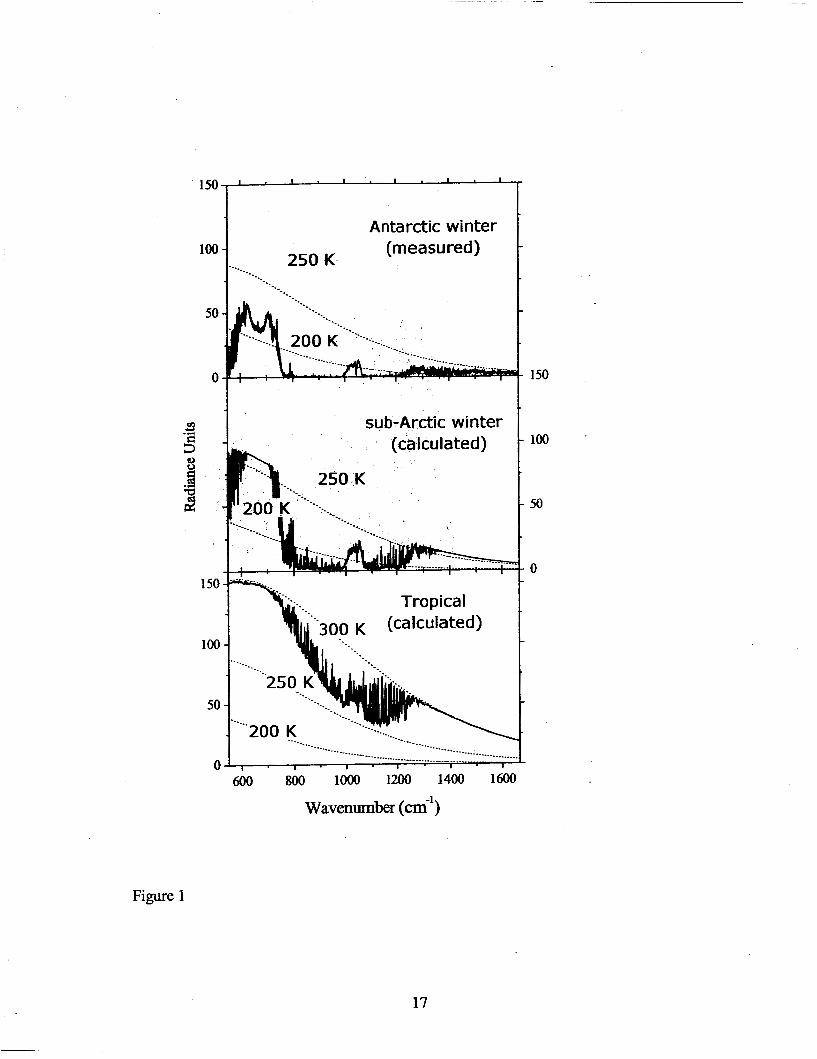
(Schwerdt&eger, 1970). Figure 1 shows the spectrum of downward longwave emission

from existing standard profiles compared with observations made at South Pole station;

the near-total lack of water vapor and the extreme cold over Antarctica produce a

radiance regime that is noticeably different even from conditions in the Arctic. Accurate

representations of the atmosphere over Antarctica, therefore, must derive fiom

observations made on the continent itself.

The development of an Antarctic standard atmosphere was greatly inhibited by

the extreme conditions of the Continent, as also by its remoteness. Whereas routine

weather observation programs in the more accessible and inhabited places often date back

more than a century, it was only in the International Geophysical Year (1957) that

monitoring programs over the Antarctic continent began (King and Turner, 1997).

Although these greatly added to our understanding of the continent, nearly all the stations

2

were - and are, even today - from the coastal Antarctic, and only a few stations were ever

operational on the high plateau. Of these, hundsen-Scott station at South Pole provides

the longest time series of data, with continuous observations dating back to the IGY

itself.

Fortunately, despite the isolated nature of South Pole station, observations from

this location may reasonably represent average conditions over much of the continent.

The surface elevation at the geographic pole is comparable to the average elevation over

the high plateau (see figure 2). Also, the high visible reflectance and infrared emissivity

of the snow surface makes representations of other contributions to the energy balance far

easier; conditions at the surface are largely determined by the longwave downward

radiance alone. The surface-based temperature inversion maintained by the radiative

balance exceeds 20 degrees over a few hundred meters of the lowest atmosphere for a

large portion of the plateau (Jeff Key, personal communication, 2003; Philpot and

Zillman, 1970). Recently, using a time series of annual mean temperatures for each pixel

in the 18-year satellite record over Antarctica, King (personal communication, 2003)

developed a method to determine the degree to which any given location is representative

of other locations in the continent. The correlation coefficient between the time series for

the South Pole and the time series at every other point (figure 3) shows that annual mean

temperature fluctuation at 90 S is representative of surface conditions over much of

plateau, with the exception of the highest elevations.

3

Temperature

Twice daily in summer (November-February) the South Pole Weather Office

(SPWO) conducts routine radiosonde launches; in winter the sondes are launched only

once each day. The temperature profiles obtained by these radiosondes include errors due

to the thermal lag of the thermistors; this problem is especially significant in atmospheric

layers where the lapse rate in very high - as in the surface based temperature inversion

over the Antarctic plateau. The values reported by the thermistor were corrected for this

lag thermal lag of thermistors on the radiosondes according to the method of Mahesh et

al. ( 1997). Using a 1 0-year period (1 993-2002) of observations, monthly average profiles

were constructed from radiosonde reports during each month, and multi-year averages of

such monthly profiles were crated. Averages were obtained as follows: temperatures

from each sounding were first inteqolated on to a 50-m grid. Following this, temperature

values at each height were averaged using all available soundings that reached that

height. The heights that soundings reach in the atmosphere vary considerably; at

stratospheric heights, therefore, fewer radiosondes are included in the average values than

at tropospheric elevations. For temperatures above 30 km (i.e. at atmospheric pressures

below 10 mb) we used monthly-average temperatures obtained by the Upper Atmosphere

Research Satellite @JARS) (Walden 1995). There is typically some overlap, as the

highest elevations reached by the sondes are often some kilometers higher than the lowest

elevation of UARS sounding. Mahesh (1999) observed that observations of atmospheric

radiance at the surface were better matched with calculations when UARS data fiom the

upper atmosphere was also included, but the radiances calculated were not particularly

4

sensitive to the temperatures at those elevations. Continuity between the somdmgs and

the UARS observations was therefore established by using the radiosonde data at the

overlapping elevations, md the UARS observations at higher levels.

Figure 4 shows the monthly average atmospheric profdes of temperature obtained

in this manner. The key features of Antarctic temperatures - the strong surface-based

inversion in the winter months, the extreme cold stratospheric temperatures at which

Polar Stratospheric Clouds form in the spring, the core-less minimum in surface

temperature throughout the winter - are all evident. There is also considerable variability

in upper-air temperature, but as noted earlier the contribution to the energy balance at the

surface from this portion of the atmosphere is small. The surface temperature, inversion

strength, stratospheric temperatures also suggest a basis for classification of the year-

round observations into seasonal profdes: Mar-April-May, June-July-August, September-

October-November, and December-January-February, as fall, winter, spring and summer

respectively. Temperature values for the individual months, as well as for these seasons,

are included in Tables 1 and 2; these may also be downloaded from httD://www.url-to-be-

decided(antkDrofiles.htm.

Ozone

Current research on high latitude climate change has emphasized the importance

of radiative and dynamic coupling between the troposphere and stratosphere, and the

impact of these interactions on the polarity of the Northern or Southern Annular Mode

(NAM or SAM; Shindell et al., 1999). Over Antarctica in particular, the springtime ozone

5

decrease in the stratosphere has been linked to a gradual strengthening of the SAM,

which may have driven a cooling of the continental interior and a warming of the

Antarctic Peninsula over the past two decades (comiso, 2000; Thompson and Solomon,

2002; Gillett and Thompson, 2003). A complete standard atmosphere of the Antarctic

Plateau must therefore accoullt for stratospheric ozone variability in order to be fully

applicable to climate studies.

The most important, and extreme, ozone variability is related to the anthropogenic

ozone decrease in the lower stratosphere from heterogeneous chemistry, that begins

during late winter and in recent years has lasted well into summer (Solomon, 1999). We

have therefore constructed model ozone profiles, from the surface through 50 km, as a

function of total column ozone amount in Dobson units (DU), for each of four seaso11s.

In contrast to the monthly variability in temperature and pressure profiles, the

climatological (pre-industrial) monthly variability in total column ozone is much smaller

than the variability due to the ozone "hole" and related dynamics of the stratospheric

polar vortex. However, there is enough seasonal variability in climatological ozone over

Antarctica that these variations should also be considered (Brasseur and Solomon, 1984).

Our objective is to provide a set of ozone profiles that allow the researcher to wnstmct a

realistic horizontal and vertical distribution in ozone abundance using readily available

satellite data from instruments such as the Total Ozone Mapping Spectrometer (TOMS).

Given a satellite measurement of total column ozone, the researcher can interpolate

between these standard ozone profiles at each altitude. In this way a climate model

6

simulation can be accurately initialized to accouflt for the large anthropogenic changes to

the ozone c o l m over Antarctica.

The model ozone profiles are based primarily on five years of electrochemical

concentration cell (Ea) ozonesonde data from the South Pole, collected by the NOAA

Climate Modeling and Diagnostics Laboratory (CMDL), kindly provided by Dr. J.

Hoffman. We analyzed 325 ozone profiles collected between January 1998 and January

2003. For each season, all ozone soundmgs that reached above 25 km were sorted into

total ozone column bins 10 DU wide. When there were fewer than three soundmgs in a

bin, adjacent bins were combined, resultmg in some bins as wide as 30 DU. In each bin,

the son- were averaged at each altitude grid point (0.25 km increments) and this

average was then smoothed from the surface to 30 km with a moving average over a 1

km altitude range. For the remaining -10-15% of the ozone column above 30 Inn, Solar

Backscatter Ultraviolet (SBUV) satellite ozone profiles were binned and averaged in a

similar fashion. Ten years of SBUV data were kindly provided by Dr. R. D. McPeters

(NASA Goddard Space Flight Center, personal communication, 2003). These matching

higher altitude profiles, for the closest season and total ozone column bins, were joined to

the tops of the appropriate sounding prome averages. Discontinuities between the two

profiles at 30-34 km were removed by smoothing if smaller than 2 x 10" and by

scaling the S B W profile to the sounding end point if larger than 2 x 10" ~ m - ~ . After

joining the sonde and SBUV profiles, the combined profde was smoothed a second time

with a moving 2 km average. This procedure for combining SBUV and sounding data is

adequate for constructing model ozone profiles whose primary applications include

7

climate and radiation budget studies in the troposphere and stratosphere. For applications

involving dynamics or chemistry of the upper stratosphere and mesosphere, the

researcher is advised to use SBUV data directly, which extend downward to 100 mb

(approximately 15 km over Antarctica). For climate studies, our ozone proNes are more

relevant than S B W data alone, because the sounding averages realistically specify ozone

abundances at the tropopause and in the lower stratosphere. The model ozone profdes

are tabulated online at h t t o : / / w w w . u i d ~ ~ ~ r o f i l ~ . h ~ as a function of

their total ozone column abundance in DU.

Examples of the model profiles from each season are shown in Figure 5. During

spring, we were fortunate to have CMDL sondes during the weak ozone "hole" of 2002,

and several of these showed climatologically normal ozone profiles with column

abundances greater than 330 DU. Thus our standard atmosphere is applicable to pre-

industrial climate modeling simulations. Most springtime ozone soundings, however,

showed some degree of anthropogenic ozone depletion, and the severest examples

(column abundances -100 DU> show a near total ozone loss between 15-20 km. During

the 199Os, the anthropogenic ozone decrease began to last into December, and the suite of

ozone profiles for s m e r includes one with total column abundance 154 DU. The ozone

profiles for autumn and winter show total column abundance variations that are mainly

climatological (e.g., Brasseur and Solomon, 1984), and the major differences here are

slightly larger ozone abundances (-30 DU) and a slightly thicker and higher stratospheric

ozone layer during autumn.

Water vapor

8

The measurement of water vapor over the high plateau has been severely impeded

by the lack of sensitivity of hygristors typically attached to radiosondes at the low

temperatures prevalent in the Antarctic atmosphere. This is made further difficult by the

fact that water vapor exists in such low quantities here; over much of the high plateau,

precipitable water vapor amounts are below 2 mm throughout the year. The spectral

signature from such low water vapor amounts (see infrared window between 8 and 12

microns in figure 1 ) is extremely small, even in COlTlparison to that from high latitudes in

the Arctic. Nonetheless, comparisons between measured downwelling longwave radiance

and calculations (Walden 1995) using theoretical profiles show that while minimal, water

vapor amounts cannot be set to zero, i.e., anecdotal knowledge of conditions on the

plateau can be used to provide reasonable representations of water vapor in standard

profiles, and these are adequate to mimic the gas’s measured radiative impact.

Even in clear-sky conditions it is common to find suspended ice-parties - known

as ‘diamond dust’ in the inversion layer just above the surface; this suggests that this

portion of the atmosphere is likely saturated with respect to ice. UARS data provide some

measurements of atmospheric water vapor in the middle and upper troposphere.

Radiosonde observations during and after cloudiness in the fiee troposphere (above the

inversion layer) suggest much greater variability of saturation levels here. And UARS

observations indicate only a few parts per million by volume (ppmv) of water vapor in

the upper troposphere. Following Walden (1 995) we recommend setting relative

humidity with respect to ice at 90% in the surface-based inversion layer, and at 75% at

elevations above the inversion but below 7 km. There is no sensitivity in radiative

9

calculations to values above this height; an efficient representation is to simply set water

vapor values to 5 ppmv at all heights above the tropopause.

Adjusting temperature for surface elevation

Several attriiutes of Antarctica - snow and ice cover, high elevation, latitude, etc.

- together allow representations of radiative Conditions over the continent to be made

more easily than ekewhere. However, there is one key attribute that impacts atmospheric

conditions, especially temperature, significantly - namely, the d a c e elevation. In figure

2, we observed that South Pole is most unlike the locations where surface elevation is

either substantially higher or lower, and much more representative of locations at similar

d a c e elevation. Observations of radiosonde data from the few stations where these are

available suggest that whereas lower tropospheric temperatures are markedly different

depending on surface elevation, upper troposphere temperatures are more comparable. In

particular in the lower troposphere, the inversion strength - the difference between

surface temperature and the warmest point of the lower troposphere - is much smaller on

the coast, and correspondingly the inversion height - the elevation of the warmest

location - is much greater. This variation is expect& when the surface elevation is at a

lower pressure, downward longwave emission from the atmosphere is radiatively

balanced by upward infrared emission by a colder surface, although d a c e conditions

themselves may be comparable in the two cases. This increases the inversion strength

with altitude, and correspondingly reduces the thickness of the layer over which the

radiative balance is established (this latter quantity is the inversion height).

10

This observation, while it is evident from the radiosonde data, is hadequate to

make strong correlations between surface elevations and inversion properties, because

nearly all of the radiosonde data is from coastal locations and the only long-period

observations other than these are from a single source (South Pole). Recently, however,

Liu and Key (2002, see figures 12 and 13) have developed a method of determining

inversion strengths and heights from clear-sky observations made by MODIS. Climate

modelers desirous of making more spatially detailed representations of lower

tropospheric temperatures can apply corrections based on relationships made from such

Conclusions

The need for standard atmospheric profiles of Antarctica that can be used in

climate models has been long-standing. It has especially been prompted by the

knowledge that not only is the atmosphere over the Antarctic plateau extreme, but

additionally, even in comparison to the Arctic winter atmospheres it is significantly

different. The extreme transparency of the infrared atmospheric window in Antarctica

also makes downward radiances in particular wavelength intervals highly sensitive to the

temperature profile. Mahesh et al. (1997) showed that temperature differences of only a

few degrees in the atmosphere below the inversion could produce a half percent change

in the downward longwave flux for clear sky in winter at the South Pole; this is

comparable to the effect caused by changes in carbon dioxide concentrations from pre-

industrial times to the present. Such sensitivity confirms that radiative transfer

11

calculations for the Antarctic atmosphere cannot be approximated by even the coldest

conditions elsewhere.

Clear sky fluxes at the top of the atmosphere as well as at the ground elevation of

South Pole (2835 meters) were calculated by the radiative transfer program STREAMER

(Key and Schweiger, 1998), using the standard Arctic winter profile, and again using a

typical Antarctic profile from this research. Fluxes at the top of the atmosphere and at the

surface differed by as much as 5-10 percent. These values are significantly greater thau

the magnitude of changes in fluxes expected from global warming over the next century;

to attempt to model Antarctic CondifioIlS using profiles taken elsewhere, therefore, would

sigruficantly undermine our ability to model the expected changes.

The standard profiles presented here primarily offer representations of

temperature and ozone concentrations in the atmosphere over the Antarctic plateah

whose understanding has been limited by lhe historical paucity of detailed observations.

Because the great majority of the area of the plateau is at a significant elevation, the

temperature correction for surface elevation is only significant near the edge of the ice

sheets. Ozone concentrations of different columnar amounts are shown for each season,

to account for the fact that the vertical distribution of ozone varies with season, even

when total column amomts are comparable. While water vapor amounts are extremely

low across much of the cuntinent, clearly this is not the case near the coasts; fortunately a

number of coastal stations are available from which routine observations can be obtained

wherever it is deemed that coastal values are more appropriate.

12

Acknowledgments

Contributions from both authors were supported by the Goddard Earth Science

and Technology program. We thank Prof. J. Hoffman for providing the ozonesonde data

and Dr. R. D. McPeters for providing the SBUV data.

13

\

References

Brasseur, G., and S. Solomon, 1984: Aeronomy of the Middle Atmosphere. D. Reidel,

Boston, 441 pp.

Comiso, J. C., 2000: Variability and trends in Antarctic surface temperatures from in situ

and satellite infrared measurements, .I Clim., 13,1674-1696..

Gillett, N., and D. F. W. Thompson, 2003: Simulation of recent Southern Hemisphere

Climate Change. Science, 302,273-275.

Key, J., and A. J. Schweiger, 1998: Tools for atmospheric radiative transfer: Streamer

and FlWNet. Computers and Geosciences, 24(5), 443-45 1.

King, J. C., and J. Turner, 1997: Antarctic Meteorology and Climatology. Cambridge

University Press, 40 West 20* Street, New York, Ny 1001 1-421 1, USA

Liu, Y. and J. Key, 2003: Detection and analysis of clear sky, low-level atmospheric

temperature inversions with MODIS, J. Amos. Ocean. Tech., 20,1727-1737.

Mahesh, A, 1999: Ground-based inpared remote sensing of cioudproperties over the

Antarctic plateau, Ph.D. thesis, University of Washington, Seattle WA 98 195.

Mahesh, A., V. P. Walden, and S. G. Warren, 1997: Radiosonde temperature

measuTemenfs in strong inversions: Correction for thermal lag based on an

expeIimmt at the South Pole. .I Atmos. and Oceanic Tech., 14: 45-53

McClatchey, R. A, R. W. Fenn, J. E. A. Selby, F. E. Volz, and J. S. Garing, 1972:Optical

Properties of the atmosphere. Rep. AFCRL-72-0497,108 pp. Available from

Geophysics Laboratory, Hanscom AFB, Bedford MA 0173 1.

Phillpot, H. R., and J. W. Zillman, 1970: The surface temperature inversion over the

Antarctic continent. J. Geoplzys. Res., 75,4161-69.

14

Schwerdtfeger, W. 1970: The Climate of the Antarctic. World Survq of Climtology 14,

253-355.

Shindell, D. T., R. L. Miller, G. A. Schmidt, and L. Pandolfo, 1999: Simulation of recent

northern winter climate trends by greenhouse-gas forcing. Nature, 399,45245.

Solomon, S., 1999: Stratospheric ozone depletion: a review of concepts and history. Rev.

Geophys., 37,275-3 19.

Thompson, D. W. J., and S. Solomon, 2002: Interpretation of recent Southern

Hemisphere climate change. Science, 296,895-899.Waldeq V. P., 1995: The

d o w a r d longwave radiation spectmm over the Antarctic plateau. Ph.D.

Thesis, University of Washington, Seattle, 267 pp.

15

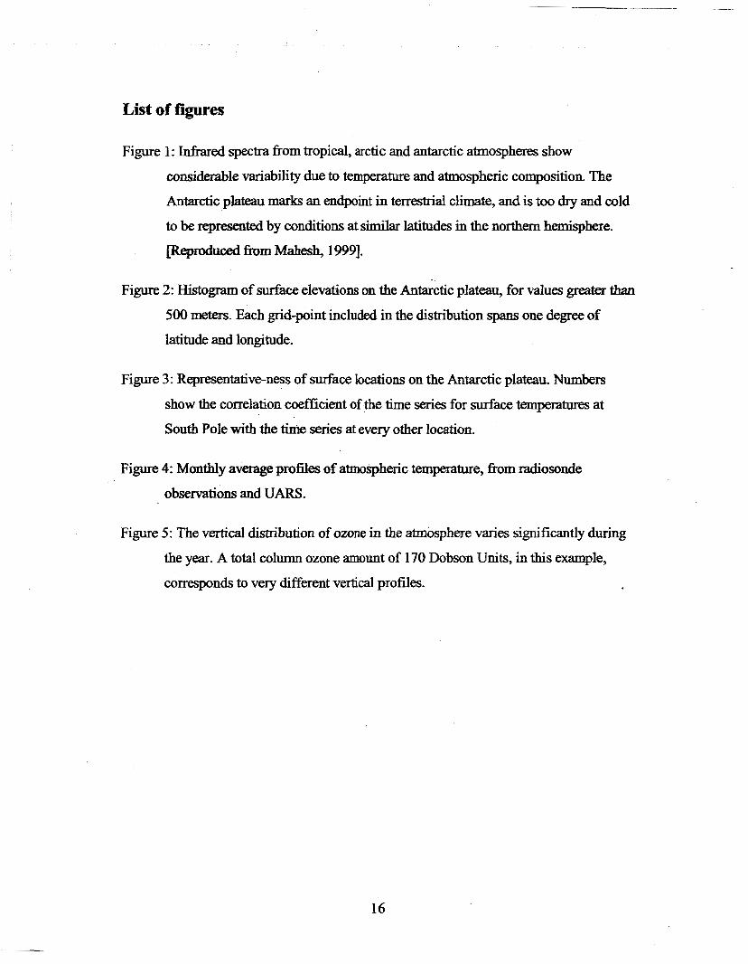
List of figures

Figure 1: Infi-ared spec,-a from -apical, arctic and antarcti atmospheres show

considerable variability due to temperature and atmospheric composition. The

Antarctic plateau marks an endpoint in terrestrial climate, and is too dry and cold

to be represented by conditions at similar latitudes in the northern hemisphere.

~eproduced from Maheh, 19991.

Figure 2: Histogram of surface elevations on the Antarctic plateau, for values greater than

500 meters. Each grid-point included in the distribution spans one degree of

latitude and longitude.

Figure 3 : Representative-ness of surface locations on the Antarctic plateau. Numbers show the correlation coefficient of the time series for surface temperatures at

South Pole with the time series at every other location.

Figure 4: Monthly average profiles of atmospheric temperature, from radiosonde

observations and UARS.

Figure 5: The vertical distribution of ozone in the atmosphere varies significantly during

the year. A total column ozone amount of 170 Dobson Units, in this example,

corresponds to very different vertical profiles.

16

Antarctic winter 100

50

0 150

100

50

0

Figure 1

17

100

I .w c 0 b

m 0

s

- E L

rc

50

E a r

c 1000 2000 3000 4000

surface elevation (m)

Figure 2

0-75 -0-75 -0-5 -025

Figure 3

19

60000

40000

L

0

so 40 40 -20 0 20 -I

L

:.Feb?.r

-80 -60 -40 -20 0 20

60000

40000

2oooo

0

60000

40000

Zoo00

0

Temperature CC)

Figure 4

20

Figure 5

21

POPULAR SUMMARY

A Standard Atmosphere of the Antarctic Plateau Ashwin Mahesh and Dan Lubin Submitted to the Journal of Climate, August 2004

Climate models often rely on standard atmospheres to represent various regions

because it is often computationally too difficult to include local representations from

every loation in the model. These standard profiles broadly capture the important

physical and radiative characteristics of regional atmospheres, and become benchmarks

for simulations by researchers. Such standards were made in the 1970s for most regions

of the planet, but not for Antarctica. This is a significant omission, because Antarctica

occupies a significant area (comparable to the United States) and is also very different

fiom any place on Earth. The standard profiles of other regions made for use in climate

models are not representative of Antarctica, and are therefore only of limited value as

substitutes in climate models. This research is an effort fill the void in the scientific

community’s library of standard atmospheres, so that future representations of the region

in climate models can be more accurate.

Using data from radiosondes, ozonesondes and satellite along with other

observations from South Pole station, typical seasonal atmospheric profiles for the high

plateau are compiled. Temperature profiles had to be corrected for measurement errors

caused by the slow response of the recording thermistors. Proper representations of

rapidly changing ozone concentrations (during the ozone hole) were also necessary,

because the same total column amounts of ozone in the atmosphere correspond to

different vertical distributions in different seasons. The effect of surface elevation on

tropospheric temperatures is also discussed; this is necessary because much of the high

plateau is at a very high elevation, and lower atmospheric temperatures are sharply

dependent on these heights. The differences between standard profiles developed here

and the most similar standard atmosphere that already exists - namely, the Arctic winter

profile - are calculated. These differences suggest that these new profiles will be

extremely usefid to make accurate representations of the atmosphere over the high

plateau.

The standard atmospheres developed here will be maintained online at both

NASA Goddard Space Flight Center and at the University of California, and fr-eely

available to the global community of climate modelers and researchers.