i vicUndt l

A STABILITY ANALYSIS OF THE RETAINING WALLS OF MACHU PICCHU

by

Melissa M. Fontanese, E.I.T.

BS in Civil Engineering, University of Pittsburgh, 2007

Submitted to the Graduate Faculty of

the Swanson School of Engineering in partial fulfillment

of the requirements for the degree of

Master of Science

University of Pittsburgh

2010

ii

UNIVERSITY OF PITTSBURGH

SWANSON SCHOOL OF ENGINEERING

This thesis was presented

by

Melissa M. Fontanese, E.I.T.

It was defended on

March 30, 2010

and approved by

Anthony T. Iannacchione, Associate Professor, Civil and Environmental Engineering

Luis E. Vallejo, Professor, Civil and Environmental Engineering

Julie M. Vandenbossche, P.E., Associate Professor, Civil and Environmental Engineering

Thesis Advisor: Luis E. Vallejo, Professor, Civil and Environmental Engineering

iii

Copyright © by Melissa M. Fontanese

2010

iv

The retaining walls of Machu Picchu, constructed of dry stacked granite blocks during the 15th

century, have remained standing for centuries in a challenging geologic and climatic setting with

little to no maintenance. In order to construct such enduring infrastructure, Incan engineers

understood the basic concepts that we use today to design modern retaining walls. A stability

analysis, based on conservatively selected parameters, reveals that the Incan walls generally meet

modern standards for sliding stability (assuming full-contact and thus maximum frictional forces

between blocks) and the walls nearly meet modern standards for overturning stability.

A fractal analysis of the walls, conducted by digitizing and analyzing photos of four

retaining walls and one dwelling wall, shows that the roughness of the stones making up the

walls is fractal. The analysis also shows that the size distributions of the stones in the walls are

fractal over several ranges, or multi-fractal.

The walls were simulated in the laboratory using a matrix of wooden dowels subjected to

normal loading via a direct shear apparatus. Force chains formed in the matrix; as the size

distribution of the dowels changed with the addition of multiple dowel sizes, the number of

dowels not engaged by force chains decreased until all of the dowels were engaged in

transmitting the load to neighboring dowels.

The fractal distribution of stone sizes in the walls aids in the transmission of load

between individual particles in the wall as demonstrated through the laboratory analysis of

A STABILITY ANALYSIS OF THE RETAINING WALLS OF MACHU PICCHU

Melissa M. Fontanese, E.I.T., M.S.

University of Pittsburgh, 2010

v

wooden dowels. By engaging each particle in sharing the loading, the full stability of the wall

can be realized.

vi

TABLE OF CONTENTS

PREFACE ................................................................................................................................... XV

1.0 INTRODUCTION ........................................................................................................ 1

1.1 BACKGROUND .................................................................................................. 1

1.2 OBJECTIVE ........................................................................................................ 4

2.0 RETAINING WALLS ................................................................................................. 5

2.1 STATE OF THE ART ......................................................................................... 6

2.1.1 Retaining Wall Design Methodologies ........................................................... 6

2.1.2 Drainage and Hydrostatic Pressure ............................................................... 8

2.1.3 Changes in Wall Type Preferences ................................................................ 8

2.1.4 Types of Retaining Walls ................................................................................ 9

2.1.4.1 Gravity and Semigravity Retaining Walls ........................................ 10

2.1.4.2 Cantilever Retaining Walls ................................................................ 14

2.1.4.3 Non-Gravity Cantilevered Walls ....................................................... 15

2.1.4.4 Mechanically Stabilized Retaining Walls ......................................... 18

2.1.4.5 Anchored Walls ................................................................................... 20

2.2 THE RETAINING WALLS OF MACHU PICCHU ..................................... 22

3.0 STABILITY ANALYSIS ........................................................................................... 25

3.1 MODERN RETAINING WALLS .................................................................... 25

vii

3.1.1 Sliding ............................................................................................................. 25

3.1.2 Overturning .................................................................................................... 27

3.1.3 Bearing Capacity ........................................................................................... 29

3.2 MACHU PICCHU’S RETAINING WALLS .................................................. 30

3.2.1 Sliding ............................................................................................................. 32

3.2.2 Overturning .................................................................................................... 35

3.2.3 Bearing Capacity ........................................................................................... 37

4.0 FRACTAL ANALYSIS OF INCAN WALLS ......................................................... 38

4.1 FRACTALS ........................................................................................................ 38

4.1.1 What is a Fractal?.......................................................................................... 38

4.1.2 Fractals and Roughness ................................................................................ 41

4.1.3 Fractals and Distribution/Fragmentation ................................................... 42

4.1.4 Fractal Behavior of the Retaining Walls at Machu Picchu ....................... 44

4.2 FORCE CHAINS ............................................................................................... 46

4.3 FRACTAL ANALYSIS OF THE WALLS AT MACHU PICCHU ............. 46

4.3.1 Fractal Analysis Using Digitized Photos ...................................................... 46

5.0 ANALYSIS AND RESULTS ..................................................................................... 57

5.1 ROUGHNESS OF THE INCAN WALLS ....................................................... 57

5.2 DISTRIBUTION/FRAGMENTATION OF THE INCAN WALLS ............. 62

5.3 FORCE CHAINS IN THE INCAN WALLS .................................................. 69

5.4 STABILITY ANALYSIS REVISITED ........................................................... 91

6.0 CONCLUSION ........................................................................................................... 92

APPENDIX A .............................................................................................................................. 95

viii

A.1 WALL 1 .............................................................................................................. 95

A.2 WALL 2 .............................................................................................................. 98

A.3 WALL 3 ........................................................................................................... 100

A.4 WALL 4 ........................................................................................................... 102

A.5 WALL 5 ............................................................................................................ 105

BIBLIOGRAPHY ..................................................................................................................... 107

ix

LIST OF TABLES

Table 1. Summary of sliding factors of safety for a monolithic sliding failure along the base of a particular block. ................................................................................................................ 35

Table 2. Summary of overturning factors of safety for a failure occurring at the base of the

particular block. ................................................................................................................ 37 Table 3. Values of DR and correlation coefficients for the walls ................................................. 60 Table 4. Values of DF and correlation coefficients for the walls. ................................................ 65 Table 5. Comparison of multi-fractal DF for all walls. ................................................................ 68 Table 6. Fractal Dimensions for laboratory Tests A, B, C, and D. .............................................. 90

x

LIST OF FIGURES

Figure 1. Map of Peru showing the location of Machu Picchu ...................................................... 2 Figure 2. Aerial view of Machu Picchu. Note the many retaining walls apparent along the

western slope of the site. ..................................................................................................... 3 Figure 3. A gravity wall made of stacked precast concrete blocks with keyways. ...................... 11 Figure 4. Schematic drawing of a gravity retaining wall .............................................................. 12 Figure 5. An example of a decorative concrete finish on a wall. (Photo property of

Boulderscape, Inc., and Soil Nail Launcher, Inc.) ............................................................ 13 Figure 6. Schematic drawing of an L-shaped cantilevered retaining wall ................................... 14 Figure 7. Schematic drawing of a non-gravity cantilever wall ..................................................... 16 Figure 8. A soldier beam and lagging wall supports a roadway and several buried water mains

along a stream in Sewickley, Pennsylvania, constructed via the top-down method. ........ 17 Figure 9. Schematic drawing of a mechanically stabilized earth wall ......................................... 18 Figure 10. Settlement may induce failures in mechanically stabilized earth walls. (Photo

property of J. Boward) ...................................................................................................... 19 Figure 11. Schematic drawing of an anchor wall with a tieback. ................................................ 20 Figure 12. Tiebacks used to strengthen a failing retaining wall in Pittsburgh, Pennsylvania.

(Photo property of J. Boward) .......................................................................................... 21 Figure 13. A cross-section of an agricultural terrace at Machu Picchu (Wright and Zegarra, 2000)

........................................................................................................................................... 23 Figure 14. Illustration of sliding failure. ...................................................................................... 26

xi

Figure 15. A "popout" failure in a gravity wall in Edgeworth, Pennsylvania. (Photo property of J. Boward) ......................................................................................................................... 27

Figure 16. Illustration of overturning failure. .............................................................................. 28 Figure 17. An overturning/toppling failure in a dry-stacked modular block wall. (Photo property

of J. Boward) ..................................................................................................................... 29 Figure 18. Illustration of bearing capacity failure. ...................................................................... 30 Figure 19. A simplified schematic drawing of the Incan walls used in the stability analysis. .... 31 Figure 20. Active pressure generated behind the wall in the stability analysis. .......................... 32 Figure 21. Illustration of a sliding "popout" failure. .................................................................... 33 Figure 22. Forces acting on a single sliding block in the model. ................................................. 34 Figure 23. Illustration of forces acting on an overturning block in the model. ........................... 36 Figure 24. Generation of the Koch Snowflake through four iterations. ...................................... 39 Figure 25. Trees are one example of a naturally-occurring fractal pattern. ................................. 40 Figure 26. Comparing an island (left) to a stone (right). ............................................................. 45 Figure 27. An island shown at two different scales. .................................................................... 45 Figure 28. Wall 1 (Photo property of L.E. Vallejo) ..................................................................... 47 Figure 29. Wall 2 (Photo property of L.E. Vallejo) ..................................................................... 48 Figure 30. Wall 3 (Photo property of L.E. Vallejo) ..................................................................... 49 Figure 31. Wall 4 (Photo property of L.E. Vallejo) ..................................................................... 50 Figure 32. Wall 5 (Photo property of L.E. Vallejo) ..................................................................... 51 Figure 33. Wall 1 - Digitized ....................................................................................................... 52 Figure 34. Wall 2 - Digitized ....................................................................................................... 53 Figure 35. Wall 3 - Digitized ....................................................................................................... 54 Figure 36. Wall 4 - Digitized ....................................................................................................... 55

xii

Figure 37. Wall 5 - Digitized ....................................................................................................... 56 Figure 38. Wall 1 – P vs. A .......................................................................................................... 58 Figure 39. Wall 2 – P vs. A .......................................................................................................... 58 Figure 40. Wall 3 – P vs. A .......................................................................................................... 59 Figure 41. Wall 4 – P vs. A .......................................................................................................... 59 Figure 42. Wall 5 - P vs. A ........................................................................................................... 60 Figure 43. Wall 1 - a vs. N(A>a) ................................................................................................. 62 Figure 44. Wall 2 - a vs. N(A>a) ................................................................................................. 63 Figure 45. Wall 3 - a vs. N(A>a) ................................................................................................. 63 Figure 46. Wall 4 - a vs. N(A>a) ................................................................................................. 64 Figure 47. Wall 5 - a vs. N(A>a) ................................................................................................. 64 Figure 48. Wall 1 – Multi-fractal dimensions .............................................................................. 66 Figure 49. Wall 2 - Multi-fractal dimensions .............................................................................. 66 Figure 50. Wall 3 - Multi-fractal dimensions .............................................................................. 67 Figure 51. Wall 4 - Multi-fractal dimensions .............................................................................. 67 Figure 52. Wall 5 - Multi-fractal dimensions .............................................................................. 68 Figure 53. Packing of uniform size stones (left) and packing of various sizes of stones (right). 69 Figure 54. Direct Shear Apparatus (Vallejo, 1991) .................................................................... 71 Figure 55. Arrangement of 67 seven-millimeter diameter dowels before applying 300-lb normal

load. ................................................................................................................................... 72 Figure 56. Resulting force chains formed with a 300-lb normal load applied to the seven-

millimeter dowels (six dowels were removed). ................................................................ 73 Figure 57. Arrangement of 64 seven-millimeter dowels and one nine-millimeter dowel before

applying ............................................................................................................................. 74

xiii

Figure 58. Resulting force chains formed with a 300-lb normal load applied to the seven-millimeter dowel matrix containing a single nine-millimeter dowel (three dowels were removed). .......................................................................................................................... 74

Figure 59. Arrangement of 60 seven-millimeter dowels and 3 nine-millimeter dowel before

applying ............................................................................................................................. 76 Figure 60. Resulting force chains formed with a 300-lb normal load applied to the seven-

millimeter dowel matrix containing 3 nine-millimeter dowels (three dowels were removed). .......................................................................................................................... 76

Figure 61. Test A –Arrangement of 164 five-millimeter irregular dowels before applying 400-lb

normal load. ...................................................................................................................... 77 Figure 62. The dowel matrix compresses an amount ∆H when load is applied to it. .................. 78 Figure 63. Test A – Arrangement of 164 five-millimeter diameter irregular dowels after

applying a 400-lb normal load, before reducing the load to 300 lbs. Note that no arches developed when 400 lbs was applied. ............................................................................... 80

Figure 64. Test A – Force chains developed after applying 300-lb normal load to the irregular

five-millimeter diameter dowels. ...................................................................................... 80 Figure 65. Test A – P vs. A .......................................................................................................... 81 Figure 66. Test A - a vs. N(A>a) ................................................................................................. 81 Figure 67. Test B – Arrangement of 159 five-millimeter irregular dowels with a single round

nine-millimeter dowel before applying 300-lb normal load. ............................................ 83 Figure 68. Test B – After applying the 300-lb normal load to the dowel matrix, no force chains

developed. ......................................................................................................................... 83 Figure 69. Test B – P vs. A .......................................................................................................... 84 Figure 70. Test B - a vs. N(A>a) ................................................................................................. 84 Figure 71. Test C – Arrangement of 159 irregular five-millimeter dowels with 3 nine-millimeter

dowels before applying a 300-lb normal load. .................................................................. 85 Figure 72. Test C – Arrangement of mixed shape dowels after applying 300-lb normal load. No

force chains developed. ..................................................................................................... 85 Figure 73. Test C – P vs. A .......................................................................................................... 86 Figure 74. Test C - a vs. N(A>a) ................................................................................................. 86

xiv

Figure 75. Arrangement of 153 irregular five-millimeter dowels with 3 nine-millimeter dowels and 5 seven-millimeter dowels before applying a 300-lb normal load. ............................ 87

Figure 76. Arrangement of dowels after applying 300-lb normal load – no force chains

developed. ......................................................................................................................... 88 Figure 77. Test D – P vs. A .......................................................................................................... 88 Figure 78. Test C - a vs. N(A>a) ................................................................................................. 89

xv

PREFACE

I would like to thank Dr. Vallejo for mentoring me throughout both my undergraduate

and graduate years and for introducing me to the impressive civil engineering achievements of

the Pre-Columbian world during my career at the University of Pittsburgh.

I would also like to thank my family, including my parents Blaine and Kimberly

Fontanese and my brother Richard, for your patience and encouragement. Thank youyou’re your

love and support and for encouraging me to pursue a career as an engineer - I couldn’t have done

it without you.

Thank you to the many mentors I’ve had so far throughout my career, including Steve

Geidel, Alicia Kavulic, Doug Beitko, and Joe Boward. Without their influence, I probably

wouldn’t even have given geotechnical engineering a second thought.

During my seven years at Pitt, I formed friendships with many amazing young engineers.

Thanks to all of you for everything you’ve done to help me through my academic and

professional careers, and above all for being great friends. Thanks to Kara Gamble and Kyra

Ceceris for listening to my rants and pretending to understand fractals and retaining walls. We

need to plan a trip to Machu Picchu!

Thank you to Dr. Vandenbossche and Dr. Iannacchione for taking the time to review my

thesis and sit on the committee, as well as for your support during my years at Pitt.

1

1.0 INTRODUCTION

1.1 BACKGROUND

The Inca Empire flourished during the 15th and 16th centuries in the Andes Mountains of

western South America. The Inca lacked a written language and the technology for the wheel

(Wright and Zegarra 2000), but they built extensive infrastructure throughout their territory in

the Andes. Roads and bridges to carry foot traffic, retaining walls to support agricultural terraces

and buildings, and engineered waterways for irrigation and wastewater were all critical,

engineered components of Machu Picchu (ABC-CLIO 2001), which is perhaps the best-known

ancient Incan city.

Machu Picchu is located on the eastern side of the Andes Mountains in what is now Peru,

east-southeast of Lima near the city of Cusco. Built for the Inca king Pachacuti, it was

constructed starting in the middle of the 15th century (ABC-CLIO 2001) on a mountaintop above

the Urubamba River. It was abandoned about a century after construction began, around the

time the Spanish conquistadors began to occupy South America. The ancient city lay forgotten

until Hiram Bingham rediscovered it in 1911 and subsequently published his photos of Machu

Picchu in National Geographic magazine (ABC-CLIO 2001).

2

Figure 1. Map of Peru showing the location of Machu Picchu

Pre-Columbian civilizations are sometimes thought to be primitive, inferior societies in

comparison to modern-day civilization. Some of the great achievements of pre-Columbian

societies have been credited to extra-terrestrial beings because they appear to be too advanced for

such “primitive” cultures to construct. In his book, Chariots of the Gods

These ancient structures have outlasted many of our modern structures without the

benefit of our rigorous mathematical design methods and modern building codes, while

demonstrating seemingly modern engineering concepts, such as modular wall construction and

, Erich Von Daniken

(1968) hypothesizes that our planet was visited by extra-terrestrial beings during ancient times.

Von Daniken surmises that these visitors were welcomed as gods (as the Spanish Conquistadors

were welcomed to the Americas) and many mysterious ancient sites around the world were

inspired by or perhaps even constructed by these alien visitors who come from a culture far more

advanced than that of our ancestors.

3

efficient drainage techniques. To this day, major soil movements are problematic in the Machu

Picchu region (V. Vilimek, 2006), sometimes so severe that the access route to Machu Picchu is

blocked. The Incas managed to build their city in such a way that, even while affected by a

multitude of geologic hazards, it remains standing centuries later.

Machu Picchu exemplifies the engineering expertise of pre-Columbian societies. In order

to facilitate agricultural activities and create a city high atop a steep mountain in the Andes, the

Inca had the ingenuity to construct terraces supported by stone retaining walls. The walls of

Machu Picchu have endured centuries of weathering, earthquakes, and various other naturally

degenerative processes on a steep mountainside with little to no maintenance. Over five hundred

years after construction, the walls are still standing.

Figure 2. Aerial view of Machu Picchu. Note the many retaining walls apparent along the western slope of the site.

N

4

Understanding the keys to the longevity of the Incan retaining walls will recognize the

intelligence of pre-Columbian societies and contribute knowledge that may improve design and

construction techniques for modern retaining walls.

1.2 OBJECTIVE

The objective of this thesis is to investigate the factors that have helped the retaining walls at

Machu Picchu to endure for so many centuries and explain some of the mechanisms that may

influence their long-term stability, such as: fractal characteristics; formation of force chains;

drainage characteristics; and durability of building materials.

This research focuses on comparison of the Incan walls to modern walls and construction

techniques, a generalized stability analysis of the Incan walls in accordance with modern

standards, fractal analysis using digitized photographs, and laboratory analogy using wooden

dowels in a direct shear apparatus to simulate the walls.

5

2.0 RETAINING WALLS

A retaining wall is a structure that holds back soil in order to facilitate a dramatic vertical

(or near-vertical) change in grade. Today, we often use retaining walls to mitigate existing

landslides, prevent future landslides, mitigate excessive erosion, support bridge approaches,

protect structures, and provide a greater “flat” surface for development. Modern retaining walls

fall into several broad categories, discussed in detail in Section 2.1.4, and are engineered to

standards specified by building codes to ensure their stability.

The Incas made extensive use of retaining walls at Machu Picchu. The Incan retaining

walls were constructed primarily to provide a relatively flat surface for construction of buildings,

roads, fountains, other infrastructure, and for agriculture. The Incas lacked a written language

and hence, their engineering works were not governed by written building codes as our modern

infrastructure is; however, even without the sophisticated knowledge we employ today, they

were able to construct an entire city that withstood centuries of neglect and is still standing to

this day.

6

2.1 STATE OF THE ART

2.1.1 Retaining Wall Design Methodologies

From a geotechnical standpoint, retaining walls are typically designed to an appropriate

factor of safety for bearing, sliding, and overturning. A factor of safety is defined as the ratio of

the sum of forces resisting failure to the sum of forces causing failure. The forces which

typically cause retaining wall failures include the lateral pressure imposed by the soil supported

by the wall, the weight of surcharge loads such as roadways or structures, and hydrostatic

pressure (described further in Section 2.1.2). Forces resisting failure of the retaining wall may

include the weight of the wall, the friction developed along the wall-soil interface, the passive

resistance generated by the soil in front of the wall, and the resistance generated by anchors or

other appurtenances, depending upon the type of retaining wall in question.

A factor of safety below 1.0 (the sum of the forces causing failure is greater than the sum

of the forces resisting failure) indicates failure of the structure and a factor of safety equal to 1.0

(the sum of the forces causing and resisting failure are equal) indicates a marginally stable

structure which is at equilibrium. At equilibrium, any small disturbance to this structure which

adds to the sum of forces causing failure will lead to failure of the structure.

Due in part to the marginal stability of a structure at a factor of safety of unity, retaining

walls and other structures are typically designed to a factor of safety greater than one, specified

by a building code or other local standard of care, in order to ensure the stability of the wall. By

including a factor of safety in the design process, the inherent variability in strength of

construction materials and the earth supporting and being retained by the wall is offset.

7

Structurally, the materials used to construct the retaining wall are typically checked for strength

and elastic deformation, at a minimum.

Several design methodologies have been employed in the design of retaining walls and

are selected based upon the local standard of care and type of retaining wall being designed. The

“state of the art” typically governs for the particular material type; traditionally steel retaining

walls were designed using allowable stress design (ASD) and concrete walls were designed

using ultimate strength or load factor design (LFD). Load and resistance factor design (LRFD) is

becoming increasingly popular for design (it is currently the state of the art for steel structures).

ASD compares the actual loads imposed on structural components to predetermined

allowable loads. These allowable loads are based on widely-accepted material strengths gleaned

from laboratory tests, to which a reduction factor is then applied thus providing a factor of safety.

Allowable loads/material strengths and appropriate factors of safety are governed by various

codes specific to the wall purpose and geographic/political regions.

While ASD applies a reduction factor to the strength of the material in question, LFD

applies a factor to the load on the structure. This factor increases the apparent magnitude of the

load, building the factor of safety into the load used for the design. As with other design

methodologies, the appropriate load factors and factors of safety are dictated by codes and the

local standard of care.

LRFD has become an increasingly popular design method in recent years and is preferred

in the realm of highway design. LRFD, a hybrid of the ASD and LFD methodologies, examines

a variety of limit states (reflecting the various conditions under which the structure must remain

stable). Load factors (greater than 1.0) are assigned to the loads imposed on the structure,

similar to LFD, and resistance factors (less than 1.0) are applied to the material properties of the

8

structure components, similar to ASD. Load and resistance factors are determined via statistical

analyses and are dictated by the applicable regulatory code.

2.1.2 Drainage and Hydrostatic Pressure

Functional drainage systems are critical to the long-term stability of retaining walls.

When water collects behind a retaining wall, it builds up excessive hydrostatic pressure behind

the wall and adds very large additional, often unanticipated (and thus unaccounted for during the

design process) loads to the wall. Hydrostatic pressure buildup can lead to catastrophic failures

of retaining walls.

To mitigate the buildup of hydrostatic pressure behind retaining walls, drains (backfilled

with a free-draining material) are usually located immediately behind the retaining wall and the

drained water is discharged via a weep hole in the face of the wall. Special care must be taken to

make sure that this water is diverted to an appropriate location; water ponding in front of a

retaining wall adjacent to a roadway can cause hydroplaning and ice hazards to motorists or may

lead to excessive softening of the subgrade and ultimately unanticipated settlement of nearby

structures.

2.1.3 Changes in Wall Type Preferences

As socioeconomic and materials science factors have changed, so has the preferred type of

retaining wall. Cost is one of the most important factors considered when determining the

appropriate type of wall for a specific project.

9

Historically, the cost of materials drove the cost of a civil engineering project. Labor was

plentiful and relatively inexpensive; construction materials required massive amounts of energy

to produce and were relatively expensive to manufacture. Many historic civil engineering

projects were focused on minimizing the amount of material required for construction and were

less focused on minimizing the labor required to build it. Cast-in-place walls, requiring very

little prefabrication and more on-site labor, were common due to the economic circumstances of

the time.

As labor movements advanced, the cost of labor rose; conversely, more efficient

automated manufacturing processes have decreased the cost of prefabricated construction

materials. Modular precast concrete walls have recently become increasingly popular as they

can both be inexpensively manufactured and require minimal labor to construct.

2.1.4 Types of Retaining Walls

Modern retaining walls can generally be classified as gravity/semigravity walls,

cantilever walls, non-gravity cantilever walls, anchored walls, and mechanically stabilized earth

walls. Retaining walls can be considered solely one of the aforementioned wall types or a hybrid

of multiple wall types.

A specific wall type is chosen for a particular project based on:

• the characteristics of the site soils and bedrock. Some walls are better suited to a

relatively shallow bedrock surface while others will perform just as well in a

thick soil mantle. Soft soils may induce bearing capacity and settlement

concerns. Very hard rock layers may make rock excavation (for particular types

of walls) impractical. Chemical characteristics of the soil may dictate that

10

specific materials be used to construct the retaining wall to mitigate corrosion

concerns.

• physical and spatial site constraints. The size and orientation of a site may dictate

the type of wall that will be constructed; some walls require relatively large

construction areas while others can be built in a relatively small area. The

location of overhead or buried utilities may dictate what type of wall may be

constructed – relocating utilities can be dangerous, inconvenient, and expensive;

it may be more cost-effective to choose a wall that can work around utilities

rather than relocating them.

• economic factors. Financial concerns often impose the majority of restrictions on

a project; not only does the owner wish to preserve the budget, he or she would

like the best product they can have for the lowest price possible.

• aesthetic considerations. The look of a wall is especially important when located

in an area where it will frequently be seen, for example: a wall supporting a

hillside behind a building; above a road; near a home; or in a scenic area. In

recent years, concrete has been used for many aesthetic touches – walls can be

made of colored and/or stamped concrete, mimicking a stone wall or rock cut.

2.1.4.1 Gravity and Semigravity Retaining Walls

Gravity walls are massive walls that utilize only their own weight in holding back soil.

The walls at Machu Picchu fall under the umbrella description of gravity walls. Gravity walls

are commonly constructed of dry stacked or mortared stones, precast concrete blocks, cast-in-

place concrete masses, or wire mesh gabions filled with stones, among other materials.

Semigravity retaining walls are made of reinforced concrete (steel reinforcing increases the

11

structural strength of the wall, reducing the required section). For the purpose of discussion

herein, semigravity walls will be considered a type of gravity wall.

Figure 3. A gravity wall made of stacked precast concrete blocks with keyways.

As previously discussed, proprietary “modular” walls have become popular in recent

years and are used for everything from backyard landscaping to roadway construction. Blocks

for modular walls come in a variety of sizes and finishes to suit both the engineering and

aesthetic requirements of the wall. They are sometimes held together with interlocking keyways

or dowels to provide some resistance to toppling failure. Machu Picchu’s retaining walls can be

considered modular walls in the sense that they are a large mass constructed of numerous

12

individual units, although they are not uniform, manufactured units like those of modern modular

walls.

Gravity walls are generally inexpensive relative to more complex retaining walls because

they can frequently be constructed without the use of sophisticated equipment and from fairly

common and easily procured construction materials; however, certain types of gravity retaining

walls, such as those made of wire mesh gabions filled with stones, can be fairly labor-intensive

to construct. As mentioned before, today’s construction projects tend to favor fast-paced

construction and minimal labor. As such, today’s projects favor modular, prefabricated units that

are uniform and easily assembled.

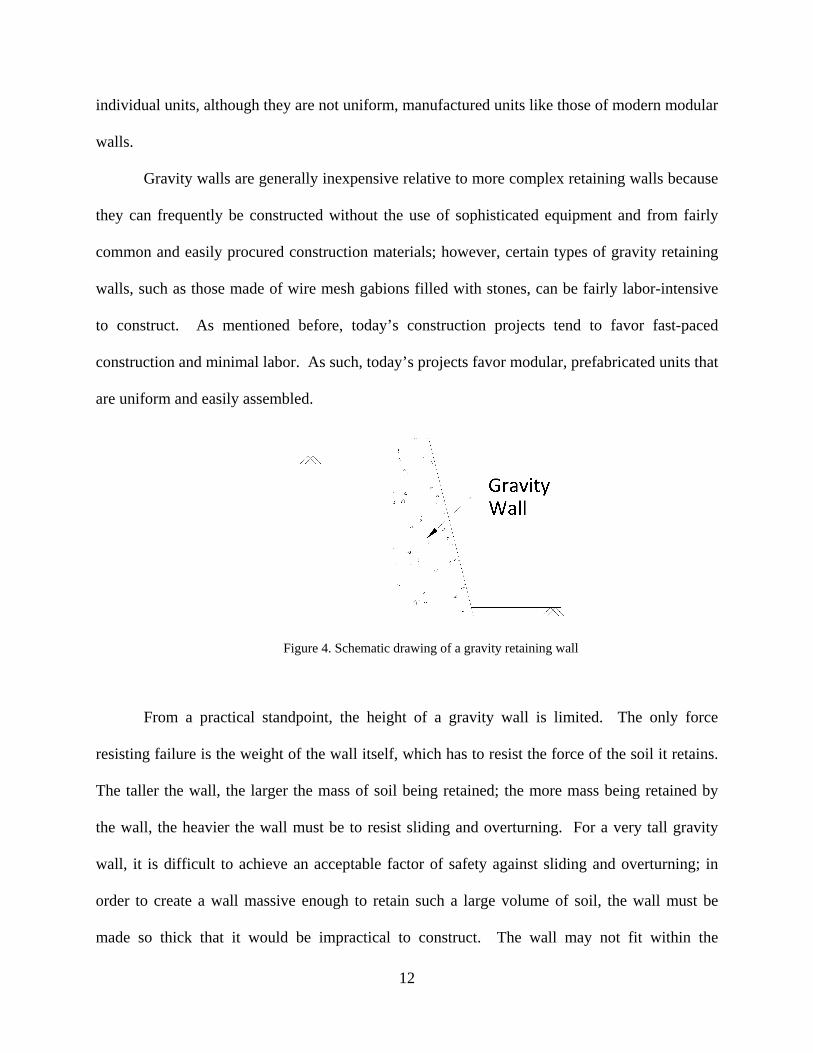
Figure 4. Schematic drawing of a gravity retaining wall

From a practical standpoint, the height of a gravity wall is limited. The only force

resisting failure is the weight of the wall itself, which has to resist the force of the soil it retains.

The taller the wall, the larger the mass of soil being retained; the more mass being retained by

the wall, the heavier the wall must be to resist sliding and overturning. For a very tall gravity

wall, it is difficult to achieve an acceptable factor of safety against sliding and overturning; in

order to create a wall massive enough to retain such a large volume of soil, the wall must be

made so thick that it would be impractical to construct. The wall may not fit within the

13

boundaries of the site or the volume of material required to produce a stable retaining wall may

be cost prohibitive. The weight of such a large retaining wall can lead to bearing capacity

failures and/or excessive settlements in the soil underlying the wall.

Most retaining walls built by homeowners are gravity walls. Homeowners generally

employ them to retain a yard superjacent to a depressed driveway, for decorative purposes in a

garden, or for other landscaping projects. They are relatively inexpensive for projects of such a

small magnitude and there are many contractors who are familiar with the appropriate

construction techniques; a homeowner may be able to construct a small modular wall on his own,

which can be a substantial cost savings over hiring a contractor to build it. Gravity walls can

easily be aesthetically pleasing – they may be made of stamped concrete which can be formed to

nearly any pattern the owner desires.

Figure 5. An example of a decorative concrete finish on a wall. (Photo property of Boulderscape, Inc., and

Soil Nail Launcher, Inc.)

14

2.1.4.2 Cantilever Retaining Walls

Cantilever walls resemble gravity walls, but with a cantilever arm added to the wall in

order to employ the weight of the retained soil in maintaining the stability of the retaining wall in

addition to the weight of the wall itself. Cantilevered walls are often shaped like an upside-down

“T” or “L”. Because of the added resistance from the cantilever, these walls usually require less

material than traditional gravity walls. They are typically made of cast-in-place, steel-reinforced

concrete.

Figure 6. Schematic drawing of an L-shaped cantilevered retaining wall

The cantilever arm gives this wall several advantages over a traditional gravity wall. The

weight of soil behind the retaining wall pushes down on the cantilever arm, creating a force that

resists overturning of the wall. The cantilever arm also increases the surface area of the base of

the wall, increasing the wall’s sliding resistance. From a functional standpoint, these additional

forces allow cantilever walls to function effectively over greater heights than traditional gravity

retaining walls. Cantilevered walls sometimes include counterforts (struts connecting the actual

wall to its cantilever arm) to reduce the required wall section. Thus, cantilever walls can

typically be made taller and more slender than their pure gravity wall counterparts.

15

In order to facilitate construction of the cantilever arm, a larger excavation is required

relative to that required for a traditional gravity wall. Depending upon the site geometry,

especially in instances where limited right-of-way or the location of a buried utility line is an

issue, additional excavation can be a deterrent when evaluating the suitability of a cantilever

wall. In order to provide a safe workspace, the excavation sidewall should be sloped back,

requiring even more space, or temporary shoring should be installed. Installing temporary

shoring is essentially building another wall just to facilitate the construction of the actual wall.

This may be deterrent due to its impacts on project finances and schedule.

In addition, the cantilevered wall is subject to the same practicality drawback as a

traditional gravity wall: beyond a certain height, the wall will have to be so massive that it may

be more cost- and space- effective to choose another wall type for the project.

2.1.4.3 Non-Gravity Cantilevered Walls

Non-gravity cantilevered walls are usually walls with continuous vertical elements (like

steel sheet piles) or walls with discrete vertical elements (like soldier beam and lagging walls).

Non-gravity cantilevered walls are constructed one of two ways: top-down or bottom-up. “Top-

down construction” implies that the wall is constructed from the top, down; in the case of a wall

on a slope, the wall can be constructed from the top of the slope, eliminating the need for

excavating a construction bench. Excavating a bench for bottom-up construction can be risky,

particular on a hillside, as the excavation may disturb the toe of the slope and possibly induce a

slope failure. A bench may also require temporary shoring, which will add additional cost to the

project. Top-down construction eliminates, or at the very least minimizes, the need for risky

and/or costly excavations. After constructing the wall, the soil in front of it can be excavated to

16

final planned grade; thus the retaining wall fills two roles: the role of temporary shoring for the

excavation and its intended role as a finished-product retaining wall.

Figure 7. Schematic drawing of a non-gravity cantilever wall

Sheet pile walls are constructed by driving sheet piling made of steel, wood, or vinyl into

the ground. Soldier beam and lagging walls are constructed by installing steel H-piles or wide-

flange beams spaced at a specified interval (by driving them into the ground or by drilling a shaft

and grouting them in place) and then installing concrete or wooden lagging between the piles.

The lagging retains the soil and is held in place by the steel piles. As a rule-of-thumb, non-

gravity cantilevered walls generally extend to depths of twice the exposed height of the wall

(Das, 2004). These walls are especially useful in “cut” situations because they can be installed

via the top-down method before the excavation takes place, eliminating the need for temporary

shoring during excavation.

17

Non-gravity cantilever walls are generally fairly expensive relative to gravity and

cantilever walls because construction frequently requires the use of expensive heavy machinery,

including cranes and large drill rigs. They are especially useful in areas with limited

construction space, such as a failing slope subjacent to a roadway, because they can be installed

via the top-down method. These walls have relatively small “footprints” and thus it is easier to

avoid conflicts with existing buried utilities during construction.

Figure 8. A soldier beam and lagging wall supports a roadway and several buried water mains along a stream in

Sewickley, Pennsylvania, constructed via the top-down method.

Aesthetically, both sheet pile walls and soldier beam and lagging walls can have a very

sterile, industrial appearance which may not be desirable for certain applications. In applications

where appearance is important, walls can be covered with an architectural veneer to give the

18

desired appearance. In the case of soldier pile and lagging walls, concrete lagging can be colored

and/or stamped to give a natural look or an artistic finish.

2.1.4.4 Mechanically Stabilized Retaining Walls

Mechanically stabilized earth walls are essentially specialized gravity walls which

employ strips of galvanized metal, geotextile, or similar manufactured mesh between compacted

lifts of soil faced with a skin (usually made of concrete). By reinforcing lifts of soil with

manufactured reinforcing strips or geofabrics, the soil’s shear strength is increased, and these

lifts work together as one large mass of soil. These walls are typically constructed with granular

rather than fine-grained soils for drainage purposes, thus reducing the risk of soil-weakening

excess pore water pressure buildup.

Figure 9. Schematic drawing of a mechanically stabilized earth wall

In addition to the typical design criteria of overturning, sliding, and bearing capacity (all

related to the external stability of the wall), mechanically stabilized earth walls must be checked

for internal stability. Internal stability for a mechanically stabilized earth wall relates to the

strength of the reinforcement (it should be designed to resist both pullout and tensile failures)

19

and the condition of the wall facing. The type of reinforcing used between layers of soil can

have a dramatic effect on the performance of the wall; metal strips, even when properly drained,

can be affected by oxygen and moisture in the soil and corrode, potentially leading to premature

failure of the structure.

Figure 10. Settlement may induce failures in mechanically stabilized earth walls. (Photo property of J. Boward)

A common mode of failure for mechanically stabilized earth walls is bearing capacity or

settlement. If the compacted soil is placed atop a weaker soil subgrade, the surcharge of the wall

may cause settlement in the subgrade and ultimately cause damage to the wall. If the lifts of soil

making up the wall are not properly compacted, the lifts may settle. Both of these types of

20

failures can cause distresses to the reinforcement and ultimately cause the wall to

catastrophically fail.

Whereas non-gravity cantilevered walls are best suited for “cut” situations, mechanically

stabilized earth walls are ideal for “fill” situations, such as highway embankments and bridge

approaches. These walls are especially useful in highway construction for fill embankments

where limited right-of-way does not permit the use of a slope.

2.1.4.5 Anchored Walls

Any type of retaining wall can be considered an anchored wall if additional support is

added to the wall by anchoring it back into the retained soil or into bedrock. Anchors increase

the capacity of the wall, thereby reducing the required section and allowing taller walls to be

constructed.

Figure 11. Schematic drawing of an anchor wall with a tieback.

Two general categories of anchors are employed in retaining wall construction: deadman

anchors and tiebacks. Deadmen are usually concrete blocks (precast or cast-in-place) attached to

21

the wall with a tie-rod or strut. Tie-rods/struts are attached to the face of the wall with a wale.

The deadman anchor works by gravity combined with the lateral passive pressures generated by

the soil in front of the anchor. Deadman anchors and their Rankine passive zones must be

located outside of the Rankine active zone behind the wall to realize the full resistance of the

anchor. Should the anchor be located completely within the active zone, the anchor will do

essentially nothing to assist the retaining wall in holding back the soil because it is located within

the wedge that is “moving along” with the wall as it moves.

Figure 12. Tiebacks used to strengthen a failing retaining wall in Pittsburgh, Pennsylvania. (Photo property of J.

Boward)

Tiebacks are steel cables or bars which are grouted in place. During construction, a hole

is pre-drilled to a specified depth, the steel is inserted into the borehole, and the borehole is then

pumped full of grout. The grout forms a grout bulb which serves to bond the steel tieback to the

22

soil or rock. Tiebacks may be tensioned during installation or tension may develop as load is

applied to the tiebacks.

Adding anchors to a non-gravity cantilevered wall can dramatically decrease the required

embedment depth and required section, saving on both materials and labor time; however,

installing anchors can be quite costly. They can make a geometrically impractical wall option a

more practical solution by reducing the required size of the wall. Anchors can sometimes be

used to “shore up” a failing retaining wall, as shown in Figure 12.

2.2 THE RETAINING WALLS OF MACHU PICCHU

The retaining walls found at Machu Picchu are gravity walls. The walls are constructed

of various sizes of stones, ranging from very massive stones (several feet in diameter) to smaller

stones (several inches in diameter). The Incas built solid foundations in the slope’s colluvial soil

from large stones or by building directly on top of exposed bedrock (Wright and Zegarra). The

walls of the agricultural terraces, studied herein, have a batter of approximately 5%. Several

layers of soil were used to backfill the walls: a base layer of gravel underlying a layer of fine

sand and gravel, capped with a topsoil layer used for growing crops. The stacked stones

continue below grade as a foundation system.

23

Figure 13. A cross-section of an agricultural terrace at Machu Picchu (Wright and Zegarra, 2000)

The Inca engineers understood the importance of effective drainage. The walls were

backfilled with layers of soil that increased in coarseness with depth to prevent the topsoil from

washing away (the change in gradation forms a sort of filter). The walls studied herein are dry

stacked walls that do not perfectly interlock – this allows excess water to weep out of the front of

the wall. Other nearly perfectly-interlocking walls were provided with weep holes, such as the

Artisans Wall (Wright and Zegarra). Drains constructed behind the walls were filled with rock

chips generated during stone cutting operations for the construction of the city. These drainage

measures reduce hydrostatic pressure buildup behind the walls and increase the long-term

stability of the city’s walls.

The retaining walls were constructed from granite blocks. Granite, a hard igneous rock,

is well-known for its durability and is used in a multitude of construction projects ranging from

24

the walls of Machu Picchu to architectural treatments for buildings to kitchen countertops. Had

the walls been constructed from sedimentary rocks, such as sandstone or siltstone, perhaps the

bonds cementing the individual particles in the rock together would have succumbed to the moist

climate of Machu Picchu long ago.

Of all the retaining walls at Machu Picchu, the agricultural terraces seem to have been

constructed with the least concern for aesthetics. Their stones were not carefully carved to

interlock like puzzle pieces or shaped into uniform blocks, but were irregularly shaped and of

greatly varied sizes. Perhaps the Incan engineers made a conscious decision to build walls in this

manner because they thought it would bring greater stability to the walls, or perhaps it was a

matter of convenience. Rather than taking the time and effort to perfectly carve each and every

stone, they could use “leftovers” from other projects or at the very least, minimize the

“fabrication time” - time spent quarrying and shaping stones - for the wall units. This variety of

shapes and sizes of individual stones may be one of the keys to the stability of the Incan walls,

along with effective drainage, and proper foundations. In Chapter 3.0, the stability of the walls

at Machu Picchu will be analyzed quantitatively.

25

3.0 STABILITY ANALYSIS

As discussed in Chapter 2.0, today’s retaining walls are generally designed to meet three

criteria: resistance to sliding, resistance to overturning, and adequate bearing capacity. This

chapter will further discuss each of these failure modes and use modern engineering analysis to

demonstrate the stability of the Incan retaining walls.

3.1 MODERN RETAINING WALLS

3.1.1 Sliding

A sliding failure occurs when the horizontal forces pushing against the retaining wall overcome

the horizontal forces holding the retaining wall in place and the wall is displaced forward along

the ground surface. In dry stacked walls, individual wall units may slide with respect to one

another (a “popout”-type failure) and cause a portion of the wall to fail.

The factor of safety against sliding along the base of a retaining wall is defined by the

ratio of the forces resisting sliding to the forces driving sliding and can be expressed as

(Equation 3.1)

26

A factor of safety against sliding equal to 1.5 is commonly used in design.

Figure 14. Illustration of sliding failure.

The force causing sliding in the case of the Incan walls (and other gravity walls) is the

horizontal pressure exerted by the soil and water pressure behind the wall. The resisting forces

include friction between the base of the wall and the soil, and the passive pressure generated by

the soil in front of the toe of the wall. Mechanically stabilized earth walls, like gravity walls,

achieve their resistance to sliding via the friction generated along the base of the wall. In the

case of cantilevered retaining walls, additional frictional resistance is achieved by the greater

surface area of the base of the wall (relative to traditional gravity walls. Non-gravity

cantilevered walls overcome sliding failure by amassing a large quantity of passive earth

pressure in front of the wall. Anchored walls achieve greater sliding resistance via horizontal

forces generated by the anchors, in addition to friction along the base of the wall and/or passive

pressure generated by the soil in front of the wall.

27

Figure 15. A "popout" failure in a gravity wall in Edgeworth, Pennsylvania. (Photo property of J. Boward)

3.1.2 Overturning

Overturning failure occurs when the forces pushing against the wall cause it to rotate about its

toe, tipping it over. Smaller-scale toppling failures tend to occur in modular dry-stacked walls,

whereby the individual units making up the wall may overturn, causing just a portion of the wall

to fail.

28

Figure 16. Illustration of overturning failure.

The factor of safety against overturning is calculated by the ratio of the moments about

the toe of the wall tending to resist overturning to the moments about the same point driving

overturning and can be expressed as

(Equation 3.2)

In practice, a factor of safety of 2 to 3 is commonly applied to resist overturning (Das, 2004).

In the case of the walls at Machu Picchu, the moment resisting overturning is generated

by the weight of the wall itself. Resistance to toppling failures of individual units in the wall

comes from the weight of the individual stones. The overturning moment is generated by the

horizontal force of the soil and water behind the wall.

The forces generated by the weight of the wall and the lateral pressure from the soil are

the forces at work in overturning today’s state of the art retaining walls, as well. In the case of

non-gravity cantilevered walls, the passive pressure generated in front of the wall also

29

contributes to the resisting moment; for anchored walls, the anchor contributes a portion of the

resisting moment, too.

Figure 17. An overturning/toppling failure in a dry-stacked modular block wall. (Photo property of J. Boward)

3.1.3 Bearing Capacity

A wall’s foundation subgrade must be checked for bearing capacity to be certain that the bearing

capacity of the subgrade is sufficient to withstand the force exerted upon it by the retaining wall.

The factor of safety for bearing capacity is the ratio of the ultimate bearing capacity of the soil to

the pressure exerted at the base of the retaining wall’s foundation. A factor of safety for bearing

capacity equal to 3 is commonly used in practice (Das, 2004).

30

Figure 18. Illustration of bearing capacity failure.

3.2 MACHU PICCHU’S RETAINING WALLS

This section presents the results of a stability analysis of the retaining walls at Machu Picchu,

including a simplified analysis to determine the walls’ factor of safety against sliding and

overturning.

The model used for the stability analysis is based on conservative information gleaned

from published resources and assumed information. Because excavations are very rarely

permitted at Machu Picchu, little is known about the backfill and foundation of the walls.

In the stability model, shown in Figure 19, the walls are seven feet high, made up of

vertically-stacked granite blocks measuring one foot high by one foot wide by two and one-half

feet deep. The angle of friction between the granite blocks is assumed to be 35 degrees and the

unit weight of the blocks is assumed to be 160 pounds per cubic foot (Hoek and Bray, 1981).

31

As shown in Figure 13, the wall extends below grade at the front of the wall such that the wall

analyzed herein sits atop a granite block.

The backfill is assumed to be a well-drained sand with no cohesion, an internal friction,

φ, of 30 degrees, and a unit weight of 110 pounds per cubic foot, although Wright and Zegarra

indicate that the backfill of the agricultural terraces is composed of several different layers, as

shown in Figure 13. The simplified model used for this analysis assumes a single layer of

backfill extending the entire height of the wall (rather than three distinct soil layers).

Figure 19. A simplified schematic drawing of the Incan walls used in the stability analysis.

The pressure generated behind the wall was calculated using Rankine theory. The

backfill generated a pressure of 257 pounds per square foot, as indicated in Figure 20. No

32

hydrostatic pressure was included in this analysis; the Incan walls are well-drained, as indicated

by Wright and Zegarra, so no hydrostatic pressure builds behind the walls.

Figure 20. Active pressure generated behind the wall in the stability analysis.

3.2.1 Sliding

Two different sliding failure modes are possible in dry-stacked walls such as the model wall.

The stones can slide with respect to one another (a “popout”-type failure where one block is

pushed out from between two others), as illustrated in Figure 21, or the entire wall may slide

with respect to the ground surface as if it were one monolithic unit, as shown in Figure 14. Both

of these cases were evaluated for this stability analysis. Each case was also checked for seismic

conditions, assuming a seismic coefficient of 0.15.

33

Figure 21. Illustration of a sliding "popout" failure.

In the case of stones sliding with respect to each other, three forces, shown in Figure 22,

were at play: the force generated by the active pressure behind the particular stone; the friction

force generated between the stone and its upper neighbor; and the friction force generated

between the stone its lower neighbor. No passive earth pressure-generated forces are at work in

this analysis as the wall does not truly extend below the ground surface. The factor of safety for

each of the seven blocks making up the wall was calculated to be 12.5, and in the case of an

earthquake, 10.8. Thus, when considering the stability of individual blocks with respect to one

another, the retaining walls at Machu Picchu far exceed the typical modern minimum factor of

safety against sliding.

The model wall was also analyzed for a monolithic sliding failure, assuming that the

entire wall above a particular block slid forward along the base of that block. In this case, only

two forces were at work: the force generated by the active soil pressure behind the wall and the

friction force generated along the base of the block in question. Again, no passive earth pressure

is generated in front of the wall. The calculated factors of safety are summarized in Table 1.

34

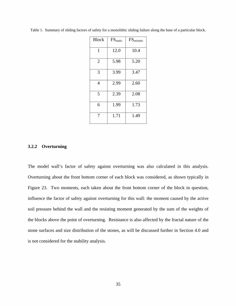
The factor of safety against sliding tends to decrease as the height of the failure increases,

ranging from 12.0 (in a static situation with only the top block sliding) to 1.49 (in the case of an

earthquake and all seven granite blocks sliding together). Again, these factors of safety are

greater than or approximately equal to 1.5, usually the minimum factor of safety used in design

today.

Figure 22. Forces acting on a single sliding block in the model.

Wright and Zegarra indicate that some of the walls were designed such that the individual

stones have “top or bottom indentations that help them fit together in a nesting manner.” While

these indentations are not considered in this simplified stability analysis, it should increase the

stability of the walls by contributing a greater resisting force, in addition to the friction force. As

shown later in Section 5.1, the stones have a structural roughness which also contributes to the

“interlocking” between individual wall units.

35

Table 1. Summary of sliding factors of safety for a monolithic sliding failure along the base of a particular block.

Block FSstatic FSseismic

1 12.0 10.4

2 5.98 5.20

3 3.99 3.47

4 2.99 2.60

5 2.39 2.08

6 1.99 1.73

7 1.71 1.49

3.2.2 Overturning

The model wall’s factor of safety against overturning was also calculated in this analysis.

Overturning about the front bottom corner of each block was considered, as shown typically in

Figure 23. Two moments, each taken about the front bottom corner of the block in question,

influence the factor of safety against overturning for this wall: the moment caused by the active

soil pressure behind the wall and the resisting moment generated by the sum of the weights of

the blocks above the point of overturning. Resistance is also affected by the fractal nature of the

stone surfaces and size distribution of the stones, as will be discussed further in Section 4.0 and

is not considered for the stability analysis.

36

Figure 23. Illustration of forces acting on an overturning block in the model.

The factors of safety determined in this analysis and summarized above in Table 2,

decreased with increasing wall height and ranged from 1.67 to 81.1. While the minimum factor

of safety determined in this analysis, 1.67, is not as great as the typical modern-day factor of

safety ranging from two to three, it is still greater than unity, indicating that the wall is indeed

stable. Due to the generalized nature of this assessment, in reality the factor of safety for the

Incan walls likely varies from the factors of safety determined herein.

37

Table 2. Summary of overturning factors of safety for a failure occurring at the base of the particular block.

Block FSoverturning

1 81.8

2 20.5

3 9.01

4 5.11

5 3.27

6 2.27

7 1.67

3.2.3 Bearing Capacity

Although not quantitatively analyzed herein, Machu Picchu’s retaining walls foundations appear

to be adequately designed for bearing capacity. According to Wright and Zegarra, “to create a

firm bedding,” the Incas placed smaller stones in the bottom of the excavation where the walls

were founded in soil and in the case of some much larger retaining walls, used very large stones

for the foundation (or even built directly atop bedrock where possible).

38

4.0 FRACTAL ANALYSIS OF INCAN WALLS

4.1 FRACTALS

4.1.1 What is a Fractal?

In mathematicians’ attempts to describe natural phenomena, difficult-to-describe natural

objects are usually reduced to well-defined objects from Euclidean geometry. Planets can be

seen as spheres, a blade of grass can be seen as a triangle, a mountain can be seen as a cone.

Benoit Mandelbrot, often considered the father of fractal geometry, cautioned that “mountains

are not cones, clouds are not spheres.” Mandelbrot brought together many previously discovered

mathematical peculiarities under the banner of “fractals” to describe these natural occurrences.

Fractals have been used to describe many irregular and seemingly random phenomena

that cannot be fully explained with classical mathematical concepts: snowflakes; Brownian

motion; coastlines; and other natural occurrences/processes. The topological dimension of an

object comes from Euclidian geometry; a ball, a veil, and a thread can be modeled to be three-,

two-, and one-dimensional, respectively (Mandelbrot, 1977).

Benoit Mandelbrot coined the term “fractal” in 1975 and defines it as “a set for which the

Hausdorff-Betiscovitch dimension strictly exceeds the topological dimension,” (Mandelbrot,

1977). Mandelbrot calls the Hausdorff-Betiscovitch dimension “the fractal dimension,” denoted

39

as “D” because this dimension is often fractional (Baveye and Boast, 1998). Mandelbrot (1977)

states that, “For every set S, there exists a real value D such that the d-measure [the topological

dimension] is infinite for d < D and vanishes for d > D.” This D is the Hausdorff-Besicovitch

dimension and the fractal dimension.

In a theoretical sense, fractals are part of a family of “mathematical monsters.” These

monster curves were discovered centuries ago by mathematicians (Baveye and Boast, 1998). An

iterative approach is used to construct visual representations of the monster curves. An initiator

(an equilateral triangle - three straight line segments - for the case of the Koch Snowflake, as

shown in Figure 24) is drawn and then modified by a generator (in this case, a symmetrical peak

constructed of two horizontal line segments and two angled line segments). The monster curve’s

construction is progressed by replacing each initiator with a generator, creating an increasingly

complex shape. With each iteration, the curve begins to look more and more like a snowflake, as

shown in Figure 24. As these monster curves were further developed over the years, they led to

the visually stunning computer-generated “fractals” we see today.

A fractal can be described visually as something that is self-similar and scaling. Fractals

are roughly identical at any scale, small or large (Mandelbrot, 1982); for example, the Koch

Snowflake pictured above shows an equilateral triangle at four different scales (the triangle

Figure 24. Generation of the Koch Snowflake through four iterations.

40

becomes smaller with each iteration). A tree can be considered fractal. Looking at an entire tree

is roughly the same as looking at one branch of that tree but with a different scale. They each

have a main stem (the trunk in the case of a whole tree or a limb in the case of the branch).

Smaller limbs, branches, and twigs split off from the main stem. From these smaller limbs, even

smaller limbs divide, and so on. As one zooms into the tree, one sees the same general pattern as

that displayed by the entire tree, as shown in Figure 25. This concept can be applied to many

natural objects: consider a fern, a head of cauliflower, a mountain, a network of rivers and

streams, or the human circulatory system; they are all fractals.

Figure 25. Trees are one example of a naturally-occurring fractal pattern.

41

4.1.2 Fractals and Roughness

Hyslip and Vallejo (1997) showed that the roughness of a population of fractal shapes

can be quantified using the area-perimeter method. The linear extent of a geometric pattern can

be represented by its perimeter (P), the square-root of its area (A1/2), or the cube-root of its

volume (V1/3). The ratio of any two of a pattern’s linear extents gives a constant that is specific

to that pattern. Consider a circle with a radius, r:

(Equation 4.1)

(Equation 4.2)

Taking the ratio of the linear extents of the circle gives:

(Equation 4.3)

It can be seen that for any circle, the relationship in Equation 4.3 holds true. The ratio of the

linear extents for other geometric patterns yields the pattern’s unique constant.

A quantitative measure of a geometrically similar population of fractal shapes can be

obtained through the ratio of linear extents for that population (Mandelbrot, 1983 as cited by

Hyslip and Vallejo, 1997). Mandelbrot proposed that the “ratio of linear extents” is fractal for

fractal patterns and proposed that:

42

(Equation 4.4)

where c is a constant and DR is the value of the roughness fractal dimension for the population of

fractal patterns. A log-log plot of P vs. A for each individual object in the population yields a

straight line with a slope, m, related to the fractal dimension by:

(Equation 4.5)

This type of analysis, the area-perimeter method, quantifies the roughness of a population

of similar geometric patterns. The roughness quantity can be representative of either the

structural or the textural characteristics of the population, depending on the level of scrutiny

(Hyslip and Vallejo, 1997). At a low resolution, an object’s general structure is quantified; at a

high resolution, an object’s textural characteristics are quantified.

4.1.3 Fractals and Distribution/Fragmentation

Populations exhibiting fractal characteristics, commonly called probabilistic fractals, can

exhibit a power law relationship as a result of their fractal geometry (Baveye and Boast, 1998).

The Pareto or power law distribution, originally illustrating the distribution of income in a

population, is given by the equation:

(Equation 4.6)

where N is the number of persons having income ≥ x. Plotting N as a function of x results in a

distribution with a long right tail.

43

This concept can be extended to perimeter-area plots. As demonstrated in Korvin (1992),

J. Korcak (1940) found during his analysis of the perimeter and area of islands that the

distribution of a population geographic objects follows a pareto distribution and proposed the

following equation, Kocak’s Law, where k and b are constants and A represents area:

(Equation 4.7)

Mandelbrot, realizing that this distribution was a result of fractal fragmentation, applied

Korcak’s Law to fractals. He suggested that b in Equation 4.7 is equal to the fragmentation

fractal dimension, DF, and developed the following equation:

(Equation 4.8)

Where N(R>r) is the total number of particles with a linear dimension R greater than a given size

r and k is a constant as in Equation 4.7. A log-log plot of N(R>r) will genearate a straight line

with a slope m where:

(Equation 4.9)

Equations 4.8 and 4.9 are based on the linear dimension of an object (radius, perimeter, diameter,

etc.). Relating these relationships to area, whose linear extent is the square-root of area, gives:

(Equation 4.10)

44

(Equation 4.11)

Thus, a log-log plot of N(A>a) vs. a will generate a straight line with a slope equal to -DF/2.

It should be noted that DF differs from the previously described DR and is not

representative of the roughness or shape of a specific population of objects, but rather a measure

of the distribution of that population’s specific traits (area, in the case of Equations 4.10 and

4.11).

4.1.4 Fractal Behavior of the Retaining Walls at Machu Picchu

In his 1977 publication’s chapter entitled “How Long Is the Coast of Britain?”

Mandelbrot describes how the concept of fractals and the fractal dimension can be applied to

coastlines and islands. The rocks that make up the retaining walls at Machu Picchu are

analogous to islands. By visualizing the walls as two-dimensional (when viewing the front face

of the wall), the irregular outline of the individual rock faces can be equated to that of an island,

as shown in Figure 26.

The coastline of an island and the perimeter of a rock face demonstrate fractal properties.

At any scale, one can see the boundary between the object and its surroundings: water in the case

of an island, and the other stones in the case of the retaining walls. As one zooms in closer on

the object’s boundary line (demonstrated in Figure 27), more and more asperities become visible,

and the boundary line is just as chaotic as it was when observing the entire object. This erratic

boundary line cannot be easily described by Euclidean geometry; but the self-similar, scaling

behavior of the boundary line can be described as a fractal. Not only are the boundaries of the

45

individual stones fractal, but the size distribution of the stones forming each wall has a fractal

dimension, as discussed in Section 5.2.

Figure 26. Comparing an island (left) to a stone (right).

Figure 27. An island shown at two different scales.

46

4.2 FORCE CHAINS

Vallejo et al. (2005) investigated the crushing of granular materials and found that granular

materials, when subjected to various loads, form force chains through which the load is carried.

Force chains form when the applied load is passed through the contacts between granular

materials. Using the discrete element method in a computer model, they found that the size

(thickness) of the force chains varied proportionately to the applied load and that the distribution

of force chains in the matrix is fractal.

The retaining walls at Machu Picchu may be considered analogous to the model used by

Vallejo. The walls are a matrix of granular particles (albeit on a much larger scale than that

investigated by Vallejo) subjected to vertical loads imposed the particles’ self weight.

4.3 FRACTAL ANALYSIS OF THE WALLS AT MACHU PICCHU

4.3.1 Fractal Analysis Using Digitized Photos

Figure 33 through Figure 37 are photos, taken by L.E. Vallejo in 2007, showing the five walls

subject to analysis in this study. Figure 33 through Figure 36 show four retaining walls, while

Figure 37 shows a stone dwelling wall at Machu Picchu.

47

Figure 28. Wall 1 (Photo property of L.E. Vallejo)

48

Figure 29. Wall 2 (Photo property of L.E. Vallejo)

49

Figure 30. Wall 3 (Photo property of L.E. Vallejo)

50

Figure 31. Wall 4 (Photo property of L.E. Vallejo)

51

These five photos were digitized, as shown below in Figure 33 through Figure 37, using

AutoCAD 2007 software by AutoDesk, Inc., on a personal computer. Each individual stone

making up the walls was outlined by visual estimation of the boundary and modeled as a polygon

in the program. The area and perimeter of each individual polygon representing a rock face were

determined by the software and recorded for use in the fractal analysis, as discussed in Chapter

5.0.

Figure 32. Wall 5 (Photo property of L.E. Vallejo)

52

Figure 33. Wall 1 - Digitized

53

Figure 34. Wall 2 - Digitized

54

Figure 35. Wall 3 - Digitized

55

Figure 36. Wall 4 - Digitized

56

Figure 37. Wall 5 - Digitized

57

5.0 ANALYSIS AND RESULTS

5.1 ROUGHNESS OF THE INCAN WALLS

Each of the five wall photographs were digitized and analyzed as described in Chapter 4.0. For

each wall, the corresponding perimeter (P) and area (A) for each individual stone making up the

particular wall were plotted on a log-log graph, employing the relationships introduced in

Section 4.1. Stones along the “perimeter” of the photo were eliminated from the analysis for the

four retaining walls and the middle one-third of stones making up the house wall were examined,

as many of the stones along the edges of the photo were cut-off by the camera and were not

representative of the actual size and dimension of the stones making up the wall. Least squares

linear regression was used to determine the line of best fit through all of the remaining data

points. Figure 38 through Figure 42 show the five perimeter-area (P vs. A) plots generated for

the walls.

58

Figure 38. Wall 1 – P vs. A

Figure 39. Wall 2 – P vs. A

59

Figure 40. Wall 3 – P vs. A

Figure 41. Wall 4 – P vs. A

60

Figure 42. Wall 5 - P vs. A

Table 3. Values of DR and correlation coefficients for the walls

DR R2

Wall 1 1.07 0.950

Wall 2 0.970 0.988

Wall 3 0.965 0.980

Wall 4 0.993 0.985

Wall 5 0.975 0.942

As shown by the P vs. A plots above, the data fits a power-law distribution as discussed in

Chapter 4.1.2, with a correlation coefficient ranging from 0.942 to 0.988. The roughness fractal

dimension for the five walls examined in this study ranged from 0.965 to 1.07. The average

fractal roughness dimension for the walls is 0.995. The range in roughness for the walls

61

indicates that the stones making up Wall 3 are the smoothest, while those making up Wall 1 are

the roughest.

Wall 2, Wall 3, Wall 4, and Wall 5 all appear to have a roughness dimension less than

one based upon the results of the least squares regression analysis. In fractal geometry, as in

Euclidean geometry, a dimension equal to zero represents a single point and a dimension of unity

represents a solid line. A dimension between zero and unity, possible in the realm of fractal

geometry, represents a broken line. Thus, the minimum dimension of any of the stones making

up the walls at Machu Picchu should be one (they are each represented by an unbroken line

encompassing the area of the stone). Although the perimeters of all of the rocks modeled in this

analysis are actually solid lines, due to the fact that the line of best fit generated by the least

squares regression analysis depends upon values of the entire population, the slope of the line of

best fit can be skewed to give a misleading roughness dimension.

Because the level of scrutiny of the stones’ perimeters is relatively low (a low level of

magnification was used to determine the perimeter), the roughness dimensions determined in this

study relate to the structural characteristics of the stones rather than their textural characteristics,

as described in Chapter 4.1.2. Roughness is important in the Incan walls because of its

relationship to friction. The rougher a surface, the more asperities it has. It takes more energy

for these asperities to push past one another (Lambe and Whitman, 1969), and hence a greater

frictional resistance is developed between the individual rocks making up the wall, mitigating the

risk of a “popout”-type failure. This is true on both a microscopic and macroscopic scale. The

roughness dimension determined in this study is related to the structure rather than texture of the

stones. The macroscopic asperities of the stones’ surfaces help “interlock” the units making up

the wall, adding additional strength to the wall, not considered in Section 3.2

62

5.2 DISTRIBUTION/FRAGMENTATION OF THE INCAN WALLS

As described in Chapter 4.3.1, the five wall photographs were digitized and each stone’s

perimeter and area were recorded for use in the fractal analysis described herein. To analyze the

size distribution of stones making up the walls, a log-log plot of the area versus the number of

stones with an area greater than a specified area (a vs. N(A>a)), in accordance with the theory

described in Chapter 4.1.3. Again, stones along the “perimeter” of the photo were eliminated

from the analysis for the four retaining walls and the middle one-third of stones making up the

house wall were examined. Least squares linear regression was used to determine the line of

best fit through all of the remaining data points.

As seen in Figure 43 through Figure 47, the plot of a vs. N(A>a) for each of the walls

does not yield a straight-line correlation between all points, as did the P vs. A plots in Chapter

5.1. This difference is quantified by the significantly lower correlation coefficients listed in

Table 4.

Figure 43. Wall 1 - a vs. N(A>a)

63

Figure 44. Wall 2 - a vs. N(A>a)

Figure 45. Wall 3 - a vs. N(A>a)

64

Figure 46. Wall 4 - a vs. N(A>a)

Figure 47. Wall 5 - a vs. N(A>a)

65

Table 4. Values of DF and correlation coefficients for the walls.

DF R2

Wall 1 1.16 0.694

Wall 2 0.94 0.821

Wall 3 1.08 0.689

Wall 4 1.16 0.805

Wall 5 1.16 0.531

The fractal fragmentation dimensions of the walls range from 0.94 to 1.16. Wall 5,

whose blocks have a more “uniform” appearance, does not reflect this visual difference in the

“average” dimension obtained through these plots, although the curve does exhibit more of a

“boomerang” shape than the other graphs do. The differing composition of Wall 5 is also

reflected in its relatively low correlation coefficient. Walls 1, 4, and 5 each have a fractal

dimension of 1.16, however the correlation coefficients, as well as a visual inspection of the data,

do not indicate a very good fit between the trend line and the actual data points. Although each

graph does not exhibit a single straight line correlation between data points, one could imagine

that the data points on these graphs form several distinct, connected straight-line segments. The

same graphs of a vs. N(A>a) are shown below in Figure 48 through Figure 52. These distinct

straight-line correlations indicate that the stones making up the walls are fractal over at least

three size ranges (Figure 49) and as many as five size ranges (Figure 52).

66

Figure 48. Wall 1 – Multi-fractal dimensions

Figure 49. Wall 2 - Multi-fractal dimensions

67

Figure 50. Wall 3 - Multi-fractal dimensions

Figure 51. Wall 4 - Multi-fractal dimensions

68

Table 5. Comparison of multi-fractal DF for all walls.

Wall 1 Wall 2 Wall 3 Wall 4 Wall 5 DF1 0.040 0.160 0.280 0.080 0.180 R2

1 0.906 0.950 0.965 0.829 0.969 a1min (m2) 0.000297

0.000195 0.000511 0.0000465 0.00118 a1max (m2) 0.00119 0.00327

0.00598 0.00113 0.0215 DF2 0.500 0.920 0.840 0.660 0.720 R2

2 0.986 0.997 0.960 0.943 0.979 a2min (m2) 0.0019

0.00327 0.00598 0.00113

0.0215 a2max (m2) 0.0272

0.0366 0.0318 .00481 0.0386 DF3 4.38 2.10 2.80 1.28 2.00 R2

3 0.981 0.990 0.964 0.996 0.958 a3min (m2) 0.0272

.0366 0.0318 0.00481 0.0386 a3max (m2) 0.0751 0.608 0.0594 0.0346 0.0634

DF4 2.92 - 7.78 4.56 7.76 R2

4 0.943 - 0.971 0.980 0.959 a4min (m2) 0.0751 - .0594 0.0346 0.0634 a4max (m2) 0.325 - 0.127

0.0789 0.145 DF5 - - - 4.16 - R2

5 - - - 0.948 - a5min (m2) - - - 0.0789 - a5max (m2) - - - 0.284 -

Figure 52. Wall 5 - Multi-fractal dimensions

69

Table 5 summarizes the fractal dimensions, correlation coefficients, and size range (in

terms of area) that each of these straight-line relationships encompasses. All of the walls

demonstrate similar ranges of fractal sizes.

Figure 53. Packing of uniform size stones (left) and packing of various sizes of stones (right).

The fractal size distribution of the stones making up the walls is important to wall

stability because a range of stone sizes allows more efficient packing of the stones around each

other and thus produces more points of contact between the stones, as shown in Figure 53. The

uniform-sized circles have only six points of contact with the purple circle, whereas the mixed-

sized circles have nine points of contact with the purple circle. Greater contacting has an effect

on how load is distributed throughout the walls, as will be demonstrated via laboratory analogy

in Section 5.3.

5.3 FORCE CHAINS IN THE INCAN WALLS

The direct shear apparatus, shown in Figure 54, was used to simulate the effects of gravity on a

“wall” composed of wooden dowels, approximately three centimeters in length to match the

70

depth of the apparatus, of various diameters (five, seven, and nine millimeters). As shown in the

figures throughout this section, varying size distributions of dowels were placed in the direct

shear apparatus and a normal load was applied to the dowels. The normal load simulates gravity

and surcharge loads experienced by the individual elements of the wall, with individual wall

elements represented by the dowels. Each of these distributions was photographed and selected

distributions were digitized using AutoCAD 2007 software. The geometric properties of the

resulting digitized images were used to determine the fractal roughness and fragmentation

dimensions of the selected size distributions.

Yoshido (2004) found that when normal and shear loads of varying magnitudes were

applied to an arrangement of dowels, force chains formed within the dowel matrix. Some of the

dowels were not engaged by the force chains. The dowels which were not engaged appeared

loose and were easily removed from the matrix. Upon removing these loose dowels, it became

apparent that the dowels engaged by the force chain form an arch. The load is transmitted

through the dowels making up the arch, and the loose dowels can be removed with no

consequence to the remaining dowels in the matrix.

71

Figure 54. Direct Shear Apparatus (Vallejo, 1991)

The goal of the experiment detailed below, modeled after Yoshido’s, is to show that in a

“well-graded” distribution of units (in this case, dowels) making up a wall, more of the units will

be engaged in the force chains leading to fewer “pop-outs” and greater overall stability for the

wall. While pop-outs will not adversely affect the vertical load-bearing characteristics of such a

wall, it will affect the lateral resistance of the wall. With one stone not engaged in providing

lateral resistance, it will be pushed out of the wall by the lateral force of the soil. The arching

effects of the soil will distribute the lateral load to the nearby stones remaining in place. An

72

increase in the load that they see may cause them to fail, leading to a chain reaction that causes

failure in the entire wall.

The first test involved 67 seven-millimeter diameter round dowels. As shown in Figure

55, the dowels were packed into the direct shear apparatus. A 300-lb normal load was applied to

the dowels, and six loose dowels (those not taking any load) were removed from the apparatus.

The load-bearing dowels can be seen in Figure 56; four arches formed in the dowel arrangement.

Figure 55. Arrangement of 67 seven-millimeter diameter dowels before applying 300-lb normal load.

73

Figure 56. Resulting force chains formed with a 300-lb normal load applied to the seven-millimeter dowels (six

dowels were removed).

These 67 dowels were all of the same dimensions – essentially circular, 7 millimeters in

diameter. The fractal fragmentation dimension, DF, of this matrix of virtually identical units is

indeterminate. No power law distribution can be discerned from this collection of identical units.

The second test was carried out by packing 64 seven-millimeter dowels and one nine-

millimeter dowel into the direct shear apparatus (shown in Figure 57). Upon applying the 300-lb

normal load, three arches developed and the non-load-bearing dowels were removed as shown in

Figure 58. Comparing the resulting arches in this test to those formed in the uniform seven-

millimeter test, it can be seen that fewer (and smaller) arches formed when the size of just one

dowel was varied. With the size of one dowel varied, only three of the dowels were not engaged

by the force chain, as opposed to six dowels in previous test of all seven-millimeter diameter

dowels.

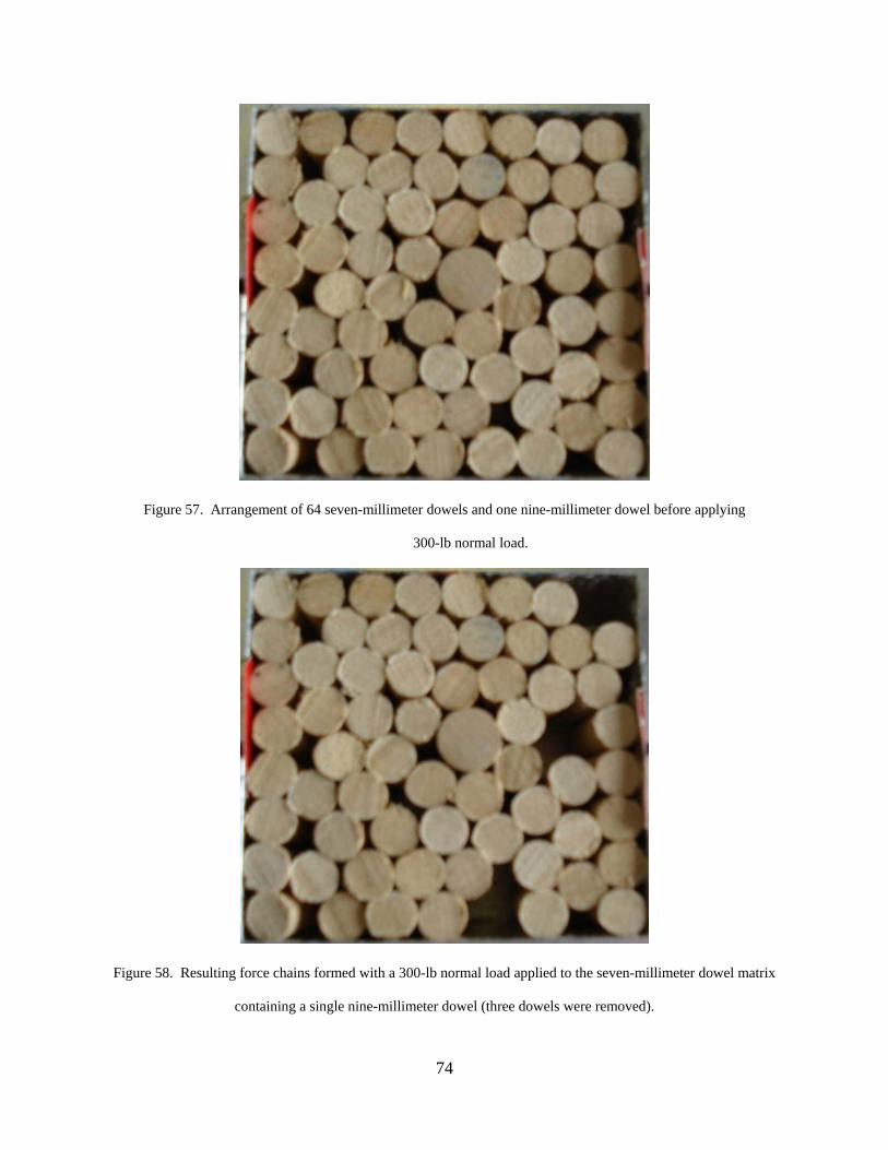
74

Figure 57. Arrangement of 64 seven-millimeter dowels and one nine-millimeter dowel before applying

300-lb normal load.

Figure 58. Resulting force chains formed with a 300-lb normal load applied to the seven-millimeter dowel matrix

containing a single nine-millimeter dowel (three dowels were removed).

75

The fractal fragmentation dimension of the dowel matrix was changed by inserting just

one dowel of a different size. It would not be practical to apply a power-law relationship to this

particular distribution, but logically, by increasing the size of one of the dowels, the size-

distribution of the dowels changes. Comparing the data between the first test of only identical

dowels and the second test employing the same dowels with one larger dowel included in the

mix, it appears that a change in the fractal fragmentation dimension of the matrix coincides with

a decrease in the formation of arches in the matrix.

The third test used a matrix of 60 seven-millimeter diameter dowels with 3 nine-

millimeter diameter dowels placed within the matrix (see Figure 58). Upon applying a 300-lb

normal load to the dowels, only two arches formed, as shown in Figure 60. Once again, by

varying the sizes of the dowels, fewer arches formed. Only three dowels were not engaged by

the force chains. Although the number of loose dowels did not vary from the previous test, the

number of arches formed did decrease. This indicates that more of the dowels are engaged in

actively transmitting the load to the dowels surrounding them than in the previous two tests.

Similar to adding one larger dowel, adding three larger dowels to the matrix also changes

the fractal fragmentation dimension of the matrix. Changing the size distribution of the dowels

to be less uniform and more “well-graded” again corresponds to a decrease in the number of

arches formed upon application of the 300-pound load.

76

Figure 59. Arrangement of 60 seven-millimeter dowels and 3 nine-millimeter dowel before applying

300-lb normal load.

Figure 60. Resulting force chains formed with a 300-lb normal load applied to the seven-millimeter dowel matrix

containing 3 nine-millimeter dowels (three dowels were removed).

77

The results of these tests using circular dowels confirm the hypothesis that the more well-

graded the distribution of dowels, the fewer arches are formed. The following tests will expand

this experiment to dowels of irregular shapes, a more realistic comparison to the Machu Picchu

walls.

The fourth test (Test A) used a mixture of 164 five-millimeter dowels that had been

chiseled to be asymmetrical and more closely resemble the seemingly random shapes of the

stones making up the walls at Machu Picchu. These dowels were packed into the direct shear

apparatus (Figure 61) in the same manner as the previous tests. A normal load of 400 lbs was

applied to the dowels, however, no arching developed, as shown in Figure 63. Upon reducing

the normal load applied to the dowels to 300 lbs, arches developed within the matrix of dowels,

as shown in Figure 64.

Figure 61. Test A –Arrangement of 164 five-millimeter irregular dowels before applying 400-lb normal load.

78

The dowels did not form arches when a 400-lb load was applied to them because each

dowel was engaged in transmitting a portion of the load. The larger load P applied to the dowels

generated more stress, σ, is applied as demonstrated in the following equation where A is the

area over which the force is applied:

(Equation 5.1)

If the dowels are in a square matrix with side length H, as the force is applied to the

matrix, it compresses an amount ΔH, as shown in Figure 61.

Figure 62. The dowel matrix compresses an amount ∆H when load is applied to it.

79

This compression causes strain in the dowels, expressed mathematically as

(Equation 5.2)

Stress and strain are related proportionally by Young’s Modulus, E.

(Equation 5.3)

So, the greater the load/stress applied to the dowels, the greater the strain developed by

the matrix. The greater strain indicates that a greater compression has occurred within the

dowels. One could imagine that this compression causes the dowels to deform such that greater

contact occurs between individual dowels, increasing the frictional resistance between individual

dowels and engaging all of the dowels in one large force chain, transmitting the load through

each dowel. The stones in the Machu Picchu walls are governed by this same law of mechanics,

however, Young’s Modulus for granite, estimated to be between 10.6 x 106 and 12.5 x 106 psi

(Lambe and Whitman, 1969), is far greater than that for wood, estimated to be about 8 x 105

(Mamlouk and Zaniewski, 1999), thus the compression experienced by stones under the same

conditions would be much less than that experienced by wood. This compression effect leads to

more contact between the individual units, strengthening the wall and helping it to act as one

monolithic unit rather than many small units.

80

Figure 63. Test A – Arrangement of 164 five-millimeter diameter irregular dowels after applying a 400-lb normal

load, before reducing the load to 300 lbs. Note that no arches developed when 400 lbs was applied.

Figure 64. Test A – Force chains developed after applying 300-lb normal load to the irregular five-millimeter

diameter dowels.

81

Figure 65 and Figure 66 show the fractal roughness and fragmentation plots, respectively.

The fractal fragmentation is multi-fractal, similar to the actual walls at Machu Picchu. The

fractal dimensions are summarized in Table 6.

Figure 65. Test A – P vs. A

Figure 66. Test A - a vs. N(A>a)

82

To decrease the fractal fragmentation dimension of the dowels and create a more well-

graded distribution, a single nine-millimeter dowel was placed into the five-millimeter dowel

matrix for Test B, shown in Figure 67. With a 300-lb normal load applied, one arch developed

as evidenced by Figure 68.

Figure 69 and Figure 70 show the plots used to determine the fractal roughness and

fragmentation dimensions of the dowel distribution in Test B, summarized in Table 4 and based

on a digitized image.

83

Figure 67. Test B – Arrangement of 159 five-millimeter irregular dowels with a single round nine-millimeter dowel

before applying 300-lb normal load.

Figure 68. Test B – After applying the 300-lb normal load to the dowel matrix, no force chains developed.

84

Figure 69. Test B – P vs. A

Figure 70. Test B - a vs. N(A>a)

For Test C, an additional 2 nine-millimeter dowels were added to the matrix (shown in

Figure 71) to further increase the fragmentation of the matrix. As shown in Figure 72, no force

chains developed.

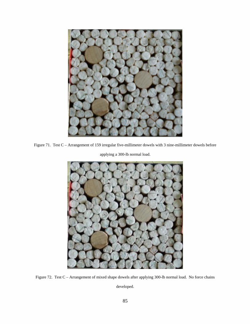
85

Figure 71. Test C – Arrangement of 159 irregular five-millimeter dowels with 3 nine-millimeter dowels before

applying a 300-lb normal load.

Figure 72. Test C – Arrangement of mixed shape dowels after applying 300-lb normal load. No force chains

developed.

86

Figure 73. Test C – P vs. A

Figure 74. Test C - a vs. N(A>a)

The plots used to determine the fractal roughness and fragmentation dimensions are

shown above and summarized in Table 6. The average fractal dimension once again decreased,

87

indicated that this distribution of dowels is even more controlled by the larger particles than

those in Tests A and B.

To even further increase the fractal fragmentation of the dowel size distribution, 3 nine-

millimeter and 5 seven-millimeter dowels were placed in a matrix of 153 five-millimeter

irregularly-shaped dowels for Test D, as demonstrated in Figure 75. As shown in Figure 76,

none of the dowels were loose and no arches formed upon applying the normal load. This

arrangement also engaged each individual dowel in transmitting the forces applied to the matrix.

The fractal fragmentation dimension shows that the distribution of dowels is once again even

more controlled by these larger elements than in the previous tests.

Figure 75. Arrangement of 153 irregular five-millimeter dowels with 3 nine-millimeter dowels and 5 seven-

millimeter dowels before applying a 300-lb normal load.

88

Figure 76. Arrangement of dowels after applying 300-lb normal load – no force chains developed.

Figure 77. Test D – P vs. A

89

Figure 78. Test C - a vs. N(A>a)

Table 6 indicates that with each successive test, the fractal roughness dimension, DR,

increased (indicating a greater variety of perimeter shapes) and the average fragmentation

dimension, DF, decreased as the slope of the line was influced by the larger dowels (indicating a

more well-graded mixture of dowel sizes). The fragmentation dimension of the dowel tests is

approaching the near-unity values of DF calculated for the retaining walls. This suggests that the

Incan walls are actually made up of a more well-graded distribution than even the dowels in Test

D, correlating with the lack of pop-out and toppling failures in the Incan walls.

The behavior summarized by these tests is significant for the Incan walls because their

composition is characterized by a wide range of stone sizes and roughness, similar to that of Test

D. While the identical dowels allowed more arches to develop, the varied dowels formed fewer

arches, because the varied sizes permitted more contact between the dowels and thus forces are

distributed in a more even fashion throughout the stones. The force of soil pushing against the

wall was simulated by pulling the dowels out with tweezers. If the retaining walls at Machu

90

Picchu weren’t engaging most of the stones making them up, the soil pushing against the wall

would force out the stones not engaged in the force chains, forming gaping arches where the soil

behind the walls could easily fall out from behind the wall. The lateral loads imposed by the

remaining soil behind the wall would be transferred to the remaining stones via the arching

effects of soil, causing widespread failures in the wall.

Table 6. Fractal Dimensions for laboratory Tests A, B, C, and D.

DR R2 DF R2 Arches Formed

Test A 0.786 0.906 13.3 0.649 8

Test B 0.896 0.951 9.16 0.673 1

Test C 0.923 0.972 6.78 0.662 0

Test D 0.927 0.984 5.90 0.785 0

The Inca engineers may have known this – building walls at Machu Picchu generally

exhibit much more uniform construction (as demonstrated in Section 4.2), while the retaining

walls are made up of varying sizes of stones. Perhaps this was an aesthetic choice; most likely

the walls are made up of varying sizes of stones because these retaining walls are of less

“importance”. Most of the complex, more aesthetically-pleasing stone work was likely reserved

for more important areas such as the royal residence or sacred sites.

91

5.4 STABILITY ANALYSIS REVISITED

As demonstrated, Machu Picchu’s retaining walls have a fractal size distribution as well as a

fractal roughness. As shown via the laboratory simulation with the direct shear apparatus, the

size distribution of the individual units is directly related to the amount of contact between the

units. When a set of uniform-sized dowels were tested, arches developed in the matrix, proving

that these dowels were not effectively transmitting loads through their contacts to their full

potential.

The stability analysis conducted in Section 3.0 assumed that friction was developed on

the entire surface area of the 1-ft by 2.5-ft block. However, the stability analysis also assumed

that the blocks were of a uniform size distribution. If the uniform-sized blocks in this analysis

behaved like the dowels studied in the laboratory simulation, these stones would not be fully

engaged in transmitting the load to one another and the contact between blocks would be

reduced. In the case of a popout failure, assuming that the bottom block of the wall was not

engaged with the stones above it, the normal force applied at the base of that block is only the

weight of the block itself, rather than the weight of the entire wall above it. It is also only

developing friction along its bottom, not the top. If this were the case, the popout factor of safety

would be reduced from 12.0 (as demonstrated in the initial stability analysis) to just 0.920, which

is not only up to our modern standards but is below unity, indicative of a failure.

This supports the hypothesis that the retaining walls at Machu Picchu garner at least some

of their inherent stability from the effects of fractals; the more effective packing of stones of

multiple sizes increases the effective transmission of loads through every particle in the wall,

engaging it in one monolithic structure.

92

6.0 CONCLUSION

The retaining walls at Machu Picchu are well-built and have endured with essentially no

maintenance since the city was abandoned centuries ago. The modular gravity granite block

walls were built on appropriately prepared foundations and exhibit adequate factors of safety

against sliding and overturning, generally comparable to those required by today’s engineers.

The walls have a fractal dimension in terms of roughness. The analysis carried out

indicates that the fractal roughness dimension varies from 0.94 to 1.16. The structural roughness

of the walls facilitates more contact between the individual wall elements, adding to the stability

of the wall. The distribution of elements in the wall is also fractal. This analysis shows that they

are actually multi-fractal over several ranges. This variety of sizes also encourages more contact

between the individual units making up the walls.

Via laboratory analogy with wooden dowels compressed in a direct shear apparatus, it is

confirmed that the fractal size distribution of the units making up the Machu Picchu walls

contributes to their stability; the more “well-graded” the matrix, the more contact forms between

the particles, thus each of the units is engaged in carrying the load applied to it.

Had the walls at Machu Picchu been constructed of identically-sized stones, fewer

contacts would exist between each of the stones in the walls. Fewer contacts between adjacent

stones would limit the transmission of loads between neighboring stones, effectively decreasing

the stability of the walls. The fractal distribution of units in the wall maximizes the packing of

93

stones within the wall while still allowing gaps between the stones to dissipate hydrostatic

pressure behind the wall.

In the future, this study may be improved by using other techniques (such as a different

digitizing system) to examine the fractal aspects of the walls. A more accurate stability analysis

could be conducted given more specific information about the conditions encountered in Machu

Picchu, should future excavations or test borings be permitted at the site to glean the appropriate

engineering properties of the soil. Given well-publicized recent tectonic activity in western

South America, a more detailed seismic study could be conducted to gather information about

the Incan engineers’ knowledge of seismic design.

Today’s modular retaining walls may be improved by considering a fractal distribution of

units throughout the wall. Precast concrete units of various sizes with substantial roughness

could easily be mass-produced and sold as a package for retaining wall construction. Rather than

manufacturing 900 units of “Size X,” manufacturers could produce 300 units of “Size X,” 300

units of “Size Y,” and 300 units of “Size Z.” Combining the concept of fractals with modern

modular wall design could lead to longer-lasting, more stable retaining walls.

Perhaps the Incan engineers, through their experiences in other areas of their empire,

observed these principals at work (through trial and error) and intentionally constructed the walls

with a fractal distribution and adequate factors of safety. Perhaps it was an aesthetic choice.

Perhaps the choice was driven by economics. If the Incan engineers thought the way modern

engineers think, it was a combination of all of these factors. Regardless of the motivation, the

Incan engineers knew how to construct lasting infrastructure. The Incan infrastructure withstood

centuries of neglect and remains intact; much of our modern infrastructure receives some

94

maintenance (though frequently not nearly as much as it should) and still fails much sooner than

that of the Incan empire.

The concept of fractals can be applied to the retaining walls of Machu Picchu and several

aspects of geotechnical engineering, including crushing of granular materials and grain-size

distribution analysis. Perhaps fractal theory will make its way into other civil engineering

disciplines. Someday engineers may find ways to employ them in the design and analysis of

bridges, structures, pavements, or water systems.

95

APPENDIX A

TABULATION OF WALL UNIT AREAS AND PERIMETERS

A.1 WALL 1

Stone

Area

(m2)Perim.

(m) N(A>a) Stone

Area

(m2)Perim.

(m) N(A>a)147 0.667 3.65 0 214 0.0587 0.988 2314 0.325 2.49 1 249 0.0575 1.02 2433 0.214 1.86 2 181 0.0560 0.945 2573 0.212 1.92 3 6 0.0552 0.949 26

120 0.171 1.81 4 99 0.0534 0.937 27137 0.161 1.92 5 252 0.0530 1.103 28203 0.125 1.51 6 76 0.0518 0.940 29172 0.104 1.29 7 133 0.0512 0.850 30153 0.0857 1.24 8 93 0.0512 0.918 3154 0.0779 1.05 9 34 0.0508 0.894 3250 0.0766 1.12 10 11 0.0497 0.856 3388 0.0766 1.04 11 139 0.0490 0.856 34

105 0.0751 1.12 12 127 0.0485 0.883 35138 0.0701 1.16 13 5 0.0472 0.829 36215 0.0699 1.05 14 173 0.0471 0.899 37

8 0.0697 1.02 15 213 0.0458 0.814 3830 0.0661 1.07 16 16 0.0454 0.845 3985 0.0658 0.972 17 45 0.0450 0.891 40

200 0.0655 1.02 18 107 0.0450 0.866 41205 0.0638 1.09 19 245 0.0447 0.848 42194 0.0631 0.969 20 224 0.0445 0.849 4366 0.0619 0.994 21 117 0.0433 0.813 4436 0.0606 1.04 22 37 0.0431 0.810 45

96

Stone

Area

(m2)Perim.

(m) N(A>a) Stone

Area

(m2)Perim.

(m) N(A>a)81 0.0426 0.821 46 115 0.0323 0.742 8653 0.0425 0.800 47 149 0.0323 0.788 8757 0.0425 1.04 48 170 0.0322 0.755 88

175 0.0419 0.845 49 157 0.0320 0.767 8938 0.0417 0.827 50 219 0.0313 0.746 90

240 0.0414 0.837 51 158 0.0312 0.745 91196 0.0411 0.811 52 15 0.0311 0.766 92142 0.0408 0.794 53 111 0.0303 0.790 93199 0.0408 0.863 54 185 0.0301 0.731 94146 0.0406 0.774 55 223 0.0295 0.689 95174 0.0404 0.794 56 238 0.0288 0.662 96218 0.0403 0.759 57 243 0.0281 0.725 97145 0.0400 0.777 58 109 0.0280 0.730 98230 0.0397 0.842 59 126 0.0280 0.673 99

2 0.0396 0.961 60 48 0.0278 0.820 100124 0.0395 0.791 61 154 0.0274 0.743 101129 0.0395 0.757 62 220 0.0272 0.699 102166 0.0388 0.787 63 204 0.0264 0.614 103162 0.0388 0.824 64 246 0.0261 0.755 104242 0.0385 0.907 65 1 0.0261 0.599 10577 0.0378 0.877 66 104 0.0260 0.668 10696 0.0378 0.796 67 144 0.0258 0.637 107

141 0.0371 0.750 68 29 0.0248 0.635 108189 0.0370 0.776 69 4 0.0246 0.677 10970 0.0369 0.796 70 21 0.0244 0.685 110

177 0.0368 0.785 71 171 0.0241 0.644 111110 0.0367 0.958 72 40 0.0240 0.660 112225 0.0366 0.766 73 113 0.0237 0.610 11318 0.0359 0.822 74 31 0.0228 0.581 11425 0.0358 0.753 75 55 0.0224 0.695 115

187 0.0356 0.764 76 253 0.0224 0.633 116206 0.0353 0.752 77 67 0.0218 0.552 11784 0.0348 0.806 78 39 0.0211 0.588 11878 0.0345 0.727 79 27 0.0210 0.624 11922 0.0333 0.787 80 161 0.0210 0.608 120

202 0.0327 0.820 81 7 0.0209 0.545 121250 0.0325 0.730 82 184 0.0195 0.594 12282 0.0325 0.712 83 193 0.0194 0.572 123

134 0.0324 0.821 84 9 0.0193 0.521 124234 0.0323 0.673 85 227 0.0187 0.520 125

97

Stone Area (m2)Perim.

(m) N(A>a) Stone Area (m2)Perim.

(m) N(A>a)216 0.0185 0.540 126 10 0.00553 0.364 16623 0.0182 0.520 127 140 0.00553 0.299 167

119 0.0172 0.515 128 28 0.00540 0.365 16812 0.0156 0.690 129 150 0.00521 0.408 169

192 0.0145 0.513 130 229 0.00512 0.291 170176 0.0139 0.533 131 231 0.00511 0.308 171163 0.0129 0.460 132 211 0.00507 0.310 172217 0.0128 0.487 133 71 0.00506 0.267 17360 0.0124 0.415 134 35 0.00504 0.331 174

244 0.0121 0.432 135 68 0.00491 0.293 175237 0.0120 0.459 136 86 0.00490 0.291 176239 0.0115 0.607 137 95 0.00460 0.282 177221 0.0110 0.430 138 20 0.00458 0.284 178241 0.0108 0.494 139 97 0.00455 0.277 179148 0.0107 0.398 140 108 0.00434 0.386 180156 0.0104 0.566 141 59 0.00433 0.254 181112 0.0100 0.396 142 114 0.00428 0.273 182251 0.00954 0.471 143 136 0.00407 0.259 183165 0.00917 0.395 144 69 0.00387 0.247 184198 0.00890 0.365 145 87 0.00385 0.251 185235 0.00864 0.528 146 152 0.00373 0.295 18619 0.00861 0.386 147 106 0.00372 0.267 187

210 0.00832 0.400 148 254 0.00354 0.218 188100 0.00816 0.388 149 3 0.00351 0.304 18917 0.00782 0.425 150 42 0.00340 0.242 190

121 0.00746 0.340 151 228 0.00332 0.243 19183 0.00740 0.398 152 201 0.00321 0.250 192

151 0.00738 0.354 153 74 0.00312 0.239 19375 0.00736 0.327 154 232 0.00309 0.230 19449 0.00732 0.463 155 98 0.00301 0.214 195

197 0.00727 0.401 156 63 0.00300 0.259 196116 0.00706 0.335 157 135 0.00296 0.248 197236 0.00700 0.329 158 186 0.00283 0.212 198123 0.00698 0.367 159 143 0.00281 0.211 19962 0.00666 0.327 160 159 0.00271 0.217 200

122 0.00659 0.386 161 233 0.00269 0.222 20172 0.00637 0.335 162 195 0.00268 0.206 202

180 0.00611 0.357 163 190 0.00264 0.201 20390 0.00581 0.388 164 13 0.00260 0.205 20451 0.00580 0.381 165 94 0.00256 0.203 205

98

Stone Area (m2)Perim.

(m) N(A>a) Stone Area (m2)Perim.

(m) N(A>a)160 0.00250 0.207 206 80 0.00151 0.161 22058 0.00245 0.290 207 79 0.00149 0.151 221

226 0.00237 0.200 208 128 0.00141 0.161 22256 0.00233 0.226 209 247 0.00139 0.198 223

248 0.00227 0.220 210 26 0.00133 0.161 224179 0.00211 0.201 211 91 0.00125 0.186 225155 0.00190 0.199 212 188 0.00119 0.165 226183 0.00187 0.185 213 178 0.000901 0.122 227125 0.00182 0.171 214 212 0.000855 0.178 228191 0.00179 0.157 215 32 0.000845 0.111 229118 0.00177 0.163 216 24 0.000827 0.119 23061 0.00171 0.210 217 164 0.000604 0.112 23146 0.00167 0.167 218 92 0.000381 0.0998 232

222 0.00158 0.168 219 89 0.000316 0.0736 233

A.2 WALL 2

Stone Area (m2)Perim.

(m) N(A>a) Stone Area (m2)Perim.

(m) N(A>a)74 0.620 3.06 0 7 0.0466 0.897 1613 0.608 3.11 1 99 0.0402 0.803 1741 0.350 2.29 2 12 0.0397 0.792 1888 0.227 1.92 3 96 0.0370 0.776 1917 0.135 1.46 4 32 0.0366 0.821 2062 0.111 1.32 5 47 0.0356 0.828 2118 0.111 1.47 6 69 0.0335 0.795 22

101 0.0893 1.45 7 53 0.0299 0.669 2314 0.0892 1.28 8 39 0.0254 0.682 249 0.0764 1.16 9 72 0.0235 0.645 25

28 0.0689 1.04 10 26 0.0230 0.596 2681 0.0623 1.09 11 75 0.0226 0.674 2780 0.0594 0.967 12 30 0.0193 0.526 288 0.0554 1.09 13 57 0.0175 0.599 29

63 0.0530 0.898 14 6 0.0161 0.517 3044 0.0482 0.839 15 61 0.0150 0.574 31

99

Stone Area (m2)Perim.

(m) N(A>a) Stone Area (m2)Perim.

(m) N(A>a)36 0.0138 0.502 32 89 0.00407 0.304 584 0.0133 0.430 33 102 0.00387 0.262 59

48 0.0121 0.505 34 90 0.00386 0.232 6085 0.0114 0.554 35 19 0.00372 0.243 6156 0.0114 0.512 36 103 0.00353 0.272 6235 0.0102 0.451 37 42 0.00327 0.268 6383 0.0100 0.442 38 27 0.00317 0.221 6493 0.00952 0.409 39 79 0.00308 0.226 6538 0.00896 0.456 40 3 0.00306 0.238 665 0.00847 0.386 41 16 0.00306 0.233 67

25 0.00807 0.388 42 29 0.00282 0.220 6887 0.00707 0.412 43 49 0.00264 0.240 6915 0.00699 0.352 44 20 0.00221 0.229 7076 0.00699 0.339 45 84 0.00154 0.200 71

100 0.00697 0.343 46 24 0.00120 0.136 7246 0.00661 0.334 47 54 0.00108 0.139 7343 0.00638 0.332 48 86 0.000715 0.103 7434 0.00624 0.332 49 60 0.000492 0.0937 7550 0.00544 0.353 50 37 0.000465 0.0929 7645 0.00519 0.391 51 78 0.000455 0.0873 7755 0.00475 0.285 52 73 0.000418 0.118 7840 0.00465 0.389 53 82 0.000418 0.0896 7933 0.00449 0.275 54 77 0.000269 0.0968 8094 0.00445 0.312 55 52 0.000223 0.0645 8111 0.00439 0.371 56 106 0.000204 0.0703 8270 0.00416 0.313 57 51 0.000195 0.0638 83

100

A.3 WALL 3

Stone Area (m2)Perim.

(m) N(A>a) Stone Area (m2)Perim.

(m) N(A>a)53 0.404 2.83 0 42 0.0341 0.789 3312 0.127 1.44 1 95 0.0337 0.772 3425 0.0963 1.22 2 21 0.0332 0.748 3515 0.0841 1.25 3 114 0.0328 0.823 3672 0.0813 1.12 4 77 0.0327 0.801 37

111 0.0812 1.11 5 88 0.0318 0.703 3850 0.0807 1.08 6 86 0.0281 0.635 3980 0.0715 1.07 7 30 0.0267 0.666 4074 0.0701 1.06 8 112 0.0267 0.677 4143 0.0670 1.05 9 75 0.0258 0.693 4251 0.0662 1.06 10 135 0.0245 0.606 4357 0.0644 1.05 11 85 0.0242 0.665 4491 0.0639 0.988 12 55 0.0237 0.673 4570 0.0634 1.11 13 106 0.0231 0.644 4610 0.0615 1.17 14 120 0.0230 0.613 472 0.0611 1.22 15 113 0.0229 0.651 48

131 0.0605 0.989 16 26 0.0225 0.550 4948 0.0594 1.01 17 6 0.0213 0.707 5081 0.0498 0.892 18 11 0.0209 0.573 5117 0.0493 0.846 19 92 0.0201 0.634 5237 0.0493 0.900 20 93 0.0197 0.587 53

104 0.0470 0.851 21 121 0.0178 0.516 5447 0.0436 0.831 22 8 0.0172 0.691 55

101 0.0426 0.941 23 23 0.0165 0.578 56119 0.0412 0.813 24 137 0.0163 0.540 5797 0.0408 0.795 25 5 0.0162 0.630 5879 0.0391 0.822 26 4 0.0152 0.550 5978 0.0385 0.847 27 7 0.0149 0.536 60

125 0.0367 0.737 28 49 0.0147 0.473 619 0.0360 0.848 29 54 0.0127 0.598 62

82 0.0359 0.799 30 59 0.0106 0.419 6329 0.0348 0.776 31 44 0.0101 0.417 64

130 0.0348 0.723 32 96 0.00988 0.429 65

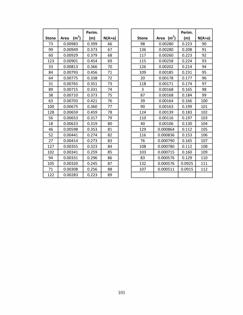
101

Stone Area (m2)Perim.

(m) N(A>a) Stone Area (m2)Perim.

(m) N(A>a)73 0.00983 0.399 66 98 0.00280 0.223 9099 0.00949 0.373 67 136 0.00280 0.208 9160 0.00929 0.379 68 117 0.00260 0.223 92

123 0.00901 0.454 69 115 0.00258 0.224 9333 0.00813 0.366 70 126 0.00202 0.214 9484 0.00793 0.456 71 109 0.00185 0.231 9564 0.00775 0.338 72 20 0.00178 0.177 9631 0.00765 0.351 73 118 0.00171 0.174 9789 0.00715 0.331 74 3 0.00168 0.165 9838 0.00710 0.373 75 87 0.00168 0.184 9963 0.00703 0.421 76 39 0.00164 0.166 100

100 0.00675 0.360 77 90 0.00163 0.199 101128 0.00659 0.459 78 124 0.00139 0.183 10256 0.00653 0.317 79 110 0.00116 0.197 10318 0.00623 0.319 80 40 0.00106 0.130 10446 0.00598 0.353 81 129 0.000864 0.112 10552 0.00441 0.274 82 116 0.000836 0.153 10627 0.00414 0.273 83 76 0.000790 0.165 107

127 0.00355 0.323 84 108 0.000780 0.112 108102 0.00341 0.259 85 103 0.000715 0.160 10994 0.00331 0.296 86 83 0.000576 0.129 110

105 0.00320 0.245 87 132 0.000576 0.0925 11171 0.00308 0.256 88 107 0.000511 0.0915 112

122 0.00283 0.223 89

102

A.4 WALL 4

Stone Area (m2)Perim.

(m) N(A>a) Stone Area (m2)Perim.

(m) N(A>a)61 0.345 2.31 0 270 0.0381 0.779 3355 0.284 2.22 1 100 0.0364 0.766 34

126 0.183 1.89 2 258 0.0352 0.707 3533 0.176 1.76 3 183 0.0352 0.772 36

165 0.147 1.78 4 123 0.0346 0.794 37158 0.0789 1.08 5 34 0.0346 0.707 3864 0.0762 1.14 6 286 0.0345 0.748 39

215 0.0760 1.13 7 58 0.0337 0.756 40114 0.0661 1.16 8 73 0.0332 0.763 4111 0.0640 1.09 9 266 0.0300 0.682 4272 0.0629 0.312 10 238 0.0298 0.721 43

106 0.0619 1.02 11 190 0.0289 0.700 4422 0.0587 1.03 12 138 0.0286 0.819 45

274 0.0579 1.09 13 208 0.0270 0.617 46116 0.0549 1.07 14 66 0.0252 0.686 47289 0.0546 0.913 15 299 0.0242 0.648 48295 0.0539 0.949 16 221 0.0240 0.611 49121 0.0519 0.889 17 281 0.0227 0.642 50110 0.0508 0.899 18 10 0.0214 0.594 51237 0.0506 0.942 19 230 0.0213 0.610 52197 0.0504 0.914 20 234 0.0212 0.631 53137 0.0473 0.878 21 5 0.0206 0.715 54177 0.0464 0.897 22 153 0.0205 0.628 55171 0.0441 0.857 23 235 0.0203 0.534 56224 0.0436 0.900 24 213 0.0195 0.598 5791 0.0417 0.797 25 31 0.0192 0.568 5870 0.0416 0.861 26 273 0.0191 0.533 5982 0.0399 0.808 27 252 0.0191 0.564 60

218 0.0397 0.861 28 19 0.0190 0.549 61283 0.0394 0.790 29 189 0.0174 0.502 62140 0.0388 0.820 30 86 0.0165 0.546 6377 0.0386 0.861 31 20 0.0164 0.486 64

297 0.0382 0.894 32 29 0.0161 0.526 65

103

Stone Area (m2)Perim.

(m) N(A>a) Stone Area (m2)Perim.

(m) N(A>a)79 0.0153 0.641 66 134 0.00781 0.373 10663 0.0152 0.592 67 62 0.00780 0.404 107

260 0.0145 0.461 68 139 0.00735 0.381 108161 0.0144 0.491 69 129 0.00717 0.358 10921 0.0141 0.477 70 103 0.00709 0.395 110

119 0.0141 0.519 71 261 0.00709 0.352 111199 0.0139 0.525 72 52 0.00687 0.343 11278 0.0138 0.453 73 150 0.00653 0.305 1136 0.0135 0.490 74 135 0.00652 0.343 114

50 0.0128 0.434 75 166 0.00641 0.401 115173 0.0121 0.436 76 107 0.00637 0.321 116223 0.0119 0.445 77 54 0.00631 0.331 117298 0.0119 0.464 78 267 0.00630 0.347 11849 0.0118 0.453 79 132 0.00623 0.302 11912 0.0112 0.424 80 105 0.00609 0.347 12081 0.0112 0.424 81 255 0.00604 0.310 121

259 0.0110 0.400 82 216 0.00565 0.387 122156 0.0109 0.422 83 226 0.00561 0.313 12384 0.0107 0.432 84 239 0.00558 0.286 12483 0.0104 0.483 85 89 0.00556 0.281 125

180 0.0101 0.406 86 95 0.00555 0.328 126112 0.0101 0.393 87 104 0.00552 0.302 127194 0.00983 0.418 88 144 0.00540 0.300 128145 0.00960 0.381 89 69 0.00534 0.318 12946 0.00943 0.386 90 174 0.00529 0.299 130

210 0.00943 0.372 91 172 0.00516 0.323 131225 0.00937 0.368 92 67 0.00506 0.267 13287 0.00886 0.389 93 219 0.00504 0.283 133

206 0.00874 0.038 94 28 0.00481 0.301 13459 0.00869 0.373 95 212 0.00472 0.275 13575 0.00867 0.350 96 133 0.00471 0.326 13671 0.00854 0.418 97 99 0.00468 0.298 137

157 0.00849 0.422 98 131 0.00455 0.287 138164 0.00844 0.391 99 127 0.00443 0.353 13951 0.00838 0.372 100 290 0.00440 0.285 140

229 0.00836 0.363 101 9 0.00437 0.257 141214 0.00820 0.373 102 25 0.00436 0.263 14256 0.00818 0.377 103 244 0.00434 0.251 14376 0.00817 0.381 104 186 0.00431 0.263 144

179 0.00799 0.400 105 202 0.00428 0.311 145

104

Stone Area (m2)Perim.

(m) N(A>a) Stone Area (m2)Perim.

(m) N(A>a)27 0.00425 0.294 146 175 0.00255 0.243 186

302 0.00425 0.262 147 265 0.00255 0.206 187204 0.00419 0.275 148 113 0.00246 0.219 188109 0.00418 0.263 149 228 0.00242 0.210 189122 0.00418 0.315 150 48 0.00239 0.212 190170 0.00413 0.324 151 263 0.00239 0.233 191195 0.00410 0.250 152 88 0.00226 0.208 19215 0.00404 0.275 153 120 0.00226 0.228 193

130 0.00401 0.294 154 304 0.00219 0.187 194143 0.00395 0.360 155 37 0.00218 0.201 195253 0.00389 0.282 156 196 0.00214 0.194 19665 0.00387 0.245 157 117 0.00211 0.208 197

152 0.00386 0.245 158 287 0.00211 0.191 198162 0.00380 0.254 159 198 0.00206 0.205 199149 0.00373 0.251 160 176 0.00191 0.206 20092 0.00369 0.233 161 232 0.00187 0.177 201

142 0.00369 0.251 162 169 0.00186 0.165 20260 0.00367 0.244 163 182 0.00184 0.185 203

128 0.00358 0.260 164 90 0.00178 0.203 20430 0.00352 0.246 165 146 0.00173 0.217 205

160 0.00348 0.242 166 168 0.00171 0.223 206181 0.00347 0.243 167 167 0.00169 0.194 207155 0.00345 0.242 168 200 0.00164 0.161 208111 0.00342 0.246 169 18 0.00162 0.183 209280 0.00333 0.238 170 271 0.00156 0.159 210251 0.00331 0.286 171 124 0.00155 0.162 211231 0.00330 0.242 172 192 0.00151 0.162 212285 0.00315 0.234 173 96 0.00148 0.209 213222 0.00313 0.230 174 118 0.00142 0.176 214191 0.00311 0.240 175 249 0.00135 0.161 215294 0.00308 0.314 176 141 0.00134 0.231 216233 0.00290 0.212 177 292 0.00132 0.166 217282 0.00288 0.207 178 74 0.00131 0.154 218296 0.00286 0.266 179 108 0.00124 0.150 219115 0.00278 0.231 180 220 0.00122 0.165 220178 0.00278 0.258 181 57 0.00119 0.149 22139 0.00272 0.258 182 264 0.00116 0.131 222

243 0.00266 0.200 183 184 0.00113 0.172 22397 0.00260 0.229 184 205 0.00113 0.135 224

188 0.00258 0.266 185 209 0.00113 0.143 225

105

Stone Area (m2)Perim.

(m) N(A>a) Stone Area (m2)Perim.

(m) N(A>a)201 0.00111 0.135 226 193 0.000567 0.122 242217 0.00111 0.133 227 279 0.000539 0.110 243293 0.00109 0.154 228 203 0.000474 0.0881 24417 0.00108 0.143 229 125 0.000465 0.0874 24598 0.00108 0.141 230 163 0.000455 0.108 2467 0.000975 0.150 231 3 0.000437 0.0778 247

236 0.000966 0.124 232 47 0.000437 0.112 248275 0.000883 0.137 233 68 0.000409 0.0799 24993 0.000845 0.129 234 38 0.000316 0.0988 250

227 0.000845 0.119 235 262 0.000269 0.0780 251187 0.000780 0.109 236 185 0.000223 0.0650 252207 0.000771 0.108 237 102 0.000204 0.0541 25394 0.000753 0.111 238 53 0.000158 0.0598 254

136 0.000697 0.100 239 278 0.000139 0.0484 255148 0.000687 0.102 240 301 9.29E-05 0.0357 256159 0.000632 0.101 241 101 4.65E-05 0.0243 257

A.5 WALL 5

Stone Area (m2)Perim.

(m) N(A>a) Stone Area (m2)Perim.

(m) N(A>a)199 0.146 1.75 0 78 0.0887 1.21 1675 0.145 1.68 1 226 0.0875 1.15 17

208 0.142 1.53 2 196 0.0853 1.28 18136 0.133 1.57 3 212 0.0847 1.37 1919 0.121 1.61 4 215 0.0805 1.19 20

132 0.110 1.50 5 85 0.0789 1.18 21192 0.106 1.29 6 134 0.0773 1.27 22195 0.106 1.25 7 91 0.0770 1.11 23185 0.105 1.32 8 96 0.0762 1.21 24193 0.104 1.42 9 142 0.0749 1.15 25228 0.0999 1.40 10 83 0.0735 1.23 2632 0.0936 1.27 11 86 0.0735 1.12 27

220 0.0928 1.26 12 227 0.0733 1.14 2826 0.0924 1.45 13 92 0.0708 1.09 29

135 0.0917 1.24 14 38 0.0696 1.30 3097 0.0901 1.25 15 29 0.0691 1.27 31

106

Stone Area (m2)Perim.

(m) N(A>a) Stone Area (m2)Perim.

(m) N(A>a)191 0.0687 1.02 32 79 0.0296 0.676 65205 0.0687 1.03 33 217 0.0296 0.673 6636 0.0684 1.17 34 144 0.0276 0.629 67

197 0.0634 1.01 35 137 0.0270 0.764 6893 0.0623 1.08 36 203 0.0248 0.792 69

131 0.0620 1.07 37 94 0.0235 0.589 7017 0.0620 1.15 38 28 0.0232 0.577 7189 0.0615 0.944 39 88 0.0215 0.568 72

190 0.0613 1.00 40 225 0.0208 0.554 73143 0.0601 1.24 41 209 0.0199 0.537 74211 0.0580 1.26 42 22 0.0191 0.732 7520 0.0578 1.06 43 25 0.0187 0.511 7687 0.0572 1.19 44 18 0.0170 0.596 7716 0.0556 0.909 45 23 0.0167 0.538 78

224 0.0538 0.973 46 213 0.0130 0.478 79139 0.0523 1.03 47 84 0.0106 0.481 8015 0.0497 0.876 48 207 0.00937 0.383 8180 0.0484 0.837 49 218 0.00805 0.617 8221 0.0471 0.903 50 216 0.00728 0.412 83

221 0.0469 0.850 51 27 0.00699 0.534 8490 0.0456 0.829 52 194 0.00685 0.336 8533 0.0454 0.896 53 198 0.00450 0.319 8677 0.0444 0.916 54 81 0.00372 0.268 87

222 0.0444 1.09 55 219 0.00360 0.263 8831 0.0430 1.04 56 133 0.00352 0.277 89

214 0.0419 0.793 57 140 0.00349 0.297 9095 0.0417 0.850 58 204 0.00339 0.360 9124 0.0386 0.771 59 200 0.00293 0.498 92

210 0.0359 0.915 60 201 0.00261 0.271 93138 0.0339 0.975 61 206 0.00193 0.164 94202 0.0326 0.802 62 223 0.00159 0.172 9582 0.0324 0.758 63 141 0.00118 0.159 9634 0.0302 0.675 64

107

BIBLIOGRAPHY

ABC-CLIO. (2001). Encyclopedia of Archaeology: History and Discoveries. Retrieved April 2009, from Inca: http://www.credoreference.com/engry/8056707.

ABC-CLIO. (2001). Encyclopedia of Archaeology: History and Discoveries. Retrieved April 2009, from Machu Picchu: http://www.credoreference.com/engry/8056789.

AUTOCAD LT. Autodesk, Inc., 2007.

Boast, C.W. and Baveye, P., “Fractal Geometry, Fragmentation Processes and the Physics of Scale-Invariance: An Introduction.” Fractals in the Earth Sciences. Philippe Baveye, Jean-Yves Parlange, and Bobby A. Steward (eds.). Florida: CRC Press, 1998, pp. 1-54.

Bray, J.W. and Hoek, E. Rock Slope Engineering. London: The Institute of Mining and

Metallurgy, 1981. Das, Braja M. Principals of Foundation Engineering. 5th ed. Pacific Grove: Brooks/Cole – Thompson, 2004. Gabor, Korvin. Fractal Models in the Earth Sciences. Amsterdam: Elsevier Science Publishers, 1992. Lambe, T. William and Robert V. Whitman. Soil Mechanics. New York: John Wiley and Sons,

1969. Mandelbrot, Benoit B. Fractals: Form, Chance, ad Dimension. San Francisco: W.H. Freeman and Company, 1977. Mandelbrot, Benoit B. The Fractal Geometry of Nature. San Francisco: W.H. Freeman and

Company, 1982. Russ, John C. Fractal Surfaces. New York: Plenum Press, 1994. Vilimek, V., J. Kimes, J. Vlcko, and R. Carreno. “Catastrophic Debris Flows Near Machu Picchu Village (Aguas Calientes), Peru.” Environmental Geology. 2006, pp. 1041-1052.

108

Vallejo, L.E., Sebastian Lobo-Guerrero, and Zamri Chik. “A Network of Fractal Force Chains and Their Effect in Granular Materials Under Compression.” Fractals in Engineering. Jacques Levy-Vehel and Evelyne Lutton. Springer, 2005, pp. 67-80. Vallejo, L.E. and James P. Hyslip. “Fractal Analysis of the Roughness and Size Distribution of Granular Materials.” Engineering Geology. 1997, pp. 231-244. Vallejo, L.E. “A Plane Stress Direct Shear Apparatus for Testing Clays” In: Geotechnical

Engineering Congress 1991. F.G. McLean, D.A. Campbell, and D.W. Harris (eds.), Geotechnical Special Publication 27, Vol. II. American Society of Civil Engineers, pp. 851-862.

Von Daniken, Erich. Chariots of the Gods. New York: Bantam Books, 1971. Wright, Kenneth R. and Alfredo Valencia Zegarra. Machu Picchu: A Civil Engineering Marvel. Reston, Virginia: ASCE Press, 2000. Yoshida, Yojiro. “Force Chains and the Fragmentation of Granular Materials.” Master’s Thesis.

Department of Civil and Environmental Engineering, University of Pittsburgh, 2004. Zaniewski, John P. and Michael S. Mamlouk. Materials for Civil and Construction Engineers. Menlo Park: Addison Wesley Longman, Inc., 1999.