Embed Size (px)
Citation preview
A Specialised Constraint Approach for
Stable Matching Problems
by
Chris Unsworth
A thesis submitted in fulfilment of the requirements
for the Degree of Doctor of Philosophy
Department of Computing Science
Information and Mathematical Sciences.
University of Glasgow
2008

i
Abstract
Constraint programming is a generalised framework designed to solve combinatorial prob-
lems. This framework is made up of a set of predefined independent components and
generalised algorithms. This is a very versatile structure which allows for a variety of rich
combinatorial problems to be represented and solved relatively easily.
Stable matching problems consist of a set of participants wishing to be matched into
pairs or groups in a stable manner. A matching is said to be stable if there is no pair
or group of participants that would rather make a private arrangement to improve their
situation and thus undermine the matching. There are many important “real life” ap-
plications of stable matching problems across the world. Some of which includes the
Hospitals/Residents problem in which a set of graduating medical students, also known
as residents, need to be assigned to hospital posts. Some authorities assign children to
schools as a stable matching problem. Many other such problems are also tackled as sta-
ble matching problems. A number of classical stable matching problems have efficient
specialised algorithmic solutions.
Constraint programming solutions to stable matching problems have been investigated
in the past. These solutions have been able to match the theoretically optimal time
complexities of the algorithmic solutions. However, empirical evidence has shown that in
reality these constraint solutions run significantly slower than the specialised algorithmic
solutions. Furthermore, their memory requirements prohibit them from solving problems
which the specialised algorithmic solutions can solve in a fraction of a second.
My contribution investigates the possibility of modelling stable matching problems as
specialised constraints. The motivation behind this approach was to find solutions to these
problems which maintain the versatility of the constraint solutions, whilst significantly
reducing the performance gap between constraint and specialised algorithmic solutions.
To this end specialised constraint solutions have been developed for the stable marriage
problem and the Hospitals/Residents problem. Empirical evidence has been presented
which shows that these solutions can solve significantly larger problems than previously
published constraint solutions. For these larger problem instances it was seen that the
specialised constraint solutions came within a factor of four of the time required by al-
gorithmic solutions. It has also been shown that, through further specialisation, these
constraint solutions can be made to run significantly faster. However, these improvements
came at the cost of versatility. As a demonstration of the versatility of these solutions

ii
it is shown that, by adding simple side constraints, richer problems can be easily mod-
elled. These richer problems add additional criteria and/or an optimisation requirement
to the original stable matching problems. Many of these problems have been proven to be
NP-Hard and some have no known algorithmic solutions. Included with these models are
results from empirical studies which show that these are indeed feasible solutions to the
richer problems. Results from the studies also provide some insight into the structure of
these problems, some of which have had little or no previous study.
Contents
1 Introduction 1
2 Literature review 3
2.1 The constraint satisfaction problem . . . . . . . . . . . . . . . . . . . . . . . 3
2.1.1 Node-consistency . . . . . . . . . . . . . . . . . . . . . . . . . . . . . 6
2.1.2 Arc-consistency . . . . . . . . . . . . . . . . . . . . . . . . . . . . . . 6
2.1.3 Generalised arc-consistency . . . . . . . . . . . . . . . . . . . . . . . 7
2.1.4 Path consistency . . . . . . . . . . . . . . . . . . . . . . . . . . . . . 8
2.1.5 Singleton consistency . . . . . . . . . . . . . . . . . . . . . . . . . . . 8
2.2 Literature review of arc-consistency . . . . . . . . . . . . . . . . . . . . . . . 8
2.2.1 Introduction . . . . . . . . . . . . . . . . . . . . . . . . . . . . . . . 8
2.2.2 Coarse grained arc-consistency algorithms . . . . . . . . . . . . . . . 8
2.2.3 Fine grained arc-consistency algorithms . . . . . . . . . . . . . . . . 11
2.2.4 Generic algorithms . . . . . . . . . . . . . . . . . . . . . . . . . . . . 13
2.2.5 Constraint solvers . . . . . . . . . . . . . . . . . . . . . . . . . . . . 17
2.2.6 Global constraints . . . . . . . . . . . . . . . . . . . . . . . . . . . . 18
2.3 Stable matching problems . . . . . . . . . . . . . . . . . . . . . . . . . . . . 19
2.3.1 The Stable Marriage problem . . . . . . . . . . . . . . . . . . . . . . 19
2.3.2 Incomplete preference lists . . . . . . . . . . . . . . . . . . . . . . . . 21
2.3.3 Ties in preference lists . . . . . . . . . . . . . . . . . . . . . . . . . . 22
2.3.4 Ties and incomplete preference lists . . . . . . . . . . . . . . . . . . 23
2.3.5 Hospitals/Residents problem . . . . . . . . . . . . . . . . . . . . . . 24
2.3.6 Stable Roommates problem . . . . . . . . . . . . . . . . . . . . . . . 27
2.4 Constraint programming approaches to stable matching problems . . . . . . 30
2.4.1 Constraint models for stable matching problems . . . . . . . . . . . 31
iii
CONTENTS iv
2.4.2 Evaluating the constraint stable marriage solutions . . . . . . . . . . 42
2.4.3 Conclusion . . . . . . . . . . . . . . . . . . . . . . . . . . . . . . . . 44
3 SM specialised constraint models 46
3.1 Introduction . . . . . . . . . . . . . . . . . . . . . . . . . . . . . . . . . . . . 46
3.2 Specialised binary constraint (SM2) . . . . . . . . . . . . . . . . . . . . . . 46
3.2.1 The constraint model and supporting data structures . . . . . . . . 47
3.2.2 Complexity of SM2 . . . . . . . . . . . . . . . . . . . . . . . . . . . . 50
3.2.3 Worked example . . . . . . . . . . . . . . . . . . . . . . . . . . . . . 50
3.2.4 The inherent inefficiency of SM2 . . . . . . . . . . . . . . . . . . . . 57
3.3 Specialised n-ary constraint (SMN) . . . . . . . . . . . . . . . . . . . . . . . 57
3.3.1 The constraint: methods and data structures . . . . . . . . . . . . . 58
3.3.2 Enhancing the model for incomplete lists . . . . . . . . . . . . . . . 61
3.3.3 Arc-consistency in the model . . . . . . . . . . . . . . . . . . . . . . 61
3.3.4 Properties of SMN . . . . . . . . . . . . . . . . . . . . . . . . . . . . 66
3.3.5 Complexity of the model . . . . . . . . . . . . . . . . . . . . . . . . . 72
3.3.6 Worked example . . . . . . . . . . . . . . . . . . . . . . . . . . . . . 72
3.4 Computational experience . . . . . . . . . . . . . . . . . . . . . . . . . . . . 77
3.4.1 Model creation time . . . . . . . . . . . . . . . . . . . . . . . . . . . 78
3.4.2 Enforcing arc-consistency . . . . . . . . . . . . . . . . . . . . . . . . 80
3.4.3 Time for finding all solutions . . . . . . . . . . . . . . . . . . . . . . 85
3.4.4 The number of solutions . . . . . . . . . . . . . . . . . . . . . . . . . 87
3.5 Conclusion . . . . . . . . . . . . . . . . . . . . . . . . . . . . . . . . . . . . 89
4 Specialisations of SMN 91
4.1 Introduction . . . . . . . . . . . . . . . . . . . . . . . . . . . . . . . . . . . . 91
4.2 Bound n-ary stable marriage constraint BSMN . . . . . . . . . . . . . . . . 91
4.2.1 Complexity of BSMN . . . . . . . . . . . . . . . . . . . . . . . . . . 94
4.2.2 Empirical comparison . . . . . . . . . . . . . . . . . . . . . . . . . . 95
4.3 Compact n-ary stable marriage constraint CSMN . . . . . . . . . . . . . . . 98
4.3.1 Complexity of CSMN . . . . . . . . . . . . . . . . . . . . . . . . . . 101
4.3.2 Empirical results . . . . . . . . . . . . . . . . . . . . . . . . . . . . . 102
4.4 Conclusion . . . . . . . . . . . . . . . . . . . . . . . . . . . . . . . . . . . . 105

CONTENTS v
5 HR Specialised Constraint 106
5.1 Introduction . . . . . . . . . . . . . . . . . . . . . . . . . . . . . . . . . . . . 106
5.2 Specialised n-ary Hospitals/Residents constraint (HRN) . . . . . . . . . . . 107
5.2.1 The Constraint . . . . . . . . . . . . . . . . . . . . . . . . . . . . . . 107
5.2.2 Enhancing the model for incomplete lists . . . . . . . . . . . . . . . 111
5.2.3 Complexity of HRN . . . . . . . . . . . . . . . . . . . . . . . . . . . 112
5.2.4 Optimisations . . . . . . . . . . . . . . . . . . . . . . . . . . . . . . . 113
5.3 Empirical study . . . . . . . . . . . . . . . . . . . . . . . . . . . . . . . . . . 116
5.4 Conclusion . . . . . . . . . . . . . . . . . . . . . . . . . . . . . . . . . . . . 118
6 Versatility 119
6.1 The sex-equal stable marriage problem . . . . . . . . . . . . . . . . . . . . . 119
6.1.1 The problem . . . . . . . . . . . . . . . . . . . . . . . . . . . . . . . 119
6.1.2 Constraint solution . . . . . . . . . . . . . . . . . . . . . . . . . . . . 120
6.1.3 Empirical study . . . . . . . . . . . . . . . . . . . . . . . . . . . . . . 121
6.2 Balanced stable matching . . . . . . . . . . . . . . . . . . . . . . . . . . . . 123
6.2.1 The problem . . . . . . . . . . . . . . . . . . . . . . . . . . . . . . . 123
6.2.2 Constraint solution . . . . . . . . . . . . . . . . . . . . . . . . . . . . 124
6.2.3 Empirical study . . . . . . . . . . . . . . . . . . . . . . . . . . . . . . 124
6.3 The man-exchange stable marriage problem . . . . . . . . . . . . . . . . . . 126
6.3.1 The problem . . . . . . . . . . . . . . . . . . . . . . . . . . . . . . . 126
6.3.2 Constraint solution . . . . . . . . . . . . . . . . . . . . . . . . . . . . 127
6.3.3 Empirical study . . . . . . . . . . . . . . . . . . . . . . . . . . . . . . 128
6.4 Stable roommates . . . . . . . . . . . . . . . . . . . . . . . . . . . . . . . . 130
6.4.1 The problem . . . . . . . . . . . . . . . . . . . . . . . . . . . . . . . 130
6.4.2 Constraint solution . . . . . . . . . . . . . . . . . . . . . . . . . . . . 130
6.4.3 Empirical study . . . . . . . . . . . . . . . . . . . . . . . . . . . . . . 131
6.5 Egalitarian stable roommates . . . . . . . . . . . . . . . . . . . . . . . . . . 133
6.5.1 The problem . . . . . . . . . . . . . . . . . . . . . . . . . . . . . . . 133
6.5.2 Constraint solution . . . . . . . . . . . . . . . . . . . . . . . . . . . . 134
6.5.3 Empirical study . . . . . . . . . . . . . . . . . . . . . . . . . . . . . . 134
6.6 Forbidden pairs . . . . . . . . . . . . . . . . . . . . . . . . . . . . . . . . . . 135
6.6.1 The problem . . . . . . . . . . . . . . . . . . . . . . . . . . . . . . . 135
6.6.2 Constraint solution . . . . . . . . . . . . . . . . . . . . . . . . . . . . 136

CONTENTS vi
6.7 Forced pairs . . . . . . . . . . . . . . . . . . . . . . . . . . . . . . . . . . . . 137
6.7.1 The problem . . . . . . . . . . . . . . . . . . . . . . . . . . . . . . . 137
6.7.2 Constraint solution . . . . . . . . . . . . . . . . . . . . . . . . . . . . 137
6.8 Couples . . . . . . . . . . . . . . . . . . . . . . . . . . . . . . . . . . . . . . 138
6.8.1 The problem . . . . . . . . . . . . . . . . . . . . . . . . . . . . . . . 138
6.8.2 Constraint solution . . . . . . . . . . . . . . . . . . . . . . . . . . . . 138
6.9 Conclusions . . . . . . . . . . . . . . . . . . . . . . . . . . . . . . . . . . . . 141
6.10 Future work . . . . . . . . . . . . . . . . . . . . . . . . . . . . . . . . . . . . 142
7 Conclusion and future work 143
7.1 Conclusion . . . . . . . . . . . . . . . . . . . . . . . . . . . . . . . . . . . . 143
7.2 Future work . . . . . . . . . . . . . . . . . . . . . . . . . . . . . . . . . . . . 144
7.2.1 Enforcing GAC over SMN . . . . . . . . . . . . . . . . . . . . . . . . 144
7.2.2 Value and variable ordering heuristics . . . . . . . . . . . . . . . . . 145
7.2.3 Allowing indifference . . . . . . . . . . . . . . . . . . . . . . . . . . . 146
7.2.4 A compact bound stable marriage constraint . . . . . . . . . . . . . 147
7.2.5 Bound Hospitals/Residents constraint . . . . . . . . . . . . . . . . . 147
7.2.6 Specialised constraints for other variants
of stable matching problems . . . . . . . . . . . . . . . . . . . . . . . 147
A Glossary 149
A.1 Terms and definitions . . . . . . . . . . . . . . . . . . . . . . . . . . . . . . 149
A.2 Objects and functions . . . . . . . . . . . . . . . . . . . . . . . . . . . . . . 150
B Problem generators 152
B.1 Stable marriage instance generator . . . . . . . . . . . . . . . . . . . . . . . 153
B.2 Hospitals/Residents instance generator . . . . . . . . . . . . . . . . . . . . . 155
B.3 Gent et al SMTI instance generator . . . . . . . . . . . . . . . . . . . . . . 157
B.4 Hard SMTI instance generator . . . . . . . . . . . . . . . . . . . . . . . . . 158
B.5 Stable roommates instance generator . . . . . . . . . . . . . . . . . . . . . . 160

CONTENTS vii
Acknowledgements
Firstly I would like to thank Patrick Prosser for four years of guidance, inspiration, encour-
agement, grounding and friendship through good times and bad. Patrick’s carrot, stick
and countless cups of tea provided me with ample motivation to allow me to complete this
Thesis. I would also like to thank David Manlove, my second supervisor, for providing
an invaluable second opinion and additional guidance. My appreciation goes out to my
examiners Ken Brown and Rob Irving, for their hard work and diligence in reading this
thesis and conducting my viva.
Thanks also goes to the “team” of friends who, without (too much) complaint, proof
read my thesis. The team includes Brad Glisson, Gregg O’Malley, Iain Darroch and Peter
Saffrey. I would like to thank my parents for their support, both financial and emotional.
I would also like to thank my girlfriend, Jayne Abdy, for sticking by me throughout.
I would like to thank all members of my research groups FATA and CPpod for their
invaluable feedback and camaraderie. I would especially like to thank Barbara Smith for
giving me the initial inspiration and guidance to undertake a PhD. Finally I would like to
thank the countless people throughout the department that have provided such a friendly
and warm environment within which to work.
Declaration
This thesis is submitted in accordance with the rules for the degree of Doctor of Philosophy
at the University of Glasgow in the Faculty of Information and Mathematical Sciences.
None of the material contained herein has been submitted for any other degree. The
constraint models detailed in Figures 6.4 and 6.9 were proposed by David Manlove in [70].
Otherwise the work contained within this Thesis is claimed to be original.
Publications
1. C. Unsworth, P. Prosser, A Specialised Binary Constraint for the Stable Marriage
Problem. Symposium on Abstraction, Reformulation and Approximation (SARA
2005) LNCS, Springer, 218-233, 2005. (work from this paper can be seen in Chapter
3)
2. D.F. Manlove, G. O’Malley, P. Prosser, C. Unsworth, A Constraint Programming
CONTENTS viii
Approach to the Hospitals / Residents Problem. the Fourth Workshop on Modelling
and Reformulating Constraint Satisfaction Problems, held at the 11th International
Conference on Principles and Practice of Constraint Programming (CP 2005), 28-43,
2005 (work from this paper can be seen in Chapter 5)
3. C. Unsworth, P. Prosser, An n-ary Constraint for the Stable Marriage Problem. The
Fifth Workshop on Modelling and Solving Problems with Constraints, held at the
19th International Joint Conference on Artificial Intelligence (IJCAI 2005), 32-38,
2005. (work from this paper can be seen in Chapter 3)
4. C. Unsworth, Specialised Constraints for Stable Matching Problems. The Doctoral
Program, held at the 11th International Conference on Principles and Practice of
Constraint Programming (CP 2005), 869, 2005. (work from this paper can be seen
in Chapter 3)
5. C. Unsworth, A Specialised Binary Constraint for the Stable Marriage Problem
with Ties and Incomplete Preference Lists. The Doctoral Program, held at the 12th
International Conference on Principles and Practice of Constraint Programming (CP
2006), 2006. (This paper is related to future work detailed in Chapter 7)

CONTENTS ix
6. D.F. Manlove, G. O’Malley, P. Prosser, C. Unsworth, A Constraint Programming
Approach to the Hospitals / Residents Problem. Proceedings of the 4th International
Conference on Integration of AI and OR Techniques in Constraint Programming for
Combinatorial Optimization Problems (CPAIOR), 155-170, 2007. (work from this
paper can be seen in Chapter 5)
7. M. Bartlett, A.M. Frisch, Y. Hamadi, I. Miguel, S.A. Tarim, C. Unsworth, The
Temporal Knapsack Problem and Its Solution. Proceedings of the 2nd International
Conference on Integration of AI and OR Techniques in Constraint Programming for
Combinatorial Optimization Problems (CPAIOR), 34-48, 2005. (not covered in this
thesis)
8. A. Miller, P. Prosser, C. Unsworth, A Constraint model and a reduction operator
for the minimising open stacks problem. Proceedings of the constraint modelling
challenge, in conjunction with the fifth workshop on modelling and solving problems
with constraints held at (IJCAI 2005), 44-50, 2005. (not covered in this thesis)
9. P. Prosser, C. Unsworth, A Connectivity Constraint using Bridges Proceedings of
the 17th European Conference on Artificial Intelligence (ECAI 06), 707-708, 2006.
(not covered in this thesis)
10. P. Prosser, C. Unsworth, Rooted Tree and Spanning Tree Constraints Workshop
on Modelling and Solving Problems with Constraints, held at the 17th European
Conference on Artificial Intelligence (ECAI 06), 39-46, 2006. (not covered in this
thesis)
11. P. Prosser, C. Unsworth, LDS : Testing the hypothesis, Dept of Computing Science,
University of Glasgow Technical Report, TR-2008-273, 2008. (not covered in this
thesis)

Chapter 1
Introduction
The work in this thesis is presented in defence of the following thesis statement:
“A specialised constraint model of a stable matching problem can be used within the
inherently versatile constraint framework. This will allow many NP-hard variants of stable
matching problems to be modelled with the addition of simple side constraints. Such a
constraint solution can significantly outperform more traditional toolbox constraint models
and can be used to find a stable matching within a small factor of the time of a specialised
algorithmic solution.”
To defend this statement the problem will be split into two parts.
• The first is to show that a specialised constraint solution can significantly outperform
a toolbox constraint solution. It in fact provides a solution within a small factor of
the time required by a specialised algorithmic solution for the problem. In this
context, the term “toolbox constraint model” refers to a constraint model that is
made up of arithmetic and logical clauses. Such a model can be implemented by
using constraints provided as standard by most constraint solving toolkits.
• The second part is that these specialised constraint solutions are versatile by showing
how many NP-hard variants of stable matching problems can be modelled by the
addition of simple side constraints.
The rest of the thesis will be structured as follows. Chapter 2 gives the relevant
background information about the area of research in this thesis. This chapter begins by
defining the constraint satisfaction problem (CSP). It will also show how CSPs are normally
solved using a combination of problem reduction and search. A survey of some generalised
algorithms, used to reduce the problems, is given along with indications of how the theory
1
CHAPTER 1. INTRODUCTION 2
of these algorithms is put into practice in constraint solving toolkits. A number of stable
matching problems will then be defined along with specialised algorithms designed to solve
them. This chapter is then concluded with a literature review of constraint solutions for
stable matching problems along with empirical results comparing the models.
Chapter 3 details specialised constraint solutions proposed by the author for the clas-
sical stable marriage problem. Two main constraints are proposed in this chapter. The
first is a binary constraint (SM2) and the second an n-ary constraint (SMN). Empirical
evidence is given to show that these constraints offer significant performance improvements
over the previously proposed toolbox constraint solutions for the stable marriage problem.
Chapter 4 details two further specialisations of the n-ary stable marriage constraint.
BSMN prevents the memory required to store the variable domains from increasing during
propagation by ensuring no internal domain values are removed. CSMN reduces the mem-
ory required to store the model by representing only the male variable. Empirical evidence
is included that will show the benefits of these improvements. BSMN reduces the time
to enforce arc-consistency and CSMN to find all solutions. However, these performance
benefits are obtained at the cost of versatility.
Chapter 5 gives a specialised constraint for the many-to-one stable matching problem,
the Hospitals/Residents problem. This is presented along with empirical evidence to show
that it can solve large problems, equivalent in size to some of the largest “real life” problems
of this type.
Finally, Chapter 6 demonstrates the versatility of the specialised constraint models
proposed in this thesis. This is done by showing how adding simple side constraints to a
specialised constraint model can allow several variations of the stable matching problems
to be modelled. In this context, “simple side constraints” refers to toolbox constraints that
are added to the existing constraint model. These problem variants consist of optimisation
problems and problems in which the set of solutions is restricted to meet additional criteria.
Most of these variants have been proven to be NP-hard or NP-complete. Some of these
problems are given with empirical evidence of their performance along with statistical data
to give an insight into the structure of these problems. Most of these problems have had
little or no previous empirical study.
Chapter 2
Literature review of the constraint
satisfaction problem and stable
matching problems
This chapter provides the background information for the work presented later in this
thesis. The stable matching problems to be tackled are defined as well as the constraint
environment in which these specialised constraint solutions are based. Previous constraint
solutions are detailed and empirical evidence is presented that shows the performance gap
between the constraint solutions and the algorithmic solutions. This chapter begins with
a definition of the constraint satisfaction problem and the different levels of consistency
that can be enforced over it. Arc-consistency is the current “golden standard” level of
consistency, thus a review of arc-consistency algorithms is presented.
2.1 The constraint satisfaction problem
The Constraint Satisfaction Problem (CSP) [91] is defined as follows:
3

CHAPTER 2. LITERATURE REVIEW 4
• CSP = (X,D,C)
• X is a set of n variables X = x1, . . . , xn
• D is a set of n finite domains D = D1, . . . , Dn
• C is a set of e constraints C = C1, . . . , Ce
The CSP is a triple (X,D,C), where X is a set of variables, D is a set of domains and
C is a set of constraints. Each variable xi ∈ X has an associated finite domain Di ∈ D.
A domain Di associated with variable xi is a finite set of values that can be assigned to
variable xi. A constraint acts over a subset of X and restricts the set of values that can
be simultaneously assigned to those variables. The cardinality of the set of variables a
constraint acts over is said to be its arity. A solution to a CSP consists of an assignment
of domain values to variables such that no constraints are violated.
• X := a, b, c, d
• Da := 1, 2, 3, 4, 5
• Db := 1, 2, 3, 4, 5
• Dc := 1, 2, 3, 4, 5
• Dd := 1, 2, 3, 4, 5
• Ca := a ≥ 2 - a unary constraint
• Cab := a = b + 2 - a functional constraint
• Cbc := b 6= c - an anti-functional constraint
• Ccd := c ≤ d − 2 - a monotonic constraint
• Cad :=
(1, 1), (1, 3), (2, 2), (2, 4), (3, 1),(3, 2), (3, 3), (5, 3), (5, 4)
- an extensional constraint
Figure 2.1: An example of a CSP.
Figure 2.1 is an example of a simple binary CSP containing four variables and five
constraints. A CSP is said to be binary if all its constraints are at most arity two. Each
of the variables has an initial domain of 1, 2, 3, 4, 5. The first constraint Ca is a unary
constraint as it constrains only a single variable. The other four constraints are all binary
constraints because they each constrain two variables. Constraints Cab, Cbc and Ccd all
express a mathematical relation between the two constrained variables. The fifth con-
straint Cad is defined extensionally, meaning that it is a set of integer pairs that represent

CHAPTER 2. LITERATURE REVIEW 5
a b
cd
Ca
Cc,d
Ca,b
Ca,d Cb,c
Figure 2.2: The CSP from Figure 2.1 in graph form.
the complete set of valid assignments for the two constrained variables, a and d. If a
pair of values (v1, v2) ∈ Cad then v1 and v2 are allowed assignments for variables a and d
respectively, and if (v1, v2) /∈ Cad then these assignments are not allowed. A binary CSP
can also be represented as a graph, where each variable is represented by a vertex and
the constraints are represented by edges. Figure 2.2 shows the CSP from Figure 2.1 as an
undirected graph. A CSP can also be represented as a directed graph, where a constraint
Cab would be represented by two arcs (a, b) and (b, a).
A CSP is usually solved by a combination of reducing the domains through removal
of values that could not appear in any solution, and some kind of search. The reduction
is achieved by inspecting the variable domains and the constraints that act upon them
and removing values from domains that could never satisfy a constraint or combination of
constraints. This is known as constraint propagation. There are two main classes of search,
namely complete and incomplete. An incomplete search, such as local search [34, 76],
generally requires less memory than a complete search. However, it is not guaranteed
to find a solution even if one exists. In a complete search a solution will always be
found if one exists. This means that if a complete search terminates without finding
a solution then no solution exists. There are many different complete search strategies
[38, 39, 46, 50, 51, 77, 88, 97]. All search techniques involve some type of decision where
domain values are removed from domains in an attempt to find a solution (assuming
constraint propagation was not sufficient to solve the problem). These decisions are made
using search heuristics. Variable ordering heuristics [11–14,42,84,85] are used to determine
which domain should be reduced and value ordering heuristics [35, 86, 87] are used to
determine which values should be removed from that domain. In the general case, the
decision problem of determining if a solution exists for a given CSP instance is NP-complete
CHAPTER 2. LITERATURE REVIEW 6
[63].
In solving a CSP, one of the most important considerations is the level of constraint
propagation. The two extreme cases are as follows:
• No propagation
This results in a brute force search. The CSP is NP-complete in the general case
making it very unlikely that a brute force search approach would be effective.
• Full propagation
This involves removing all domain values that do not appear in any solution. It is
usually the case that the problem of determining whether a domain value appears
in a solution or not is as hard as solving the CSP.
Therefore a compromise is required; the effort used to find inconsistent domain values
must be balanced with the level of consistency attained. There are a number of different
levels of consistency. The main ones are now defined below.
2.1.1 Node-consistency
The simplest level of consistency is node-consistency [63]. Also known as 1-consistency,
this is concerned with unary constraints such as Ca in Figure 2.1. A value v in domain Dx
is node-consistent with respect to constraint Cx iff x ∈ Cx. A variable is node-consistent
if all values in its domain are node-consistent with respect to all its associated unary
constraints. A CSP is node-consistent if all its variables are node-consistent. If we were
to make the domain of variable a from the CSP in Figure 2.1 node-consistent, we would
have to remove all values from Da that do not satisfy the constraint Ca. The constraint
states that a ≥ 2, consequently, all domain values that are less than 2 would be removed.
When made node-consistent, Da will equal 2, 3, 4, 5. Unary constraints constrain only
one variable, thus, the set of values that do not satisfy the constraint is static. Therefore,
once a domain has been made node-consistent, no matter what other values are removed
from that or any other domain, the domain will remain node-consistent.
2.1.2 Arc-consistency
The next level of consistency is arc-consistency or 2-consistency. A CSP is said to be
arc-consistent iff all variable domains are arc-consistent. A domain Dx is arc-consistent

CHAPTER 2. LITERATURE REVIEW 7
iff for each constraint arc (x, y) all values in Dx have at least one supporting value in Dy.
More formally a value v1 ∈ Dx is arc-consistent iff ∀v1 ∈ Dx,∃v2 ∈ Dy : (v1, v2) ∈ Cxy.
The constraint arc (a, b) from the CSP in Figure 2.1 states a = b + 2, which means
that a value v1 in Da is supported if there is a value v2 in Db such that v1 = v2 + 2. The
value 2 in Da clearly has no support in Db because if a were assigned the value 2 then
b would need to be assigned the value 0 to satisfy this constraint and 0 /∈ Db. After the
(a, b) arc has been made consistent Da would contain 3, 4, 5 and after the arc (b, a) has
been made consistent Db would contain 1, 2, 3. At this point all values in Da and Db
are arc-consistent with respect to the constraint Cab. However, it is possible that while
making these domains consistent with respect to another constraint that more values could
be removed from either of their domains. In this case some of the remaining values may
have lost their supporting values and thus the domain is no longer arc-consistent.
There are three classes of algorithms that can achieve arc-consistency. Coarse grained
algorithms such as AC1 [63], AC3 [63] and AC2001 [22] concentrate on variable domains.
When a domain Dx loses a value then all domains Dy will be revised where there is a
constraint arc (y, x). Fine grained algorithms such as AC4 [72], AC6 [15] and AC7 [17]
concentrate on domain values. Such algorithms begin with an information gathering phase
that finds support information for each domain value. Unsupported values are removed,
and the support information is updated. Any value whose support has been reduced to zero
is then removed. This is repeated until all remaining values have one or more supporting
values. Generic algorithms, such as AC5 [96], exploit the structure of a constraint to
improve the efficiency of revising a constraint arc. Depending on the implementation,
AC5 can be made to emulate either a course or fine grained algorithm. These algorithms
are presented in greater detail in Section 2.2.
2.1.3 Generalised arc-consistency
Generalised Arc-Consistency [64,90] is a level of consistency that can be used on constraints
with any arity. A value v ∈ Dx is consistent with respect to a constraint C if all of the other
variables in C have a value in their domain that they can all be simultaneously assigned
such that C is satisfied. For example, a value v1 ∈ Dx is generalised arc-consistent with
respect to a constraint Cxyz if there exists a triple (v1, v2, v3) such that v2 ∈ Dy∧v3 ∈ Dz∧
(v1, v2, v3) ∈ Cxyz. Generalised Arc-Consistency can be achieved by most arc-consistency
algorithms with slight modifications [22, 63].
CHAPTER 2. LITERATURE REVIEW 8
2.1.4 Path consistency
Path consistency [28,63,90] assumes that there is a constraint linking each pair of variables,
meaning that the constraint graph would be a clique. If this is not the case, then for every
pair of variables that do not have a constraint, one is added that allows all combinations
of domain values. A value v1 from the domain Dx is path consistent if, for all pairs
of variables y, z, there exists a pair of values v2, v3 such that v2 ∈ Dy, v3 ∈ Dz and
(v1, v2) ∈ Cxy ∧ (v2, v3) ∈ Cyz ∧ (v3, v1) ∈ Czx. Path consistency can be achieved by a
modified versions of arc-consistency algorithms [22]. This technique is not widely used
due to its high cost; it requires O(n3d3) time and O(n3d2) space to enforce with the latest
algorithm [22], where n is the number of variables and d is the size of the largest domain.
2.1.5 Singleton consistency
Singleton consistency [29], also known as S-consistency, is one of the highest levels of
consistency. A value v from the domain Dx is checked to determine if it is singleton
consistent by assigning the value v to the variable x and enforcing arc-consistency over the
CSP. If this results in the domain of a variable being reduced to an empty set then v is not
singleton consistent. Currently enforcing singleton consistency is considered too expensive
to be of practical use. However, current research activity [16, 61] aims to improve the
efficiency of the algorithms in order to make this a more practical technology.
2.2 Literature review of arc-consistency
2.2.1 Introduction
To date, there is not a level of consistency that has been proven to work best in the general
case. Currently the most commonly used level of consistency is arc-consistency. This is the
level of consistency enforced as standard in most commercial constraint solving software.
There are three different classes of algorithm designed to enforce arc-consistency over a
constraint model: coarse grained, fine grained and generic arc-consistency algorithms.
2.2.2 Coarse grained arc-consistency algorithms
The first arc-consistency algorithm to be published was AC3 in 1977 by Mackworth [63].
This paper also proposed AC1 as a “straw man” algorithm to provide a comparison. AC2
was also proposed but this algorithm is very similar to AC3 and so will not be described
CHAPTER 2. LITERATURE REVIEW 9
here. Despite being originally proposed to solve binary CSPs, these algorithms can easily
be extended to handle constraints with greater arities. These algorithms are classified as
coarse grained because they are centred around constraint arcs; each binary constraint Cab
can be represented as two constraint arcs (a, b) and (b, a).
1. AC3(X,D,C)2. Q := (x, y), (y, x)|Cxy ∈ C3. while Q 6= loop4. dequeue an element (x, y) from Q5. if REVISE((x, y),X,D,C) then6. Q := Q ∪ (z, x)|Czx ∈ C ∧ z 6= x ∧ z 6= y7. end if8. end loop9. return X,D,C
Figure 2.3: AC3 algorithm.
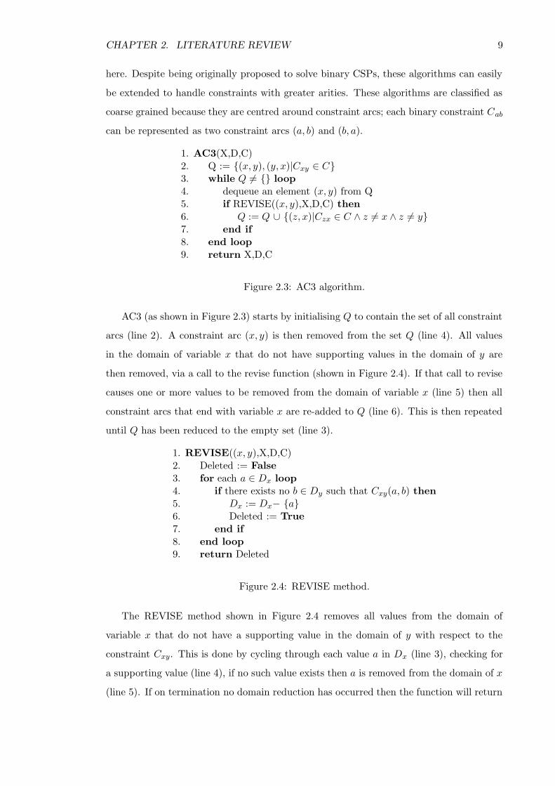
AC3 (as shown in Figure 2.3) starts by initialising Q to contain the set of all constraint
arcs (line 2). A constraint arc (x, y) is then removed from the set Q (line 4). All values
in the domain of variable x that do not have supporting values in the domain of y are
then removed, via a call to the revise function (shown in Figure 2.4). If that call to revise
causes one or more values to be removed from the domain of variable x (line 5) then all
constraint arcs that end with variable x are re-added to Q (line 6). This is then repeated
until Q has been reduced to the empty set (line 3).
1. REVISE((x, y),X,D,C)2. Deleted := False3. for each a ∈ Dx loop4. if there exists no b ∈ Dy such that Cxy(a, b) then5. Dx := Dx− a6. Deleted := True7. end if8. end loop9. return Deleted
Figure 2.4: REVISE method.
The REVISE method shown in Figure 2.4 removes all values from the domain of
variable x that do not have a supporting value in the domain of y with respect to the
constraint Cxy. This is done by cycling through each value a in Dx (line 3), checking for
a supporting value (line 4), if no such value exists then a is removed from the domain of x
(line 5). If on termination no domain reduction has occurred then the function will return
CHAPTER 2. LITERATURE REVIEW 10
the value False otherwise the value True will be returned (line 8). In the worst case, the
REVISE method will check each of the e domain values in the domain of x against the f
values in the domain of y. Both e and f are less than or equal to d. Therefore, a single
call to REVISE will run in O(d2) time.
The loop in the AC3 algorithm will loop once for each constraint arc added to the set
Q. Initially 2e constraint arcs are added to Q, where e is the number of constraints in the
CSP. Additional constraint arcs can only be added when the domain of a target variable
has values removed. A constraint arc (x, y) can, in the worse case, be re-introduced to Q
once for each of the d values in the domain of y. Therefore, a maximum of 2ed constraint
arcs can be re-introduced to Q. This means the loop will cycle O(ed) times. Each loop
will make a call to the REVISE function, which runs in O(d2) time, making the overall
worse case time complexity of a call to AC3 O(ed3).
In 2001, Bessiere et al. [21], and Zhang et al. [98], presented AC2001 and AC3.1 re-
spectively. Due to the similarity of these algorithms the authors went on to publish a
joint paper [22] that describes the algorithm named AC2001. This algorithm uses the
same basic principle as AC3 (shown in Figure 2.3). The difference between the two is
that AC2001 has an improved REVISE method. When the original REVISE method was
called to revise a constraint arc (x, y), each value in the domain of x is checked against
each value in the domain of y. In AC2001 the REVISE method stores previously found
supporting values. This enables subsequent calls to REVISE to simply check to see if the
previous supporting value is still in the domain.
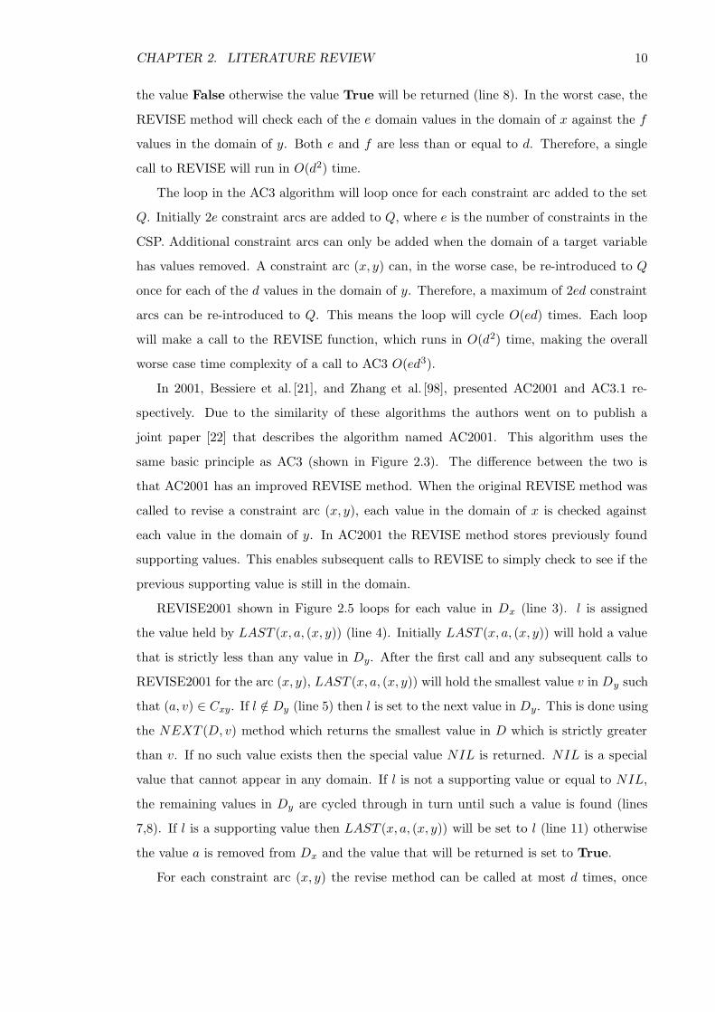
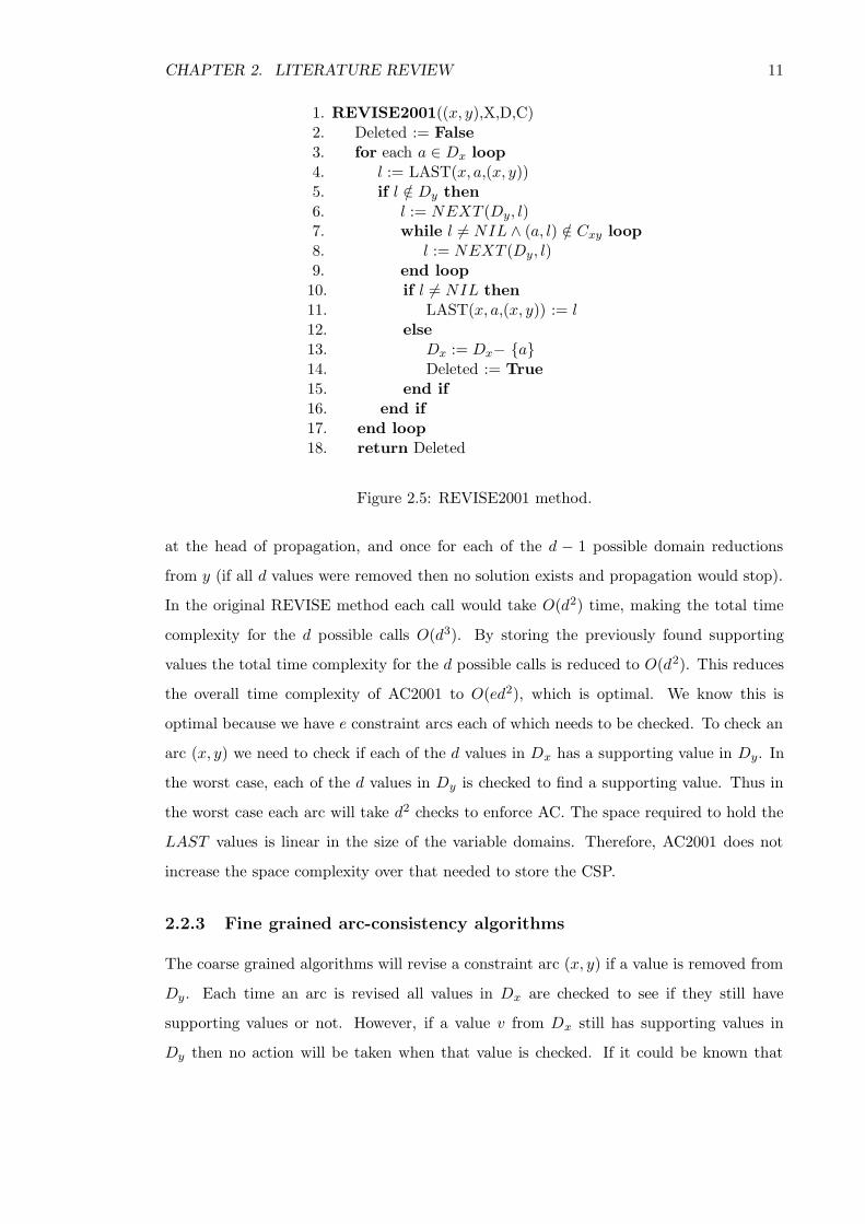
REVISE2001 shown in Figure 2.5 loops for each value in Dx (line 3). l is assigned
the value held by LAST (x, a, (x, y)) (line 4). Initially LAST (x, a, (x, y)) will hold a value
that is strictly less than any value in Dy. After the first call and any subsequent calls to
REVISE2001 for the arc (x, y), LAST (x, a, (x, y)) will hold the smallest value v in Dy such
that (a, v) ∈ Cxy. If l /∈ Dy (line 5) then l is set to the next value in Dy. This is done using
the NEXT (D, v) method which returns the smallest value in D which is strictly greater
than v. If no such value exists then the special value NIL is returned. NIL is a special
value that cannot appear in any domain. If l is not a supporting value or equal to NIL,
the remaining values in Dy are cycled through in turn until such a value is found (lines
7,8). If l is a supporting value then LAST (x, a, (x, y)) will be set to l (line 11) otherwise
the value a is removed from Dx and the value that will be returned is set to True.
For each constraint arc (x, y) the revise method can be called at most d times, once
CHAPTER 2. LITERATURE REVIEW 11
1. REVISE2001((x, y),X,D,C)2. Deleted := False3. for each a ∈ Dx loop4. l := LAST(x, a,(x, y))5. if l /∈ Dy then6. l := NEXT (Dy, l)7. while l 6= NIL ∧ (a, l) /∈ Cxy loop8. l := NEXT (Dy, l)9. end loop10. if l 6= NIL then11. LAST(x, a,(x, y)) := l12. else13. Dx := Dx− a14. Deleted := True15. end if16. end if17. end loop18. return Deleted
Figure 2.5: REVISE2001 method.
at the head of propagation, and once for each of the d − 1 possible domain reductions
from y (if all d values were removed then no solution exists and propagation would stop).
In the original REVISE method each call would take O(d2) time, making the total time
complexity for the d possible calls O(d3). By storing the previously found supporting
values the total time complexity for the d possible calls is reduced to O(d2). This reduces
the overall time complexity of AC2001 to O(ed2), which is optimal. We know this is
optimal because we have e constraint arcs each of which needs to be checked. To check an
arc (x, y) we need to check if each of the d values in Dx has a supporting value in Dy. In
the worst case, each of the d values in Dy is checked to find a supporting value. Thus in
the worst case each arc will take d2 checks to enforce AC. The space required to hold the
LAST values is linear in the size of the variable domains. Therefore, AC2001 does not
increase the space complexity over that needed to store the CSP.
2.2.3 Fine grained arc-consistency algorithms
The coarse grained algorithms will revise a constraint arc (x, y) if a value is removed from
Dy. Each time an arc is revised all values in Dx are checked to see if they still have
supporting values or not. However, if a value v from Dx still has supporting values in
Dy then no action will be taken when that value is checked. If it could be known that

CHAPTER 2. LITERATURE REVIEW 12
a supporting value still exists then that value need not be checked. The fine grained
algorithms try to address this by storing information about supporting values for each
value in each domain and only when a value’s known support set is empty is that value
checked.
In 1986 Mohr and Henderson proposed AC4 [72] the first fine grained arc-consistency
algorithm. AC4 has a pre-processing step in which it gathers support information. For
each constraint arc (x, y) and for each value in the domain of x, it finds the set of all
supporting values in the domain of y. If any values have an empty support set for any
constraint arc then that value is removed from the domain and from all support sets.
This in turn could reduce some other value’s support set to the empty set in which case
that value will also be removed. This is then repeated until all values have a non-empty
support set for each constraint arc with which their respective variables are associated.
At this point, the variable domains will have reached the same fixed point as achieved by
the course grained arc-consistency algorithms.
AC4 has an optimal worst case time complexity of O(ed2). However, because of the
computation required to produce the support sets the best case time complexity of AC4
is also Ω(ed2), thus making the complexity of AC4 Θ(ed2). The support sets also require
O(ed2) space. Due to this poor best case complexity, the sub-optimal AC3 can outper-
form AC4 on many CSP instances. For example, consider a CSP with n variables and
e constraint arcs, in which each value in each domain is supported by the first value in
any other variable’s domain (in which case enforcing AC would not remove any values).
AC3 would cycle through each of the e arcs and check each of the d values against the
first value in the connected domain, it would find that it was a supporting value and move
on. The algorithm would terminate after making ed checks. AC4 on the same CSP would
check each of the d values in the first domain against each of the d values in the second
domain, for each of the e constraints. The algorithm would then terminate after making
ed2 checks.
In 1993, Bessiere [15] proposed AC6 as an improvement on the best case performance
of AC4 whilst retaining the optimal worst case performance. Instead of computing the full
support set for each constraint arc, AC6 finds and stores only the first support value. If
that single support value is removed then an attempt to find a new support value starts
from the next value in the domain; this works in a similar way to the AC2001 REVISE
method.
CHAPTER 2. LITERATURE REVIEW 13
AC6 has the same optimal worst case time complexity as AC4, namely O(ed2). How-
ever, the best case complexity is reduced to O(ed), which is the same as that of AC3. The
space complexity is also reduced to O(ed).
In 1999, Bessiere et al. proposed AC7 [17], which improves on AC6 by exploiting the
bidirectional nature of support values over a binary constraint, meaning that (a, b) ∈ Cxy
iff (b, a) ∈ Cyx. AC7 uses this knowledge by inferring support for some domain values
instead of searching for one. For example, for a constraint arc (x, y), if value v2 from Dy
was found to support the value v1 from Dx, then when the arc (y, x) is processed, instead
of searching for a support value for v2, AC7 would infer that v1 was a supporting value.
AC7 has the same time complexities as AC6, namely O(ed2) in the worst case and
O(ed) in the best. However, in practice AC7 can significantly reduce the number of checks
required, which provides a reasonable time reduction.
2.2.4 Generic algorithms
Both the coarse and fine grained algorithms require each constraint to have a function
which returns True if the value v1 in Dx is consistent with the value v2 in Dy, otherwise
it must return False. This leaves little room to exploit any constraint specific knowledge.
For example, a constraint x > y where Dx = 1, 2, 3 and Dy = 4, 5, 6 is clearly
unsatisfiable, however all previously mentioned AC algorithms would require at least nine
constraint checks to discover this. For this constraint the arc (x, y) could be found to be
unsatisfiable with only one check, by comparing the smallest value in Dy with the largest
value in Dx.
In 1992, Van Hentenryck et al. proposed AC5 [96] to exploit the structures of different
classes of constraints. In the course grained algorithms the Q object contains constraint
arcs to be revised, whilst in the fine grained algorithms, Q contains pairs (xi, a) where xi
is a variable and a is a value that has been removed from Di. In AC5, Q contains elements
〈(x, y), a〉 where (x, y) is a constraint arc and a is a value removed from Dy.
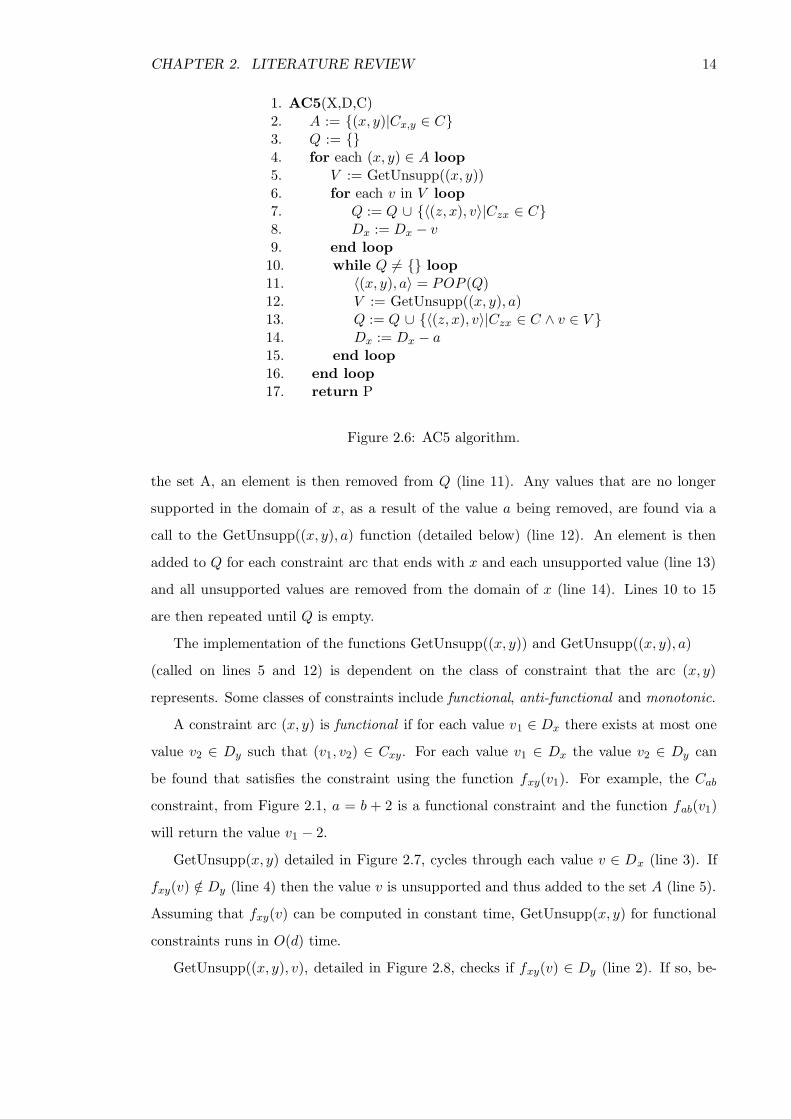
In AC5, shown in Figure 2.6, all constraint arcs are first placed in a set A (line 2),
the Q object is initialised to the empty set (line 3). For each arc in the set A (line 4) all
the unsupported values in the domain of x are found via a call to the GetUnsupp((x, y))
function (detailed in Figure 2.7) (line 5). An element is then added to Q for each constraint
arc that ends with x and each unsupported value (line 7), and all unsupported values are
removed from the domain of x (line 8). After all constraint arcs have been removed from
CHAPTER 2. LITERATURE REVIEW 14
1. AC5(X,D,C)2. A := (x, y)|Cx,y ∈ C3. Q := 4. for each (x, y) ∈ A loop5. V := GetUnsupp((x, y))6. for each v in V loop7. Q := Q ∪ 〈(z, x), v〉|Czx ∈ C8. Dx := Dx − v9. end loop
10. while Q 6= loop11. 〈(x, y), a〉 = POP (Q)12. V := GetUnsupp((x, y), a)13. Q := Q ∪ 〈(z, x), v〉|Czx ∈ C ∧ v ∈ V 14. Dx := Dx − a15. end loop16. end loop17. return P
Figure 2.6: AC5 algorithm.
the set A, an element is then removed from Q (line 11). Any values that are no longer
supported in the domain of x, as a result of the value a being removed, are found via a
call to the GetUnsupp((x, y), a) function (detailed below) (line 12). An element is then
added to Q for each constraint arc that ends with x and each unsupported value (line 13)
and all unsupported values are removed from the domain of x (line 14). Lines 10 to 15
are then repeated until Q is empty.
The implementation of the functions GetUnsupp((x, y)) and GetUnsupp((x, y), a)
(called on lines 5 and 12) is dependent on the class of constraint that the arc (x, y)
represents. Some classes of constraints include functional, anti-functional and monotonic.
A constraint arc (x, y) is functional if for each value v1 ∈ Dx there exists at most one
value v2 ∈ Dy such that (v1, v2) ∈ Cxy. For each value v1 ∈ Dx the value v2 ∈ Dy can
be found that satisfies the constraint using the function fxy(v1). For example, the Cab
constraint, from Figure 2.1, a = b + 2 is a functional constraint and the function fab(v1)
will return the value v1 − 2.
GetUnsupp(x, y) detailed in Figure 2.7, cycles through each value v ∈ Dx (line 3). If
fxy(v) /∈ Dy (line 4) then the value v is unsupported and thus added to the set A (line 5).
Assuming that fxy(v) can be computed in constant time, GetUnsupp(x, y) for functional
constraints runs in O(d) time.
GetUnsupp((x, y), v), detailed in Figure 2.8, checks if fxy(v) ∈ Dy (line 2). If so, be-

CHAPTER 2. LITERATURE REVIEW 15
1. GetUnsupp((x, y))2. A := 3. for each v ∈ Dx loop4. if fxy(v) /∈ Dy then5. A := A ∪ v6. end if7. end loop8. return A
Figure 2.7: GetUnsupp((x, y)) method for functional constraints
1. GetUnsupp((x, y),v)2. if fxy(v) ∈ Dy then3. return fxy(v)4. else5. return 6. end if
Figure 2.8: GetUnsupp((x, y),v) method for functional constraints
cause its only supporting value in Dx has been removed fxy(v) is no longer supported.
Assuming that fxy(v) can be computed in constant time, GetUnsupp((x, y), v) for func-
tional constraints runs in O(1) time. Therefore, AC can be enforced on a CSP containing
only functional constraints in O(ed) time.
A constraint arc (x, y) is anti-functional if the negation of the constraint is functional,
meaning that for each value v1 ∈ Dx there exists at most one value v2 ∈ Dy such that
(v1, v2) /∈ Cxy. For example, the Cbc (b 6= c) constraint, from Figure 2.1, is an anti-
functional constraint. The function fbc(v1) returns the single value that would not support
v1 which, in this case, is v1.
1. GetUnsupp((x, y))2. s := SIZE(Dy)3. m := MIN(Dy)4. if (s = 1) ∧ (fxy(m) ∈ Dx) then5. return fxy(m)6. else7. return 8. end if
Figure 2.9: GetUnsupp((x, y)) method for anti-functional constraints
In the GetUnsupp((x, y)) method for anti-functional constraints (Figure 2.9) the
SIZE(Dy) method returns |Dy|, and MIN(Dy) returns the smallest value in Dy. All values
CHAPTER 2. LITERATURE REVIEW 16
v1 ∈ Dy support all but one value v2 ∈ Dx. The value v2 that v1 does not support is
different for each v1. Therefore, if Dy contains more than one value then all values in
Dx are supported. If Dy does contain only one value (line 4) and the value fyx(m) ∈ Dx
(line 4) then the only unsupported value is fxy(m). Since this method contains no loops,
and assuming fxy(m) runs in constant time, then GetUnsupp((x, y)) for anti-functional
constraints runs in O(1) time.
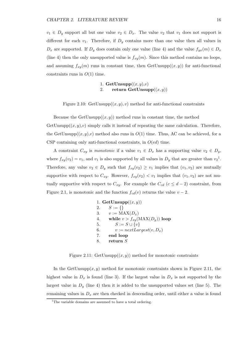
1. GetUnsupp((x, y),v)2. return GetUnsupp((x, y))
Figure 2.10: GetUnsupp((x, y), v) method for anti-functional constraints
Because the GetUnsupp((x, y)) method runs in constant time, the method
GetUnsupp((x, y),v) simply calls it instead of repeating the same calculation. Therefore,
the GetUnsupp((x, y),v) method also runs in O(1) time. Thus, AC can be achieved, for a
CSP containing only anti-functional constraints, in O(ed) time.
A constraint Cxy is monotonic if a value v1 ∈ Dx has a supporting value v2 ∈ Dy,
where fxy(v2) = v1, and v1 is also supported by all values in Dy that are greater than v21.
Therefore, any value v2 ∈ Dy such that fxy(v2) ≥ v1 implies that (v1, v2) are mutually
supportive with respect to Cxy. However, fxy(v2) < v1 implies that (v1, v2) are not mu-
tually supportive with respect to Cxy. For example the Ccd (c ≤ d − 2) constraint, from
Figure 2.1, is monotonic and the function fcd(v) returns the value v − 2.
1. GetUnsupp((x, y))2. S := 3. v := MAX(Dx)4. while v > fxy(MAX(Dy)) loop5. S := S ∪ v6. v := nextLargest(v,Dx)7. end loop8. return S
Figure 2.11: GetUnsupp((x, y)) method for monotonic constraints
In the GetUnsupp(x, y) method for monotonic constraints shown in Figure 2.11, the
highest value in Dx is found (line 3). If the largest value in Dx is not supported by the
largest value in Dy (line 4) then it is added to the unsupported values set (line 5). The
remaining values in Dx are then checked in descending order, until either a value is found
1The variable domains are assumed to have a total ordering.

CHAPTER 2. LITERATURE REVIEW 17
that is supported by the largest value in Dy or all values have been checked.
1. GetUnsupp((x, y),v)2. if v > MAX(Dy)3. return GetUnsupp(x, y)4. else5. return 6. end if
Figure 2.12: GetUnsupp((x, y),v) method for monotonic constraints
The GetUnsupp((x, y), v) method shown in Figure 2.12 assumes that, prior to the value
v being removed from Dy, all values in Dx were supported by the largest value in Dy, which
would be the case after the set of unsupported values identified by the GetUnsupp(x, y)
method have been removed from Dx. The removed value is then checked against the
highest remaining value in Dy. If it is greater than the current largest value then the new
set of unsupported values are found via a call to GetUnsupp(x, y).
It is important to note that the discussed methods for monotonic constraints will only
work with the (x, y) arc from a constraint Cxy. To process the (y, x) constraint arc we
require the symmetric equivalent of the discussed methods. In this case, instead of checking
the largest values from the domains the smallest values will be compared.
As with functional and anti-functional constraints a CSP containing only monotonic
constraints can be made arc-consistent in O(ed) time. This is assuming that the variables
are represented in such a way as to allow the bounds of a variable to be changed in constant
time, such as the variable representation detailed in [96].
In 2005, Jean-Charles Regin proposed AC-* [80] a configurable, generic and adaptive
arc-consistency algorithm. In this publication, the author details the elements which make
up each of the previously published arc-consistency algorithms and shows how AC-* can
be configured to use any combination of these elements. This algorithm can also be re-
configured mid-search.
2.2.5 Constraint solvers
The early constraint solvers, such as CHIP [95], CLP [52], Sicstus [6] and Eclipse [7],
were mostly written as extensions of the Prolog programming language. These solvers had
a “black box” approach, meaning that the constraint implementations, search processes
and propagation algorithms are hidden. This approach limits the user’s ability to take

CHAPTER 2. LITERATURE REVIEW 18
advantage of problem specific knowledge to improve the constraint model.
More recent constraint solvers such as Ilog solver [3], Koalog solver [5], JChoco [4] and
Gecode [1] take more of a “glass box” approach [78]. All these solvers are implemented as
a library for an object-oriented programming language (Java, C++ or C#). By making
use of inheritance, these constraint solvers provide the basic frame-work within which
different components can be combined and configured, to construct a constraint model.
The resulting constraint model can then be propagated by the solver’s built in propagation
algorithm, which is based on the generic AC5 [96] arc-consistency algorithm. This type of
frame-work allows users to implement their own constraints by providing a basic interface
which can be extended to produce a constraint class. To implement a constraint in this way,
the user is required to write methods that will be called during propagation. At least two
methods are required to implement a constraint. One is called at the head of propagation
and the other is called when the domain of one of the constrained variables is reduced.
These methods will then query the variable domains and remove any inconsistent domain
values by interacting with the variable objects directly. The solver may also require the user
to state when the constraint is to be propagated, namely when a variable is instantiated
(the variable domain is reduced to a singleton), when the bounds of a variable domain are
altered, or when any domain reduction occurs.
Not all recent constraint solvers follow the “glass box” approach. In 2006, Gent et al.
proposed Minion [41] a light-weight efficient solver implemented in C++. Minion takes
the definition of a CSP as input, solves the problem then outputs the results. This solver
has no provision for user-defined constraints.
2.2.6 Global constraints
Global constraints [19] are constraints with an arity n where n is a parameter. They are
used to represent an entire problem or sub-problem in a single constraint. The main moti-
vation behind global constraints is to improve either efficiency or the level of propagation
attained. One such example is the AllDifferent constraint proposed by Regin [79]. The
AllDifferent constraint posted over a set of variables X will ensure that all the variables
in X are assigned different values. The same effect can be achieved by posting the set
of constraints xi 6= xj |i 6= j, xi ∈ X,xj ∈ X. In this case Regin’s AllDifferent con-
straint will achieve a higher level of consistency over the variables. However, propagating
Regin’s constraint has a higher time complexity than that of enforcing arc-consistency
CHAPTER 2. LITERATURE REVIEW 19
over the set of not-equal constraints. Other propagation methods have been proposed for
the AllDifferent constraint that have a lower time complexity, but enforce a lower level
of consistency [71]. Other examples of global constraints include the flow constraint [23]
written to help model the network flow problem, and the slide constraint [18] written to
help model scheduling problems.
2.3 Stable matching problems
In this section, the classical stable marriage problem is defined along with an optimal
algorithm that is guaranteed to find a solution. Generalisations of the problem are also
given, which include: ties, incomplete preference lists, the Hospitals/Residents problem
and the Stable Roommates problem.
2.3.1 The Stable Marriage problem
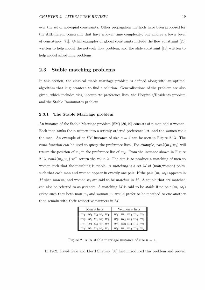
An instance of the Stable Marriage problem (SM) [36,49] consists of n men and n women.
Each man ranks the n women into a strictly ordered preference list, and the women rank
the men. An example of an SM instance of size n = 4 can be seen in Figure 2.13. The
rank function can be used to query the preference lists. For example, rank(m2, w1) will
return the position of w1 in the preference list of m2. From the instance shown in Figure
2.13, rank(m2, w1) will return the value 2. The aim is to produce a matching of men to
women such that the matching is stable. A matching is a set M of (man,woman) pairs,
such that each man and woman appear in exactly one pair. If the pair (mi, wj) appears in
M then man mi and woman wj are said to be matched in M . A couple that are matched
can also be referred to as partners. A matching M is said to be stable if no pair (mi, wj)
exists such that both man mi and woman wj would prefer to be matched to one another
than remain with their respective partners in M .
Men’s lists Women’s lists
m1: w1 w3 w2 w4 w1: m1 m3 m2 m4
m2: w4 w1 w2 w3 w2: m2 m4 m1 m3
m3: w1 w4 w3 w2 w3: m3 m4 m2 m1
m4: w3 w4 w2 w1 w4: m1 m3 m4 m2
Figure 2.13: A stable marriage instance of size n = 4.
In 1962, David Gale and Lloyd Shapley [36] first introduced this problem and proved

CHAPTER 2. LITERATURE REVIEW 20
that all problem instances admit at least one stable matching. This was done by describing
an algorithm, referred to as the Gale/Shapley (GS) algorithm, which is guaranteed to find
a stable matching for any given problem instance. Furthermore, this algorithm is known to
be optimal [74]; it finds a stable matching in time linear in the size of the problem instance,
i.e. in O(n2) time [60]. The GS algorithm can be run with two different orientations. One
favours the men and the other favours the women. This algorithm was later refined to
give the Extended Gale/Shapley (EGS) algorithm [49].
Figure 2.14 shows the man-oriented version of the extended Gale/Shapley (EGS) al-
gorithm. Initially, all men are added to the free list (line 1). An arbitrary man m is then
picked from the free list and he makes a proposal to his most preferred woman w (line 3).
If w was previously engaged (line 4) then her previous fiance will be placed back in the
free list (line 5). Man m and woman w will then be engaged (line 7). Then all men that
appear after m in w’s preference list are removed (line 9) and w will also be removed from
their preference lists (line 10). This is then repeated until the free list is empty (line 2).
1. assign each person to be free2. while some man m is free loop3. w := first woman on m’s list4. if some man p is engaged to w then5. assign p to be free6. end if7. assign m and w to be engaged to each other8. for each successor p of m on w’s list loop9. delete p from w’s list
10. delete w from p’s list11. end loop12. end loop
Figure 2.14: The man-oriented Extended Gale/Shapley algorithm.
On termination of the EGS algorithm the preference lists will have been reduced to a
fixed point, meaning that running the algorithm again over these reduced preference lists
will not reduce them further. These reduced preference lists are known as the MGS-lists
(the Man-oriented Gale/Shapley lists). If all men are matched to their first choice woman
from the MGS-lists then the matching will be stable. The matching will also be man-
optimal and woman-pessimal. This means that each man is matched to his best possible
partner in any stable matching and each woman is matched to her worst possible partner in
any stable matching. If the algorithm is run with the men and women swapped, giving the
CHAPTER 2. LITERATURE REVIEW 21
woman-oriented EGS algorithm, then the reduced preference lists produced after applying
this algorithm will be the WGS-lists (the Woman-oriented Gale/Shapley lists). If all the
women are matched to their first choice in the WGS-lists then that matching will be the
woman-optimal and man-pessimal stable matching. The intersection of the MGS-lists and
the WGS-lists is known as the GS-lists. The GS-lists can also be found by applying the
woman-oriented algorithm to the MGS-lists or the man-oriented algorithm to the WGS-
lists. The GS-lists contain all possible stable matchings [37].
A full proof of correctness is without of the scope of this document, however, a brief
justification of correctness is now given. If each man is matched to the first woman in
their MGS-list then the matching will be a bijection. For this not to be the case then two
men mi and mk must have the same woman wj at the head of their MGS-list. Assuming
that rank(wj ,mi) < rank(wj,mk), at some point mi and wj must have been engaged,
at which time wj would have been removed from mk’s list, which is a contradiction. If
mi is matched to the first woman in his preference list wj , then (mi, wk) will not form a
blocking pair, where (k 6= j). This is because if mi prefers wj to wk then they cannot
form a blocking pair or if mi prefers wk to wj then wk must have been removed from mi’s
list when she received a proposal from someone she preferred to mi, meaning she must be
matched to someone she prefers to mi, and thus, they cannot form a blocking pair.
2.3.2 Incomplete preference lists
The Stable Marriage problem with Incomplete preference lists (SMI) is a generalisation
of the classical stable marriage problem. By allowing preference lists to be incomplete,
participants in a matching are allowed to express the fact that they would rather not have
a partner than be matched to someone that has been omitted from their preference list.
This generalisation requires an extension to the definitions of a matching and of stability.
A matching is a set M of (man,woman) acceptable pairs, such that each man and woman
appear in at most one pair. A pair (mi, wj) is acceptable iff mi and wj appear in each
others preference lists. A matching M for an instance of SMI is stable iff it contains no
blocking pair (mi, wj). The pair (mi, wj) will form a blocking pair if it is acceptable, mi
is either unmatched in M or prefers wj to his partner in M and wj is either unmatched
in M or prefers mi to her partner in M . Note that, in SMI with the extended definition
of stability, there is no longer any need to assume that the number of men and women are
equal.
CHAPTER 2. LITERATURE REVIEW 22
All instances of SMI admit at least one stable matching. However, this matching may
not be complete, meaning that some participants may not be matched. It has been proven
that the set of unmatched participants is the same for all stable matchings for a given
instance of SMI [37].
A stable matching can be found for an instance of SMI in O(L) time by using the EGS
algorithm, where L is the sum of the lengths of the preference lists.
2.3.3 Ties in preference lists
The Stable Marriage problem with Ties (SMT) allows participants in a matching to express
indifference between two or more potential partners. This relaxation gives rise to three
extensions of the classical definition of stability. In all three extensions a matching is stable
iff it contains no blocking pair; the definitions differ in what constitutes a blocking pair.
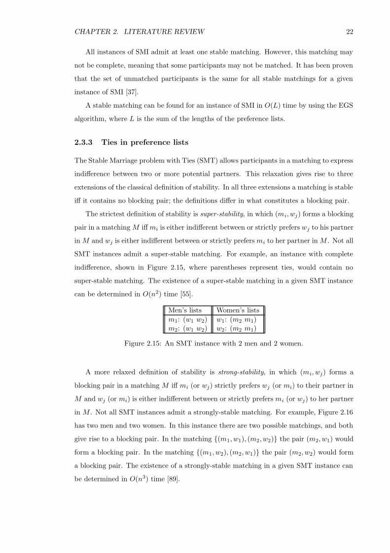
The strictest definition of stability is super-stability, in which (mi, wj) forms a blocking
pair in a matching M iff mi is either indifferent between or strictly prefers wj to his partner
in M and wj is either indifferent between or strictly prefers mi to her partner in M . Not all
SMT instances admit a super-stable matching. For example, an instance with complete
indifference, shown in Figure 2.15, where parentheses represent ties, would contain no
super-stable matching. The existence of a super-stable matching in a given SMT instance
can be determined in O(n2) time [55].
Men’s lists Women’s lists
m1: (w1 w2) w1: (m2 m1)m2: (w1 w2) w2: (m2 m1)
Figure 2.15: An SMT instance with 2 men and 2 women.
A more relaxed definition of stability is strong-stability, in which (mi, wj) forms a
blocking pair in a matching M iff mi (or wj) strictly prefers wj (or mi) to their partner in
M and wj (or mi) is either indifferent between or strictly prefers mi (or wj) to her partner
in M . Not all SMT instances admit a strongly-stable matching. For example, Figure 2.16
has two men and two women. In this instance there are two possible matchings, and both
give rise to a blocking pair. In the matching (m1, w1), (m2, w2) the pair (m2, w1) would
form a blocking pair. In the matching (m1, w2), (m2, w1) the pair (m2, w2) would form
a blocking pair. The existence of a strongly-stable matching in a given SMT instance can
be determined in O(n3) time [89].

CHAPTER 2. LITERATURE REVIEW 23
Men’s lists Women’s lists
m1: w1 w2 w1: m2 m1
m2: (w1 w2) w2: m2 m1
Figure 2.16: An SMT instance with 2 men and 2 women.
The third definition of stability is weak-stability, in which (mi, wj) forms a blocking
pair in a matching M only if both mi and wj strictly prefer each other to their partners
in M . All instances of SMT admit at least one weakly-stable matching. A weakly-stable
matching can be found in an SMT instance by arbitrarily breaking the ties and applying
the EGS algorithm [49].
2.3.4 Ties and incomplete preference lists
The Stable Marriage problem with Ties and Incomplete preferences (SMTI) is a fur-
ther generalisation of the classical stable marriage problem. To extend the definitions of
super-stability, strong-stability and weak-stability to allow for incomplete preference lists,
unmatched people need to be considered.
• Under super-stability, a pair (mi, wj) forms a blocking pair in a matching M iff they
are an acceptable pair, mi is either indifferent between or strictly prefers wj to his
partner in M or mi is unmatched in M and wj is either indifferent between or strictly
prefers mi to her partner in M or wj is unmatched in M .
• Under strong-stability, a pair (mi, wj) forms a blocking pair in a matching M iff
they are an acceptable pair, mi (or wj) strictly prefers wj (or mi) to their partner
in M or mi (or wj) is unmatched in M and wj (or mi) is either indifferent between
or strictly prefers mi (or wi) to her partner in M or wj (or mi) is unmatched in M .
• Under weak-stability, a pair (mi, wj) forms a blocking pair in a matching M iff they
are an acceptable pair and both mi and wj strictly prefer each other to their partners
in M or are unmatched in M .
A stable matching for such an instance under super-stability and strong-stability can
be found in polynomial time [65] if such a matching exists. Under weak-stability a stable
matching can be found by arbitrarily breaking the ties and applying the EGS algorithm.
However, under weak-stability it is no longer the case that all stable matchings have the
same size or the same set of participants matched. The SMTI instance given in Figure

CHAPTER 2. LITERATURE REVIEW 24
2.17 admits two stable matchings. The first, (m1, w1), has m1 and w1 matched to each
other while m2 and w2 are unmatched. In the other matching, (m1, w2), (m2, w1), all
participants are matched.
Men’s lists Women’s lists
m1: (w1 w2) w1: (m1 m2)m2: w1 w2: m1
Figure 2.17: An SMTI instance with 2 men and 2 women.
It can be advantageous in a matching scheme, that allows both ties and incomplete
preferences, to find a weakly stable matching in which the maximum number of participants
is matched. It has been proven [58,66] to be NP-hard to find a maximum cardinality weakly
stable matching for an instance of SMTI.
2.3.5 Hospitals/Residents problem
The Hospitals/Residents problem (HR) [36]2 is a many-to-one stable matching problem.
There are a set of n residents (medical students) each wishing to be assigned to a post at
one of m hospitals. Each resident ranks a subset of the hospitals into a strictly ordered
preference lists, similarly, all hospitals will rank a subset of the residents. Each hospital
hj can have zero, one or more residents assigned to it up to a maximum of cj , where hj
has cj available posts. The objective is to find a matching of residents to hospitals such
that each resident is matched to only one hospital, the hospital capacities are respected
and the matching is stable. A matching M is stable if it contains no blocking pairs. A
(resident,hospital) pair (ri, hj) form a blocking pair if the three following conditions are
met:
• (ri, hj) is not in M but is an acceptable pair.
• ri is unassigned in M or prefers hj to its assigned hospital in M .
• either hj has less than c residents assigned to it or hj prefers ri to at least one of its
assigned residents in M .
Note that a special case of this problem, in which all hospital capacities equal one and
n = m, is equivalent to SMI.
2referred to in this paper as the college admissions problem.
CHAPTER 2. LITERATURE REVIEW 25
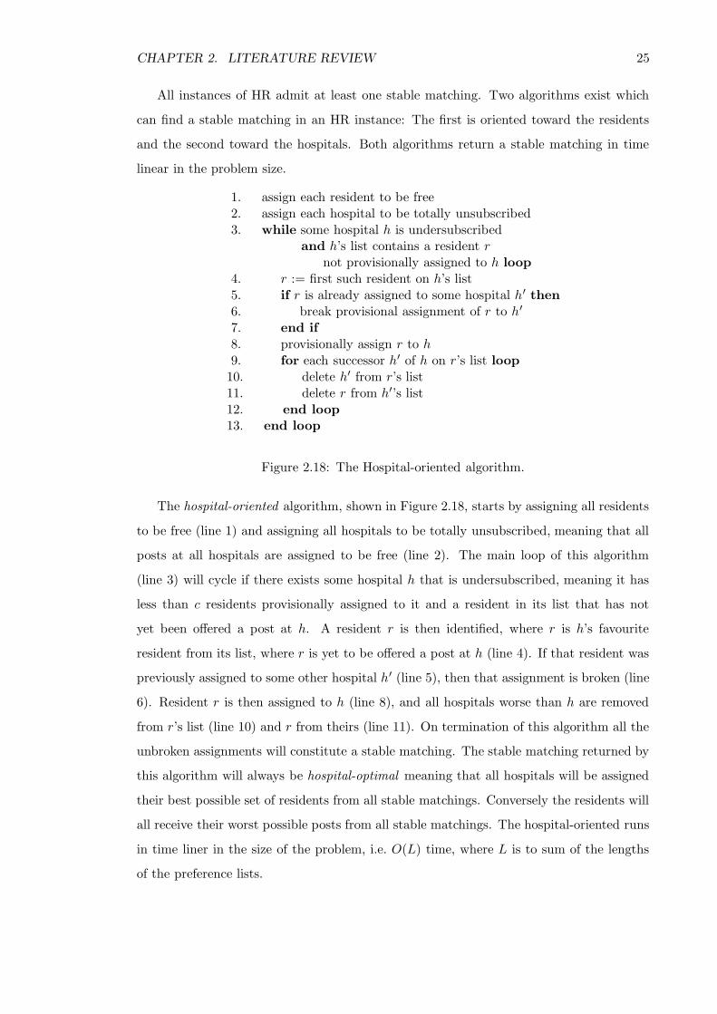
All instances of HR admit at least one stable matching. Two algorithms exist which
can find a stable matching in an HR instance: The first is oriented toward the residents
and the second toward the hospitals. Both algorithms return a stable matching in time
linear in the problem size.
1. assign each resident to be free2. assign each hospital to be totally unsubscribed3. while some hospital h is undersubscribed
and h’s list contains a resident rnot provisionally assigned to h loop
4. r := first such resident on h’s list5. if r is already assigned to some hospital h′ then6. break provisional assignment of r to h′
7. end if8. provisionally assign r to h9. for each successor h′ of h on r’s list loop10. delete h′ from r’s list11. delete r from h′’s list12. end loop13. end loop
Figure 2.18: The Hospital-oriented algorithm.
The hospital-oriented algorithm, shown in Figure 2.18, starts by assigning all residents
to be free (line 1) and assigning all hospitals to be totally unsubscribed, meaning that all
posts at all hospitals are assigned to be free (line 2). The main loop of this algorithm
(line 3) will cycle if there exists some hospital h that is undersubscribed, meaning it has
less than c residents provisionally assigned to it and a resident in its list that has not
yet been offered a post at h. A resident r is then identified, where r is h’s favourite
resident from its list, where r is yet to be offered a post at h (line 4). If that resident was
previously assigned to some other hospital h′ (line 5), then that assignment is broken (line
6). Resident r is then assigned to h (line 8), and all hospitals worse than h are removed
from r’s list (line 10) and r from theirs (line 11). On termination of this algorithm all the
unbroken assignments will constitute a stable matching. The stable matching returned by
this algorithm will always be hospital-optimal meaning that all hospitals will be assigned
their best possible set of residents from all stable matchings. Conversely the residents will
all receive their worst possible posts from all stable matchings. The hospital-oriented runs
in time liner in the size of the problem, i.e. O(L) time, where L is to sum of the lengths
of the preference lists.

CHAPTER 2. LITERATURE REVIEW 26
1. assign each resident to be free2. assign each hospital to be totally unsubscribed3. while some resident r is free
and r has a nonempty list loop4. h := first hospital on r’s list5. if h is fully subscribed then6. r′ := worst resident provisionally assigned to h7. assign r′ to be free8. end if9. provisionally assign r to h10. if h is fully subscribed then11. s := worst resident provisionally assigned to h12. for each successor s′ of s on h’s list loop13. delete s′ from h’s list14. delete h from s′’s list15. end loop16. end if17. end loop
Figure 2.19: The Resident-oriented algorithm.
The resident-oriented algorithm shown in Figure 2.19 starts by assigning all residents
to be free (line 1) and assigning all hospital posts to be free (line 2). The main loop
of this algorithm (line 3) will cycle if there exists some resident r that is free and has a
non-empty preference list. Resident r’s favourite hospital h currently remaining in its list
is found (line 4). If h is fully subscribed, meaning that is has c residents provisionally
assigned to it, (line 5) then its least favourite resident that is currently assigned to it is
assigned to be free (line 7) and r is assigned to h (line 9). If h is now fully subscribed (line
10) then all residents worse than h’s least favourite assigned resident (lines 11,12) must be
removed from h’s list (line 13) and h must be removed from their list (line 14). As with the
hospital-oriented algorithm, on termination of this algorithm all the unbroken assignments
will constitute a stable matching. The stable matching returned by this algorithm will
always be resident-optimal. This means that all residents will receive their best possible
hospital posts from all stable matchings. The resident-oriented runs in time liner in the
size of the problem, i.e. O(L) time, where L is to sum of the lengths of the preference lists.
A generalisation of HR is the Hospitals/Residents problem with ties (HRT). As with
SMT, there are three different definitions of a blocking pair.
• Under super-stability, a pair (r, h) forms a blocking pair in a matching M iff they are
an acceptable pair, r is either indifferent between or strictly prefers h to his assigned

CHAPTER 2. LITERATURE REVIEW 27
hospital in M or r is unmatched in M and h is either indifferent between or strictly
prefers r to its worst assigned resident in M or h is not fully subscribed in M .
• Under strong-stability, a pair (r, h) forms a blocking pair in a matching M iff they
are an acceptable pair, r (or h) strictly prefers h (or r) to his assigned hospital (worst
assigned resident) in M or r (or h) is unmatched (not fully subscribed) in M and h
(or r) is either indifferent between or strictly prefers r (or h) to its worst assigned
resident (assigned hospital) in M or h (or r) is not fully subscribed (unmatched) in
M .
• Under weak-stability, a pair (r, h) forms a blocking pair in a matching M iff they
are an acceptable pair, r strictly prefers h to his assigned hospital in M or is un-
matched in M , and h strictly prefers r to its worst assigned resident in M , or is
undersubscribed.
Under super-stability a stable matching can be found in O(L) time [54] and under
strong-stability a matching can be found in O(cL) time [89], where c is the sum of all
hospital capacities. Under weak-stability a stable matching can be found by arbitrarily
breaking the ties and applying either the resident-oriented or hospital-oriented algorithms
defined above.
HR is a “real world” problem handled by centralised matching schemes. Such match-
ing schemes include the National Resident Matching Program (NRMP) in the United
States [73]. The NRMP has been in operation since 1952 and handles the annual alloca-
tion of around 31,000 residents to about 2,300 hospitals. Other matching schemes include
the Canadian Resident Matching Service (CaRMS) [27] and the Scottish Foundation Al-
location Scheme (SFAS) [56].
2.3.6 Stable Roommates problem
The Stable Roommates problem (SR) [36] is a matching problem in which there is a single
set of participants of even size. Each person wishes to be assigned a room, each room
has a capacity of two, thus the set of participants must be split into pairs. Each person
strictly ranks all others into a preference list. The objective is to find a matching M which
is stable. A matching is a set of pairs (roommate,roommate), such that each participant
appears in at most one pair, and the two roommates are distinct. A matching M is stable
if it admits no blocking pair (ri, rk). A pair (ri, rk) will form a blocking pair in M iff
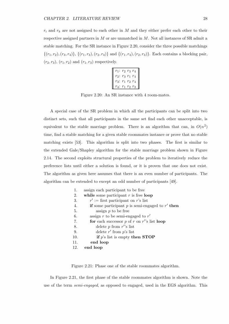
CHAPTER 2. LITERATURE REVIEW 28
ri and rk are not assigned to each other in M and they either prefer each other to their
respective assigned partners in M or are unmatched in M . Not all instances of SR admit a
stable matching. For the SR instance in Figure 2.20, consider the three possible matchings
(r1, r2), (r3, r4), (r1, r3), (r2, r4) and (r1, r4), (r2, r3). Each contains a blocking pair,
(r2, r3), (r1, r2) and (r1, r3) respectively.
r1: r2 r3 r4
r2: r3 r1 r4
r3: r1 r2 r4
r4: r1 r2 r3
Figure 2.20: An SR instance with 4 room-mates.
A special case of the SR problem in which all the participants can be split into two
distinct sets, such that all participants in the same set find each other unacceptable, is
equivalent to the stable marriage problem. There is an algorithm that can, in O(n2)
time, find a stable matching for a given stable roommates instance or prove that no stable
matching exists [53]. This algorithm is split into two phases. The first is similar to
the extended Gale/Shapley algorithm for the stable marriage problem shown in Figure
2.14. The second exploits structural properties of the problem to iteratively reduce the
preference lists until either a solution is found, or it is proven that one does not exist.
The algorithm as given here assumes that there is an even number of participants. The
algorithm can be extended to except an odd number of participants [49].
1. assign each participant to be free2. while some participant r is free loop3. r′ := first participant on r’s list4. if some participant p is semi-engaged to r ′ then5. assign p to be free6. assign r to be semi-engaged to r′
7. for each successor p of r on r′’s list loop8. delete p from r′’s list9. delete r′ from p’s list10. if p’s list is empty then STOP11. end loop12. end loop
Figure 2.21: Phase one of the stable roommates algorithm.
In Figure 2.21, the first phase of the stable roommates algorithm is shown. Note the
use of the term semi-engaged, as opposed to engaged, used in the EGS algorithm. This
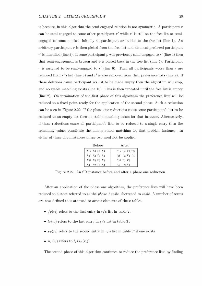
CHAPTER 2. LITERATURE REVIEW 29
is because, in this algorithm the semi-engaged relation is not symmetric. A participant r
can be semi-engaged to some other participant r ′ while r′ is still on the free list or semi-
engaged to someone else. Initially all participant are added to the free list (line 1). An
arbitrary participant r is then picked from the free list and his most preferred participant
r′ is identified (line 3). If some participant p was previously semi-engaged to r ′ (line 4) then
that semi-engagement is broken and p is placed back in the free list (line 5). Participant
r is assigned to be semi-engaged to r ′ (line 6). Then all participants worse than r are
removed from r′’s list (line 8) and r′ is also removed from their preference lists (line 9). If
these deletions cause participant p’s list to be made empty then the algorithm will stop,
and no stable matching exists (line 10). This is then repeated until the free list is empty
(line 2). On termination of the first phase of this algorithm the preference lists will be
reduced to a fixed point ready for the application of the second phase. Such a reduction
can be seen in Figure 2.22. If the phase one reductions cause some participant’s list to be
reduced to an empty list then no stable matching exists for that instance. Alternatively,
if these reductions cause all participant’s lists to be reduced to a single entry then the
remaining values constitute the unique stable matching for that problem instance. In
either of these circumstances phase two need not be applied.
Before After
r1: r4 r2 r3 r1: r4 r2 r3
r2: r3 r1 r4 r2: r3 r1 r4
r3: r4 r1 r2 r3: r1 r2
r4: r2 r1 r3 r4: r2 r1
Figure 2.22: An SR instance before and after a phase one reduction.
After an application of the phase one algorithm, the preference lists will have been
reduced to a state referred to as the phase 1 table, shortened to table. A number of terms
are now defined that are used to access elements of these tables.
• fT (ri) refers to the first entry in ri’s list in table T .
• lT (ri) refers to the last entry in ri’s list in table T .
• sT (ri) refers to the second entry in ri’s list in table T if one exists.
• nT (ri) refers to lT (sT (ri)).
The second phase of this algorithm continues to reduce the preference lists by finding

CHAPTER 2. LITERATURE REVIEW 30
and removing rotations. A rotation P is a cyclic list of pairs of participants, which takes
the form P = (p0, q0), (p1, q1), . . . , (pl−1, ql−1), where l is the length of the rotation. Each
pair in the list (pi, qi), has the property that qi = fT (pi). The relation between the pairs
in the list is such that qi+1 = sT (pi). The removal of a rotation from the table requires
that for each (pi, qi) pair in the rotation, all participants that qi likes less than pi−1 are
removed from qi’s preference list, and qi is also removed from their lists. Details of how a
rotation can be found are in [49].
1. while some list in T has more than one entry andno list in T empty list loop
2. find a rotation P3. remove P from T7. end loop
Figure 2.23: Phase two of the stable roommates algorithm.
The second phase of the roommates algorithm is shown in Figure 2.23. While some
participant has more than one list entry and no participants have an empty list this phase
will continue (line 1). A rotation P is found (line 2) rotation P is removed from T (line
3). On termination of the second phase of this algorithm, the preference lists will be in
one of two states. Either all participant’s lists have been reduced to a single entry, which
will constitute a stable matching, or some participant’s list will have been reduced to the
empty set, in which case no stable matching exists. This algorithm has been proven to
run in O(n2) time [49], for instances involving 2n participants.
2.4 Constraint programming approaches to stable matching
problems
In this section, we look at previously published constraint solutions to stable matching
problems. The motivation for modelling these problems using constraint technology is to
be able to take advantage of the inherent versatility of the general constraint framework.
Having versatile models means that they can be easily extended to solve extensions of
the original problem by adding additional constraints and/or variables. In this case the
versatility of these constraint solutions allow several NP-hard variants of stable matching
problems to be solved with the addition of simple side constraints. As demonstrated later
in Chapter 6.
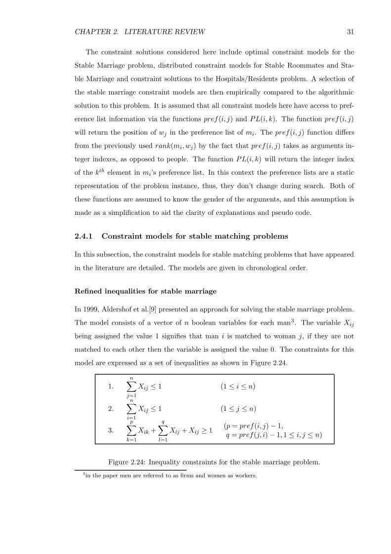
CHAPTER 2. LITERATURE REVIEW 31
The constraint solutions considered here include optimal constraint models for the
Stable Marriage problem, distributed constraint models for Stable Roommates and Sta-
ble Marriage and constraint solutions to the Hospitals/Residents problem. A selection of
the stable marriage constraint models are then empirically compared to the algorithmic
solution to this problem. It is assumed that all constraint models here have access to pref-
erence list information via the functions pref(i, j) and PL(i, k). The function pref(i, j)
will return the position of wj in the preference list of mi. The pref(i, j) function differs
from the previously used rank(mi, wj) by the fact that pref(i, j) takes as arguments in-
teger indexes, as opposed to people. The function PL(i, k) will return the integer index
of the kth element in mi’s preference list. In this context the preference lists are a static
representation of the problem instance, thus, they don’t change during search. Both of
these functions are assumed to know the gender of the arguments, and this assumption is
made as a simplification to aid the clarity of explanations and pseudo code.
2.4.1 Constraint models for stable matching problems
In this subsection, the constraint models for stable matching problems that have appeared
in the literature are detailed. The models are given in chronological order.
Refined inequalities for stable marriage
In 1999, Aldershof et al.[9] presented an approach for solving the stable marriage problem.
The model consists of a vector of n boolean variables for each man3. The variable Xij
being assigned the value 1 signifies that man i is matched to woman j, if they are not
matched to each other then the variable is assigned the value 0. The constraints for this
model are expressed as a set of inequalities as shown in Figure 2.24.
1.
n∑
j=1
Xij ≤ 1 (1 ≤ i ≤ n)
2.
n∑
i=1
Xij ≤ 1 (1 ≤ j ≤ n)
3.
p∑
k=1
Xik +
q∑
l=1
Xlj + Xij ≥ 1(p = pref(i, j) − 1,q = pref(j, i) − 1, 1 ≤ i, j ≤ n)
Figure 2.24: Inequality constraints for the stable marriage problem.
3in the paper men are referred to as firms and women as workers.

CHAPTER 2. LITERATURE REVIEW 32
In Figure 2.24, Constraint 1 states that each man must be matched to at most one
woman. Similarly Constraint 2 states that each woman must be matched to at most one
man. Constraint 3 can be split into three parts. The first summation will equal 1 if man
i is matched to someone he prefers to woman j. The second summation will equal 1 if
woman j is matched to someone she prefers to man i and Xij will equal 1 if man i and
woman j are matched to each other. Therefore, constraint 3 states that either man i and
woman j are matched to each other, or at least one of them will be matched to a preferred
partner. Aldershof et al. describe a specialised algorithm which both refines the constraints
and reduces the variable domains.
• The set of constraints of type 3 are generated for each (i, j) pair such that either
man i is woman j’s most preferred currently available partner or woman j is man
i’s most preferred currently available partner. Note that if Xij is assigned the value
0 then wj is no longer an available partner for mi.
• The full set of constraints of type 3 is then compared to those generated in the
first step. For each (k, l) pair such that its associated constraint is dominated by a
constraint from the first step, the dominated constraint is removed and the variable
Xkl is set to 0. In this context we say that constraint A dominates constraint B
iff the variables involved in constraint A are a subset of the variables involved in
constraint B. If no such (k, l) pair is found, then the algorithm terminates.
• All variables that have been set to 0 are removed from all constraints and the algo-
rithm restarts.
On termination this algorithm will leave the variable domains in an equivalent state
to the GS-lists, such that Xij = 0 iff wj is not in mi’s GS-list. The authors make no time
or space complexity arguments for this algorithm. However, the space complexity will be
dominated by constraint 3. There are at most O(n2) of these constraints each of which will
constrain Θ(n) variables. Therefore, the total space complexity will be O(n3). The time
complexity will be dominated by the second step in the algorithm. A naive analysis shows
that each dominance check will take at most O(n2) time. Each of the Θ(n) constraints
generated in the first step will then have to be checked against each of the O(n2) other
constraints. Therefore, step two will require O(n3) dominance checks and a total of O(n5)
time. In the worst case each iteration of the algorithm could reduce the problem by one

CHAPTER 2. LITERATURE REVIEW 33
pair and thus the algorithm could iterate at most O(n2) times, making the total worst
case complexity for this algorithm O(n7).
However, by maintaining a smart data structure for the constraints, the complexity of
the first run of the second step could be reduced to O(n4). By “repairing” the domination
checks each time rather than restarting, subsequent runs of that step could reduced the
complexity even further such that the first run of that step dominates the time complexity.
Therefore the total run time for this algorithm could be O(n4). The authors do not claim
to be able to find all stable matchings with these algorithms. However, it should be possible
to incorporate this algorithm with a backtracking search to enumerate all solutions. The
authors then go on to discuss an enumeration technique to generate a random stable
matching. They also discuss how this model and algorithm can be extended to solve the
NP-complete extension of HR where couples are allowed to submit joint preference lists.
A constraint programming approach to the stable marriage problem
In 2001, Gent et al.[40] proposed two models to solve the stable marriage problem. The first
was a simple model that represented each man as a single constrained integer variable xi
and each woman by a similar variable yj. All variables have an initial domain of 1 . . . n.
The domain values represent people meaning that variable xi being assigned the value
j would signify that mi was matched to wj . This model has a constraint between each
(man,woman) pair (xi, yj). This constraint takes the form of an explicit set of disallowed
pairs or forbidden tuples. These constraints are detailed in Figure 2.25.
1. Cij = (p, q)|p = PL(i, p′) ∧ q = PL(j, q′) ∧ p′ > pref(i, j) ∧ q′ > pref(j, i))∪ (p, q)|p = j ∧ q 6= i∪ (p, q)|p 6= j ∧ q = i
Figure 2.25: Constraints for the forbidden tuples stable marriage constraint model.
The set of tuples that make up the constraint detailed in Figure 2.25 contains two
distinct types: the unstable tuples (line 1) and the no-bijection tuples (lines 2,3). The
unstable tuples represent an assignment where this couple would rather be matched to
each other than their assigned partners, thus forming a blocking pair. For example, the
set of unstable tuples for the pair (m1, w2) from the SM instance in Figure 2.26 would
be (4, 3), (4, 5), (5, 3), (5, 5). The no-bijection tuples represent an assignment such that
either the man is matched to the woman and the woman is matched to another man or the
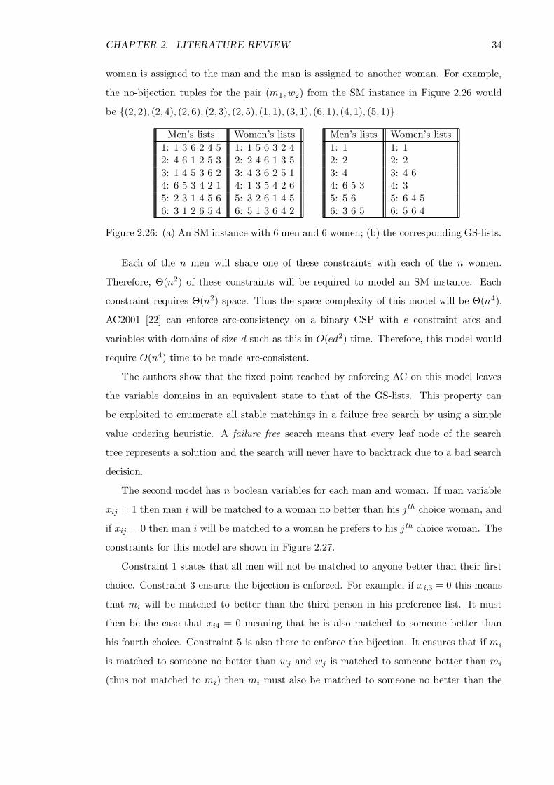
CHAPTER 2. LITERATURE REVIEW 34
woman is assigned to the man and the man is assigned to another woman. For example,
the no-bijection tuples for the pair (m1, w2) from the SM instance in Figure 2.26 would
be (2, 2), (2, 4), (2, 6), (2, 3), (2, 5), (1, 1), (3, 1), (6, 1), (4, 1), (5, 1).
Men’s lists Women’s lists
1: 1 3 6 2 4 5 1: 1 5 6 3 2 42: 4 6 1 2 5 3 2: 2 4 6 1 3 53: 1 4 5 3 6 2 3: 4 3 6 2 5 14: 6 5 3 4 2 1 4: 1 3 5 4 2 65: 2 3 1 4 5 6 5: 3 2 6 1 4 56: 3 1 2 6 5 4 6: 5 1 3 6 4 2
Men’s lists Women’s lists
1: 1 1: 12: 2 2: 23: 4 3: 4 64: 6 5 3 4: 35: 5 6 5: 6 4 56: 3 6 5 6: 5 6 4
Figure 2.26: (a) An SM instance with 6 men and 6 women; (b) the corresponding GS-lists.
Each of the n men will share one of these constraints with each of the n women.
Therefore, Θ(n2) of these constraints will be required to model an SM instance. Each
constraint requires Θ(n2) space. Thus the space complexity of this model will be Θ(n4).
AC2001 [22] can enforce arc-consistency on a binary CSP with e constraint arcs and
variables with domains of size d such as this in O(ed2) time. Therefore, this model would
require O(n4) time to be made arc-consistent.
The authors show that the fixed point reached by enforcing AC on this model leaves
the variable domains in an equivalent state to that of the GS-lists. This property can
be exploited to enumerate all stable matchings in a failure free search by using a simple
value ordering heuristic. A failure free search means that every leaf node of the search
tree represents a solution and the search will never have to backtrack due to a bad search
decision.
The second model has n boolean variables for each man and woman. If man variable
xij = 1 then man i will be matched to a woman no better than his j th choice woman, and
if xij = 0 then man i will be matched to a woman he prefers to his j th choice woman. The
constraints for this model are shown in Figure 2.27.
Constraint 1 states that all men will not be matched to anyone better than their first
choice. Constraint 3 ensures the bijection is enforced. For example, if xi,3 = 0 this means
that mi will be matched to better than the third person in his preference list. It must
then be the case that xi4 = 0 meaning that he is also matched to someone better than
his fourth choice. Constraint 5 is also there to enforce the bijection. It ensures that if mi
is matched to someone no better than wj and wj is matched to someone better than mi
(thus not matched to mi) then mi must also be matched to someone no better than the

CHAPTER 2. LITERATURE REVIEW 35
1. xi1 = 1 (1 ≤ i ≤ n)2. yj1 = 1 (1 ≤ j ≤ n)3. xip = 0 → xip+1 = 0 (1 ≤ i ≤ n, 2 ≤ p ≤ lmi )4. yjq = 0 → yjq+1 = 0 (1 ≤ j ≤ n, 2 ≤ q ≤ lwj )
5. xip = 1 ∧ yjq = 0 → xip+1 = 1 (1 ≤ i, j ≤ n, p = pref(i, j), q = pref(j, i))6. yjq = 1 ∧ xip = 0 → yjq+1 = 1 (1 ≤ i, j ≤ n, p = pref(i, j), q = pref(j, i))7. xip = 1 → yjq+1 = 1 (1 ≤ i, j ≤ n, p = pref(i, j), q = pref(j, i))8. yjq = 1 → xip+1 = 1 (1 ≤ i, j ≤ n, p = pref(i, j), q = pref(j, i))
Figure 2.27: Constraints for the boolean stable marriage constraint model.
next woman after wj in his preference list. Constraint 7 is the stability constraint. If mi
is matched to someone no better than wj then wj must not be matched to anyone worse
than mi. Constraints 2,4,6 and 8 are the female equivalents of 1,3,5 and 7 respectively.
In a non-binary CSP with e constraints, variables with domains of size d and constraints
of arity r, AC can be established in O(edr) time [20]. In this case, we have e = O(n2),
d = 2 and r = 3; therefore, AC can be established in O(n2) time for this model. We
have Θ(n2) variables and Θ(n2) constraints, so the space complexity of this model is also
Θ(n2). The authors show that enforcing AC on this model reduces the variables’ domains
to the equivalent to the bounds of the GS-lists, meaning that enforcing AC on this model is
sufficient to find both the man-optimal and woman-optimal stable matchings. Therefore,
this encoding can be used to find a stable matching in time linear to the size of the
problem input. Thus it is of optimal time complexity. Furthermore, the authors state that
establishing and maintaining the bounds of the GS-lists throughout search is sufficient to
find all stable matchings without failure due to a bad branching decision.
An empirical study of the stable marriage problem with ties and incomplete
lists
In 2002, Gent and Prosser [44] extended the forbidden tuples constraint model proposed
in 2001 [40] to solve the stable marriage problem with ties and incomplete preference
lists (SMTI). The authors present empirical results obtained by using this model to find
the maximum and minimum cardinality stable matchings for randomly generated SMTI
instances. Pseudo-code is given for an instance generator (detailed in appendix B.3) which
generates problem instances for given probabilities for both the volume of ties and the
incompleteness of the preference lists. This was then used to generate instances with a
fixed probability of incompleteness while varying the probability of ties from 0 to 1. This
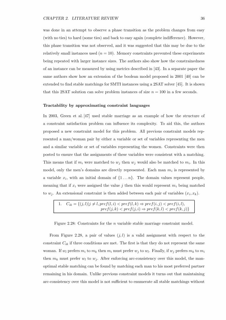
CHAPTER 2. LITERATURE REVIEW 36
was done in an attempt to observe a phase transition as the problem changes from easy
(with no ties) to hard (some ties) and back to easy again (complete indifference). However,
this phase transition was not observed, and it was suggested that this may be due to the
relatively small instances used (n = 10). Memory constraints prevented these experiments
being repeated with larger instance sizes. The authors also show how the constrainedness
of an instance can be measured by using metrics described in [43]. In a separate paper the
same authors show how an extension of the boolean model proposed in 2001 [40] can be
extended to find stable matchings for SMTI instances using a 2SAT solver [45]. It is shown
that this 2SAT solution can solve problem instances of size n = 100 in a few seconds.
Tractability by approximating constraint languages
In 2003, Green et al. [47] used stable marriage as an example of how the structure of
a constraint satisfaction problem can influence its complexity. To aid this, the authors
proposed a new constraint model for this problem. All previous constraint models rep-
resented a man/woman pair by either a variable or set of variables representing the men
and a similar variable or set of variables representing the women. Constraints were then
posted to ensure that the assignments of these variables were consistent with a matching.
This means that if mi were matched to wj then wj would also be matched to mi. In this
model, only the men’s domains are directly represented. Each man mi is represented by
a variable xi, with an initial domain of 1 . . . n. The domain values represent people,
meaning that if xi were assigned the value j then this would represent mi being matched
to wj . An extensional constraint is then added between each pair of variables (xi, xk).
1. Cik = (j, l)|j 6= l, pref(l, i) < pref(l, k) ⇒ pref(i, j) < pref(i, l),pref(j, k) < pref(j, i) ⇒ pref(k, l) < pref(k, j)
Figure 2.28: Constraints for the n variable stable marriage constraint model.
From Figure 2.28, a pair of values (j, l) is a valid assignment with respect to the
constraint Cik if three conditions are met. The first is that they do not represent the same
woman. If wl prefers mi to mk then mi must prefer wj to wl. Finally, if wj prefers mk to mi
then mk must prefer wl to wj. After enforcing arc-consistency over this model, the man-
optimal stable matching can be found by matching each man to his most preferred partner
remaining in his domain. Unlike previous constraint models it turns out that maintaining
arc-consistency over this model is not sufficient to enumerate all stable matchings without

CHAPTER 2. LITERATURE REVIEW 37
backtracking due to an incorrect decision.
This model requires n(n−1)2 such constraints to model the problem, each of which is of
size Θ(n2). This is an overall space complexity of Θ(n4), the same as the forbidden tuples
model proposed in 2001 [40]. However, in practical terms, it requires less than half the
space to store the model which should yield improved performance.
Desk-mates (stable matching) with privacy of preferences, and a new dis-
tributed CSP framework
In a workshop in 2004 and later in a conference in 2005, Silaghi et al. [82, 83] proposed
a distributed constraint model DisWCSP that can be use to solve the stable desk-mates
problem. This problem (more commonly known as the stable roommates problem) is a
generalisation of the stable marriage problem. Here the problem has the added requirement
that the participants’ preference lists must remain private. This paper details a distributed
constraint framework within which this problem can be solved. No complexity argument
is given for this specific problem, but the framework has a worst case time complexity of
O(nn+2). In 2006 a follow up paper was published [10]. In this paper, this solution is
parameterised to allow the level of privacy to be selected at runtime. The levels of privacy
are measured by how much information about other people’s preference lists can be gained
from the messages being passed around as part of the distributed algorithm. It is shown
that higher privacy requirements adversely affect the efficiency of the solution.
Modeling and solving the stable marriage problem using constraint program-
ming
In 2005, Manlove and O’Malley [67] proposed two new constraint models for the Stable
Marriage problem which follow on from those proposed in 2001 [40]. The first model,
referred to as the n+1-valued encoding, has 2n variables each with a domain of 1 . . . n+
1. Here the domain values represent preferences rather than people. This means that
if xi were assigned the value 2, this would represent mi being matched to the second
person on his preference list. A variable being assigned the value n + 1 indicates that the
corresponding person is not matched. This model has Θ(n2) binary constraints, as shown
in Figure 2.29.
Constraints 1 and 2 enforce stability over the model. Considering Constraint 1, if
mi (represented by variable xi) is to be matched to someone no better than woman wj

CHAPTER 2. LITERATURE REVIEW 38
1. xi ≥ p → yj ≤ q (1 ≤ i ≤ n, 1 ≤ p ≤ lmi , j = PL(i, p), q = pref(j, i))2. yj ≥ q → xi ≤ p (1 ≤ j ≤ n, 1 ≤ q ≤ lwj , i = PL(j, q), p = pref(i, j))
3. yj 6= q → xi 6= p (1 ≤ j ≤ n, 1 ≤ q ≤ lwj , i = PL(j, q), p = pref(i, j))
4. xi 6= q → yj 6= p (1 ≤ i ≤ n, 1 ≤ p ≤ lmi , j = PL(i, p), q = pref(j, i))
Figure 2.29: Constraints for the n+1-valued stable marriage constraint model.
(represented by variable yj) then wj must not consider any man worse than mi. Constraint
2 is similar, with the exception that the male and female roles are reversed. Constraints
3 and 4 ensure that the matching is a bijection. Constraint 3 states that if wj is not
matched to mi then mi must not be matched to wj. Constraint 4 is similar, except the
male and female roles are reversed. Constraints 3 and 4 could be combined to form a
single constraint, xi 6= q ↔ yj 6= p. This would reduce the total number of constraints by
twenty-five percent, however the model would still require Θ(n2) constraints.
Enforcing arc-consistency over an implication constraint such as these can be achieved
in O(d) time, where d is the size of the variable’s domain. For example, to propagate
Constraint 1 we would first check if the condition xi ≥ p were true at the head of search,
which can be done in O(1) time. This will then be rechecked each time a value is removed
from the domain of xi. If at any point the condition is found to be true then the second
part of the constraint yj ≤ q will be enforced by removing all values from yj which are
greater than q, and this can be achieved in O(1) time. Due to the fact that this model
contains Θ(n2) constraints and the variable domains are of size n, enforcing arc-consistency
over this model can be achieved in O(n3) time. As with the forbidden tuples constraint
model proposed in 2001 [40], enforcing AC on this model reduces the variable domains to
a state equivalent to the GS-lists produced by the EGS algorithm.
The second proposed model is a follow-on to the boolean encoding given in 2001 [40].
This model has 2n2 variables: n for each man and woman and each has an initial domain of
0, 1, 2, 3. Unlike a traditional constraint model each domain value has a specific meaning.
The value 0 ∈ xij means man mi has not yet proposed to woman wj . This value is removed
when this proposal is made. The value 2 /∈ xij means woman wj would be removed from
man mi’s preference list by the man-oriented EGS algorithm. The value 3 /∈ xij means
woman wj would be removed from man mi’s preference list by the woman-oriented EGS
algorithm. The value 1 is used as a dummy value to ensure that the variable domains
are not reduced to the empty set since this would cause the constraint solver to fail and
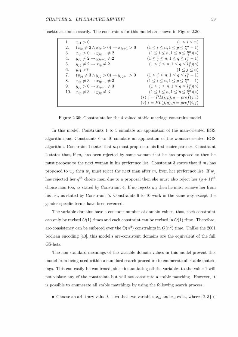
CHAPTER 2. LITERATURE REVIEW 39
backtrack unnecessarily. The constraints for this model are shown in Figure 2.30.
1. xi1 > 0 (1 ≤ i ≤ n)2. (xip 6= 2 ∧ xip > 0) → xip+1 > 0 (1 ≤ i ≤ n, 1 ≤ p ≤ lmi − 1)3. xip > 0 → yjq+1 6= 2 (1 ≤ i ≤ n, 1 ≤ p ≤ lmi )(∗)4. yjq 6= 2 → yjq+1 6= 2 (1 ≤ j ≤ n, 1 ≤ q ≤ lwj − 1)
5. yjq 6= 2 → xip 6= 2 (1 ≤ j ≤ n, 1 ≤ q ≤ lwj )()
6. yj1 > 0 (1 ≤ j ≤ n)7. (yjq 6= 3 ∧ yjq > 0) → yjq+1 > 0 (1 ≤ j ≤ n, 1 ≤ q ≤ lwj − 1)
8. xip 6= 3 → xip+1 6= 3 (1 ≤ i ≤ n, 1 ≤ p ≤ lmi − 1)9. yjq > 0 → xip+1 6= 3 (1 ≤ j ≤ n, 1 ≤ q ≤ lwj )()
10. xip 6= 3 → yjq 6= 3 (1 ≤ i ≤ n, 1 ≤ p ≤ lmi )(∗)(∗) j = PL(i, p), q = pref(j, i)() i = PL(j, q), p = pref(i, j)
Figure 2.30: Constraints for the 4-valued stable marriage constraint model.
In this model, Constraints 1 to 5 simulate an application of the man-oriented EGS
algorithm and Constraints 6 to 10 simulate an application of the woman-oriented EGS
algorithm. Constraint 1 states that mi must propose to his first choice partner. Constraint
2 states that, if mi has been rejected by some woman that he has proposed to then he
must propose to the next woman in his preference list. Constraint 3 states that if mi has
proposed to wj then wj must reject the next man after mi from her preference list. If wj
has rejected her qth choice man due to a proposal then she must also reject her (q + 1)th
choice man too, as stated by Constraint 4. If wj rejects mi then he must remove her from
his list, as stated by Constraint 5. Constraints 6 to 10 work in the same way except the
gender specific terms have been reversed.
The variable domains have a constant number of domain values, thus, each constraint
can only be revised O(1) times and each constraint can be revised in O(1) time. Therefore,
arc-consistency can be enforced over the Θ(n2) constraints in O(n2) time. Unlike the 2001
boolean encoding [40], this model’s arc-consistent domains are the equivalent of the full
GS-lists.
The non-standard meanings of the variable domain values in this model prevent this
model from being used within a standard search procedure to enumerate all stable match-
ings. This can easily be confirmed, since instantiating all the variables to the value 1 will
not violate any of the constraints but will not constitute a stable matching. However, it
is possible to enumerate all stable matchings by using the following search process:
• Choose an arbitrary value i, such that two variables xik and xil exist, where 2, 3 ∈

CHAPTER 2. LITERATURE REVIEW 40
Dik and 2, 3 ∈ Dil (meaning mi has more than one woman remaining in his
domain). If no such man exists then the current variable domains represent a stable
matching.
• In the left branch of the search tree force mi to be matched to his best remaining
choice woman wj . This is done by removing the value 3 from xik+1 where k =
pref(i, j). Re-run the arc-consistency algorithm and choose another man.
• On backtracking remove wj from the domain of mi, by removing the value 2 from
yjl where k = pref(j, i).
Another way to find all stable matchings with this model would be to add a variable
x′i for each mi, along with the channelling constraints given in Figure 2.31. This new set
of variables will then be used as the search variables for the problem. This will allow
the search process total freedom to iterate over these variables using any standard search
strategy.
1. xip 6= 2 → x′i 6= p (1 ≤ i ≤ n, 1 ≤ p ≤ lmi )
2. xip 6= 3 → x′i 6= p (1 ≤ i ≤ n, 1 ≤ p ≤ lmi )
3. x′i = p → xip+1 6= 3 (1 ≤ i ≤ n, 1 ≤ p ≤ lmi )
4. x′i > p → yjq 6= 2 (1 ≤ i ≤ n, 1 ≤ p ≤ lmi , j = PL(i, p), q = pref(j, i))
Figure 2.31: Channelling constraints for the 4-valued stable marriage constraint model.
In Figure 2.31 Constraints 1 and 2 state that if mi’s pth choice partner has been
removed from his domain via either the male or female set of constraints then she will be
removed from the domain of x′i. If mi is assigned his pth choice partner via the x′
i variable,
then Constraint 3 will remove 3 from the domain of xip+1. This will effectively remove all
lesser women from his domain. If mi is rejected by his previous favourite partner yj via
the x′i variable, then Constraint 4 will force yj to be matched to a better partner than mi.
Adding these constraints will not increase either the run time or space complexities of this
model. However, they will increase the space requirements by around twenty-five percent
and will probably increase the run time by a similar amount.
Distributed stable matching problems
In 2005, Brito and Meseguer [25] proposed distributed constraint solutions for both the
Stable Marriage and the Stable Roommates problems. Their solutions for both problems

CHAPTER 2. LITERATURE REVIEW 41
focus on maintaining the privacy of each participant’s preference list. These models ex-
tend the forbidden tuples model proposed by Gent et al. [40]. Each man and woman is
represented by an agent. If two agents share a constraint (i.e. the represented participants
are in each other’s preference lists) then each agent has its own partially complete version
of the constraint. Each agent is only aware of the part of the constraint that can be con-
structed from the preference list of the participant it represents. These constraints are then
propagated via a cut down version of a distributed forward checking algorithm previously
proposed by the same authors [24]. The authors do not give a complexity argument for
their solutions. However, they do give empirical results of some experiments comparing
their model against a distributed version of the EGS algorithm. In 2006, a follow up paper
was published [26] in which the authors show how this solution can be extended to solve
the more general problem with ties and incomplete preference lists.
A constraint programming approach to the Hospitals/Residents problem
In a workshop in 2005 and later in a conference in 2007, Manlove et al.[69, 70] presented
three different approaches to solving the Hospitals/Residents problem within the constraint
environment. For the first solution the authors show how a hospital hj with a capacity
cj > 1 can be “cloned” into cj hospitals each with a capacity of 1. Using this technique
any HR problem instance can be converted into a Stable Marriage instance. This will
make the instance solvable by any stable marriage constraint model. Using this approach
the preference lists in the resulting Stable Marriage instance would be a factor of c larger
than those of the original Hospitals/Residents instance, which implies that this approach
will require significantly more memory in order to find a solution.
The second solution is an extension of the n-valued stable marriage constraint model
proposed in 2005 [67]. This model consists of n variables xi one representing each of the n
residents. Representing each of the m hospitals are c variables yj,1 to yj,c. The domains of
the resident variables represent preferences. This means that if xi were assigned the value
3 this would represent resident i being matched to its third choice hospital. Each resident
variable also initially has the value m + 1 in its domain. Any resident assigned this value
will be unmatched. Similarly the values in the hospitals’ variable domains also represent
preferences in the same way and they have a similar value n + 1 to represent a hospital
post being unassigned. The constraints for this model are given in Figure 2.32.
Constraint 1 eliminates symmetric solutions by enforcing a total order on the posts for

CHAPTER 2. LITERATURE REVIEW 42
1. yjk < yjk+1 (1 ≤ j ≤ m, 1 ≤ k ≤ cj − 1)2. yjk ≥ q → xi ≤ p (1 ≤ j ≤ m, 1 ≤ k ≤ cj , 1 ≤ q ≤ lhj )()
3. xi 6= p → yjk 6= q (1 ≤ i ≤ n, 1 ≤ p ≤ lri , 1 ≤ k ≤ cj)(∗)4. (xi ≥ p ∧ yjk−1 < q) → yjk ≤ q (1 ≤ i ≤ n, 1 ≤ p ≤ lri , 1 ≤ k ≤ cj)(∗)5. yjcj
< q → xi 6= p (1 ≤ j ≤ m, cj ≤ q ≤ lhj )()
() i = PL(j, q), p = pref(i, j)(∗) j = PL(i, p), q = pref(j, i)
Figure 2.32: Constraints for the Hospitals/Residents Problem constraint model.
each hospital, meaning that hospital hj must prefer the resident assigned to post yjk to
the resident assigned to post yjk+1. Constraint 2 states that if one of hospital hj ’s posts
is going to be assigned to a resident no better than resident ri then resident ri must not
be assigned to a hospital worse than hj . If a hospital hj is removed from a resident ri’s
domain then Constraint 3 will remove resident ri from the domain of all the variables
representing hospital hj . If resident ri is to be assigned to a hospital no better than hj
and the hospital’s k − 1th post is going to be assigned to a better resident than ri then
Constraint 4 will ensure that hospital hj ’s kth post is assigned to a resident no worse than
ri. Finally, Constraint 5 states that if hospital hj ’s last post is being assigned to a resident
that is better than ri then hj will be removed from ri’s domain. This constraint model
consists of O(Lc) constraints, where L is the total combined length of the preference lists
and c is the largest capacity of all the hospitals. The variable domains will initially be
of size O(n + m). Each of the constraints in Figure 2.32 can be revised in O(1) time.
Therefore, enforcing arc-consistency over this model can be achieved in O(Lc(n + m))
time.
The third solution is a specialised n-ary constraint written by the author and is given
in detail in Chapter 5. Manlove et al. [69, 70] then go on to demonstrate the versatility
of these constraint solutions by showing how they can be easily extended to solve harder
variants of the problem. These extensions are covered in detail in Chapter 6.
2.4.2 Evaluating the constraint stable marriage solutions
A summary of the theoretical complexities of the stable marriage constraint models re-
viewed in this Section is shown in Table 2.1.
The time complexities of two of the constraint solutions to the Stable Marriage prob-
lem have been proven to equal that of the EGS algorithm (detailed in Figure 2.14). How-
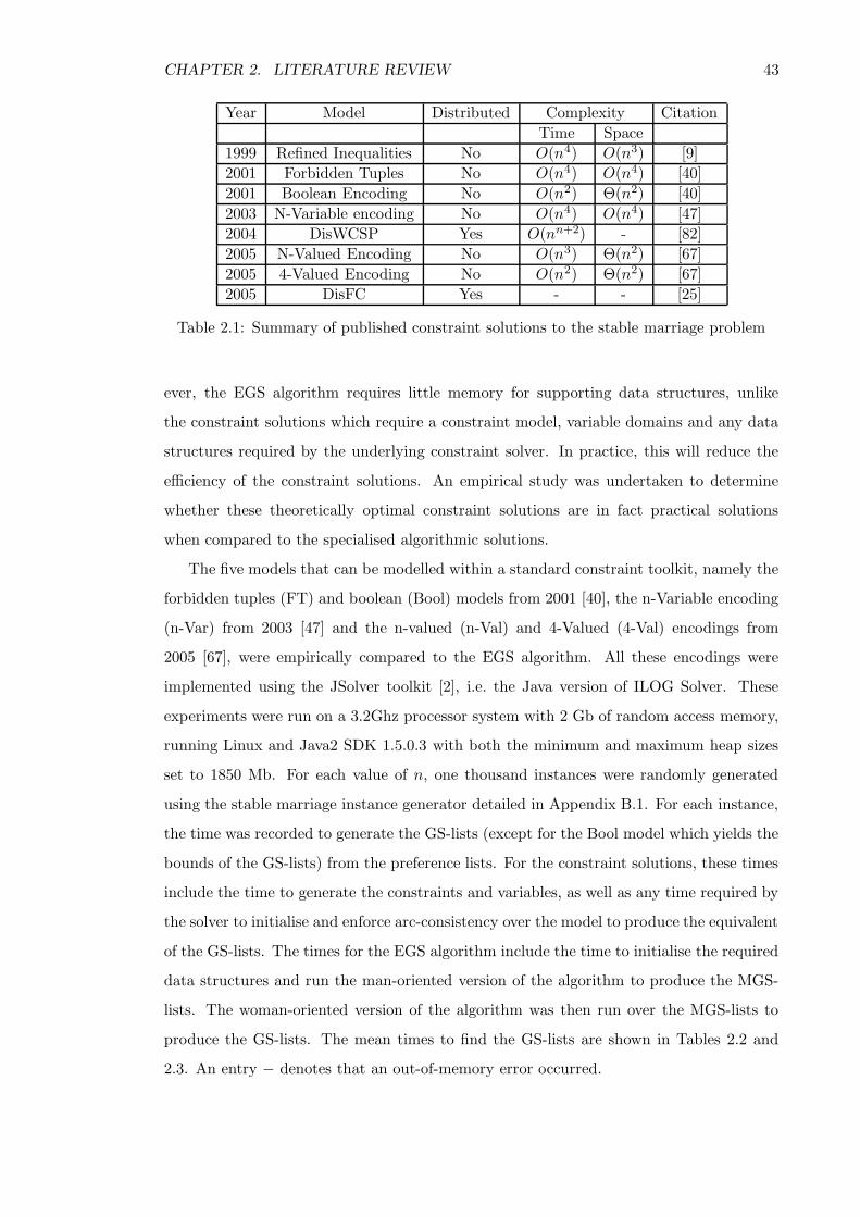
CHAPTER 2. LITERATURE REVIEW 43
Year Model Distributed Complexity Citation
Time Space
1999 Refined Inequalities No O(n4) O(n3) [9]
2001 Forbidden Tuples No O(n4) O(n4) [40]
2001 Boolean Encoding No O(n2) Θ(n2) [40]
2003 N-Variable encoding No O(n4) O(n4) [47]
2004 DisWCSP Yes O(nn+2) - [82]
2005 N-Valued Encoding No O(n3) Θ(n2) [67]
2005 4-Valued Encoding No O(n2) Θ(n2) [67]
2005 DisFC Yes - - [25]
Table 2.1: Summary of published constraint solutions to the stable marriage problem
ever, the EGS algorithm requires little memory for supporting data structures, unlike
the constraint solutions which require a constraint model, variable domains and any data
structures required by the underlying constraint solver. In practice, this will reduce the
efficiency of the constraint solutions. An empirical study was undertaken to determine
whether these theoretically optimal constraint solutions are in fact practical solutions
when compared to the specialised algorithmic solutions.
The five models that can be modelled within a standard constraint toolkit, namely the
forbidden tuples (FT) and boolean (Bool) models from 2001 [40], the n-Variable encoding
(n-Var) from 2003 [47] and the n-valued (n-Val) and 4-Valued (4-Val) encodings from
2005 [67], were empirically compared to the EGS algorithm. All these encodings were
implemented using the JSolver toolkit [2], i.e. the Java version of ILOG Solver. These
experiments were run on a 3.2Ghz processor system with 2 Gb of random access memory,
running Linux and Java2 SDK 1.5.0.3 with both the minimum and maximum heap sizes
set to 1850 Mb. For each value of n, one thousand instances were randomly generated
using the stable marriage instance generator detailed in Appendix B.1. For each instance,
the time was recorded to generate the GS-lists (except for the Bool model which yields the
bounds of the GS-lists) from the preference lists. For the constraint solutions, these times
include the time to generate the constraints and variables, as well as any time required by
the solver to initialise and enforce arc-consistency over the model to produce the equivalent
of the GS-lists. The times for the EGS algorithm include the time to initialise the required
data structures and run the man-oriented version of the algorithm to produce the MGS-
lists. The woman-oriented version of the algorithm was then run over the MGS-lists to
produce the GS-lists. The mean times to find the GS-lists are shown in Tables 2.2 and
2.3. An entry − denotes that an out-of-memory error occurred.
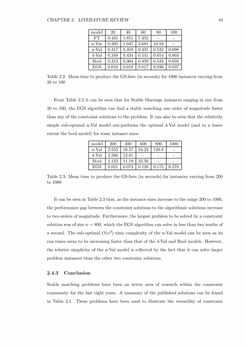
CHAPTER 2. LITERATURE REVIEW 44
model 20 40 60 80 100
FT 0.431 1.851 7.352 - -
n-Var 0.395 1.047 3.681 10.59 -
n-Val 0.317 0.358 0.431 0.532 0.698
4-Val 0.348 0.434 0.541 0.654 0.803
Bool 0.313 0.364 0.450 0.533 0.659
EGS 0.010 0.018 0.017 0.036 0.037
Table 2.2: Mean time to produce the GS-lists (in seconds) for 1000 instances varying from20 to 100
From Table 2.2 it can be seen that for Stable Marriage instances ranging in size from
20 to 100, the EGS algorithm can find a stable matching one order of magnitude faster
than any of the constraint solutions to the problem. It can also be seen that the relatively
simple sub-optimal n-Val model out-performs the optimal 4-Val model (and to a lesser
extent the bool model) for some instance sizes.
model 200 400 600 800 1000
n-Val 2.553 16.57 54.23 128.8 -
4-Val 2.566 12.81 - - -
Bool 2.123 11.18 32.56 - -
EGS 0.021 0.073 0.126 0.175 0.278
Table 2.3: Mean time to produce the GS-lists (in seconds) for instances varying from 200to 1000
It can be seen in Table 2.3 that, as the instance sizes increase to the range 200 to 1000,
the performance gap between the constraint solutions to the algorithmic solutions increase
to two orders of magnitude. Furthermore, the largest problem to be solved by a constraint
solution was of size n = 800, which the EGS algorithm can solve in less than two tenths of
a second. The sub-optimal O(n3) time complexity of the n-Val model can be seen as its
run times seem to be increasing faster than that of the 4-Val and Bool models. However,
the relative simplicity of the n-Val model is reflected by the fact that it can solve larger
problem instances than the other two constraint solutions.
2.4.3 Conclusion
Stable matching problems have been an active area of research within the constraint
community for the last eight years. A summary of the published solutions can be found
in Table 2.1. These problems have been used to illustrate the versatility of constraint
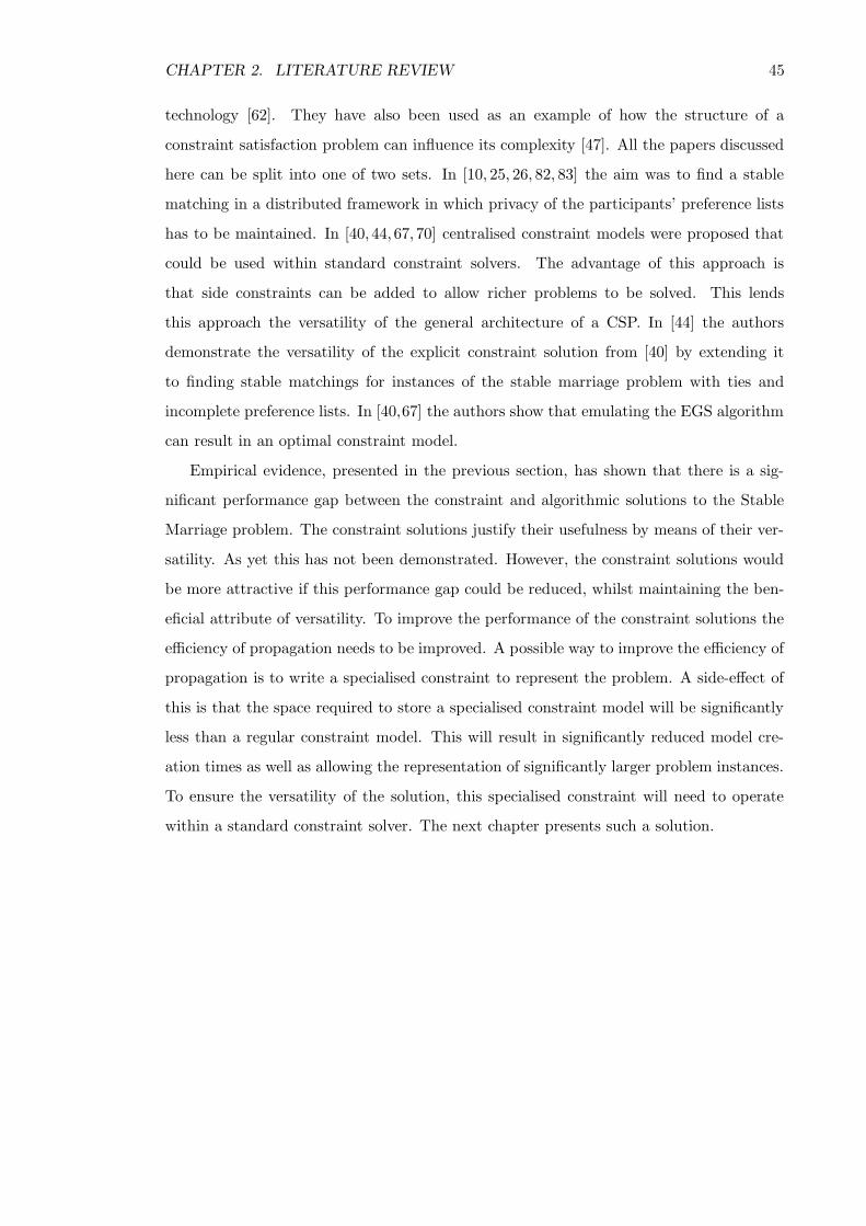
CHAPTER 2. LITERATURE REVIEW 45
technology [62]. They have also been used as an example of how the structure of a
constraint satisfaction problem can influence its complexity [47]. All the papers discussed
here can be split into one of two sets. In [10, 25, 26, 82, 83] the aim was to find a stable
matching in a distributed framework in which privacy of the participants’ preference lists
has to be maintained. In [40, 44, 67, 70] centralised constraint models were proposed that
could be used within standard constraint solvers. The advantage of this approach is
that side constraints can be added to allow richer problems to be solved. This lends
this approach the versatility of the general architecture of a CSP. In [44] the authors
demonstrate the versatility of the explicit constraint solution from [40] by extending it
to finding stable matchings for instances of the stable marriage problem with ties and
incomplete preference lists. In [40,67] the authors show that emulating the EGS algorithm
can result in an optimal constraint model.
Empirical evidence, presented in the previous section, has shown that there is a sig-
nificant performance gap between the constraint and algorithmic solutions to the Stable
Marriage problem. The constraint solutions justify their usefulness by means of their ver-
satility. As yet this has not been demonstrated. However, the constraint solutions would
be more attractive if this performance gap could be reduced, whilst maintaining the ben-
eficial attribute of versatility. To improve the performance of the constraint solutions the
efficiency of propagation needs to be improved. A possible way to improve the efficiency of
propagation is to write a specialised constraint to represent the problem. A side-effect of
this is that the space required to store a specialised constraint model will be significantly
less than a regular constraint model. This will result in significantly reduced model cre-
ation times as well as allowing the representation of significantly larger problem instances.
To ensure the versatility of the solution, this specialised constraint will need to operate
within a standard constraint solver. The next chapter presents such a solution.

Chapter 3
Specialised constraint models for
the Stable Marriage problem
3.1 Introduction
In this chapter, two new specialised constraints for the stable marriage problem are pre-
sented. Initially the constraint will be defined for the classical SM problem with n men,
n women and complete preferences. Later it will be shown how these models can be ex-
tended to allow incomplete preference lists. The first is a binary constraint which acts
over a single (man,woman) pair. O(n2) of these constraints are required to model a stable
marriage instance. The second is an n-ary constraint which can model a problem instance
with a single constraint. When made arc-consistent both of these constraints reduce the
problem to a state equivalent to that of the GS-lists. We prove that arc-consistency can
be enforced over the n-ary constraint in O(n2) time. This means that it can produce the
GS-lists, and thus find a stable matching, in time linear in the size of the preference lists,
which is optimal. Empirical results are then presented, in Section 3.4, which show that
both constraints significantly improve on the performance of previous constraint solutions
to this problem.
3.2 Specialised binary constraint (SM2)
A stable matching can be defined as a bijection of men to women such that no blocking
pair exists. Therefore, an intuitive way to model this problem as a specialised constraint
would be to have a constraint for each man/woman pair which ensures they do not become
46

CHAPTER 3. SM SPECIALISED CONSTRAINT MODELS 47
a blocking pair or violate the bijection.
A specialised binary constraint (SM2) is now presented for the Stable Marriage prob-
lem [94]. This specialised constraint should be considered an object with attributes and
methods which act upon it. We therefore present those attributes and methods.
3.2.1 The constraint model and supporting data structures
A constrained integer variable is associated with each man and each woman, such that,
zi | 1 ≤ i ≤ n corresponds to the set of men and zj | n + 1 ≤ j ≤ 2n to the set
of women. In Stable Marriage instance I, mi is represented by the variable zi and wj
is represented by the variable zn+j . For ease of explanation, the variables may be used
in place of the person they represent. In general, a variable with an index i such as zi,
will represent a man and a variable with a j index will represent a woman. The variable
domains are initialised to 1 . . . n. The domain values represent preferences, such that
variable zk being assigned the value l represents the kth person being married to their lth
choice of partner. The problem is represented in this way to help simplify the propagation
of this constraint. Propagation occurs when it can be proven that a value cannot appear
in any solution. There are two cases in which propagation can occur in this constraint.
The first is if the lower bound of variable zi which represents mi (or wi−n) equals a,
where a = rank(mi, wj) (or a = rank(wi−n,mk)). In this case we must remove from the
domain of zn+j (or zk) the set R of values that represent men (or women) that wj (or
mk) ranks lower than mi (or wi−n). This can be achieved by removing all domain values
greater than rank(wj ,mi) (or rank(mk, wi−n)) from the domain of zn+j (or zk). This
type of propagation can occur either at the head of propagation or when the lower bound
of a variable changes. The second case when propagation occurs is when the value a is
removed from the domain of zi in which case, to ensure the bijection, the value b must be
removed from the domain of zk, where a = rank(mi, wk−n) and b = rank(wk−n,mi) (or
a = rank(wi−n,mk) and b = rank(mk, wi−n)).
Men’s lists Women’s lists
m1: w1 w3 w2 w4 w1: m1 m3 m2 m4
m2: w4 w1 w2 w3 w2: m2 m4 m1 m3
m3: w1 w4 w3 w2 w3: m3 m4 m2 m1
m4: w3 w4 w2 w1 w4: m1 m3 m4 m2
Figure 3.1: A stable marriage instance of size n = 4.
CHAPTER 3. SM SPECIALISED CONSTRAINT MODELS 48
SM2 is a binary constraint which acts over a pair of variables (zi, zj), which represents
the pair (mi, wj−n) in the matching. To model a stable marriage instance, using this
constraint, will require one SM2 constraint for each (man,woman) pair (mi, wj). Therefore,
it requires Θ(n2) of these constraints to model any given stable marriage instance.
The SM2 constraint assumes that it has access to the following functions:
• PL(k, a) where 1 ≤ k ≤ 2n and 1 ≤ a ≤ n, will return the index of the variable
representing the ath person in the preference list of the person represented by the
variable zk. For example, from the instance shown in Figure 3.1, PL(3, 2) will return
8. Because, z8 is the variable that represents w4 and w4 is the 2nd woman in m3’s
preference list. Similarly, PL(8, 2) will return 3.
• pref(k, l) where 1 ≤ k, l ≤ 2n, will return the rank of the person represented by
variable zl in the preference list of the person represented by zk. For example, from
the instance shown in Figure 3.1, pref(3, 8) will return 2, because, z8 is the variable
that represents w4 and w4 is the 2nd woman in m3’s preference list. Similarly,
pref(8, 3) will also return 2. Because, m3 is the 2nd man in w4’s preference list.
• min(dom(x)) will return the smallest value remaining in the domain of variable x.
• setMax(dom(x), k)1 will delete all values from the domain of variable x which are
strictly greater than the value k.
• delV al(dom(x), k) will delete the value k from the domain of variable x.
The min(dom(x)), setMax(dom(x), k) and delV al(dom(x), k) functions are assumed
to be supplied by the underlying constraint solver. This constraint is intended to be
solver independent and thus no assumptions are made about the implementations of these
methods. However, Van Hentenryck et al in Section 4 of their 1992 paper [96] detail an
implementation of an integer domain in which all these functions can run in constant time.
Therefore, for purposes of the complexity argument these functions are assumed to run in
constant time.
Each SM2 constraint has the following attributes:
• x : The local representation of the first constrained variable. For ease of explanation,
we assume that x represents mi.
1Note that this method does not necessarily change the upper bound of dom(x). If the maximum valuein dom(x) is less than k then this method will have no effect.

CHAPTER 3. SM SPECIALISED CONSTRAINT MODELS 49
• y : The local representation of the second constrained variable. For ease of explana-
tion, we assume that x represents wj.
• xPy : The rank of the person represented by variable x in the preference list of the
person represented by variable y.
• yPx : The rank of the person represented by variable y in the preference list of the
person represented by variable x.
The SM2 constraint is designed to operate within an AC5 style framework (Section
2.2). Therefore, to implement this constraint two methods are required, init and remV al.
The init method is called to initiate the propagation. The remV al method is called when
a domain value is removed from the domain of one of the constrained variables. These
methods are detailed below:
1. init()2. if min(dom(x)) ≥ xPy then3. setMax(dom(y),yPx)4. end if5. if min(dom(y)) ≥ yPx then6. setMax(dom(x),xPy)7. end if
Figure 3.2: The init method of the SM2 constraint.
init() The init() method (Figure 3.2) is called to initiate the propagation. This method
checks if mi prefers wj to any other woman in his domain (line 2). If so, then wj must not
consider any partner worse than mi (line 3), otherwise, (mi, wj) may form a blocking pair.
Symmetrically, it also checks if wj prefers mi to any other man in her domain (line 5) and
acts accordingly (line 6). Domain reductions caused by this method are the equivalent of
a proposal in the EGS algorithm (shown in Figure 2.14 in Section 2.4).
remVal(k, a) The remV al(k, a) method (Figure 3.3) is called when the value a has been
removed from the domain of the kth constrained variable. The code as stated assumes that
k = 1, meaning that a value has been removed from the man variable x. If the removed
value a equals mi’s rank for wj (line 2), this means that mi can no longer be matched
to wj . To maintain the bijection, wj ’s rank for mi is removed from wj’s domain (line 3).
This type of domain reduction is the equivalent of a rejection. If mi prefers wj to any

CHAPTER 3. SM SPECIALISED CONSTRAINT MODELS 50
1. remVal(k, a)2. if a = xPy then3. delVal(dom(y),yPx)4. end if5. if min(dom(x)) ≥ xPy then6. setMax(dom(y),yPx)7. end if
Figure 3.3: The remV al method of the SM2 constraint.
other woman in his current domain (line 5), then wj must not consider any man she ranks
lower than mi (line 6). As with the init method, any domain reduction caused by line 5
is the equivalent of a proposal in the EGS algorithm. To complete this constraint we need
to drop the assumption that k = 1. To do this a conditional statement should be added
such that if k = 1, the above code is run. Alternately if k = 2 then similar code is run in
which the x and y terms and the xPy and yPx terms are swapped.
3.2.2 Complexity of SM2
Neither init nor remV al (as shown in Figures 3.2 and 3.3) contains any loops and each
uses only functions that are assumed to run in constant time, so both init and remV al
run in O(1) time. During propagation the init method will be called at most once for each
constraint, and the remV al method will be called at most once for each of the Θ(n) values
in the initial domains of the two constrained variables. Therefore, a single SM2 constraint
will require at most O(n) time during propagation. Θ(n2) SM2 constraints are required
to model a problem instance. Therefore, in the worst case it would take O(n3) time to
enforce arc-consistency over that model. Each SM2 constraint holds two integer variables
to record the preferences and two references to the variables it constrains. Therefore, each
constraint requires O(1) space. As it requires Θ(n2) SM2 constraints to model an instance
of SM, the model would require Θ(n2) space.
3.2.3 Worked example
This section shows how a constraint model using this constraint would propagate the
domains for the Stable Marriage instance shown in Figure 3.4. This is done to demonstrate
the behaviour of the SM2 constraint, to highlight its inherent inefficiencies and provide a
comparison for future more efficient solutions. In this walk-through, the constraints are
referred to as Ci,j (1 ≤ i ≤ n < j ≤ 2n). A Java style attribute selector is used to indicate
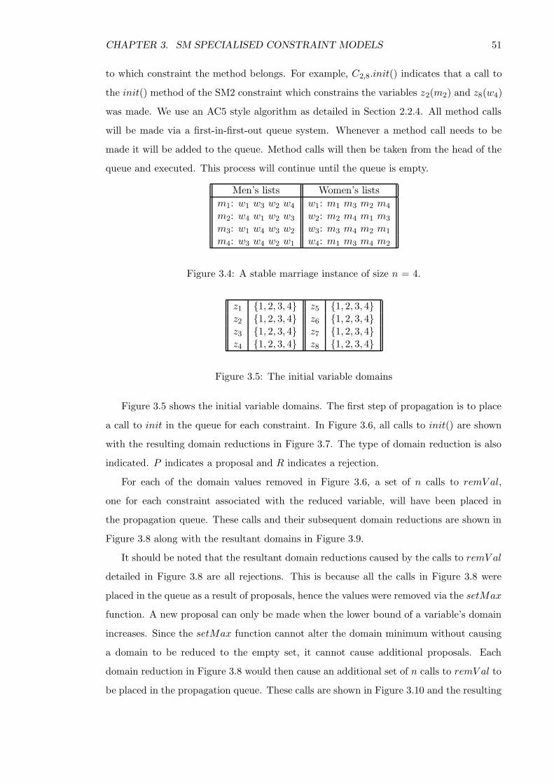
CHAPTER 3. SM SPECIALISED CONSTRAINT MODELS 51
to which constraint the method belongs. For example, C2,8.init() indicates that a call to
the init() method of the SM2 constraint which constrains the variables z2(m2) and z8(w4)
was made. We use an AC5 style algorithm as detailed in Section 2.2.4. All method calls
will be made via a first-in-first-out queue system. Whenever a method call needs to be
made it will be added to the queue. Method calls will then be taken from the head of the
queue and executed. This process will continue until the queue is empty.
Men’s lists Women’s lists
m1: w1 w3 w2 w4 w1: m1 m3 m2 m4
m2: w4 w1 w2 w3 w2: m2 m4 m1 m3
m3: w1 w4 w3 w2 w3: m3 m4 m2 m1
m4: w3 w4 w2 w1 w4: m1 m3 m4 m2
Figure 3.4: A stable marriage instance of size n = 4.
z1 1, 2, 3, 4 z5 1, 2, 3, 4z2 1, 2, 3, 4 z6 1, 2, 3, 4z3 1, 2, 3, 4 z7 1, 2, 3, 4z4 1, 2, 3, 4 z8 1, 2, 3, 4
Figure 3.5: The initial variable domains
Figure 3.5 shows the initial variable domains. The first step of propagation is to place
a call to init in the queue for each constraint. In Figure 3.6, all calls to init() are shown
with the resulting domain reductions in Figure 3.7. The type of domain reduction is also
indicated. P indicates a proposal and R indicates a rejection.
For each of the domain values removed in Figure 3.6, a set of n calls to remV al,
one for each constraint associated with the reduced variable, will have been placed in
the propagation queue. These calls and their subsequent domain reductions are shown in
Figure 3.8 along with the resultant domains in Figure 3.9.
It should be noted that the resultant domain reductions caused by the calls to remV al
detailed in Figure 3.8 are all rejections. This is because all the calls in Figure 3.8 were
placed in the queue as a result of proposals, hence the values were removed via the setMax
function. A new proposal can only be made when the lower bound of a variable’s domain
increases. Since the setMax function cannot alter the domain minimum without causing
a domain to be reduced to the empty set, it cannot cause additional proposals. Each
domain reduction in Figure 3.8 would then cause an additional set of n calls to remV al to
be placed in the propagation queue. These calls are shown in Figure 3.10 and the resulting

CHAPTER 3. SM SPECIALISED CONSTRAINT MODELS 52
method Unsupported values type
1 C1,5.init() (z1,2, 3, 4) P(z5,2, 3, 4) P
2 C1,6.init()
3 C1,7.init()
4 C1,8.init()
5 C2,5.init()
6 C2,6.init() (z2,4) P
7 C2,7.init()
8 C2,8.init()
9 C3,5.init()
10 C3,6.init()
11 C3,7.init() (z3,4) P
12 C3,8.init()
13 C4,5.init()
14 C4,6.init()
15 C4,7.init() (z7,3, 4) P
16 C4,8.init()
Figure 3.6: Calls made to init, where P indicates that the domain reduction was equivalentto a proposal.
z1 1 z5 1z2 1, 2, 3 z6 1, 2, 3, 4z3 1, 2, 3 z7 1, 2z4 1, 2, 3, 4 z8 1, 2, 3, 4
Figure 3.7: The variable domains after the calls to init detailed in Figure 3.6
domains are shown in Figure 3.11.
In Figure 3.10 all domain reductions are proposals. This is because all the calls to
remV al processed in Figure 3.10 were placed in the propagation queue as a result of a
rejection (as shown in Figure 3.8). In a rejection, mi’s preference for wj is removed from
the domain of x as a result of a call to remV al(2, k), where k equals wj’s preference for
mi. Therefore, a rejection could not directly cause another rejection. This is because the
only value that could be removed via a rejection must have already been removed to cause
the initial domain reduction. Each domain reduction in Figure 3.10 would then cause an
additional set of n calls to remV al to be placed in the propagation queue, these calls are
shown in Figure 3.12 along with the resultant domains in Figure 3.13.
As can be seen in Figures 3.8, 3.10 and 3.12, the set of n calls to remV al for each
domain reduction results in at most one further domain reduction. This will always be
the case, assuming there are no additional side constraints. A value v1 being removed

CHAPTER 3. SM SPECIALISED CONSTRAINT MODELS 53
method Unsupported values type1 C1,5.remV al(2, 2)2 C2,5.remV al(2, 2)3 C3,5.remV al(2, 2) (z3,1) R4 C4,5.remV al(2, 2)5 C1,5.remV al(2, 3)6 C2,5.remV al(2, 3) (z2,2) R7 C3,5.remV al(2, 3)8 C4,5.remV al(2, 3)9 C1,5.remV al(2, 4)
10 C2,5.remV al(2, 4)11 C3,5.remV al(2, 4)12 C4,5.remV al(2, 4) (z4,4) R13 C1,5.remV al(1, 2)14 C1,6.remV al(1, 2)15 C1,7.remV al(1, 2)16 C1,8.remV al(1, 2)17 C1,5.remV al(1, 3)18 C1,6.remV al(1, 3) (z6,3) R19 C1,7.remV al(1, 3)20 C1,8.remV al(1, 3)21 C1,5.remV al(1, 4)22 C1,6.remV al(1, 4)23 C1,7.remV al(1, 4)24 C1,8.remV al(1, 4) (z8,1) R25 C2,5.remV al(1, 4)26 C2,6.remV al(1, 4)27 C2,7.remV al(1, 4)28 C2,8.remV al(1, 4)29 C3,5.remV al(1, 4)30 C3,6.remV al(1, 4) (z6,4) R31 C3,7.remV al(1, 4)32 C3,8.remV al(1, 4)33 C1,7.remV al(2, 4)34 C2,7.remV al(2, 4)35 C3,7.remV al(2, 4)36 C4,7.remV al(2, 4)37 C1,7.remV al(2, 3)38 C2,7.remV al(2, 3)39 C3,7.remV al(2, 3)40 C4,7.remV al(2, 3)
Figure 3.8: Calls made to remV al as a result of the domain reductions detailed in Figure3.6, where R indicates that the domain reduction was equivalent to a rejection.
from the domain of zi, as a result of a proposal, can only cause the removal of the value
v2 from zj , where j = PL(i, v1) and v2 = pref(j, i). A value v1 being removed from the
domain of zi, as a result of a rejection, can only cause a reduction in the domain of zj ,
where j = PL(i,min(zi)). No other proposals will have an effect, because any woman zl
that zi prefers to zj will have already rejected him. Therefore, the largest value in her

CHAPTER 3. SM SPECIALISED CONSTRAINT MODELS 54
z1 1 z5 1z2 1, 3 z6 1, 2z3 2, 3 z7 1, 2z4 1, 2, 3 z8 2, 3, 4
Figure 3.9: The variable domains after the calls to remV al detailed in Figure 3.8
method Unsupported values type1 C2,5.remV al(1, 2)2 C2,6.remV al(1, 2)3 C2,7.remV al(1, 2)4 C2,8.remV al(1, 2)5 C3,5.remV al(1, 1)6 C3,6.remV al(1, 1)7 C3,7.remV al(1, 1)8 C3,8.remV al(1, 1) (z8,3, 4) P9 C4,5.remV al(1, 4)
10 C4,6.remV al(1, 4)11 C4,7.remV al(1, 4)12 C4,8.remV al(1, 4)13 C1,6.remV al(2, 3)14 C2,6.remV al(2, 3)15 C3,6.remV al(2, 3)16 C4,6.remV al(2, 3)17 C1,8.remV al(2, 1)18 C2,8.remV al(2, 1)19 C3,8.remV al(2, 1) (z3,3) P20 C4,8.remV al(2, 1)21 C1,6.remV al(2, 4)22 C2,6.remV al(2, 4)23 C3,6.remV al(2, 4)24 C4,6.remV al(2, 4)
Figure 3.10: Calls made to remV al as a result of the domain reductions detailed in Figure3.8
domain will already be less than her preference for zi. In this case, more than one proposal
could occur during the propagation of a single domain reduction. However the number of
effective proposals will be at most one more than the number of domain values removed.
Therefore, each domain reduction can result in up to n − 1 redundant calls. Figure 3.14
shows the calls to remV al resulting from the domain reductions in Figure 3.12 along with
the resultant domains in Figure 3.15.
Figure 3.16 shows the final calls to remV al resulting from the domain reductions in
Figure 3.14. Figure 3.17 shows the variable domains after propagation. Figure 3.18 shows
the unique stable matching the resulting variable domains represent.

CHAPTER 3. SM SPECIALISED CONSTRAINT MODELS 55
z1 1 z5 1z2 1, 3 z6 1, 2z3 2 z7 1, 2z4 1, 2, 3 z8 2
Figure 3.11: The variable domains after the calls to remV al detailed in Figure 3.10
method Unsupported values type1 C1,8.remV al(2, 3)2 C2,8.remV al(2, 3)3 C3,8.remV al(2, 3)4 C4,8.remV al(2, 3) (z4,2) R5 C1,8.remV al(2, 4)6 C2,8.remV al(2, 4) (z2,1) R7 C3,8.remV al(2, 4)8 C4,8.remV al(2, 4)9 C3,5.remV al(1, 3)
10 C3,6.remV al(1, 3)11 C3,7.remV al(1, 3) (z7,1) R12 C3,8.remV al(1, 3)
Figure 3.12: Calls made to remV al as a result of the domain reductions detailed in Figure3.10
z1 1 z5 1z2 3 z6 1, 2z3 2 z7 2z4 1, 3 z8 2
Figure 3.13: The variable domains after the calls to remV al detailed in Figure 3.12
method Unsupported values type1 C4,5.remV al(1, 2)2 C4,6.remV al(1, 2)3 C4,7.remV al(1, 2)4 C4,8.remV al(1, 2)5 C2,5.remV al(1, 1)6 C2,6.remV al(1, 1) (z6,2) P7 C2,7.remV al(1, 1)8 C2,8.remV al(1, 1)9 C1,7.remV al(2, 1)
10 C2,7.remV al(2, 1)11 C3,7.remV al(2, 1)12 C4,7.remV al(2, 1) (z4,3) P
Figure 3.14: Calls made to remV al as a result of the domain reductions detailed in Figure3.12

CHAPTER 3. SM SPECIALISED CONSTRAINT MODELS 56
z1 1 z5 1z2 3 z6 1z3 2 z7 2z4 1 z8 2
Figure 3.15: The variable domains after the calls to remV al detailed in Figure 3.14
method Unsupported values type1 C1,6.remV al(2, 2)2 C2,6.remV al(2, 2)3 C3,6.remV al(2, 2)4 C4,6.remV al(2, 2)5 C4,5.remV al(1, 3)6 C4,6.remV al(1, 3)7 C4,7.remV al(1, 3)8 C4,8.remV al(1, 3)
Figure 3.16: Calls made to remV al as a result of the domain reductions detailed in Figure3.14
z1 1 z5 1z2 3 z6 1z3 2 z7 2z4 1 z8 2
Figure 3.17: The variable domains after the calls to remV al detailed in Figure 3.16
Men’s lists Women’s lists
m1: w1 w1: m1
m2: w2 w2: m2
m3: w4 w3: m4
m4: w3 w4: m3
Figure 3.18: The unique stable matching for the stable marriage instance given in Figure3.4.

CHAPTER 3. SM SPECIALISED CONSTRAINT MODELS 57
3.2.4 The inherent inefficiency of SM2
In Section 3.2.2, it was shown that when using the SM2 constraint to model an instance of
the Stable Marriage problem, it requires suboptimal O(n3) time to enforce arc-consistency
over that model. The inefficiency can be seen in the worked example. Each value removed
from a variable’s domain results in n calls to the remV al method, one for each of the n
constraints associated with the variable in question. Of these n calls, at most two of them
will cause a further domain reduction.
Therefore, to improve on the complexity of this constraint we need to spend no more
than O(1) time per removed domain value. To achieve this, no more than O(1) constraints
can act over each variable. Therefore, there must be a single n-ary constraint constraining
all variables. Such a constraint is now presented.
3.3 Specialised n-ary constraint (SMN)
A specialised n-ary constraint (SMN) for the Stable Marriage problem is now presented
[93]. SMN is designed to improve on the time complexity of the SM2 constraint presented
in Section 3.2. The space complexity is the same as that of the SM2 constraint, but by
reducing the number of constraints from Θ(n2) to one, this constraint solution is signifi-
cantly more space efficient. The SMN constraint will enforce the same level of consistency
as SM2. This means that, unlike most n-ary constraints, SMN will not enforce generalised
arc-consistency. It achieves only arc-consistency, meaning that the propagation achieved
by this constraint is equivalent to that achieved by a clique of binary constraints, which is
described in more detail later in this section. It will be proven that enforcing this level of
consistency will reduce the variable domains to a state equivalent to that of the GS-lists
as produced by the EGS algorithm (as described in Section 2.4). Therefore, enforcing
arc-consistency using this constraint will be sufficient to find a stable matching for a given
stable marriage instance. Furthermore, it will be proven that maintaining arc-consistency
with SMN as part of a standard backtracking search, using a smallest first value ordering
heuristic, is sufficient to enumerate all stable matchings in a failure free manner. SMN
will be shown to run in O(n2) time, which is linear in the size of the preference lists and
therefore optimal. Empirical evidence will also be given that shows that SMN runs sig-
nificantly faster than all previously published constraint models for the Stable Marriage
problem. Furthermore, evidence shows that for large instances the run time of SMN is

CHAPTER 3. SM SPECIALISED CONSTRAINT MODELS 58
within a factor of four of that required by the EGS algorithm.
3.3.1 The constraint: methods and data structures
A constrained integer variable z is associated with each man and each woman as with the
SM2 constraint, such that zi | 1 ≤ i ≤ n corresponds to the set of men and zi | n+1 ≤
i ≤ 2n to the set of women in a given stable marriage instance I. The values in the
domain of a variable correspond to preferences and are in the range 1 to n, such that if
variable zi is assigned the value k this corresponds to the ith man (or (i − n)th woman)
being married to his (or her) kth choice of partner. If this constraint were implemented in
a Java based constraint solver then the constructor to create an SMN constraint may look
like SMN(z,mpl, wpl), where z is an array of constrained integer variables, mpl is a 2
dimensional integer array representing the male preference lists and wpl is a 2 dimensional
integer array representing the female preference lists.
The SMN constraint assumes that it has access to the following functions:
• PL(k, a) where 1 ≤ k ≤ 2n and 1 ≤ a ≤ n, will return the index of the variable
representing the ath person in the preference list of the person represented by the
variable zk.
• pref(k, l) where 1 ≤ k, l ≤ 2n, will return the rank of the person represented by
variable zl in the preference list of the person represented by zk.
• min(dom(x)) will return the smallest value remaining in the domain of variable x.
• setMax(dom(x), k) will delete all values from the domain of variable x which are
strictly greater than the value k.
• delV al(dom(x), k) will delete the value k from the domain of variable x.
SMN is an n-ary stable marriage constraint that acts over 2n variables, which represent
n men and n women, and has the following attributes:
• z is a set of 2n constrained integer variables representing the n men and n women
that are constrained.
• z is a set of 2n reversible integer variables containing the previous lower bounds of
all z variables, where zi will hold the previous lower bound of variable zi. All are
initially set to 0. Reversible means that, on backtracking the values in z are restored.

CHAPTER 3. SM SPECIALISED CONSTRAINT MODELS 59
The two methods required to propagate this constraint init and remV al are now
described, as well as the auxiliary procedure stable. The
1. remVal(i, a)2. j := PL(i, a)3. delVal(dom(zj),pref(j, i))4. if a = zi then5. stable(i)6. end if
Figure 3.19: The remV al method of the SMN constraint.
remVal(i,a) The method detailed in Figure 3.19 is called when the value a has been
removed from the domain of variable zi. This method could be called for 1 ≤ i ≤ 2n,
meaning that the value a was removed from the domain of a variable representing either
a man or woman. However, to simplify the description, it will be assumed that 1 ≤ i ≤ n,
thus, zi will represent a man. When man mi no longer finds his ath choice of person wj−n
acceptable then wj−n should also find mi unacceptable. Consequently, wj−n’s rank for
mi is removed from the domain of zj (lines 2 and 3). These steps, 2 and 3, maintain the
bijection between a man and a woman. Stability is addressed in steps 4 and 5. Line 4
checks to see if the removed value a is equal to the previous lower bound of zi, i.e. zi,
meaning that mi has been rejected by his previous favourite woman. If this is the case,
we must prevent any person that mi prefers to his current lower bound from considering
a partner worse than mi, and this is handled via the stable(i) procedure. In step 3 a
value may be removed from dom(zj) which will eventually result in a call being made to
remV al(j, pref(j, i)). This call will be made under the condition that pref(j, i) ∈ dom(zj)
when the call to remV al(i, a) was made.
1. stable(i)2. for k := zi + 1 to min(dom(zi)) loop3. j := PL(i, k)4. setMax(dom(zj),pref(j, i))5. end loop6. zi := min(dom(zi))
Figure 3.20: The stable function of the SMN constraint.

CHAPTER 3. SM SPECIALISED CONSTRAINT MODELS 60
stable(i) This procedure is called when the lower bound of dom(zi) increases or when
the constraint is initially created. To simplify the description, it will be assumed that
1 ≤ i ≤ n, thus, zi will represent a man. Previously, the lower bound was zi but now it
has increased to min(dom(zi)). Therefore, all people corresponding to preferences in the
range zi + 1 to min(dom(zi)) may no longer consider a match worse than mi, otherwise
a blocking pair may occur. The loop in lines 2 to 5 iterates over the domain values
removed from the lower bound of zi. It finds the person that corresponds to the removed
domain value (line 3) and then prevents that person from considering any potential match
worse than mi (line 4). zi is then updated with the new lower bound of zi (line 6). In
line 4 the call to setMax may remove values from the domain of zj and this in turn
will generate calls to remV al, meaning that remV al and stable are mutually recursive.
Note that if the assumption was made that SMN had exclusive access to the domains of
the z variables then the loop on line 2 would not be necessary. It would be sufficient
to call setMax(dom(zj), pref(j, i)), where j := PL(i,min(dom(zi))). However, such an
assumption was not made. The constraint as written will maintain consistent domains
when arbitrarily domain reduction occurs at any point during propagation. Assuming
that the appropriate calls to remV al are triggered by these domain reductions.
1. init()2. for i := 1 to 2n loop3. stable(i);4. end loop;
Figure 3.21: The init method of the SMN constraint.
init() The init method is called at the head of propagation and is simply a call to stable
for each of the 2n people. In the initial call to stable(i), zi will equal 0. Consequently, man
mi (or woman wi−n) will make a proposal to his (or her) most preferred woman wj−n (or
man mj) (lines 3 and 4 of procedure stable) removing all less preferred partners from the
domain of zj. These domain removals may generate calls to remV al and, thus, as a result
a cascade of propagations may occur. The call to init is equivalent to an application of
the man and woman oriented versions of the EGS algorithm, as proven in Section 3.3.4.

CHAPTER 3. SM SPECIALISED CONSTRAINT MODELS 61
3.3.2 Enhancing the model for incomplete lists
This encoding can be extended to handle incomplete preference lists. For an SMI instance
of size n, the value n+1 is introduced into the domain of each of the z variables. A variable
being assigned the value n+1 indicates that the corresponding person is unmatched. The
method remV al(i, a) will need to be modified as follows: lines 2 and 3 are performed
conditionally if a ≤ n. Similarly, lines 3 and 4 of the stable(i) procedure are performed
conditionally if k ≤ n. Altering the constraint and model in this way will add a potential
O(n) calls to remV al; none of which will cause further propagation. This extension will
not alter the complexity of these methods.
3.3.3 Arc-consistency in the model
The correctness of SMN is now proven by showing that after propagation all remaining
domain values represent the unique maximal set of arc-consistent domain values. A defini-
tion is given for what it means for a domain value to be arc-consistent with respect to the
SMN constraint. It is then proven that all domain values that remain after propagation
will be arc-consistent with respect to this definition and any removed domain values will
be arc-inconsistent.
Definition 1. A constraint model that uses the SMN constraint is arc-consistent iff
∀i ∈ [1 . . . 2n],∀a ∈ dom(zi),
∀k ∈ [1 . . . 2n], i 6= k,∃b ∈ dom(zk),SMN-consistent((zi, a), (zk , b))
Definition 2.
1. SMN-consistent((zi, a),(zk, b)) ⇔
2. (1 ≤ i ≤ n ∧ 1 ≤ k ≤ n ∧ PL(i, a) 6= PL(k, b)) ∨
3. (n < i ≤ 2n ∧ n < k ≤ 2n ∧ PL(i, a) 6= PL(k, b)) ∨
4. (1 ≤ i ≤ n ∧ n < k ≤ 2n ∧
5. ((PL(i, a) = k ∧ PL(k, b) = i) ∨
6. (pref(i, k) > a ∧ PL(k, b) 6= i) ∨
7. (PL(i, a) 6= k ∧ pref(k, i) > b))) ∨
8. (n < i ≤ 2n ∧ 1 ≤ k ≤ n ∧
9. ((PL(i, a) = k ∧ PL(k, b) = i) ∨
10. (pref(i, k) > a ∧ PL(k, b) 6= i) ∨
11. (PL(i, a) 6= k ∧ pref(k, i) > b)))

CHAPTER 3. SM SPECIALISED CONSTRAINT MODELS 62
For a value a in the domain of zi to be arc-consistent with respect to the SMN con-
straint there needs to be at least one supporting value in all other variable domains. A
value b in the domain of zk supports the value a in the domain of zi (line 1) if the simulta-
neous assignments (zi, a) and (zk, b) are consistent and therefore do not violate the SMN
constraint. The definition of a consistent pair of assignments is dependent on the gender
of the people that the variables zi and zk represent. If both are male then the values a
and b must represent different women (line 2), otherwise the bijection will not be main-
tained (similarly if the two variables both represent women (line 3)). If the two variables
represent one of each gender (line 4 or 8) then consistent assignments must respect both
stability and the bijection. In this case, either zi and zk are matched to each other (line
5 or 9), zi prefers their partner to zk (line 6 or 10) or zk prefers their partner to zi (line 7
or 11).
To prove that SMN produces the unique maximal set of arc-consistent domain values,
we need to prove that any value removed does not belong to this set. Therefore, any
domain values removed by SMN must be arc-inconsistent. For a value a in the domain of
zi to be arc-inconsistent there must exist a variable zk that does not contain any supporting
values for a. This is formally stated in Definition 3.
Definition 3. The value a is arc-inconsistent with respect to variable zi if
∃k ∈ [1 . . . 2n],∀b ∈ dom(zk),¬SMN-consistent((zi, a), (zk, b)).
To aid future proofs, first a lemma is presented which states that if dom(zi) has been
reduced to a single value a then dom(zn+j) will also be reduced to a single value b, where
a = rank(mi, wj)2 and b = rank(wj,mi). This means that, if mi has been assigned to
wj then the bijection will be maintained, as wj will also be assigned to mi. To prove this
lemma, the two possible contradictions are disproved; the first where b /∈ dom(zn+j) and
the second where |dom(zn+j)| > 1. This lemma will then be used to prove two theorems.
The first states that any domain value remaining after propagation is arc-consistent. In
this proof, it is assumed that zi is male, and the two possible cases where zk is either male
or female are considered. When considering zk to be male, it is assumed that dom(zk)
has been reduced to a single value rank(mk, wj), where a = rank(mi, wj), and this is
shown to be a contradiction. When considering zk to be female (wj) the three possible
cases are considered; a < rank(mi, wj), a = rank(mi, wj) and a > rank(mi, wj). In each
case, a proof by contradiction is used, which shows that the required value b exists in
2Note that rank(mi, wj) = pref(i, j + n).
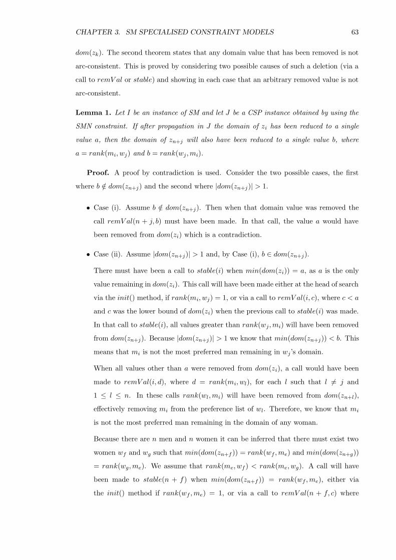
CHAPTER 3. SM SPECIALISED CONSTRAINT MODELS 63
dom(zk). The second theorem states that any domain value that has been removed is not
arc-consistent. This is proved by considering two possible causes of such a deletion (via a
call to remV al or stable) and showing in each case that an arbitrary removed value is not
arc-consistent.
Lemma 1. Let I be an instance of SM and let J be a CSP instance obtained by using the
SMN constraint. If after propagation in J the domain of zi has been reduced to a single
value a, then the domain of zn+j will also have been reduced to a single value b, where
a = rank(mi, wj) and b = rank(wj,mi).
Proof. A proof by contradiction is used. Consider the two possible cases, the first
where b /∈ dom(zn+j) and the second where |dom(zn+j)| > 1.
• Case (i). Assume b /∈ dom(zn+j). Then when that domain value was removed the
call remV al(n + j, b) must have been made. In that call, the value a would have
been removed from dom(zi) which is a contradiction.
• Case (ii). Assume |dom(zn+j)| > 1 and, by Case (i), b ∈ dom(zn+j).
There must have been a call to stable(i) when min(dom(zi)) = a, as a is the only
value remaining in dom(zi). This call will have been made either at the head of search
via the init() method, if rank(mi, wj) = 1, or via a call to remV al(i, c), where c < a
and c was the lower bound of dom(zi) when the previous call to stable(i) was made.
In that call to stable(i), all values greater than rank(wj,mi) will have been removed
from dom(zn+j). Because |dom(zn+j)| > 1 we know that min(dom(zn+j)) < b. This
means that mi is not the most preferred man remaining in wj’s domain.
When all values other than a were removed from dom(zi), a call would have been
made to remV al(i, d), where d = rank(mi, wl), for each l such that l 6= j and
1 ≤ l ≤ n. In these calls rank(wl,mi) will have been removed from dom(zn+l),
effectively removing mi from the preference list of wl. Therefore, we know that mi
is not the most preferred man remaining in the domain of any woman.
Because there are n men and n women it can be inferred that there must exist two
women wf and wg such that min(dom(zn+f )) = rank(wf ,me) and min(dom(zn+g))
= rank(wg,me). We assume that rank(me, wf ) < rank(me, wg). A call will have
been made to stable(n + f) when min(dom(zn+f )) = rank(wf ,me), either via
the init() method if rank(wf ,me) = 1, or via a call to remV al(n + f, c) where

CHAPTER 3. SM SPECIALISED CONSTRAINT MODELS 64
c < rank(wf ,me) and c = zn+f . When this call to stable(n + f) was made, all
values greater than rank(me, wf ) will have been removed from dom(ze), includ-
ing d = rank(me, wg). The resulting call to remV al(e, d) will then have removed
rank(wg,me) from dom(zn+g) which is a contradiction. 2
The following theorem states that all domain values remaining after propagating SMN
are arc-consistent.
Theorem 2. Let I be an instance of SM, and let J be a constraint model of SM instance
I that uses the SMN constraint. Then the domains remaining after propagation in J will
be arc-consistent (as defined in Definition 1).
Proof. We will consider only the case where 1 ≤ i ≤ n, meaning that zi represents mi.
Note that a proof can be obtained for the female variables by swapping the gender specific
terms and adjusting subscripts as appropriate. We assume that a is an arbitrary value
such that a ∈ dom(zi) after propagation in J . We then confirm that a is arc-consistent by
proving the existence of the value b, where b ∈ dom(zk) and k is some arbitrary value in
the range 1 . . . 2n excluding i.
First, consider the case where 1 ≤ k ≤ n, meaning that zk represents mk. In this case
a consistent assignment means mi and mk are not matched to the same woman. In SMN
this means that PL(i, a) 6= PL(k, b) where zi and zk have been assigned the values a and
b respectively. Therefore, b must not equal rank(mk, wj) where a = rank(mi, wj).
A proof by contradiction is used. Assume b = rank(mk, wj) where n + j = PL(i, a),
b ∈ dom(zk) and |dom(zk)| = 1. From Lemma 1 we know that c is the only value in
dom(zn+j), where c = rank(wj,mk). Therefore, the value d, where d = rank(wj,mi),
must have been removed from dom(zn+j) which would have caused a call to be made to
remV al(n+j, d). In that call rank(mi, wj) would have been removed from dom(zi), which
is a contradiction.
Now consider the case where n < k ≤ 2n meaning that zk represents wk−n. For
simplicity we will now refer to wk−n as wj . In this case, a consistent assignment means that
if a = rank(mi, wj) then b = rank(wj ,mi) or if a > rank(mi, wj) then b < rank(wj,mi)
otherwise if a < rank(mi, wj) then b 6= rank(wj,mi). A proof by contradiction is now
used for each case individually.
• a = rank(mi, wj). Assume b = rank(wj ,mi) and b /∈ dom(zk). When b was removed
from dom(zk) a call would have been made to remV al(k, b). In that call, the value

CHAPTER 3. SM SPECIALISED CONSTRAINT MODELS 65
rank(mi, wj) will have been removed from dom(zi) which is a contradiction.
• a > rank(mi, wj). Assume min(dom(zk)) = rank(wj,mi). A call to stable(k) will
have been made while min(dom(zk)) = rank(wj,mi) either via the init() method, if
1 = rank(wj,mi), or via a call to remV al(k, b), where b < rank(wj,mi) and b = zk.
When this call to stable(k) was made all values greater than rank(mi, wj) would
have been removed from dom(zi), including a, which is a contradiction.
• a < rank(mi, wj). Assume b = rank(wj,mi), b ∈ dom(zk) and |dom(zk)| = 1.
From Lemma 1 we know that dom(zi) must contain only rank(mi, wj), which is a
contradiction. 2
Theorem 3 below states that all values removed during the propagation of SMN are
arc-inconsistent.
Theorem 3. Let I be an instance of SM and let J be a constraint model of SM instance
I that uses the SMN constraint. If SMN removes some value v from dom(zi) then that
value is arc-inconsistent as defined in Definition 3.
Proof. We will consider only the case where 1 ≤ i ≤ n meaning that zi represents
mi. A proof can be obtained for the female variables by swapping the gender terms and
adjusting subscripts as appropriate.
The two possible causes of v being removed from dom(zi), line 3 of remV al or line 4
of stable, are considered.
For v to be removed via a call to remV al(n + j, a), then a must have been removed
from dom(n + j), where v = rank(mi, wj) and a = rank(wj,mi). In this call, v would
have been removed from dom(zi). If v were not removed and the assignment zi = v was
made then this would mean that mi was matched to wj but wj was not matched to mi,
which is arc-inconsistent.
For v to be removed via a call to stable(n + j), then min(dom(zn+j)) ≥ rank(wj,mi)
and v > rank(mi, wj). Therefore, we know wj would rather be matched to mi than any
man remaining in her domain. If the assignment zi = v were made then (mi, wj) would
be a blocking pair and therefore arc-inconsistent. 2
Theorem 4. Let I be an instance of SM and let J be a constraint model of SM instance I
that uses the SMN constraint. After propagation in J the resultant variable domains will
represent the unique maximal set of arc-consistent domain values.
CHAPTER 3. SM SPECIALISED CONSTRAINT MODELS 66
Proof. This follows from Theorems 2 and 3. From Theorem 2, it is known that all
remaining domain values after propagating SMN are arc-consistent. From Theorem 3, it
is known that all domain values that are removed as a result of propagating SMN are
arc-inconsistent. This then implies that after propagating SMN the remaining domain
values represent the unique maximal set of arc-consistent domain values. 2
3.3.4 Properties of SMN
As previously stated, unlike most n-ary constraints, SMN enforces only arc-consistency.
The reason for this is that, in 2001, Gent et al.[40] proved that enforcing arc-consistency
over a constraint representation of a stable marriage problem was sufficient to produce
the equivalent of the GS-lists, and therefore to find a stable matching. Furthermore, they
proved that, under certain conditions, all stable matchings can be enumerated without
having to backtrack due to an incorrect decision (i.e. failure-free enumeration). In this
section, it is proven that SMN has the same properties as the model proposed by Gent et
al.
To prove this it is first shown that the resultant variable domains after propagating
SMN are equivalent to the GS-lists. A generalised proof is then given which shows that
the GS-lists of an SMI instance can be split into two distinct sets of lists such that all
stable matchings contained in the original SMI instance exist in one of these two new sets
of list. Both of these sets of lists will contain at least one solution. A further proof then
goes on to state that using the standard branching technique of choosing an arbitrary
variable with a domain size greater than one and instantiating it to the smallest value in
that domain for the left branch, then removing that value for the right branch, will result
in the variable domains being equivalent to the two sets of lists. Therefore, branching in
this way will result in at least one solution at each branch of the search tree.
It is now shown that, given a constraint model J consisting of SMN which models a
given SMI instance I, the domains of the variables in J , following propagation, correspond
to the GS-lists of I, where wj ∈ GS(mi) indicates that wj is in the GS-list of mi. That
is, we prove that, ∀i, j ∈ [1 . . . n], wj ∈ GS(mi) ⇔ rank(mi, wj) ∈ dom(zi), and similarly
∀j, i ∈ [1 . . . n],mi ∈ GS(wj) ⇔ rank(wj,mi) ∈ dom(zn+j). The proof is presented using
two lemmas. The first lemma shows that the arc-consistent domains are equivalent to
subsets of the GS-lists. This is done by proving that the deletions made by the EGS
algorithm applied to I are correspondingly made during propagation in J . The second

CHAPTER 3. SM SPECIALISED CONSTRAINT MODELS 67
lemma shows that the GS-lists of I correspond to a subset of the domains remaining after
propagation in J . This is done by proving that no values in the GS-lists for I could be
removed by SMN3. Note that lmi denotes the length of mi’s preference list, and lwj the
length of wj ’s list.
Lemma 5. For any given i (1 ≤ i ≤ n), let p be an integer (1 ≤ p ≤ lmi ) such that
p ∈ dom(zi) after propagating SMN. Then woman wj, where p = rank(mi, wj), belongs to
the GS-list of mi. An equivalent result holds for the women.
Proof. The GS-lists are constructed as a result of the deletions made by the EGS
algorithm applied to I. We show that the corresponding deletions are made to the relevant
variables’ domains during propagation of SMN. In the following proof, only deletions made
by the man-oriented EGS algorithm are considered. A similar argument can be used to
prove the result for an execution of the woman oriented EGS algorithm.
We prove the following fact by induction on the number of proposals k during an
execution E of the EGS algorithm. If proposal k consists of mi proposing to wj , where
p = rank(mi, wj) and q = rank(wj ,mi), then min(dom(zi)) ≥ p, max(dom(zn+j)) ≤ q
and for each mt such that s = rank(wj,mt) and (q < s ≤ lwj ), r /∈ dom(zt), where
r = rank(mt, wj).
First, consider the base case where k = 1. It must be the case that p = 1, since 1 =
min(dom(zi)). The procedure call stable(i), made by the init() method, will remove all val-
ues greater than q from dom(zn+j), where q = rank(wj,mi), making max(dom(zn+j)) ≤ q.
These domain reductions will in turn cause calls to remV al(n + j, s) to be placed in the
propagation queue for each s such that (q < s ≤ lwj ). In each call to remV al(n + j, s), r
will be removed from dom(zt), where s = rank(wj,mt) and r = rank(mt, wj).
Now consider k = c > 1, we assume that the result holds for k < c. We consider the
cases where p = 1 and p > 1.
• Case (i). For p = 1 the proof is similar to that of the base case.
• Case (ii). Suppose that p > 1. Let wl be any woman such that r = rank(mi, wl) and
r < p. wl must have been deleted from mi’s list by the man-oriented EGS algorithm.
Next, assume s1 = rank(wl,mi). Then mi was deleted from wl’s preference list
3These proofs are adaptations of proofs given for Lemmas 1 and 2 in Section 3 of [40]. Both proofsstart by showing how the EGS algorithm removes a value and then how each of the respective constraintsolutions also removes the equivalent values from the appropriate domains. The proofs given here differ inthe section detailing how the equivalent values are removed as a result of the constraint model.

CHAPTER 3. SM SPECIALISED CONSTRAINT MODELS 68
because she received a proposal from a man mv whom she prefers to mi, where
s2 = rank(wl,mv) and s2 < s1. Since mv proposed to wl before the cth proposal,
we know max(dom(zn+l)) ≤ s2, therefore, s1 /∈ dom(zn+l) and r /∈ dom(zi). The
argument made for wl can be made for any woman whom mi prefers to wj, hence
r /∈ dom(zi) for 1 ≤ r < p, therefore, min(dom(zi)) ≥ p. Before min(dom(zi))
became greater than or equal to r, there must have been a value s ∈ dom(zi) such
that s < r and prior to its removal s = min(dom(zi)). When s was removed, a call
to remV al(i, s) was made. In that call to remV al(i, s), the stable(i) procedure will
have been called. The rest of the proof is then similar to that of the base case. 2
Lemma 6. For each i (1 ≤ i ≤ n), define a domain of values domGS(zi) which is
a subset of the initial values in dom(zi) before propagation as follows: domGS(zi) =
rank(mi, wj) : wj ∈ GS(mi). The domain of each zn+j (1 ≤ j ≤ n) is defined anal-
ogously. Enforcing arc-consistency over SMN could not cause an arbitrary value v to be
removed from some variable’s domain dom(zk) if v ∈ domGS(zk).
Proof. A proof by contradiction is used. Assume that the value v, (where v ∈
domGS(zk)) is the first such value to be removed, by enforcing arc-consistency over SMN,
from dom(zk). Therefore, prior to the removal of v, all values in domGS(zk) exist in
dom(zk). Furthermore, it is assumed that prior to the removal of v, domGS(zk) = dom(zk)
(from Lemma 5).
A domain reduction in SMN can only occur via a call to remV al(i, a) or via a call to
stable(i). These two cases are now considered.
First, consider the case where v was removed from dom(zk) via a call to stable(i). Only
the zi variables are considered, where (1 ≤ i ≤ n), however, a similar proof can be made
for the zj variables (n+1 < j ≤ 2n). A call to stable(i) will remove all values greater than
q, where q = rank(wj ,mi), from dom(zn+l) for each l such that (1 ≤ s ≤ min(dom(zi)))
and s = rank(mi, wl). Therefore, max(dom(zn+l)) ≤ q. For stable(i) to remove the value
v from dom(zk), it must be the case that n < k ≤ 2n, rank(mi, wk−n) ≤ min(domGS(zi))
and v > rank(wk−n,mi). If rank(mi, wk−n) ≤ min(domGS(zi)) it must be the case that
max(domGS(zk)) ≤ rank(wk−n,mi), otherwise (mi, wk−n) would form a blocking pair in
any potential matching. Therefore, v /∈ domGS(zk) which, is a contradiction.
Now consider the case where v was removed from dom(zk) via a call to remV al(i, a).
The call remV al(i, a) must have been made when a was removed from dom(zi). From
our previous assumption, we know that a /∈ domGS(zi). If a /∈ domGS(zi) then v /∈
CHAPTER 3. SM SPECIALISED CONSTRAINT MODELS 69
domGS(zk), where a = rank(mi, wk−n) and v = rank(wk−n,mi), which is a contradiction.
2
The two lemmas above lead to the following theorem.
Theorem 7. Let I be an instance of SM and let J be a CSP instance obtained by the
SMN constraint. Then the domains remaining after propagation in J correspond to the
GS-lists of I in the following sense: for any i, j(1 ≤ i, j ≤ n), wj ∈ GS(mi) if and
only if p ∈ dom(zi), and similarly mi ∈ GS(wj) if and only if q ∈ dom(zn+j), where
rank(mi, wj) = p and rank(wj,mi) = q.
A lemma is now given that will later be used to help prove that SMN can find all
stable matchings without failure as a result of a bad search decision. This lemma states
that, given the GS-lists of an SMI instance I, two new SMI instances I ′1 and I ′2 can be
created. This is done by selecting some man mi that has more than one woman remaining
in his preference list. The SMI instance I ′1 is the same as the instance described by the
GS-lists except that all but mi’s favourite woman have been removed from his preference
list, and him from their preference lists. I ′2 is the same except that mi’s favourite woman
has been removed from his preference list and he has been removed from her list, and the
rest remain. This Lemma states that all stable matchings in I can be found in either I ′1
or I ′2 with no repeats4. In this lemma the term PL(mi) is used to reference the preference
list of mi.
Lemma 8. Let I be an instance of SMI and let I ′ be an SMI instance derived from the
GS-lists of I. If in I ′ there exists some mi who has more than one entry in his preference
list, two SMI instances I ′1 and I ′2 can be derived, where I ′1 is the same as I ′ except that
PL(mi) contains only mi’s first choice woman wj, and I ′2 is the same as I ′ except that wj
has been removed from PL(mi). These instances will then have the following properties:
(i) Any matchings that are stable in I ′1 or I ′2 will also be stable in I.
(ii) I ′1 and I ′2 share no common matchings.
(iii) All stable matchings in I are stable in either I ′1 or I ′2.
4The proof for this lemma is an adaptation of Theorem 5 in Section 2.1 of [68]. The original proofshowed that a constraint encoding could find all stable matchings without failure as a result of a baddecision. In this adaptation the proof is generalized by removing all references to the constraint encoding.

CHAPTER 3. SM SPECIALISED CONSTRAINT MODELS 70
Proof. (i) By standard properties of the GS-lists, any stable matching in I ′ is also
stable in I.
First, consider instance I ′1. We verify that any stable matching M in I ′1 is stable in
I ′. Suppose that the pair (m,w) blocks the matching M in I ′. If w ∈ PL(m) in I ′1, then
(m,w) blocks the matching M in I ′1, so (m,w) must have been deleted from I ′. Hence,
(m,w) = (mi, wl) for some wl such that rank(mi, wl) > rank(mi,mj). Now suppose that
M ′ denotes the man-optimal stable matching in I. Then (mi, wj) ∈ M ′ and it may be
verified that M ′ is also stable in I ′1. Since the same set of men and women are matched
in all stable matchings in I ′1 [37], mi is matched in M . In particular, (mi, wj) ∈ M as wj
is the only woman in mi’s list in I ′1. Hence, (m,w) = (mi, wl) cannot block M in I ′ after
all, as mi prefers wj to wl. Thus M is stable in I.
Next consider I ′2. we verify that any stable matching M in I ′2 is stable in I ′. Suppose
that (m,w) blocks M in I ′. If (m,w) 6= (mi, wj) then (m,w) blocks M in I ′2 so we assume
(m,w) = (mi, wj). In I ′, both mi and wj must have lists of length greater than one (by
the qualifying condition). Therefore, wj is matched in the man-pessimal stable matching
for instance I, which is stable in I ′2. Since the same set of men and women are matched in
all stable matchings in I ′2 [37], wj is matched in M . In particular, wj prefers her partner
in M to mi, so that (mi, wj) cannot block M in I ′. Thus, M is stable in I ′ and hence by
the induction hypothesis M is also stable in I.
(ii) In all stable matchings in I ′1, mi will be matched to wj (as above). Because in I ′2
wj /∈ PL(mi) it follows that I ′1 and I ′2 share no common matchings.
(iii) We now show that any stable matching M1 in I ′, such that (mi, wj) ∈ M1, will
also be a stable matching in I ′1 and any stable matching M2 in I ′, such that (mi, wj) /∈ M2,
will also be a stable matching in I ′2.
First consider instance I ′1. For M1 to be a stable matching in I ′ but not in I ′1, either
some pair (mk, wl) ∈ M1 was removed from I ′1 or a blocking pair exists in I ′1 which
does not exist in I ′. The only pairs to be removed from I ′1 involve mi and, as we know
(mi, wj) ∈ M1, none of the removed pairs could be in M1. As no pairs were added to I ′1,
so no blocking pairs could have been introduced.
Now consider I ′2. For M2 to be a stable matching in I ′ but not in I ′2, either some pair
(mk, wl) ∈ M2 was removed from I ′2 or a blocking pair exists in I ′2 which does not exist in
I ′. The only pair to be removed from I ′2 is (mi,mj) and, it is known that (mi, wj) /∈ M2,
so none of the removed pairs could be in M2. No pairs were added to I ′2, and therefore,
CHAPTER 3. SM SPECIALISED CONSTRAINT MODELS 71
no blocking pairs could have been introduced. 2
Theorem 9. Let I be an instance of SMI and let J be a CSP instance obtained using the
SMN constraint. Then the following search process enumerates all solutions in I without
repetition and without ever failing due to an inconsistency:
• the init() method is called as a preprocessing step. Values removed as a result of this
call will cause a call to the remV al(i, a) method.
• if all domains are arc-consistent and some variable zi has two or more values in its
domain, then the search proceeds by setting zi to the minimum value p in its domain.
Each domain value removed as a result of this instantiation will result in a call to
the remV al(i, a) method which will re-establish arc-consistency. On backtracking,
the value p is removed from the domain of zi. This action will result in the call
remV al(i, p) which will re-establish arc-consistency.
• when a solution is found it is reported and backtracking is forced.
Proof. From Theorem 7 we know that a call to the init() method will reduce the
variable domains to the equivalent of the GS-lists of I. By setting zi to the minimum
value p in its domain, an independent subproblem will be produced which is equivalent
to I ′1 from Lemma 8. On backtracking, removing the value p from the domain of zi will
produce an independent subproblem which is equivalent to I ′2 from Lemma 8. As both I ′1
and I ′2 contain all solutions in I without repetition and as they both contain at least one
stable matching, this decision can never cause a failure. 2
The technique detailed here to enumerate all stable matchings will not match the
optimal worst case time complexity of the algorithm proposed by Gusfield [48], which
can enumerate all stable matchings for a given stable marriage instance in O(m + kn)
time, where m is the sum of the lengths of the preference lists, k is the number of stable
matchings in the instance and n is the number of participants. However, this specialised
constraint solution is significantly easier to implement. Furthermore, empirical analysis
(shown later in Figure 3.42) suggests that the average case time complexity for finding
all solutions with the specialised constraint model matches the worst case complexity of
Gusfield’s algorithm.

CHAPTER 3. SM SPECIALISED CONSTRAINT MODELS 72
3.3.5 Complexity of the model
AC can be enforced using this constraint in O(n2) time which, because the preference
lists are of size O(n2), is optimal for this problem [49]. Each of the two methods and one
auxiliary procedure are examined individually, it is stated how often each can be called
and the complexity of each call.
The init() method is only called once, at the head of search. It contains a single for
loop that cycles 2n times and each iteration makes a call to the stable(i) procedure. Due
to this call to stable(i) being made at the head of search zi will equal min(dom(zi)).
Therefore, the loop in stable(i) (lines 2 to 5) will cycle only once and the time complexity
of each call to stable(i) will be O(1) (because at this point zi = min(dom(zi))). These calls
to stable(i) may cause domain reductions which will in turn cause calls to remV al(i, a).
The remV al(i, a) method can be called at most once for each potential combination of
i and a. remV al(i, a) contains no loops. Thus, with the exception of the possible call to
the stable(i) procedure, which will be addressed below, remV al(i, a) runs in O(1) time5.
There are O(n) potential values for i and O(n) potential values for a. Thus, the total time
complexity for all possible calls to remV al will be O(n2).
The stable(i) procedure is called via the remV al(i, a) method when the lower bound of
dom(zi) changes, or via the init() method at the head of search. The run time complexity
of stable(i) is dependent on the difference between the previous lower bound zi and the
new lower bound of dom(zi). If the lower bound of dom(zi) has increased by k then the
while loop in stable(i) will cycle k+1 times, thus stable(i) will run in O(k) time. However,
the total time complexity of all calls to stable(i) for a fixed value of i is bounded by the
length of the preference list of zi, i.e.O(n). There are O(n) potential values for i. Hence,
the total time complexity for all possible calls to stable will be O(n2). Therefore, the total
time complexity of the single call to init() (which will result in the variable domains being
arc-consistent) will be O(n2).
3.3.6 Worked example
This section presents an example of how a constraint model using the SMN constraint
would propagate the domains for the stable marriage instance shown in Figure 3.22 (which
is the same instance as given in Figure 3.4). In this walk-through, the constraint is referred
5Van Hentenryck et al in Section 4 of their 1992 paper [96] detail an implementation of an integerdomain in which all the functions used here run in constant time.

CHAPTER 3. SM SPECIALISED CONSTRAINT MODELS 73
to as C and a Java style attribute selector is used to indicate which of the constraint’s
methods or functions is being run. An AC5 style environment, as detailed in Chapter 2.2,
is used.
Men’s lists Women’s lists
m1: w1 w3 w2 w4 w1: m1 m3 m2 m4
m2: w4 w1 w2 w3 w2: m2 m4 m1 m3
m3: w1 w4 w3 w2 w3: m3 m4 m2 m1
m4: w3 w4 w2 w1 w4: m1 m3 m4 m2
Figure 3.22: A stable marriage instance of size n = 4.
z1 1, 2, 3, 4 z5 1, 2, 3, 4z2 1, 2, 3, 4 z6 1, 2, 3, 4z3 1, 2, 3, 4 z7 1, 2, 3, 4z4 1, 2, 3, 4 z8 1, 2, 3, 4
Figure 3.23: The initial variable domains
Figure 3.23 shows the initial variable domains. The first step of propagation is to place
a call to init() in the queue. This will in turn make a call to stable for each participant. In
Figure 3.24, the call to init() and the subsequent calls to stable are shown along with the
resulting domain reductions. The type of domain reduction is also indicated. As before,
P indicates a proposal and R indicated a rejection.
method Unsupported values type
1 C.init()
2 C.stable(1) (z5,2, 3, 4) P
3 C.stable(2)
4 C.stable(3)
5 C.stable(4) (z7,3, 4) P
6 C.stable(5) (z1,2, 3, 4) P
7 C.stable(6) (z2,4) P
8 C.stable(7) (z3,4) P
9 C.stable(8)
Figure 3.24: Calls made to the auxiliary procedure stable, called from the init() methodat the head of propagation.
Figure 3.26 shows the set of calls to remV al resulting from the domain reductions in
3.24. Figure 3.8 shows that for the SM2 constraint the same set of domain reductions
caused forty calls to remV al of which only six caused further domain reductions. In

CHAPTER 3. SM SPECIALISED CONSTRAINT MODELS 74
z1 1 z5 1z2 1, 2, 3 z6 1, 2, 3, 4z3 1, 2, 3 z7 1, 2z4 1, 2, 3, 4 z8 1, 2, 3, 4
Figure 3.25: The variable domains after the calls to stable detailed in Figure 3.24
method Unsupported values type1 C.remV al(5, 2) (z3,1) R2 C.remV al(5, 3) (z2,2) R3 C.remV al(5, 4) (z4,4) R4 C.remV al(7, 3)5 C.remV al(7, 4)6 C.remV al(1, 2)7 C.remV al(1, 3) (z6,3) R8 C.remV al(1, 4) (z8,1) R9 C.remV al(2, 4)
10 C.remV al(3, 4) (z6,4) R
Figure 3.26: Calls made to remV al as a result of the domain reductions detailed in Figure3.24
Figure 3.26 it can be seen that with SMN only ten calls to remV al were made, which is
a reduction of the number of redundant calls by thirty.
Figure 3.34 shows the final calls to remV al resulting from the domain reductions in
Figure 3.32. Figure 3.35 shows the variable domains after propagation and Figure 3.36
shows the unique stable matching the resulting variable domains represent.
z1 1 z5 1z2 1, 3 z6 1, 2z3 2, 3 z7 1, 2z4 1, 2, 3 z8 2, 3, 4
Figure 3.27: The variable domains after the calls to remV al() detailed in Figure 3.26
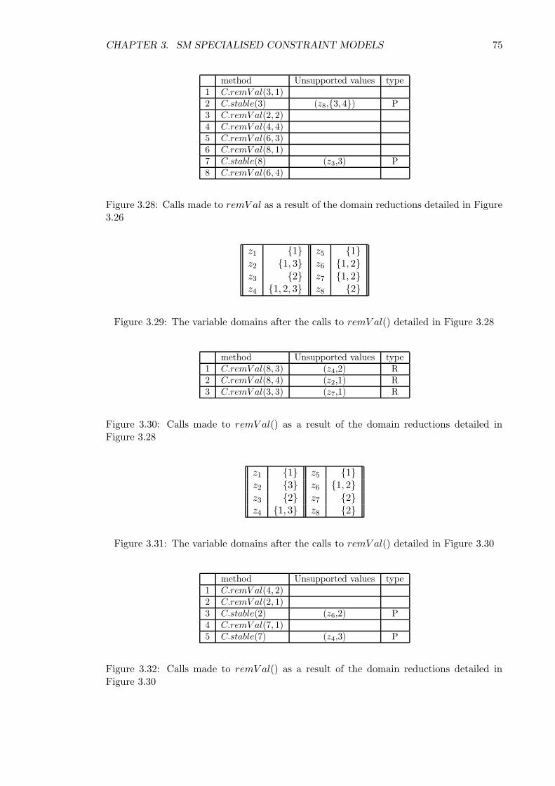
CHAPTER 3. SM SPECIALISED CONSTRAINT MODELS 75
method Unsupported values type1 C.remV al(3, 1)2 C.stable(3) (z8,3, 4) P3 C.remV al(2, 2)4 C.remV al(4, 4)5 C.remV al(6, 3)6 C.remV al(8, 1)7 C.stable(8) (z3,3) P8 C.remV al(6, 4)
Figure 3.28: Calls made to remV al as a result of the domain reductions detailed in Figure3.26
z1 1 z5 1z2 1, 3 z6 1, 2z3 2 z7 1, 2z4 1, 2, 3 z8 2
Figure 3.29: The variable domains after the calls to remV al() detailed in Figure 3.28
method Unsupported values type1 C.remV al(8, 3) (z4,2) R2 C.remV al(8, 4) (z2,1) R3 C.remV al(3, 3) (z7,1) R
Figure 3.30: Calls made to remV al() as a result of the domain reductions detailed inFigure 3.28
z1 1 z5 1z2 3 z6 1, 2z3 2 z7 2z4 1, 3 z8 2
Figure 3.31: The variable domains after the calls to remV al() detailed in Figure 3.30
method Unsupported values type1 C.remV al(4, 2)2 C.remV al(2, 1)3 C.stable(2) (z6,2) P4 C.remV al(7, 1)5 C.stable(7) (z4,3) P
Figure 3.32: Calls made to remV al() as a result of the domain reductions detailed inFigure 3.30
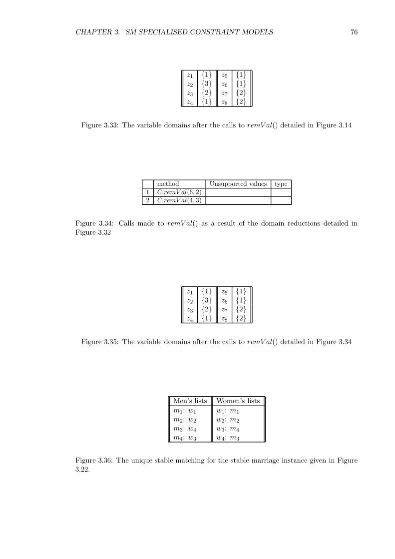
CHAPTER 3. SM SPECIALISED CONSTRAINT MODELS 76
z1 1 z5 1z2 3 z6 1z3 2 z7 2z4 1 z8 2
Figure 3.33: The variable domains after the calls to remV al() detailed in Figure 3.14
method Unsupported values type1 C.remV al(6, 2)2 C.remV al(4, 3)
Figure 3.34: Calls made to remV al() as a result of the domain reductions detailed inFigure 3.32
z1 1 z5 1z2 3 z6 1z3 2 z7 2z4 1 z8 2
Figure 3.35: The variable domains after the calls to remV al() detailed in Figure 3.34
Men’s lists Women’s lists
m1: w1 w1: m1
m2: w2 w2: m2
m3: w4 w3: m4
m4: w3 w4: m3
Figure 3.36: The unique stable matching for the stable marriage instance given in Figure3.22.

CHAPTER 3. SM SPECIALISED CONSTRAINT MODELS 77
3.4 Computational experience
A major part of the thesis statement is that a specialised constraint solution can sig-
nificantly outperform standard toolkit solutions. This section presents experiments that
were run to empirically compare the performance of the specialised constraints detailed in
Sections 3.2 and 3.3 with the toolbox constraint solutions detailed in Section 2.4. The con-
straint solutions compared were: forbidden tuples (FT) and boolean (Bool) models from
2001 [40], the n-Variable encoding (n-Var) from 2003 [47], and the n-valued (n-Val) and
4-Valued (4-Val) Encodings from 2005 [67]. A summary of the time and space complexities
of these models is shown in Table 3.1.
model FT Bool n-Var n-Val 4-Val SM2 SMN
Time O(n4) O(n2) O(n4) O(n3) O(n2) O(n3) O(n2)
Space O(n4) Θ(n2) O(n4) Θ(n2) Θ(n2) Θ(n2) Θ(n2)
Table 3.1: Summary of time and space complexities
All these encodings were implemented using the JSolver toolkit [2], i.e. the Java version
of ILOG Solver. In total these experiments took in excess of 110 CPU hours to run on
a 3.2Ghz processor system with 2 Gb of random access memory, running Linux and Java
SDK 1.5.0.3 with an increased heap size of 1850 Mb.
To ensure a consistent set of data for use in the experiments, three sets of stable mar-
riage instances were randomly generated by the random stable marriage instance generator
detailed in Appendix B.1. Each set of problem instances was generated with complete pref-
erence lists and stored on a hard disc, and the same instances were used for each model.
The instance and sample sizes for each set are given in Table 3.2.
n increment size sample size
10 . . . 100 10 1000
100 . . . 1000 100 1000
1000 . . . 8000 1000 20
Table 3.2: Data Set Sizes
The results obtained from these experiments are now presented in the following cate-
gories: the time taken to generate the constraint models (Section 3.4.1), the time taken
to enforce arc-consistency on the constraint model (Section 3.4.2) and the time taken to
find all stable matchings for the given instance (Section 3.4.3).

CHAPTER 3. SM SPECIALISED CONSTRAINT MODELS 78
3.4.1 Model creation time
Before solving a problem, a constraint solver tool kit must first create a representation
of the problem. This data structure is referred to as a constraint model. Included in the
model creation time is both the time to construct the constraints and variables along with
any time required by the underlying solver to initialise its internal data structures. More
elaborate constraint models can take a significant time to construct, and therefore, have
a negative effect on the overall solution time of the problem. For this reason, the time
to construct the constraint model for each problem instance was measured and recorded.
These times will also include the time used by the solver to initialise its own data structures
required to perform search as well as the actual constraint model. The range of times
recorded for a given model and instance size was very small. Therefore, only the mean
model creation times are displayed. This small range is due to the fact that the model
creation time is affected only by the size of the problem and not its difficulty. All reported
times exclude the time taken to read the problem instance from the disk. The EGS
algorithm has no significant model or data structures to initialise so it has not been included
in these results. Note that the entry ’-’ indicates that an out-of-memory error occurred.
model 20 40 60 80 100
FT 0.319 1.573 6.734 - -
Bool 0.257 0.271 0.305 0.316 0.334
n-Var 0.299 0.842 3.230 9.701 -
n-Val 0.308 0.333 0.354 0.381 0.431
4-Val 0.259 0.275 0.326 0.343 0.359
SM2 0.235 0.244 0.233 0.233 0.236
SMN 0.238 0.234 0.226 0.225 0.224
Table 3.3: Mean model creation time (in seconds) for 1000 instances varying in size from20 to 100
Table 3.3 shows that the FT model with its sub-optimal space complexity of O(n4)
severely limits the size of problems that it can solve, relative to the other models. Despite
having the same O(n4) space complexity as the FT model, the more compact n-Var can
model slightly larger problems.
In Table 3.4 it can be seen that the specialised constraint models can be constructed sig-
nificantly faster and can model significantly larger instances than the toolbox constraint
models. There are two possible explanations for this outcome, the first being that the
toolbox constraint models use significantly more constraints. Bool uses 2n + 6n2 con-
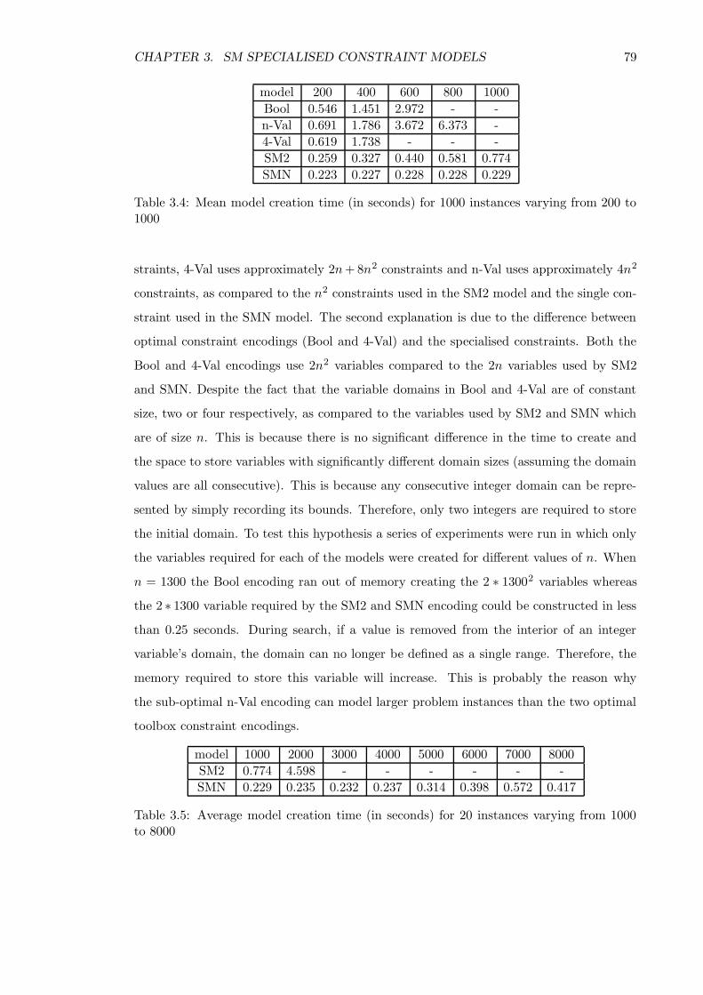
CHAPTER 3. SM SPECIALISED CONSTRAINT MODELS 79
model 200 400 600 800 1000
Bool 0.546 1.451 2.972 - -
n-Val 0.691 1.786 3.672 6.373 -
4-Val 0.619 1.738 - - -
SM2 0.259 0.327 0.440 0.581 0.774
SMN 0.223 0.227 0.228 0.228 0.229
Table 3.4: Mean model creation time (in seconds) for 1000 instances varying from 200 to1000
straints, 4-Val uses approximately 2n + 8n2 constraints and n-Val uses approximately 4n2
constraints, as compared to the n2 constraints used in the SM2 model and the single con-
straint used in the SMN model. The second explanation is due to the difference between
optimal constraint encodings (Bool and 4-Val) and the specialised constraints. Both the
Bool and 4-Val encodings use 2n2 variables compared to the 2n variables used by SM2
and SMN. Despite the fact that the variable domains in Bool and 4-Val are of constant
size, two or four respectively, as compared to the variables used by SM2 and SMN which
are of size n. This is because there is no significant difference in the time to create and
the space to store variables with significantly different domain sizes (assuming the domain
values are all consecutive). This is because any consecutive integer domain can be repre-
sented by simply recording its bounds. Therefore, only two integers are required to store
the initial domain. To test this hypothesis a series of experiments were run in which only
the variables required for each of the models were created for different values of n. When
n = 1300 the Bool encoding ran out of memory creating the 2 ∗ 13002 variables whereas
the 2 ∗ 1300 variable required by the SM2 and SMN encoding could be constructed in less
than 0.25 seconds. During search, if a value is removed from the interior of an integer
variable’s domain, the domain can no longer be defined as a single range. Therefore, the
memory required to store this variable will increase. This is probably the reason why
the sub-optimal n-Val encoding can model larger problem instances than the two optimal
toolbox constraint encodings.
model 1000 2000 3000 4000 5000 6000 7000 8000
SM2 0.774 4.598 - - - - - -
SMN 0.229 0.235 0.232 0.237 0.314 0.398 0.572 0.417
Table 3.5: Average model creation time (in seconds) for 20 instances varying from 1000to 8000
CHAPTER 3. SM SPECIALISED CONSTRAINT MODELS 80
Table 3.5 shows that the relatively large number of constraints required by the SM2
model restricts the instance size it can solve, whereas, the SMN model can model consid-
erably larger instance sizes without difficulty. Note also the anomaly where n = 7000; the
time required to create the SMN model is greater than that when n = 8000. This is likely
a result of the small sample size of twenty for the problem instances in the range 2000 to
8000. A larger sample size would probably see this anomaly disappear. We also see in
Tables 3.3, 3.4 and 3.5 that the SMN model creation time only varies by 0.014 for instance
sizes ranging from 20 to 4000. This is probably due to the fact that the model includes
only one constraint. The only significant change as n increases, for the SMN model, is
the number of variables required. The time to generate the SMN model for instance sizes
ranging from 20 to 4000 is so small, it is assumed that generating this number of variables
is insignificant when compared to the time overhead required by the underlying solver to
initiate its internal data structures. This overhead is estimated to be around 0.2 seconds.
3.4.2 Enforcing arc-consistency
All constraint models included in this study share the property that enforcing
arc-consistency is sufficient to find a solution. For this reason, the time to enforce arc-
consistency over a pre-constructed constraint model was measured and recorded. The
range of times recorded for a given model and instance size was significant. Therefore, the
minimum, maximum and mean values are given for each data set. Note that the entry ’-’
indicates that an out-of-memory error occurred.
From Table 3.6, it can be seen that enforcing arc-consistency over a pre-constructed
constraint model can be achieved in under half a second for all instances where n ≤ 100.
This shows that the time to find a solution for instances of this size is dominated by the
time to create the initial constraint model. For the SMN constraint and to a lesser extent
the SM2 constraint, it can be seen that, as n increases, the maximum time taken to enforce
arc-consistency over a model actually decreases. This could be an indication that a sample
size of 1000 was sufficient to find a problem instance, out of the n!2n possible instances
generated by the instance generator, which was close to the worst case for the smaller
instance sizes. However, for the larger instances, the sample size was insufficient to find an
instance that was sufficiently close to the worst case. It may be the case that the harder
instances are rarer for the larger instances.
In Table 3.7, it appears that, for instances in the range 200 ≤ n ≤ 1000, the difference
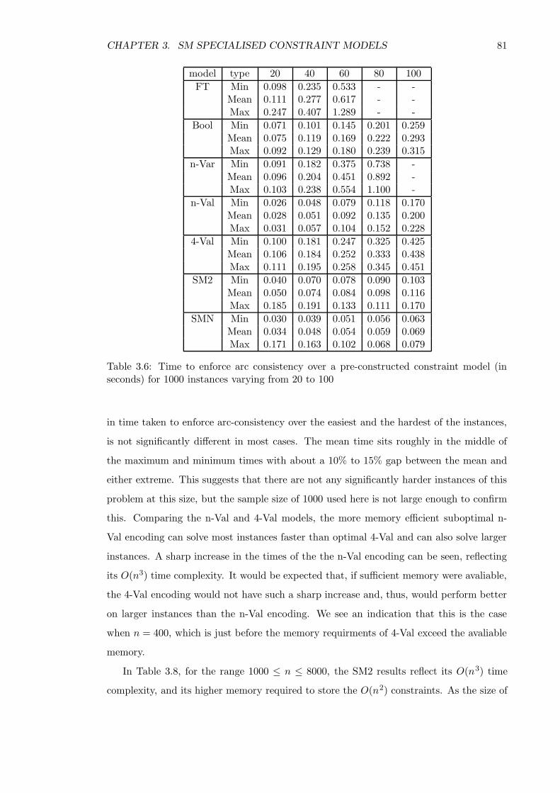
CHAPTER 3. SM SPECIALISED CONSTRAINT MODELS 81
model type 20 40 60 80 100
FT Min 0.098 0.235 0.533 - -Mean 0.111 0.277 0.617 - -Max 0.247 0.407 1.289 - -
Bool Min 0.071 0.101 0.145 0.201 0.259Mean 0.075 0.119 0.169 0.222 0.293Max 0.092 0.129 0.180 0.239 0.315
n-Var Min 0.091 0.182 0.375 0.738 -Mean 0.096 0.204 0.451 0.892 -Max 0.103 0.238 0.554 1.100 -
n-Val Min 0.026 0.048 0.079 0.118 0.170Mean 0.028 0.051 0.092 0.135 0.200Max 0.031 0.057 0.104 0.152 0.228
4-Val Min 0.100 0.181 0.247 0.325 0.425Mean 0.106 0.184 0.252 0.333 0.438Max 0.111 0.195 0.258 0.345 0.451
SM2 Min 0.040 0.070 0.078 0.090 0.103Mean 0.050 0.074 0.084 0.098 0.116Max 0.185 0.191 0.133 0.111 0.170
SMN Min 0.030 0.039 0.051 0.056 0.063Mean 0.034 0.048 0.054 0.059 0.069Max 0.171 0.163 0.102 0.068 0.079
Table 3.6: Time to enforce arc consistency over a pre-constructed constraint model (inseconds) for 1000 instances varying from 20 to 100
in time taken to enforce arc-consistency over the easiest and the hardest of the instances,
is not significantly different in most cases. The mean time sits roughly in the middle of
the maximum and minimum times with about a 10% to 15% gap between the mean and
either extreme. This suggests that there are not any significantly harder instances of this
problem at this size, but the sample size of 1000 used here is not large enough to confirm
this. Comparing the n-Val and 4-Val models, the more memory efficient suboptimal n-
Val encoding can solve most instances faster than optimal 4-Val and can also solve larger
instances. A sharp increase in the times of the the n-Val encoding can be seen, reflecting
its O(n3) time complexity. It would be expected that, if sufficient memory were avaliable,
the 4-Val encoding would not have such a sharp increase and, thus, would perform better
on larger instances than the n-Val encoding. We see an indication that this is the case
when n = 400, which is just before the memory requirments of 4-Val exceed the avaliable
memory.
In Table 3.8, for the range 1000 ≤ n ≤ 8000, the SM2 results reflect its O(n3) time
complexity, and its higher memory required to store the O(n2) constraints. As the size of
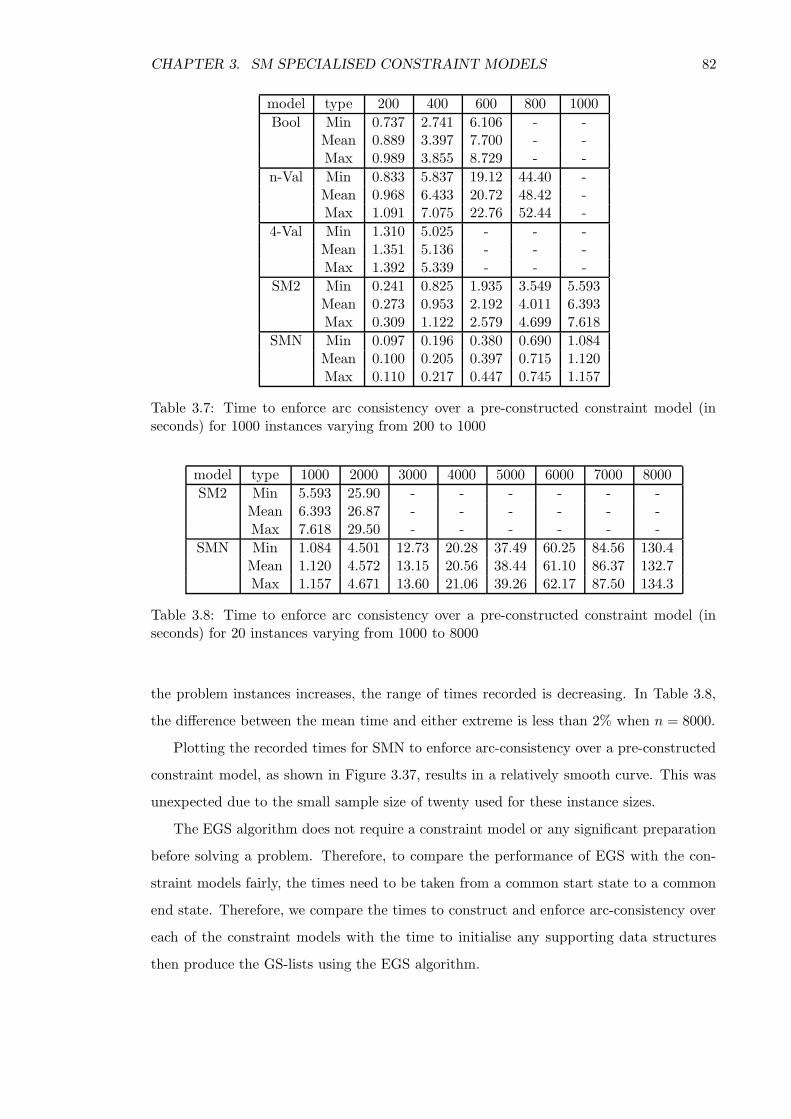
CHAPTER 3. SM SPECIALISED CONSTRAINT MODELS 82
model type 200 400 600 800 1000
Bool Min 0.737 2.741 6.106 - -Mean 0.889 3.397 7.700 - -Max 0.989 3.855 8.729 - -
n-Val Min 0.833 5.837 19.12 44.40 -Mean 0.968 6.433 20.72 48.42 -Max 1.091 7.075 22.76 52.44 -
4-Val Min 1.310 5.025 - - -Mean 1.351 5.136 - - -Max 1.392 5.339 - - -
SM2 Min 0.241 0.825 1.935 3.549 5.593Mean 0.273 0.953 2.192 4.011 6.393Max 0.309 1.122 2.579 4.699 7.618
SMN Min 0.097 0.196 0.380 0.690 1.084Mean 0.100 0.205 0.397 0.715 1.120Max 0.110 0.217 0.447 0.745 1.157
Table 3.7: Time to enforce arc consistency over a pre-constructed constraint model (inseconds) for 1000 instances varying from 200 to 1000
model type 1000 2000 3000 4000 5000 6000 7000 8000
SM2 Min 5.593 25.90 - - - - - -Mean 6.393 26.87 - - - - - -Max 7.618 29.50 - - - - - -
SMN Min 1.084 4.501 12.73 20.28 37.49 60.25 84.56 130.4Mean 1.120 4.572 13.15 20.56 38.44 61.10 86.37 132.7Max 1.157 4.671 13.60 21.06 39.26 62.17 87.50 134.3
Table 3.8: Time to enforce arc consistency over a pre-constructed constraint model (inseconds) for 20 instances varying from 1000 to 8000
the problem instances increases, the range of times recorded is decreasing. In Table 3.8,
the difference between the mean time and either extreme is less than 2% when n = 8000.
Plotting the recorded times for SMN to enforce arc-consistency over a pre-constructed
constraint model, as shown in Figure 3.37, results in a relatively smooth curve. This was
unexpected due to the small sample size of twenty used for these instance sizes.
The EGS algorithm does not require a constraint model or any significant preparation
before solving a problem. Therefore, to compare the performance of EGS with the con-
straint models fairly, the times need to be taken from a common start state to a common
end state. Therefore, we compare the times to construct and enforce arc-consistency over
each of the constraint models with the time to initialise any supporting data structures
then produce the GS-lists using the EGS algorithm.
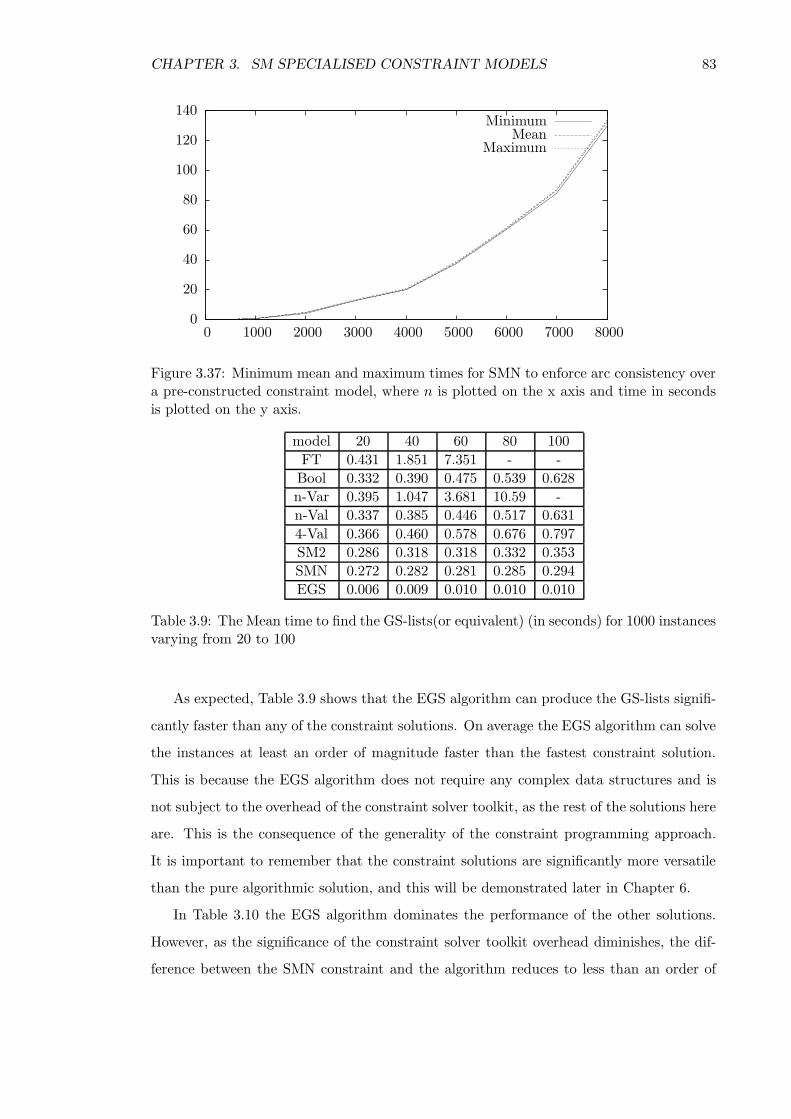
CHAPTER 3. SM SPECIALISED CONSTRAINT MODELS 83
MaximumMean
Minimum
800070006000500040003000200010000
140
120
100
80
60
40
20
0
Figure 3.37: Minimum mean and maximum times for SMN to enforce arc consistency overa pre-constructed constraint model, where n is plotted on the x axis and time in secondsis plotted on the y axis.
model 20 40 60 80 100
FT 0.431 1.851 7.351 - -
Bool 0.332 0.390 0.475 0.539 0.628
n-Var 0.395 1.047 3.681 10.59 -
n-Val 0.337 0.385 0.446 0.517 0.631
4-Val 0.366 0.460 0.578 0.676 0.797
SM2 0.286 0.318 0.318 0.332 0.353
SMN 0.272 0.282 0.281 0.285 0.294
EGS 0.006 0.009 0.010 0.010 0.010
Table 3.9: The Mean time to find the GS-lists(or equivalent) (in seconds) for 1000 instancesvarying from 20 to 100
As expected, Table 3.9 shows that the EGS algorithm can produce the GS-lists signifi-
cantly faster than any of the constraint solutions. On average the EGS algorithm can solve
the instances at least an order of magnitude faster than the fastest constraint solution.
This is because the EGS algorithm does not require any complex data structures and is
not subject to the overhead of the constraint solver toolkit, as the rest of the solutions here
are. This is the consequence of the generality of the constraint programming approach.
It is important to remember that the constraint solutions are significantly more versatile
than the pure algorithmic solution, and this will be demonstrated later in Chapter 6.
In Table 3.10 the EGS algorithm dominates the performance of the other solutions.
However, as the significance of the constraint solver toolkit overhead diminishes, the dif-
ference between the SMN constraint and the algorithm reduces to less than an order of
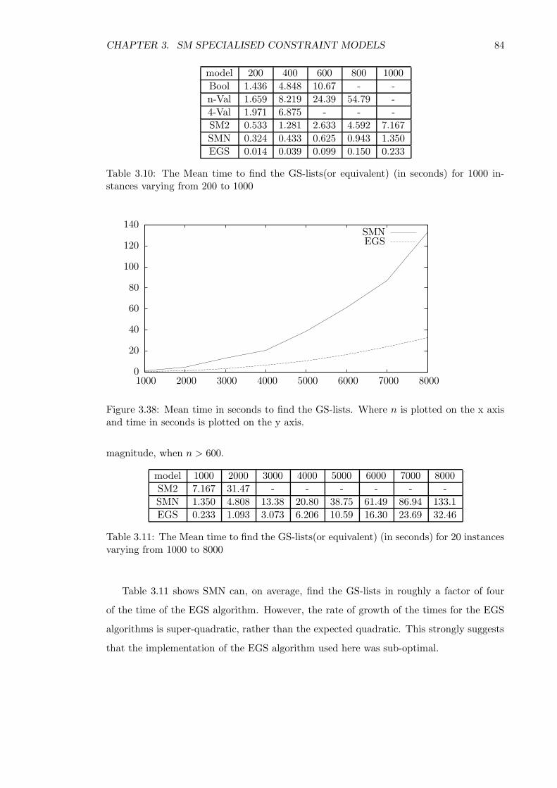
CHAPTER 3. SM SPECIALISED CONSTRAINT MODELS 84
model 200 400 600 800 1000
Bool 1.436 4.848 10.67 - -
n-Val 1.659 8.219 24.39 54.79 -
4-Val 1.971 6.875 - - -
SM2 0.533 1.281 2.633 4.592 7.167
SMN 0.324 0.433 0.625 0.943 1.350
EGS 0.014 0.039 0.099 0.150 0.233
Table 3.10: The Mean time to find the GS-lists(or equivalent) (in seconds) for 1000 in-stances varying from 200 to 1000
EGSSMN
80007000600050004000300020001000
140
120
100
80
60
40
20
0
Figure 3.38: Mean time in seconds to find the GS-lists. Where n is plotted on the x axisand time in seconds is plotted on the y axis.
magnitude, when n > 600.
model 1000 2000 3000 4000 5000 6000 7000 8000
SM2 7.167 31.47 - - - - - -
SMN 1.350 4.808 13.38 20.80 38.75 61.49 86.94 133.1
EGS 0.233 1.093 3.073 6.206 10.59 16.30 23.69 32.46
Table 3.11: The Mean time to find the GS-lists(or equivalent) (in seconds) for 20 instancesvarying from 1000 to 8000
Table 3.11 shows SMN can, on average, find the GS-lists in roughly a factor of four
of the time of the EGS algorithm. However, the rate of growth of the times for the EGS
algorithms is super-quadratic, rather than the expected quadratic. This strongly suggests
that the implementation of the EGS algorithm used here was sub-optimal.
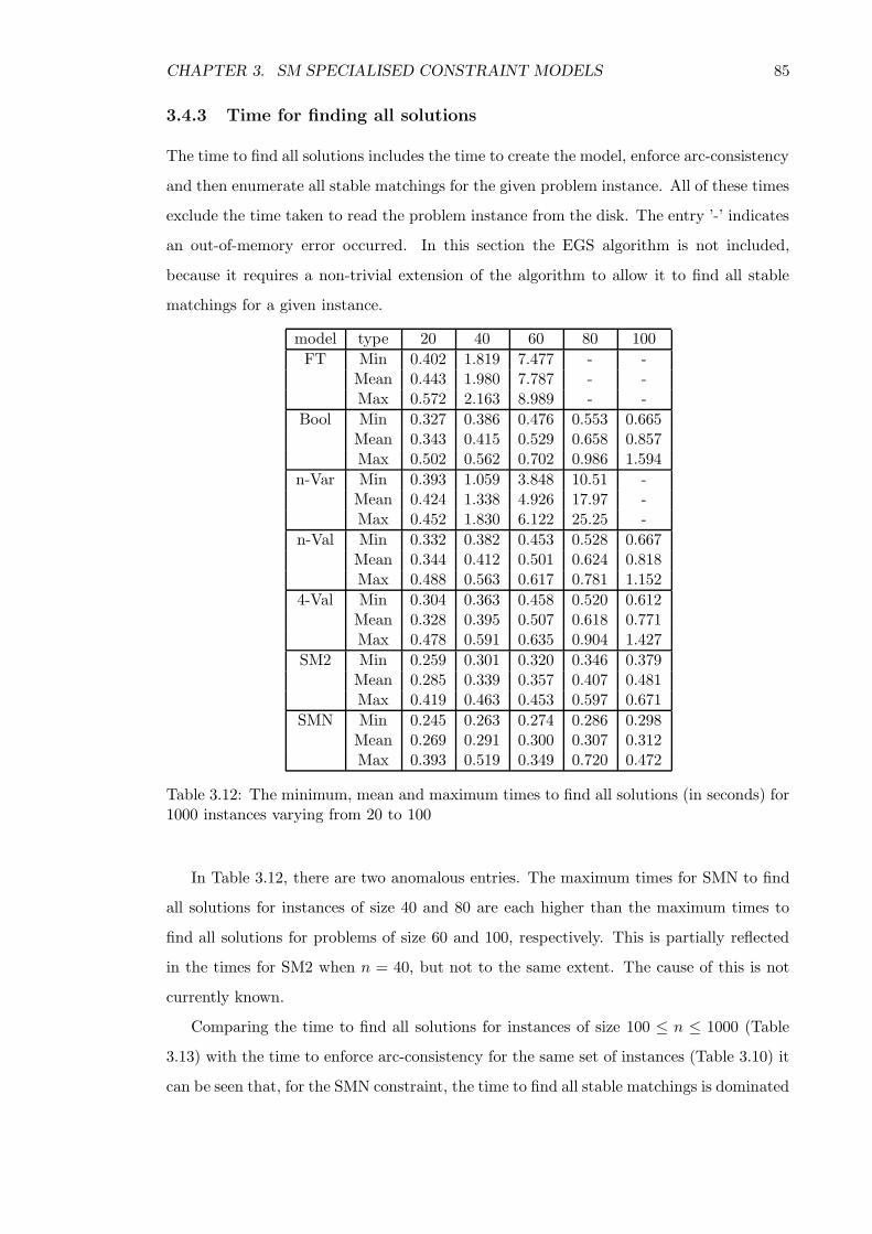
CHAPTER 3. SM SPECIALISED CONSTRAINT MODELS 85
3.4.3 Time for finding all solutions
The time to find all solutions includes the time to create the model, enforce arc-consistency
and then enumerate all stable matchings for the given problem instance. All of these times
exclude the time taken to read the problem instance from the disk. The entry ’-’ indicates
an out-of-memory error occurred. In this section the EGS algorithm is not included,
because it requires a non-trivial extension of the algorithm to allow it to find all stable
matchings for a given instance.
model type 20 40 60 80 100
FT Min 0.402 1.819 7.477 - -Mean 0.443 1.980 7.787 - -Max 0.572 2.163 8.989 - -
Bool Min 0.327 0.386 0.476 0.553 0.665Mean 0.343 0.415 0.529 0.658 0.857Max 0.502 0.562 0.702 0.986 1.594
n-Var Min 0.393 1.059 3.848 10.51 -Mean 0.424 1.338 4.926 17.97 -Max 0.452 1.830 6.122 25.25 -
n-Val Min 0.332 0.382 0.453 0.528 0.667Mean 0.344 0.412 0.501 0.624 0.818Max 0.488 0.563 0.617 0.781 1.152
4-Val Min 0.304 0.363 0.458 0.520 0.612Mean 0.328 0.395 0.507 0.618 0.771Max 0.478 0.591 0.635 0.904 1.427
SM2 Min 0.259 0.301 0.320 0.346 0.379Mean 0.285 0.339 0.357 0.407 0.481Max 0.419 0.463 0.453 0.597 0.671
SMN Min 0.245 0.263 0.274 0.286 0.298Mean 0.269 0.291 0.300 0.307 0.312Max 0.393 0.519 0.349 0.720 0.472
Table 3.12: The minimum, mean and maximum times to find all solutions (in seconds) for1000 instances varying from 20 to 100
In Table 3.12, there are two anomalous entries. The maximum times for SMN to find
all solutions for instances of size 40 and 80 are each higher than the maximum times to
find all solutions for problems of size 60 and 100, respectively. This is partially reflected
in the times for SM2 when n = 40, but not to the same extent. The cause of this is not
currently known.
Comparing the time to find all solutions for instances of size 100 ≤ n ≤ 1000 (Table
3.13) with the time to enforce arc-consistency for the same set of instances (Table 3.10) it
can be seen that, for the SMN constraint, the time to find all stable matchings is dominated
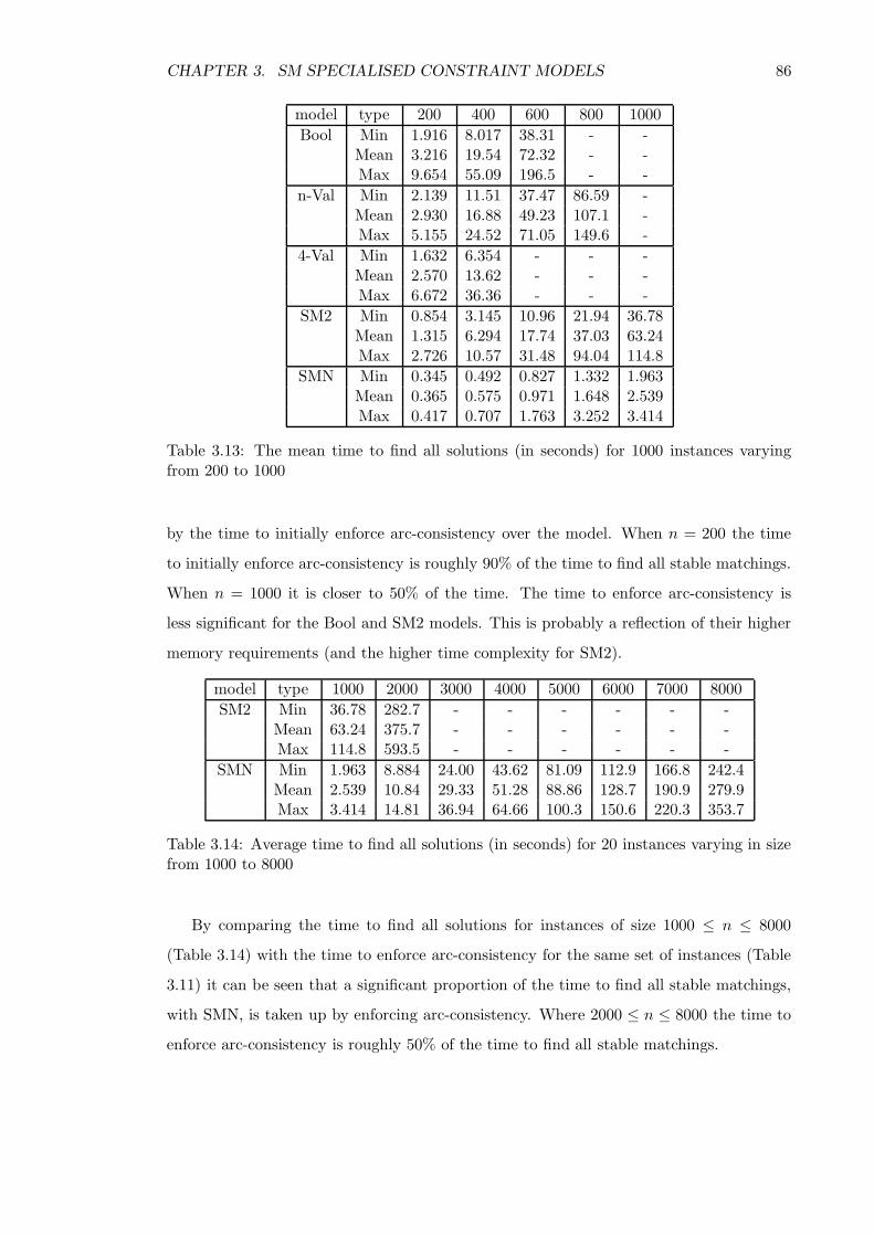
CHAPTER 3. SM SPECIALISED CONSTRAINT MODELS 86
model type 200 400 600 800 1000
Bool Min 1.916 8.017 38.31 - -Mean 3.216 19.54 72.32 - -Max 9.654 55.09 196.5 - -
n-Val Min 2.139 11.51 37.47 86.59 -Mean 2.930 16.88 49.23 107.1 -Max 5.155 24.52 71.05 149.6 -
4-Val Min 1.632 6.354 - - -Mean 2.570 13.62 - - -Max 6.672 36.36 - - -
SM2 Min 0.854 3.145 10.96 21.94 36.78Mean 1.315 6.294 17.74 37.03 63.24Max 2.726 10.57 31.48 94.04 114.8
SMN Min 0.345 0.492 0.827 1.332 1.963Mean 0.365 0.575 0.971 1.648 2.539Max 0.417 0.707 1.763 3.252 3.414
Table 3.13: The mean time to find all solutions (in seconds) for 1000 instances varyingfrom 200 to 1000
by the time to initially enforce arc-consistency over the model. When n = 200 the time
to initially enforce arc-consistency is roughly 90% of the time to find all stable matchings.
When n = 1000 it is closer to 50% of the time. The time to enforce arc-consistency is
less significant for the Bool and SM2 models. This is probably a reflection of their higher
memory requirements (and the higher time complexity for SM2).
model type 1000 2000 3000 4000 5000 6000 7000 8000
SM2 Min 36.78 282.7 - - - - - -Mean 63.24 375.7 - - - - - -Max 114.8 593.5 - - - - - -
SMN Min 1.963 8.884 24.00 43.62 81.09 112.9 166.8 242.4Mean 2.539 10.84 29.33 51.28 88.86 128.7 190.9 279.9Max 3.414 14.81 36.94 64.66 100.3 150.6 220.3 353.7
Table 3.14: Average time to find all solutions (in seconds) for 20 instances varying in sizefrom 1000 to 8000
By comparing the time to find all solutions for instances of size 1000 ≤ n ≤ 8000
(Table 3.14) with the time to enforce arc-consistency for the same set of instances (Table
3.11) it can be seen that a significant proportion of the time to find all stable matchings,
with SMN, is taken up by enforcing arc-consistency. Where 2000 ≤ n ≤ 8000 the time to
enforce arc-consistency is roughly 50% of the time to find all stable matchings.

CHAPTER 3. SM SPECIALISED CONSTRAINT MODELS 87
3.4.4 The number of solutions
20 40 60 80 100
Max 26 112 128 228 366
Mean 6 16 26 40 52
Min 1 1 2 2 7
Table 3.15: Maximum, Mean and Minimum numbers of solutions found for 1000 instancesvarying in size from 20 to 100
MaximumMean
Minimum
100908070605040302010
400
350
300
250
200
150
100
50
0
Figure 3.39: Maximum, Mean and Minimum numbers of solutions found for 1000 instancesvarying in size from 10 to 100, where n is plotted on the x axis and the number of solutionsis plotted on the y axis.
200 400 600 800 1000
Max 767 1292 2334 7160 7484
Mean 140 332 558 821 1062
Min 29 62 138 192 276
Table 3.16: Maximum, Mean and Minimum numbers of solutions found for 1000 instancesvarying in size from 200 to 1000
The number of solutions found for each SM instance was also recorded. Looking at
the number of solutions in all instances (Tables 3.15, 3.16 and 3.17) it can be seen that
the average number of solutions is increasing faster than n. The averages for instances of
size n = 2000 . . . 8000 fluctuate more than expected. This is probably a result of the low
sample size for that range of instance sizes.
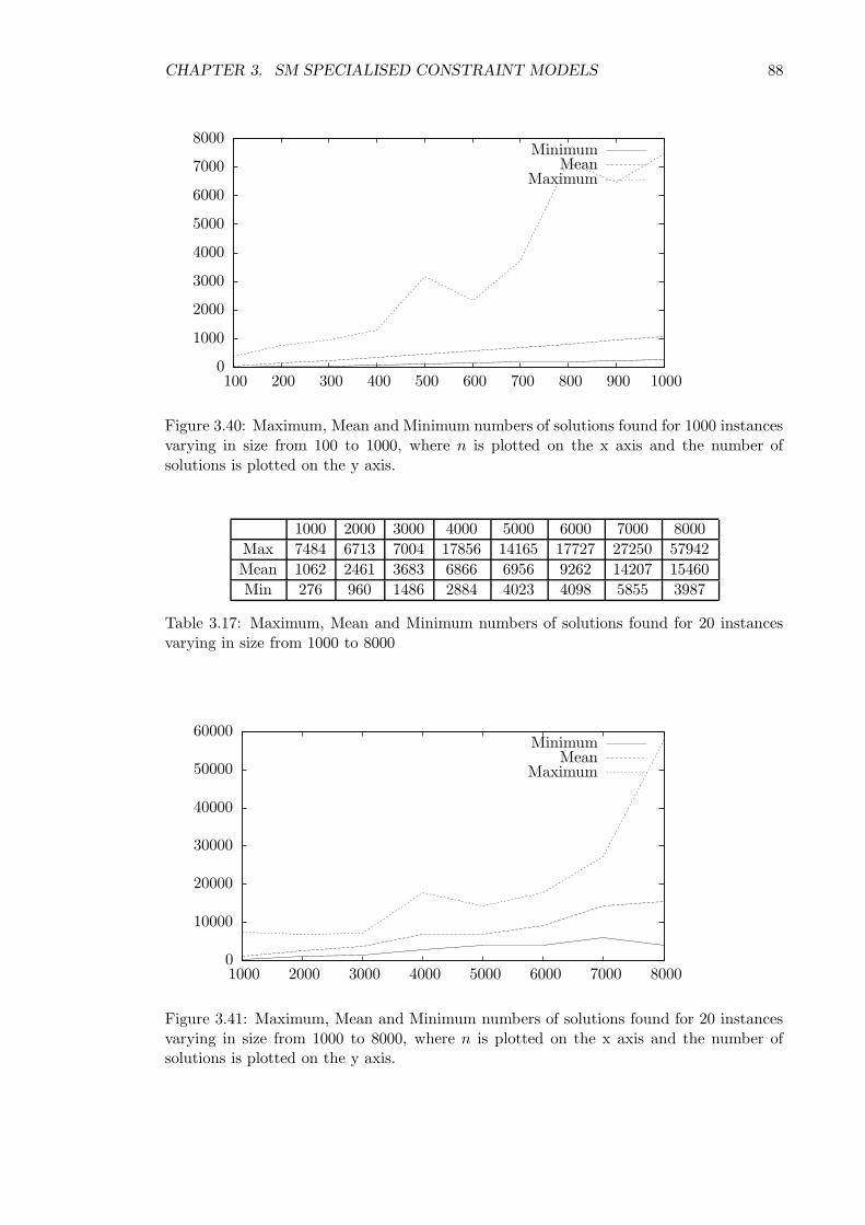
CHAPTER 3. SM SPECIALISED CONSTRAINT MODELS 88
MaximumMean
Minimum
1000900800700600500400300200100
8000
7000
6000
5000
4000
3000
2000
1000
0
Figure 3.40: Maximum, Mean and Minimum numbers of solutions found for 1000 instancesvarying in size from 100 to 1000, where n is plotted on the x axis and the number ofsolutions is plotted on the y axis.
1000 2000 3000 4000 5000 6000 7000 8000
Max 7484 6713 7004 17856 14165 17727 27250 57942
Mean 1062 2461 3683 6866 6956 9262 14207 15460
Min 276 960 1486 2884 4023 4098 5855 3987
Table 3.17: Maximum, Mean and Minimum numbers of solutions found for 20 instancesvarying in size from 1000 to 8000
MaximumMean
Minimum
80007000600050004000300020001000
60000
50000
40000
30000
20000
10000
0
Figure 3.41: Maximum, Mean and Minimum numbers of solutions found for 20 instancesvarying in size from 1000 to 8000, where n is plotted on the x axis and the number ofsolutions is plotted on the y axis.

CHAPTER 3. SM SPECIALISED CONSTRAINT MODELS 89
Comparing Tables 3.14 and 3.11, it can be seen that finding all stable matchings
after the problem is made arc-consistent, when n = 8000, takes roughly the same time
as it takes to enforce arc-consistency. It takes, in the worst case O(n2) time to enforce
arc-consistency. The instances have on average roughly 2n solutions. This gives rise to
the following conjecture about a constraint model that uses the SMN constraint. After
arc-consistency has been enforced on the constraint model, all stable matchings can be
enumerated on average in O(n ∗ s) time, where s is the number of stable matchings. To
test this conjecture Tn∗A was plotted against n in a graph, where T is the average time
to enumerate all stable matchings after enforcing arc-consistency, and A is the average
number of stable matchings in a stable marriage instance of size n.
SMN time per matching
80007000600050004000300020001000
2e-005
1.5e-005
1e-005
5e-006
0
-5e-006
-1e-005
Figure 3.42: Mean time to find all solutions divided by the average number of solutions ×n plotted on the y axis, against n on the x axis.
The graph, shown in Figure 3.42, illustrates that when n > 200 the line stabilises and
appears to remain constant, thus, supporting the conjecture that on average SMN can
enumerate all stable matchings after enforcing arc-consistency in O(n ∗ s) time, where s is
the total number of stable matchings.
3.5 Conclusion
In this chapter, two specialised constraints SM2 and SMN have been presented for the
Stable Marriage problem. It has been shown that propagating SMN will reduce the con-
strained variables to an arc-consistent state. This has been proven to be equivalent to the
GS-lists as produced by the EGS algorithm. This constraint can also be used to find all
CHAPTER 3. SM SPECIALISED CONSTRAINT MODELS 90
stable matchings for a given stable marriage instance as part of a failure free search pro-
cess. Empirical evidence has shown that both SM2 and SMN run significantly faster than
previously published toolbox constraint solutions to this problem. Furthermore, for stable
marriage instances where n is between 2000 and 8000, SMN can find the equivalent of the
GS-lists within a factor of four of the time of the implementation of the EGS algorithm
used for these experiments.

Chapter 4
Specialisations of SMN
4.1 Introduction
In this chapter, two further specialisations of the n-ary stable marriage constraint (SMN),
detailed in Chapter 3, are proposed. Both of these specialisations attempt to reduce the
memory requirements of the model. The first specialisation reduces the level of propagation
such that no internal domain value will be removed. This is done so that during search
the variable domains can be represented as a range, thus, reducing memory requirements.
The second specialisation reduces the number of variables by modelling only the male
preference lists. Empirical results are then given which show the performance increases
gained as a result of these specialisations.
4.2 Bound n-ary stable marriage constraint BSMN
In Section 3.4.1, it was shown that using O(n) variables of size n, instead of O(n2) variables
of size 2, allows larger problems to be modelled. This is because large consecutive variable
domains can be represented as a range. Thus, a domain of any size can be stored using
only two integers. If values are removed from the interior of the variable domains then
they can no longer be represented as a single range of values. Therefore, the memory
requirements to store these domains will increase. These increasing memory requirements
during search could cause either the system to slow down while it manages the extra
memory requirements or cause the search to fail due to the memory requirements exceeding
the available resources. Therefore, it would be advantageous if the propagation could be
restricted in such a way as to guarantee that no interior domain values will be removed.
91

CHAPTER 4. SPECIALISATIONS OF SMN 92
In the SMN constraint, there are only two functions that can cause a variable reduction,
the setMax function called in the stable procedure and the delV al function called from
the remV al method. The setMax function can never remove an interior domain value
and thus does not need to be altered. Therefore, the only function call that could remove
an interior domain value is the delV al function call. This function is called to remove wj ’s
preference for mi from the domain of zj+n. This call is only made after mi’s preference
for wj has been removed from the domain of zi. This means that wj has been removed
from mi’s domain and mi is, therefore, rejecting wj . The only subsequent propagation
this could cause would be if mi was wj’s previous favourite. This would force wj to make
a new proposal to her next favourite man. To ensure that no internal domain values are
removed, the delV al function should be called only on the condition that the value to be
removed is the current lowest value in the domain from which it will be removed. This
will preserve the sequence of proposals but prevent any internal domain value from being
removed. As a result, when the lower bound of a variable zi’s domain increases and a new
proposal needs to be made, the new lower bound of zi’s domain may represent a person
that has already rejected mi. This can be resolved in the stable procedure by checking
if the new lower bound is available or not. The Bound Stable Marriage n-ary constraint
(BSMN) is now described.
The BSMN constraint assumes that it has access to the following functions:
• PL(k, a) where 1 ≤ k ≤ 2n and 1 ≤ a ≤ n, will return the index of the variable
representing the ath person in the preference list of the person represented by the
variable zk.
• pref(k, l) where 1 ≤ k, l ≤ 2n, will return the rank of the person represented by
variable zl in the preference list of the person represented by zk.
• min(dom(x)) will return the smallest value remaining in the domain of variable x.
• setMax(dom(x), k) will delete all values from the domain of variable x which are
strictly greater than the value k.
• delV al(dom(x), k) will delete the value k from the domain of variable x.
BSMN is an n-ary stable marriage constraint that acts over 2n variables, which repre-
sent n men and n women, and has the following attributes:
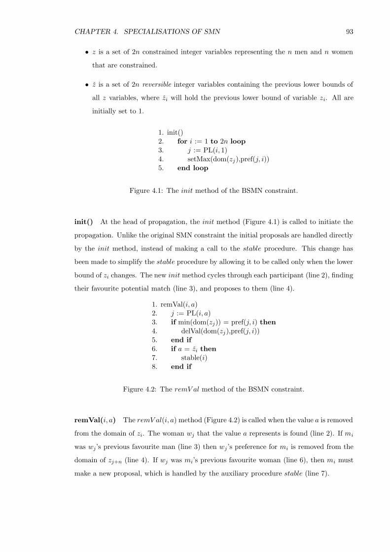
CHAPTER 4. SPECIALISATIONS OF SMN 93
• z is a set of 2n constrained integer variables representing the n men and n women
that are constrained.
• z is a set of 2n reversible integer variables containing the previous lower bounds of
all z variables, where zi will hold the previous lower bound of variable zi. All are
initially set to 1.
1. init()2. for i := 1 to 2n loop3. j := PL(i, 1)4. setMax(dom(zj),pref(j, i))5. end loop
Figure 4.1: The init method of the BSMN constraint.
init() At the head of propagation, the init method (Figure 4.1) is called to initiate the
propagation. Unlike the original SMN constraint the initial proposals are handled directly
by the init method, instead of making a call to the stable procedure. This change has
been made to simplify the stable procedure by allowing it to be called only when the lower
bound of zi changes. The new init method cycles through each participant (line 2), finding
their favourite potential match (line 3), and proposes to them (line 4).
1. remVal(i, a)2. j := PL(i, a)3. if min(dom(zj)) = pref(j, i) then4. delVal(dom(zj),pref(j, i))5. end if6. if a = zi then7. stable(i)8. end if
Figure 4.2: The remV al method of the BSMN constraint.
remVal(i, a) The remV al(i, a) method (Figure 4.2) is called when the value a is removed
from the domain of zi. The woman wj that the value a represents is found (line 2). If mi
was wj’s previous favourite man (line 3) then wj ’s preference for mi is removed from the
domain of zj+n (line 4). If wj was mi’s previous favourite woman (line 6), then mi must
make a new proposal, which is handled by the auxiliary procedure stable (line 7).

CHAPTER 4. SPECIALISATIONS OF SMN 94
1. stable(i)2. while zi 6= min(dom(zi)) loop3. zi := zi + 14. j := PL(i, zi)5. setMax(dom(zj),pref(j, i))6. if pref(j, i) > max(dom(zj)) then7. remValue(dom(zi),pref(i, j))8. end if9. end loop
Figure 4.3: The stable function of the BSMN constraint.
stable(i) The stable(i) procedure (Figure 4.3) is called via the remV al(i, a) method
when the lower bound of zi increases. While mi’s previous favourite has been removed
from his domain (line 2) then a new proposal needs to be made. zi is incremented (line
3) and mi’s favourite match, that he has not yet proposed to, wj is found (line 4) and
proposed to (line 5). If mi has previously been removed from wj ’s domain (line 6), then
wj will be removed from mi’s domain. This is then repeated until a woman is found that
still has mi in her domain (line 2).
The conditional statement on line 6 in Figure 4.3 makes the assumption that all domain
reductions will be restricted to the bounds of the variables and no interior values can be
removed. If side constraints were to be added to this model that assumption may prove
to be false. In this case, the condition in the if statement on line 6 could be changed to
“pref(j, i) /∈ dom(zj)”. However, if such side constraints were added then the property of
consecutive domains may be lost.
The level of propagation enforced by the BSMN constraint will be equivalent to that
of the optimal Bool constraint model proposed in 2001 [40] and detailed in Section 2.4.
4.2.1 Complexity of BSMN
The init method will be called once at the head of propagation. It will cycle 2n times,
each iteration will run in constant time, making the time complexity of a call to init O(n).
The remV al method is called each time a domain value is removed, thus can be called at
most 2n2 times. This method has no loops and, excluding the call to stable (which will
be handled separately), will run in constant time, making the worst case time complexity
for the total set of calls to remV al O(n2). The auxiliary function stable(i) is called via
the remV al method. It can be called at most n times for each of the 2n values of i.
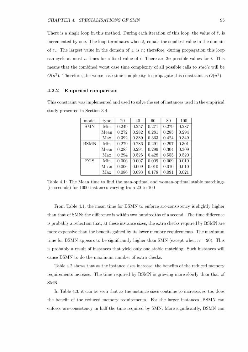
CHAPTER 4. SPECIALISATIONS OF SMN 95
There is a single loop in this method. During each iteration of this loop, the value of zi is
incremented by one. The loop terminates when zi equals the smallest value in the domain
of zi. The largest value in the domain of zi is n; therefore, during propagation this loop
can cycle at most n times for a fixed value of i. There are 2n possible values for i. This
means that the combined worst case time complexity of all possible calls to stable will be
O(n2). Therefore, the worse case time complexity to propagate this constraint is O(n2).
4.2.2 Empirical comparison
This constraint was implemented and used to solve the set of instances used in the empirical
study presented in Section 3.4.
model type 20 40 60 80 100
SMN Min 0.249 0.257 0.271 0.279 0.287Mean 0.272 0.282 0.281 0.285 0.294Max 0.392 0.389 0.363 0.424 0.349
BSMN Min 0.279 0.286 0.291 0.297 0.301Mean 0.283 0.294 0.299 0.304 0.309Max 0.294 0.525 0.428 0.555 0.520
EGS Min 0.006 0.007 0.009 0.009 0.010Mean 0.006 0.009 0.010 0.010 0.010Max 0.086 0.093 0.178 0.091 0.021
Table 4.1: The Mean time to find the man-optimal and woman-optimal stable matchings(in seconds) for 1000 instances varying from 20 to 100
From Table 4.1, the mean time for BSMN to enforce arc-consistency is slightly higher
than that of SMN; the difference is within two hundredths of a second. The time difference
is probably a reflection that, at these instance sizes, the extra checks required by BSMN are
more expensive than the benefits gained by its lower memory requirements. The maximum
time for BSMN appears to be significantly higher than SMN (except when n = 20). This
is probably a result of instances that yield only one stable matching. Such instances will
cause BSMN to do the maximum number of extra checks.
Table 4.2 shows that as the instance sizes increase, the benefits of the reduced memory
requirements increase. The time required by BSMN is growing more slowly than that of
SMN.
In Table 4.3, it can be seen that as the instance sizes continue to increase, so too does
the benefit of the reduced memory requirements. For the larger instances, BSMN can
enforce arc-consistency in half the time required by SMN. More significantly, BSMN can

CHAPTER 4. SPECIALISATIONS OF SMN 96
model type 200 400 600 800 1000
SMN Min 0.319 0.423 0.608 0.918 1.315Mean 0.324 0.433 0.625 0.943 1.350Max 0.349 0.754 1.169 1.044 1.425
BSMN Min 0.329 0.383 0.474 0.626 0.812Mean 0.334 0.390 0.489 0.649 0.846Max 0.340 0.402 0.561 0.773 0.990
EGS Min 0.013 0.037 0.078 0.142 0.224Mean 0.014 0.039 0.099 0.150 0.233Max 0.087 0.261 0.376 1.121 1.019
Table 4.2: The Mean time to find the man-optimal and woman-optimal stable matchings(in seconds) for 1000 instances varying from 200 to 1000
model type 1000 2000 3000 4000 5000 6000 7000 8000
SMN Min 1.315 4.737 12.97 20.51 37.96 60.64 85.13 131.0Mean 1.350 4.808 13.38 20.80 38.75 61.49 86.94 133.1Max 1.425 4.911 13.84 21.30 39.51 62.55 87.97 134.7
BSMN Min 0.812 2.653 5.984 10.99 18.12 27.80 39.06 51.86Mean 0.846 2.688 6.222 11.38 18.52 28.33 40.09 55.01Max 0.990 2.767 6.454 11.82 18.98 29.38 40.96 92.41
EGS Min 0.224 1.078 3.026 6.120 10.45 16.14 23.40 32.00Mean 0.233 1.093 3.073 6.206 10.59 16.30 23.69 32.46Max 1.019 1.115 3.187 6.317 10.83 16.60 23.83 33.72
Table 4.3: The Mean time to find the man-optimal and woman-optimal stable matchings(in seconds) for 20 instances varying from 1000 to 8000
enforce arc-consistency and thus find both the male and female optimal stable matchings
in less than twice the time required by the EGS algorithm.
When n is in the range of 20 to 100, the time to find all solutions with BSMN is not
significantly different to that of SMN. Table 4.4 shows that, for this range, BSMN can find
all stable matchings within three hundredths of a second of the time of SMN.
From Table 4.5 it can be seen that the difference between the minimum and maximum
times to find all solutions with BSMN is increasing with n. This is an indication of the
lower level of consistency enforced by BSMN. Each interior value that the BSMN constraint
does not remove, that would have been removed via the SMN constraint, will have to be
removed at some point during the search process, as it does not appear in any solution.
This will then cause the same value to be removed multiple times during the search, thus
reducing its efficiency. The more solutions an instance contains the bigger the search tree
and the greater impact this inefficiency will have. This is the likely cause of the larger

CHAPTER 4. SPECIALISATIONS OF SMN 97
model type 20 40 60 80 100
SMN Min 0.245 0.263 0.274 0.286 0.298Mean 0.269 0.291 0.300 0.307 0.312Max 0.393 0.519 0.349 0.720 0.472
BSMN Min 0.275 0.290 0.302 0.305 0.317Mean 0.284 0.310 0.324 0.333 0.345Max 0.344 0.528 0.421 0.413 0.459
Table 4.4: The maximum, mean, and minimum times to find all solutions (in seconds) for1000 instances varying from 20 to 100
model type 200 400 600 800 1000
SMN Min 0.345 0.492 0.827 1.332 1.963Mean 0.365 0.575 0.971 1.648 2.539Max 0.417 0.707 1.763 3.252 3.414
BSMN Min 0.370 0.505 0.905 1.387 1.944Mean 0.412 0.710 1.268 2.106 3.233Max 0.542 1.093 2.049 6.030 5.580
Table 4.5: The mean time to find all solutions (in seconds) for 1000 instances varying from200 to 1000
range of times for BSMN compared to SMN.
model type 1000 2000 3000 4000 5000 6000 7000 8000
SMN Min 1.963 8.884 24.00 43.62 81.09 112.9 166.8 242.4Mean 2.539 10.84 29.33 51.28 88.86 128.7 190.9 279.9Max 3.414 14.81 36.94 64.66 100.3 150.6 220.3 353.7
BSMN Min 1.944 9.557 30.57 52.11 87.35 122.9 190.0 257.3Mean 3.233 14.33 39.58 68.68 105.5 158.2 245.1 331.0Max 5.580 21.86 54.30 99.43 127.4 206.5 321.7 444.3
Table 4.6: Average time to find all solutions (in seconds) for 20 instances varying in sizefrom 1000 to 8000
Table 4.6 shows the large range of times recorded for the instances in the range 1000
to 8000. As with the results from the instances of size 200 to 1000, it can be seen that the
range of times was larger for BSMN than SMN.
From these empirical results it can be seen that, by ensuring no interior domain values
are removed, we can significantly improve the time to enforce arc-consistency and thus
find a stable matching. This significantly reduces the performance gap between the EGS
algorithm and the constraint solutions. The performance increase comes at a cost as it
takes slightly longer when finding all stable matchings. If side constraints were added to
this model that removed interior domain values then, depending how the solver represented
CHAPTER 4. SPECIALISATIONS OF SMN 98
the variable domains, the performance may be adversely effected. If the solver represents
only the bounds of the variable domains then any attempt to remove any inconsistent
interior domain values will have no effect. In this case the propagation will be deferred
until the inconsistent value is one of the bounds of the variable, at which time the value will
be removed. This approach will not adversely effect the runtime of the BSMN constraint.
However, it may reduce the level of consistency attained by the side constraints, which may
adversely effect the runtime. Alternately, the solver may allow side constraints to remove
interior values, which will nullify the benefits gained by BSMN and, thus, adversely effect
the runtime. These restriction will reduce the versatility of this constraint and, therefore,
its usefulness.
4.3 Compact n-ary stable marriage constraint CSMN
In 2003, Green et al [47] proposed an extensional constraint model for the Stable Marriage
problem that used only n variables with domains of length n, as opposed to all other
published constraint models to date that use either 2n or 2n2 variables. Using only n
variables will halve the number of possible domain reductions as well as significantly reduce
the memory requirements. Assuming that the effort to propagate each domain reduction
is not double that of other models, such a model should yield a significant performance
improvement. The compact n-ary stable marriage constraint (CSMN) is a specialised
constraint which acts over n variables. Enforcing arc-consistency over a constraint model
using CSMN will result in the variable domains representing the male side of the GS-lists.
From these domains, the full GS-lists can easily be constructed.
A constraint model using the SMN constraint uses a set of n variables to represent the
men and another set of n variables to represent the women. In a constraint model using
the CSMN constraint, given the domains of the male variables and the female preference
lists the domains of the female variables can be calculated. For example, if woman wj is in
the domain of man mi then mi must be in the domain of wj . More formally, if a ∈ dom(zi)
and n + j = PL(i, a) then b ∈ dom(zn+j) where i = PL(n + j, b). The CSMN constraint
eliminates this duplication by representing only the male domains. If this constraint were
implemented in a Java based constraint solver then the constructor to create a CSMN
constraint may look like CSMN(z,mpl, wpl), where z is an array of constrained integer
variables, mpl is a 2 dimensional integer array representing the male preference lists and
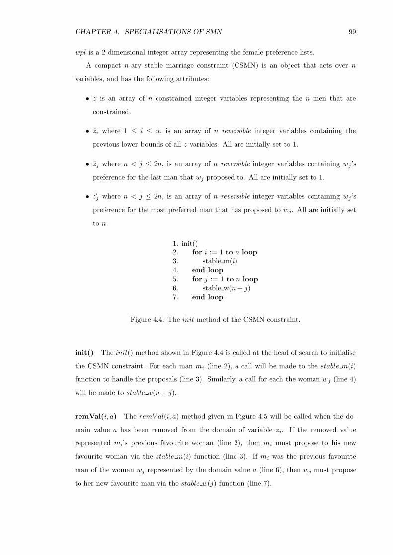
CHAPTER 4. SPECIALISATIONS OF SMN 99
wpl is a 2 dimensional integer array representing the female preference lists.
A compact n-ary stable marriage constraint (CSMN) is an object that acts over n
variables, and has the following attributes:
• z is an array of n constrained integer variables representing the n men that are
constrained.
• zi where 1 ≤ i ≤ n, is an array of n reversible integer variables containing the
previous lower bounds of all z variables. All are initially set to 1.
• zj where n < j ≤ 2n, is an array of n reversible integer variables containing wj ’s
preference for the last man that wj proposed to. All are initially set to 1.
• ~zj where n < j ≤ 2n, is an array of n reversible integer variables containing wj ’s
preference for the most preferred man that has proposed to wj. All are initially set
to n.
1. init()2. for i := 1 to n loop3. stable m(i)4. end loop5. for j := 1 to n loop6. stable w(n + j)7. end loop
Figure 4.4: The init method of the CSMN constraint.
init() The init() method shown in Figure 4.4 is called at the head of search to initialise
the CSMN constraint. For each man mi (line 2), a call will be made to the stable m(i)
function to handle the proposals (line 3). Similarly, a call for each the woman wj (line 4)
will be made to stable w(n + j).
remVal(i, a) The remV al(i, a) method given in Figure 4.5 will be called when the do-
main value a has been removed from the domain of variable zi. If the removed value
represented mi’s previous favourite woman (line 2), then mi must propose to his new
favourite woman via the stable m(i) function (line 3). If mi was the previous favourite
man of the woman wj represented by the domain value a (line 6), then wj must propose
to her new favourite man via the stable w(j) function (line 7).

CHAPTER 4. SPECIALISATIONS OF SMN 100
1. remVal(i, a)2. if a = zi then3. stable m(i)4. end if5. j := PL(i, a)6. if i = PL(j, zj) then7. stable w(j)8. end if
Figure 4.5: The remV al method of the CSMN constraint.
1. stable m(i)2. for k = zi to min(dom(zi)) loop3. j := PL(i, k)4. for l = pref(j, i) +1 to ~zj loop5. b := PL(j, l)6. delVal(dom(zb),pref(b, j))7. end loop8. ~zj := min(~zj,pref(j, i))9. end loop10. zi := min(dom(zi))
Figure 4.6: The stable m(i) function of the CSMN constraint.
stable m(i) The stable m(i) function shown in Figure 4.6 can be called to make an
initial proposal for mi via the init() method or to make a new proposal after being rejected
by a previous fiancee via the remV al(i, a) method. For each woman wj that mi has not yet
proposed to and that mi prefers to all other women in his domain (lines 2,3), a proposal
will be made. Note that if the assumption was made that CSMN has exclusive access
the the z variable domains then a proposal need only be made to mi’s current favourite
woman. When wj receives a proposal from mi she will be removed from the domains of
all men worse than mi (lines 4 to 7). After each such proposal the ~zj variable, which
holds wj’s current best proposal, will be updated (line 8). Finally, the zi variable will be
updated.
stable w(j) The stable w(j) function shown in Figure 4.7 can be called to make an ini-
tial proposal for wj−n via the init() method or to make a new proposal after being rejected
by a previous fiance via the remV al(i, a) method. Woman wj−n’s previous favourite man
mi is found (line 5) and all women worse than wj−n are removed from his domain (line
6). If the value corresponding to wj−n is still in mi’s domain (line 7) then the loop is
terminated (line 8). If wj−n has been removed from mi’s domain then we look for wj−n’s

CHAPTER 4. SPECIALISATIONS OF SMN 101
1. stable w(j)2. notDone := true3. while notDone loop4. if zj <= ~zj then5. i := PL(j, zj)6. setMax(dom(zi)),pref(i, j))7. if pref(i, j) ∈ dom(zi) then8. notDone := false9. else zj := zj + 1
10. end if11. else notDone := false12. end if13. end loop
Figure 4.7: The stable w(j) function of the CSMN constraint.
next favourite man (line 9) and wj−n proposes to him. This is then repeated until either
a man is found with wj−n still in his domain (line 8) or there are no more eligible men
(lines 4 and 11).
4.3.1 Complexity of CSMN
The init method will be called once at the head of propagation. It will cycle 2n times, each
iteration (excluding the calls to stablem and stablew which will be handled separately) will
run in constant time, making the time complexity of a call to init O(n).
The remV al method is called each time a domain value is removed, thus can be called
at most n2 times. This method has no loops and, excluding the calls to stablem and
stablew (which will be handled separately), will run in constant time, making the worst
case time complexity for the total set of calls to remV al O(n2).
The auxiliary function stablem(i) is called via the remV al and init methods. It can be
called at most n times for each of the n values of i. There is a nested loop in this function.
The number of times the inner loop will cycle is dependant on j and ~zj . Because ~zj is
initialised to n and can only decrease during propagation to a possible minimum value of
1, for all possible calls to stablem(i) for all possible values i and a fixed value of j the total
number of cycles of the inner loop is in the worst case O(n). As there are n possible values
for j and the inner loop runs in constant time, in the worst case the total time required by
the inner loop, summed over all values of i and j, will be O(n2). For each call to stablem(i)
for a fixed i the outer loop will cycle a number of times equal to the difference between
zi and min(dom(zi)). At the end of each loop zi is made equal to min(dom(zi)). As zi is

CHAPTER 4. SPECIALISATIONS OF SMN 102
initialised to 1 and min(dom(zi)) will never be greater than n, in the worst case the total
number of possible cycles of the outer loop in stablem(i) for a fixed i will be O(n). As
there are n possible values for i and the outer loop runs in constant time (excluding the
inner loop), in the worst case the total time required by the outer loop, summed over all
values of i, will be O(n2). Therefore, in the worst case, all possible calls to stablem(i) will
run in O(n2) time.
The auxiliary function stablew(j) is called via the remV al and init methods. It can
be called at most n times for each of the n values of j. This function contains a single
loop which will cycle a number of times dependant on zj . Each time the loop cycles zj
will increase by 1, up to a maximum of n times. Therefore, for a fixed value of j the loop
can, in the worst case, cycle O(n) times for all possible calls to stablew(j). As there are n
possible values for j and the loop runs in constant time, in the worst case the total time
required by the loop, summed over all values of i j, will be O(n2). Therefore, in the worst
case, all possible calls to stablew(j) will run in O(n2) time.
Therefore, the worst case time complexity to propagate the CSMN constraint is O(n2).
4.3.2 Empirical results
The CSMN constraint was implemented and used to solve the same set of instances as
used in the empirical study shown in Section 3.4.
model type 20 40 60 80 100
SMN Min 0.249 0.257 0.271 0.279 0.287Mean 0.272 0.282 0.281 0.285 0.294Max 0.392 0.389 0.363 0.424 0.349
BSMN Min 0.279 0.286 0.291 0.297 0.301Mean 0.283 0.294 0.299 0.304 0.309Max 0.294 0.525 0.428 0.555 0.520
CSMN Min 0.286 0.295 0.310 0.315 0.318Mean 0.290 0.299 0.315 0.319 0.323Max 0.375 0.306 0.403 0.405 0.422
EGS Min 0.006 0.007 0.009 0.009 0.010Mean 0.006 0.009 0.010 0.010 0.010Max 0.086 0.093 0.178 0.091 0.021
Table 4.7: The Mean time to find the man-optimal and woman-optimal stable matchings(in seconds) for 1000 instances varying from 20 to 100
From Table 4.7, it can be seen that for instances where n ≤ 100 the extra work required
to propagate CSMN outweighs the benefits gained from the smaller model size.

CHAPTER 4. SPECIALISATIONS OF SMN 103
model type 200 400 600 800 1000
SMN Min 0.319 0.423 0.608 0.918 1.315Mean 0.324 0.433 0.625 0.943 1.350Max 0.349 0.754 1.169 1.044 1.425
BSMN Min 0.329 0.383 0.474 0.626 0.812Mean 0.334 0.390 0.489 0.649 0.846Max 0.340 0.402 0.561 0.773 0.990
CSMN Min 0.353 0.438 0.589 0.821 1.152Mean 0.364 0.448 0.603 0.847 1.189Max 0.458 0.543 0.680 0.950 1.381
EGS Min 0.013 0.037 0.078 0.142 0.224Mean 0.014 0.039 0.099 0.150 0.233Max 0.087 0.261 0.376 1.121 1.019
Table 4.8: The Mean time to find the man-optimal and woman-optimal stable matchings(in seconds) for 1000 instances varying from 200 to 1000
Table 4.8 shows that for the range 200 ≤ n ≤ 1000 CSMN can be made arc-consistent
faster than the original SMN constraint. The time saved by the lower space requirements
and the reduced number of reductions by the BSMN constraint gives greater performance
benefits than the compact model of the CSMN constraint.
model type 1000 2000 3000 4000 5000 6000 7000 8000
SMN Min 1.315 4.737 12.97 20.51 37.96 60.64 85.13 131.0Mean 1.350 4.808 13.38 20.80 38.75 61.49 86.94 133.1Max 1.425 4.911 13.84 21.30 39.51 62.55 87.97 134.7
BSMN Min 0.812 2.653 5.984 10.99 18.12 27.80 39.06 51.86Mean 0.846 2.688 6.222 11.38 18.52 28.33 40.09 55.01Max 0.990 2.767 6.454 11.82 18.98 29.38 40.96 92.41
CSMN Min 1.152 4.121 9.463 17.65 28.61 54.15 64.63 105.2Mean 1.189 4.192 9.825 17.94 29.45 54.80 65.60 106.6Max 1.381 4.316 12.50 18.23 30.48 55.96 66.61 115.3
EGS Min 0.224 1.078 3.026 6.120 10.45 16.14 23.40 32.00Mean 0.233 1.093 3.073 6.206 10.59 16.30 23.69 32.46Max 1.019 1.115 3.187 6.317 10.83 16.60 23.83 33.72
Table 4.9: The Mean time to find the man-optimal and woman-optimal stable matchings(in seconds) for 20 instances varying from 1000 to 8000
It can be seen in Table 4.9 that in the range 1000 ≤ n ≤ 8000, as with the previous
ranges, the CSMN constraint slightly improves on the performance of the SMN constraint,
but the BSMN constraint model still dominates when finding a single stable matching.
Similar to finding the equivalent of the GS-lists, Table 4.10 shows that when finding
all stable matchings, the SMN constraint runs faster on instances where n ≤ 100 than

CHAPTER 4. SPECIALISATIONS OF SMN 104
model type 20 40 60 80 100
SMN Min 0.245 0.263 0.274 0.286 0.298Mean 0.269 0.291 0.300 0.307 0.312Max 0.393 0.519 0.349 0.720 0.472
BSMN Min 0.275 0.290 0.302 0.305 0.317Mean 0.284 0.310 0.324 0.333 0.345Max 0.344 0.528 0.421 0.413 0.459
CSMN Min 0.281 0.293 0.310 0.319 0.325Mean 0.286 0.304 0.328 0.339 0.350Max 0.373 0.466 0.391 0.368 0.460
Table 4.10: The maximum, mean, and minimum times to find all solutions (in seconds)for 1000 instances varying from 20 to 100
both the BSMN and CSMN constraints, with the exception of a few hard instances when
n = 40, n = 80 and n = 100.
model type 200 400 600 800 1000
SMN Min 0.345 0.492 0.827 1.332 1.963Mean 0.365 0.575 0.971 1.648 2.539Max 0.417 0.707 1.763 3.252 3.414
BSMN Min 0.370 0.505 0.905 1.387 1.944Mean 0.412 0.710 1.268 2.106 3.233Max 0.542 1.093 2.049 6.030 5.580
CSMN Min 0.379 0.498 0.749 1.113 1.565Mean 0.400 0.559 0.848 1.304 1.970Max 0.561 0.852 1.242 2.086 2.675
Table 4.11: The mean time to find all solutions (in seconds) for 1000 instances varyingfrom 200 to 1000
It can be seen in Table 4.11 that as the instance sizes grow to 200 ≤ n ≤ 1000, the
benefits of the reduced size of the CSMN constraint model start to be seen. Not only does
the CSMN constraint find all the solutions faster on average, it is also significantly more
predictable as it has a much smaller range of times than the other two constraints. During
search, the constraint solver needs to track state changes as branching decisions are made
so that, when backtracking, the previous state can be restored. The CSMN constraint
requires half the variables of either of the other two constraints, thus the time to store and
restore the state of the model during search will be significantly reduced. This benefit will
have a greater effect as the number of solutions increases, hence the CSMN constraint has
a smaller range of times.
As the instance sizes grow, Table 4.12 shows that the trend continues. This indicates

CHAPTER 4. SPECIALISATIONS OF SMN 105
model type 1000 2000 3000 4000 5000 6000 7000 8000
SMN Min 1.963 8.884 24.00 43.62 81.09 112.9 166.8 242.4Mean 2.539 10.84 29.33 51.28 88.86 128.7 190.9 279.9Max 3.414 14.81 36.94 64.66 100.3 150.6 220.3 353.7
BSMN Min 1.944 9.557 30.57 52.11 87.35 122.9 190.0 257.3Mean 3.233 14.33 39.58 68.68 105.5 158.2 245.1 331.0Max 5.580 21.86 54.30 99.43 127.4 206.5 321.7 444.3
CSMN Min 1.565 7.042 17.12 34.25 57.06 92.06 123.5 179.5Mean 1.970 8.444 21.19 40.51 62.62 104.1 144.1 206.9Max 2.675 11.71 26.24 48.27 70.24 118.4 171.6 255.8
Table 4.12: Average time to find all solutions (in seconds) for 20 instances varying in sizefrom 1000 to 8000
that CSMN is more efficient at finding all stable matchings than the other two constraints.
4.4 Conclusion
In this chapter, two further specialisations of the SMN constraint are proposed, BSMN and
CSMN. It has been shown that, by ensuring no interior domain values are removed, the
BSMN constraint is more memory efficient. It has been shown that, for larger instances,
it can find the bounds of the GS-lists, and thus a stable matching, within a factor of
two of the time required by the EGS algorithm. The CSMN constraint has shown that
using a compact model with only n variables can make the search process more efficient,
thus reducing the time to find all stable matchings. However, the benefits seen in the
BSMN and CSMN constraints come at a cost in the form of reduced versatility. Any side
constraints added to the BSMN must not remove interior domain values or the benefit of
this constraint will be lost. Any side constraints added to the CSMN constraint model
will not have direct access to the female domains. This may require additional variables
to be added to be able to express a variation on the original problem. This in turn will
reduce the advantages gained by the compact model. Therefore, in terms of versatility,
the SMN constraint is still superior to these two specialisations.

Chapter 5
A specialised constraint model for
the Hospitals/Residents problem
5.1 Introduction
The classical Hospitals/Residents problem (HR) [36] is a generalisation of the Stable Mar-
riage problem. An HR instance involves a set of n residents R = r1 . . . rn and a set of
m hospitals H = h1 . . . hm. Each resident ri ranks in order of preference a subset of
the hospitals. Each hospital hj has an associated capacity cj , such that hj can have at
most cj residents assigned to it. Each hospital hj ranks in order of preference all residents
who have hj in their preference list. The objective is to find a matching of residents to
hospitals such that each resident is matched to at most one hospital, the hospital capac-
ities are respected and the matching is stable. A matching M is stable if it contains no
blocking pairs. A (resident,hospital) pair (ri, hj) form a blocking pair if both ri and hj
improve their assignments by being matched to each other. This problem is described in
more detail in Section 2.3.5.
In this chapter, a specialised n-ary constraint HRN is introduced which can be used
to model and solve Hospitals/Residents problem instances. A constraint model using
HRN can be made arc-consistent in O(Lc) time, where L is the sum of the lengths of
all the residents’ preference lists and c is the largest of all the hospital capacities. It is
conjectured that enforcing arc-consistency over such a model is sufficient to find both the
hospital-optimal and resident-optimal stable matching. Empirical evidence is then given
to show that this constraint can solve large instances in a reasonable time.
106

CHAPTER 5. HR SPECIALISED CONSTRAINT 107
5.2 Specialised n-ary Hospitals/Residents constraint (HRN)
HRN [70] is a specialised n-ary constraint which represents an instance of the Hospi-
tals/Residents problem as a single constraint. Strictly speaking the arity of HRN is n+m,
but for simplicity it is referred to as an n-ary constraint. This constraint acts over two
arrays of constrained integer variables, x1 . . . xn, representing the residents, and y1 . . . ym,
representing the hospitals. Each resident variable xi has an initial domain of 1 . . . m.
Domain values represent preferences, meaning that if the variable xi were assigned the
value v this would represent resident ri being assigned to its vth choice hospital. Similarly,
each hospital variable yj has an initial domain of 1 . . . n, with domain values representing
preferences in the same way. In this model only the resident variables are search variables,
meaning that a solution will require all resident variables to be reduced to a single domain
value. However, the hospital variables may still have more than one value remaining in
their domains. This allows a hospital to be represented by a single variable, while still
allowing it to be matched to more than one resident.
5.2.1 The Constraint
For ease of explanation it is assumed that the problem instances this constraint will be
used to solve will have sufficient capacity in the hospitals to place all residents, and that
all residents will have complete preference lists. This means that all residents will be
matched in all stable matchings. In Section 5.2.2, it will be shown how this assumption
can be dropped.
The HRN constraint assumes that it has access to the following functions:
• PL R(k, a) will return the index of the variable representing the ath hospital in the
preference list of resident rk.
• PL H(k, a) will return the index of the variable representing the ath resident in the
preference list of hospital hk.
• pref R(i, j) will return the rank of hospital hj in the preference list of resident ri.
• pref H(j, i) will return the rank of resident ri in the preference list of hospital hj .
• min(dom(x)) will return the smallest value remaining in the domain of variable x.

CHAPTER 5. HR SPECIALISED CONSTRAINT 108
• setMax(dom(x), k) will delete all values from the domain of variable x which are
strictly greater than the value k.
• delV al(dom(x), k) will delete the value k from the domain of variable x.
• getNextHigher(dom(x), k) will return the smallest value in the domain of variable
x that is strictly greater than the value k; if no such value exists then this function
returns k.
• swap(x, y) swaps the values of the integer variables x and y.
The HRN constraint acts over a set of resident variables and a set of hospital variables,
and has the following attributes:
• x is a set of constrained integer variables representing the residents, such that resident
ri is represented by xi.
• y is a set of constrained integer variables representing the hospitals, such that hospital
hj is represented by yj.
• c is a set of integer constants containing the capacity of each hospital.
• x is a set of n reversible integer variables containing the previous lower bounds of all
x variables. All are initially set to 0. On backtracking the values in x are restored
by the solver.
• y is a set of m reversible integer variables containing the value that represents the
least favourite resident to be offered a place at the hospital. For hospital hj , yj will
equal the cthj lowest value in dom(yj). All are initially set to 0. On backtracking the
values in y are restored by the solver.
• post is an m × c array of reversible integer variables that store the applications
received by each hospital. postj is an array of length cj which contains an ordered list
of the best proposals received by hospital hj . postja contains hospital yj ’s preference
for the ath best resident to apply to hospital hj . All of the post variables are initialised
to maxInt.
As with previous constraints, the HRN constraint is designed to operate within an
AC5 like environment (as detailed in Section 2.2). This means that a method is required
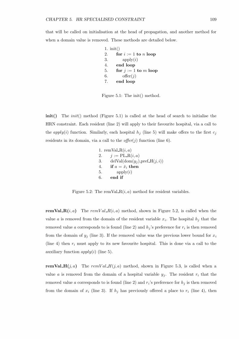
CHAPTER 5. HR SPECIALISED CONSTRAINT 109
that will be called on initialisation at the head of propagation, and another method for
when a domain value is removed. These methods are detailed below.
1. init()2. for i := 1 to n loop3. apply(i)4. end loop5. for j := 1 to m loop6. offer(j)7. end loop
Figure 5.1: The init() method.
init() The init() method (Figure 5.1) is called at the head of search to initialise the
HRN constraint. Each resident (line 2) will apply to their favourite hospital, via a call to
the apply(i) function. Similarly, each hospital hj (line 5) will make offers to the first cj
residents in its domain, via a call to the offer(j) function (line 6).
1. remVal R(i, a)2. j := PL R(i, a)3. delVal(dom(yj),pref H(j, i))4. if a = xi then5. apply(i)6. end if
Figure 5.2: The remVal R(i, a) method for resident variables.
remVal R(i, a) The remV al R(i, a) method, shown in Figure 5.2, is called when the
value a is removed from the domain of the resident variable xi. The hospital hj that the
removed value a corresponds to is found (line 2) and hj ’s preference for ri is then removed
from the domain of yj (line 3). If the removed value was the previous lower bound for xi
(line 4) then ri must apply to its new favourite hospital. This is done via a call to the
auxiliary function apply(i) (line 5).
remVal H(j, a) The remV al H(j, a) method, shown in Figure 5.3, is called when a
value a is removed from the domain of a hospital variable yj . The resident ri that the
removed value a corresponds to is found (line 2) and ri’s preference for hj is then removed
from the domain of xi (line 3). If hj has previously offered a place to ri (line 4), then

CHAPTER 5. HR SPECIALISED CONSTRAINT 110
1. remVal H(j, a)2. i := PL H(j, a)3. delVal(dom(xi),pref R(i, j))4. if a ≤ yj then5. offer(j)6. end if
Figure 5.3: The remVal H(j, a) method for hospital variables.
hj may offer a place to a new resident. This is done via a call to the auxiliary function
offer(j) (line 5).
1. apply(i)2. for k := xi + 1 to min(dom(xi)) loop3. j := PL R(i, k)4. apply(j,pref H(j, i))5. if postjcj
< maxInt then6. setMax(dom(yj),postjcj
)7. end if8. end loop9. xi := min(dom(xi))
Figure 5.4: The apply(i) function.
apply(i) The apply(i) function (Figure 5.4) can be called by either the init() method
or the remV al R(i, a) methods. This function is the residents’ equivalent of the stable(i)
function in the SMN constraint from Section 3.3. Resident ri will apply to each hospital
hj , such that ri prefers hj to any other in its domain and ri has not previously applied to
hj (line 2), note that if the assumption was made that HRN has exclusive access to the
variable domains then only a single application to the new current favourite hospital need
be made. First the hospital to be applied to, hj, is found (line 3), then resident ri makes
an application to hospital hj via a call to the apply(j, a) function(line 4). If cj applications
have been made to hospital hj (line 5) then hj must not consider any resident worse then
its cthj favourite applicant (line 6). xi is then updated with the current lower bound of xi
(line 9).
apply(j, a) The apply(j, a) function (Figure 5.5) is called by the apply(i) function. It
is called when resident ri makes an application to hospital hj (where i = PL(j, a)).
apply(j, a) maintains the array postj, which contains hj ’s preferences for the cj most

CHAPTER 5. HR SPECIALISED CONSTRAINT 111
1. apply(j, a)2. for k := 1 to cj loop3. if postjk > a then4. swap(postjk, a)5. end if6. end loop
Figure 5.5: The apply(j, a) function.
preferred residents that have applied to hj . Each element in postj is cycled through (line
2). If the current value held in postjk is greater than a (line 3) then the value of a and
postjk are swapped (line 4), meaning that postjk will become equal to a and a will be given
the previous value held in postjk. This is then repeated for the rest of the postj variables,
effectively shuffling the values down the line to reorder the list as required.
1. offer(j)2. k := min(dom(yj))3. for a := 1 to cj loop4. i := PL H(j, k)5. setMax(dom(xi),pref R(i, j))6. yj := k7. k := getNextHigher(dom(yj),k)8. end loop
Figure 5.6: The offer(j) function.
offer(j) The offer(j) function (Figure 5.6) is called by either the init() method or the
remV al H(j, a) method. This function is the hospitals’ equivalent of the stable(i) function
in the SMN constraint from Section 3.3. Hospital hj ’s most preferred resident ri is found
(lines 2 and 4), ri’s preference for all hospitals worse than hj are then removed from
dom(xi) (line 5). Hospital hj’s next favourite resident is then found (line 7). This is then
repeated cj times (line 3) at which point the top cj residents in hj ’s current domain will
have received an offer. On termination of this function, yj will be made equal to hj ’s
preference for the least preferred resident that received a proposal (line 6).
5.2.2 Enhancing the model for incomplete lists
Until now, the methods described to implement the HRN constraint have assumed that the
preference lists are complete and that there are sufficient hospital places for all residents.

CHAPTER 5. HR SPECIALISED CONSTRAINT 112
However, HRN can easily be extended to allow incomplete preference lists and insufficient
hospital places for all residents. This is achieved in much the same way as the SMN
constraint from Section 3.3.2. The value m + 1 will be added to the initial domain of
each x variable. The variable xi being assigned the value m + 1 will signify that ri is
unmatched. Similarly, the value n + 1 will be added to the initial domains of each y
variable; the value n + 1 remaining in the domain of yj indicates that hj may be assigned
less than cj residents. Additionally, the remV al R(i, a) and remV al H(j, a) methods will
not act if a is greater than m or n respectively, and lines 4 and 5 in the offer(j) function
will be run under the condition that k ≤ n. These extensions will not affect either the time
or space complexity of this constraint. This extension can also be used to model problem
instances with complete preference lists in which the hospitals have insufficient capacities
to accommodate all residents.
5.2.3 Complexity of HRN
The init() method will be called once and contains two loops, which cycle n and m times
and make calls to apply(i) and offer(j) respectively. Therefore, excluding the calls to
apply(i) and offer(j) (which will be handled separately) the init() method will run in
O(n+m) time. Neither of the two remV al methods contains loops and each can be called
at most once for each value removed from a variable domain. Therefore, excluding the
calls made to apply(i) and offer(j) (which will be handled separately) the total runtime
complexity of all calls to the two remV al methods will be O(L), where L is the sum
of the lengths of all the resident’s preference lists. For each of the m values of j the
offer(j) auxiliary function will be called once via the init() method and at most once
via the remV al H(j, a) method for each time a resident that previously received an offer
was removed from the domain of hj . This method contains one loop which will cycle cj
times. In the worst case, this method could be called once for each value in the domain
of each hospital variable, meaning that the worse case runtime complexity of all possible
calls to offer(j) for all values of j will be O(Lc). The apply(i) method makes a call to its
own auxiliary function apply(j, a) which will run in O(cj) time, making the total runtime
complexity of all possible calls to apply(i) for all values of i, O(Lc). Therefore, the total
worse case complexity to propagate a constraint model using the HRN constraint will be
O(Lc+n+m). As Lc will always dominate n+m, this will be dropped making the overall
complexity O(Lc).

CHAPTER 5. HR SPECIALISED CONSTRAINT 113
The space complexity of this encoding is dominated by the data structures used by the
pref R(i, j) and pref H(j, i) functions, which is O(nm).
5.2.4 Optimisations
The HRN constraint as proposed above can be implemented in a different way either to
optimise the constraint with respect to space or time. In both cases the optimisation
comes at a cost. The time optimisation will increase the memory requirements, while the
space optimisation will increase the time complexity of the model.
Time for space
By retaining more information about residents that apply to hospitals, the apply(j, a) and
offer(j) auxiliary functions can be re-written so that the combined time complexity of all
possible calls is reduced to O(L) time instead of its original O(Lc) time. However, the
time required to initialise the variables necessary to achieve this will make the overall time
complexity Θ(mn).
To achieve this, the original apply(i) and apply(j, a) functions and the post variables
will be replaced. The post variables will be replaced by two new integer arrays numAps
and worstAp (both initialised to 0) along with a 2 dimensional array of boolean variables
of size m×n named apps (also initialised to 0). All these new variables will be reversible,
information on previous values for these variables will be held by the solver and on back-
tracking the variables will be returned to their previous states. The new apply(i) and
apply(j, a) functions are given below in Figures 5.7 and 5.8.
1. apply(i)2. for k := xi + 1 to min(dom(xi)) loop3. j := PL R(i, k)4. apply(j,pref H(j, i))5. if numApsj ≥ cj then6. setMax(dom(yj),worstApj)7. end if8. end loop9. xi := min(dom(xi))
Figure 5.7: The apply(i) function.
apply(i) The changes to the apply(i) function, as shown in Figure 5.7, are on lines 5
and 6. If the number of applications received by hospital hj is greater than or equal to
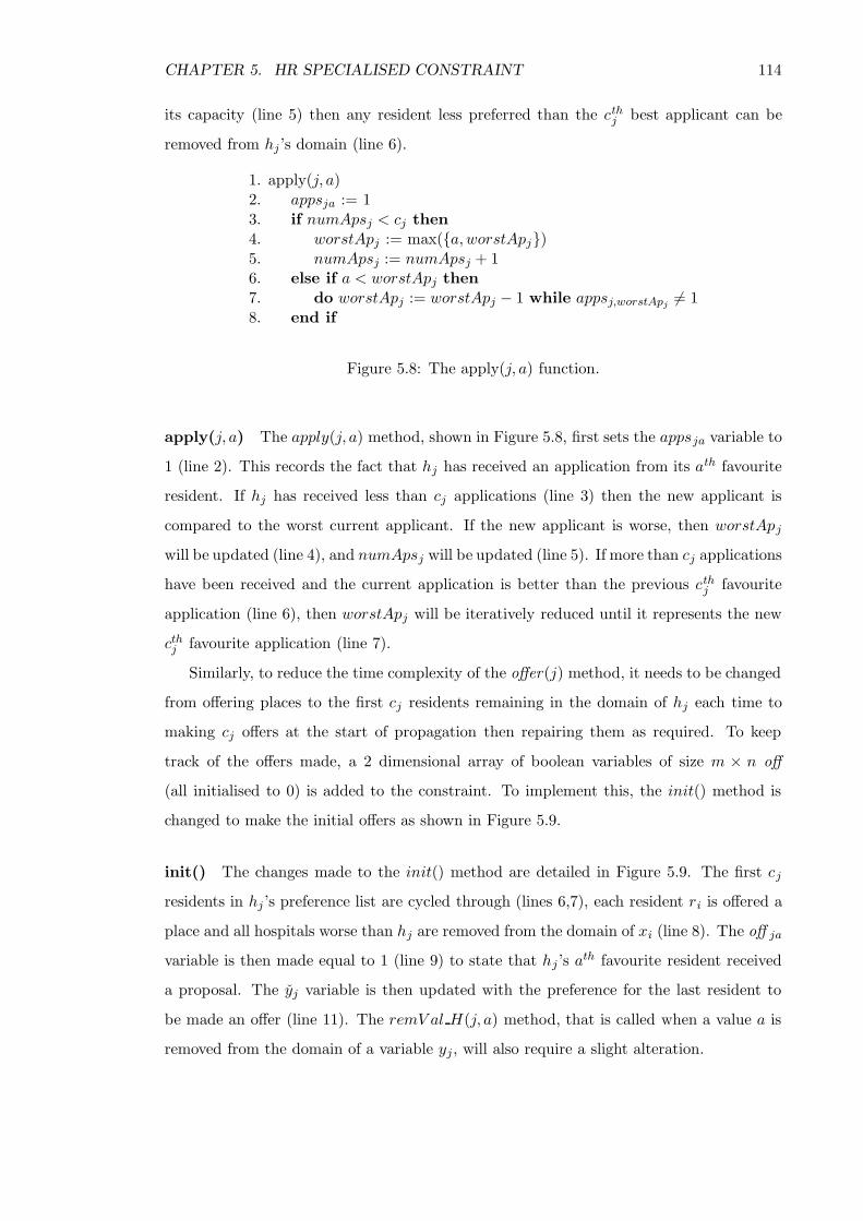
CHAPTER 5. HR SPECIALISED CONSTRAINT 114
its capacity (line 5) then any resident less preferred than the cthj best applicant can be
removed from hj ’s domain (line 6).
1. apply(j, a)2. appsja := 13. if numApsj < cj then4. worstApj := max(a,worstApj)5. numApsj := numApsj + 16. else if a < worstApj then7. do worstApj := worstApj − 1 while appsj,worstApj
6= 18. end if
Figure 5.8: The apply(j, a) function.
apply(j, a) The apply(j, a) method, shown in Figure 5.8, first sets the appsja variable to
1 (line 2). This records the fact that hj has received an application from its ath favourite
resident. If hj has received less than cj applications (line 3) then the new applicant is
compared to the worst current applicant. If the new applicant is worse, then worstApj
will be updated (line 4), and numApsj will be updated (line 5). If more than cj applications
have been received and the current application is better than the previous cthj favourite
application (line 6), then worstApj will be iteratively reduced until it represents the new
cthj favourite application (line 7).
Similarly, to reduce the time complexity of the offer(j) method, it needs to be changed
from offering places to the first cj residents remaining in the domain of hj each time to
making cj offers at the start of propagation then repairing them as required. To keep
track of the offers made, a 2 dimensional array of boolean variables of size m × n off
(all initialised to 0) is added to the constraint. To implement this, the init() method is
changed to make the initial offers as shown in Figure 5.9.
init() The changes made to the init() method are detailed in Figure 5.9. The first cj
residents in hj ’s preference list are cycled through (lines 6,7), each resident ri is offered a
place and all hospitals worse than hj are removed from the domain of xi (line 8). The off ja
variable is then made equal to 1 (line 9) to state that hj ’s ath favourite resident received
a proposal. The yj variable is then updated with the preference for the last resident to
be made an offer (line 11). The remV al H(j, a) method, that is called when a value a is
removed from the domain of a variable yj, will also require a slight alteration.

CHAPTER 5. HR SPECIALISED CONSTRAINT 115
1. init()2. for i := 1 to n loop3. apply(i)4. end loop5. for j := 1 to m loop6. for a := 1 to cj loop7. i := PL H(j, a)8. setMax(dom(xi),pref R(i, j))9. off ja := 1
10. end loop11. yj := cj
12. end loop
Figure 5.9: The init() method.
1. remVal H(j, a)2. i := PL H(j, a)3. delVal(dom(xi),pref R(i, j))4. if off ja = 1 then5. offer(j)6. end if
Figure 5.10: The remVal H(j, a) method for hospital variables.
remVal H(j, a) The small change required to the remV al H(j, a) method (detailed in
Figure 5.10), is the condition under which the offer(j) auxiliary function is called. This
function is called only when the removed value a represents a resident that has previously
received an offer (line 4). The most significant changes can be seen in the offer(j) function
detailed below.
1. offer(j)2. do loop3. yj + +4. i := PL H(j, yj)5. setMax(dom(xi),pref R(i, j))6. while yj /∈ dom(yj) or yj = lhj7. offjyj
:= 1
Figure 5.11: The offer(j) function.
offer(j) Figure 5.11 shows the revised version of the offer(j) function. Initially, the yj
variable is incremented to find the next resident to make an offer to (line 3). That resident
ri is then found (line 4), and all hospitals worse than hj are removed from its domain (line
CHAPTER 5. HR SPECIALISED CONSTRAINT 116
5). If ri was removed from hj ’s domain prior to this function call then lines 3, 4 and 5
are repeated until the best resident still in hj ’s domain yet to receive an offer is found
or the end of hj’s preference list is reached (line 6). The off variable associated to that
resident is then made equal to 1, to record that the resident received a proposal (line 7).
Any residents that were removed from hj ’s domain prior to a call to this function will not
be marked as having received an offer. This is because a value v may have been removed
from the domain of yj prior to the call to offer(j), but the call to remV al H(j, v) for that
domain reduction may still be on the call stack. In this case, if the offjv variable were
assigned the value one, when that call to remV al H(j, v) was executed, then an additional
call to offer(j) would be made, resulting in the hospital making too many offers.
Space for time
The space complexity for the HRN constraint is dominated by the data structure used to
implement the pref R(i, j) and pref H(j, i) functions in O(1) time. This is because they
require 2nm space, where n is the number of residents and m is the number of hospitals,
irrespective of the length of the preference lists. The largest known matching scheme, the
NRMP in the US [73] generally has resident preference lists with between four and seven
entries. As these matchings contain around 31,000 residents and about 2,300 hospitals, it
can be seen that the total length of the preference lists will be significantly shorter than
2nm. As such, removing the inverse preference lists will significantly reduce the memory
required to store the constraint model. This could be achieved by implementing some
kind of smart data structure such as a hash table. Alternatively, the pref R(i, j) function
could search the preference list of ri to find the position of hj within it. The runtime of
such a function will be dependent on the length of the preference lists.
5.3 Empirical study
The above constraints were implemented and used to solve Hospitals/Residents instances
randomly generated by the instance generator detailed in Appendix B.2. Since most of
the “real-life” matching schemes have short preference lists relative to the number of
participants it was decided that the problem instances generated would have residents’
preference lists of uniform length 10. The Hospitals’ preference lists are of variable length,
dependent on the number of residents that have that hospital in their preference list.

CHAPTER 5. HR SPECIALISED CONSTRAINT 117
The sizes of the instances generated are classified by the triple n/m/c, where n is the
number of residents, m is the number of hospitals and c is the uniform capacity of the
hospitals. A sample size of 100 was used for each instance size. Due to the limited length
preference lists used in this study, the HRN constraint was implemented with the space
optimisations detailed in Section 5.2.4. For comparison, the standard constraint based
model (CBM) detailed in Section 2.4.1 was also implement. Included in this study were
naive implementations of the algorithmic solutions to this problem. However, the results
returned by these naive implementations showed the specialised constraint solutions out
performed the algorithmic solutions. This result was assumed to be due to the poor
implementation of the algorithms and not a true reflection of the algorithms themselves.
For this reason, these results have been omitted from this section. This study was carried
out on a Pentium 4 2.8Ghz processor with 512 megabytes of random access memory,
running Microsoft Windows XP Professional and Java2 SDK 1.4.2.6 with an increased
heap size of 512 megabytes.
model 50/13/4 100/20/5 200/35/6 500/63/8 1K/100/10 5K/250/20
CBM 0.24 0.36 0.65 1.69 4.75 -
HRN 0.12 0.15 0.16 0.19 0.22 0.53
Table 5.1: The mean time to find all stable matchings for Hospitals/Residents instances(in seconds) for 100 instances
Figure 5.1 shows the mean time in seconds for the two encodings for varying problem
size. A table entry of − signifies that there was insufficient space to create the model of
that size using the specified encoding.
model 20K/550/37 50K/1.2K/42 200K/3K/67 500K/11.8K/85
HRN 1.42 4.2 22 35
Table 5.2: The mean time to find all stable matchings for Hospitals/Residents instances(in seconds) for 100 instances
Instances of the NRMP in the US [73] typically have around 31,000 residents and
2,300 hospitals with residents preference lists of size between 4 and 7. From Table 5.2
a constraint model using the HRN constraint can finds all stable matchings to problem
instances of size 200k/3k/67 in around 22 seconds. This indicates that this constraint
solution is a potentially suitable technology to solve this problem.
The HRN model was also used to find stable matchings for three anonymised instances
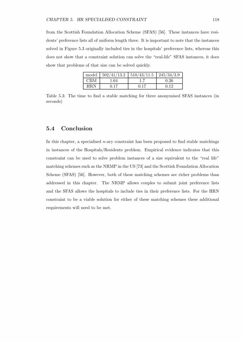
CHAPTER 5. HR SPECIALISED CONSTRAINT 118
from the Scottish Foundation Allocation Scheme (SFAS) [56]. These instances have resi-
dents’ preference lists all of uniform length three. It is important to note that the instances
solved in Figure 5.3 originally included ties in the hospitals’ preference lists, whereas this
does not show that a constraint solution can solve the “real-life” SFAS instances, it does
show that problems of that size can be solved quickly.
model 502/41/13.2 510/43/11.5 245/34/3.9
CBM 1.64 1.7 0.26
HRN 0.17 0.17 0.12
Table 5.3: The time to find a stable matching for three anonymised SFAS instances (inseconds)
5.4 Conclusion
In this chapter, a specialised n-ary constraint has been proposed to find stable matchings
in instances of the Hospitals/Residents problem. Empirical evidence indicates that this
constraint can be used to solve problem instances of a size equivalent to the “real life”
matching schemes such as the NRMP in the US [73] and the Scottish Foundation Allocation
Scheme (SFAS) [56]. However, both of these matching schemes are richer problems than
addressed in this chapter. The NRMP allows couples to submit joint preference lists
and the SFAS allows the hospitals to include ties in their preference lists. For the HRN
constraint to be a viable solution for either of these matching schemes these additional
requirements will need to be met.

Chapter 6
Versatility
Empirical evidence has shown that specialised constraint solutions to stable matching
problems can come close to the performance of the specialised algorithms, but they do
not match them. This chapter illustrates the benefits of these constraint solutions by
demonstrating their versatility. To this end a number of variants of stable matching
problems are considered and it is shown how they can be represented and solved by adding
simple side constraints to the previously presented specialised constraint models. The
variants explored in this chapter all place some extra criteria on the classical matching
problems. These problems either seek some notion of an optimal matching, according to
a given criterion, or attempt to find a matching which fulfils additional criteria. Most
of the models presented in this chapter have been implemented and empirically tested.
Statistical information about the results of these empirical studies is also given to provide
insight into the structure of the problems that have been investigated1. The problems
detailed in sections 6.6, 6.7 and 6.8 are included to show how these problems can be
modelled, but these problems will not be empirically evaluated.
6.1 The sex-equal stable marriage problem
6.1.1 The problem
The sex-equal stable marriage problem as posed by Gusfield et al.[49] as an open problem,
is essentially an optimisation problem. In the man-optimal solution to an instance of SM,
all men will be matched to their best possible partner from all possible stable matchings
1These empirical studies were carried out using the JSolver toolkit [2], i.e. the Java version of ILOGSolver, on a 3.2Ghz processor system with 2 Gb of random access memory, running Linux and Java2 SDK1.5.0.3 with an increased heap size of 1850 Mb.
119
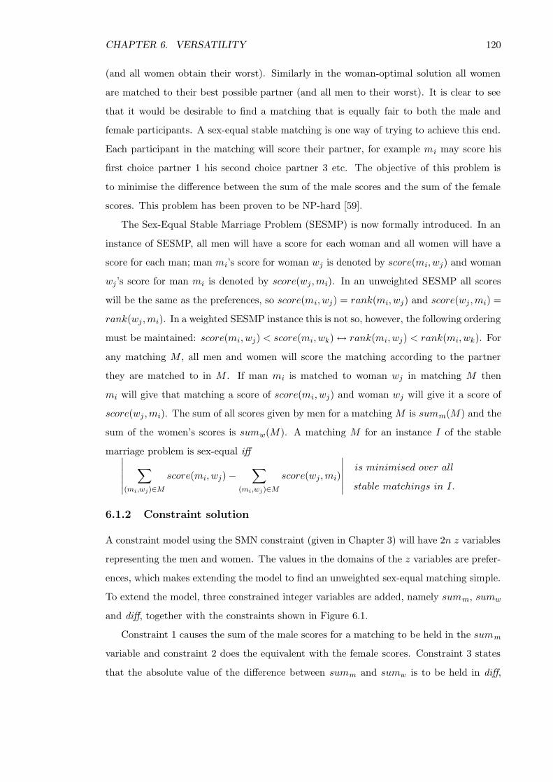
CHAPTER 6. VERSATILITY 120
(and all women obtain their worst). Similarly in the woman-optimal solution all women
are matched to their best possible partner (and all men to their worst). It is clear to see
that it would be desirable to find a matching that is equally fair to both the male and
female participants. A sex-equal stable matching is one way of trying to achieve this end.
Each participant in the matching will score their partner, for example mi may score his
first choice partner 1 his second choice partner 3 etc. The objective of this problem is
to minimise the difference between the sum of the male scores and the sum of the female
scores. This problem has been proven to be NP-hard [59].
The Sex-Equal Stable Marriage Problem (SESMP) is now formally introduced. In an
instance of SESMP, all men will have a score for each woman and all women will have a
score for each man; man mi’s score for woman wj is denoted by score(mi, wj) and woman
wj’s score for man mi is denoted by score(wj ,mi). In an unweighted SESMP all scores
will be the same as the preferences, so score(mi, wj) = rank(mi, wj) and score(wj,mi) =
rank(wj,mi). In a weighted SESMP instance this is not so, however, the following ordering
must be maintained: score(mi, wj) < score(mi, wk) ↔ rank(mi, wj) < rank(mi, wk). For
any matching M , all men and women will score the matching according to the partner
they are matched to in M . If man mi is matched to woman wj in matching M then
mi will give that matching a score of score(mi, wj) and woman wj will give it a score of
score(wj ,mi). The sum of all scores given by men for a matching M is summ(M) and the
sum of the women’s scores is sumw(M). A matching M for an instance I of the stable
marriage problem is sex-equal iff∣
∣
∣
∣
∣
∣
∑
(mi,wj)∈M
score(mi, wj) −∑
(mi,wj)∈M
score(wj ,mi)
∣
∣
∣
∣
∣
∣
is minimised over all
stable matchings in I.
6.1.2 Constraint solution
A constraint model using the SMN constraint (given in Chapter 3) will have 2n z variables
representing the men and women. The values in the domains of the z variables are prefer-
ences, which makes extending the model to find an unweighted sex-equal matching simple.
To extend the model, three constrained integer variables are added, namely summ, sumw
and diff, together with the constraints shown in Figure 6.1.
Constraint 1 causes the sum of the male scores for a matching to be held in the summ
variable and constraint 2 does the equivalent with the female scores. Constraint 3 states
that the absolute value of the difference between summ and sumw is to be held in diff,

CHAPTER 6. VERSATILITY 121
1. summ =
n∑
i=1
zi
2. sumw =2n∑
j=n+1
zj
3. diff = abs(summ − sumw)4. minimise(diff)
Figure 6.1: Side constraints for the unweighted sex-equal stable marriage problem.
where abs(a − b) returns the absolute value of the difference between a and b. Finally,
constraint 4 is a search objective to minimise diff.
To model the weighted sex-equal matching problem two sets of n variables weight m
and weight w can be added along with the constraints shown in Figure 6.2.
1. weight mi = score(mi, wj) ↔ zi = rank(mi, wj)|1 ≤ i ≤ n ∧ 1 ≤ j ≤ n2. weight wj = score(wj ,mi) ↔ zj+n = rank(wj,mi)|1 ≤ j ≤ n ∧ 1 ≤ i ≤ n
3. summ =n
∑
i=1
weight mi
4. sumw =
n∑
j=1
weight wj
5. diff = abs(summ − sumw)6. minimise(diff)
Figure 6.2: Side constraints for the weighted sex-equal stable marriage problem.
The sets of constraints labelled 1 and 2 ensure that mi’s weight for the matching is
held in the variable weight mi and wj ’s weight for the matching is held in the variable
weight wj. Constraints 3 and 4 state that the sum of the weights are to be held in the
variables summ and sumw, respectively. Constraint 5 is the same as constraint 3 in the
unweighted case. Constraint 6 is a search objective to minimise the value held in the diff
variable.
6.1.3 Empirical study
The unweighted model was implemented with the SMN constraint and tested on the same
randomly generated SM instances used in the empirical study detailed in Section 3.4.
These instances were generated by the generator detailed in Appendix B.1. The instances
used were of sizes n = 200 . . . 1000 with a sample size of 1000 for each n. Statistics about
the number of solutions contained in the instances used are shown in Table 6.1.
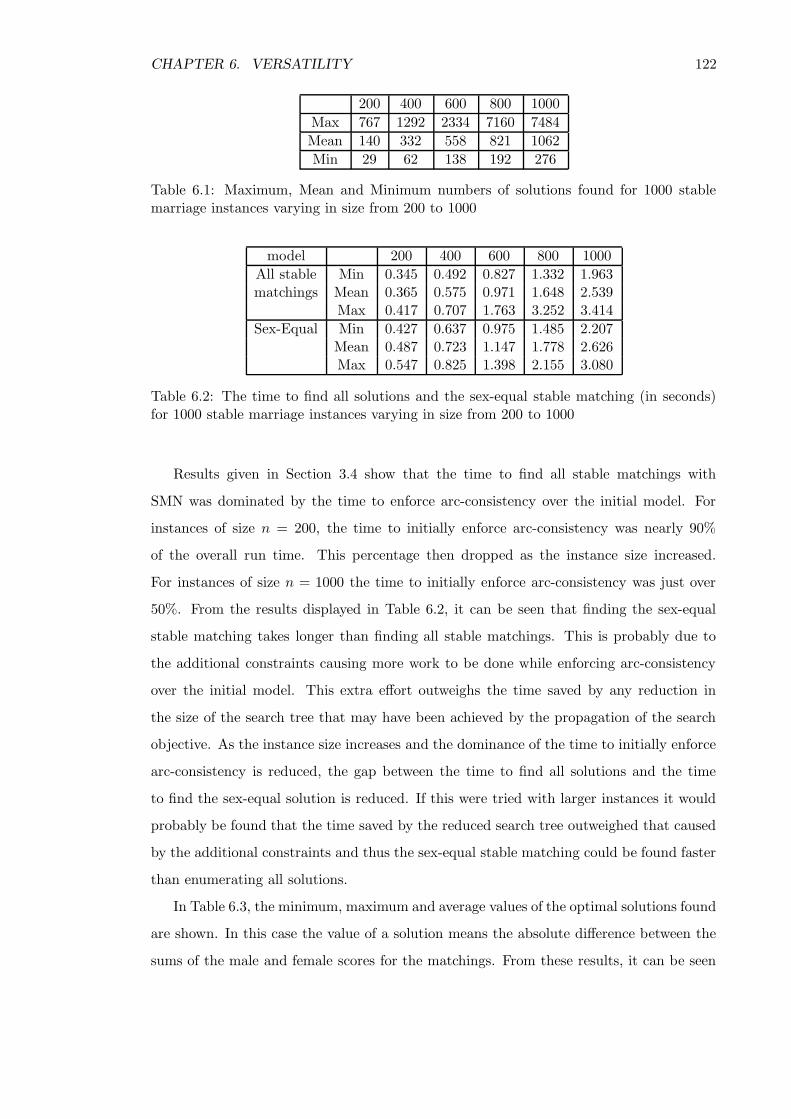
CHAPTER 6. VERSATILITY 122
200 400 600 800 1000
Max 767 1292 2334 7160 7484
Mean 140 332 558 821 1062
Min 29 62 138 192 276
Table 6.1: Maximum, Mean and Minimum numbers of solutions found for 1000 stablemarriage instances varying in size from 200 to 1000
model 200 400 600 800 1000
All stable Min 0.345 0.492 0.827 1.332 1.963matchings Mean 0.365 0.575 0.971 1.648 2.539
Max 0.417 0.707 1.763 3.252 3.414
Sex-Equal Min 0.427 0.637 0.975 1.485 2.207Mean 0.487 0.723 1.147 1.778 2.626Max 0.547 0.825 1.398 2.155 3.080
Table 6.2: The time to find all solutions and the sex-equal stable matching (in seconds)for 1000 stable marriage instances varying in size from 200 to 1000
Results given in Section 3.4 show that the time to find all stable matchings with
SMN was dominated by the time to enforce arc-consistency over the initial model. For
instances of size n = 200, the time to initially enforce arc-consistency was nearly 90%
of the overall run time. This percentage then dropped as the instance size increased.
For instances of size n = 1000 the time to initially enforce arc-consistency was just over
50%. From the results displayed in Table 6.2, it can be seen that finding the sex-equal
stable matching takes longer than finding all stable matchings. This is probably due to
the additional constraints causing more work to be done while enforcing arc-consistency
over the initial model. This extra effort outweighs the time saved by any reduction in
the size of the search tree that may have been achieved by the propagation of the search
objective. As the instance size increases and the dominance of the time to initially enforce
arc-consistency is reduced, the gap between the time to find all solutions and the time
to find the sex-equal solution is reduced. If this were tried with larger instances it would
probably be found that the time saved by the reduced search tree outweighed that caused
by the additional constraints and thus the sex-equal stable matching could be found faster
than enumerating all solutions.
In Table 6.3, the minimum, maximum and average values of the optimal solutions found
are shown. In this case the value of a solution means the absolute difference between the
sums of the male and female scores for the matchings. From these results, it can be seen

CHAPTER 6. VERSATILITY 123
200 400 600 800 1000
Minimum 0 0 0 0 0
Mean 61.55 116.3 166.8 225.5 294.1
Median 35 64 73 107.5 132.5
Maximum 504 933 1255 1716 2207
Table 6.3: Values of sex-equal stable matchings for 1000 instances varying in size from 200to 1000
that a perfect sex-equal stable matching (meaning there was no difference between the
two sums) was found for at least one instance from each of the sample sizes. The mean
value was fairly constant at around thirty percent of n, whereas the median value was
around eighteen percent of n for the smaller instances and dropped to thirteen percent
as the instance size grew to n = 1000. This indicates that a majority of stable marriage
instances contain a good sex-equal matching in which neither side is strongly favoured
against the other. However, from the maximum values it can be concluded that some
stable marriage instances do not contain a very well balanced sex-equal stable matching.
6.2 Balanced stable matching
6.2.1 The problem
The balanced stable matching problem is similar to the sex-equal stable matching problem.
The difference between the two is that instead of finding a matching which is equally good
for both the men and the women, the balanced stable matching problem seeks to find
a matching which is best for whichever group is worst off. To achieve this, assuming
that each participant scores the matching in the same way as the sex-equal problem, the
objective is to minimise the maximum of the sums of the male and female scores for the
matching. This has been proven to be an NP-hard problem [32].
The Balanced Stable Matching Problem (BSMP) is now formally introduced. In an
instance of BSMP, for a matching M , all men and women will score the matching according
to the partner they are matched to in M . If man mi is matched to woman wj in matching
M then mi will give that matching a score of rank(mi, wj) and woman wj will give it a score
of rank(wj,mi). The sum of all scores given by men for a matching M equals summ(M)
and the sum of the women’s scores is sumw(M). A matching M for an instance I of the
stable marriage problem is balanced iff
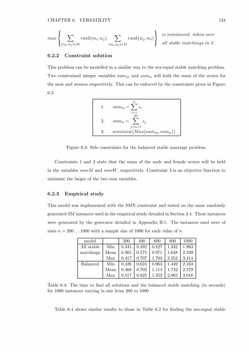
CHAPTER 6. VERSATILITY 124
max
∑
(mi,wj)∈M
rank(mi, wj),∑
(mi ,wj)∈M
rank(wj,mi)
is minimised, taken over
all stable matchings in I.
6.2.2 Constraint solution
This problem can be modelled in a similar way to the sex-equal stable matching problem.
Two constrained integer variables summ and sumw will hold the sums of the scores for
the men and women respectively. This can be enforced by the constraints given in Figure
6.3.
1. summ =
n∑
i=1
zi
2. sumw =2n∑
j=n+1
zj
3. minimise(Max(summ, sumw))
Figure 6.3: Side constraints for the balanced stable marriage problem.
Constraints 1 and 2 state that the sums of the male and female scores will be held
in the variables sumM and sumW , respectively. Constraint 3 is an objective function to
minimise the larger of the two sum variables.
6.2.3 Empirical study
This model was implemented with the SMN constraint and tested on the same randomly
generated SM instances used in the empirical study detailed in Section 3.4. These instances
were generated by the generator detailed in Appendix B.1. The instances used were of
sizes n = 200 . . . 1000 with a sample size of 1000 for each value of n.
model 200 400 600 800 1000
All stable Min 0.345 0.492 0.827 1.332 1.963matchings Mean 0.365 0.575 0.971 1.648 2.539
Max 0.417 0.707 1.763 3.252 3.414
Balanced Min 0.426 0.624 0.963 1.449 2.163Mean 0.468 0.702 1.114 1.732 2.579Max 0.517 0.825 1.352 2.065 3.016
Table 6.4: The time to find all solutions and the balanced stable matching (in seconds)for 1000 instances varying in size from 200 to 1000
Table 6.4 shows similar results to those in Table 6.2 for finding the sex-equal stable

CHAPTER 6. VERSATILITY 125
matching. When finding all solutions with the SMN constraint using the variable and value
ordering heuristic of choose some man and assign him his first choice available partner, the
first matching to be returned will be the man-optimal stable matching, which will have the
lowest sum of the male scores from all possible matchings. For each subsequent matching
returned there will be a trend that will see the sum of the male scores increase until the
final matching is returned, which will be the women-optimal matching. Given that neither
of the extremes is likely to be either balanced or sex-equal, it is fair to assume both the
balanced and sex-equal matchings are likely to be one of the matchings returned in the
middle of the enumeration. Given that assumption and the similarity of the two models,
it is unsurprising that the performance of the two models is so similar. Comparing the
results for finding the balanced and sex-equal stable matching shown in Tables 6.4 and
6.2 respectively, it can be seen that a balanced stable matching can consistently be found
slightly quicker. This suggests that either the max(a, b) function is slightly more efficient
or provides stronger propagation than the abs(a − b) function.
200 400 600 800 1000
Minimum 2495 7457 13744 21281 30170
Mean 2839 8029 14747 22690 31707
Median 2840 8027 14752 22694 31721
Maximum 3255 8690 15763 23889 33305
Table 6.5: Values of balanced stable matchings for 1000 instances varying in size from 200to 1000
In Table 6.5 it can be seen that the variation in the quality of the balanced stable
matchings found for these sets of instances reduces as the instance sizes increase.
Given the similar times to find both the sex-equal and balanced stable matchings, a
comparison of the quality of the solutions, with regard to the other problem’s criteria, was
performed. This comparison asked the questions, how balanced is the sex-equal matching?
And, how sex-equal is the balanced matching? To measure this the maximum of the sums
of the male and female matchings were recorded for the sex-equal stable matching, as was
the difference between the two sums for the balanced stable matchings. These values were
then compared to the optimal values in each case. These results are summarised in Table
6.6.
Table 6.6 shows that for more than 75% of all the instances the sex-equal and balanced
matchings were in fact the same matching. For the instances in which these matchings
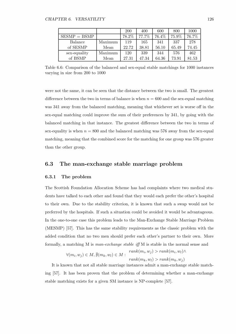
CHAPTER 6. VERSATILITY 126
200 400 600 800 1000
SESMP = BSMP 78.2% 77.7% 76.4% 75.9% 76.7%
Balance Maximum 119 165 341 337 278of SESMP Mean 22.72 38.81 56.10 65.49 74.45
sex-equality Maximum 120 339 344 576 462of BSMP Mean 27.31 47.34 64.36 73.91 81.53
Table 6.6: Comparison of the balanced and sex-equal stable matchings for 1000 instancesvarying in size from 200 to 1000
were not the same, it can be seen that the distance between the two is small. The greatest
difference between the two in terms of balance is when n = 600 and the sex-equal matching
was 341 away from the balanced matching, meaning that whichever set is worse off in the
sex-equal matching could improve the sum of their preferences by 341, by going with the
balanced matching in that instance. The greatest difference between the two in terms of
sex-equality is when n = 800 and the balanced matching was 576 away from the sex-equal
matching, meaning that the combined score for the matching for one group was 576 greater
than the other group.
6.3 The man-exchange stable marriage problem
6.3.1 The problem
The Scottish Foundation Allocation Scheme has had complaints where two medical stu-
dents have talked to each other and found that they would each prefer the other’s hospital
to their own. Due to the stability criterion, it is known that such a swap would not be
preferred by the hospitals. If such a situation could be avoided it would be advantageous.
In the one-to-one case this problem leads to the Man-Exchange Stable Marriage Problem
(MESMP) [57]. This has the same stability requirements as the classic problem with the
added condition that no two men should prefer each other’s partner to their own. More
formally, a matching M is man-exchange stable iff M is stable in the normal sense and
∀(mi, wj) ∈ M, @(mk, wl) ∈ M :rank(mi, wj) > rank(mi, wl)∧
rank(mk, wl) > rank(mk, wj)
It is known that not all stable marriage instances admit a man-exchange stable match-
ing [57]. It has been proven that the problem of determining whether a man-exchange
stable matching exists for a given SM instance is NP-complete [57].
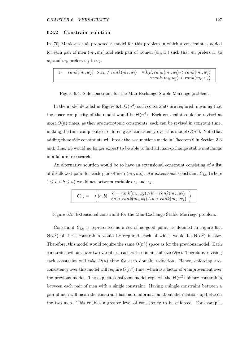
CHAPTER 6. VERSATILITY 127
6.3.2 Constraint solution
In [70] Manlove et al. proposed a model for this problem in which a constraint is added
for each pair of men (mi,mk) and each pair of women (wj , wl) such that mi prefers wl to
wj and mk prefers wj to wl.
zi = rank(mi, wj) ⇒ xk 6= rank(mk, wl) ∀ikjl, rank(mi, wl) < rank(mi, wj)∧rank(mk, wj) < rank(mk, wl)
Figure 6.4: Side constraint for the Man-Exchange Stable Marriage problem.
In the model detailed in Figure 6.4, Θ(n4) such constraints are required; meaning that
the space complexity of the model would be Θ(n4). Each constraint could be revised at
most O(n) times, as they are monotonic constraints, each can be revised in constant time,
making the time complexity of enforcing arc-consistency over this model O(n5). Note that
adding these side constraints will break the assumptions made in Theorem 9 in Section 3.3
and, thus, we would no longer expect to be able to find all man-exchange stable matchings
in a failure free search.
An alternative solution would be to have an extensional constraint consisting of a list
of disallowed pairs for each pair of men (mi,mk). An extensional constraint Ci,k (where
1 ≤ i < k ≤ n) would act between variables zi and zk.
Ci,k =
(a, b)|a = rank(mi, wj) ∧ b = rank(mk, wl)∧a > rank(mi, wl) ∧ b > rank(mk, wj)
Figure 6.5: Extensional constraint for the Man-Exchange Stable Marriage problem.
Constraint Ci,k is represented as a set of no-good pairs, as detailed in Figure 6.5.
Θ(n2) of these constraints would be required, each of which would be Θ(n2) in size.
Therefore, this model would require the same Θ(n4) space as for the previous model. Each
constraint will act over two variables, each with domains of size O(n). Therefore, revising
each constraint will take O(n) time for each domain reduction. Hence, enforcing arc-
consistency over this model will require O(n4) time, which is a factor of n improvement over
the previous model. The explicit constraint model replaces the Θ(n2) binary constraints
between each pair of men with a single constraint. Having a single constraint between a
pair of men will mean the constraint has more information about the relationship between
the two men. This enables a greater level of consistency to be enforced. For example,
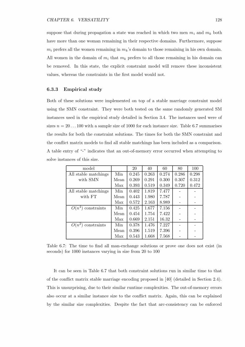
CHAPTER 6. VERSATILITY 128
suppose that during propagation a state was reached in which two men mi and mk both
have more than one woman remaining in their respective domains. Furthermore, suppose
mi prefers all the women remaining in mk’s domain to those remaining in his own domain.
All women in the domain of mi that mk prefers to all those remaining in his domain can
be removed. In this state, the explicit constraint model will remove these inconsistent
values, whereas the constraints in the first model would not.
6.3.3 Empirical study
Both of these solutions were implemented on top of a stable marriage constraint model
using the SMN constraint. They were both tested on the same randomly generated SM
instances used in the empirical study detailed in Section 3.4. The instances used were of
sizes n = 20 . . . 100 with a sample size of 1000 for each instance size. Table 6.7 summarises
the results for both the constraint solutions. The times for both the SMN constraint and
the conflict matrix models to find all stable matchings has been included as a comparison.
A table entry of “-” indicates that an out-of-memory error occurred when attempting to
solve instances of this size.
model 20 40 60 80 100
All stable matchings Min 0.245 0.263 0.274 0.286 0.298with SMN Mean 0.269 0.291 0.300 0.307 0.312
Max 0.393 0.519 0.349 0.720 0.472
All stable matchings Min 0.402 1.819 7.477 - -with FT Mean 0.443 1.980 7.787 - -
Max 0.572 2.163 8.989 - -
O(n4) constraints Min 0.425 1.677 7.156 - -Mean 0.454 1.754 7.422 - -Max 0.669 2.151 16.32 - -
O(n2) constraints Min 0.378 1.476 7.227 - -Mean 0.396 1.519 7.396 - -Max 0.543 1.668 7.568 - -
Table 6.7: The time to find all man-exchange solutions or prove one does not exist (inseconds) for 1000 instances varying in size from 20 to 100
It can be seen in Table 6.7 that both constraint solutions run in similar time to that
of the conflict matrix stable marriage encoding proposed in [40] (detailed in Section 2.4).
This is unsurprising, due to their similar runtime complexities. The out-of-memory errors
also occur at a similar instance size to the conflict matrix. Again, this can be explained
by the similar size complexities. Despite the fact that arc-consistency can be enforced
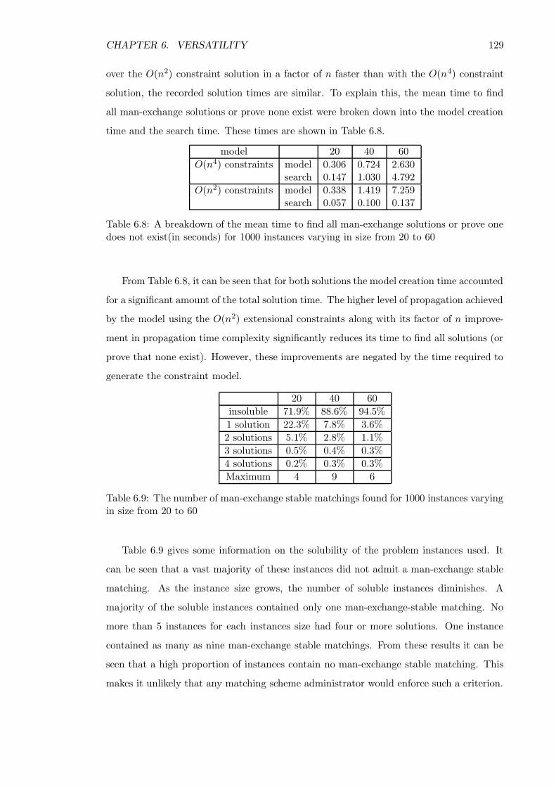
CHAPTER 6. VERSATILITY 129
over the O(n2) constraint solution in a factor of n faster than with the O(n4) constraint
solution, the recorded solution times are similar. To explain this, the mean time to find
all man-exchange solutions or prove none exist were broken down into the model creation
time and the search time. These times are shown in Table 6.8.
model 20 40 60
O(n4) constraints model 0.306 0.724 2.630search 0.147 1.030 4.792
O(n2) constraints model 0.338 1.419 7.259search 0.057 0.100 0.137
Table 6.8: A breakdown of the mean time to find all man-exchange solutions or prove onedoes not exist(in seconds) for 1000 instances varying in size from 20 to 60
From Table 6.8, it can be seen that for both solutions the model creation time accounted
for a significant amount of the total solution time. The higher level of propagation achieved
by the model using the O(n2) extensional constraints along with its factor of n improve-
ment in propagation time complexity significantly reduces its time to find all solutions (or
prove that none exist). However, these improvements are negated by the time required to
generate the constraint model.
20 40 60
insoluble 71.9% 88.6% 94.5%
1 solution 22.3% 7.8% 3.6%
2 solutions 5.1% 2.8% 1.1%
3 solutions 0.5% 0.4% 0.3%
4 solutions 0.2% 0.3% 0.3%
Maximum 4 9 6
Table 6.9: The number of man-exchange stable matchings found for 1000 instances varyingin size from 20 to 60
Table 6.9 gives some information on the solubility of the problem instances used. It
can be seen that a vast majority of these instances did not admit a man-exchange stable
matching. As the instance size grows, the number of soluble instances diminishes. A
majority of the soluble instances contained only one man-exchange-stable matching. No
more than 5 instances for each instances size had four or more solutions. One instance
contained as many as nine man-exchange stable matchings. From these results it can be
seen that a high proportion of instances contain no man-exchange stable matching. This
makes it unlikely that any matching scheme administrator would enforce such a criterion.

CHAPTER 6. VERSATILITY 130
However, it may be desirable to find a matching in which the number of pairs of men that
are not man-exchange stable is minimised.
6.4 Stable roommates
6.4.1 The problem
The Stable Roommates problem (SR) is a generalisation of the Stable Marriage problem
in which a group of n individuals wish to be matched into pairs. For convenience, it is
assumed that n is an even number. Each individual has a preference list in which all the
others are ranked in strict order. The objective of the problem is to find a matching that is
stable, where the definition of stability, in this case, is similar to the definition of stability
in the context of the stable marriage problem. This problem has been described in detail
in Section 2.3.
6.4.2 Constraint solution
The SM2 constraint, detailed in Section 3.2, ensures that the constrained pair do not form
a blocking pair or be assigned values that violate the matching, meaning that it ensures
that either they are matched to each other or are both matched to different people. As the
definition of stability for the Stable Roommates problem is similar to that for the Stable
Marriage problem, an instance of SR can be modelled by posting an SM2 constraint for
each pair of participants that appear in each other’s preference list. SR can also be mod-
elled using the SMN constraint that was detailed in Section 3.3. Each participant will be
represented by a single constrained integer variable, with domain values representing pref-
erences. The constraint will then be set up such that the variable representing participant
ri will go in place of the variables representing both mi and wi. Similarly, ri’s preference
list will be copied in place of both mi and wi’s preference lists. During propagation, vari-
able zi and variable zn+i will be the same variable, meaning that any value removed from
dom(zi) will also be removed from dom(zn+i). When the SMN constraint is used to find
stable matchings in a Stable Marriage instance, it is the case that removing a value from
a male variable can only cause propagation to occur to a female variable. When SMN
is used to solve a stable roommates instance, this is no longer the case; as a result some
proofs presented in Chapter 3 will not carry over to the SR case. As a result, enforcing
arc-consistency will no longer be sufficient to find a solution, neither can it be guaranteed

CHAPTER 6. VERSATILITY 131
that all solutions can be found in a failure free search. However, this constraint can be
used to find all stable matchings (or prove that none exist) for any given stable roommates
instance.
6.4.3 Empirical study
Both the SM2 and SMN solutions were implemented and used to solve randomly gener-
ated stable roommates instances (produced by the random instance generator detailed in
Appendix B.5). The instance sizes ranged from 200 to 1000 with 100 instances per value
of n.
model 200 400 600 800 1000
SM2 first solution Min 0.497 1.007 2.060 3.701 5.941Mean 0.543 1.194 2.557 4.729 7.779Max 0.596 1.421 3.021 5.490 9.433
all solutions Min 0.519 1.133 2.353 4.414 7.534Mean 0.564 1.260 2.725 5.016 8.170Max 0.615 1.385 3.013 5.511 9.230
SMN first solution Min 0.360 0.450 0.630 0.893 1.342Mean 0.377 0.471 0.664 0.947 1.416Max 0.421 0.490 0.694 1.009 1.468
all solutions Min 0.368 0.470 0.665 0.928 1.402Mean 0.383 0.479 0.674 0.963 1.432Max 0.421 0.490 0.689 1.009 1.455
Table 6.10: Time to find the first solution (or prove one does not exist) and all solutionsfor the Stable Roommates problem (in seconds) for 100 instances varying in size from 200to 1000
From Table 6.10, it can be seen that, finding a stable matching for a stable roommates
instance (or proving the instance insoluble) with these constraint solutions can be achieved
in similar time to a stable marriage instance with the equivalent number of participants2.
200 400 600 800 1000
% of insoluble instances 44 54 54 55 64mean number of solutions 2.642 3.434 3.586 3.733 4.75
maximum number of solutions 8 16 12 24 36
Table 6.11: Solubility results for the Stable Roommates problem for 100 instances varyingin size from 200 to 1000
From Table 6.11, it can be seen that as n increases the percentage of insoluble instances
2Note that a stable roommates instance has n participants and a stable marriage instance contains 2n
participants
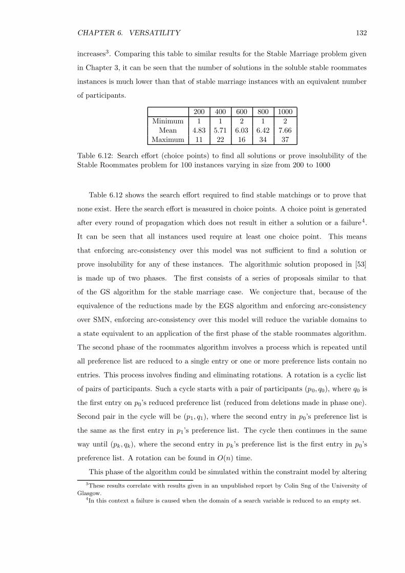
CHAPTER 6. VERSATILITY 132
increases3. Comparing this table to similar results for the Stable Marriage problem given
in Chapter 3, it can be seen that the number of solutions in the soluble stable roommates
instances is much lower than that of stable marriage instances with an equivalent number
of participants.
200 400 600 800 1000
Minimum 1 1 2 1 2Mean 4.83 5.71 6.03 6.42 7.66
Maximum 11 22 16 34 37
Table 6.12: Search effort (choice points) to find all solutions or prove insolubility of theStable Roommates problem for 100 instances varying in size from 200 to 1000
Table 6.12 shows the search effort required to find stable matchings or to prove that
none exist. Here the search effort is measured in choice points. A choice point is generated
after every round of propagation which does not result in either a solution or a failure4.
It can be seen that all instances used require at least one choice point. This means
that enforcing arc-consistency over this model was not sufficient to find a solution or
prove insolubility for any of these instances. The algorithmic solution proposed in [53]
is made up of two phases. The first consists of a series of proposals similar to that
of the GS algorithm for the stable marriage case. We conjecture that, because of the
equivalence of the reductions made by the EGS algorithm and enforcing arc-consistency
over SMN, enforcing arc-consistency over this model will reduce the variable domains to
a state equivalent to an application of the first phase of the stable roommates algorithm.
The second phase of the roommates algorithm involves a process which is repeated until
all preference list are reduced to a single entry or one or more preference lists contain no
entries. This process involves finding and eliminating rotations. A rotation is a cyclic list
of pairs of participants. Such a cycle starts with a pair of participants (p0, q0), where q0 is
the first entry on p0’s reduced preference list (reduced from deletions made in phase one).
Second pair in the cycle will be (p1, q1), where the second entry in p0’s preference list is
the same as the first entry in p1’s preference list. The cycle then continues in the same
way until (pk, qk), where the second entry in pk’s preference list is the first entry in p0’s
preference list. A rotation can be found in O(n) time.
This phase of the algorithm could be simulated within the constraint model by altering
3These results correlate with results given in an unpublished report by Colin Sng of the University ofGlasgow.
4In this context a failure is caused when the domain of a search variable is reduced to an empty set.
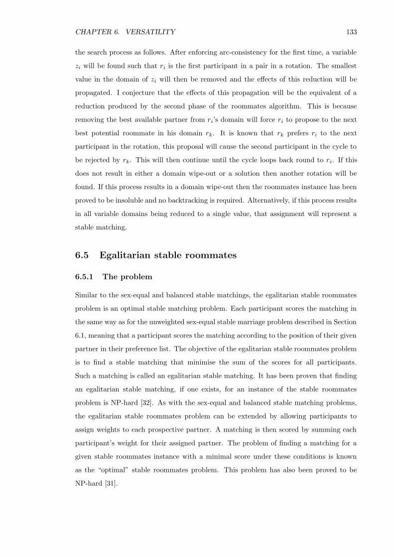
CHAPTER 6. VERSATILITY 133
the search process as follows. After enforcing arc-consistency for the first time, a variable
zi will be found such that ri is the first participant in a pair in a rotation. The smallest
value in the domain of zi will then be removed and the effects of this reduction will be
propagated. I conjecture that the effects of this propagation will be the equivalent of a
reduction produced by the second phase of the roommates algorithm. This is because
removing the best available partner from ri’s domain will force ri to propose to the next
best potential roommate in his domain rk. It is known that rk prefers ri to the next
participant in the rotation, this proposal will cause the second participant in the cycle to
be rejected by rk. This will then continue until the cycle loops back round to ri. If this
does not result in either a domain wipe-out or a solution then another rotation will be
found. If this process results in a domain wipe-out then the roommates instance has been
proved to be insoluble and no backtracking is required. Alternatively, if this process results
in all variable domains being reduced to a single value, that assignment will represent a
stable matching.
6.5 Egalitarian stable roommates
6.5.1 The problem
Similar to the sex-equal and balanced stable matchings, the egalitarian stable roommates
problem is an optimal stable matching problem. Each participant scores the matching in
the same way as for the unweighted sex-equal stable marriage problem described in Section
6.1, meaning that a participant scores the matching according to the position of their given
partner in their preference list. The objective of the egalitarian stable roommates problem
is to find a stable matching that minimise the sum of the scores for all participants.
Such a matching is called an egalitarian stable matching. It has been proven that finding
an egalitarian stable matching, if one exists, for an instance of the stable roommates
problem is NP-hard [32]. As with the sex-equal and balanced stable matching problems,
the egalitarian stable roommates problem can be extended by allowing participants to
assign weights to each prospective partner. A matching is then scored by summing each
participant’s weight for their assigned partner. The problem of finding a matching for a
given stable roommates instance with a minimal score under these conditions is known
as the “optimal” stable roommates problem. This problem has also been proved to be
NP-hard [31].
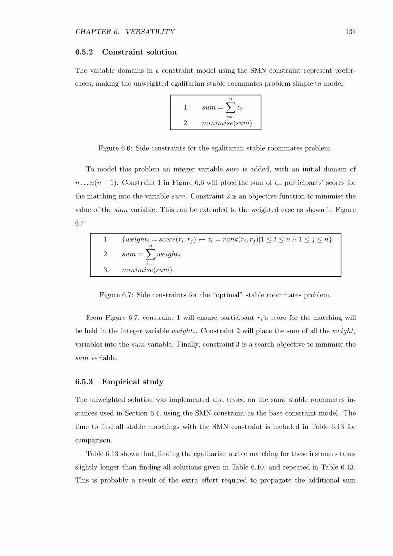
CHAPTER 6. VERSATILITY 134
6.5.2 Constraint solution
The variable domains in a constraint model using the SMN constraint represent prefer-
ences, making the unweighted egalitarian stable roommates problem simple to model.
1. sum =
n∑
i=1
zi
2. minimise(sum)
Figure 6.6: Side constraints for the egalitarian stable roommates problem.
To model this problem an integer variable sum is added, with an initial domain of
n . . . n(n − 1). Constraint 1 in Figure 6.6 will place the sum of all participants’ scores for
the matching into the variable sum. Constraint 2 is an objective function to minimise the
value of the sum variable. This can be extended to the weighted case as shown in Figure
6.7
1. weighti = score(ri, rj) ↔ zi = rank(ri, rj)|1 ≤ i ≤ n ∧ 1 ≤ j ≤ n
2. sum =
n∑
i=1
weighti
3. minimise(sum)
Figure 6.7: Side constraints for the “optimal” stable roommates problem.
From Figure 6.7, constraint 1 will ensure participant ri’s score for the matching will
be held in the integer variable weighti. Constraint 2 will place the sum of all the weighti
variables into the sum variable. Finally, constraint 3 is a search objective to minimise the
sum variable.
6.5.3 Empirical study
The unweighted solution was implemented and tested on the same stable roommates in-
stances used in Section 6.4, using the SMN constraint as the base constraint model. The
time to find all stable matchings with the SMN constraint is included in Table 6.13 for
comparison.
Table 6.13 shows that, finding the egalitarian stable matching for these instances takes
slightly longer than finding all solutions given in Table 6.10, and repeated in Table 6.13.
This is probably a result of the extra effort required to propagate the additional sum

CHAPTER 6. VERSATILITY 135
200 400 600 800 1000
all solutions Min 0.368 0.470 0.665 0.928 1.402Mean 0.383 0.479 0.674 0.963 1.432Max 0.421 0.490 0.689 1.009 1.455
egalitarian solution Min 0.391 0.507 0.704 1.003 1.417Mean 0.399 0.522 0.722 1.036 1.474Max 0.449 0.539 0.746 1.117 1.526
Table 6.13: The mean time to find an egalitarian solution (if one exists) for the stableroom mates problem (in seconds) for 100 instances varying in size from 200 to 1000
constraint. Usually, finding an optimal solution requires less effort than finding all solutions
despite the extra overhead required to propagate the optimisation value. This is because
the full search tree need not be explored due to extra propagation from the optimisation
function. This is not the case here. This is probably a result of both the very low number
of solutions in the problem instances as shown in Table 6.11 and the poor propagation
delivered by the sum constraint.
6.6 Forbidden pairs
6.6.1 The problem
An administrator of a matching scheme may wish to ensure that a particular pair are
not matched to one another in a given stable matching. This pair may still find each
other acceptable and thus they could still form a blocking pair; for this reason, we cannot
delete this pair from each other’s preference lists. Such a (man,woman) pair is known as
a forbidden pair [30].
Let F denote the set of forbidden pairs. A stable matching M is a valid solution to the
stable marriage problem with forbidden pairs iff ∀(mi, wj) ∈ F, (mi, wj) /∈ M . A linear
time algorithm has been published to find such a matching for the stable marriage case, if
one exists [30]. However, when including forbidden pairs, a stable matching may not exist
for a given stable matching instance. For such an instance, it may be desirable to relax
the requirement that the matching contain no forbidden pairs. It could be advantageous
to find a matching that contains the fewest number of forbidden pairs. For the stable
marriage case, such a matching can be found in polynomial time [33].

CHAPTER 6. VERSATILITY 136
6.6.2 Constraint solution
Constraint models are now given for the Stable Marriage problem with Forbidden Pairs.
These solutions can be adapted for the Stable Roommates and Hospitals/Residents cases.
This problem could be modelled by adding a unary constraint for each forbidden pair in
the set F , as follows:
1. zi 6= pref(i, j) ∀ij, (mi, wj) ∈ F
Figure 6.8: Side constraint for the Stable Marriage Problem with Forbidden Pairs.
A constraint model representing a stable marriage instance with forbidden pairs, will
require at most O(n2) of the constraints shown in Figure 6.8. Therefore, the space com-
plexity of the original model will not be increased. Each constraint can be propagated in
O(1) time and so the time complexity will not be affected either.
The optimisation version of the problem (to find a matching containing the fewest
number of forbidden pairs) could be modelled by adding an array of constrained integer
variables f each with an initial domain of 0, 1, for each forbidden pair. Such a variable
will be assigned the value 1 if the corresponding forbidden pair is included in the matching,
otherwise it will be assigned the value 0. A constrained integer variable sumF with an
initial domain of 0 . . . |F | would also be added to hold the sum of all the new f variables.
1. zi = pref(i, j) ⇔ fk > 0 1 ≤ k ≤ |F |,∀ij, (mi, wj) ∈ F
2. sumF =
|F |∑
k=1
fk
3. minimise(sumF )
Figure 6.9: Side constraints for the optimisation version of the Stable Marriage Problemwith Forbidden Pairs.
Constraint 1, from Figure 6.9, ensures that if a forbidden pair is in a matching then
the appropriate f variable is set to 1. Constraint 2 places the sum of the f variables
in the variable sumF . Finally, constraint 3 is an optimisation objective to minimise the
sumF variable5. This solution could also be easily extended to have a weight wp for each
forbidden pair f , thus, allowing the expression of a preference over which pairs are to be
excluded from the matching. This could be implemented by changing the initial domain
of f to 0,wp.
5This constraint model was proposed by Manlove et al. in [70]

CHAPTER 6. VERSATILITY 137
6.7 Forced pairs
6.7.1 The problem
As well as forbidding certain pairs from being matched to each other, an administrator of a
matching scheme may also wish to force a certain pair or set of pairs to be matched. Such
pairs are referred to as forced pairs [60]. Finding a stable matching under these conditions
can be found in linear time [30].
Let Q denote the set of forced pairs. A stable matching M is a valid solution to
the stable marriage problem with forced pairs iff ∀(mi, wj) ∈ Q, (mi, wj) ∈ M . Such a
matching need not exist. Thus, an optimisation version of the problem may be required
to find a matching with the largest number of forced pairs. Such a matching can be found
in polynomial time [33].
6.7.2 Constraint solution
One way to extend an SM constraint model to include this problem would be to have a
constraint for each forced pair, as shown in Figure 6.10.
1. zi = pref(i, j) ∀ij, (mi, wj) ∈ Q
Figure 6.10: Side constraint for the Stable Marriage Problem with Forced Pairs.
To model this as an optimisation problem, an array of constrained integer variables q
of length |Q| is added, each with an initial domain of 0, 1. A constrained integer variable
sumQ with an initial domain of 0 . . . |Q| would also be needed to hold the value of the
solutions.
1. zi = pref(i, j) ⇔ qk > 0 1 ≤ k ≤ |Q|,∀ij, (mi, wj) ∈ Q
2. sumQ =
|Q|∑
k=1
qk
3. maximise(sumQ)
Figure 6.11: Side constraints for the optimisation version of the Stable Marriage Problemwith Forced Pairs.
Constraint 1 from Figure 6.11 ensures that if a forced pair is in a matching then the
appropriate q variable is set to 1. Constraint 2 places the sum of all the q variables in the
variable sumQ. Finally, constraint 3 is an optimisation objective to maximise the sumQ

CHAPTER 6. VERSATILITY 138
variable. This solution could be extended to have a weight wp for each forced pair q, thus,
allowing the expression of a preference over which pairs get excluded from the matching.
This could be implemented by changing the initial domain of q to 0,wp.
6.8 Couples
6.8.1 The problem
An extension of the Hospitals/Residents problem is to allow couples to submit joint pref-
erence lists. This allows two residents to state that they would like to be assigned to
hospitals that are geographically close. This problem as described by Ronn [81] alters the
definition of stability of the original problem. Therefore, this problem cannot be modelled
by adding side constraints to an existing Hospitals/Residents constraint model. However,
there is a simplified version of this problem in which a set of couples C (each couple con-
sisting of two residents) wish to be assigned to the same hospital. In this version of the
problem, each resident in the couple can still form a blocking pair in the same way as
for the classical Hospitals/Residents problem. Under these restrictions, a stable matching
need not exist, which gives rise to the optimisation problem to find a stable matching in
which the largest number of couples are honoured.
Similar to the couples problem is the enemies problem, in which two residents request
to be assigned to different hospitals. Residents that appear in a pair of enemies may still
form a blocking pair in the usual way. Under these extra conditions, not all problem
instances will admit a consistent stable matching, giving rise to the optimisation version
of the problem. The objective of this problem is to find a matching in which the number
of enemies assigned to the same hospital is minimised.
6.8.2 Constraint solution
A simple way to model the couples problem would be to make the assumption that each
resident in a couple will submit a preference list which is identical to that of their partner
in the couple. By making this assumption, this problem can be modelled by a single
constraint for each couple.
1. xi = xk ∀ik, (ri, rk) ∈ C
Figure 6.12: Side constraint for the couples Hospitals/Residents problem.
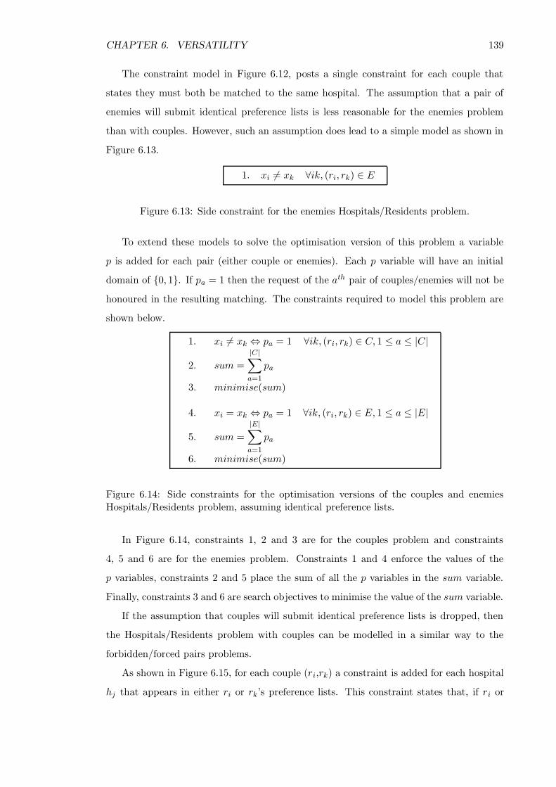
CHAPTER 6. VERSATILITY 139
The constraint model in Figure 6.12, posts a single constraint for each couple that
states they must both be matched to the same hospital. The assumption that a pair of
enemies will submit identical preference lists is less reasonable for the enemies problem
than with couples. However, such an assumption does lead to a simple model as shown in
Figure 6.13.
1. xi 6= xk ∀ik, (ri, rk) ∈ E
Figure 6.13: Side constraint for the enemies Hospitals/Residents problem.
To extend these models to solve the optimisation version of this problem a variable
p is added for each pair (either couple or enemies). Each p variable will have an initial
domain of 0, 1. If pa = 1 then the request of the ath pair of couples/enemies will not be
honoured in the resulting matching. The constraints required to model this problem are
shown below.
1. xi 6= xk ⇔ pa = 1 ∀ik, (ri, rk) ∈ C, 1 ≤ a ≤ |C|
2. sum =
|C|∑
a=1
pa
3. minimise(sum)
4. xi = xk ⇔ pa = 1 ∀ik, (ri, rk) ∈ E, 1 ≤ a ≤ |E|
5. sum =
|E|∑
a=1
pa
6. minimise(sum)
Figure 6.14: Side constraints for the optimisation versions of the couples and enemiesHospitals/Residents problem, assuming identical preference lists.
In Figure 6.14, constraints 1, 2 and 3 are for the couples problem and constraints
4, 5 and 6 are for the enemies problem. Constraints 1 and 4 enforce the values of the
p variables, constraints 2 and 5 place the sum of all the p variables in the sum variable.
Finally, constraints 3 and 6 are search objectives to minimise the value of the sum variable.
If the assumption that couples will submit identical preference lists is dropped, then
the Hospitals/Residents problem with couples can be modelled in a similar way to the
forbidden/forced pairs problems.
As shown in Figure 6.15, for each couple (ri,rk) a constraint is added for each hospital
hj that appears in either ri or rk’s preference lists. This constraint states that, if ri or

CHAPTER 6. VERSATILITY 140
1. xi = pref(i, j) ⇔ xk = pref(k, j) ∀ikj, (ri, rk) ∈ C, j ∈ PL(i) ∪ PL(k)
Figure 6.15: Side constraint for the couples Hospitals/Residents problem.
rk is matched to hj then the other must also be matched to the same hospital. It is
assumed that if j /∈ PL(k) then pref(k, j) will return −1. The effect of this is that if ri
were matched to a hospital that does not appear in rk’s preference list then the constraint
would remove all values from the domain of xk except the value −1, this will cause a failure
and trigger a backtrack. To modify this model for the enemies problem, = is replaced with
6=.
Both the couples and enemies problems can also be modelled with extensional con-
straints.
1. Ci,k =
(a, b)|j ∈ PL(i), j ∈ PL(k),a = rank(ri, wj) ∧ b = rank(rk, wj)
Figure 6.16: Extensional constraint for the couples Hospitals/Residents problem.
The extensional constraint model for the couples problem shown in Figure 6.16 posts
an extensional constraint for each couple (ri,rk) which contains the set of allowed tuples
representing the two residents being matched to the same hospital. A pair (a, b) is a valid
assignment, with respect to the constraint Ci,k, for the pair of variables representing ri
and rk respectively, if a represents ri’s preference for some hospital hj and b represents
rk’s preference for the same hospital hj .
1. Ci,k =
(a, b)|j ∈ PL(i), l ∈ PL(k), j 6= l,a = rank(ri, wj) ∧ b = rank(rk, wl)
Figure 6.17: Extensional constraint for the enemies Hospitals/Residents problem.
As shown in Figure 6.17, a pair (a, b) is a valid assignment, with respect to the con-
straint Ci,k, for the pair of variables representing ri and rk respectively, if a represents a
hospital hj in ri’s domain and b represents a hospital hl in rk’s domain and hj 6= hl. These
extensional constraint models can then be extended to solve the optimisation version of
the respective problems as shown below.
In the constraint model in Figure 6.18, Ci,k refers to the extensional constraint for the
couples Hospitals/Residents problem as detailed in Figure 6.16. Constraint 1 states that

CHAPTER 6. VERSATILITY 141
1. Ci,k ⇔ pa = 1 ∀ik, (ri, rk) ∈ C, 1 ≤ a ≤ |C|
2. sum =
|C|∑
i=1
cpi
3. minimise(sum)
Figure 6.18: Extensional constraint for the optimisation version of the couples Hospi-tals/Residents problem.
either the ith couple is included in the matching or the variable pi is assigned the value 1.
Constraint 2 places the sum of all the p variables into the sum variable. Finally, constraint
3 is an optimisation function to minimise the value held in the sum variable. To adapt
this model for the enemies Hospitals/Residents problem, the extensional constraint in line
1 is changed to the one described in Figure 6.17.
6.9 Conclusions
In this chapter it has been shown that adding simple side constraints to the specialised
constraint models proposed in Chapters 3 and 5 can model several extensions of classical
stable matching problems. However, the true versatility of these solutions does not become
apparent until a problem in which many of the above extensions are mixed together needs
to be modelled. For example, there could be a Hospitals/Residents instance I in which
a pair of residents r2 and r7 are good friends, and if they find that they would rather
have each other’s assigned hospital than their own then they will complain. To avoid this
a man-exchange stability constraint is posted over their two variables. Another pair of
residents r3 and r9 are married and wish to be assigned to the same hospital, so a couples
constraint is posted to enforce this. A doctor at hospital h5 has requested that his son,
resident r4, not be assigned to his hospital, so a forbidden pair constraint is posted to
enforce this. A teacher thinks that residents r1, r5 and r12 are too dependent on each
other’s help and would like to split them up, so a clique of enemy constraints is posted
to enforce this. Along with all these extra conditions the most balanced matching6 is
required so an objective function is posted to find it. These, or any other similar set of
constraints, can simply be added to any of the specialised constraints without the need
to alter the base model, but will allow for very rich problems to be easily modelled and
6The definition of a balanced matching in the Hospitals/Residents case is not clear, it is used here forillustrative purposes only
CHAPTER 6. VERSATILITY 142
solved (or to prove that no solution exists).
As has been shown in this Chapter, constraint technologies can provide very versatile
solutions to stable matching problems. Furthermore, it can also allow for rapidly mod-
elling hard combinatorial problems for which no algorithmic solutions currently exists.
This allows such problems to be empirically studied to provide insights into the problems
structure.
6.10 Future work
In the experiments done in this chapter, the value ordering heuristic used was not altered
from that used by the original specialised constraints to find all stable matchings. That
variable ordering heuristic is to choose the variable with the smallest minimum domain
value and the value ordering heuristic was to choose the smallest domain value first. This
is used in the all solutions case because it results in a failure free search process (as
shown in Chapter 3). It may be the case that, for a problem in which we seek a specific
optimal matching (under some definition of optimality) a different set of variable and
value ordering heuristics may lead to finding such an optimal solution more efficiently.
For example, one possible value ordering that may work well for the sex-equal stable
marriage problem would be to choose a value that is the most equal locally. For example,
when choosing a value to try for variable zi, find the value that minimises the difference
between mi’s preference from the chosen woman and the woman’s preference for him.
More formally, choose woman wj such that |rank(mi, wj) − rank(wj,mi)| is minimised.
Alternatively a dynamic value ordering could monitor the current states of the summ
and sumw variables and choose a value that will help to unify them. Similarly for the
balanced stable marriage problem when selecting a value from the domain of zi, choose
woman wj such that maxrank(mi, wj), rank(wj ,mi) will be minimised. Or a dynamic
value ordering could monitor the current states of the summ and sumw variables and
choose a value that will help to minimise the largest of them. Possible variable ordering
heuristics include choose the variable with the largest current domain; this should cause the
maximum propagation and thus reduce the search tree. Conversely, choosing the variable
with the smallest domain may be advantageous for problems with a high probability of
insolubility, as it may result in empty domains more quickly.

Chapter 7
Conclusion and future work
7.1 Conclusion
In Chapter 2 a number of constraint solutions for stable matching problems have been
detailed. The justification for these constraint solutions has always been the inherent
versatility of the generalised framework within which the constraint solutions are based.
However, this versatility was not demonstrated. Empirical comparison has shown that
none of these solutions come close to the runtime performance of the specialised algorithmic
solutions for these problems.
My contribution to the field starts in Chapter 3, which demonstrates how the stable
marriage problem can be modelled as a specialised constraint. Two specialised constraints
were presented; a binary constraint SM2 and an n-ary constraint SMN. Proofs have been
given which state that when propagated the SMN constraint reduces the variable domains
to a state which is the equivalent of the GS-lists. Furthermore, this can be achieved in
O(n2) time (which is optimal in the size of the preference lists). Therefore, propagating the
SMN constraint is sufficient to find a stable matching without search. Further proofs state
that, by using a simple value ordering all stable matchings can be enumerated without
failure due to an incorrect assignment. Empirical evidence has been presented which
shows that these specialised constraint solutions can solve problem instances significantly
faster than previously published constraint models. It can be seen that for large instances
where n = 8000 the SMN constraint is within a factor of four of the specialised algorithmic
solution’s runtime. This is achieved whilst maintaining the full versatility of the constraint
satisfaction problem architecture.
In Chapter 4 two further specialisations of the n-ary stable marriage constraint were
143
CHAPTER 7. CONCLUSION AND FUTURE WORK 144
presented. These specialisations reduce either the memory requirements to store or to
propagate the constraint. Empirical evidence was given which shows the benefits of these
improvements. The first constraint reduced the time to enforce arc-consistency and the
second constraint reduced the time to find all solutions. However, these benefits come at
the cost of versatility.
In Chapter 5 it was shown how the Hospitals/Residents problem can be modelled
as a specialised constraint. Empirical evidence was presented which showed that this
solution can solve problem instances significantly faster than a toolbox constraint model.
Furthermore, it has been shown that the specialised constraint can solve problem instances
of a size equivalent to that of the “real life” Hospitals/Residents problems.
Finally, Chapter 6 demonstrated the versatility of the constraint solutions presented
in Chapters 3 and 5. This was done by adding side constraints to the existing specialised
constraint models to model a number of different sub-problems. These problems either
gave a definition of optimality or restricted the set of solutions by adding additional cri-
teria. Many of these problems have been proven to be NP-Hard and some have no known
algorithmic solutions. Included with these models are the results from empirical studies
which show that these are indeed feasible solutions to these problems. These studies also
provide some insight into the structure of these problems, some of which have had little
or no previous study.
7.2 Future work
7.2.1 Enforcing GAC over SMN
In Chapter 3 a specialised n-ary constraint (SMN) for the stable marriage problem is
presented. Unlike most n-ary constraints SMN enforces arc-consistency (AC), rather than
generalised arc-consistency (GAC), which is the usual level of consistency enforced over
such a constraint. The reason for this is that enforcing AC in this case is sufficient to find
a stable matching. Maintaining this level of consistency is also sufficient to enumerate all
stable matchings in a failure free search process. Therefore, enforcing a higher level of
consistency will not reduce the size of the search tree.
However, if enforcing GAC was desirable for this constraint then one way this could
be achieved would be by emulating the algorithm proposed by Gusfield [48] for finding
the set of all stable pairs. A pair is said to be a stable pair iff it appears in at least

CHAPTER 7. CONCLUSION AND FUTURE WORK 145
one stable matching. The SMN constraint represents a whole stable marriage instance;
enforcing GAC over this constraint will mean that all values remaining after propagation
must appear in a valid n-tuple, meaning it must appear in a stable matching. Therefore,
enforcing GAC over this constraint is the equivalent of finding all stable pairs.
The algorithm proposed by Gusfield [48] for this problem exploits the lattice structure
of the stable marriage problem. The algorithm starts by finding both the male-optimal and
female-optimal stable matchings. It then uses a procedure called “breakmarriage” which
takes an arbitrary man mi, such that mi has a different partner in the two matchings, and
denies him his first choice partner. mi is then placed on the free list. The GS algorithm [36]
is then restarted. This is then repeated until the GS algorithm returns only one matching.
It has been proven [48] that all stable pairs will be included in at least one of the matchings
returned by this process. This algorithm has been shown to run in O(n2) time.
After propagating the SMN constraint, if an arbitrary uninstantiated man variable zi
has its lowest domain value removed and the effects are propagated, the resultant domain
reductions will be the equivalent of running the “breakmarriage” procedure. This is then
repeated until all variables are instantiated. The stable pairs will be recorded and the state
of the variable domains will be returned to that after the initial propagation call. Any
domain value that does not appear in a stable pair will then be removed. The remaining
domain values will then be GAC. During this process Θ(n2) domain values will be removed,
each value will require O(1) time to propagate, thus this method will run in Θ(n2) time
(assuming the backtrack can be achieved within the same time complexity).
It would be sufficient to implement this method as part of the init method of the SMN
constraint and use the same remV al method as the AC version to maintain consistency.
This would mean that this method need only be called once. Using this method, GAC
can be enforced with same worst case time complexity as enforcing AC. However, the best
case complexity of enforcing AC is significantly better. It is doubtful that the benefits
gained by enforcing this higher level of consistency would outweigh the effort required to
enforce it, but this has not yet been empirically tested.
7.2.2 Value and variable ordering heuristics
For the stable marriage problem, it has been shown that, using a value ordering heuristic
of choosing the favourite partner remaining in the domain with an arbitrary variable
ordering heuristic, is sufficient to find all stable matchings without backtracking due to a
CHAPTER 7. CONCLUSION AND FUTURE WORK 146
bad branching decision. The same is also true in the Hospitals/Residents case. However,
when the objective is shifted to finding some form of optimal matching a different set of
heuristics may be more appropriate.
7.2.3 Allowing indifference
A common generalisation of a stable matching problem is to allow ties in the preference
list. By allowing ties in a preference list, participants have the ability to express indiffer-
ence between two or more potential partners. Some provisional work has been conducted
into developing specialised constraints for stable matching problems with ties [92]. This
work includes showing how a stable matching problem with ties can be represented within
a specialised constraint such that all required ties information can be accessed in con-
stant time. Provisional results of attempting to find the maximal stable matching using
anonymised data from SFAS [56] have shown that this is not a viable solution for these
problem instances, in its current form. It may be the case that better value and variable
ordering heuristics may improve this.
An alternative solution would be to reformulate the problem as a permutation problem.
It is known that under weak stability a stable matching can be found by arbitrarily breaking
the ties and solving the resulting instance in the same way as the no ties case. When no
ties are present in an instance all stable matchings are of the same size. Therefore, the
problem could be reformulated from trying to find an optimal matching to trying to find
an optimal permutation of the preference lists.
In 2002, Gent and Prosser [44] proposed a constraint model to solve the stable marriage
problem with ties and incomplete preference lists. The authors presented empirical results
obtained by using this model to solve randomly generated problem instances. This was
then used to solve problem instances generated with a fixed probability of incompleteness
while varying the probability of ties from 0 to 11. This was done in an attempt to observe
a phase transition as the problem changes from easy (with no ties) to hard (some ties)
and back to easy again (complete indifference). However, this phase transition was not
observed. It was suggested that this may be due to the relatively small instances used
(n = 10). It would be interesting to repeat these experiments with a larger instance size
to see if the phase transition can be seen. Another possible reason for the phase transition
not being observed was due to the random instance generator (detailed in Appendix B.3)
1In this case, probability of ties means the probability of any given preference list entry being tied withthe next entry on the list.

CHAPTER 7. CONCLUSION AND FUTURE WORK 147
that they used. This generator favours instances with many short ties. Instances with few
long ties will probably be much harder to solve. For this reason, the phase transition may
be observed if the experiments were repeated using a random instance generator designed
to produce instances with few long ties, such as the one proposed in Appendix B.4.
7.2.4 A compact bound stable marriage constraint
Two specialisations of the SMN constraint were given in Chapter 4. In one, only domain
reductions that affect the bounds of the variable were allowed. The other represented a
problem instance with a single set of n variables. The former showed a reduction in the
time to enforce arc-consistency (and thus find the first matching). The latter reduced
the time to enumerate all solutions. It would be interesting to see how a constraint
which combined these two ideas would perform. However, such a constraint would not be
very useful as its compact variable representation and reduced propagation would greatly
restrict its versatility.
7.2.5 Bound Hospitals/Residents constraint
In Chapter 4 it was shown that reducing the memory requirements of the SMN constraint
by not removing internal domain values resulted in a faster propagating constraint. A
similar modification could be developed for the Hospitals/Residents constraint. The com-
plication with this idea is that the HRN constraint as proposed in Chapter 5 represents
each hospital with a single variable. If interior domain reductions were disallowed then
another method of keeping track of each hospital’s c favourite residents would have to be
developed, since this is normally achieved via the hospital variable’s domain. This problem
could be addressed by having a separate variable for each post at each hospital, but the
additional variables may outweigh the benefits gained. Another solution could be to only
allow a domain reduction if it is a bound or one of the lowest c values in the domain of a
hospital variable. Alternatively, this information could be stored within a specialised data
structure made up of reversible variables.
7.2.6 Specialised constraints for other variants
of stable matching problems
An avenue for future research would be to develop specialised constraints for other stable
matching problems. One such class of problems is matching three or more sets of par-

CHAPTER 7. CONCLUSION AND FUTURE WORK 148
ticipants such as the 3-way or 3D stable matching problem [75]. It is NP-Complete to
determine if a stable matching exists in a given instance, thus a constraint approach may
be a viable solution for this problem.
In Chapter 6 a simplification of the stable couples problem was shown that can be
solved by adding side constraints to the specialised Hospitals/Residents constraint. How-
ever, the original version of this problem [81] alters the definition of stability and thus
cannot be solved by adding side constraints to an existing model. A specialised constraint
may be able to represent this version of the problem as a standalone constraint. Alterna-
tively, adding an additional method and/or auxiliary functions to the existing specialised
Hospitals/Residents constraint could allow for a mix of couples and singles in the same
problem.
In Chapter 6 it was shown how the man-exchange stable marriage problem can be
modelled by adding simple side constraints. Both solutions proposed have large memory
requirements which have a significant impact on the runtime of the solutions. A specialised
constraint solution could be developed to represent this problem in a more memory efficient
manner.
Not all stable roommates instances contain a stable matching. For an insoluble in-
stance, it may be desirable to find a matching that is “Almost Stable” [8]. An “Almost
Stable” matching is a matching which contains the fewest number of blocking pairs over all
matchings. This problem could probably be modelled by using a stripped down version of
the SMN constraint, which only enforces that returned solutions constitute a valid match-
ing. A boolean variable could then be added for each man which holds the number of
blocking pairs that man is involved with. This could probably be enforced with a stripped
down version of the SM2 constraint which only enforces stability in conjunction with a
disjunctive statement that says if mi forms a blocking pair with wj then increment some
counter.

Appendix A
Glossary
A.1 Terms and definitions
In this appendix a number of terms are defined that are used throughout this dissertation.
• Constraint Solver : A library of tools that can be used to model and solve con-
straint satisfaction problems. It is assumed that this constraint solver uses an AC5-
like framework [96].
• Constrained Integer Variable : An object which is supplied by the constraint
solver to represent an integer variable within a constraint satisfaction problem. Each
variable has an associated finite integer domain. If at any point during search the
domain of a constrained integer variable is reduced to an empty set then the current
search node will be marked as a fail and a backtrack will be forced. The solver will
track the values in each variable’s domain and on backtracking the domains will be
returned to their previous state.
• Search variable / non-search variable : Each constraint model has a set of
search variables. A solution to that constraint model consists of a mapping of domain
values to search variables. Therefore, to find a solution the constraint solver will first
propagate the constraints. If that does not result in either a failure or a solution,
then the solver will choose one of the search variables that is not yet instantiated and
branch over that variable. This will then be repeated until all the search variables
are instantiated. A non-search variable works in the same way as a search variable
except that it does not have to be instantiated for a solution to be found. However
149

APPENDIX A. GLOSSARY 150
if a non-search variable has its domain reduced to an empty set then it will cause a
failure to be reported and a backtrack will occur.
• Reversible Integer Variable : An object which is supplied by the constraint
solver to store an integer value within a constraint. The values of these variables
will be stored by the solver and restored on backtracking.
• Toolbox Constraints : A set of constraints supplied by the constraint solver to
construct constraint models. Such constraints usually consist mainly of standard
mathematical and logical operators.
• Global constraint : Bessiere et al. [19] defined a global constraint GC to be a
constraint which cannot be decomposed into a set of lesser arity constraints CS,
such that the propagation achieved by GC is greater than CS or the time and space
complexity of GC to achieve this propagation is lower than that of CS. In this
dissertation the term global constraint is used to mean a constraint with an arity n
where n is a parameter.
• Specialised constraint : A specialised constraint is a constraint that has been
written to solve a specific problem or sub problem. For example, the flow constraint
[23] written to help model the network flow problem.
• Side constraints : A side constraint is a constraint that has been added to an
existing constraint model. These are normally used either to increase propagation to
make the model more efficient, or to restrict the set of solutions in some way to solve
some restricted version of the problem the original model was designed to solve.
A.2 Objects and functions
The following is a list of the objects and functions used in the pseudo-code throughout
this thesis.
• dom(z) : Returns the current set of values that make up the domain associated with
the variable z.
• max(dom(z)) : Returns the largest value in the domain of variable z.
• min(dom(z)) : Returns the smallest value in the domain of variable z.

APPENDIX A. GLOSSARY 151
• isInstantiated(dom(z)) : returns true iff |dom(z)| = 1
• getNextHigher(dom(z), a) : Returns the smallest value in the domain of variable z
that is strictly greater than the value a, if no such value exists then this procedure
returns a.
• getV alue(dom(z), a) : Returns the ath smallest value in dom(z), if |dom(z)| < a
then it returns max(dom(z)).
• delV al(dom(z), a) : Removes the value a from the domain of variable z.
• delRange(dom(z), a, b) : Removes all values v from the domain of variable z such
that a ≤ v ≤ b. Note that if a > b then no values will be removed.
• setMax(dom(z), a) : Removes all values strictly greater than a from the domain of
variable z.
• PL(i, a) : Returns the integer index of the ath person in the ith person’s preference
list.
• rank(mi, wj) : Returns the position of wj in mi’s preference list.
• pref(i, j) : Returns the position of the j th participant in the ith participants prefer-
ence list. This function is similar to rank(mi, wj). The difference between the two
is the context in which they are used. In general pref(i, j) is used in pseudo-code
while rank(mi, wj) is used in text. pref(i, j) is assumed to be implemented (unless
stated otherwise) by means of an inverse preference list. For the Stable Marriage
problem the inverse preference lists are modelled as a pair of two dimensional integer
arrays. Note that the inverse preference lists can be constructed in O(n2) time since
the preference lists are being read by making pref(i, j) = k where PL(i, k) = j.
• lmi : the length of mi’s preference list.
• swap(x, y) : Swaps the values of the integer variables x and y.

Appendix B
Problem generators
In this appendix details are presented about the problem instance generators used to
generate the random instances used in the empirical studies throughout this thesis. These
instance generators will be given in a Java-like pseudo-code, using the . (Dot) operator as
an attribute selector. For example, A.b() will indicate a call to the method b() associated
with the object A. Two predefined object classes will be used in this appendix arrayList
and randomInt. An arrayList x is an ordered variable length array indexed from 1, with
three associated methods as follows.
• x.init(a, b) will initialise the arrayList x by adding an integer i to x for each integer
in the range a ≤ i ≤ b.
• x.add(a) will add the object a to the arrayList x, and thus increment the length of
x by one.
• x.remove(i) will return the ith object from the arrayList x, this object will also be
removed from the arrayList x and thus the length of x is decremented by one.
• x.lookUp(i) will return the index of i in the arrayList x. If i /∈ x then −1 is returned.
• x.length will return the current number of objects held in the arrayList x.
The object random is a pseudo-random number generator with two associated methods
as follows.
• x.init(seed) will initialise the random object x with the integer seed value seed.
Storing the seed value used along with the instance generator for a set of instances
152

APPENDIX B. PROBLEM GENERATORS 153
will allow the instances to be reproduced if necessary without having to store them
as a number of potentially large text files.
• x.nextInt(y, z) will return an integer i arbitrarily picked from the range y ≤ i ≤ z.
• x.nextReal(y, z) will return a real number i arbitrarily picked from the range y ≤
i ≤ z.
It is also assume that there is access to a method named write(a) which will output
the arguments to a text file in some standard format.
B.1 Stable marriage instance generator
The stable marriage instance generator produces a complete set of n male preference lists
and n female preference lists then writes them to a text file. This generator uses the
following objects.
• list is an arrayList used to hold an ordered list of integers from which the preference
list entries are randomly selected.
• menLists is an array of arrayLists of length n, used to hold the male preference
lists.
• womenLists is an array of arrayLists of length n, used to hold the female preference
lists.
1. SMgen(n)2. for i := 1 to n loop3. list.init(1, n);4. for k := 1 to n loop5. menListsi.add(list.remove(random.nextInt(1, list.length)));6. end loop;7. list.init(1, n);8. for k := 1 to n loop9. womenListsi.add(list.remove(random.nextInt(1, list.length)));10. end loop;11. end loop;12. write(menLists, womenLists)
Figure B.1: A stable marriage instance generator for complete preference lists.
APPENDIX B. PROBLEM GENERATORS 154
SMgen(n) The SMgen(n) method detailed in Figure B.1 will randomly generate a
stable marriage instance with n men and n women with complete preference lists. The
outer loop will cycle n times (line 2), once for each man and woman. The list object will
be initialised with all the integer values in the range 1 . . . n (line 3). A random entry will
then be removed from the list object and placed in the menListsi object (line 5). This
will then be repeated n times (line 4) until the preference list is complete. This process is
then repeated for the women (lines 7 to 10). The preference lists will then be written to
file (line 12).
This generator can be extended to produce incomplete preference lists by the addition
of the tempLists object which is an array arrayList of length n used as a temporary store
such that tempListsj will hold a list of men that ranked woman wj.
1. SMgen(n,l)2. for i := 1 to n loop3. list.init(1, n);4. for k := 1 to l loop5. j := list.remove(random.nextInt(1, list.length));6. menListsi.add(j);7. tempListsj.add(i);8. end loop;9. end loop;10. for j := 1 to n loop11. for k := 1 to tempListsj.length loop12. i := tempListsj.remove(random.nextInt(1, tempListsj.length));13. womenListsj.add(i);14. end loop;15. end loop;16. write(menLists, womenLists)
Figure B.2: A stable marriage instance generator for incomplete preference lists.
SMgen(n, l) The SMgen(n, l) method detailed in Figure B.2 will randomly generate a
stable marriage instance with n men each with a preference list of length l and n women
each of whom only rank the men that included them in their preference lists. For each
man 1 to n (line 2) the list object will be initialised with all the integer values in the range
1 . . . n (line 3). A random entry j will then be removed from the list object (line 5) and
placed in the menListsi object (line 6), i will then be added to tempListsj (line 7), this is
repeated l times (line 4). After cycling through all the men, tempListsj will contain a list
of all men that ranked woman wj . Then for each woman (line 10), entries are randomly

APPENDIX B. PROBLEM GENERATORS 155
picked out of tempListsj (line 12) and placed in womenListsj (line 13). This is repeated
until tempListsj is an empty list for all j. The preference lists are then written to file
(line 16).
B.2 Hospitals/Residents instance generator
The Hospitals/Residents instance generator produces a complete set of n resident prefer-
ence lists and m hospital preference lists then writes them to a text file. This generator
uses the following objects:
• list is an arrayList used to hold an ordered list of integers from which the preference
list entries are randomly selected.
• resLists is an array of arrayLists of length n, used to hold the resident preference
lists.
• hosLists is an array of arrayLists of length m, used to hold the hospital preference
lists.
1. HRgen(n,m)2. for i := 1 to n loop3. list.init(1,m);4. for k := 1 to m loop5. resListsi.add(list.remove(random.nextInt(1, list.length)));6. end loop;7. end loop;8. for j := 1 to m loop9. list.init(1, n);10. for k := 1 to n loop11. hosListsj.add(list.remove(random.nextInt(1, list.length)));12. end loop;13. end loop;14. write(resLists, hosLists)
Figure B.3: A Hospitals/Residents instance generator for complete preference lists.
HRgen(n,m) The HRgen(n,m) method detailed in Figure B.3 will randomly generate
a Hospitals/Residents instance with n residents and m hospitals with complete preference
lists. The first loop will cycle n times (line 2), once for each resident. The list object will
be initialised with all the integer values in the range 1 . . . m (line 3). A random entry will

APPENDIX B. PROBLEM GENERATORS 156
then be removed from the list object and placed in the resListsi object (line 5). This will
then be repeated n times (line 4) until the preference list is complete. This process is then
repeated for the hospitals (lines 8 to 13). The preference lists will then be written to file
(line 14). It is assumed that the uniform capacities of the hospitals will be taken in as a
parameter and added separately via the write() method.
This generator can be extended to produce incomplete preference lists. Along with
the above objects the tempLists object is added. This is an array arrayList of length m
used as a temporary store such that tempListsj will hold a list of residents that ranked
hospital hj .
1. HRgen(n,m,l)2. for i := 1 to n loop3. list.init(1,m);4. for k := 1 to l loop5. j := list.remove(random.nextInt(1, list.length));6. resListsi.add(j);7. tempListsj.add(i);8. end loop;9. end loop;10. for j := 1 to n loop11. for k := 1 to tempListsj.length loop12. i := tempListsj.remove(random.nextInt(1, tempListsj.length));13. hosListsj.add(i);14. end loop;15. end loop;16. write(resLists, hosLists)
Figure B.4: A Hospitals/Residents instance generator for incomplete preference lists.
HRgen(n,m, l) The HRgen(n,m, l) method detailed in Figure B.4 will randomly gen-
erate a Hospitals/Residents instance with n residents each with a preference list of length
l and m hospitals each of whom only rank the residents that included them in their pref-
erence lists. For each resident 1 to n (line 2) the list object will be initialised with all
the integer values in the range 1 . . . m (line 3). A random entry j will then be removed
from the list object (line 5) and placed in the resListsi object (line 6), i will then be
added to tempListsj (line 7), this is repeated l times (line 4). After cycling through all
the residents, tempListsj will contain a list of all residents that ranked hospital hj . Then,
for each hospital (line 10), entries are randomly picked out of tempListsj (line 12) and
placed in hosListsj (line 13), this is repeated until tempListsj is an empty list for all j.
APPENDIX B. PROBLEM GENERATORS 157
The preference lists are then written to file (line 16).
B.3 Gent et al SMTI instance generator
The generator detailed in this section was proposed by Gent et al in 2002 [44] and was
used to generate stable marriage instances with ties and incomplete preference lists. This
generator uses the following objects:
• list is an arrayList used to hold an ordered list of integers from which the preference
list entries are randomly selected.
• menLists is an array of arrayLists of length n, used to hold the male preference
lists.
• womenLists is an array of arrayLists of length n, used to hold the female preference
lists.
• menT ies is an array of arrayLists of length n, used to hold the ties information
about the men’s preference lists.
• womenT ies is an array of arrayLists of length n, used to hold the ties information
about the women’s preference lists.
SMTIgen(n, p1, p2) The SMTIgen(n, p1, p2) method detailed in Figure B.5 will ran-
domly generate a stable marriage instance with n men and n women, where p1 is the
probability that some woman is omitted from a man’s preference list, and p2 is the proba-
bility of some preference list entry being tied with the next entry. First, a complete stable
marriage instance with no ties is generated (lines 2 to 11) in the same way as shown in
Appendix B.1. Then each of the male preference lists is cycled through (line 12) and for
each list entry (line 13) a random number is generated, if that number is less than or equal
to p1 then that list entry is removed (line 15), and that man is also removed from the
relevant woman’s list (lines 16 and 17). Each man is cycled through again (line 20) and
for each list entry (line 21) a random number is generated. If that number is less than
or equal to p2 (line 22) then a 1 will be added to menT iesi (line 23) otherwise a 0 will
be added (line 25). This process is then repeated for the women (lines 28 to 35). The
problem instance is then written to file (line 36).

APPENDIX B. PROBLEM GENERATORS 158
1. SMTIgen(n,p1,p2)2. for i := 1 to n loop3. list.init(1, n);4. for k := 1 to n loop5. menListsi.add(list.remove(random.nextInt(1, list.length)));6. end loop;7. list.init(1, n);8. for k := 1 to n loop9. womenListsi.add(list.remove(random.nextInt(1, list.length)));10. end loop;11. end loop;12. for i := 1 to n loop13. for p := n to 1 loop14. if random.nextReal(0, 1) ≤ p1 then15. j := menListsi.remove(p);16. k := womenListsj.lookUp(i);17. womenListsj.remove(k);18. end loop;19. end loop;20. for i := 1 to n loop21. for k := 1 to menListsi.length loop22. if random.nextReal(0, 1) ≤ p2 then23. menT iesi.add(1);24. else then25. menT iesi.add(0);26. end loop;27. end loop;28. for j := 1 to n loop29. for k := 1 to womenListsj.length − 1 loop30. if random.nextInt(1, 10) ≤ p2 then31. womenT iesj .add(1);32. else then33. womenT iesj .add(0);34. end loop;35. end loop;36. write(menLists,menT ies, womenLists, womenT ies)
Figure B.5: A stable marriage instance generator for incomplete preference lists with ties.
B.4 Hard SMTI instance generator
The generator described in this section was designed to allow the user influence over both
the frequency and length of the ties by specifying separate probabilities for each. For
simplicity it will be assumed that incomplete preference lists have already been generated
by using some system, either the one specified in Appendix B.1 or as by lines 1 to 19 from
Figure B.5. This means that only the ties information need be generated over the existing

APPENDIX B. PROBLEM GENERATORS 159
incomplete preference lists. This generator uses the following objects:
• menLists is an array of arrayLists of length n, containing the previously generated
male preference lists.
• menT ies is an array of arrayLists of length n, used to hold the ties information
about the men’s preference lists.
• openT ie is a boolean variable used to retain if a tie is currently open.
1. SMTIgen(n,p1,p2)2. for i := 1 to n loop3. openT ie := false;4. for k := 1 to menListsi.length loop5. if openT ie then6. if random.nextReal(0, 1) ≤ p2 then7. menT iesi.add(1);8. else then9. menT iesi.add(0);10. openT ie := false;11. else then12. if random.nextReal(0, 1) ≤ p1 then13. menT iesi.add(1);14. openT ie := true;15. else then16. menT iesi.add(0);17. end loop;18. end loop;
Figure B.6: A ties generator for previously generated preference lists.
SMTIgen(n, p1, p2) The tie generator, detailed in Figure B.6, generates an arrayList
object containing ties information with respect to the male preference lists. It is assumed
that this will be repeated for the women’s preference lists. For each man (line 2) openT ie
will first be initialised to false (line 3). Each preference list entry is cycled through (line
4), if a tie is not open (line 11) then a random number in the range 0 . . . 1 will be generated.
If that number is less than or equal to p1 then the current preference list entry will be in a
tie with its predecessor (line 13) and a tie is opened (line 14). Otherwise if a tie is already
open (line 5) then another random number will be generated, if that number is less than
or equal to p2 then the current preference list entry will be in a tie with its predecessor

APPENDIX B. PROBLEM GENERATORS 160
(line 13). If the generated number is greater than p2 then the tie will be closed (line 10).
In this generator the arguments p1 and p2 are the probability that a tie will start and the
probability that once started the tie will end. Therefore, by making p1 a relatively high
number and p2 a relatively low number, the ties generated will consist of a small number
of long ties. This reflects the ties structure observed in the anonymised data obtained
from the Scottish Foundation Allocation Scheme (SFAS) [56].
B.5 Stable roommates instance generator
The stable roommates instance generator produces a complete set of n preference lists and
writes them to a text file. This generator uses the following objects:
• list is an arrayList used to hold an ordered list of integers from which the preference
list entries are randomly selected.
• prefLists is an array arrayList of length n, used to hold the preference lists.
1. SRgen(n)2. for i := 1 to n loop3. list.init(1, n);4. list.remove(i);5. for k := 1 to n loop6. prefListsi.add(list.remove(random.nextInt(1, list.length)));7. end loop;8. end loop;9. write(prefLists)
Figure B.7: A stable roommates instance generator for complete preference lists.
SRgen(n) The SRgen(n) method detailed in Figure B.7 will randomly generate a stable
roommates instance with n participants with complete preference lists. The outer loop
will cycle n times (line 2), once for each participant. The list object will be initialised
with all the integer values in the range 1 . . . n (line 3) and then i will be removed from the
list (line 4) to ensure participants don’t rank themselves. A random entry will then be
removed from the list object and placed in the prefListsi object (line 6). This will then
be repeated n times (line 5) until the preference list is complete. The preference lists will
then be written to file (line 9).

Bibliography
[1] Generic Constraint Development Environment. http://www.gecode.org/.
[2] ILOG JSolver. http://www.ilog.com/products/jsolver/.
[3] ILOG Solver. http://www.ilog.com/products/cp/.
[4] JChoco constraint programming system. http://choco.sourceforge.net/.
[5] Koalog Constraint Solver. http://www.koalog.com/.
[6] SICStus Prolog. http://www.sics.se/isl/sicstuswww/.
[7] The ECLiPSe Constraint Programming System. http://eclipse.crosscoreop.com/.
[8] D. J. Abraham, P. Biro, and D. F. Manlove. Almost stable matchings in the room-
mates problem. In Proceedings of WAOA 2005: the 3rd Workshop on Approximation
and Online Algorithms, volume 3879 of Lecture Notes in Computer Science, pages
1–14. Springer, 2006.
[9] B. Aldershof, O. M. Carducci, and D. C. Lorenc. Refined inequalities for stable
marriage. Constraints, 4:281–292, 1999.
[10] T. Atkinson, A. Bartk, M. C. Silaghi, E. Tuleu, and M. Zanker. Private and efficient
stable marriages (matching) - a discsp benchmark. In Proceedings of the ECAI 2006
Workshop on Distributed Constraint Satisfaction, 2006.
[11] J. C. Beck, P. Prosser, and R. J. Wallace. Towards understanding variable ordering
heuristics for constraint satisfaction problems. In Proceedings of the Fourteenth Irish
Artificial Intelligence and Cognitive Science Conference (AICS03), pages 11–16, 2003.
[12] J. C. Beck, P. Prosser, and R. J. Wallace. Failing first: An update. In Proceedings of
the 16th Eureopean Conference on Artificial Intelligence (ECAI’04), pages 959–960,
2004.
161

BIBLIOGRAPHY 162
[13] J. C. Beck, P. Prosser, and R. J. Wallace. Trying again to fail-first. In Joint An-
nual Workshop of ERCIM/CoLogNet on Constraint Solving and Constraint Logic
Programming (CSCLP’04), pages 41–55, 2004.
[14] J. C. Beck, P. Prosser, and R. J. Wallace. Variable ordering heuristics show promise.
In Proceedings the 10th International Conference on Principles and Practice of Con-
straint Programming (CP’04), pages 711–715, 2004.
[15] C. Bessiere and M.-O. Cordier. Arc-consistency and arc-consistency again. In Proceed-
ings of the American Association of Artificial Intelligence (AAAI’93), pages 108–113,
1993.
[16] C. Bessiere and R. Debruyne. Optimal and suboptimal singleton arc-consistency
algorithms. In Proceedings of the 19th International Joint Conference on Artificial
Intelligence (IJCAI’05), pages 54–59, 2005.
[17] C. Bessiere, E. C. Freuder, and J.-C. Regin. Using constraint metaknowledge to
reduce arc-consistency computation. Artificial Intelligence, 107:125–148, 1999.
[18] C. Bessiere, E. Hebrard, B. Hnich, Z. Kiziltan, C.-G. Quimper, and T. Walsh. Re-
formulating global constraints: The slide and regular constraints. In Proceedings
of Symposium on Abstraction Reformulation and Approximation (SARA’07), pages
80–92, 2007.
[19] C. Bessiere and P. V. Hentenryck. To be or not to be ... a global constraint. In
Proceedings the 9th International Conference on Principles and Practice of Constraint
Programming (CP’03), pages 789–794, 2003.
[20] C. Bessiere and J.-C. Regin. Arc-consistency for general constraint networks: Prelim-
inary results. In Proceedings of the 15th International Joint Conference on Artificial
Intelligence (IJCAI’97), pages 398–404, 1997.
[21] C. Bessiere and J.-C. Regin. Refining the basic constraint propagation algorithm.
In Proceedings of the 17th International Joint Conference on Artificial Intelligence
(IJCAI’01), pages 309–315, 2001.
[22] C. Bessiere, J.-C. Regin, R. H. C. Yap, and Y. Zhang. An optimal coarse-grained
arc-consistency algorithm. Artificial Intelligence, 165:165–185, 2005.

BIBLIOGRAPHY 163
[23] A. Bockmayr, N. Pisaruk, and A. Aggoun. Network flow problems in constraint
programming. In Proceedings the 7th International Conference on Principles and
Practice of Constraint Programming (CP’01), pages 196–210, 2001.
[24] I. Brito and P. Meseguer. Distributed forward checking. In Proceedings the 9th Inter-
national Conference on Principles and Practice of Constraint Programming (CP’03),
pages 801–806, 2003.
[25] I. Brito and P. Meseguer. Distributed stable matching problems. In Proceedings the
11th International Conference on Principles and Practice of Constraint Programming
(CP’05), pages 152–166, 2005.
[26] I. Brito and P. Meseguer. Distributed stable matching problems with ties and in-
complete lists. In Proceedings the 12th International Conference on Principles and
Practice of Constraint Programming (CP’06), pages 675–679, 2006.
[27] Canadian Resident Matching Service. How the matching algorithm works. Web
document available at http://www.carms.ca/matching/algorith.htm.
[28] A. Chmeiss and P. Jegou. Efficient path-consistency propagation. International Jour-
nal on Artificial Intelligence Tools, 7:121–142, 1998.
[29] R. Debruyne and C. Bessiere. Some practicable filtering techniques for the constraint
satisfaction problem. In Proceedings of the 15th International Joint Conference on
Artificial Intelligence (IJCAI’97), volume 1, pages 412–417. Morgan Kaufmann, 1997.
[30] V. M. F. Dias, G. D. da Fronseca, C. M. H. de Figueiredo, and J. L. Szwarcfiter.
The stable marriage problem with restricted pairs. In Theoretical Computer Science,
volume 306, pages 391–405, 2003.
[31] T. Feder. A new fixed point approach for stable networks and stable marriages.
In Proceedings of the twenty-first annual ACM symposium on Theory of computing
(STOC’89), pages 513–522, 1989.
[32] T. Feder. Stable networks and product graphs. PhD thesis, Stanford University,
Stanford, CA, USA, 1992. Advisor-Donald E. Knuth.
[33] T. Fleiner, R. W. Irving, and D. F. Manlove. Efficient algorithms for generalised
stable marriage and roommates problems. Theoretical Computer Science, 381:162–
176, 2007.
BIBLIOGRAPHY 164
[34] E. C. Freuder. Partial Constraint Satisfaction. In Proceedings of the 11th International
Joint Conference on Artificial Intelligence (IJCAI’89), pages 278–283, 1989.
[35] D. Frost and R. Dechter. Look-ahead value ordering for constraint satisfaction prob-
lems. In Proceedings of the 14th International Joint Conference on Artificial Intelli-
gence (IJCAI’95), pages 572–578, 1995.
[36] D. Gale and L. S. Shapley. College admissions and the stability of marriage. American
Mathematical Monthly, 69:9–15, 1962.
[37] D. Gale and M. Sotomayor. Some remarks on the stable matching problem. Discrete
Applied Mathematics, 11:223–232, 1985.
[38] J. Gaschnig. A general backtracking algorithm that eliminates most redundant tests.
In Proceedings of the 5th International Joint Conference on Artificial Intelligence
(IJCAI’77), page 457, 1977.
[39] J. Gaschnig. Performance measurement and analysis of certain search algorithms.
Technical report, Carnegie-Mellon University, 1979.
[40] I. P. Gent, R. W. Irving, D. F. Manlove, P. Prosser, and B. M. Smith. A constraint
programming approach to the stable marriage problem. In Proceedings the 7th Inter-
national Conference on Principles and Practice of Constraint Programming (CP’01),
pages 225–239, 2001.
[41] I. P. Gent, C. Jefferson, and I. Miguel. Minion: A fast scalable constraint solver.
In Proceedings of the 17th European Conference on Artificial Intelligence (ECAI’06),
pages 98–102, 2006.
[42] I. P. Gent, E. MacIntyre, P. Prosser, B. M. Smith, and T. Walsh. An empirical study
of dynamic variable ordering heuristics for the constraint satisfaction problem. In
Proceedings the 2nd International Conference on Principles and Practice of Constraint
Programming (CP’96), pages 179–193, 1996.
[43] I. P. Gent, E. Macintyre, P. Prosser, and T. Walsh. The constrainedness of search. In
Proceedings of the American Association of Artificial Intelligence (AAAI’96), pages
246–252, 1996.

BIBLIOGRAPHY 165
[44] I. P. Gent and P. Prosser. An empirical study of the stable marriage problem with ties
and incomplete lists. In Proceedings of the 15th Eureopean Conference on Artificial
Intelligence (ECAI’02), pages 141–145, 2002.
[45] I. P. Gent and P. Prosser. SAT encodings of the stable marriage problem with ties and
incomplete lists. In Proceedings of the Fifth International Symposium on the Theory
and Applications of Satisfiability Testing (SAT’02), pages 133–140, 2002.
[46] M. L. Ginsberg. Dynamic backtracking. Journal of Artificial Intelligence Research,
1:25–46, 1993.
[47] M. J. Green and D. A. Cohen. Tractability by approximating constraint languages. In
Proceedings the 9th International Conference on Principles and Practice of Constraint
Programming (CP’03), pages 392–406, 2003.
[48] D. Gusfield. Three fast algorithms for four problems in stable marriage. SIAM J.
Comput., 16(1):111–128, 1987.
[49] D. Gusfield and R. W. Irving. The Stable Marriage Problem: Structure and Algo-
rithms. The MIT Press, 1989.
[50] R. M. Haralick and G. L. Elliott. Increasing tree search efficiency for constraint
satisfaction problems. Artificial Intelligence, 14:263–313, 1980.
[51] W. D. Harvey and M. L. Ginsberg. Limited discrepancy search. In Proceedings of
the 14th International Joint Conference on Artificial Intelligence (IJCAI’95), pages
607–615, 1995.
[52] P. V. Hentenryck, H. Simonis, and M. Dincbas. Constraint satisfaction using con-
straint logic programming. Artificial Intelligence, 58(1-3):113–159, 1992.
[53] R. Irving. An efficient algorithm for the stable roommates problem. In Journal of
Algorithms, volume 6, pages 577–595, 1985.
[54] R. Irving, D. Manlove, and S. Scott. The hospitals/residents problem with ties. In
Proceedings of SWAT 2000: The 7th Scandinavian Workshop on Algorithm Theory
(Halldorsson, Magnus, M., Ed.), volume 1851 of Lecture Notes in Computer Science,
pages 259–271. Springer, 2000.

BIBLIOGRAPHY 166
[55] R. W. Irving. Stable marriage and indifference. In Discret Applied Mathematics,,
volume 48, pages 261–272, 1994.
[56] R. W. Irving. Matching medical students to pairs of hospitals: a new variation on
a well-known theme. In Proceedings of the Sixth Annual European Symposium on
Algorithms (ESA ’98), volume 1461 of Lecture Notes in Computer Science, pages
381–392. Springer-Verlag, 1998.
[57] R. W. Irving. Stable matching problems with exchange restrictions. Journal of Com-
binatorial Optimization, 2008.
[58] K. Iwama, D. Manlove, S. Miyazaki, and Y. Morita. Stable marriage with incomplete
lists and ties. In Proceedings of the 26th International Colloquium on Automata,
Languages and Programming (ICALP99), pages 443–454, 1999.
[59] A. Kato. Complexity of the sex-equal stable marriage problem. Japan Journal of
Industrial and Applied Mathematics (JJIAM), 10:1–19, 1993.
[60] D. E. Knuth. Stable Marriage and its Relation to Other Combinatorial Problems.
American Mathematical, 1997.
[61] C. Lecoutre and S. Cardon. A greedy approach to establish singleton arc-consistency.
In Proceedings of the 19th International Joint Conference on Artificial Intelligence
(IJCAI’05), pages 199–204, 2005.
[62] I. J. Lustig and J. F. Puget. Program does not equal program: Constraint pro-
gramming and its relationship to mathematical programming. Interfaces, 31:29–53,
2001.
[63] A. K. Mackworth. Consistency in networks of relations. Artificial Intelligence, 8:99–
118, 1977.
[64] A. K. Mackworth. On reading sketch maps. In Proceedings of the 5th International
Joint Conference on Artificial Intelligence (IJCAI’77), pages 598–606, 1977.
[65] D. F. Manlove. Stable marriage with ties and unacceptable partners. Technical Report
TR-1999-29, Dep. Computing Science, Univ. Glasgow, 1999.
[66] D. F. Manlove, R. W. Irving, K. Iwama, S. Miyazaki, and Y. Morita. Hard variants
of stable marriage. Theoretical Computer Science, 276:261–279, 2002.

BIBLIOGRAPHY 167
[67] D. F. Manlove and G. O’Malley. Modelling and solving the stable marriage problem
using constraint programming. In The Fifth Workshop on Modelling and Solving
Problems with Constraints, pages 10–17, 2005.
[68] D. F. Manlove and G. O’Malley. Modelling and solving the stable marriage prob-
lem using constraint programming. Technical Report TR-2005-192, the Computing
Science Department of Glasgow University, 2005.
[69] D. F. Manlove, G. O’Malley, P. Prosser, and C. Unsworth. A constraint program-
ming approach to the hospitals / residents problem. In Workshop on Modelling and
Reformulating Constraint Satisfaction Problems at CP’05, pages 28–43, 2005.
[70] D. F. Manlove, G. O’Malley, P. Prosser, and C. Unsworth. A constraint programming
approach to the hospitals / residents problem. In Integration of AI and OR Tech-
niques in Constraint Programming for Combinatorial Optimization Problems (CP-
AI-OR’07), pages 155–170, 2007.
[71] K. Mehlhorn and S. Thiel. Faster algorithms for bound-consistency of the sortedness
and the alldifferent constraint. In Proceedings the 6th International Conference on
Principles and Practice of Constraint Programming (CP’00), pages 306–319, 2000.
[72] R. Mohr and T. C. Henderson. Arc and path-consistency revisited. Artificial Intelli-
gence, 28:225–233, 1986.
[73] National resident matching program. Web document available at
http://www.nrmp.org/about_nrmp/how.html.
[74] C. Ng and D. S. Hirschberg. Lower bounds for the stable marriage problem and its
variants. SIAM J. Comput., 19(1):71–77, 1990.
[75] C. Ng and D. S. Hirschberg. Three-dimensional stable matching problems. SIAM
Journal on Discrete Mathematics, 4(2):245–252, 1991.
[76] G. Pesant and M. Gendreau. A view of local search in constraint programming. In
Proceedings the 2nd International Conference on Principles and Practice of Constraint
Programming (CP’96), pages 353–366, 1996.
[77] P. Prosser. Hybrid algorithms for the constraint satisfaction problem. Computational
Intelligence, 9:268–299, 1993.

BIBLIOGRAPHY 168
[78] J.-F. Puget and M. Leconte. Beyond the glass box: Constraints as objects. In
International Logic Programming Symposium, pages 513–527, 1995.
[79] J.-C. Regin. A filtering algorithm for constraints of difference in csps. In Proceedings of
the American Association of Artificial Intelligence (AAAI’94), pages 362–367, 1994.
[80] J.-C. Regin. Ac-*: A configurable, generic and adaptive arc-consistency algorithm.
In Proceedings the 11th International Conference on Principles and Practice of Con-
straint Programming (CP’05), pages 505–519, 2005.
[81] E. Ronn. NP-complete stable matching problems. Journal of Algorithms, 11:285–304,
1990.
[82] M.-C. Silaghi, A. Abhyankar, M. Zanker, and R. Bartak. Desk-mates (stable
matching) with privacy of preferences, and a new distributed csp framework. In
Eighteenth International Florida Artificial Intelligence Research Society Conference
(FLAIRS’05)., pages 671–677, 2005.
[83] M.-C. Silaghi, M. Zanker, and R. Bartak. Desk-mates (stable matching) with privacy
of preferences, and a new distributed csp framework. In Immediate Applications of
Constraint Programming Workshop, 2004.
[84] B. M. Smith. Succeed-first or fail-first: A case study in variable and value ordering
heuristics. In Proceedings of the third Conference on the Practical Applications of
Constraint ( PACT’97), pages 321–330, 1997.
[85] B. M. Smith and S. A. Grant. Trying harder to fail first. In Proceedings of the 13th
Eureopean Conference on Artificial Intelligence (ECAI’98), pages 249–253, 1998.
[86] B. M. Smith and P. Sturdy. An empirical investigation of value ordering for finding
all solutions. In Proceedings of the Workshop on Modelling and Solving Problems with
Constraints (ECAI 2004), 2004.
[87] B. M. Smith and P. Sturdy. Value ordering for finding all solutions. In Proceedings of
the 19th International Joint Conference on Artificial Intelligence (IJCAI’05), pages
311–316, 2005.
[88] R. M. Stallman and G. J. Sussman. Forward reasoning and dependency directed
backtracking in a system for computer-aided circuit analysis. Artificial Intelligence,
9:135–196, 1977.

BIBLIOGRAPHY 169
[89] K. Telikepalli, M. Kurt, M. Dimitrios, and P. Katarzyna. Strongly stable matchings
in time o(mn) and extension to the hospitals-residents problem. In Proceedings of the
21st Symposium on Theoretical Aspects of Computer Science, pages 222–233, 2004.
[90] E. Tsang. Foundations of Constraint Satisfaction. Academic Press, 1993.
[91] E. Tsang. A glimpse of constraint satisfaction. Artificial Intelligence Review, 13:215–
227, 1999.
[92] C. Unsworth. A specialised binary constraint for the stable marriage problem with
ties and incomplete preference lists. In Doctoral program at the 12th International
Conference on Principles and Practice of Constraint Programming (CP’06), 2006.
[93] C. Unsworth and P. Prosser. An n-ary constraint for the stable marriage problem.
In The Fifth Workshop on Modelling and Solving Problems with Constraints, pages
32–38, 2005.
[94] C. Unsworth and P. Prosser. A specialised binary constraint for the stable marriage
problem. In Proceedings of Symposium on Abstraction Reformulation and Approxi-
mation (SARA’05), pages 218–233, 2005.
[95] P. Van Hentenryck. A logic language for combinatorial optimization. Annals of
Operations Research: Special Issue on Links with Artificial Intelligence, pages 247–
273, 1989.
[96] P. van Hentenryck, Y. Deville, and C.-M. Teng. A generic arc-consistency algorithm
and its specializations. Artificial Intelligence, 57:291–321, 1992.
[97] T. Walsh. Depth-bounded discrepancy search. In Proceedings of the 15th International
Joint Conference on Artificial Intelligence (IJCAI’97), pages 1388–1395, 1997.
[98] Z. Yuanlin and R. H. C. Yap. Making AC-3 an optimal algorithm. In Proceedings of
the 17th International Joint Conference on Artificial Intelligence (IJCAI’01), pages
316–321, 2001.