Embed Size (px)
Citation preview
A sparse transmission disequilibrium test for haplotypes based on
Bradley-Terry graphs!
Li Ma,1† Wing Hung Wong2,3 Art B. Owen2
October 20, 2011
1. Department of Statistical Science, Duke University
2. Department of Statistics, Stanford University
3. Department of Health Research and Policy, Stanford University
Key words: case-parent trio, family-based study, linkage, linkage disequilibrium, penalized logistic
regression
!Short running title: A sparse TDT for haplotypes.†Correspondence to Li Ma, Box 90251, Department of Statistical Science, Duke University, Durham, NC 27708-
0251. Email: [email protected]. Phone: (919) 684-2871. Fax: (919) 684-8594.
1
Abstract
Background: Linkage and association analysis based on haplotype transmission disequilib-
rium can be more informative than single marker analysis. Several works have been proposed
in recent years to extend the transmission disequilibiurm test (TDT) to haplotypes. Among
them, a powerful approach called the evolutionary-tree TDT (ET-TDT) incorporates informa-
tion about the evolutionary relationship among haplotypes using the cladogram of the locus.
Methods: In this work we extend this approach by taking into consideration the sparsity of
causal mutations in the evolutionary history. We first introduce the notion of a Bradley-Terry
(BT) graph representation of a haplotype locus. The most important property of the BT graph
is that sparsity of the edge set of the graph corresponds to small number of causal mutations
in the evolution of the haplotypes. We then propose a method to test the null hypothesis of no
linkage and association against sparse alternatives under which a small number of edges on the
BT graph have non-nil e!ects. Results and Conclusion: We compare the performance of our
approach to that of the ET-TDT through a power study, and show that incorporating sparsity
of causal mutations can significantly improve the power of haplotype based TDT.
2
Introduction
Recent advances in sequencing methods have made it feasible to obtain sequence reads that are
completely phased across entire chromosomes [1]. From these sequences one can obtain arbitrarily
large haplotypes without the need for genotyping relatives. As the cost of sequencing continues
its rapid decrease, experimentally determined long-range haplotype data will become available for
human genetic studies. The exploitation of haplotype information may lead to new and more pow-
erful study designs and data analysis methods. Here, we take a step in this direction by proposing
a sparsely parameterized model for the transmission of haplotypes among parents and children. We
will exploit the model to construct more e"cient versions of the transmission disequilibrium test
(TDT) [2–6] for trait-locus association.
Since its introduction, the TDT framework has become a popular method for testing linkage
and association between genetic markers and disease loci. A desirable feature of this framework, in
comparison to the population association study design, is its robustness to subpopulation structures.
In recent years, several works [7–13] have been proposed to extend the TDT framework from the
test of single markers to that of haplotypes. A major challenge such analysis encounters is the
increased degrees of freedom due to the large number of haplotypic alleles. One way to deal with
this di"culty is to combine haplotypes with similar disease risk. A brute-force implementation of
this strategy would incur a huge number of hypothesis tests for determining which haplotypes have
similar risk. Seltman, Roeder and Devlin [10] proposed a method called evolutionary tree TDT (ET-
TDT), which reduces the number of tests by utilizing the evolutionary history of the haplotypes,
following the idea introduced by Templeton and colleagues in a sequence of papers [14–18]. More
specifically, instead of comparing each haplotype to all other possible subsets of haplotypes at a
locus, ET-TDT compares a set of haplotypes to their nearest evolutionary neighbor, and merges
the neighbor with that set in terms of their disease risk if the (local) null hypothesis—that the
neighbor does not have di!erent disease risk—is not rejected at a Bonferroni corrected significance
level.
ET-TDT utilizes the evolutionary history through the cladogram of the haplotypes. The clado-
gram is a graphical representation of the evolutionary relationships among the alleles. Each vertex
3
in a cladogram represents a haplotype while each edge links two haplotypes that are evolutionary
neighbors. (That is one haplotype arises from the other through one or more mutations.) The
testing strategy employed by the ET-TDT is aimed at finding those edges for which the haplotypes
lying on the two sides display di!erential risk of disease, as reflected in the unbalanced transmission
probability of one side versus the other. From now on we shall refer to this as an edge e!ect. This
strategy is intuitive—when a causal mutation (possibly unobserved) occurs along some branch of
the underlying evolutionary tree, the haplotypes that lie on the two sides of that branch will have
di!erent disease risk. (Of course, because not all mutations are observed in the data, the edges in
a cladogram typically do not correspond perfectly to the branches in the full evolutionary tree.)
The current work extends the ET-TDT by taking into consideration the “sparsity” of causal
mutations. More specifically, because disease-related mutations do not occur frequently, a typical
disease susceptibility locus is expected to contain only a small number of such mutations. (This
does not exclude the possibility that there are a large number of di!erent causal rare mutations
across di!erent locations on the genome.) As will be demonstrated in this work, incorporating this
sparseness into inference can substantially reduce the model space and thereby improve the power
for detecting association and linkage.
To appropriately account for this sparsity structure, we introduce a notion called the Bradley-
Terry (BT) graph. The BT graph is not just a graphical representation of the evolutionary history
of haplotypes (e.g. the cladogram), which does not relate to disease risks directly, nor is it just the
Bradley-Terry model for haplotype transmission as that model only deals with pairwise transmission
odds and ignores the cladogram structure. The BT Graph encapsulates both features by defining
a set of edge parameters on the cladogram graph in such a way that the result is a subclass of the
Bradley-Terry model. The most important property of the BT Graph is that sparsity of the edge
set of the graph corresponds to small number of causal mutations in the evolution of the haplotypes.
Our proposed approach to testing haplotype transmission disequilibrium based on the BT graph
can be summarized as follows. We first construct the BT graph representation for a haplotype locus,
and based on this representation, impose sparsity onto the edge set by introducing a penalization
term into the conditional likelihood. In particular, we adopt the Lasso (L1) penalty to obtain sparse
4
estimates of the model. The amount of penalization can either be preset or be determined based on
the data through cross-validation. Finally, the statistical significance of the final model so chosen
versus the null model can be judged using permutation testing. We carry out a power study based
on simulation under a variety of disease models and compare our method to the ET-TDT.
Methods
The Bradley-Terry graph representation for a haplotype locus
We consider the case where the data consists of patient-parent trios. Each parent contains two
haplotypes (possibly identical) and we observe what haplotype (up to uniqueness) is transmitted
onto the patient (the child). Suppose at the locus under investigation there are a total of M distinct
haplotypes. We let (i, j) denote the pair of haplotypes a parent has, where i, j = 1, 2, . . . M , and
let !i|j denote the chance for haplotype i to be transmitted and j untransmitted. So !i|j = 1"!j|i.
The Bradley-Terry model for haplotype transmission specifies these transmission probabilities as
log(!i|j/!j|i) = "i " "j
where "i is a measure of disease risk of haplotype i, so (conditional on the disease status of the
child) haplotypes with higher disease risk are more likely to be transmitted. For identifiability, one
can set "1 = 0 as the baseline risk, leaving M " 1 free parameters in the model. Under the null
hypothesis of no association, "1 = "2 = . . . = "M . An interesting feature of the Bradley-Terry
model is its “transitivity”. More specifically, for another haplotype k,
log(!i|k/!k|i) = "i " "k = ("i " "j) + ("j " "k) = log(!i|j/!j|i) + log(!j|k/!k|j).
This transitivity property of the Bradley-Terry model allows us to reparametrize the haplotype
parameters "’s in terms of the “edge e!ects” on the corresponding cladogram for the locus under
investigation. To see this, we first let G = {V,E} denote the cladogram of the locus under investi-
gation, where V = {1, 2, . . . ,M} is the set of vertices (i.e. distinct haplotypes) and E is the set of
edges that link haplotypes that are evolutionary neighbors. That is,
E = {{i1, i2} : haplotype i and haplotype j are evolutionary neighbors, i1 and i2 # V }.
5
Note that a cladogram is an undirected graph so {i1, i2} and {i2, i1} denote the same edge. Because
a cladogram does not contain loops, there are in total M " 1 edges in E. For each {i1, i2} # E, let
#i1,i2 = "i1 " "i2
denote the edge e!ect of {i1, i2}. Note that #i2,i1 = "#i1,i2 , so e!ectively we have M " 1 free
parameters for edge e!ects. We let !E denote the collection of edge e!ects for all edges in E.
The transmission probability for i1 versus i2 satisfies log(!i1|i2/!i2|i1) = #i1,i2 . More generally, for
two haplotypes i, j # V that are not necessarily directly connected by a single edge, let (i1, i2, . . . , ik)
denote a path that connects i to j. That is, i1 = i and ik = j with {im, im+1} # E for m =
1, 2, . . . , k " 1. (Due to the acyclic nature of the cladogram, from any one haplotype to another,
there exists a unique path consisting of distinct haplotypes. From now on, we use the path to refer
to this particular one.) The transitivity of Bradley-Terry model gives us
log(!i|j/!j|i) =k!1!
m=1
log(!im|im+1/!im+1|im) =
k!1!
m=1
#im,im+1.
This completes the specification of the Bradley-Terry model in terms of the edge e!ects. We shall
from now on refer to this representation of a haplotype locus using the cladogram G = {V,E} and
the collection of the edge e!ects !E as the Bradley-Terry graph for the locus, or BT graph for short.
This representation can best be understood through a simple example. Seltman et. al. [10]
used an example of a locus consisting of five bi-allelic markers when introducing the original ET-
TDT method. (This example was originally presented in [19] for a study of the relation between
apolipoprotein B and cholesterol.) For ease of comparison, we continue to adopt the same example.
There are 10 distinct haplotypes at the locus and their definition in terms of the marker alleles are
given in Table 1 and the corresponding cladogram constructed by parsimony is given in Figure 1.
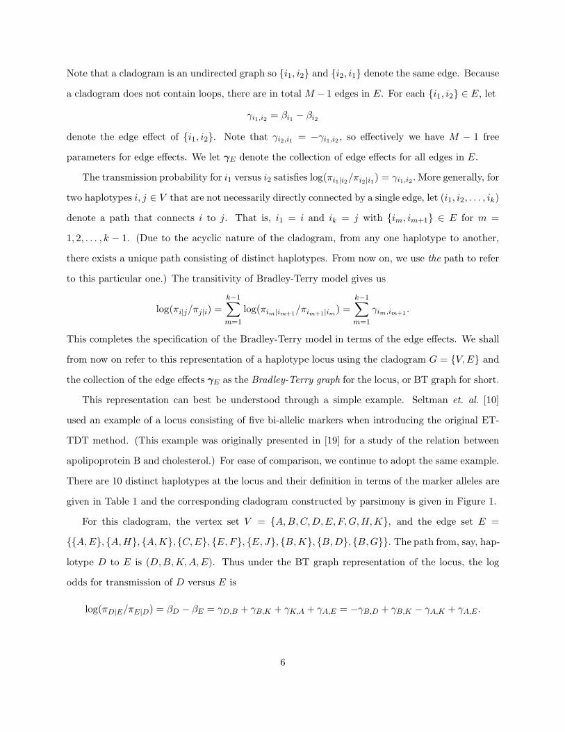
For this cladogram, the vertex set V = {A,B,C,D,E,F,G,H,K}, and the edge set E =
{{A,E}, {A,H}, {A,K}, {C,E}, {E, F}, {E, J}, {B,K}, {B,D}, {B,G}}. The path from, say, hap-
lotype D to E is (D,B,K,A,E). Thus under the BT graph representation of the locus, the log
odds for transmission of D versus E is
log(!D|E/!E|D) = "D " "E = #D,B + #B,K + #K,A + #A,E = "#B,D + #B,K " #A,K + #A,E.
6
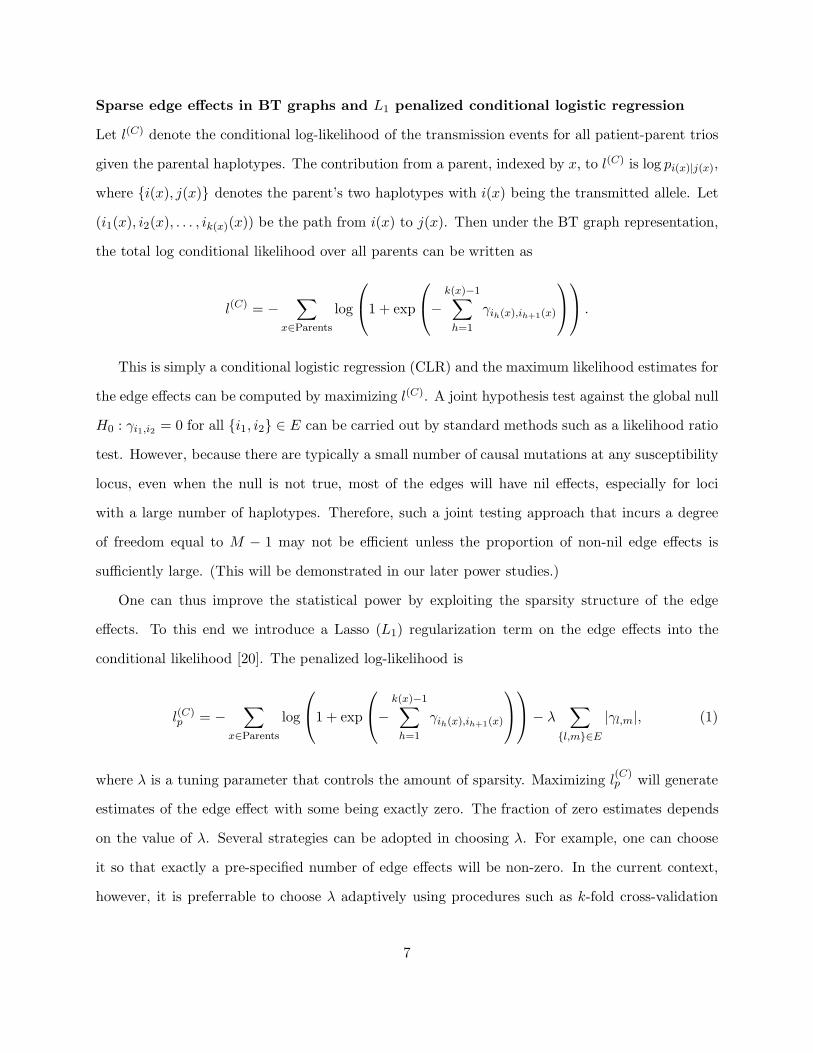
Sparse edge e!ects in BT graphs and L1 penalized conditional logistic regression
Let l(C) denote the conditional log-likelihood of the transmission events for all patient-parent trios
given the parental haplotypes. The contribution from a parent, indexed by x, to l(C) is log pi(x)|j(x),
where {i(x), j(x)} denotes the parent’s two haplotypes with i(x) being the transmitted allele. Let
(i1(x), i2(x), . . . , ik(x)(x)) be the path from i(x) to j(x). Then under the BT graph representation,
the total log conditional likelihood over all parents can be written as
l(C) = "!
x"Parents
log
"
#1 + exp
"
#"
k(x)!1!
h=1
#ih(x),ih+1(x)
$
%
$
% .
This is simply a conditional logistic regression (CLR) and the maximum likelihood estimates for
the edge e!ects can be computed by maximizing l(C). A joint hypothesis test against the global null
H0 : #i1,i2 = 0 for all {i1, i2} # E can be carried out by standard methods such as a likelihood ratio
test. However, because there are typically a small number of causal mutations at any susceptibility
locus, even when the null is not true, most of the edges will have nil e!ects, especially for loci
with a large number of haplotypes. Therefore, such a joint testing approach that incurs a degree
of freedom equal to M " 1 may not be e"cient unless the proportion of non-nil edge e!ects is
su"ciently large. (This will be demonstrated in our later power studies.)
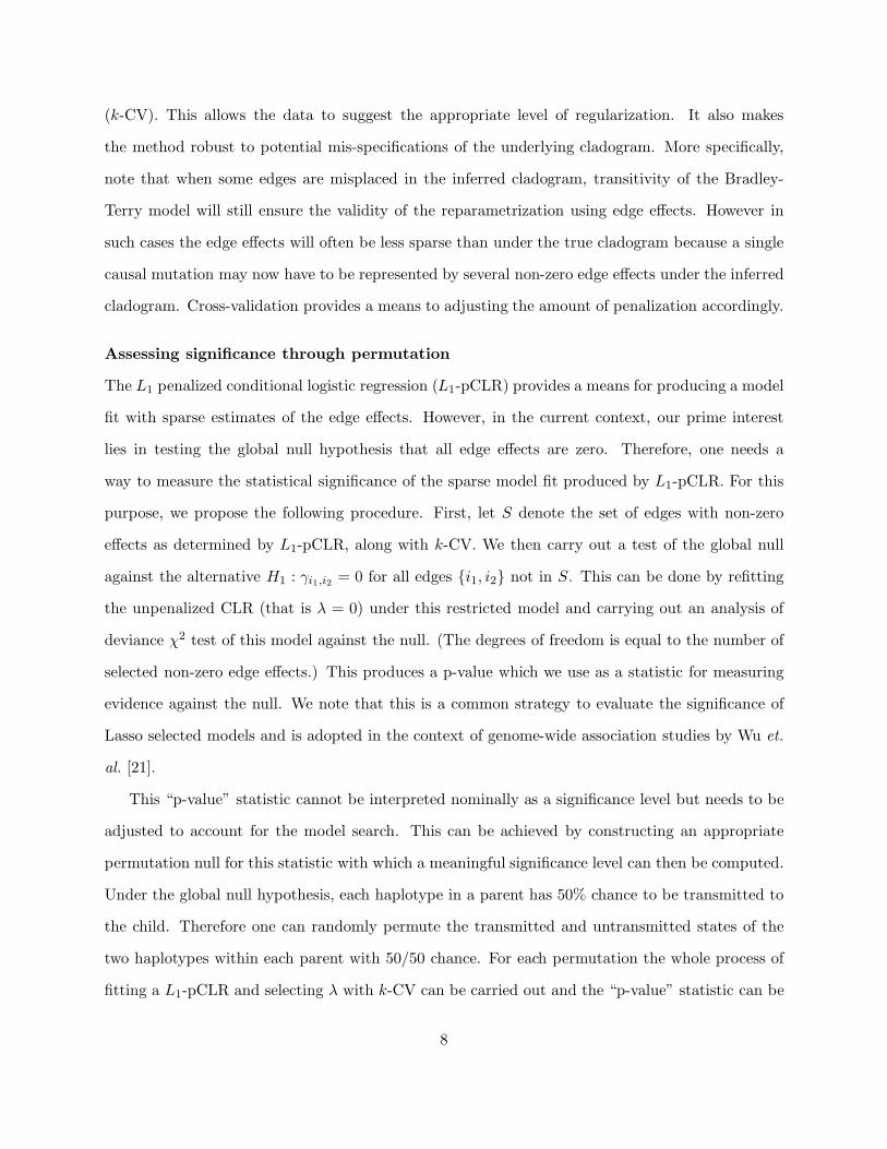
One can thus improve the statistical power by exploiting the sparsity structure of the edge
e!ects. To this end we introduce a Lasso (L1) regularization term on the edge e!ects into the
conditional likelihood [20]. The penalized log-likelihood is
l(C)p = "
!
x"Parents
log
"
#1 + exp
"
#"
k(x)!1!
h=1
#ih(x),ih+1(x)
$
%
$
% " $!
{l,m}"E
|#l,m|, (1)
where $ is a tuning parameter that controls the amount of sparsity. Maximizing l(C)p will generate
estimates of the edge e!ect with some being exactly zero. The fraction of zero estimates depends
on the value of $. Several strategies can be adopted in choosing $. For example, one can choose
it so that exactly a pre-specified number of edge e!ects will be non-zero. In the current context,
however, it is preferrable to choose $ adaptively using procedures such as k-fold cross-validation
7
(k-CV). This allows the data to suggest the appropriate level of regularization. It also makes
the method robust to potential mis-specifications of the underlying cladogram. More specifically,
note that when some edges are misplaced in the inferred cladogram, transitivity of the Bradley-
Terry model will still ensure the validity of the reparametrization using edge e!ects. However in
such cases the edge e!ects will often be less sparse than under the true cladogram because a single
causal mutation may now have to be represented by several non-zero edge e!ects under the inferred
cladogram. Cross-validation provides a means to adjusting the amount of penalization accordingly.
Assessing significance through permutation
The L1 penalized conditional logistic regression (L1-pCLR) provides a means for producing a model
fit with sparse estimates of the edge e!ects. However, in the current context, our prime interest
lies in testing the global null hypothesis that all edge e!ects are zero. Therefore, one needs a
way to measure the statistical significance of the sparse model fit produced by L1-pCLR. For this
purpose, we propose the following procedure. First, let S denote the set of edges with non-zero
e!ects as determined by L1-pCLR, along with k-CV. We then carry out a test of the global null
against the alternative H1 : #i1,i2 = 0 for all edges {i1, i2} not in S. This can be done by refitting
the unpenalized CLR (that is $ = 0) under this restricted model and carrying out an analysis of
deviance %2 test of this model against the null. (The degrees of freedom is equal to the number of
selected non-zero edge e!ects.) This produces a p-value which we use as a statistic for measuring
evidence against the null. We note that this is a common strategy to evaluate the significance of
Lasso selected models and is adopted in the context of genome-wide association studies by Wu et.
al. [21].
This “p-value” statistic cannot be interpreted nominally as a significance level but needs to be
adjusted to account for the model search. This can be achieved by constructing an appropriate
permutation null for this statistic with which a meaningful significance level can then be computed.
Under the global null hypothesis, each haplotype in a parent has 50% chance to be transmitted to
the child. Therefore one can randomly permute the transmitted and untransmitted states of the
two haplotypes within each parent with 50/50 chance. For each permutation the whole process of
fitting a L1-pCLR and selecting $ with k-CV can be carried out and the “p-value” statistic can be
8
computed. After conducting a large number of such permutations, one can then pool the “p-value”
statistics together and get a null distribution. The significance of the originally selected model can
be computed as the proportion of times the permutation “p-value” is smaller, and we can reject
the global null if, say, the significance level is less than 5%.
From now on, we shall refer to the whole procedure of using L1-pCLR with k-CV for model
selection, and using permutation for evaluating the significance level as L1-pCLR based sparse
TDT, or sparse TDT for short. This method is summarized in Box 1.
Box 1 Sparse TDT using L1 penalized conditional logistic regression and k-fold CV
1. Construct the Bradley-Terry graph representation for the locus.
- Construct the cladogram for the locus under investigation using software such as PAUP [22].
- Compute the path between any pair of haplotypes in the cladogram.
3. Fit an L1 penalized (Lasso) conditional logistic regression model in terms of the edge e!ects.
- Use k-fold cross-validation to set the tuning parameter $.
- Given the chosen $, we get a model with a set of non-zero edge e!ects S.
4. Refit the unpenalized conditional logistic regression model using only the edge e!ects in S.
- Carry out an analysis of deviance test of this model against the global null model.
- This produces a p-value statistic, denoted by p.
5. For k = 1, 2, . . . ,N , (e.g. N = 500 is the number of permutations)
- Randomly flip the transmission status of the two haplotypes in each parent.
- For each permuted data set that so arises, repeat Steps 3 and 4 and get a p-value statistic, p(k).
6. Compute the significance level as the proportion of p(k)’s less than p.
- Reject the global null hypothesis of no significant edge e!ects if the significance is < & for
& = 0.05 for example.
Results
In this section we carry out a power study of the proposed method through simulations and compare
it to the original ET-TDT [10] to show the e!ect of incorporating sparsity on the edge e!ects. We
again use the five-maker scenario adopted in [10] as given in Table 1 and Figure 1. We simulate
9

the 10 haplotypes for a population of 100,000 pairs of parents for this five-marker locus according
to the haplotype frequencies given in Table 1. Given these parental haplotypes, we simulate the
haplotypes for one child per parent-pair with equal transmission probability for the two haplotypes
in each parent.
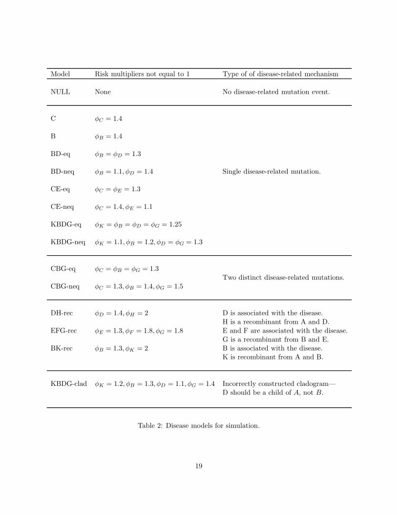
After generating the haplotypes, we simulate the disease status for the children according to
15 di!erent disease models similar to the ones used in [10]. (For ease of comparison, we adopt the
same names for these models as in that paper.) These models were designed to imitate di!erent
mutational and recombinant scenarios that occurred during the evolutionary history of the locus,
according to the underlying cladogram for the alleles (Figure 1). The models are presented in
Table 2. In all of these models, the baseline disease risk for the children population is p0 = 0.2. For
a child with haplotypes i and j at the locus, where i, j # {A,B,C,D,E,F,G,H, J,K}, the risk of
disease pi,j takes a multiplicative form: pi,j = p0'i'j . Hereafter we refer to 'i as the risk multiplier
of haplotype i. The corresponding risk multipliers of the haplotypes for each of the 15 models are
listed in the middle column of Table 2. Haplotypes that do not contribute to the disease risk, that
is whose risk multiplier is 1, are omitted in the table. Note that although the models presented here
are all multiplicative, our proposed method, being based completely on the conditional likelihood,
does not depend on this particular aspect of the simulation.
For each of the models under consideration, after generating the disease status for the children
population, we sample case-parent trios under three sample sizes—n=500, 750, and 1000—and to
each simulated data set we apply Method I: sparse TDT based on L1-pCLR with 10-fold CV for
model selection and Method II: the original ET-TDT, which uses a Bonferroni-adjusted sequential
testing procedure. For comparison, we apply two additional testing strategies—Method III: CLR
with “strong sparsity”, which fits a sparse model with only one non-zero edge e!ect and Method
IV: CLR with no sparsity imposed, i.e. $ = 0. For Method III, the “strong sparsity” test is carried
out by fitting each of the M " 1 models with a single non-zero edge e!ect and choose the most
significant one as determined by the likelihood ratio test p-value against the null, and correct the
significance level computed through the same permutation procedure as that for L1-pCLR based
sparse TDT. For Method IV we carry out a joint likelihood ratio test against the global null that
10
all edges e!ects are nil with no constraints under the alternative.
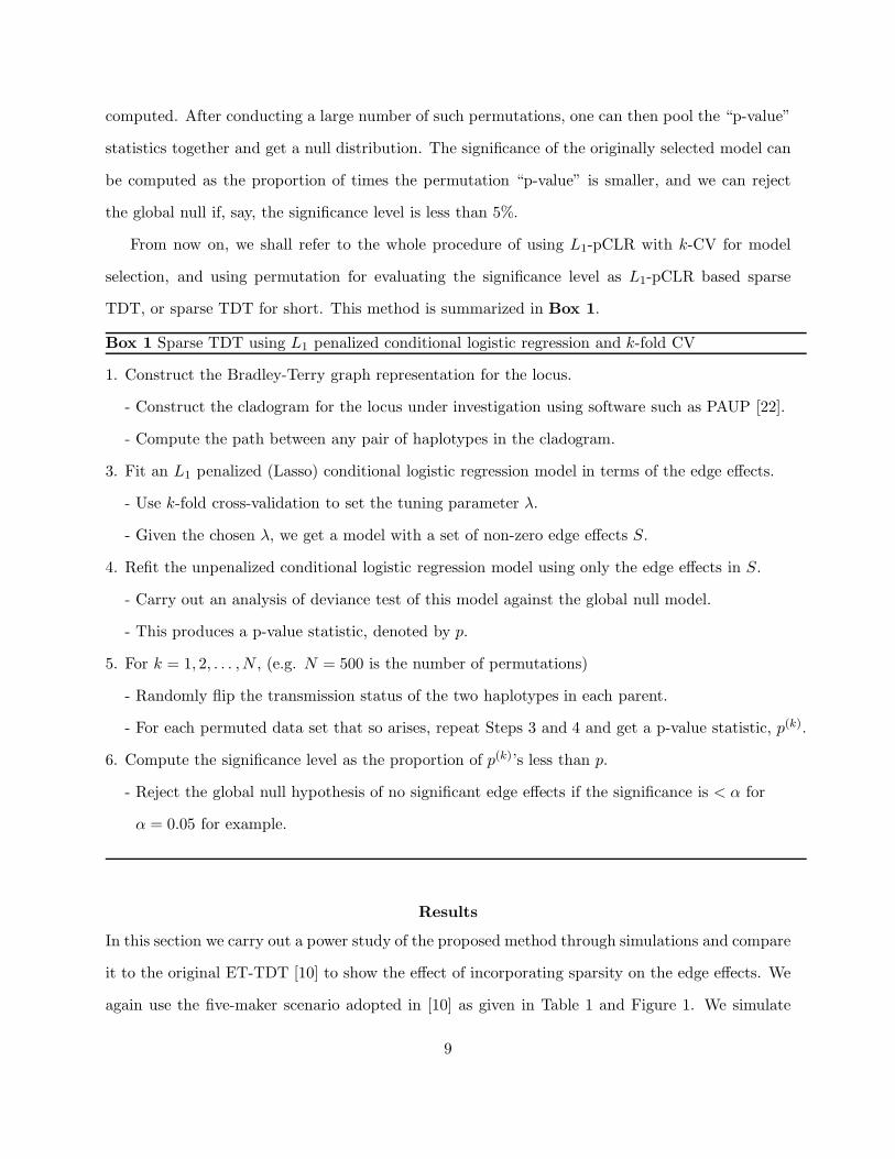
The simulation is repeated 500 times for each model/sample size combination. Each time, 500
permutations are used to evaluate the significance levels. We note that since Method IV is based
on a single global hypothesis test for the entire locus, its p-value can be used without permutation
correction if a single locus is under consideration. (We will discuss strategies for genome-wide
studies in Discussions.) The power is estimated by the fraction of times the null is rejected at
the 5% level. The power at the 5% level (vs sample size) of the four methods are presented in
Figure 2. Note that the power plot for the null model shows that in the current example both
our permutation procedure and the ET-TDT are able to control the Type I error rate at around
5%. Overall, taking sparsity into account pays o! in the power—the L1-pCLR based sparse TDT
consistently outperforms the ET-TDT. In fact it performs the best for all simulated models except
EFG-rec. The good performance of the joint testing approach (labeled as “no sparsity joint” in
Figure 2) is expectable—for that model there are five non-zero edge e!ects out of a total of nine
edges. The performance of the joint testing approach and that of the “strong sparsity” approach,
however, are highly variable and sensitive to the particular underlying disease model. This is not
surprising as neither of these approaches is adaptive to the actual sparsity in the underlying model.
Performance under a larger cladogram
Our proposed approach is based on the idea that the non-zero edge e!ects are sparse. As a result,
one may expect that the gain in performance will increase as the underlying sparsity increases.
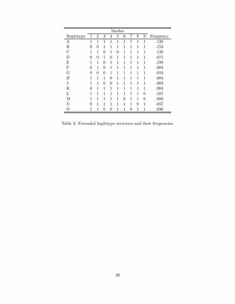
To investigate this, we extend the original cladogram to include four more haplotypes—L, M, N,
O—by adding four more markers into the locus. The corresponding haplotype structures in terms
of the marker alleles are given in Table 3. The extended cladogram is given in Figure 3.
The same simulation procedure under the 15 disease models is repeated for this extended set of
haplotypes, except that now we consider larger sample sizes—n = 500, 1000 and 1500. The power
vs. sample size for the four methods is presented in Figure 4. Several interesting observations can be
made. First, the “no sparsity” joint testing approach performs better than the original ET-TDT
under every model under this extended cladogram. This suggests that the stringent Bonferroni
approach to correct for multiple testing adopted by the ET-TDT may be overly conservative when
11

the number of haplotypes is large. Second, the overall performance of the “strong sparsity” ap-
proach, in comparison to the other methods, is better in this more sparse cladogram, as one would
expect. Finally, L1-pCLR based sparse TDT is again the best performing method overall—the gain
in power over the original ET-TDT is substantial when the underlying model indeed is very sparse.
At the same time, for less sparse models such as EFG-rec and BK-rec (each of them have 5 non-zero
edge e!ects under the extended cladogram), jointly testing all the e!ects actually performed better.
While this phenomenon is something one would expect, it demonstrates itself more clearly in the
extended cladogram than in the original not because of the increased size of the cladogram—in fact
one would expect the joint testing approach to be even more powerful in smaller cladograms where
non-zero edge e!ects constitute a larger proportion of all edge e!ects. Instead, this is probably
due to a combination of two reasons: (1) the frequencies of the disease-related haplotypes have
decreased in the simulation for the extended cladogram, and (2) under the extended cladogram,
the BD-rec model has one extra non-zero edge e!ect.
Discussion
In this work we have proposed an extension to the evolutionary-tree TDT for testing haplotype
transmission disequilibrium in case-parent trios. Like the original ET-TDT, our proposed method
utilizes evolutionary information of the locus through the corresponding cladogram. The original
ET-TDT uses the cladogram as a guide for constructing hypotheses thereby reducing the number of
tests, while we, in addition, use the cladogram as a way to exploit sparsity in mutational events. In
particular, we have introduced the notion of a Bradley-Terry graph by modeling the transmission
event of each parent conditional on his/her haplotypes with a Bradley-Terry model parameterized
in terms of the edges in the underlying cladogram. This allows us to impose sparsity over these edge
e!ects by simply introducing an L1 penalty term into the conditional likelihood. The motivation
for imposing sparsity on the edge e!ects is that the causal mutations for diseases are rare and so
each susceptibility locus is expected to contain at most a small number of them.
One may consider imposing sparsity directly on the haplotype e!ects instead of the edge e!ects.
For example, one can impose sparsity on the di!erence between the e!ect of the most common
haplotype and that of the other ones. In doing so, one eliminates the need for constructing the
12
cladogram, but at the same time does not utilize any evolutionary information. This is undesirable
because even a single mutational event in the evolutionary history could lead to a large number
of haplotypes with “non-zero” e!ects. (For example, consider the model KBDG-eq in our power
study.) In our framework, evolutionary information is utilized through the assumption that a small
number of causal mutations may be embedded in a small number of edge e!ects.
While we have developed our method in the context of testing a single locus, the framework
can be applied in genome-wide or candidate gene studies, where there are often a large number of
genetic loci to test for potential linkage and association. One conceptually easy way to carry out
the test over multiple loci is to use the significance level of each locus computed through locus-by-
locus permutation. For example, one can simply apply to these locus-specific permutation p-values
a standard multiple testing adjustment such as a Bonferroni correction. However, in situations
where the number of loci is large, the adjusted significance threshold of nominal p-values can be
very small, e.g. < 10!5, and therefore it can require a prohibitively large number of permutations
to estimate p-values up to this level of precision for all the loci. In this case, a useful strategy is
to proceed in multiple stages. For example, one can start by running 1,000 permutation for each
locus and then find those that are significant at the 1% level, and run 100,000 permutations for
each of these and find those that are significant at 0.01%, and so on and so forth.
An alternative strategy is to construct an appropriate permutation null distribution for the
nominal significance level of the most significant sparse model over all candidate loci, denoted by
pL1
min. In designing the appropriate permutation procedure, if one’s goal is to imitate as closely
as possible the underlying biological process, one should ideally maintain the linkage structure
across the loci—the more linked two loci are with each other, the more likely they should be
permuted together. A randomization procedure like this will break down the linkage and the linkage
disequilibrium between the loci and the disease status as is desired in building the null. The exact
manner in which such randomization should be carried out is interesting but beyond the scope of
this paper. In the current context, however, there is a simple “proxy” to this procedure. That is
to permute the transmission states at all loci for each parent together. In other words, for each
parent we flip a coin, and if the coin shows head, we swap the transmitted and the untransmitted
13
haplotypes at all loci for that parent. If it shows tail, we leave the transmission states of the
haplotypes unchanged at all loci for that parent. For each such permutation we recompute pL1
min.
The permutation null distribution we get by pooling these values can then be used for calculating
genome-wide p-values. This simplified permutation procedure does not imitate the actual linkage
among the markers, but it does break down both the linkage and the linkage disequilibrium between
the loci and the disease status, while maintaining the linkage disequilibrium among the markers.
Our method is designed based on the assumption that there is no ambiguity in determining
what haplotype is transmitted to the child from each parent. As the density of genetic markers gets
higher, the problem of ambiguous haplotype phase will occur less and less frequently. Nevertheless,
simple strategies to deal with ambiguous haplotype phase include imputing the phase with the
most likely allele [13]. As mentioned at the beginning of this work, experimental technologies are
now available that allow us to attain phased genotype information from the subjects directly [1],
eliminating the phase problem completely. While the development of such technology is still in its
early stage and so the cost is relatively high at the time of this writing, we expect their use in the
future to become more prevalent.
Acknowledgment
WHW is supported in part by NIH grants R01HG004634 and R01HG005717, and NSF grant
DMS-0906044. ABO is supported by NSF-DMS0906056. Much of the computation in this work
was carried out on computer resources supported by NSF awards CNS-0619926 and DMS-0821823.
References
[1] Yang, H., Chen, X., and Wong, W. H. (2011). Completely phased genome sequencing through
chromosome sorting. P. Natl. Acad. Sci. USA. 108, 12–17.
[2] Falk, C. T. and Rubinstein, P. (1987). Haplotype relative risks: an easy reliable way to
construct a proper control sample for risk calculations. Ann. Hum. Genet. 51, 227–233.
[3] Ott, J. (1989). Statistical properties of the haplotype relative risk. Genet. Epidemiol. 6.
14
[4] Spielman, R. S., McGinnis, R. E., and Ewens, W. J. (1993). Transmission test for linkage
disequilibrium: the insulin gene region and insulin-dependent diabetes mellitus (iddm). Am.
J. Hum. Genet. 52, 506.
[5] Ewens, W. J. and Spielman, R. S. (1995). The transmission/disequilibrium test: history,
subdivision, and admixture. Am. J. Hum. Genet. 57, 455.
[6] Spielman, R. S. and Ewens, W. J. (1996). The TDT and other family-based tests for linkage
disequilibrium and association. Am. J. Hum. Genet. 59, 983.
[7] Lazzeroni, L. and Lange, K. (1998). A conditional inference framework for extending the
transmission/disequilibrium test. Hum. Hered. 48, 67–81.
[8] Clayton, D. (1999). A generalization of the transmission/disequilibrium test for uncertain-
haplotype transmission. Am. J. Hum. Genet. 4, 1170–1177.
[9] Clayton, D. and Jones, H. (1999). Transmission/disequilibrium tests for extended marker
haplotypes. Am. J. Hum. Genet. 65, 1161–1169.
[10] Seltman, H., Roeder, K., and Devlin, B. (2001). Transmission/disequilibrium test meets mea-
sured haplotype analysis: family-based association analysis guided by evolution of haplotypes.
Am. J. Hum. Genet. 68, 1250–1263.
[11] Rabinowitz, D. and Laird, N. (2000). A unified approach to adjusting association tests for pop-
ulation admixture with arbitrary pedigree structure and arbitrary missing marker information.
Hum. Hered. 50, 211–223.
[12] Zhao, H., Zhang, S., Merikangas, K. R., Trixler, M., Wildenauer, D. B., Sun, F., and Kidd,
K. K. (2000). Transmission/disequilibrium tests using multiple tightly linked markers. Am.
J. Hum. Genet. 67, 936.
[13] Zhang, S., Sha, Q., Chen, H.-S., Dong, J., and Jiang, R. (2003). Transmission/disequilibrium
test based on haplotype sharing for tightly linked markers. Am. J. Hum. Genet. 73, 566–579.
15
[14] Templeton, A. R., Boerwinkle, E., and Sing, C. F. (1987). A cladistic analysis of phenotypic
associations with haplotypes inferred from restriction endonuclease mapping. i. basic theory
and an analysis of alcohol dehydrogenase activity in drosophila. Genetics 117, 343.
[15] Templeton, A. R., Sing, C. F., Kessling, A., and Humphries, S. (1988). A cladistic analysis
of phenotype associations with haplotypes inferred from restriction endonuclease mapping. ii.
the analysis of natural populations. Genetics 120, 1145.
[16] Templeton, A. R., Crandall, K. A., and Sing, C. F. (1992). A cladistic analysis of phenotypic
associations with haplotypes inferred from restriction endonuclease mapping and dna sequence
data. iii. cladogram estimation. Genetics 132, 619.
[17] Templeton, A. and Sing, C. F. (1993). A cladistic analysis of phenotypic associations with
haplotypes inferred from restriction endonuclease mapping. iv. nested analyses with cladogram
uncertainty and recombination. Genetics 134, 659.
[18] Templeton, A. R. (1995). A cladistic analysis of phenotypic associations with haplotypes
inferred from restriction endonuclease mapping or dna sequencing. v. analysis of case/control
sampling designs: Alzheimer’s disease and the apoprotein e locus. Genetics 140, 403.
[19] Hallman, D. M., Visvikis, S., Steinmetz, J., and Boerwinkle, E. (1994). The e!ect of variation
in the apolipoprotein B gene on plasma lipid and apolipoprotein B levels i. a likelihood-based
approach to cladistic analysis. Ann. Hum. Genet. 58, 35–64.
[20] Tibshirani, R. (1996). Regression Shrinkage and Selection Via the Lasso. Journal of the Royal
Statistical Society, Series B 58, 267–288.
[21] Wu, T. T., Chen, Y. F., Hastie, T., Sobel, E., and Lange, K. (2009). Genome-wide association
analysis by lasso penalized logistic regression. Bioinformatics 25, 714–721.
[22] Swo!ord, D. L. (2003). PAUP* Phylogenetic Analysis Using Parsimony (*and Other Methods)
Version 4.04beta. (Sinauer Associates, Sunderland, Massachusetts).
16
Table captions
Table 1: Haplotype structures and relative frequencies. This example is from [19] and was adopted
in [10]. The frequencies sum up to 1.001 and we normalize them in the computation.
Table 2: Disease models for simulation.
Table 3: Extended haplotype structure and their frequencies.
17

Tables
Marker
Haplotype 1 2 3 4 5 FrequencyA 1 1 1 1 1 .180B 0 0 1 1 1 .214C 1 1 0 1 0 .194D 0 0 1 0 1 .100E 1 1 0 1 1 .277F 0 1 0 1 1 .006G 0 0 0 1 1 .014H 1 1 1 0 1 .006J 1 1 0 0 1 .004K 0 1 1 1 1 .006
Table 1: Haplotype structures and relative frequencies. This example is from [19] and was adopted
in [10]. The frequencies sum up to 1.001 and we normalize them in the computation.
18
Model Risk multipliers not equal to 1 Type of of disease-related mechanism
NULL None No disease-related mutation event.
C 'C = 1.4
B 'B = 1.4
BD-eq 'B = 'D = 1.3
BD-neq 'B = 1.1,'D = 1.4 Single disease-related mutation.
CE-eq 'C = 'E = 1.3
CE-neq 'C = 1.4,'E = 1.1
KBDG-eq 'K = 'B = 'D = 'G = 1.25
KBDG-neq 'K = 1.1,'B = 1.2,'D = 'G = 1.3
CBG-eq 'C = 'B = 'G = 1.3Two distinct disease-related mutations.
CBG-neq 'C = 1.3,'B = 1.4,'G = 1.5
DH-rec 'D = 1.4,'H = 2 D is associated with the disease.H is a recombinant from A and D.
EFG-rec 'E = 1.3,'F = 1.8,'G = 1.8 E and F are associated with the disease.G is a recombinant from B and E.
BK-rec 'B = 1.3,'K = 2 B is associated with the disease.K is recombinant from A and B.
KBDG-clad 'K = 1.2,'B = 1.3,'D = 1.1,'G = 1.4 Incorrectly constructed cladogram—D should be a child of A, not B.
Table 2: Disease models for simulation.
19
MarkerHaplotype 1 2 3 4 5 6 7 8 9 FrequencyA 1 1 1 1 1 1 1 1 1 .128B 0 0 1 1 1 1 1 1 1 .153C 1 1 0 1 0 1 1 1 1 .138D 0 0 1 0 1 1 1 1 1 .071E 1 1 0 1 1 1 1 1 1 .198F 0 1 0 1 1 1 1 1 1 .004G 0 0 0 1 1 1 1 1 1 .010H 1 1 1 0 1 1 1 1 1 .004J 1 1 0 0 1 1 1 1 1 .003K 0 1 1 1 1 1 1 1 1 .004L 1 1 1 1 1 1 1 1 0 .107M 1 1 1 1 1 0 1 1 0 .086N 0 1 1 1 1 1 1 0 1 .057O 1 1 0 0 1 1 0 1 1 .036
Table 3: Extended haplotype structure and their frequencies.
20
Figure legends
Figure 1: Cladogram of the haplotypes as presented in Table 1. This example is originally from [19]
and was adopted in [10].
Figure 2: Power at 5% level vs. sample size under the 15 models for four methods: (1) red solid
represents sparse TDT based on L1-pCLR with 10-fold cross-validation; (2) black solid represents
ET-TDT; (3) blue dashed represents CLR with “strong sparsity”; (4) green dashed represents joint
testing using CLR with no sparsity.
Figure 3: Extended cladogram. Four additional haplotypes L, M , N , and O are added.
Figure 4: Power at 5% level vs. sample size for the extended cladogram under the 15 models for four
methods: (1) red solid represents sparse TDT based on L1-pCLR with 10-fold cross-validation; (2)
black solid represents ET-TDT; (3) blue dashed represents CLR with “strong sparsity”; (4) green
dashed represents joint testing using CLR with no sparsity.
21

Illustrations
Figure 1: Cladogram of the haplotypes as presented in Table 1. This example is originally from [19]and was adopted in [10].
22

n
Powe
r
n
Powe
r
NULL
n
Powe
r
500 750 1000
0.0
0.2
0.4
0.6
0.8
1.0
NULL
n
Powe
r
500 750 1000
0.0
0.2
0.4
0.6
0.8
1.0
NULL
n
Powe
r
500 750 1000
0.0
0.2
0.4
0.6
0.8
1.0
nPo
wer
nPo
wer
C
nPo
wer
500 750 1000
0.0
0.2
0.4
0.6
0.8
1.0
C
nPo
wer
500 750 1000
0.0
0.2
0.4
0.6
0.8
1.0
C
nPo
wer
500 750 1000
0.0
0.2
0.4
0.6
0.8
1.0
n
Powe
r
n
Powe
r
B
n
Powe
r
500 750 1000
0.0
0.2
0.4
0.6
0.8
1.0
B
n
Powe
r
500 750 1000
0.0
0.2
0.4
0.6
0.8
1.0
B
n
Powe
r
500 750 1000
0.0
0.2
0.4
0.6
0.8
1.0
n
Powe
r
n
Powe
r
BD−eq
n
Powe
r
500 750 1000
0.0
0.2
0.4
0.6
0.8
1.0
BD−eq
n
Powe
r
500 750 1000
0.0
0.2
0.4
0.6
0.8
1.0
BD−eq
n
Powe
r
500 750 1000
0.0
0.2
0.4
0.6
0.8
1.0
n
Powe
r
n
Powe
r
BD−neq
n
Powe
r
500 750 1000
0.0
0.2
0.4
0.6
0.8
1.0
BD−neq
n
Powe
r
500 750 1000
0.0
0.2
0.4
0.6
0.8
1.0
BD−neq
n
Powe
r
500 750 1000
0.0
0.2
0.4
0.6
0.8
1.0
n
Powe
r
n
Powe
r
CE−eq
n
Powe
r
500 750 1000
0.0
0.2
0.4
0.6
0.8
1.0
CE−eq
n
Powe
r
500 750 1000
0.0
0.2
0.4
0.6
0.8
1.0
CE−eq
n
Powe
r
500 750 1000
0.0
0.2
0.4
0.6
0.8
1.0
n
Powe
r
n
Powe
r
CE−neq
n
Powe
r
500 750 10000.
00.
20.
40.
60.
81.
0
CE−neq
n
Powe
r
500 750 10000.
00.
20.
40.
60.
81.
0
CE−neq
n
Powe
r
500 750 10000.
00.
20.
40.
60.
81.
0
n
Powe
r
n
Powe
r
KBDG−eq
n
Powe
r
500 750 1000
0.0
0.2
0.4
0.6
0.8
1.0
KBDG−eq
n
Powe
r
500 750 1000
0.0
0.2
0.4
0.6
0.8
1.0
KBDG−eq
n
Powe
r
500 750 1000
0.0
0.2
0.4
0.6
0.8
1.0
n
Powe
r
n
Powe
r
KBDG−neq
n
Powe
r
500 750 1000
0.0
0.2
0.4
0.6
0.8
1.0
KBDG−neq
n
Powe
r
500 750 1000
0.0
0.2
0.4
0.6
0.8
1.0
KBDG−neq
n
Powe
r
500 750 1000
0.0
0.2
0.4
0.6
0.8
1.0
n
Powe
r
n
Powe
r
CBG−eq
n
Powe
r
500 750 1000
0.0
0.2
0.4
0.6
0.8
1.0
CBG−eq
n
Powe
r
500 750 1000
0.0
0.2
0.4
0.6
0.8
1.0
CBG−eq
n
Powe
r
500 750 1000
0.0
0.2
0.4
0.6
0.8
1.0
n
Powe
r
n
Powe
r
CBG−neq
n
Powe
r
500 750 1000
0.0
0.2
0.4
0.6
0.8
1.0
CBG−neq
n
Powe
r
500 750 1000
0.0
0.2
0.4
0.6
0.8
1.0
CBG−neq
n
Powe
r
500 750 1000
0.0
0.2
0.4
0.6
0.8
1.0
n
Powe
r
n
Powe
r
DH−rec
n
Powe
r
500 750 1000
0.0
0.2
0.4
0.6
0.8
1.0
DH−rec
n
Powe
r
500 750 1000
0.0
0.2
0.4
0.6
0.8
1.0
DH−rec
n
Powe
r
500 750 1000
0.0
0.2
0.4
0.6
0.8
1.0
n
Powe
r
n
Powe
r
EFG−rec
n
Powe
r
500 750 1000
0.0
0.2
0.4
0.6
0.8
1.0
EFG−rec
n
Powe
r
500 750 1000
0.0
0.2
0.4
0.6
0.8
1.0
EFG−rec
n
Powe
r
500 750 1000
0.0
0.2
0.4
0.6
0.8
1.0
n
Powe
r
n
Powe
r
BK−rec
n
Powe
r
500 750 1000
0.0
0.2
0.4
0.6
0.8
1.0
BK−rec
n
Powe
r
500 750 1000
0.0
0.2
0.4
0.6
0.8
1.0
BK−rec
n
Powe
r
500 750 1000
0.0
0.2
0.4
0.6
0.8
1.0
n
Powe
r
n
Powe
r
KBDG−clad
n
Powe
r
500 750 1000
0.0
0.2
0.4
0.6
0.8
1.0
KBDG−clad
n
Powe
r
500 750 1000
0.0
0.2
0.4
0.6
0.8
1.0
KBDG−clad
n
Powe
r
500 750 1000
0.0
0.2
0.4
0.6
0.8
1.0
L1−pCLR with 10−CVET−TDTStrong sparsityNo sparsity joint
Figure 2: Power at 5% level vs. sample size under the 15 models for four methods: (1) red solidrepresents sparse TDT based on L1-pCLR with 10-fold cross-validation; (2) black solid representsET-TDT; (3) blue dashed represents CLR with “strong sparsity”; (4) green dashed represents jointtesting using CLR with no sparsity.
23
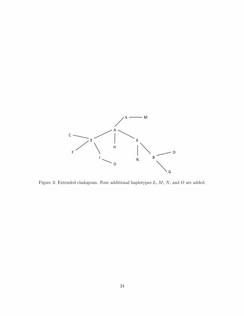
Figure 3: Extended cladogram. Four additional haplotypes L, M , N , and O are added.
24

n
Powe
r
n
Powe
r
NULL
n
Powe
r
500 1000 1500
0.0
0.2
0.4
0.6
0.8
1.0
NULL
n
Powe
r
500 1000 1500
0.0
0.2
0.4
0.6
0.8
1.0
NULL
n
Powe
r
500 1000 1500
0.0
0.2
0.4
0.6
0.8
1.0
nPo
wer
nPo
wer
C
nPo
wer
500 1000 1500
0.0
0.2
0.4
0.6
0.8
1.0
C
nPo
wer
500 1000 1500
0.0
0.2
0.4
0.6
0.8
1.0
C
nPo
wer
500 1000 1500
0.0
0.2
0.4
0.6
0.8
1.0
n
Powe
r
n
Powe
r
B
n
Powe
r
500 1000 1500
0.0
0.2
0.4
0.6
0.8
1.0
B
n
Powe
r
500 1000 1500
0.0
0.2
0.4
0.6
0.8
1.0
B
n
Powe
r
500 1000 1500
0.0
0.2
0.4
0.6
0.8
1.0
n
Powe
r
n
Powe
r
BD−eq
n
Powe
r
500 1000 1500
0.0
0.2
0.4
0.6
0.8
1.0
BD−eq
n
Powe
r
500 1000 1500
0.0
0.2
0.4
0.6
0.8
1.0
BD−eq
n
Powe
r
500 1000 1500
0.0
0.2
0.4
0.6
0.8
1.0
n
Powe
r
n
Powe
r
BD−neq
n
Powe
r
500 1000 1500
0.0
0.2
0.4
0.6
0.8
1.0
BD−neq
n
Powe
r
500 1000 1500
0.0
0.2
0.4
0.6
0.8
1.0
BD−neq
n
Powe
r
500 1000 1500
0.0
0.2
0.4
0.6
0.8
1.0
n
Powe
r
n
Powe
r
CE−eq
n
Powe
r
500 1000 1500
0.0
0.2
0.4
0.6
0.8
1.0
CE−eq
n
Powe
r
500 1000 1500
0.0
0.2
0.4
0.6
0.8
1.0
CE−eq
n
Powe
r
500 1000 1500
0.0
0.2
0.4
0.6
0.8
1.0
n
Powe
r
n
Powe
r
CE−neq
n
Powe
r
500 1000 15000.
00.
20.
40.
60.
81.
0
CE−neq
n
Powe
r
500 1000 15000.
00.
20.
40.
60.
81.
0
CE−neq
n
Powe
r
500 1000 15000.
00.
20.
40.
60.
81.
0
n
Powe
r
n
Powe
r
KBDG−eq
n
Powe
r
500 1000 1500
0.0
0.2
0.4
0.6
0.8
1.0
KBDG−eq
n
Powe
r
500 1000 1500
0.0
0.2
0.4
0.6
0.8
1.0
KBDG−eq
n
Powe
r
500 1000 1500
0.0
0.2
0.4
0.6
0.8
1.0
n
Powe
r
n
Powe
r
KBDG−neq
n
Powe
r
500 1000 1500
0.0
0.2
0.4
0.6
0.8
1.0
KBDG−neq
n
Powe
r
500 1000 1500
0.0
0.2
0.4
0.6
0.8
1.0
KBDG−neq
n
Powe
r
500 1000 1500
0.0
0.2
0.4
0.6
0.8
1.0
n
Powe
r
n
Powe
r
CBG−eq
n
Powe
r
500 1000 1500
0.0
0.2
0.4
0.6
0.8
1.0
CBG−eq
n
Powe
r
500 1000 1500
0.0
0.2
0.4
0.6
0.8
1.0
CBG−eq
n
Powe
r
500 1000 1500
0.0
0.2
0.4
0.6
0.8
1.0
n
Powe
r
n
Powe
r
CBG−neq
n
Powe
r
500 1000 1500
0.0
0.2
0.4
0.6
0.8
1.0
CBG−neq
n
Powe
r
500 1000 1500
0.0
0.2
0.4
0.6
0.8
1.0
CBG−neq
n
Powe
r
500 1000 1500
0.0
0.2
0.4
0.6
0.8
1.0
n
Powe
r
n
Powe
r
DH−rec
n
Powe
r
500 1000 1500
0.0
0.2
0.4
0.6
0.8
1.0
DH−rec
n
Powe
r
500 1000 1500
0.0
0.2
0.4
0.6
0.8
1.0
DH−rec
n
Powe
r
500 1000 1500
0.0
0.2
0.4
0.6
0.8
1.0
n
Powe
r
n
Powe
r
EFG−rec
n
Powe
r
500 1000 1500
0.0
0.2
0.4
0.6
0.8
1.0
EFG−rec
n
Powe
r
500 1000 1500
0.0
0.2
0.4
0.6
0.8
1.0
EFG−rec
n
Powe
r
500 1000 1500
0.0
0.2
0.4
0.6
0.8
1.0
n
Powe
r
n
Powe
r
BK−rec
n
Powe
r
500 1000 1500
0.0
0.2
0.4
0.6
0.8
1.0
BK−rec
n
Powe
r
500 1000 1500
0.0
0.2
0.4
0.6
0.8
1.0
BK−rec
n
Powe
r
500 1000 1500
0.0
0.2
0.4
0.6
0.8
1.0
n
Powe
r
n
Powe
r
KBDG−clad
n
Powe
r
500 1000 1500
0.0
0.2
0.4
0.6
0.8
1.0
KBDG−clad
n
Powe
r
500 1000 1500
0.0
0.2
0.4
0.6
0.8
1.0
KBDG−clad
n
Powe
r
500 1000 1500
0.0
0.2
0.4
0.6
0.8
1.0
L1−pCLR with 10−CVET−TDTStrong sparsityNo sparsity joint
Figure 4: Power at 5% level vs. sample size for the extended cladogram under the 15 models for fourmethods: (1) red solid represents sparse TDT based on L1-pCLR with 10-fold cross-validation; (2)black solid represents ET-TDT; (3) blue dashed represents CLR with “strong sparsity”; (4) greendashed represents joint testing using CLR with no sparsity.
25