A Sparse Texture Representation Using

Local Affine Regions

Svetlana Lazebnik1 Cordelia Schmid2 Jean Ponce1

slazebni@uiuc.edu cordelia.schmid@inrialpes.fr ponce@cs.uiuc.edu

1 Beckman Institute 2 INRIA Rhone-Alpes,University of Illinois 665 Avenue de l’Europe,405 N. Mathews Ave. 38330 Montbonnot, France

Urbana, IL 61801, USA

Abstract

This article introduces a texture representation suitable for recognizing images of textured

surfaces under a wide range of transformations, including viewpoint changes and non-rigid

deformations. At the feature extraction stage, a sparse set of affine Harris and Laplacian

regions is found in the image. Each of these regions can be thought of as a texture element

having a characteristic elliptic shape and a distinctive appearance pattern. This pattern is

captured in an affine-invariant fashion via a process of shape normalization followed by the

computation of two novel descriptors, the spin image and the RIFT descriptor. When affine

invariance is not required, the original elliptical shape serves as an additional discriminative

feature for texture recognition. The proposed approach is evaluated in retrieval and classi-

fication tasks using the entire Brodatz database and a publicly available collection of 1000

photographs of textured surfaces taken from different viewpoints.

Keywords: Image Processing and Computer Vision, Feature Measurement, Texture,

Pattern Recognition.

1 Introduction

The automated analysis of image textures has been the topic of extensive research in the past

forty years, dating back at least to Julesz in 1962 [14]. Existing techniques for modeling tex-

ture include co-occurrence statistics [11, 14], filter banks [29, 37], and random fields [30, 51].

Unfortunately, most of these methods make restrictive assumptions about the nature of the

input texture (e.g., stationarity), and they are not, in general, invariant with respect to

2D similarity and affine transformations, much less to 3D transformations such as view-

point changes and non-rigid deformations of the textured surface. This lack of geometric

invariance presents a serious limitation for many applications of texture analysis, includ-

ing wide-baseline stereo matching [1, 40, 41, 45], indexing and retrieval in image and video

databases [32, 42, 43, 44], and classification of images of materials [46, 47].

In this article, we set out to develop a texture representation that is invariant to geometric

transformations that can be locally approximated by an affine model. Since sufficiently

small patches on the surfaces of smooth 3D objects are always approximately planar, local

affine invariants are appropriate for modeling not only global 2D affine transformations of

the image, but also perspective distortions that arise in imaging a planar textured surface,

as well as non-rigid deformations that preserve the locally flat structure of the surface,

such as the bending of paper or cloth. Specifically, our proposed texture representation

works by characterizing the appearance of distinguished local affine regions in the image.

Like other approaches based on textons, or primitive texture elements [7, 22, 46, 47], our

method involves representing distributions of 2D image features; unlike these, however, it

performs shape selection, ensuring that descriptors are computed over neighborhoods whose

shape is adapted to changes in surface orientation and scale caused by camera movements

or scene deformations. In addition, our method performs spatial selection by computing

descriptors at a sparse set of image locations output by local affine region detectors. This

is a significant departure from the traditional feature extraction framework, which involves

2

(a) (b) (c) (d)

Figure 1: The effect of spatial selection on a texton dictionary. (a) Original texture image.(b) Top 20 textons found by clustering all 13 × 13 patches of the image. (c) A sparse set ofregions found by the Laplacian detector described in Section 3.1. Each region is normalizedto yield a 13 × 13 patch. (d) Textons obtained by clustering the normalized patches.1

processing every pixel location in the image. Apart from being memory- and computation-

intensive, this dense approach produces redundant texton dictionaries that may include,

for instance, many slightly shifted versions of the same basic element [28]. As Figure 1

illustrates, spatial selection is an effective way to reduce this redundancy.

Our approach consists of the following steps (see also Figure 2):

1. Extract a sparse set of affine regions2 in the shape of ellipses from a texture image.

The two region detectors used for this purpose are described in Section 3.1.

2. Normalize the shape of each elliptical region by transforming it into a circle. This

reduces the affine ambiguity to a rotational one. Full affine invariance is achieved by

computing rotation-invariant descriptors over the normalized regions. In Section 3.2,

we introduce two novel rotation-invariant descriptors: one based on spin images used

for matching range data [13], and one based on Lowe’s SIFT descriptor [27].

3. Perform clustering on the affine-invariant descriptors to obtain a more compact repre-

1For the sake of this illustration, we disregard the orthogonal ambiguity inherent in the normalizationprocess (see Section 3.1 for details). Because we are clustering the normalized patches themselves, insteadof rotation-invariant descriptors as in Section 3.2, the resulting description of patch appearance in this caseis rotation-dependent. This can be seen from the fact that the second and third clusters of (d) are rotatedversions of each other.

2This is an abbreviation of the more accurate term affine-covariant regions, which refers to their theo-retically expected behavior: Namely, the regions found in a picture deformed by some affine transformationshould be the images under the same transformation of the regions found in the original picture.

3

sentation of the distribution of features in each image (Section 3.3). Summarize this

distribution in the form of a signature, containing a representative descriptor from each

cluster and a weight indicating the relative size of the cluster.

4. Compare signatures of different images using the Earth Mover’s Distance (EMD) [38,

39], which is a convenient and effective dissimilarity measure applicable to many types

of image information. The output of this stage is an EMD matrix whose entries record

the distances between each pair of signatures in the database. The EMD matrix can

be used for retrieval and classification tasks, as described in Section 4.1.

� � �

1. Extract affineregions

2. Compute affine-invariant descriptors

3. Find clustersand signatures

4. Compute distancesbetween signatures

Image 1

Image n

�1

�n

d (�i , )�j

Figure 2: The architecture of the feature extraction system proposed in this article.

In Section 4, we will use two datasets to evaluate the capabilities of the proposed tex-

ture representation. The first dataset, introduced in Section 4.2, consists of photographs

of textured surfaces taken from different viewpoints and featuring large scale changes, per-

spective distortions, and non-rigid transformations. It must be noted that, even though our

method relies on implicit assumptions of local flatness and Lambertian appearance, and is

thus theoretically applicable primarily to “albedo textures” due to spatial albedo variations

on smooth surfaces, the results in Section 4.2 show that in practice it also tends to perform

well on “3D textures” arising from local relief variations on a surface. Our second set of

experiments, described in Section 4.3, is carried out on the Brodatz database [4], a collection

of images that features significant inter-class variability, but no geometric transformations

4

between members of the same class. Because affine invariance is not required in this case, we

modify the basic feature extraction framework to use neighborhood shape as a discriminative

feature to improve performance.

2 Previous Work

Before presenting the details of our approach (Section 3), let us briefly discuss a number

of texture models aimed at achieving invariance under various geometric transformations.

Early research in this domain has concentrated on global 2D image transformations, such as

rotation and scaling [5, 30]. However, such models do not accurately capture the effects of 3D

transformations (even in-plane rotations) of textured surfaces. More recently, there has been

a great deal of interest in recognizing images of textured surfaces subjected to lighting and

viewpoint changes [7, 8, 22, 26, 46, 47, 49]. A few methods [22, 26, 49] are based on explicit

reasoning about the 3D structure of the surface, which may involve registering samples of

a material so that the same pixel across different images corresponds to the same physical

point on the surface [22] or applying photometric stereo to reconstruct the depth map of the

3D texture [26, 49]. While such approaches capture the appearance variations of 3D surfaces

in a principled manner, they require specially calibrated datasets collected under controlled

laboratory conditions. For example, the 3D texton representation of Leung and Malik [22]

naturally lends itself to the task of classifying a “stack” of registered images of a test material

with known imaging parameters, but its applicability is limited in most practical situations.

In this presentation, we are interested in classifying unregistered texture images. This

problem has been addressed by Cula and Dana [7] and Varma and Zisserman [46, 47], who

have developed several dense 2D texton-based representations capable of very high accuracy

on the challenging Columbia-Utrecht reflectance and texture (CUReT) database [8]. The

descriptors used in these representations are filter bank outputs [7, 46] and raw pixel val-

ues [47]. Even though these methods have been successful in the complex task of classifying

images of materials despite significant appearance changes, the representations themselves

5

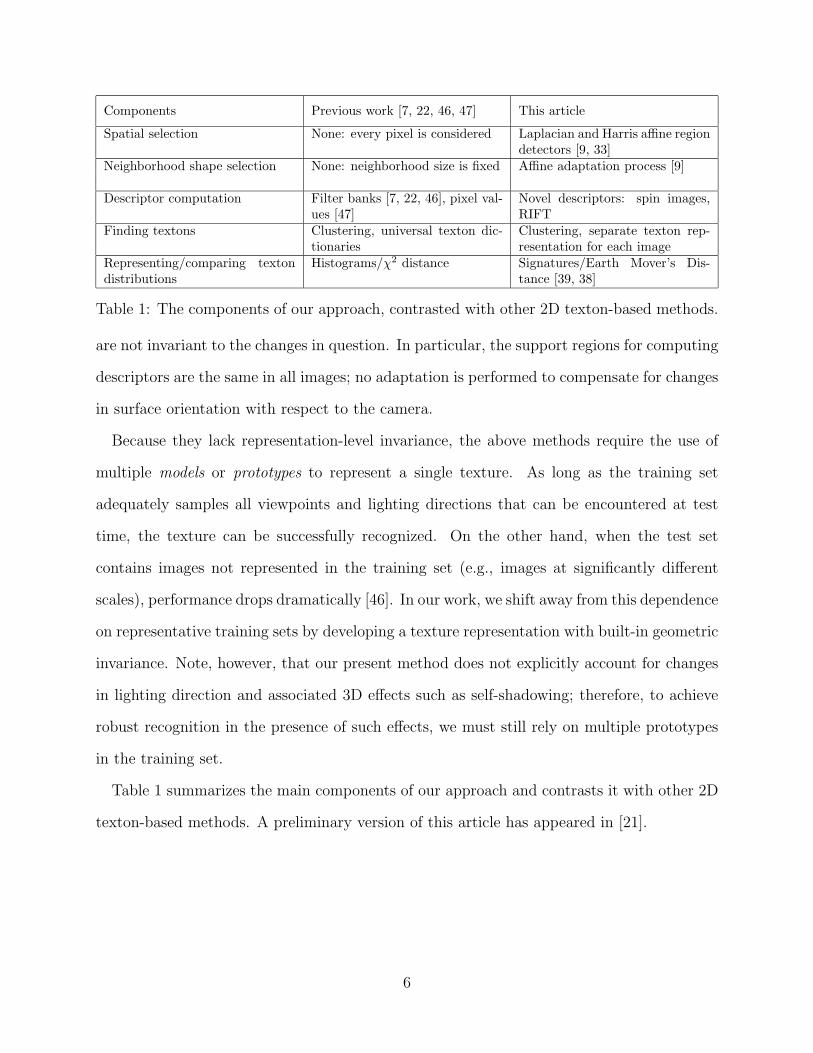
Components Previous work [7, 22, 46, 47] This article

Spatial selection None: every pixel is considered Laplacian and Harris affine regiondetectors [9, 33]

Neighborhood shape selection None: neighborhood size is fixed Affine adaptation process [9]

Descriptor computation Filter banks [7, 22, 46], pixel val-ues [47]

Novel descriptors: spin images,RIFT

Finding textons Clustering, universal texton dic-tionaries

Clustering, separate texton rep-resentation for each image

Representing/comparing textondistributions

Histograms/χ2 distance Signatures/Earth Mover’s Dis-tance [39, 38]

Table 1: The components of our approach, contrasted with other 2D texton-based methods.

are not invariant to the changes in question. In particular, the support regions for computing

descriptors are the same in all images; no adaptation is performed to compensate for changes

in surface orientation with respect to the camera.

Because they lack representation-level invariance, the above methods require the use of

multiple models or prototypes to represent a single texture. As long as the training set

adequately samples all viewpoints and lighting directions that can be encountered at test

time, the texture can be successfully recognized. On the other hand, when the test set

contains images not represented in the training set (e.g., images at significantly different

scales), performance drops dramatically [46]. In our work, we shift away from this dependence

on representative training sets by developing a texture representation with built-in geometric

invariance. Note, however, that our present method does not explicitly account for changes

in lighting direction and associated 3D effects such as self-shadowing; therefore, to achieve

robust recognition in the presence of such effects, we must still rely on multiple prototypes

in the training set.

Table 1 summarizes the main components of our approach and contrasts it with other 2D

texton-based methods. A preliminary version of this article has appeared in [21].

6

3 Components of the Representation

3.1 Affine Regions

Conceptually, our approach may be traced back to early articles on the extraction of local

features in natural images, where emphasis is placed on locating perceptually salient prim-

itives such as blobs [6, 48]. Blostein and Ahuja [3] were the first to introduce a multiscale

blob detector based on maxima of the Laplacian. Lindeberg [24] has extended this detector

in the framework of automatic scale selection, where a “blob” is defined by a scale-space

location where a normalized Laplacian measure attains a local maximum. Informally, the

spatial coordinates of the maximum become the coordinates of the center of the blob, and

the scale at which the maximum is achieved becomes its characteristic scale. Garding and

Lindeberg [9] have also shown how to design an affine blob detector using an affine adap-

tation process based on the second moment matrix. This process forms an important part

of the affine-invariant region detection frameworks of Baumberg [1] and Mikolajczyk and

Schmid [33]. Both of these methods rely on a multiscale version of the Harris operator [12]

to localize interest points in space. Alternative region extraction schemes include the “en-

tropy detector” of Kadir and Brady [16], the difference-of-Gaussians (or DoG) detector of

Lowe [27], the “maximally stable extremal regions” of Matas et al. [31], and the corner-

and intensity-based operators of Tuytelaars and Van Gool [45]. Of the above, [16, 27] are

scale-invariant, while [31, 45] are fully affine-invariant. This proliferation of region detectors,

motivated primarily by applications to wide-baseline stereo matching and image retrieval,

attests to the increased importance accorded to the spatial and shape selection principles in

the computer vision community.

In this work, we use two types of detectors: the Harris-affine detector of Mikolajczyk and

Schmid [33] and the Laplacian blob detector of Garding and Lindeberg [9].3 Figure 3 shows

3Note that we have implemented simplified versions of the algorithms given in [9, 33]. In particular,the affine adaptation process is not iterated, and the local (differentiation) scale is fixed, instead of beingautomatically determined at each iteration. See also [1, 40, 41] for related approaches to region extraction.

7

Figure 3: Output of the Harris and Laplacian region detectors on two natural images. Left:original images, center: regions found by the Harris detector, right: regions found by theLaplacian detector. Note that the Laplacian detector tends to produce a denser set of regionsthan the Harris.

the output of the detectors on two sample images. Note that the Harris detector tends to

find corners and points at which significant intensity changes occur, while the Laplacian

detector is (in general) attracted to points that can be thought of as centers of roughly

elliptical regions of uniform intensity. Intuitively, the two detectors provide complementary

kinds of information about the image: The former responds to regions of “high information

content” [33], while the latter produces a perceptually plausible decomposition of the image

into a set of blob-like primitives.

The technical details of automatic scale selection and affine adaptation, described in [9,

24, 33], are beyond the scope of this article. For our purposes, it is sufficient to note that the

affinely adapted regions localized by the Harris and Laplacian detectors are represented as

8

ellipses. We can normalize these regions by mapping the corresponding ellipses onto a unit

circle. Because the circle is invariant under rotations and reflections, it can be easily shown

that the normalization process has an inherent orthogonal ambiguity. In some previous work,

this ambiguity has been resolved by estimating a dominant gradient direction of the patch

and aligning this direction with the positive x-axis [27, 33]. However, in our experience

the dominant orientation estimates have tended to be unreliable, especially for Laplacian

regions, which lack strong edges at the center. To avoid the potential instability and the

computational expense of finding the dominant gradient, we have chosen instead to represent

each normalized patch by a rotationally invariant descriptor. A similar strategy has been

followed by [1, 41].

Note. To achieve invariance to local affine transformations, as in the experiments of Section

4.2, we discard the information contained in the affine shape of the patches. However, as a

glance at Figure 3 suggests, this shape can be a distinctive feature when affine invariance is

not required. This point will be revisited in Section 4.3.

3.2 Rotation-Invariant Descriptors

In this article, we introduce two novel rotation-invariant descriptors: intensity-domain spin

images, inspired by the method for matching range data developed by Johnson and Hebert [13];

and RIFT descriptors, based on the Scale-Invariant Feature Transform (SIFT) developed

by Lowe [27]. We will conclude this section by discussing the advantages of the proposed

descriptors over the more traditional features like differential invariants [18, 43] and filter

banks [1, 7, 41, 42, 46].

Intensity-domain spin images. Our first rotation-invariant descriptor is inspired by the

spin images introduced by Johnson and Hebert [13] for matching range data. The intensity-

domain spin image proposed in this article is a two-dimensional histogram encoding the

distribution of image brightness values in the neighborhood of a particular reference (center)

point. The two dimensions of the histogram are d, distance from the center point, and

9

i, the intensity value. The “slice” of the spin image corresponding to a fixed d is simply

the histogram of the intensity values of pixels located at a distance d from the center.

Since the d and i parameters are invariant under orthogonal transformations of the image

neighborhood, spin images offer an appropriate degree of invariance for representing affine-

normalized patches. In the experiments reported in Section 4, we used 10 bins for distance

and 10 for intensity value, resulting in 100-dimensional descriptors.

We implement the spin image as a “soft histogram” where each pixel within the support

region contributes to more than one bin. Specifically, the contribution of a pixel located in

x to the bin indexed by (d, i) is given by

exp

(−(|x − x0| − d)2

2α2− |I(x) − i|2

2β2

),

where x0 is the location of the center pixel, and α and β are the parameters representing the

“soft width” of the two-dimensional histogram bin. Note that the soft histogram can be seen

as a set of samples from the Parzen estimate (with Gaussian windows) of the joint density

of intensity values i and distances d. The use of soft histograms has also been advocated

by Koenderink and Van Doorn [19] because it alleviates aliasing effects. Figure 4 shows the

principle behind the construction of spin images.

Normalized patch Spin image

0

d i= 0.0, = 1.0

d i= 0.4, = 0.3

d i= 1.0, = 0.1

1

0

1

d

i

Figure 4: Construction of spin images. Three sample points in the normalized patch (left)map to three different locations in the descriptor (right).

To achieve invariance to affine transformations of the image intensity function (that is,

transformations of the form I �→ aI + b), it is sufficient to normalize the range of the

intensity function within the support region of the spin image [40]. To alleviate the potential

10

sensitivity of the normalization to noise and resampling artifacts (these are particularly severe

for patches that are only a few pixels wide), we slightly blur the normalized patches with a

Gaussian kernel before computing the spin image.

RIFT descriptors. To obtain a complementary representation of local appearance of

normalized patches, we have developed an additional rotation-invariant descriptor that gen-

eralizes Lowe’s SIFT [27]. The original SIFT has been noted for its superior performance

in retrieval tasks [34]; however, we cannot use it directly in our work because it depends on

finding the dominant orientation of the normalized patch. Our descriptor, dubbed Rotation-

Invariant Feature Transform, or RIFT, is constructed as follows. The circular normalized

patch is divided into concentric rings of equal width, and a gradient orientation histogram

is computed within each ring (Figure 5). To maintain rotation invariance, this orientation

is measured at each point relative to the direction pointing outward from the center. We

use four rings and eight histogram orientations, yielding 32-dimensional descriptors.4 Note

that the RIFT descriptor as described above is not invariant to flipping of the normalized

patch, which reverses the order of directions in the orientation histogram. However, we are

not concerned with this circumstance in our current work, since realistic imaging conditions

do not involve reversing the orientation of a textured surface.

Normalized patch

0 1d

�

0

2�

RIFT

1

2

3

3. = 0.9, =d � ���

2. = 0.6, =d � ���

1. = 0.3, =d � �

Figure 5: Construction of RIFT descriptors. Three sample points in the normalized patch(left) map to three different locations in the descriptor (right).

4The original SIFT descriptor has 128 dimensions, as it is based on subdividing a square image patchinto 16 smaller squares. To achieve rotation invariance, we must use concentric rings instead, hence the dropin dimensionality for RIFT.

11

Discussion. Both spin images and RIFT descriptors follow the same strategy as the orig-

inal SIFT and other recently developed features like shape contexts [2]: They subdivide

the region of support and compute a histogram of appearance attributes (most frequently,

pixel values or gradient orientations) inside each subregion. Histogramming provides stabil-

ity against deformations of the image pattern, while subdividing the support region offsets

the potential loss of spatial information. In this way, a compromise is achieved between

the conflicting requirements of greater geometric invariance on the one hand and greater

discriminative power on the other. Intuitively, it seems plausible that descriptors based

on this compromise would be simultaneously richer and more robust than traditional de-

scriptors that compute functions of the entire region of support, namely, filter banks and

differential invariants. Recent experimental data tends to support this intuition: SIFT de-

scriptors have achieved better repeatability rates than filter banks and differential invariants

in the comparative evaluations of Mikolajczyk and Schmid [34], while shape contexts have

performed remarkably well for the application of handwritten digit recognition [2]. In ad-

dition, at an earlier stage of this research [21], spin images have achieved better results

than rotation-invariant “Gabor-like” linear filters [42] (note that this filter bank is similar in

terms of performance and dimensionality to several others in popular use [46], and superior

to differential invariants [42]).

In this article, we perform a comparative evaluation of spin images and RIFT. As will

be seen from Section 4, spin images tend to perform better (possibly due to their higher

dimensionality). However, combining the two descriptors in a unified recognition framework

generally produces better results than using either one in isolation. This may be a reflection

of the fact that spin images and RIFT rely on complementary kinds of image information

— the former uses normalized graylevel values, while the latter uses the gradient.

12

3.3 Signatures and the Earth Mover’s Distance

One commonly thinks of a texture image as being “generated” by a few basic primitives,

or textons [15], repeated many times and arranged in some regular or stochastic spatial

pattern. In the field of texture analysis, clustering is the standard technique for discov-

ering a small set of primitives based on a large initial collection of texture element in-

stances. Accordingly, we perform clustering on each texture image separately to form its

signature {(m1, u1), (m2, u2), . . . , (mk, uk)}, where k is the number of clusters, mi is the

center of the ith cluster, and ui is the relative weight of the cluster (in our case, the

size of the cluster divided by the total number of descriptors extracted from the image).

Signatures have been introduced by Rubner et al. [38, 39] as representations suitable for

matching using the Earth Mover’s Distance (EMD). The EMD between two signatures

S1 = {(m1, u1), (m2, u2), . . . , (mk, uk)} and S2 = {(n1, v1), (n2, v2), . . . , (nl, vl)} has the form

d(S1,S2) =

∑i

∑j fij d(mi, nj)∑

i

∑j fij

,

where the scalars fij are flow values that are determined by solving a linear programming

problem, and the scalars d(mi, nj) are the ground distances between different cluster centers.

The theoretical justification of this formula and the specifics of the optimization setup are

beyond the scope of this paper; we refer the interested reader to [23, 39] for more details. In

our case, mi and nj may be spin images and RIFT descriptors, and the ground distance is

simply the Euclidean distance. Since our descriptors are normalized to have unit norm, the

ground distances lie in the range [0, 2]. We rescale this range to [0, 1], thus ensuring that all

EMD’s are between 0 and 1 as well.

For our application, the signature/EMD framework offers several advantages over the

alternative histogram/χ2 distance framework [7, 22, 46, 47]. A signature is more robust and

descriptive than a histogram, and it avoids the quantization and binning problems associated

with histograms, especially in high dimensions [39] (recall that our spin images and RIFT

descriptors are 100- and 32-dimensional, respectively). The EMD has been shown to be

13

(relatively) insensitive to the number of clusters, i.e., when one of the clusters is split during

signature computation, replacing a single center with two, the resulting EMD matrix is

not much affected [38]. This is a very important property, since automatic selection of the

number of clusters remains an unsolved problem. In addition, in several evaluations of color-

and texture-based image retrieval [36, 39], EMD has performed better than other methods

for comparing distributions, including χ2 distance. Finally, the EMD/signature framework

has the advantage of efficiency and modularity: It frees us from the necessity of clustering

descriptors from all images together and computing a universal texton dictionary, which may

not represent all texture classes equally well [7].

4 Experimental Evaluation

4.1 Evaluation Strategy

Channels. Tuytelaars and Van Gool [45] have articulated the goal of building an oppor-

tunistic neighborhood extraction system that would combine the output of several region

detectors tuned to different kinds of image structure. In this spirit, the texture representa-

tion proposed in this article is designed to support multiple region detectors and descriptors.

Each detector/descriptor pair is treated as an independent channel that generates its own

signature representation for each image in the database, and its own EMD matrix of pair-

wise inter-image distances. To combine the outputs of several channels, we simply add the

corresponding entries in the EMD matrices. This approach was empirically determined to

be superior to forming linear combinations with varying weights, or taking the minimum or

maximum of the distances.

Since our experimental setup involves the evaluation of two region detectors and two

descriptors, we end up with four channels: Harris regions and spin images (HS), Harris

regions and RIFT descriptors (HR), Laplacian regions and spin images (LS), and finally,

Laplacian regions and RIFT descriptors (LR). In addition, we will introduce in Section 4.3

the Harris and Laplacian ellipse channels, denoted HE and LE, respectively. To simplify the

14

notation for combined channels, we will use (in a purely formal, “syntactic” manner) the

distributive law: For example, we will write (H+L)R instead of HR+LR for the combination

of the Harris/RIFT and Laplacian/RIFT channels, and (H+L)(S+R) for the combination

of all four detector/descriptor channels.

Retrieval. We use the standard procedure followed by several Brodatz database evalu-

ations [25, 35, 50]. Given a query image, we select other images from our database in

increasing order of EMD, i.e., from the most similar to the least similar. Each image in the

database is used as a query image once, and the performance is summarized as a plot of

average recall vs. the number of retrievals. Average recall is defined as the number of images

retrieved from the same class as the query image over the total number of images in that

class (minus one to account for the query itself), averaged over all the queries. For example,

perfect performance for a given class would correspond to average recall of 100% after n− 1

retrievals, where n is the number of images in that class.

Classification. In effect, the evaluation framework described above measures how well each

texture class can be modeled by individual samples. It is not surprising that retrieval can

fail in the presence of sources of variability that are not fully accounted for by the invariance

properties of the representation (recall that our representation provides invariance to local

geometric deformations and affine illumination changes, but not to complex viewpoint- and

lighting-dependent appearance changes). To obtain a more balanced assessment of perfor-

mance, a texture representation should be evaluated using classification as well as retrieval.

In the classification framework, a model for a class is created not from a single (possibly

atypical) image, but from a set of multiple training images, thereby compensating for the

effects of intra-class variability.

In our implementation, we use nearest-neighbor classification with EMD. The training set

is selected as a fixed-size random subset of the class, and all remaining images comprise

the test set. To eliminate the dependence of the results on the particular training images

used, we report the average of the classification rates obtained for different randomly selected

15

training sets. More specifically, a single sequence of 200 random subsets is generated and

used to evaluate all the channel combinations seen in Tables 2 and 4. This ensures that all

the rates are directly comparable, i.e., small differences in performance cannot be attributed

to random “jitter”.

4.2 Dataset 1: Textured Surfaces

To test the invariance properties of our proposed representation, we have collected a texture

database consisting of 1000 uncalibrated, unregistered images: 40 samples each of 25 different

textures. The database is publicly available at http://www-cvr.ai.uiuc.edu/ponce grp.

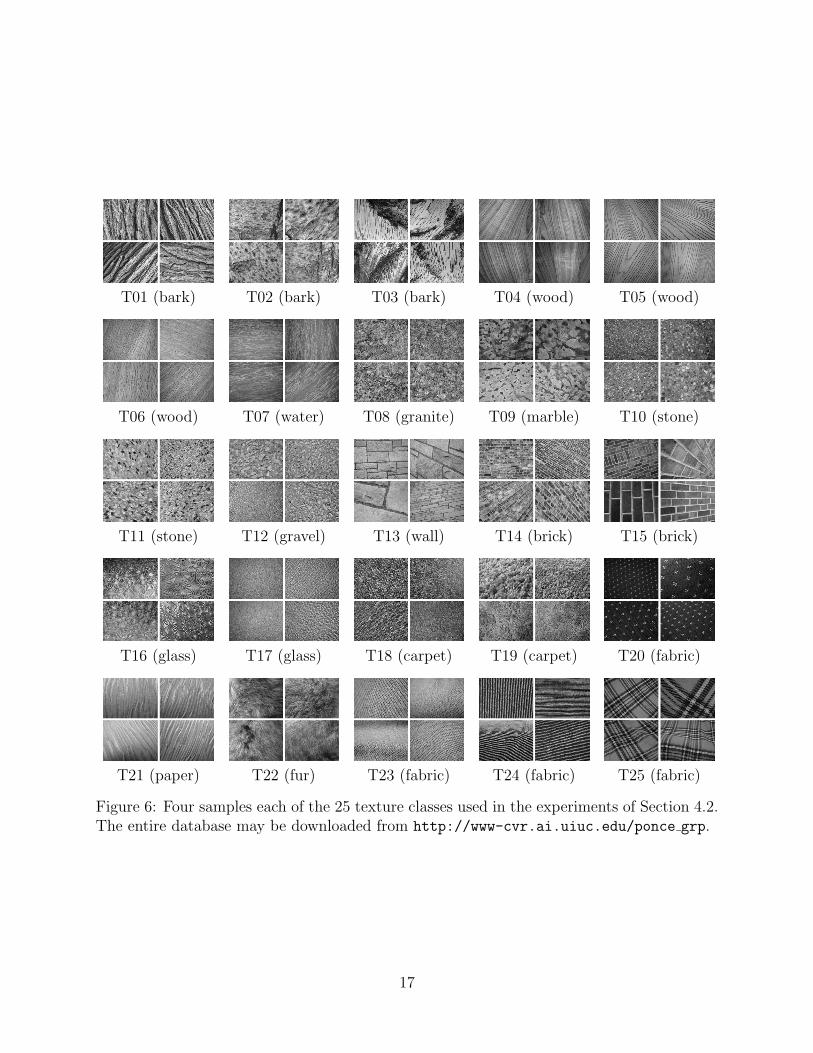
Figure 6 shows four sample images from each class (the resolution of the samples is 640×480

pixels). The database includes surfaces whose texture is due mainly to albedo variations (e.g.,

wood and marble), 3D shape (e.g., gravel and fur), as well as a mixture of both (e.g., carpet

and brick). Significant viewpoint changes and scale differences are present within each class,

and illumination conditions are uncontrolled. During data acquisition, we have taken care to

exercise additional sources of variability wherever possible. These include non-planarity of

the textured surface (bark), significant non-rigid deformations between different samples of

the same class (fur, fabric, and water), inhomogeneities of the texture pattern (bark, wood,

and marble), and viewpoint-dependent appearance variations (glass).

Each image in the database is processed with the Harris and Laplacian detectors. The

median number of Harris (resp. Laplacian) regions extracted per image is 926 (resp. 4591).

The median number of combined regions is 5553, or about 1.8% of the total number of

pixel locations in the image. Thus, we can see that the spatial selection performed by the

detectors results in a drastic compression of the amount of data that needs to be handled

by the subsequent processing stages, especially clustering, which is a notoriously memory-

intensive operation. In our implementation, clustering was performed using the k-means

algorithm with k = 40 centers.

16

T01 (bark) T02 (bark) T03 (bark) T04 (wood) T05 (wood)

T06 (wood) T07 (water) T08 (granite) T09 (marble) T10 (stone)

T11 (stone) T12 (gravel) T13 (wall) T14 (brick) T15 (brick)

T16 (glass) T17 (glass) T18 (carpet) T19 (carpet) T20 (fabric)

T21 (paper) T22 (fur) T23 (fabric) T24 (fabric) T25 (fabric)

Figure 6: Four samples each of the 25 texture classes used in the experiments of Section 4.2.The entire database may be downloaded from http://www-cvr.ai.uiuc.edu/ponce grp.

17

50 100 150 2000.4

0.5

0.6

0.7

0.8

0.9

Number of retrievals

Ave

. rec

all

HSHRH(S+R)

50 100 150 2000.4

0.5

0.6

0.7

0.8

0.9

Number of retrievals

Ave

. rec

all

LSLRL(S+R)

50 100 150 2000.4

0.5

0.6

0.7

0.8

0.9

Number of retrievals

Ave

. rec

all

(H+L)S(H+L)R(H+L)(S+R)

(a) (b) (c)

Figure 7: Retrieval curves for the texture database. (a) The Harris channels. (b) TheLaplacian channels. (c) The combined Harris and Laplacian channels.

Figure 7 shows retrieval results for the texture database. The first observation is that spin

images perform better than RIFT descriptors, and the combination of the two descriptors

performs slightly better than spin images alone. Next, Laplacian regions (part (b) of the

figure) perform better than Harris (a), and the combination of the two (c) is slightly better

than Laplacian alone. The solid curve in part (c) of the figure shows the retrieval performance

obtained by combining all four detector/descriptor channels. The recall after 39 retrievals is

58.92%. This relatively low number is a reflection of the considerable intra-class variability

of the database. As discussed in Section 4.1, we cannot expect that all samples of the same

class will be well represented by a single prototype. Accordingly, the combined (H+L)(S+R)

classification rate is only 62.15% for one training sample, but it goes up rapidly to 92.61% for

10 samples and 96.03% for 20 samples. Table 2 shows a comparison of 10-sample classification

rates for different channel combinations. The same trends that were seen in Figure 7 are

echoed here: Spin images perform better than RIFT, Laplacian regions perform better than

Harris, and the combination (H+L)(S+R) has the highest performance.

We may wonder whether the superior performance of Laplacian points is due to the denser

representation they afford (recall that the Laplacian detector finds almost five times as

many regions as the Harris). To check this conjecture, we have repeated the recognition

experiments after thresholding the output of the Laplacian detector so that equal numbers

of Laplacian and Harris regions are produced for each image. The results of the “truncated”

18

H L H+L

S 0.8332 0.8829 0.9015

R 0.7927 0.8318 0.8547

S+R 0.8814 0.9196 0.9261

Table 2: Classification results for 10 training samples per class. First column (top to bottom):HS, HR, H(S+R). Second column: LS, LR, L(S+R). Third column: (H+L)S, (H+L)R,(H+L)(S+R).

and “full” Laplacian representations may be compared by looking at columns 3 and 4 of

Table 3. Interestingly, while the rates may vary significantly for individual textures, the

averages (bottom row) are almost the same: 91.93% and 91.96% for “truncated” and “full”,

respectively. Thus, recognition performance cannot be regarded as a simple function of the

density of the representation.

Finally, Table 3 allows us to analyze the “difficulty” of individual textures for our sys-

tem. To this end, the textures are arranged in order of increasing (H+L)(S+R) classification

rate (last column). Roughly speaking, classification rate is positively correlated with the

homogeneity of the texture: Some of the lowest rates belong to inhomogeneous coarse-scale

textures like bark (T02, T03) and marble (T09), while some of the highest belong to homo-

geneous fine-scale textures like glass (T17), water (T07), and fabric (T20, T24). However,

this relationship is not universal. For example, granite (T08), which is fine-grained and

quite uniform, has a relatively low rate of 86.78%, while the large-scale, inhomogeneous wall

(T13) has a relatively high rate of 95.92%. It is also interesting (and somewhat unexpected)

that the performance of different classes does not depend on their nature as 3D or albedo

textures. Overall, the intrinsic characteristics of the various textures do not seem to provide

a clear pattern for predicting performance. This is not surprising if one keeps in mind that

classification performance is not related directly to intra-class variability, but to the extent

of separation between the classes in feature space.

19

Class H(S+R) L(S+R) (trunc.) L(S+R) (full) (H+L)(S+R)

T03 (bark) 0.7455 0.7248 0.7512 0.7953

T19 (carpet) 0.7270 0.8592 0.8207 0.8107

T02 (bark) 0.8077 0.8167 0.8018 0.8467

T08 (granite) 0.8352 0.8855 0.8808 0.8678

T09 (marble) 0.7515 0.8360 0.8950 0.8773

T21 (paper) 0.7445 0.9335 0.9230 0.8880

T16 (glass) 0.7610 0.9753 0.9367 0.8882

T12 (gravel) 0.7947 0.8703 0.9073 0.9012

T14 (brick) 0.8307 0.9048 0.8965 0.9028

T01 (bark) 0.8972 0.9295 0.8703 0.9063

T23 (fabric) 0.8898 0.9512 0.9082 0.9198

T15 (brick) 0.8987 0.9035 0.9067 0.9238

T11 (stone) 0.8920 0.9448 0.9488 0.9372

T05 (wood) 0.8983 0.8163 0.9250 0.9442

T10 (stone) 0.8500 0.9488 0.9687 0.9492

T22 (fur) 0.9453 0.9423 0.9208 0.9508

T25 (fabric) 0.9330 0.9590 0.9343 0.9590

T13 (wall) 0.9288 0.9508 0.9590 0.9592

T06 (wood) 0.9690 0.9535 0.9290 0.9743

T18 (carpet) 0.9660 0.9282 0.9800 0.9747

T04 (wood) 0.9868 0.9862 0.9618 0.9853

T20 (fabric) 0.9908 0.9702 0.9973 0.9948

T07 (water) 0.9980 0.9940 0.9905 0.9975

T24 (fabric) 0.9937 0.9990 0.9780 0.9980

T17 (glass) 1.0000 1.0000 0.9985 1.0000

Mean 0.8814 0.9193 0.9196 0.9261

Table 3: Detailed breakdown of classification results summarized in Table 2. The classes aresorted in order of increasing classification rate (last column). See text for discussion.

20

1 5 10 15 200

0.1

0.2

0.3

0.4

0.5

0.6

0.7

0.8

0.9

1

Number of training samples

Cla

ssifi

catio

n ra

te

maximummeanminimum

1 5 10 15 200

0.1

0.2

0.3

0.4

0.5

0.6

0.7

0.8

0.9

1

Number of training samples

Cla

ssifi

catio

n ra

te

maximummeanminimum

1 5 10 15 200

0.1

0.2

0.3

0.4

0.5

0.6

0.7

0.8

0.9

1

Number of training samples

Cla

ssifi

catio

n ra

te

maximummeanminimum

(a) (H+L)(S+R) (b) VZ-Joint (c) VZ-MRF

Figure 8: Comparative evaluation: Classification rate vs. number of training samples. Thehigher (dashed) curve shows the maximum classification rate achieved by any of the 25classes, the middle (solid) curve shows the mean, and the lower (dash-dot) curve shows theminimum. (a) Our method, (H+L)(S+R) combination. (b) VZ-Joint method. (c) VZ-MRFmethod.

Comparative evaluation. The results presented in this section clearly show that our lo-

cal affine-invariant representation is sufficient for the successful recognition of textures on

(possibly non-rigid) surfaces in three dimensions. To answer the question of whether its in-

variance properties are actually necessary, we have performed a comparative evaluation with

the non-invariant algorithm recently proposed by Varma and Zisserman [47]. This method,

dubbed VZ in the following, uses a dense set of 2D textons; the descriptors are raw pixel val-

ues measured in fixed-size neighborhoods (perhaps surprisingly, this feature representation

was found to outperform the more traditional filter banks). We chose the VZ method for

comparison because it achieves the best classification rates to date on the CUReT database

(up to 97.47%). We have tested two variants of VZ: In the first one, texture images are

described by one-dimensional texton histograms encoding the joint distribution of all pixel

values in the neighborhood; in the second, they are represented using two-dimensional his-

tograms that encode the conditional distribution of the center pixel given its neighborhood.

Accordingly, the respective variants are dubbed VZ-joint and VZ-MRF (for Markov Random

Field). The details of our implementation are given in the Appendix.

We have compared our method with with VZ-Joint and VZ-MRF using the randomized

classification scheme described in Section 4.1. Figure 8 shows the results as a function

of training set size. Consistent with the findings of Varma and Zisserman [47], VZ-MRF

21

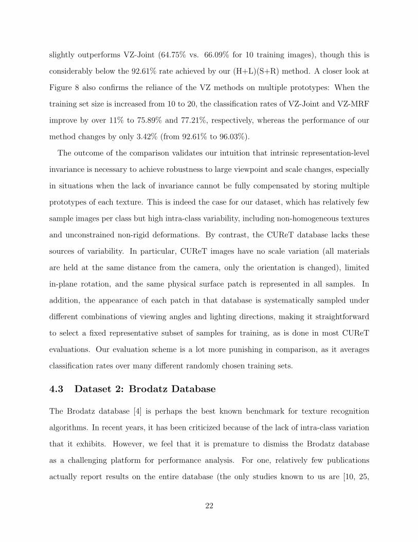
slightly outperforms VZ-Joint (64.75% vs. 66.09% for 10 training images), though this is

considerably below the 92.61% rate achieved by our (H+L)(S+R) method. A closer look at

Figure 8 also confirms the reliance of the VZ methods on multiple prototypes: When the

training set size is increased from 10 to 20, the classification rates of VZ-Joint and VZ-MRF

improve by over 11% to 75.89% and 77.21%, respectively, whereas the performance of our

method changes by only 3.42% (from 92.61% to 96.03%).

The outcome of the comparison validates our intuition that intrinsic representation-level

invariance is necessary to achieve robustness to large viewpoint and scale changes, especially

in situations when the lack of invariance cannot be fully compensated by storing multiple

prototypes of each texture. This is indeed the case for our dataset, which has relatively few

sample images per class but high intra-class variability, including non-homogeneous textures

and unconstrained non-rigid deformations. By contrast, the CUReT database lacks these

sources of variability. In particular, CUReT images have no scale variation (all materials

are held at the same distance from the camera, only the orientation is changed), limited

in-plane rotation, and the same physical surface patch is represented in all samples. In

addition, the appearance of each patch in that database is systematically sampled under

different combinations of viewing angles and lighting directions, making it straightforward

to select a fixed representative subset of samples for training, as is done in most CUReT

evaluations. Our evaluation scheme is a lot more punishing in comparison, as it averages

classification rates over many different randomly chosen training sets.

4.3 Dataset 2: Brodatz Database

The Brodatz database [4] is perhaps the best known benchmark for texture recognition

algorithms. In recent years, it has been criticized because of the lack of intra-class variation

that it exhibits. However, we feel that it is premature to dismiss the Brodatz database

as a challenging platform for performance analysis. For one, relatively few publications

actually report results on the entire database (the only studies known to us are [10, 25,

22

35, 50]). In addition, while near-perfect overall results have been shown for the CUReT

database [47], the best (to our knowledge) retrieval performance on the Brodatz database is

around 84% [50]. The reason for this is the impressive diversity of Brodatz textures, some

of which are quite perceptually similar, while others are so inhomogeneous that a human

observer would arguably be unable to group their samples “correctly”. The variety of the

scales and geometric patterns of the Brodatz textures, combined with an absence of intra-

class transformations, makes them a good platform for testing the discriminative power of

an additional local shape channel in a context where affine invariance is not necessary, as

described below.

The shape channel. The shape of an affinely adapted region is encoded in its local shape

matrix, which can also be thought of as the equation of an ellipse. Let E1 and E2 be two

ellipses in the image plane. We eliminate the translation between E1 and E2 by aligning

their centers, and then compute the dissimilarity between the regions as

d(E1, E2) = 1 − Area (E1 ∩ E2)

Area (E1 ∪ E2).

In the experiments of this section, we use local shape to obtain two additional channels,

HE and LE, corresponding to the ellipses found by the Harris and Laplacian detectors, re-

spectively. Notice that the ellipse ground distance, and consequently all shape-based EMD’s,

must be between 0 and 1. Because the descriptor-based EMD’s lie in the same range, the

shape-based EMD’s can be combined with them through simple addition.

Finally, it is worth noting that the ellipse “distance” as defined above takes into account

the relative orientations of the two ellipses. If it is necessary to achieve rotation invariance,

we can simply align the major and minor axes of the two ellipses before comparing their

areas.

Results. The Brodatz database consists of 111 images. Following the same procedure as

previous evaluations [25, 35, 50], we form classes by partitioning each image into nine non-

overlapping fragments, for a total of 999 images. Fragment resolution is 215 × 215 pixels.

23

10 20 30 40 50

0.45

0.55

0.65

0.75

0.85

0.95

Number of retrievals

Ave

. rec

all

HSHRH(S+R)

10 20 30 40 50

0.45

0.55

0.65

0.75

0.85

0.95

Number of retrievals

Ave

. rec

all

LSLRL(S+R)

10 20 30 40 50

0.45

0.55

0.65

0.75

0.85

0.95

Number of retrievals

Ave

. rec

all

(H+L)S(H+L)R(H+L)(S+R)

10 20 30 40 50

0.45

0.55

0.65

0.75

0.85

0.95

Number of retrievals

Ave

. rec

all

(H+L)E(H+L)(S+R)(H+L)(S+R+E)

(a) (b) (c) (d)

Figure 9: Retrieval curves for the Brodatz database. (a) Harris descriptor channels. (b)Laplacian descriptor channels. (c) Combined Harris and Laplacian descriptor channels. (d)Comparison of combined performance with and without the ellipse channels (HE and LE).

By comparison with the texture database discussed in the previous section, relatively few

regions are extracted from each image: The median values are 132 for the Harris detector,

681 for the Laplacian, 838 combined. Some images contain less than 50 regions total. Given

such small numbers, it is difficult to select a fixed number of clusters suitable for all im-

ages in the database. To cope with this problem, we replace k-means by an agglomerative

clustering algorithm that repeatedly merges clusters until the average intra-cluster distance

exceeds a specified threshold [17]. This process results in variable-sized signatures, which

are successfully handled by the EMD framework. An additional advantage of agglomerative

clustering as opposed to k-means is that it can be used for the shape channel, since it can

take as input the matrix of pairwise distances between the ellipses.

Figure 9 shows retrieval results for the Brodatz database. Similarly to the results of the

previous section, the Laplacian channels, shown in part (b) of the figure, have better perfor-

mance than the Harris channels, shown in part (a). Interestingly, though, for the Brodatz

database RIFT descriptors perform better than spin images — the opposite of what we have

found in Section 4.2. However, this discrepancy is due at least in part to the variability of

signature size (due to the use of agglomerative clustering) in the experimental setup of this

section. On average, the RIFT-based signatures of the Brodatz images have more clusters

than the spin-based signatures, and we conjecture that this raises the discriminative power

of the RIFT channel. Another interesting point is that combining the Harris and Lapla-

24

cian channels, as shown in (c), results in a slight drop of performance as compared to the

Laplacian channels alone. Finally, (d) shows the effect of adding the shape channels into the

mix. By themselves, these channels are relatively weak, since after 8 retrievals the (H+L)E

recall is only 44.59%. However, adding these channels to (H+L)(S+R) boosts the recall from

70.94% to 76.26%.

The trends noted above are also apparent in the classification results presented in Table 4.

By looking at the first two rows, we can easily confirm the relatively strong performance of

the RIFT descriptor (particularly for the Laplacian detector), as well as the marginal drop

in performance of the L+H channels as compared to L alone. The latter effect is also seen

in the last row of the table, where the (H+L)(S+R+E) classification rate is slightly inferior

to the L(S+R+E) rate.

H L H+L

S 0.6136 0.7570 0.7531

R 0.6000 0.8023 0.7640

E 0.3678 0.4932 0.5413

S+R+E 0.7761 0.8815 0.8744

Table 4: Brodatz database classification results for 3 training samples.

We can get a more detailed look at the performance of our system by examining Figure 10,

which shows a histogram of classification rates for all 111 classes using three training samples

per class. The histogram reveals that the majority of textures are highly distinguishable, and

only a few stragglers are located at the low end of the spectrum. In fact, 36 classes have 100%

classification rate, 49 classes have classification rate at least 99%, and 73 classes (almost two

thirds of the total number of classes) have rate at least 90%. The mean rate is 87.44%.

Figure 11 shows four textures that were classified successfully and four textures that were

classified unsuccessfully. Not surprisingly, the latter examples are highly non-homogeneous.

25

0.2 0.4 0.6 0.8 10

10

20

30

40

50

60

Classification rateN

umbe

r of

cla

sses

Figure 10: Histogram of classification rates for 3 training samples.

The best retrieval performance curve of our system, corresponding to the (H+L)(S+R+E)

combination, has 76.26% recall after 8 retrievals. This is a slightly higher than the results

reported in [25, 35], but below Xu et al. [50], who report 84% recall using the multiresolu-

tion simultaneous autoregressive (MRSAR) model. MRSAR models texture as a stationary

random field and uses a dense representation with fixed neighborhood shape and size. A

known shortcoming of MRSAR is its limited ability to measure perceptual similarity —

the method tends to confuse textures that appear very different to human observers [25].

Most significantly, the MRSAR model is difficult to extend with affine invariance. By con-

trast, our representation is specifically formulated with geometric invariance in mind, is

non-parametric, and does not make any statistical assumptions about the input texture.

Successes Failures

D48 D15 D94 D87 D30 D91 D45 D990.9708 0.9992 1.000 1.000 0.2242 0.2700 0.3417 0.3425

Figure 11: Left: successes. Right: failures. The average classification rates are shown belowthe corresponding class labels. Note that the representation for D48 has an average numberof only 27 combined Laplacian and Harris regions per sample.

26

5 Discussion

In this article, we have introduced a sparse affine-invariant texture representation that applies

spatial and shape selection to automatically determine the locations and support regions of

salient local texture regions. In summary, the main contributions of our work are:

• A sparse representation: The experiments of Section 4 show that it is possible to

successfully recognize many textures based on information contained in a very small

number of image regions.

• Spatial and shape selection: These mechanisms provide robustness against viewpoint

changes, non-rigid deformations, and non-homogeneity of the texture pattern. In ad-

dition, affine regions capture important perceptual characteristics of many textures.

• Novel intensity-based descriptors: Spin images and RIFT descriptors, presented in

Section 3.2, provide a high degree of invariance while serving as a rich description of

the intensity pattern of local texture patches.

• A flexible approach to invariance: Our system is flexible in that local shape information

may either be discarded or used as a feature, depending on the degree of invariance

required by the application.

In our experiments, we have evaluated two detectors and two descriptors on two datasets

of about a thousand images each. The first dataset has tested the invariance of our pro-

posed representation to viewpoint changes, as well as complex appearance changes and non-

rigid deformations. A comparative evaluation with the VZ method [47] has confirmed that

representation-level affine invariance is necessary for achieving good performance on a rela-

tively sparse dataset with high intra-class variability. However, it remains to be determined

whether the advantage of our method will persist when the training set can be made to

include representative samples of all variations that are likely to appear at testing time. In

this case, it is possible that our approach, which throws away potentially useful information

27

in the process of computing invariants, would prove less discriminative than an approach

based on multiple view-dependent prototypes. We plan to investigate this possibility in

future evaluations.

Our second set of experiments, carried out on the Brodatz database, has allowed us to test

the descriptive power of the local shape information captured by the affine region detectors.

As shown in Figure 9 (d), augmenting our model with an additional shape channel has

boosted the recall rate by almost 5%, from 70.94% to 76.26%. However, because these

results are still somewhat inferior to those reported by a non-invariant method [50], one

might wonder whether our strategy of factoring out shape in order to compute invariant

appearance descriptors, and then adding it back in as a separate “ellipse channel,” may

actually produce a less expressive model (at least, for this particular database) than an

approach that does not separate appearance and shape. Addressing this issue is another

interesting direction for further research.

Next, let us briefly summarize the findings of Section 4. The Laplacian detector has shown

better overall performance for both texture datasets; nevertheless, as can be seen from Table

3, the Harris detector can have superior performance for certain individual classes. The Har-

ris detector also has the advantage of producing much sparser image representations than

the Laplacian. As for descriptors, spin images won over RIFT for the texture database in

Section 4.2, while RIFT worked slightly better for the Brodatz database in Section 4.3 (how-

ever, recall that the latter comparison is confounded by signature size variability). Despite

these differences in performance, it is advantageous to retain both descriptors, as combining

their outputs generally improves the accuracy of recognition.

Perhaps the most important high-level observation we can make is that both the descrip-

tors and the detectors tend to fluctuate in performance from texture to texture and from

database to database. Two lessons can be drawn from this. On the one hand, researchers

working on specific applications of texture analysis should conduct comparative evaluations

on representative data to discover which channels or channel combinations would work best

28

in their case. On the other hand, to achieve a general understanding of the expressive

power of different channels on different types of texture, it is necessary to conduct system-

atic studies using much larger databases (containing hundreds or even thousands of texture

classes), as well as larger numbers of descriptors and detectors, or even parameterized descrip-

tor/detector families. Such studies should focus on quantifying performance as a function of

all sources of variability that may be of interest. Currently, our dataset includes some dimen-

sions, like non-rigidity of the surface and inhomogeneity of the texture pattern, that seem

difficult to quantify precisely. An important future research direction is the development

of systematic evaluation techniques suitable for dealing with large-scale datasets featuring

many degrees of freedom.

Another issue requiring further study is the method for combining channels. In our lim-

ited evaluation, the simple method of adding the individual EMD matrices has generally

proven effective in boosting performance. However, as we have learned from our Brodatz

experiments, it is occasionally possible for the combined recognition rate to actually be lower

than the single-channel rates. We plan to study more sophisticated methods for combining

channels that would not suffer from similar detrimental effects.

Finally, we plan to strengthen the proposed texture representation using spatial relation-

ships between neighboring regions. A few recent representations [28, 42] have used a two-level

scheme, with intensity-based textons at the first level and histograms of texton distributions

over local neighborhoods at the second level. For many natural textures, the arrangement of

affine regions captures perceptually important information about the global geometric struc-

ture. Augmenting our representation with such information is likely to increase its ability

to distinguish textures that have similar local neighborhoods but different spatial layouts.

To date, we have conducted preliminary experiments in classification of individual texture

regions using simple co-occurrence relations [20]. We expect that a richer two-level texture

representation will be useful for the problem of segmenting and classifying natural images

that contain multiple texture categories such as sky, water, plants, and man-made structures.

29

Appendix: Implementation of the VZ Method

At the feature extraction stage, all N × N pixel neighborhoods in an image are taken and

reordered to form N2-dimensional feature vectors. In our implementation, N = 11 for

121-dimensional features. This was selected as the smallest neighborhood size to yield a

feature space of higher dimensionality than spin images. To provide some invariance to

illumination changes, the vectors are normalized to zero mean and unit norm. To compute

the texton dictionary, five images per class are chosen at random, and 20% of all feature

vectors extracted from these images are retained, also at random. This reduction in the

number of feature vectors is motivated primarily by the memory limitations of our system.

The feature vectors for all 25 classes are clustered using k-means into 40 clusters each,

resulting in a dictionary of 1000 textons. For the VZ-joint variant, each pixel in an image is

labeled by its nearest texton center, and the distribution of all texton labels is represented

using a 1000-dimensional histogram. For the VZ-MRF variant, an image is represented using

a two-dimensional histogram: For each texton, a conditional distribution of the center pixel

is stored as a histogram with 20 bins. This gives us a 20, 000-dimensional representation

for each image. In both cases, histograms are compared using the χ2 distance, and nearest-

neighbor classification is used.

Acknowledgments

This research was partially supported by the National Science Foundation under grant IIS-

0308087, the European project LAVA (IST-2001-34405), the UIUC Campus Research Board,

the UIUC-CNRS collaboration agreement, and the Beckman Institute for Advanced Science

and Technology. We also wish to thank Andrew Zisserman and Manik Varma for many

useful discussions, and the anonymous reviewers for their constructive comments that have

helped us to improve this article.

30

References

[1] A. Baumberg. Reliable feature matching across widely separated views. In Proc. CVPR,

volume 1, pages 774–781, 2000.

[2] S. Belongie, J. Malik, and J. Puzicha. Shape matching and object recognition using

shape contexts. IEEE Trans. PAMI, 24(4):509–522, 2002.

[3] D. Blostein and N. Ahuja. A multiscale region detector. Computer Vision, Graphics

and Image Processing, 45:22–41, 1989.

[4] P. Brodatz. Textures: A Photographic Album for Artists and Designers. Dover, New

York, 1966.

[5] F.S. Cohen, Z. Fan, and M.A.S. Patel. Classification of rotated and scaled textured

images using Gaussian Markov field models. IEEE Trans. PAMI, 13(2):192–202, 1991.

[6] J.L Crowley and A.C. Parker. A representation of shape based on peaks and ridges in

the difference of low-pass transform. IEEE Trans. PAMI, 6:156–170, 1984.

[7] O.G. Cula and K.J. Dana. Compact representation of bidirectional texture functions.

In Proc. CVPR, volume 1, pages 1041–1047, 2001.

[8] K.J. Dana, B. van Ginneken, S.K. Nayar, and J.J. Koenderink. Reflectance and texture

of real world surfaces. ACM Transactions on Graphics, 18(1):1–34, 1999.

[9] J. Garding and T. Lindeberg. Direct computation of shape cues using scale-adapted

spatial derivative operators. IJCV, 17(2):163–191, 1996.

[10] B. Georgescu, I. Shimshoni, and P. Meer. Mean shift based clustering in high dimensions:

A texture classification example. In Proc. ICCV, pages 456–463, 2003.

[11] R. Haralick. Statistical and structural approaches to texture. Proceedings of the IEEE,

67:786–804, 1979.

31

[12] C. Harris and M. Stephens. A combined corner and edge detector. In M. M. Matthews,

editor, Proceedings of the 4th Alvey Vision Conference, pages 147–151, 1988.

[13] A. Johnson and M. Hebert. Using spin images for efficient object recognition in cluttered

3d scenes. IEEE Trans. PAMI, 21(5):433–449, 1999.

[14] B. Julesz. Visual pattern discrimination. IRE Transactions on Information Theory,

IT-8:84–92, 1962.

[15] B. Julesz. Textons, the elements of texture perception and their interactions. Nature,

290:91–97, 1981.

[16] T. Kadir and M. Brady. Scale, saliency and image description. IJCV, 45(2):83–105,

2001.

[17] L. Kaufman and P. Rousseeuw. Finding Groups in Data: An Introduction to Cluster

Analysis. John Wiley & Sons, New York, 1990.

[18] J. Koenderink and A. Van Doorn. Representation of local geometry in the visual system.

Biological Cybernetics, 55:367–375, 1987.

[19] J. Koenderink and A. Van Doorn. The structure of locally orderless images. IJCV,

31(2/3):159–168, 1999.

[20] S. Lazebnik, C. Schmid, and J. Ponce. Affine-invariant local descriptors and neighbor-

hood statistics for texture recognition. In Proc. ICCV, pages 649–655, 2003.

[21] S. Lazebnik, C. Schmid, and J. Ponce. A sparse texture representation using affine-

invariant regions. In Proc. CVPR, volume 2, pages 319–324, 2003.

[22] T. Leung and J. Malik. Recognizing surfaces using three-dimensional textons. IJCV,

43(1):29–44, 2001.

32

[23] E. Levina and P. Bickel. The Earth Mover’s distance is the Mallows distance: Some

insights from statistics. In Proc. ICCV, volume 2, pages 251–256, 2001.

[24] T. Lindeberg. Feature detection with automatic scale selection. IJCV, 30(2):77–116,

1998.

[25] F. Liu and R. W. Picard. Periodicity, directionality, and randomness: Wold features for

image modeling and retrieval. IEEE Trans. PAMI, 18(7):722–733, 1996.

[26] X. Llado, J. Marti, and M. Petrou. Classification of textures seen from different dis-

tances and under varying illumination direction. In IEEE Int. Conf. Image Processing,

volume 1, pages 833–836, 2003.

[27] D. Lowe. Distinctive image features from scale-invariant keypoints. IJCV, 60(2):91–110,

2004.

[28] J. Malik, S. Belongie, T. Leung, and J. Shi. Contour and texture analysis for image

segmentation. IJCV, 43(1):7–27, 2001.

[29] J. Malik and P. Perona. Preattentive texture discrimination with early vision mecha-

nisms. J. Opt. Soc. Am. A, 7(5):923–932, 1990.

[30] J. Mao and A. Jain. Texture classification and segmentation using multiresolution

simultaneous autoregressive models. Pattern Recognition, 25:173–188, 1992.

[31] J. Matas, O. Chum, U. Martin, and T Pajdla. Robust wide baseline stereo from maxi-

mally stable extremal regions. In Proc. BMVC, volume 1, pages 384–393, 2002.

[32] K. Mikolajczyk and C. Schmid. Indexing based on scale invariant interest points. In

Proc. ICCV, pages 525–531, 2001.

[33] K. Mikolajczyk and C. Schmid. An affine invariant interest point detector. In Proc.

ECCV, volume 1, pages 128–142, 2002.

33

[34] K. Mikolajczyk and C. Schmid. A performance evaluation of local descriptors. In Proc.

CVPR, volume 2, pages 257–263, 2003.

[35] R. Picard, T. Kabir, and F. Liu. Real-time recognition with the entire Brodatz texture

database. In Proc. CVPR, pages 638–639, 1993.

[36] J. Puzicha, Y. Rubner, C. Tomasi, and J. Buhmann. Empirical evaluation of dissim-

ilarity measures for color and texture. In Proc. ICCV, volume 2, pages 1165–1172,

1999.

[37] T. Randen and J. Husøy. Filtering for texture classification: A comparative study. IEEE

Trans. PAMI, 21(4):291–310, 1999.

[38] Y. Rubner and C. Tomasi. Texture-based image retrieval without segmentation. In

Proc. ICCV, pages 1018–1024, 1999.

[39] Y. Rubner, C. Tomasi, and L. Guibas. The Earth Mover’s distance as a metric for

image retrieval. IJCV, 40(2):99–121, 2000.

[40] F. Schaffalitzky and A. Zisserman. Viewpoint invariant texture matching and wide

baseline stereo. In Proc. ICCV, volume 2, pages 636–643, 2001.

[41] F. Schaffalitzky and A. Zisserman. Multi-view matching for unordered image sets, or

“How do I organize my holiday snaps?”. In Proc. ECCV, volume 1, pages 414–431,

2002.

[42] C. Schmid. Constructing models for content-based image retrieval. In Proc. CVPR,

volume 2, pages 39–45, 2001.

[43] C. Schmid and R. Mohr. Local greyvalue invariants for image retrieval. IEEE Trans.

PAMI, 19(5):530–535, 1997.

34

[44] J. Sivic and A. Zisserman. Video Google: A text retrieval approach to object matching

in videos. In Proc. ICCV, pages 1470–1477, 2003.

[45] T. Tuytelaars and L. Van Gool. Matching widely separated views based on affinely

invariant neighbourhoods. IJCV, 59(1):61–85, 2004.

[46] M. Varma and A. Zisserman. Classifying images of materials: Achieving viewpoint and

illumination independence. In Proc. ECCV, volume 3, pages 255–271, 2002.

[47] M. Varma and A. Zisserman. Texture classification: Are filter banks necessary? In

Proc. CVPR, volume 2, pages 691–698, 2003.

[48] H. Voorhees and T. Poggio. Detecting textons and texture boundaries in natural images.

In Proc. ICCV, pages 250–258, 1987.

[49] J. Wu and M. J. Chantler. Combining gradient and albedo data for rotation invariant

classification of 3d surface texture. In Proc. ICCV, volume 2, pages 848–855, 2003.

[50] K. Xu, B. Georgescu, D. Comaniciu, and P. Meer. Performance analysis in content-based

retrieval with textures. In Proc. Int. Conf. Patt. Recog., volume 4, pages 275–278, 2000.

[51] J. Zhang, P. Fieguth, and D. Wang. Random field models. In A. Bovik, editor, Handbook

of Image and Video Processing, pages 301–312. Academic Press, San Diego, CA, 2000.

35