Embed Size (px)
Citation preview

Universita degli studi“Roma Tre”
Facolta di Ingegneria
Corso di Laurea Magistrale in Ingegneria Informatica
A SPARQL front-end for MonetDB
Relatore Correlatore Laureando
Paolo Atzeni Peter A. Boncz Marco Antonelli
274455
Anno Accademico 2007/2008

Preface
This thesis starts with a collaboration with the CWI, Center forMathematics andInformatics (in Dutch: Centrum voor Wiskunde en Informatica), a prestigiousDutch research center located in Amsterdam, one of the most important in Europein these fields and a member of the ERCIM, the European Research Consortiumfor Informatics and Mathematics.
One of the research themes at the CWI concerns the problems relative to the“data explosion”: how to find relevant information in the increasing amount of theavailable data?
On this theme one of the research groups of the CWI has been developingsince 1994 MonetDB, an open-source database management system specialized inobtaining high performances in query-intensive applications like decision support(OLAP), data mining, geographical information systems (GIS) and XQuery; thisDBMS is and has been since its early stages a scientific research platform in thedatabase field.
A new application of relational systems is RDF data storage and query; thegoal of this language is to formally express metadata in asubject-predicate-objectform, making the information that this language describes intelligible to a com-puter. A web page is now comprehensible only to humans; but ifthe meaning ofthat page is expressed in a formal language then it can be automatically processedmaking content search, for instance, much more effective. RDF constitute thusthe foundations of the web of the future, the “Semantic Web”.
How relational engines can manage and query effectively considerable amoun-ts of RDF triples, in the order of hundreds of millions, is still the object of aremarkable scientific research effort.
My job at CWI was to kick-start the MonetDB front/end for SPARQL, theRDF query language.
The developed code, in C language, brought on one side to the creation ofa new module of MonetDB, described in chapter 5, that defines the relationalstructures that contain the RDF data and the import and exportfunctions from andto plain textual documents; on the other to a SPARQL parser which, given a query,it translates it to its algebraic form.
i

PREFACE ii
The theoretical work concerned the translation of the SPARQLalgebra inrelational algebra, proposed in the last section of chapter4.
The first chapter describes RDF, both in its syntax and its semantics; chapter2 introduces MonetDB, its fundamental principles, its architecture and the datastructure on which this DBMS is centered on, the binary table.
Chapter 3 illustrates the general RDF storage techniques and gives an over-view of the main projects related to this subject.
Chapter 4 exposes, in examples and formally, the SPARQL query languageand its algebra; the last section, referref to above, proposes for each operator ofthis algebra an equivalent relational expression.
The last chapter describes the data structures used in MonetDB to containthe RDF triples, how these are imported from a textual document, and which areadvantages and drawbacks of the suggested solution.
Appendix A, finally, examines a set of choices that MonetDB/SPARQL mayperform to get the maximum benefit from the adopted data structures.

Prefazione
Questa tesi nasce da un esperienza di lavoro presso il CWI, Centro per la Mate-matica e l’Informatica (in olandese: Centrum voor Wiskunde en Informatica), unprestigioso centro di ricerca olandese situato ad Amsterdam, uno dei piu impor-tanti in Europa in questi campi e membro dell’ERCIM, il consorzio europeo perl’Informatica e la Matematica, di cui fa parte anche il CNR italiano.
Una delle tematiche di ricerca scientifica presso il CWI riguarda le problema-tiche relative alla “esplosione dei dati”: come trovare informazioni rilevanti nellasempre crescente quantita di informazioni disponibili?
In quest’ambito uno dei gruppo di ricerca del CWI sviluppa sin dal 1994 Mo-netDB, un DBMS open-source specializzato per ottenere alte prestazioni in appli-cazioni “query-intensive” come il supporto decisionale (OLAP), il data mining, isistemi informativi geografici (GIS) e XQuery; questo DBMSe ede stato per tuttiquesti anni una piattaforma per la ricerca scientifica nel campo delle basi di dati.
Una nuova applicazione dei sistemi relazionali consiste nell’immagazzina-mento e la ricerca di dati espressi in RDF; lo scopo di questo linguaggioe di espri-mere in maniera formale dei metadati sotto forma di triplesoggetto-predicato-oggetto, rendendo in tal modo intellegibile per un calcolatore le informazioni chequesto linguaggio descrive. Una pagina web, oggi,e comprensibile solo ad unessere umano; ma se le informazioni contenute sono espressein un linguaggioformale allora queste possono essere processate automaticamente rendendo le ri-cerche di contenuti, ad esempio, molto piu efficaci. RDF costituisce dunque lefondamenta del web del futuro, il “Web Semantico”.
Come possano pero riuscire i sistemi relazionali a contenere ed interroga-re efficacemente quantita considerevoli di triple RDF, dell’ordine di centinaia dimilioni, e ancora oggetto di un notevole sforzo di ricerca.
Il mio compito presso il CWIe stato quello di iniziare il front/end di MonetDBper SPARQL, il linguaggio di interrogazione per RDF.
Lo sviluppo di codice, in linguaggio C, ha portato da una partealla creazionedi un nuovo modulo di MonetDB, descritto nel capitolo 5, che definisce le strutturerelazionali per la rappresentazione dei dati RDF e le funzioni di importazione ed
iii

PREFAZIONE iv
esportazione di documenti in forma testuale; dall’altra adun parser per SPARQL,che data una query la traduce nella sua forma algebrica.
Il lavoro teorico ha riguardato la traduzione dell’algebraSPARQL in algebrarelazionale, proposta nell’ultima sezione del 4° capitolo.
Il 1° capitolo della tesi descrive RDF, sia nella sintassi chenella semantica; ilsecondo mentre il 2° introduce MonetDB, i sui principi basilari, la sua architetturae la struttura dati sulla quale questo DBMSe incentrato, la tabella binaria.
Il capitolo 3 illustra le tecniche generali di immagazzinamento di RDF edeffettua una panoramica dei principali progetti correlati a questo argomento.
Il quarto capitolo espone sia per esempi sia formalmente il linguaggio di inter-rogazione SPARQL e la sua algebra; l’ultima sezione, come detto sopra, proponeper ogni operatore di quest’algebra una espressione relazionale equivalente.
L’ultimo capitolo descrive le strutture dati utilizzate inMonetDB progettateper contenere le triple RDF, come queste vengano importante da un documentotestuale, e quali siano i vantaggi e gli svantaggi della soluzione proposta.
L’Appendice A, infine, esamina un insieme di scelte che MonetDB/SPARQLpuo intraprendere per trarre il massimo vantaggio dalle strutture dati utlizzate.
Contents
Preface i
Prefazione iii
1 The Resource Description Framework 11.1 Introduction . . . . . . . . . . . . . . . . . . . . . . . . . . . . . 11.2 Uniform Resource Identifiers . . . . . . . . . . . . . . . . . . . . 11.3 Graph Data Model . . . . . . . . . . . . . . . . . . . . . . . . . 21.4 RDF serialization languages . . . . . . . . . . . . . . . . . . . . 3
1.4.1 Notation3, Turtle and N-Triples . . . . . . . . . . . . . . 31.4.2 URI namespaces used in this thesis . . . . . . . . . . . . 41.4.3 RDF/XML . . . . . . . . . . . . . . . . . . . . . . . . . 4
1.5 Blank nodes . . . . . . . . . . . . . . . . . . . . . . . . . . . . . 51.6 Literals . . . . . . . . . . . . . . . . . . . . . . . . . . . . . . . 6
1.6.1 Datatypes . . . . . . . . . . . . . . . . . . . . . . . . . . 61.6.2 Typed literals . . . . . . . . . . . . . . . . . . . . . . . . 61.6.3 Plain literals . . . . . . . . . . . . . . . . . . . . . . . . 7
1.7 RDF Schema . . . . . . . . . . . . . . . . . . . . . . . . . . . . 71.7.1 Classes . . . . . . . . . . . . . . . . . . . . . . . . . . . 81.7.2 Properties . . . . . . . . . . . . . . . . . . . . . . . . . . 81.7.3 Richer schema languages . . . . . . . . . . . . . . . . . . 10
2 MonetDB 112.1 Design principles . . . . . . . . . . . . . . . . . . . . . . . . . . 11
2.1.1 A simple binary algebra . . . . . . . . . . . . . . . . . . 112.1.2 Main memory DBMS . . . . . . . . . . . . . . . . . . . 12
2.2 Architecture overview . . . . . . . . . . . . . . . . . . . . . . . . 132.3 Binary tables structure . . . . . . . . . . . . . . . . . . . . . . . 142.4 Binary table optimizations . . . . . . . . . . . . . . . . . . . . . 162.5 Current status and future . . . . . . . . . . . . . . . . . . . . . . 17
v

CONTENTS vi
3 RDF storage techniques and related work 193.1 RDF storage techniques . . . . . . . . . . . . . . . . . . . . . . . 193.2 OpenLink Virtuoso . . . . . . . . . . . . . . . . . . . . . . . . . 22
3.2.1 Main table indexing . . . . . . . . . . . . . . . . . . . . 233.2.2 Query optimization through data sampling . . . . . . . . . 23
3.3 Sesame . . . . . . . . . . . . . . . . . . . . . . . . . . . . . . . 243.3.1 Architecture of Sesame . . . . . . . . . . . . . . . . . . . 243.3.2 SAIL . . . . . . . . . . . . . . . . . . . . . . . . . . . . 24
3.4 Jena . . . . . . . . . . . . . . . . . . . . . . . . . . . . . . . . . 273.4.1 Storage schema . . . . . . . . . . . . . . . . . . . . . . . 273.4.2 Architecture . . . . . . . . . . . . . . . . . . . . . . . . . 28
3.5 Other storage engines . . . . . . . . . . . . . . . . . . . . . . . . 29
4 SPARQL 314.1 Introduction . . . . . . . . . . . . . . . . . . . . . . . . . . . . . 314.2 Graph Patterns . . . . . . . . . . . . . . . . . . . . . . . . . . . 31
4.2.1 Basic Graph Patterns . . . . . . . . . . . . . . . . . . . . 324.2.2 Group Graph Patterns . . . . . . . . . . . . . . . . . . . 334.2.3 Optional Graph Patterns . . . . . . . . . . . . . . . . . . 344.2.4 Union Graph Patterns . . . . . . . . . . . . . . . . . . . . 354.2.5 Filtering results . . . . . . . . . . . . . . . . . . . . . . . 36
4.3 RDF Datasets . . . . . . . . . . . . . . . . . . . . . . . . . . . . 364.3.1 Patterns on Named Graphs . . . . . . . . . . . . . . . . . 38
4.4 SPARQL semantics . . . . . . . . . . . . . . . . . . . . . . . . . 404.4.1 Initial definitions . . . . . . . . . . . . . . . . . . . . . . 404.4.2 SPARQL abstract query . . . . . . . . . . . . . . . . . . 424.4.3 Graph Pattern translation to SPARQL algebra . . . . . . . 434.4.4 Modifiers translation to SPARQL algebra . . . . . . . . . 454.4.5 Basic Graph Patterns . . . . . . . . . . . . . . . . . . . . 454.4.6 SPARQL algebra . . . . . . . . . . . . . . . . . . . . . . 464.4.7 Expression Evaluation . . . . . . . . . . . . . . . . . . . 49
4.5 SPARQL to Relational Algebra translation . . . . . . . . . . . . . 504.5.1 Relational algebra on multisets . . . . . . . . . . . . . . . 504.5.2 Filter translation . . . . . . . . . . . . . . . . . . . . . . 544.5.3 BGP translation . . . . . . . . . . . . . . . . . . . . . . . 544.5.4 Join translation . . . . . . . . . . . . . . . . . . . . . . . 554.5.5 LeftJoin translation . . . . . . . . . . . . . . . . . . . . . 574.5.6 Union translation . . . . . . . . . . . . . . . . . . . . . . 584.5.7 Graph expression translation . . . . . . . . . . . . . . . . 59

CONTENTS vii
5 RDF storage in MonetDB 605.1 Data structures . . . . . . . . . . . . . . . . . . . . . . . . . . . 60
5.1.1 Data tables . . . . . . . . . . . . . . . . . . . . . . . . . 605.1.2 Dictionary table . . . . . . . . . . . . . . . . . . . . . . . 60
5.2 Importing algorithm . . . . . . . . . . . . . . . . . . . . . . . . . 675.2.1 First phase . . . . . . . . . . . . . . . . . . . . . . . . . 685.2.2 Second phase – sorting . . . . . . . . . . . . . . . . . . . 69
5.3 Conclusions . . . . . . . . . . . . . . . . . . . . . . . . . . . . . 70
Appendices 74
A Materialized view choice 74A.1 Single triple pattern BGPs . . . . . . . . . . . . . . . . . . . . . 74
A.1.1 3 variables . . . . . . . . . . . . . . . . . . . . . . . . . 74A.1.2 2 variables . . . . . . . . . . . . . . . . . . . . . . . . . 75A.1.3 1 variable . . . . . . . . . . . . . . . . . . . . . . . . . . 75
A.2 BGPs of two triple patterns . . . . . . . . . . . . . . . . . . . . . 76A.2.1 No constraints . . . . . . . . . . . . . . . . . . . . . . . 76A.2.2 1 constraint . . . . . . . . . . . . . . . . . . . . . . . . . 77A.2.3 2 constraints . . . . . . . . . . . . . . . . . . . . . . . . 79A.2.4 3 constraints . . . . . . . . . . . . . . . . . . . . . . . . 81A.2.5 4 constraints . . . . . . . . . . . . . . . . . . . . . . . . 83
A.3 More complex BGP examples . . . . . . . . . . . . . . . . . . . 83A.3.1 Query 1 . . . . . . . . . . . . . . . . . . . . . . . . . . . 83A.3.2 Query 2 . . . . . . . . . . . . . . . . . . . . . . . . . . . 84A.3.3 Query 3 . . . . . . . . . . . . . . . . . . . . . . . . . . . 85

Chapter 1
The Resource DescriptionFramework
1.1 Introduction
The Resource Description Framework [5] is “a language for representing infor-mation about resources in the World Wide Web” [38].
RDF is based on the idea that each piece of information is a resource thathas properties that have values. The resources can be described, therefore, by aset ofstatementsin the subject-predicate-object format: thesubjectis that partof the statement that identifies the Web resource under description, thepredicateidentifies a property of the subject, and theobject is the value of that property.Because all statements have this structure, they are also called triples.
A statement with this simple subject-predicate-object structure may be
The page http://example.org/index.html has a creator whose value is John Smith
wherehttp://example.org/index.html is the subject,creator is the predicateandJohn Smith is the object.
1.2 Uniform Resource Identifiers
The above example, however, does not unequivocally identify what the conceptof creator or who John Smith is. Any resource, that might be a web page, abook, a person, or any abstract concept has to be described byan Uniform Re-source Identifieror URI. URIs are a generalization of URLs (Uniform ResourceLocators), that identify a resource by its access mechanism. URL are well suitedfor web pages or mail boxes, but not for any other resource that is not physicallyaccessible on the Web.
1

CHAPTER 1. THE RESOURCE DESCRIPTION FRAMEWORK 2
The above statement may be represented by an RDF triple having:
• a subjecthttp://example.org/index.html
• a predicatehttp://purl.org/dc/elements/1.1/creator
• an objecthttp://example.org/staffid/85740
wherehttp://purl.org/dc/elements/1.1/creator is a URI that identifies the“creator” concept, andhttp://example.org/staffid/85740 unequivocally identi-fies a specific John Smith.
A further generalization of URIs areIRIs, i.e. Internationalized ResourceIdentifiers, that are not restricted to the ASCII character set but allow also Uni-code characters. Every URI is also an IRI, and every IRI can be translated to anURI, substituting every non-ASCII character with the equivalent “percent encod-ing”, that consists of a ‘%’ followed by the Unicode codepoint that identifies thecharacter.
1.3 Graph Data Model
Since the object of an RDF statement may be a subject of anothertriple, a setof statement forms a labeled and directed graph, where subjects and objects arenodes and each predicate is an edge directed from a subject toan object.
Figure 1.1 is a simple RDF graph that extends the above example.
http://example.org/staffid/85740
John Smith mailto://[email protected]
http://example.org/index.html
http://purl.org/dc/elements/1.1/creator
http://example.org/terms/name
http://example.org/mailbox
Figure 1.1: Simple RDF graph

CHAPTER 1. THE RESOURCE DESCRIPTION FRAMEWORK 3
The URI http://example.org/staffid/85740 has two additional properties:the name of the person represented by the URI and his mailbox. As figure 1.1may suggest, object can be either URIs or constant values, called literals. In thefigure, literals are shown as boxes, and URIs as ellipses.
1.4 RDF serialization languages
This section introduces the languages to express RDF data in plain text files. It isnot intended to be a complete reference, but just an introduction needed to showexample data in a rigorous manner; many details will be skipped for the momentand introduced later in this chapter, when necessary.
The recommended standard language is RDF/XML [13], that encodes thetriples in the tree structure of XML. Since it is not easily readable for humans,the Notation3 (or N3) [15] language has been developed: the approach of N3 andits dialects, Turtle [14] and N-Triples [29], is to explicitly list the RDF statementsone after the other.
1.4.1 Notation3, Turtle and N-Triples
These languages are each a subset of the other, with Notation3 being the largestand N-Triples the smallest; for this reason, and because of the total compatibil-ity of the smaller languages with the larger ones, N3, Turtleand N-Triples aredescribed together.
Each statement of an RDF graph is listed on a different line, terminated by adot. The subject, the predicate and the object are separatedby white spaces, theURIs are written between ‘<’ and ‘>’ characters and the literals are quoted.
The RDF graph in figure 1.1 can expressed with
<http://example.org/index.html> <http://purl.org/dc/elements/1.1/creator> <http://example.org/staffid/85740> .
<http://example.org/staffid/85740> <http://example.org/terms/name> "John Smith" .
<http://example.org/staffid/85740> <http://example.org/terms/mailbox> <mailto://[email protected]> .
or more compactly, in Turtle and N3, with
@prefix ex: <http://example.org/> .
@prefix exterms: <http://example.org/terms/> .
@prefix exstaff: <http://example.org/staffid/> .
@prefix dc: <http://purl.org/dc/elements/1.1/> .
ex:index.html dc:creator exstaff:85740 .
exstaff:85740 exterms:name "John Smith" .
exstaff:85740 exterms:mailbox <mailto://[email protected]> .
N3 and Turtle permit one to declare URI prefixes, while N-Triples does notallow it. This language, in fact, was intended as a test-caselanguage, and thusN-Triples documents were not supposed to be written or read by humans.

CHAPTER 1. THE RESOURCE DESCRIPTION FRAMEWORK 4
A URI reference can thus be expressed in N3 and Turtle with aqualified name,that consists of a prefix that has been assigned to a namespaceURI, a colon anda local name, without angle brackets. The full URI reference is the concatenationof the namespace associated with the prefix and the local name.
1.4.2 URI namespaces used in this thesis
From now on, this thesis will make use of the following “well-known” prefixes tokeep URI references short and to avoid repetition:
@prefix rdf: http://www.w3.org/1999/02/22-rdf-syntax-ns#
@prefix rdfs: http://www.w3.org/2000/01/rdf-schema#
@prefix dc: http://purl.org/dc/elements/1.1/
@prefix xsd: http://www.w3.org/2001/XMLSchema#
1.4.3 RDF/XML
RDF/XML [13] is the recommended serialization language for RDF, but since N3and its subsets are easier to read, their use will be preferred for the examples ofthis thesis.
The graph in figure 1.1 in RDF/XML can be expressed as:
<?xml version="1.0"?>
<!DOCTYPE rdf:RDF [
<!ENTITY rdf "http://www.w3.org/1999/02/22-rdf-syntax-ns#">
<!ENTITY ex "http://example.org/">
<!ENTITY exstaff "http://example.org/staffid/">
<!ENTITY exterms "http://example.org/terms/">
<!ENTITY dc "http://purl.org/dc/elements/1.1/">
]>
<rdf:RDF xmlns:rdf = "&rdf;"
xmlns:exterms = "&exterms;"
xmlns:dc = "&dc;">
<rdf:Description rdf:about="&ex;index.html">
<dc:creator rdf:resource="&exstaff;85740"/>
</rdf:Description>
<rdf:Description rdf:about="&exstaff;85740">
<exterms:name>John Smith</exterms:name>
<exterms:mailbox rdf:resource="mailto://[email protected]"/>
</rdf:Description>
</rdf:RDF>
The ENTITY declarations are shorthand: the string associated with theentityrdf can be referenced further in the document by&rdf; . The names of the tagsare qualified names, and are expanded as in N3; the prefix in this case is declaredas an XML namespace (i.e.xmlns ).

CHAPTER 1. THE RESOURCE DESCRIPTION FRAMEWORK 5
The URI references of a subject of a statement are generally declared in therdf:about attribute of anrdf:Description tag, whose internal nodes represent theproperties of that subject and their values.
1.5 Blank nodes
Other kinds of nodes that can be found in RDF graphs, together with URI ref-erences and literals, are blank nodes. These, unlike literals and like the URIrefscan be both subject and objects, but with the difference that they do not have auniversal name; blank nodes are therefore local to an RDF graph.
Blank nodes are frequently used to encapsulate structured data, as shown infigure 1.2 for an address.
England34
Royal College St. London
http://example.org/staffid/85740
http://example.org/terms/housenumber http://example.org/terms/state
http://example.org/terms/street
http://example.org/terms/city
http://example.org/terms/address
Figure 1.2: A blank node representing an address
In N3 a blank node is represented by a blank node identifier. Two identical idsin a graph refer to the same blank node, but equal identifiers in different graphsrefer to different nodes, since separate graphs do not share any of them.
The graph in figure 1.2 can be expressed in N3 as
@prefix exstaff: http://example.org/staffid/
@prefix exterms: http://example.org/terms/
exstaff:85740 exterms:address _:address .
_:address exterms:housenumber "34" .
_:address exterms:street "Royal College St." .
_:address exterms:city "London" .
_:address exterms:state "England" .
Blank node identifiers start with an underscore and a colon, followed by alabel: in the example:address is the identifier of the blank node that representsthe address.

CHAPTER 1. THE RESOURCE DESCRIPTION FRAMEWORK 6
1.6 Literals
The literals presented heretofore this section were untyped, just sequences of char-acters. Using the RDF terminology they areplain literals. RDF permits alsotypedliterals, were the type is identified by a URI reference.
Since XML Schema already defines a complete type system [16],RDF doesnot define any new type except one,rdf:XMLLiteral , used for embedding XMLin RDF.
1.6.1 Datatypes
Formally, a datatype consists of a lexical space, a value space and a lexical-to-value mapping.
The XML boolean datatypexsd:boolean , for example, has a value space oftwo elements:
V =
T, F
.
a lexical space of four elements:
L =
“true”, “false”, “1”, “0”
.
and the following lexical-to-value mapping:
M =
<“true”, T>, <“1”, T>, <“0”, F>, <“false”, F>
.
1.6.2 Typed literals
The general way to express a typed literal in the Notation3 dialects is:
"[Lexical Form]"ˆˆ<[URI reference]>
and only in N3 and Turtle:
"[Lexical Form]"ˆˆ[Qualified name]
The integer 24 is thus"24"ˆˆ<http://www.w3.org/2001/XMLSchema#integer> or"24"ˆˆxsd:integer . N3 and Turtle can also parse numeric and boolean literalswith no datatype URI and cast them automatically. The constant value true ,with no quotes, is equivalent to"true"ˆˆxsd:boolean , and123 is equivalent to123ˆˆxsd:integer .

CHAPTER 1. THE RESOURCE DESCRIPTION FRAMEWORK 7
XML literals
XML literals are literals whose value space is an XML tree. InRDF/XML docu-ments, custom XML markups can be embedded with therdf:parseType="Literal"
attribute:
<?xml version="1.0"?>
<!DOCTYPE rdf:RDF [
<!ENTITY rdf "http://www.w3.org/1999/02/22-rdf-syntax-ns#">
<!ENTITY ex "http://example.org/">
]>
<rdf:RDF xmlns:rdf = "&rdf;">
<rdf:Description rdf:about="&ex;someXML">
<rdf:value rdf:parseType="Literal">
<root/>
<node prop="value"/>
</root>
</rdf:Description>
</rdf:RDF>
XML literals can be expressed in the N3 dialects as well, but it requires a lotof escaping:
@prefix ex: <http://example.org/> .
@prefix rdf: <http://www.w3.org/1999/02/22-rdf-syntax-ns#>
ex:someXML rdf:value "<root/>\n\t<node prop=\"value\"/>\n</root>"ˆˆrdf:XMLLiteral .
1.6.3 Plain literals
A literal that has only the lexical form is called in RDF aplain literal. Plainliterals may specify alanguage tagas defined by RFC 3066 [11], normalized tolowercase.
In N3, Turtle and N-Triples, the optional language tag follows the lexical formand the ‘@’ separator character. For example, the literal"Firenze" with Italianlanguage tag is"Firenze"@it .
1.7 RDF Schema
When RDF users want to describe their resources, they are also creating avocabu-lary: a well defined set of terms of different classes, each with specific properties.
For example, people interested in describing bibliographic resources woulddescribe classes such asex:book , and use properties such asex:author andex:title .

CHAPTER 1. THE RESOURCE DESCRIPTION FRAMEWORK 8
RDF Schema (or RDFS) [19] is a standard vocabulary that provides the termsto describe such classes and properties: for example it permits one to say thatex:author is an expected property of anex:book . In this sense RDFS providesa type system for RDF, since it allows one to define classes, subclasses and theirproperties. But this information is not a constraint like in object-oriented lan-guages, but just provide an additional description about the RDF resources.
1.7.1 Classes
In RDF Schema, a class is an instance of therdfs:Class resource, thus a class isany resource having anrdf:type property whose value isrdfs:Class .
This example defines a class of motor vehicles:
@prefix ex: http://example.org/schemas/vehicles .
ex:MotorVehicle rdf:type rdfs:Class .
A particular vehicle is then an instance ofex:MotorVehicle :
@prefix ex: http://example.org/schemas/vehicles/ .
@prefix exterms: http://example.org/terms/ .
ex:MotorVehicle rdf:type rdfs:Class .
exterms:johnSmithsCar rdf:type ex:MotorVehicle .
Differently from some object-oriented languages, a resource can be an instanceof more than a single class.
Subclass relationships are defined with the standardrdfs:subClassOf predi-cate. Trucks and vans, for example, are subclasses of the motor vehicle class, andthe minivan category is a subclass of van:
ex:Truck rdfs:subClassOf ex:MotorVehicle .
ex:Van rdfs:subClassOf ex:MotorVehicle .
ex:MiniVan rdfs:subClassOf ex:Van .
RDF software that understands the meaning of RDFS can infer, atthis point,thatex:MiniVan is also a subclass ofex:MotorVehicle , sincerdfs:subClassOf isa transitive property (see [19], section 3.4), and thatex:Van , ex:MiniVan andex:Truck are classes as well.
1.7.2 Properties
In RDF Schema, the properties of the classes are described using the RDF classrdf:Property , and the RDF Schema propertiesrdfs:domain , rdfs:range , andrdfs:subPropertyOf .

CHAPTER 1. THE RESOURCE DESCRIPTION FRAMEWORK 9
A resource can be defined as a property by declaring it to be an instance ofrdf:Property . The RDFS termrdfs:domain can be used to indicate that a par-ticular property applies to a designated class. For example, books should have anauthor property:
ex:Book rdf:type rdfs:Class .
ex:author rdf:type rdf:Property .
ex:author rdfs:domain ex:Book .
The tripleex:author rdfs:domain ex:Book does not specify only that bookshave an “author” property, but also that every resource thathas an “author” prop-erty is an instance ofex:Book .
In programming languages, many classes (and thus their instances) may haveproperties with the same name; in RDFS if the same property applies to two differ-ent classes, then every resource that has that property definedmustbe an instanceof both classes. For example:
ex:weight rdf:type rdf:Property .
ex:weight rdfs:domain ex:Book .
ex:weight rdfs:domain ex:MotorVehicle .
exterms:someResource ex:weight "10"ˆˆxsd:integer .
means also thatexterms:someResource is both an instance ofex:Book and ofex:MotorVehicle .
In the same way asrdfs:domain tells one which is the class of thesubjectofa triple using a certain property,rdfs:range allows one to specify the class of theobject; the author of book, for example, should be an instance of theex:Person
class:
ex:Person rdf:type rdfs:Class .
ex:Book rdf:type rdfs:Class .
ex:author rdf:type rdf:Property .
ex:author rdfs:domain ex:Book .
ex:author rdfs:range ex:Person .
RDF Schema provides a way to specialize properties as well as classes, us-ing the standardrdfs:subPropertyOf property. All rdfs:range andrdfs:domainpredicates that apply to an RDF property also apply to each of its sub-properties:
ex:driver rdf:type rdf:Property .
ex:driver rdfs:domain ex:MotoVehicle .
ex:driver rdfs:range ex:Person
ex:primaryDriver rdfs:subPropertyOf ex:driver .
The primary driver of a vehicle, therefore, is, of course, also aex:driver of it.

CHAPTER 1. THE RESOURCE DESCRIPTION FRAMEWORK 10
1.7.3 Richer schema languages
RDF Schema provides basic capabilities for describing RDF vocabularies, butadditional capabilities are also possible and useful, likeadding cardinality con-straints on properties, e.g. that aex:Person has exactly one biological father, orthat a basketball team has five players; or specifying that two different resources,with different URI references, actually represent the same concept.
These capabilities, and many others, are the targets ofontology languagessuch as OWL [40]. OWL is based on RDF and RDF Schema, and its intent is toprovide additional machine-processable semantics for resources, that is, to makethe machine representations of resources more closely resemble their intendedreal world counterparts. Both RDF and OWL are part of the development of theSemantic Web.

Chapter 2
MonetDB
MonetDB [2] is an open source database management system developed at CWI[1], the Dutch National Research Institute for Mathematics and Computer Science(in Dutch: Centrum voor Wiskunde en Informatica), one of the leading Europeanresearch centers in the field of mathematics and theoreticalcomputer science.MonetDB is a platform for scientific research in the databasefield; a list of allthe publications related to this system can be found at [7].
2.1 Design principles
MonetDB has been designed to efficiently process query intensive workloads overlarge datasets, in application fields like data mining, OLAP(On-Line AnalyticalProcessing), GIS (Geographic information system), XML Query, text and multi-media retrieval.
To achieve this goal, MonetDB adopts a decomposed storage model (DSM),opposed to the conventional N-ary storage model (NSM). The DSM approachmodels relations as sets of columns instead of sets of tuples, where each columnis represented by a binary table, orBAT in MonetDB, which consists of aheadanda tail column, with the first containing a row identifier and the latter containingthe actual data (figure 2.1).
2.1.1 A simple binary algebra
The immediate benefit of the column-wise storage is that it saves I/O when scan-intensive queries on tables with a large number of columns need just a few of them,since only the ones needed are accessed: in an OLAP application, for instance,where the fact tables are normally huge and with many columns, DSM wouldperform significantly faster than NSM if only a few columns are needed.
11

CHAPTER 2. MONETDB 12
John Smith
Adam Stevenberg
Susan Coen
Sarah Ceylon
Victor Valdez
Carlos Ramirez
New York
Philadelfia
Washigton D.C.
Seattle
Miami
Orlando
21340852
09123103
23494502
34209345
61548651
03475610
0000
0001
0002
0003
0004
0005
0000
0001
0002
0003
0004
0005
21340852
09123103
23494502
34209345
61548651
03475610
John Smith
Adam Stevenberg
Susan Coen
Sarah Ceylon
Victor Valdez
Carlos Ramirez
0000
0001
0002
0003
0004
0005
New York
Philadelfia
Washigton D.C.
Seattle
Miami
Orlando
Id Name City
Id Name City
Figure 2.1: Decomposed storage model
The most important reason for which vertical fragmentationhas been cho-sen, however, is that it improves computational efficiency since it does not sufferfrom problems generated by tuple-at-a-time interpretation. MonetDB, instead,processes data a column at a time, essentially looping over an array; this improvesthe performances dramatically, since it leads to predictable instructions that canbe pipelined by modern CPUs, thus avoiding branch mispredictions and achievinga good instruction-per-cycle ratio.
The disadvantage of this simple approach is that query execution cannot bepipelined, in the sense that the result of an operator cannotflow directly into thenext one; in a row-store, each operator eats tuples and produces tuples that canflow to the next operator, in a pipeline. MonetDB, on the contraty, has to mate-rialize every intermediate result, and therefore does not scale well on problemssignificantly larger that main memory.
2.1.2 Main memory DBMS
MonetDB makes aggressive use of main memory by assuming thatthe databasehot-set fits into it. It does not mean that all the data has to beloaded into memory:for large databases, MonetDB relies on the underlying operating system’s virtualmemory by mapping large BATs into it. This aspect is taken into account in theBAT design, that must have the same representation on disk and in main memoryin order to take advantage of memory mapping, thus avoiding the use of hard

CHAPTER 2. MONETDB 13
pointers [17]. In this way the hot pages are kept in memory, and the less accessedones can be automatically swapped out on disk by the OS.
This important assumption makes memory access a severe concern. A generalobservation about main memory access is that CPU speed increased much fasterthan memory latency has decreased, turning it into an increasing bottleneck.
MonetDB’s execution engine is therefore focused on exploiting CPU cachesthrough cache-conscious algorithms; the DSM approach was chosen also for thisreason [36].
The system also packages a calibrator tool [37] that calculates the L1 andL2 cache sizes, their line-size and their access and miss latencies; it extracts thenumber of the Translation Lookaside Buffer levels, the capacity of each level, andmeasures the main memory and TLB miss latencies.
2.2 Architecture overview
The architecture of MonetDB has a front-end and back-end layout (fig. 2.2); theback-end is the heart of the system, that provides the binarydata model, the queryexecution engine and basic concurrency and transaction mechanisms, while thefront-ends are query-language processors that may supportdifferent data models,which are all mapped onto the back-end’s binary algebra.
Monet Interpreter
MonetDB/SQL MonetDB/XQuery
Goblin Database Kernel
Decomposed Storage Model
Client
Figure 2.2: MonetDB architecture

CHAPTER 2. MONETDB 14
The front-ends currently distributed with MonetDB are MonetDB/SQL andMonetDB/XQuery; MonetDB/SPARQL was just started as part of the work ofthis thesis.
The interface between the back and the front-ends is provided by theMonetDBAssembly Language(or MAL) for the current version of MonetDB (ver. 5) andby theMonetDB Interpreter Language, or MIL, for version 4 of MonetDB. Thelatter is still used by the XQuery front-end.
The low-level table-handling code supplying the binary tables, the facilitiesto map them into virtual memory and the concurrency mechanisms is GoblinDatabase Kernel (GDK).
MAL (as well as MIL) is a Turing-complete interpreted and procedural lan-guage whose operators form a closed algebra on the binary tables, targeted to per-formance (in terms of parsing, analysis, and ease of target compilation by querycompilers) and extensibility.
The clients can communicate with the MonetDB server throughthe standarddatabase interfaces JDBC and ODBC, or through the native MonetDB Program-ming Interface (MAPI). The Perl, PHP, and Python API are build on top of theMAPI routines.
2.3 Binary tables structure
A BAT (fig. 2.3) is a binary table, hence it has aheadand atail column. Itcan be accessed through a pointer to aBAT descriptor, that points to twocol-umn descriptors, one for the head and one for the tail. A column descriptor holdscolumn-specific information, such as the type of the stored data and search ac-celerators such as if the column is sorted or not, or if it contains unique values.The actual data is stored in theBUN heap, an array of binary tuples, calledBUNs(Binary Units). The BUN heap can be reached from a BAT descriptor through theBUN descriptor.
Fixed size data, like integers, floating point numbers or timestamps, are storeddirectly in the BUN record; variable size records like strings are kept in a separateheap, with the BUN storing an offset into it.
In such a way BUNs always hold fixed size data, allowing a simple arrayrepresentation.
The columns can be of quite a large number of types; these are:
• oid : integer values used as object identifier. Their length depends on thesystem MonetDB is built on: 32-bits on 32-bit systems and 64-bits on 64-bit systems. If MonetDB knows that aoid column is a dense ascendingsequence, it can be represented by virtualoids .

CHAPTER 2. MONETDB 15
Tail heap
variable size atom
integeroffset
BUN heap
fixed−sizeatom
first last
BAT descriptor
head
headtail tail
descriptorBUN
BAT descriptorNormal Mirror
descriptorColumn Column
descriptor
Figure 2.3: BAT structure
• void : virtual oids . They are dense ascending sequences ofoids startingfrom a baseoid , that is sufficient to represent the whole sequence. Virtualoids take therefore no storage space, and since they represent the arrayindex of the other column (plus the base of the sequence), value lookup byvirtual oid can be done with extreme efficiency by position.
• bit : booleans, implemented with one-byte values.
• chr : single 8-bit character.
• bte : tiny 8-bit integers.
• sht : short 16-bit integers.
• int : the C language 32-bit integers.

CHAPTER 2. MONETDB 16
• wrd : machine-word sized integers (32-bits on 32-bit systems, 64-bits on64-bit systems).
• ptr : memory pointer values. Their length is also system-dependent.
• flt : the IEEE 32-bit float type.
• dbl : the IEEE 64-bit double type.
• lng : 64-bit integers.
• str : zero-terminated UTF-8 strings.
• bat : a column of typebat holds BAT descriptor numbers.
New types can be defined for MonetDB, although it is a complex operation thatrequires registering the new atom (and the routines relatedto it) into the databasekernel, by writing an extension module.
A number of user-defined types, like date, time, timestamp, URL and blob forinstance, is shipped with the system.
2.4 Binary table optimizations
Reverse view
The complex structure of BATs allows the performance of manyoptimizations.Every binary table, for instance, has two incarnations (seefigure 2.3): thenormalview and thereversedview, that coexist. The reverse view has the the pointers tothe head and tail column descriptors swapped. The MALmirror operator, thatreturns the reverse view, is therefore free of cost.
Void view
The MAL mark operator, given a BAT, creates a new view introducing a new tailcolumn of virtualoids . The new view shares the head column descriptor and theBUN heap of the given BAT, and has a new column descriptor for the tail (see fig.2.4). To introduce a new head ofvoids , it is sufficient to call themark operator onthe reverse view of the original BAT.
This operation is almost free of cost and independent of the number of binarytuples in the heap, and since MonetDB very often needs to introduce a sequenceof dense system-generatedoids during query processing, this simple optimizationis very profitable.

CHAPTER 2. MONETDB 17
BAT descriptorNormal
BAT descriptorMirror
BAT descriptorMirror
columndescriptor
void
BAT descriptorNormal
first last
head
tail
descriptorBUN
descriptorColumn Column
descriptor
headtail
head
tail
tail
head
Void view
Normal view
Figure 2.4: BAT void view
Slice views
Range-selects performed on ordered values of a BAT are implemented as asliceview. The BUN descriptor of this view points to the part of the BUN heap thatsatisfies the selection predicate, as shown in figure 2.5.
Since the data is sorted, the lookup of the values that satisfy the selectionpredicate can be performed with a fast binary search, or evenfaster by position ifthe column containvoids .
2.5 Current status and future
MonetDB by now has almost fifteen years of maturity, and has therefore all thefeatures that one would expect from a modern database system.
Since it started as an OLAP and data-mining tool, and thus geared to high-performance in query-intensive scenarios, it is not suitedfor update-intensive ap-plications like OLTP.
On the other hand, MonetDB exhibits extremly good performance in the ap-plication fields it was developed for, as shown by the TPC-H benchmark [8].
The future is the MonetDB/X100 kernel [18, 53], that squeezes the CPU untilthe last cycle, better utilizing the caches by processing vectors of values (of appro-priate size to make them fit into the cache) at once in a Volcano-style executionpipeline. The current version of MonetDB, instead, processes one column at atime and therefore is bound by the memory latency and by the fact that it has to

CHAPTER 2. MONETDB 18
BAT descriptorMirror
descriptorBUN
descriptorBUN
BAT descriptorNormal
BAT descriptorMirror
BAT descriptorNormal
BUN heap
first last
head
descriptorColumn Column
descriptor
Normal view
head
head tail tail
tail headtail
first last
Slice view
13
15172025303140
10
Figure 2.5: A range-select of values between 10 and 25
materialize every intermediate result.X100 also gets rid of MonetDB’s assumption that the dataset fits into main
memory, in order to deal with problems significantly larger than the availableRAM; this new kernel can process data at an incredible speed, but it would beuseless if the data itself cannot be loaded fast enough from disk. To overcomethis problem, X100 adopts a proprietary lightweight compression, that permitsthe increase the disk bandwidth by storing the data compressed, trading this largerbandwidth with some CPU utilization to decompress the data. Another way inwhich X100 speeds up the perceived disk speed is to share the scans betweenconcurrent queries.

Chapter 3
RDF storage techniques and relatedwork
Since RDF [5] became a W3C Recommendation in 1999, a considerable numberof storage engines have been developed for this kind of data;the most known toolsare OpenLink Virtuoso [49], Sesame [46, 20] and Jena [33, 51], while an updatedsurvey on RDF storage systems is available in [48].
3.1 RDF storage techniques
The most natural way to store an RDF graph in a relational database managementsystem is in a three column table, with each row containing the subject, propertyand object of every triple in the graph. In some cases a forth column is presentto store the graph IRI; the alternative is to store each graph in a different table oftriples.
Normalization Since IRIs are long strings, and since object literals may evenrepresent an entire book, it is common to normalize the tableso that same IRIs orliterals are mapped to a same 32 or 64-bit integer identifier,in order to save space.The mapping between ids and IRIs or literals is done by one or more dictionarytables; since many IRIs have the same prefix, it is possible to save even morespace by assigning them an id as well.
Property tables It is usual to find patterns in the RDF data, that comes bothfrom the RDF specification itself and from the user data. For example, RDF per-mits one to define sequences and bags of objects, that all havethe same structure.It is possible to optimize the relational schema to better fitthese patterns: the useof property tables is a way to capture them. A property table has one column for
19

CHAPTER 3. RDF STORAGE TECHNIQUES AND RELATED WORK 20
the subject of an RDF statement, and one or more columns, holding the the objectvalues of one or more properties for that subject. It is useful when there are groupsof properties that are often accessed together; for exampleit may be common toretrieve all the data of a person, like “name”, “surname” and“city”, at the sametime. If these properties are stored altogether in a property table, as shown infigure 3.1, the retrieval is faster than in the common three-column layout.
Alice
Bob
Cindy
George
Green
Smith
Logan
Adams
Edinburgh
New York
London
Liverpool
http://xmlns.com/foaf/0.1/Alice
http://xmlns.com/foaf/0.1/Cindy
http://xmlns.com/foaf/0.1/Bob
http://xmlns.com/foaf/0.1/George
subject name surname city
Figure 3.1: A property table
Multi-column property tables are not suited for multi-valued properties, i.e.properties that may have more than one value for a single subject: in this case foreach different object value, a new row would be needed in the property table, thathasnull values in all the columns except for the subject and the property thatcaused the new row to be added. Two-column property tables donot have thiscomplication, sincenull values are always avoided.
Vertical Partitioning A recent proposal [9] suggests using only two-columnproperty tables (fig. 3.2, with normalized subject), ordered on the subject. It hasthe disadvantage of spreading properties that may be often accessed together and itrequires more joins than with multi-column property tables, but has the advantageof avoiding the usual giant three-column table andnull values, generating lessI/O, since only the tables with the needed properties are accessed, while equi-joinson subjects can be executed with the merge algorithm, since the data is ordered.The advantages may be even more considerable when using a column-orienteddatabase like C-Store [47] or MonetDB.
Materialized Join Views Since the most relevant cost of queries on RDF datais represented by the joins needed to traverse the graph, a materialized view ofsome of these would speed up processing, as discussed in [21]and [9].
In the latter, this approach is recommended for path expressions, for exampleto find all the works of authors who were born in a certain year.This query re-quires finding a path in the RDF graph from a work to a date, passing through anauthor, which can be done with a equi-join on object (an author of some work) and

CHAPTER 3. RDF STORAGE TECHNIQUES AND RELATED WORK 21
http://xmlns.com/foaf/0.1/Alice
http://xmlns.com/foaf/0.1/Cindy
http://xmlns.com/foaf/0.1/Bob
http://xmlns.com/foaf/0.1/George
00
01
02
03
00
01
02
03 Edinburgh
New York
London
Liverpool
city
00
01
02
03
Alice
Bob
Cindy
George
name
00
01
02
03
Green
Smith
Logan
Adams
surname
dictionary
Figure 3.2: Vertical partitioning
subject (authors born in a certain year). In a vertically partitioned schema, more-over, the new path can be stored in a two column property tablelike all the othersin this approach, whose name is the concatenation of the two properties traversedby the path; in the example, the new table would be calledauthor:wasBorn, asshown in figures 3.3 and 3.4.
_:a dc:author _:z .
_:a dc:title "The Cherry Orchard" .
_:b dc:author _:y .
_:a dc:title "Moby Dick" .
_:y dc:name "Herman Melville" .
_:y dc:wasBorn 1819ˆˆxsd:gYear .
_:z dc:name "Anton Chekhov" .
_:z dc:wasBorn 1860ˆˆxsd:gYear .
Figure 3.3: Works and authors graph
Searching for a work whose author was in born in 1860, for example, is muchfaster with this new table, since no joins are required any longer.
While in [9] only object-subject join materialization is cited, [21] recommendsalso materializing subject-subject and object-object joins. After all, materializing

CHAPTER 3. RDF STORAGE TECHNIQUES AND RELATED WORK 22
_:b_:a
1829^^xsd:gYear1860^^xsd:gYear
author:wasBorn
Figure 3.4: Materialized join view in a vertical partitioning approach
these views in a vertically partitioned store would create new tables that wouldnot respect the usual two-column schema.
A second approach to materialize joins presented in this paper is the “Subject-Property Matrix Materialized View”. This matrix is a property table that containsnot only direct properties, but also nested ones. A propertyp1 is direct for asubjects1 if there exists a triple (s1, p1, x), while pm is nested when there existsa set of triples such as (s1, p1,o1), (o1, p2,o2), ..., (om−1, pm,om). Nested propertytables, thus, are a way to implement path expressions as proposed in [9], but withthe limitation that only single-valued properties can be used.
3.2 OpenLink Virtuoso
Virtuoso is an open source and commercial product that combines an ORDBMSengine, a Web Application and File server in a single product. It supports Web Ser-vices, XQuery and XPath for XML data queries, RDF data storageand SPARQL,among many other functionalities.
Its relational RDF storage system consists in six tables [3]:
• A Quad table, with columns G, S, P, and O, that store respectively graph,subject and predicate IRI ids, and the object, of typeany.
• An Obj table, that stores long string objects. It has three columns, an objectID as primary key, and the VAL and LONGVAL columns.
• Four id-to-string mapping tables, for IRIs, IRI prefixes, datatypes, and lan-guage tags.
If the object value is a non-string SQL scalar, such as a number or date, an IRI,or a string of less than 20 characters, it is stored in its native binary representationin the O column of theQuad table. Long strings and RDF literals with non-default type or language are stored using anrdf box composite object. Its fieldsare datatype, language, content (or beginning characters of a long string content)of the object, and a possible reference to theObj table, which holds string literalslonger than a certain threshold or that should be free-text indexed. Depending on

CHAPTER 3. RDF STORAGE TECHNIQUES AND RELATED WORK 23
the length of the text, this is stored into the VAL or in the LONG VAL column.The truncated value present in the O column of theQuad table can be used fordetermining equality and range matching, even if closely matching values needto look at the real string inObj. When LONGVAL is used to store a very longvalue, VAL contains a checksum of the value, to accelerate search for identicalvalues when the table is populated by new values.
3.2.1 Main table indexing
The mainQuad table is represented by two indexes, one on GSPO and another onPGOS. These indexes have proven to be effective for two common and practicalclasses of queries: those that, given a subject and a property, retrieve the associatedobjects; and those that find subjects for some defined property set to a value. Inboth cases G has to be known, otherwise the queries are next toimpossible toevaluate, as stated in [27].
The PGOS index represents the subject column as a bitmap, in order to obtaina compression of the index itself (a detailed description can be found in [26]).Instead of saving the subject IRI id in its binary representation for each PGO, upto 8K different subject IRI ids are stored together in a bitmap string, as long as theyhave the same PGO and fall in the same segment of the integer domain, which isdivided in blocks of 8K values. This approach saves space twice: it avoids manyrepetitions of identical PGO’s, and may store up to 8192 subjects in a bit array,with just a small overhead for identifying a block in the integer domain.
If in a segment there are less than 512 IRI ids to represent, an 8K bitmap wouldwaste space; in this case compression is achieved storing a subject as a 16 bit entryin a list; each of the entries is an offset from the start of the block. If in one of theblocks there is only one IRI id to save, this is stored “as is”.
With the Wikipedia links set, the PGOS index size is a quarterof the size ofthe GSPO index, which cannot represent the objects as a bitmap since these arenot fixed length integers in Virtuoso. It took 60% of the spaceof GSPO with theWorldNet set. Both datasets can be found at [25].
3.2.2 Query optimization through data sampling
It is common for SQL optimizers to have statistics about tables to be queried,such as the number of rows, or the number of distinct values ina column and theirdistribution. These kinds of metadata become much less useful when all the datais stored in a single table [27].
A solution for this problem is to have a look at the actual data: when a query iscompiled, Virtuoso’s optimizer takes a sample of the index,counting in each levelof the tree how many ways it branches out and how many of the leaf pointers match

CHAPTER 3. RDF STORAGE TECHNIQUES AND RELATED WORK 24
the search condition. For example, in a query where some G, S,and P values haveto be matched, it is possible to know how many siblings of the index tree have thesame given G, S, and P, allowing it to accurately estimate thecardinality of thematching set. The same estimate can be made for the whole index if no key partis known, using a few random samples of the index.
3.3 Sesame
Sesame is a store and a reasoning tool for RDF. It can be backed on many RDBMS,but it may also use plain files or main memory for storing the RDFtriples; theabstraction of the storage mechanism is provided by the SAILlayer (Storage AndInference Layer), which also exploits the features of the particular DBMS.
3.3.1 Architecture of Sesame
Sesame has a layered architecture (fig. 3.5), where each layer has a well-definedand highly-cohesive set of responsibilities. The uppermost layer is composedof a set of ProtocolHandlers, namely HTTP, SOAP and RMI, whichreceive therequests of the clients. The RequestRouter directs these requests to one of theunderlying application modules, which are thequery, admin andexport modules.
Thequery module parses and optimizes a query, that can be performed inthelast version of Sesame in SeRQL (Sesame RDF Query Language) andSPARQL;the optimized query is then passed to the SAIL layer. Theadmin module allowsone to incrementally add data to an RDF repository or to deleteit, while the roleof theexport module, as the name may suggest, is to make batch exports of theRDF data.
3.3.2 SAIL
This layer transparently abstracts the specific storage method to the upper layersof Sesame, and translates the requests (queries, incremental inserts and batch ex-ports) to DBMS-specific SQL code, or to Java method calls that manage mainmemory and file storage. Thus, its API defines a basic interface for storing, in-serting and deleting RDF data.
The SAIL is also able to deal with RDFSchema: it offers methods for queryingclass and property subsumption, and domain and range restrictions. Since anySAIL implementation has a complete knowledge of the underlying storage engine,for example the specific RDBMS schema, it can use this knowledgeto infer classsubsumption more efficiently.

CHAPTER 3. RDF STORAGE TECHNIQUES AND RELATED WORK 25
RMI
Request Router
HTTP SOAP
query admin export
SAIL
Protocol Handlers
Application modules
Figure 3.5: Architecture of Sesame
The SAIL implementations that deal with DBMSs are currently two, one thatintegrates MySQL and one PostgreSQL.
SAIL /PostgreSQL
The PostgreSQL specific implementation exploits its object-oriented features, inparticular subtables and table hierarchy.
As in many RDF engines, also in SAIL/PostgreSQL the IRIs and the literalsare normalized by mapping them to numeric ids, but this is done in an object-oriented fashion: if a resource does not have a definedrdf:type property, then itwill be mapped to an id in theResource table, otherwise in a table named as theclass, that extendsResource (in figure 3.6,Writer andBook extendResource,andFamousWriter extendsWriter). Thus, if a new class is added to the store, anew table has to be created.
If one class extends some other one, the two tables that represent them willconstitute a row entry in theSubClassOf table, as subtables;FamousWriter andWriter tables are an example of this situation in figure 3.6. The sameapproach isused for properties and subproperties.

CHAPTER 3. RDF STORAGE TECHNIQUES AND RELATED WORK 26
Domain
Range
hasTitlehasWritten
Property
targetsource
targetsource
hasWritten
targeturi
Book
Writer
Schema
SubPropertyOf
SubClassOf
source
Resource
http://prefix/untyped−res
id iri
1000
hasTitlehasWritten
http://prefix/ISBN51546
iriid
1020
Book
Resource mapping
Data
targetsource
1020 102510201015
source target
FamousWriter
http://prefix/Melville
iriid
1015
Literal
1025
valueid
’Moby Dick’
Class
Resource
Writer
FamousWriter
Book
uri
Writer
http://prefix/Brown
iriid
1010
Resource
Writer
Resource
targetsource
Writer
FamousWriter
Book hasWritten
Figure 3.6: SAIL/PostgreSQL database schema
This schema has proven to be satisfactory in querying scenarios, but slowduring inserting, since in PostgreSQL the creation of new relations is an expensiveoperation, and also since subtables cannot be inserted as normal values, requiringthe destruction and rebuilding of theSubClassOf table every time a new subclassrelationship has to be added; the only way to have subtables as values is to specifythem at the time of creation of the container.
SAIL /MySQL
MySQL’s specific implementation adopts a complex but strictly relational schema(see [20] for details), that stores RDFSchema information (like type, class, sub-

CHAPTER 3. RDF STORAGE TECHNIQUES AND RELATED WORK 27
ClassOf, property or subPropertyOf) in separate tables from the triples, and nor-malizes IRIs and the IRI prefixes. A columnis derived is added in the triples tableand in the RDFS relations to encode the fact that a triple, a property or class sub-sumption, for instance, has been created by the RDFSchema reasoner in the SAIL.This schema has the advantages over PostgreSQL that does notchange when newRDFSchema information is added, and performs significantly better especially ininserting new data.
3.4 Jena
Jena is an open source project written in Java, which is currently in its secondversion. The main storage problems addressed by Jena2 are:
• the excessive number of joins between the triples’ table andthe id-to-stringdictionary
• the hugeness of the main triples’ table, which lead to scalability complica-tions
• the reified statements storage, that would normally requirefour statementsfor each statement to reify
• query optimization, which in Jena1 was performed in the Javalayer and didnot rely on the DBMS.
3.4.1 Storage schema
In its first version, Jena used to store its statements in a four-column table, wherethe object was stored in one of two different columns, depending on if it wasan IRI or a literal. The schema was normalized, so two other tables served asdictionaries, one for IRIs and one for literals.
This schema was adopted with any DBMS, except with BerkleyDB. Inthiscase, the schema was not normalized, and replicated three times, indexed once onsubject, once on property and once on object. In many cases this approach provedto be faster, in part because of the lack of transactional support in BerkleyDB,but mostly because of the fewer number of joins required by the denormalizedschema.
Thus, in its second version Jena stores the IRI strings and theliterals directlyin the main table, which consists of the classical three-column layout, except forthose which exceed a configurable threshold, whose default is 256 characters. Dif-ferent RDF graphs can be stored in different statement tables, in order to keep the

CHAPTER 3. RDF STORAGE TECHNIQUES AND RELATED WORK 28
table size for each graph low. Common IRI prefixes are compressed by assigningthem an id and replacing their occurrences in the main table with a database refer-ence; since the number of different prefixes is expected to be low, the prefix tablewould be held in main memory, so that expanding the ids would not require anyI/O.
Exploiting data patterns
As discussed in section 3.1, RDF data may contain patterns that can better fit inproperty tables that in the usual three column approach. Jena allows one to defineproperty and property-class tables; the latter are a kinds of property tables thathave a double purpose: each of them keeps the instances of anrdfs:class in thefirst column and the values of the properties of each instancein the remainingcolumns.
Jena also permits one to create two-column property tables,in order to supportmulti-valued properties.
By default, a Jena store is created with no property tables andone property-class table that stores reified statements; these are statements about statements,each of them made of four triples: one declaring an IRI of typerdf:statement,and three to associate this IRI to the subject, the property and the object of thetriple to reify. A four-column property-class table can store a reified statement ina single row. In this manner much space is saved, especially in those applicationsthat need to reify every statement.
3.4.2 Architecture
The core of Jena consists in a set of interfaces defined in aModel layer that lets oneto manipulate the RDF graph, adding, removing and searching statements. Alongthese functionalities, there are importing and exporting operations for all the mainRDF serialization languages, such as RDF/XML, N3 and N-triples. Client appli-cations interact with theModel, which translates high-level operations in low-leveland storage technique-dependent operations.
Specialized Graph Interface
The layer underlying the model abstracts each RDF graph in a different logicalgraph; each of them is implemented as an ordered list of specialized graphs, op-timized for storing a particular style of statements. Any operation on a logicalgraph is performed by invoking it on each specialized graph;this process can beoptimized if an operation can be completely processed by a single specializedgraph.

CHAPTER 3. RDF STORAGE TECHNIQUES AND RELATED WORK 29
S P O
S P O
stmt predsubj obj
Specialized Graph 2
Optimized for data about people
Specialized Graph 2
Optimized for reified statements
Specialized Graph 1
not optimized
Specialized Graph 2
Optimized for reified statements
Specialized Graph 1
not optimized
Logical Graph 1
Logical Graph 2
Triple table 1
Triple table 2
Property table 1
Property table 2
subj name surname city
Figure 3.7: Specialized Graph Interface in Jena
Figure 3.7 shows two logical graphs. The first contains a non-optimized spe-cialized graph and two optimized ones; the second contains only a single opti-mized graph together with the non-optimized one.
Each non-optimized graph is stored in a separate standard triple table; op-timized graphs are stored in property tables, which can be shared by differentlogical graphs.
3.5 Other storage engines
KAON server The KAON server (KArlsruhe ONtology and Semantic Web toolsuite [34, 50]), is an ontology management infrastructure that also contains anRDF store.
The KAON server lets one create, manage and query the ontologies it stores,and also provides reasoning mechanisms that can infer new triples from them.

CHAPTER 3. RDF STORAGE TECHNIQUES AND RELATED WORK 30
RDFSuite RDFSuite [10], developed by the ICS-FORTH, is “a suite of toolsforRDF validation, storage and querying using an on object-relation DBMS”, namelyPostgreSQL, which can be configured to use property tables; queries against thestore are performed in RQL (RDF Query Language), which was developed byICS-FORTH as well.

Chapter 4
SPARQL
4.1 Introduction
When RDF became a W3C Recommendation in 1999 there was no query lan-guage for it as yet, thus several teams developed different languages: for examplethe Institute of Computer Science of the Foundation for Research and Technol-ogy (ICS-FORTH, Greece) proposed RQL [35], the Sesame [46] group developedSeRQL, and HP proposed RDQL [45].
SPARQL [43] initiated as a W3C proposal to become a standard query lan-guage for RDF. The first working draft appeared in October 2004, in June 2007 itbecame a Candidate Recommendation and finally a Recommendationin January2008.
TheWHERE clause provides the central concept in SPARQL, that isgraph pat-tern matching: given an RDF graph, a query consists of a pattern which is matchedagainst the given graph. The presentation of the result of a graph pattern can bemanipulated bysolution modifiers, similar to the ones that SQL offers, namelyprojection, distinct, order by, limit and offset; finally the output can be of differ-ent types: yes/no answers, selection of the values of the variables that match thepattern, construction of new triples from those values, anddescription of specifiedresources.
4.2 Graph Patterns
As previously stated, graph patterns matching is the concept on which SPARQL isbuilt. There are different kinds of graph patterns, which can be combined to buildarbitrary complex queries:
• Basic Graph Patterns, where a set of triple patterns must match.
31

CHAPTER 4. SPARQL 32
• Group Graph Patterns, where a set of graph patterns must all match.
• Optional Graph Patterns, where additional patterns may extend the solution.
• Union Graph Patterns, where two or more alternative graph patterns aretried.
• Patterns on Named Graphs.
The latter type of patterns will be presented in the RDF Dataset section, at4.3.1.
4.2.1 Basic Graph Patterns
Basic Graph Patterns, orBGPs, are sets of triple patterns, which are like RDFtriples except they may present a variable as subject, predicate or object. A basicgraph pattern matches a subgraph of the RDF data when RDF terms from thatsubgraph may be substituted for the variables and the resultis equivalent to thesubgraph. An example query will make it clearer:
Data:
@prefix :<http://library.org/>
@prefix cd:<http://example.org/cd/>
:syntstruct cd:author "Noam Chomsky" .
:syntstruct cd:title "Syntactic structures" .
:refactoring cd:author "Martin Fowler" .
:refactoring cd:title "Refactoring" .
:poetrycoll cd:title "Poetry collection" .
Query:
PREFIX cd:<http://example.org/cd/>
SELECT *
WHERE
?bookid cd:author ?author .
?bookid cd:title ?title
Result:
bookid author title<http://library.org/syntstruct> "Noam Chomsky" "Syntactic structures"
<http://library.org/refactoring> "Martin Fowler" "Refactoring"
The first statement of the query,PREFIX cd:<http://example.org/cd/> , de-clares a IRI prefix similar to Turtle; the second statement resembles SQL, bothin notation and in meaning: all variables declared in theWHERE clause will bereturned in the result since a‘*’ is present instead of a list of projection vari-ables. TheWHERE clause, finally, declares the graph pattern used to match thedata.

CHAPTER 4. SPARQL 33
Each solution is a way in which the variables can be bound so that the basic graphpattern matches the data. The following two subgraphs are matched by the BGPwhen substituting its variables with the two solutions:
<http://library.org/syntstruct> cd:author "Noam Chomsky" .
<http://library.org/syntstruct> cd:title "Syntactic structures" .
<http://library.org/refactoring> cd:author "Martin Fowler" .
<http://library.org/refactoring> cd:title "Refactoring" .
When a variable occurs more than once in the BGP, the same RDF termhasto be substituted for each occurrence of that variable for every solution; in theexample above,<http://library.org/syntstruct> has to be substituted for?x inboth the triple patterns of the BGP for the first solution, and the same has to bedone with<http://library.org/refactoring> for the second.
Since in basic graph pattern matching every variable has to be bound in eachsolution, the triple:poetrycoll cd:title "Poetry collection" cannot be matchedbecause the subject:poetrycoll has nocd:author property, as requested by thequery.
Blank nodes in Basic Graph Patterns
A blank node in a BGP behaves like a variable, with the difference that they cannotbe part of the result set. For example
PREFIX cd:<http://example.org/cd/>
SELECT *
WHERE
_:bookid cd:author ?author .
_:bookid cd:title ?title
returns
author title"Noam Chomsky" "Syntactic structures"
"Martin Fowler" "Refactoring"
A formal definition of Basic Graph Patterns can be found in 4.4.5.
4.2.2 Group Graph Patterns
Group graph patterns are sets of graph patterns of any type, delimited by braces,where all the patterns of the set must match. The example at 4.2.1 shows a groupgraph pattern of one BGP. The following query is different in structure, but willproduce the same result, except for the fact that a projection also takes place:

CHAPTER 4. SPARQL 34
PREFIX cd:<http://example.org/cd/>
SELECT ?author ?title
WHERE
?bookid cd:author ?author .
?bookid cd:title ?title
Result:
author title"Noam Chomsky" "Syntactic structures"
"Martin Fowler" "Refactoring"
The WHERE clause is made of two nested group graph patterns, each of themof one BGP of a single triple pattern. Other group graph pattern examples willfollow in the next section to introduce the other kinds of patterns.
4.2.3 Optional Graph Patterns
Optional graph pattern matching permits one to extend the result set even in thosesituations where the extra information is not available foreach tuple of the result.Querying the same data in section 4.2.1 with:
PREFIX cd:<http://example.org/cd/>
SELECT ?title ?author
WHERE
?x cd:title ?title .
OPTIONAL ?x cd:author ?author
will result in:
title author"Syntactic structures" "Noam Chomsky"
"Refactoring" "Martin Fowler"
"Poetry Collection"
This query looks for all those subjects that have acd:title and optionally acd:author property, and returns their values. Since:poetrycoll has nocd:authorproperty,?author is unbound in its case.
Optional Graph Patterns are left-associative:
pattern OPTIONAL pattern OPTIONAL pattern
is the same as
pattern OPTIONAL pattern OPTIONAL pattern

CHAPTER 4. SPARQL 35
4.2.4 Union Graph Patterns
SPARQL provides unions of graph patterns as a mechanism to combine solutionsof several alternatives. In the following RDF data graph the same concept of“book title” is expressed with two different IRIs. To retrieve all the book titles inthe graph, a union of two graph patterns is needed.
Data:
@prefix voc1: <http://rdfvocabulary1.org/example#> .
@prefix voc2: <http://rdfvocabulary2.org/example#> .
_:a voc1:title "Syntactic structures" .
_:b voc1:title "Refactoring" .
_:c voc2:title "Poetry Collection" .
_:d voc2:title "Ulysses" .
Query:
PREFIX voc1: <http://rdfvocabulary1.org/example#> .
PREFIX voc2: <http://rdfvocabulary2.org/example#> .
SELECT ?title
WHERE ?book voc1:title ?title
UNION
?book voc2:title ?title
Result:
title"Syntactic structures"
"Refactoring"
"Poetry Collection"
"Ulysses"
To determine which vocabulary stores a title, the query has to define a differentvariable for each pattern:
PREFIX voc1: <http://rdfvocabulary1.org/example#> .
PREFIX voc2: <http://rdfvocabulary2.org/example#> .
SELECT ?title
WHERE ?book voc1:title ?title1
UNION
?book voc2:title ?title2
Result:
title1 title2"Syntactic structures"
"Refactoring"
"Poetry Collection"
"Ulysses"

CHAPTER 4. SPARQL 36
4.2.5 Filtering results
As one might expect from a query language, SPARQL provides a certain num-ber of operators to construct arbitrary complex expressions. At this moment theoperator set counts 25 elements, among which there are the basic arithmetic andboolean operators, regular expression matching, RDF and SPARQL-specific func-tions likeisIRI , isBlank , DATATYPE andLANG .
An example query that uses aFILTER may ask only for those books that costless than a certain price.
Data:
@prefix cd: <http://example.org/cd/>
@prefix xsd: <http://www.w3.org/2001/XMLSchema#>
_:a cd:author "Noam Chomsky" .
_:a cd:title "Syntactic structures" .
_:a cd:price 32.25ˆˆxsd:decimal .
_:b cd:author "Martin Fowler" .
_:b cd:title "Refactoring" .
_:b cd:price 40ˆˆxsd:integer .
_:c cd:title "Poetry collection"
_:c cd:price 9.95ˆˆxsd:decimal .
_:d cd:title "Ulysses" .
_:d cd:price 16.50ˆˆxsd:decimal .
Query:
PREFIX cd:<http://example.org/cd/>
SELECT ?title ?price
WHERE
?x cd:title ?title .
?x cd:price ?price .
FILTER( ?price < 25 )
Result:
title price"Poetry Collection" 9.95
"Ulysses" 16.50
4.3 RDF Datasets
A SPARQL query is executed against anRDF Datasetwhich represents a collec-tion of graphs. An RDF Dataset comprises an unnameddefault graph, and zeroor morenamed graphs; each graph is identified by an IRI. A query can formulate

CHAPTER 4. SPARQL 37
different graph patterns against different graphs; the graph that is used for match-ing a basic graph pattern is called theactive graph. TheGRAPH keyword is used toswitch the active graph from the default to one of the named graphs.
The dataset can be defined by a query through theFROM andFROM NAMED clauses.A dataset then consists of:
• A default graph, which is theRDF-mergeof the graphs specified in theFROMclauses.
• A set of (IRI, graph) couples, one from eachFROM NAMED clause.
The RDF-merge operation, described in [31] at section 0.3, is“the union ofa set of graphs that is obtained by replacing the graphs in theset by equivalentgraphs that share no blank nodes”. The merge of the followingtwo graphs, forexample:
# graph identified by: <http://example.org/alice>
@prefix foaf: <http://xmlns.com/foaf/0.1/> .
_:a foaf:name "Alice" .
_:a foaf:mbox <mailto:[email protected]> .
# graph identified by: <http://example.org/bob>
@prefix foaf: <http://xmlns.com/foaf/0.1/> .
_:a foaf:name "Bob" .
_:a foaf:mbox <mailto:[email protected]> .
is
# RDF-merge of <http://example.org/alice> and <http://example.org/bob>
@prefix foaf: <http://xmlns.com/foaf/0.1/> .
_:x foaf:name "Alice" .
_:x foaf:mbox <mailto:[email protected]> .
_:y foaf:name "Bob" .
_:y foaf:mbox <mailto:[email protected]> .
Blank nodes and their labels are local to an RDF graph, that means that thelabel :a represents two distinct resources in the two graphs: a rename must takeplace before the merge can be performed, as shown in the example.
A query that is matched against such a merged graph is:
PREFIX foaf: <http://xmlns.com/foaf/0.1/> .
SELECT ?mbox
FROM <http://example.org/alice>
FROM <http://example.org/bob>
WHERE ?s foaf:mbox ?mbox
Result:

CHAPTER 4. SPARQL 38
mbox<mailto:[email protected]>
<mailto:[email protected]>
If the query does not specify anyFROM nor FROM NAMED clause, like in all theexample queries in the previous sections, it is the query engine implementationthat decides which RDF graph (or graphs) will be used as default graph. If noFROM clause is present, but there are one or moreFROM NAMED clauses, then thedataset includes an empty graph as the default graph.
4.3.1 Patterns on Named Graphs
TheGRAPH keyword is used to change the active graph from the default toone ofnamed graphs; aGraph graph patterncan be matched against a specific namedgraph, providing its IRI, or against all named graphs providing a variable instead,which will be bound to the IRI of the graph being matched.
All the following examples will use these two data graphs:
# graph id: <http://physicswiki.org/meta/articles>
@prefix : <http://physicswiki.org/metadata/> .
@prefix dc: <http://purl.org/dc/elements/1.1/> .
@prefix rdfs: <http://www.w3.org/2000/01/rdf-schema#> .
:lhc dc:title "Large Hadron Collider" .
:lhc rdfs:seeAlso :higgsboson .
:lhc rdfs:seeAlso :atlas .
:atlas dc:title "ATLAS" .
:atlas rdfs:seeAlso :lhc .
:atlas rdfs:seeAlso :higgsboson .
:higgsboson dc:title "Higgs Boson" .
:higgsboson rdfs:seeAlso :lhc .
# graph id: <http://itwiki.org/meta/articles>
@prefix : <http://itwiki.org/metadata/> .
@prefix dc: <http://purl.org/dc/elements/1.1/> .
@prefix rdfs: <http://www.w3.org/2000/01/rdf-schema#> .
:os dc:title "Operating Systems" .
:os rdfs:seeAlso :kernel .
:kernel dc:title "Kernel" .
:kernel rdfs:seeAlso :microkernel .
:kernel rdfs:seeAlso :monolithickernel .
:microkernel dc:title "Microkernel" .
:microkernel rdfs:seeAlso :kernel .
:microkernel rdfs:seeAlso :monolithickernel .
:monolithickernel dc:title "Monolithic kernel" .
:monolithickernel rdfs:seeAlso :kernel .
:monolithickernel rdfs:seeAlso :microkernel .

CHAPTER 4. SPARQL 39
Retrieve or restrict the source of information
This query retrieves all the titles of the articles in the twowikis, and the IRI of thesource graph for each of them:
PREFIX dc: <http://purl.org/dc/elements/1.1/> .
SELECT ?src ?title
FROM NAMED <http://physicswiki.org/meta/articles>
FROM NAMED <http://itwiki.org/meta/articles>
WHERE
GRAPH ?src
?s dc:title ?title
Result:
src title<http://physicswiki.org/meta/articles> "Large Hadron Collider"
<http://physicswiki.org/meta/articles> "ATLAS"
<http://physicswiki.org/meta/articles> "Higgs Boson"
<http://itwiki.org/meta/articles> "Kernel"
<http://itwiki.org/meta/articles> "Microkernel"
<http://itwiki.org/meta/articles> "Monolithic kernel"
TheWHERE clause of the query is a group graph pattern of a single graph graphpattern, that consists of a variable?src and a group graph pattern. The latter ismatched against every named graph, while?src is bound to the source IRI of eachtuple of the result.
The same query may restrict the source of information to a single graph:
PREFIX dc: <http://purl.org/dc/elements/1.1/> .
SELECT ?src ?title
FROM NAMED <http://physicswiki.org/meta/articles>
FROM NAMED <http://itwiki.org/meta/articles>
WHERE
GRAPH <http://itwiki.org/meta/articles>
?s dc:title ?title
Result:
title"Kernel"
"Microkernel"
"Monolithic kernel"

CHAPTER 4. SPARQL 40
Named and default graphs
A query can involve both the default graph and the named graphs. In the nextquery the physics wiki is the only named graph, but it participates also in thedefault graph together with the IT wiki:
PREFIX dc: <http://purl.org/dc/elements/1.1/> .
PREFIX rdfs: <http://www.w3.org/2000/01/rdf-schema#> .
SELECT ?title ?seeAlso
FROM <http://physicswiki.org/meta/articles>
FROM <http://itwiki.org/meta/articles>
FROM NAMED <http://physicswiki.org/meta/articles>
WHERE
?s dc:title ?title .
OPTIONAL
GRAPH <http://physicswiki.org/meta/articles>
?s rdfs:seeAlso :?reference .
?reference dc:title ?seeAlso
Result:
title seeAlso"Large Hadron Collider" "ATLAS"
"ATLAS" "Large Hadron Collider"
"ATLAS" "Higgs Boson"
"Higgs Boson" "Large Hadron Collider"
"Kernel"
"Microkernel"
"Monolithic kernel"
The query selects the titles of the articles in both wikis andextends this in-formation with the references to other articles, but only for those of the physicswiki.
4.4 SPARQL semantics
Chapter 12 of the current SPARQL specification [44] formally defines which isthe correct interpretation of a SPARQL query string, given anRDF Dataset.
The first formal description of SPARQL comes from Perez et al. in [41] andsubsequently in [42] in 2006. The SPARQL Working Draft of March 2007 in-cluded this almost unaltered. This section is largely takenfrom their work.
4.4.1 Initial definitions
RDF Terms, Triples and Variables Let I , B, andL be pairwise disjoint sets ofall the IRIs, Blank nodes, and literals. The set ofRDF Terms, T, is I ∪ L ∪ B.

CHAPTER 4. SPARQL 41
A tuple (s, p,o) ∈ (I ∪B)× I ×T is called anRDF triple, where s is thesubject,p thepredicateand o theobject.
Let V be the set of variables, disjoint from all the above sets.
RDF Graph and RDF Dataset An RDF Graphis a set of RDF triples. IfG isan RDF graph,term(G)is the set of all the RDF Terms appearing in the triples ofG, andblank(G)is the set of blank nodes appearing inG.
An RDF Datasetis a set
D = G0, (u1,G1), (u2,G2), ...(un,Gn)
where eachGi is a graph and eachui is an IRI, withn ≥ 0. G0 is called thedefault graph, each (ui ,Gi) is anamed graph, with ui the name ofGi. EveryG inD has a disjoint set of blank nodes, i.e. fori , j, blank(Gi) ∩ blank(G j) = ∅.
Triple Pattern A tuple t ∈ (T ∪V)× (I ∪V)× (T ∪V) is atriple pattern. Givena triple patternt, var(t) andblank(t) are respectively the set of variables and blanknodes occurring int. It has to be noted here that RDF literals are permitted assubjects: the RDF core working group explained the reason [4]:
(The RDF core Working Group) noted that it is aware of no reasonwhy literals should not be subjects and a future WG with a less restric-tive charter may extend the syntaxes to allow literals as thesubjectsof statements.
Basic Graph Pattern A Basic Graph Patternis a set of triple patterns. Givena basic graph patternP, var(P) =
⋃
t∈P var(t) andblank(P) =⋃
t∈P blank(t) arerespectively the set of variables and blank nodes occurringin P.
Solution mapping A mappingµ from V to T is a partial functionµ : V → T.The domain ofµ, dom(µ), is the subset ofV whereµ is defined. The emptymappingµ∅ is a mapping such thatdom(µ∅) = ∅. Given a triple patternt and amappingµ such thatvar(t) ⊆ dom(µ), µ(t) is the triple obtained by replacing thevariables in t according toµ.
RDF instance mapping An RDF instance mappingσ is a functionσ : B→ T.Given a triple or a triple patternt, σ(t) is respectively a triple or a triple patternobtained by replacing the blank nodes int with RDF terms according toσ.
Pattern instance mapping A Pattern instance mappingπ is the combination ofan RDF instance mappingσ and solution mappingµ. π(x) = µ(σ(x)).

CHAPTER 4. SPARQL 42
Multiset of solutions When a graph pattern is evaluated against some graph, thepossible solutions form amultiset, also calledbag, that is an unordered collectionof elements in which each element can appear more than once. AmultisetΩ canbe described by a set of the elements in it and acardinality functiongiving thenumber of occurrences of each element from the set inΩ. The cardinality of themappingµ in the bagΩ will be denoted bycardΩ(µ); if µ < Ω, thencardΩ(µ) = 0.
Solution sequence A solution sequenceΨ is a list of solutionsµ, possibly un-ordered. The number of elements inΨ is denoted assize(Ψ), and elements ofΨare counted starting from zero:
Ψ = [µ0, µ1 . . . µn−1]
wheren = size(Ψ). The solution at positioni in is denoted asΨ[i].
Effective Boolean Value - EBV EBV is functionEBV : T → true, f alse thatassigns a boolean value to an RDF termt ∈ T. EBV(t) returns:
• false if t is boolean or numeric and the lexical form is not valid for thatdatatype (e.g."abc"ˆˆxsd:integer ).
• the value oft if t is a boolean value.
• falseif t is a zero-length string,T if t is a non zero-length string.
• falseif t is numeric value equals to zero or NaN,trueotherwise.
• finally an error is raised in all other cases.
4.4.2 SPARQL abstract query
A SPARQL abstract query is a tuple (E,D,R), where
• E is aSPARQL algebraexpression
• D is an RDF dataset
• R is aquery form, one amongSELECT , CONSTRUCT , DESCRIBE or ASK .
When a query string is parsed, it is converted into an abstractsyntax tree com-posed of:

CHAPTER 4. SPARQL 43
Graph Patterns Modifiers Query formsBasic Distinct SelectGroup Reduced Construct
Optional Project DescribeUnion Order By AskGraph LimitFilter Offset
Such an abstract tree is converted in SPARQL algebra expression that com-prises the following operators:
Graph Pattern operators Solution modifiersBGP ToListJoin OrderBy
LeftJoin ProjectUnion DistinctGraph ReducedFilter Slice
4.4.3 Graph Pattern translation to SPARQL algebra
The SPARQL specification [44], section 12.2, describes the algorithm to trans-late a graph pattern in a SPARQL algebra expression. The root graph pattern isthe group graph pattern that forms theWHERE clause; its translation proceeds asfollows:

CHAPTER 4. SPARQL 44
procedure TransformGroupGraphPattern(GroupGraphPattern)
Let FS := ∅
Let G := ∅
For each element E in the GroupGraphPattern
If E is of the form FILTER(expr)
FS := FS ∪ expr
If E is of the form OPTIONAL P
Let A := TransformGroupGraphPattern(P)
If A is of the form Filter(F, A2)
G := LeftJoin(G, A2, F)
else
G := LeftJoin(G, A, true)
Else
Let A := undefined
If E is of the form TriplesBlock
Let A := BGP(E)
If E is of form UnionGraphPattern
Let A := TransformUnionGraphPattern(E)
If E is of form GraphGraphPattern
Let A := TransformGraphGraphPattern(E)
G := Join(G, A)
If FS is not empty:
Let X := Conjunction of expressions in FS
G := Filter(X, G)
The result is G.
end
procedure TransformUnionGraphPattern(UnionGraphPattern)
Let A := undefined
For each element G in the UnionGraphPattern
If A is undefined
A := TransformGroupGraphPattern(G)
Else
A := Union(A, TransformGroupGraphPattern(G))
The result is A
end
procedure TransformGraphGraphPattern(GraphGraphPattern)
If the form is GRAPH IRI GroupGraphPattern
The result is Graph(IRI, TransformGroupGraphPattern(GroupGraphPattern))
If the form is GRAPH Var GroupGraphPattern
The result is Graph(Var, TransformGroupGraphPattern(GroupGraphPattern))
end
Group graph patterns of a single basic graph patternA become aJoin of Awith the empty graph pattern; since the latter is the identity for the Join operator,the following simplification step can be performed:
Replace Join(∅, A) by A
Replace Join(A, ∅) by A

CHAPTER 4. SPARQL 45
4.4.4 Modifiers translation to SPARQL algebra
A series of steps transform the solution modifiers of a query to algebra operators;these take place after the translation of the graph patterns:
1. ToList : turns the multiset into a solution sequence with the same elementsand cardinality; this step is always performed
Let M := ToList(AlgebraExpression)
2. ORDER BY : if the query string contains anORDER BY clause
Let M := OrderBy(M, list of order comparators)
3. DISTINCT : if the query string contains aDISTINCT clause
Let M := Distinct(M)
4. REDUCED : if the query string contains aREDUCED clause
Let M := Reduced(M)
5. OFFSET andLIMIT : if the query contains “OFFSET start ” or “ LIMIT length ”
start defaults to 0
length defaults to (size(M)-start)
Let M := Slice(M, start, length)
4.4.5 Basic Graph Patterns
Definitions
BGPs and solution mappings Given a basic graph patternP and a mappingµsuch thatvar(P) ⊆ dom(µ), µ(P) =
⋃
t∈P µ(t), i.e.µ(P) is the set of triples obtainedby replacing the variables in the triples ofP according toµ.

CHAPTER 4. SPARQL 46
BGPs and RDF instance mappings Given a BGPP and a graphG, letσ be anRDF instance mapping that substitutes the blank nodes inP with RDF Terms inG
σ : blank(P)→ term(G)
σ(P) is the basic graph pattern that results from replacing the blank nodes inPaccording toσ.
BGPs and Pattern instance mappings Given a BGPP, a graphG, an RDFinstance mappingσ : blank(P) → term(G) and a solution mappingµ such thatvar(P) ⊆ dom(µ), π(P) = µ(σ(P)) is the set of triples that results from the appli-cation ofσ andµ to P.
Basic Graph Pattern evaluation
Given an RDF graphG and a basic graph patternP, theevaluationof P overG,denoted as [[P]]G is defined as the set of mappings
[[P]]G = µ : V → T |
(dom(µ) = var(P)) ∧ (∃σ : blank(P)→ term(G) | µ(σ(P)) ⊆ G)
If µ ∈ [[P]]G, thenµ is asolutionfor P in G. If P = ∅, then [[P]]G = µ∅, and ifG = ∅, for everyP , ∅, [[P]]G = ∅.
Cardinality of Basic Graph Pattern Solutions Given a BGPP and a graphG, the cardinality of a solutionµ ∈ [[P]]G is defined as the number of distinctsubstitutionsσ : blank(P)→ term(G) such thatµ(σ(P)) ⊆ G, formally
card[[P]]G(µ) = |σ : blank(P)→ term(G) | µ(σ(P)) ⊆ G|
4.4.6 SPARQL algebra
This section formally describes the correct interpretation of each operator of thealgebra, except for basic graph patterns which were coveredin 4.4.5.
Filter semantics
LetΩ be a multiset of solution mappings andexprbe an expression. Then
Filter(expr,Ω) = µ : V → T | µ ∈ Ω ∧ EBV(expr(µ)) = true
cardFilter(expr,Ω)(µ) = cardΩ(µ)

CHAPTER 4. SPARQL 47
Join semantics
Compatible Mappings Two solution mappingsµ1 andµ2 arecompatibleif forevery variable ?v ∈ dom(µ1) ∩ dom(µ2), µ1(?v) = µ2(?v), i.e. whenµ1 ∪ µ2 is alsoa mapping. For example
µ1 =
?a→ 10
?b→ 5µ2 =
?a→ −1
?c→ 3
are not compatible, since for ?a ∈ dom(µ1) ∩ dom(µ2), µ1(?a) , µ2(?a), while
µ1 =
?a→ 10
?b→ 5µ2 =
?a→ 10
?c→ 3
are compatible, thus their union is a valid mapping:
µ1 ∪ µ2 =
?a→ 10
?b→ 5
?c→ 3
Given this definition, two mappings with disjoint domains, i.e. dom(µ1) ∩dom(µ2) = ∅, are always compatible. The union of the following mappings
µ1 =
?a→ 1
?b→ 2µ2 =
?c→ 3
?d→ 4
is therefore
µ1 ∪ µ2 =
?a→ 1
?b→ 2
?c→ 3
?d→ 4
Join Given two multisets of solution mappingsΩ1 andΩ2
Join(Ω1,Ω2) = µ1 ∪ µ2 | µ1 ∈ Ω1, µ2 ∈ Ω2 are compatible
cardJoin(Ω1,Ω2)(µ) =∑
µ=µ1∪µ2
cardΩ1(µ1) · cardΩ2(µ2)
Union semantics
Given two multisets of solution mappingsΩ1 andΩ2
Union(Ω1,Ω2) = µ | µ ∈ Ω1 ∨ µ ∈ Ω2
cardUnion(Ω1,Ω2)(µ) = cardΩ1(µ) + cardΩ2(µ)

CHAPTER 4. SPARQL 48
LeftJoin semantics
Difference Given two multisets of solution mappingsΩ1 andΩ2 and an expres-sionexpr
Diff (Ω1,Ω2,expr) = µ ∈ Ω1 |
∀µ′ ∈ Ω2, (µ andµ′ are not compatible)∨ EBV(expr(µ ∪ µ′)) = false
cardDiff (Ω1,Ω2,expr)(µ) = cardΩ1(µ)
Left Join Given two multisets of solution mappingsΩ1 andΩ2 and an expres-sionexpr
LeftJoin(Ω1,Ω2,expr) = Filter(expr, Join(Ω1,Ω2)) ∪ Diff (Ω1,Ω2,expr)
cardLeftJoin(Ω1,Ω2,expr)(µ) = cardFilter(expr, Join(Ω1,Ω2))(µ) + cardDiff (Ω1,Ω2,expr)(µ)
ToList semantics
Given a multiset of solution mappingsΩ,
ToList(Ω) = [µ ∈ Ω], in any order
cardToList(Ω)(µ) = cardΩ(µ)
OrderBy semantics
Given a sequence of solution mappingsΨ and an order conditioncond
OrderBy(Ψ, cond) = [µ ∈ Ω | the sequence satisfiescond]
cardOrderBy(Ψ,cond)(µ) = cardΨ(µ)
Project semantics
Given a solution mappingµ : V → T and a set of variablesW ⊆ V, therestrictionof µ to W, denoted byµ|W, is a mapping such thatdom(µ|W) = dom(µ) ∩W andµ|W(?x) = µ(?x),∀?x ∈ dom(µ) ∩W. TheProjectionof a solution sequenceΨ onthe variables ofW is then:
Project(Ψ,W) = [µ|W | µ ∈ Ψ]
cardProject(Ψ,W)(µ) = cardΨ(µ)

CHAPTER 4. SPARQL 49
Distinct semantics
Given a sequence of solution mappingsΨ
Distinct(Ψ) = [µ ∈ Ψ]
cardDistinct(Ψ)(µ) = 1
Reduced semantics
Given a sequence of solution mappingsΨ
Reduced(Ψ) = [µ ∈ Ψ]
1 ≤ cardReduced(Ψ)(µ) ≤ cardΨ(µ)
Slice semantics Given a sequence of solution mappingsΨ, and two naturalnumbersstart andlength
S lice(Ψ, start, length) = [µ ∈ Ψ | µ = Ψ[start+ i],∀i = 0 . . . (length− 1)]
4.4.7 Expression Evaluation
Let D be an RDF Dataset with active graphG, D[i] the named graph with IRIi in D and letD[d f t] be the default graph ofD. The set of named graph IRIsis name(D). The evaluationof a SPARQL algebra expressionP over the RDFDatasetD with active graphG is denoted as [[P]] D
G, and the evaluation ofP in thedatasetD as [[P]] D = [[P]] D
D[d f t].The evaluation semantics is defined as follows:
• [[BGP]] DG = [[BGP]]G, see also 4.4.5
• [[Filter(expr,P)]] DG = Filter(expr, [[P]] D
G)
• [[Join(P1,P2)]] DG = Join([[P1]] D
G, [[P1]] DG)
• [[LeftJoin(P1,P2,expr)]] DG = LeftJoin([[P1]] D
G, [[P1]] DG,expr)
• [[Uniom(P1,P2)]] DG = Union([[P1]] D
G, [[P1]] DG)
• [[Graph(Iri ,P)]] DG =
– [[P]] DD[Iri ] if Iri ∈ name(D)
– ∅ if Iri < name(D)

CHAPTER 4. SPARQL 50
• [[Graph(?x,P)]] DG =
⋃
g∈name(D)
(
Join(
[[P]] DD[g] , µ?x→g
))
whereµ?x→g is a multiset that contains a single solution, that maps thevariable ?x to the graph nameg, and where the
⋃
is the SPARQL algebraUnionoperator.
• [[ToList(P)]] D = ToList([[P]] DD[d f t])
• [[Distinct(L)]] D = Distinct([[L]] D)
• [[Reduced(L)]] D = Reduced([[L]] D)
• [[Project(L, vars)]] D = Project([[L]] D, vars)
• [[OrderBy(L, cond)]] D = OrderBy([[L]] D, cond)
• [[Slice(L, start, length)]] D = Slice([[L]] D, start, length)
4.5 SPARQL to Relational Algebra translation
As seen in the previous section (in particular in 4.4.5), SPARQL is defined in termsof solutions: the formal model describes which properties a mappingµ needs tohave to be a solution of a graph pattern. This definition does not tell how to findthem, given an RDF graph.
Relational algebra on the contrary builds the result from thedata through a setof operators: this approach is not only easier to understandand to implement, butmoreover makes available to the developers the large body ofwork on relationalengines, in terms of query optimization, transaction isolation and reliability thatthese mature systems offer.
This topic had been discussed in previous works by Cyganiak [24], Harris [30]and Newman [39].
4.5.1 Relational algebra on multisets
The most evident mismatch between SPARQL and relational algebra is that mul-tisets of solutions of SPARQL are collections of elements that may appear morethan once, where relations are pure sets. Even if a formal mapping from one al-gebra to the other is for this reason impossible, nonetheless real systems usuallytreat relations as multisets, as theDISTINCT keyword in SQL may suggest. In thissection, therefore, relational algebra operators are redefined in order to deal withand produce multisets as results.

CHAPTER 4. SPARQL 51
RDF relations
A multiset of solutions, orRDF relation, is a relation that admits duplicates. As inthe previous section, they will be described with the set of elements appearing inthem and a cardinality function which returns the number of occurrences of eachelement in the multiset. Each solution mapping is a tuple of this relation. ThetermsRDF tuple, tupleandsolution mappingwill be considered synonyms.
If a solution mapping in an RDF relation does not define which isthe value ofone of the attributes of the heading, then that value is said to beunbound. Sincein many relational engines unbound values are represented by NULLs, unboundand NULL will be considered synonyms as well.
The columns of an RDF relation are in general of typeT, that is the set of allRDF terms. Since inT there are all kind of possible RDF values, for exampleIRIs, strings and numerics, the columns of an RDF relation are roughly speakinguntyped.
An RDF relationΩmay have two distinct sets of columns:var(Ω) is the set ofcolumns whose name is a variable name, andblank(Ω) is the set columns whosename is a blank node label. The latter kind of columns are present during a BGPmatch, where blank nodes act as variables; the final result ofa BGP evaluation,however, contains only variables.
An RDF graph is an relation with three columns,subject, predicateandobject,or briefly ass, p, o; every triple in the graph is a tuple of this relation. As formallydescribed in 4.4.1, the domain of each column is the set of IRIsand blank nodesfor s, the set of IRIs forp, and the set of all RDF Terms foro. An RDF graph is aspecial case of RDF relation, that does not admit duplicates.
In the following sections the storage schema for RDF triples is a simple tableof three columns, in which the RDF Terms are stored directly into it; no dictionar-ies nor other kind of structures will be considered.
Selection on multisets
Theselectoperator is not much different from its pure relational algebra version:given aselection predicateand a (multi)set of tuples, it returns those tuples thatsatisfy the predicate.
The only difference therefore consists of the possibility, in the RDF case, tohave duplicate tuples in the operand and in the result.
Projection on multisets
The result of a relational algebra projection is defined as the set obtained whenthe components of the tuples of the relation are restricted to a subset of thosecomponents.
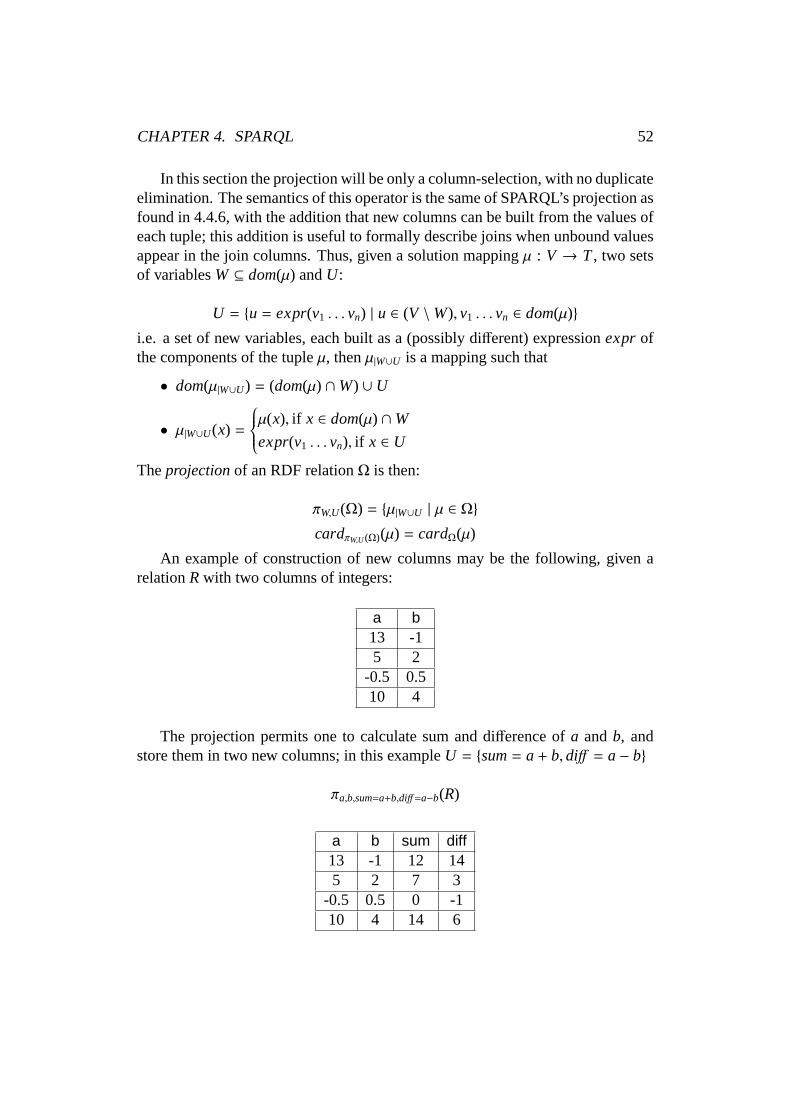
CHAPTER 4. SPARQL 52
In this section the projection will be only a column-selection, with no duplicateelimination. The semantics of this operator is the same of SPARQL’s projection asfound in 4.4.6, with the addition that new columns can be built from the values ofeach tuple; this addition is useful to formally describe joins when unbound valuesappear in the join columns. Thus, given a solution mappingµ : V → T, two setsof variablesW ⊆ dom(µ) andU:
U = u = expr(v1 . . . vn) | u ∈ (V \W), v1 . . . vn ∈ dom(µ)
i.e. a set of new variables, each built as a (possibly different) expressionexprofthe components of the tupleµ, thenµ|W∪U is a mapping such that
• dom(µ|W∪U) = (dom(µ) ∩W) ∪ U
• µ|W∪U(x) =
µ(x), if x ∈ dom(µ) ∩W
expr(v1 . . . vn), if x ∈ U
Theprojectionof an RDF relationΩ is then:
πW,U(Ω) = µ|W∪U | µ ∈ Ω
cardπW,U (Ω)(µ) = cardΩ(µ)
An example of construction of new columns may be the following, given arelationRwith two columns of integers:
a b13 -15 2
-0.5 0.510 4
The projection permits one to calculate sum and difference ofa andb, andstore them in two new columns; in this exampleU = sum= a+ b,diff = a− b
πa,b,sum=a+b,diff=a−b(R)
a b sum diff13 -1 12 145 2 7 3
-0.5 0.5 0 -110 4 14 6

CHAPTER 4. SPARQL 53
Natural join on multisets
The natural join will be used when no unbound values are present on the joinattributes. Under this assumption, the difference from the classical natural join isagain the cardinality of each tuple in the operands and in theresult, that can begreater than one in RDF relations.
The natural join in this situation behaves as normally does in relational enginesthat operate on multisets: given two RDF relationsΩL andΩR with common at-tributesv1 . . . vn, their natural join is
ΩL Z ΩR = σ ΩL.v1 = ΩR.v1...
ΩL.vn = ΩR.vn
(ΩL ×ΩR)
As usual for natural joins, the common columnsv1 . . . vn are not repeated twicein the result, one for the left and one for the right operand asin other joins, butonly once.
The cardinality of each element in the result relation conforms to the indicationof SPARQL algebra, i.e. the cardinality of a solution mappingµ in a join result is∑
µ=µL∪µRcardΩL(µL) · cardΩR(µR), that is the sum, for eachµL ∈ ΩL andµR ∈ ΩR
that may generateµ, of the product of the cardinalities of suchµL andµR.For example, given the relations
a b1 111 112 123 134 14
b c11 2111 2112 2212 2214 2415 25
their natural join is:
a b c1 11 211 11 211 11 211 11 212 12 222 12 224 14 24

CHAPTER 4. SPARQL 54
that is the correct behavior also for SPARQL.
Difference on multisets
The multiset difference is defined here as a “not in” expression: given two RDFrelationsΩL andΩR such thatvar(ΩL) = var(ΩR) i.e. with same schema, theirdifference is
ΩL \ΩR = µ ∈ ΩL | µ < ΩR
cardΩL\ΩR(µ) = cardΩL(µ)
The multiplicity of the elements does not matter: if a tuple has cardinalityequals to two inΩL and one inΩR, it will not take part in the difference.
4.5.2 Filter translation
As seen in 4.4.7, theFilter operator evaluation has to pick from a multiset ofsolutions those ones that satisfy an expression. This semantics is identical to thethe relationalselectoperator. Given a expressionexprand an RDF relationΩ:
Filter(expr,Ω) = σexpr(Ω)
EvenFilter andselectare conceptually identical, the SPARQL operators haveto deal with untyped columns; for example, a filter may selectall the triples of anRDF graph whereobject< 24. This implies also thatobjecthas to be a numericvalue.
4.5.3 BGP translation
Single pattern matching
Triple patterns (4.4.1) can be expressed as a selection of the triples of the activegraph, followed by a projection and rename. The selection condition is determinedby the fixed terms in the triple pattern. Blank nodes act exactly as variables.
For example, given the active graphG, the triple pattern
_:person foaf:name ?name
becomes
π :person← sub ject?name← ob ject
(σpredicate=foaf:name(G))
The evaluation of a triple patternt on the active graphG is a multiset of solu-tions denoted by [[t]]G.

CHAPTER 4. SPARQL 55
Triple pattern join
Given two triple patternst1 and t2 on the active graphG, and their evaluationsΩ1 = [[ t1]]G andΩ2 = [[ t2]]G,Ω1 Ztp Ω2 is a multiset defined as follows:
Ω1 Ztp Ω2 =
Ω1 ×Ω2 if var(Ω1) ∩ var(Ω2) = ∅ ∧ blank(Ω1) ∩ blank(Ω2) = ∅
Ω1 Z Ω2 if var(Ω1) ∩ var(Ω2) , ∅ ∨ blank(Ω1) ∩ blank(Ω2) , ∅
where× is the cartesian product andZ is the natural join as defined in 4.5.1.
Basic graph pattern translation
Given a BGPP = t1, t2 . . . tn and the active graphG, and denoting asΩi = [[ ti]]G
the evaluation of triple patternti, [[P]]G can be expressed as:
[[P]]G = πvar(Ω1)∪var(Ω2)...∪var(Ωn)(Ω1 Ztp Ω2 Ztp . . . Ztp Ωn)
The projection removes all columns whose name is a blank nodelabel.
4.5.4 Join translation
TheJoin definition in SPARQL is much different from the one in relational alge-bra: two mappings can be part of aJoin if there is no conflict between them, thatis when a common attribute is bound on both sides of theJoin with different val-ues. Such mappings are calledcompatible mappings. Two disjoint mappings aretherefore always compatible, and an unbound value will match with every value,even another unbound one.NULL values in relational algebra would cause the jointo fail.
Here is an example of SPARQL join between two RDF relations:
?a ?b20 121 22223 4
?b ?c1 30
314 325 33
The result is

CHAPTER 4. SPARQL 56
?a ?b ?c20 1 3020 1 3121 2 3122 1 3022 3122 4 3222 5 3323 4 3123 4 32
The SPARQLJoincan be relationally defined as a subset of the cartesian prod-uct where two mappings are compatible; given two RDF relationsΩL andΩR withcommon attributesvar(ΩL) ∩ var(ΩR) = v1 . . . vn, theCompMappingspredicatechecks if a tuple of the cross product takes part of the SPARQLJoin:
CompMappings= (ΩL.v1 = ΩR.v1 ∨ΩL.v1 = NULL ∨ΩR.v1 = NULL) ∧ . . .
∧(ΩL.vn = ΩR.vn ∨ΩL.vn = NULL ∨ΩR.vn = NULL)
TheJoinoperator can then be expressed as
Join(ΩL,ΩR) = π v1 = (ΩL.v1 , NULL ?ΩL.v1 : ΩR.v1)...
vn = (ΩL.vn , NULL ?ΩL.vn : ΩR.vn)(var(ΩL) ∪ var(ΩR)) \ v1 . . . vn
(
σCompMappings(ΩL ×ΩR))
The projection builds the columnvi from ΩL.vi andΩR.vi picking from themthe bound value, if any; it then selects all the columns that are not invar(ΩL) ∩var(ΩR). In casevar(ΩL) ∩ var(ΩR) = ∅ no selection nor projection takes placeand only the cartesian product is performed.
Another semantics for SPARQL joins may be defined when the joinattributeis only one. In this case the cartesian product can be limitedonly to those tuplesthat present an unbound value on the join attribute.
Given two RDF relationsΩL andΩR with common attributev
Join(ΩL,ΩR) = (ΩL Z ΩR)∪
π v← ΩR.v(var(ΩL) ∪ var(ΩR)) \ v
(σv=NULL(ΩL) × σv,NULL(ΩR))∪

CHAPTER 4. SPARQL 57
π v← ΩL.v(var(ΩL) ∪ var(ΩR)) \ v
(σv,NULL(ΩL) × σv=NULL(ΩR))∪
π v← ΩL.v(var(ΩL) ∪ var(ΩR)) \ v
(σv=NULL(ΩL) × σv=NULL(ΩR))
where Join is the natural join and∪ is a union that does not drop dupli-cates. The last projection can select indifferentlyΩL.v orΩR.v, since both presentNULLs on each row.
4.5.5 LeftJoin translation
Diff
The SPARQLDiff operator, given two relationsΩL andΩR and an expressionexpr, returns those mappingsµ of ΩL that either are not compatible withall themappingsµ′ ofΩR, or for which the evaluation ofexpris false for all the mappingsµ ∪ µ′.
In SPARQL these united mappings do not replicate the common attributes,while in a relational context the expressionexprhas to be evaluated against tuplesthat replicate the common attributes twice, one for the lefttuple µ and one forthe right one,µ′. If the expression is defined on one or more of these, the ex-pression has to pick the bound value, if any. Every occurrence of an attributex that participates in the join must be substituted with the ternary expression(ΩL.x , NULL ? ΩL.x : ΩR.x).
For instance, the expression:
a+ b > 4
with botha andb join attributes, has to be rewritten as
(ΩL.a , NULL ? ΩL.a : ΩR.a) + (ΩL.b , NULL ? ΩL.b : ΩR.b)
The expressionexprmodified in such manner will be denoted withexpr’.The SPARQLDiff can the be expressed with:
Diff(ΩL,ΩR,expr) = ΩL \ πvar(ΩL)
(
σCompMappings∧expr’ (ΩL ×ΩR))
The second operand of the difference builds a multiset that contains thosetuples ofΩL that are compatible at least with one tuple ofΩR, and among these,those for which at least one evaluation ofexpr is true. The result of the differencecontains therefore only tuples that are either incompatible with all the tuples ofΩR or for which the evaluation ofexpr is always false for all their combinationswith the compatible tuples ofΩR.

CHAPTER 4. SPARQL 58
LeftJoin
TheLeftJoinis expressed in the SPARQL standard as a union of aJoinand aDiff.Having already a definition of these operators in relationalalgebra, theLeftJointranslation is trivial:
LeftJoin(ΩL,ΩR,expr) =
π v1 = (ΩL.v1 , NULL ?ΩL.v1 : ΩR.v1)...
vn = (ΩL.vn , NULL ?ΩL.vn : ΩR.vn)(var(ΩL) ∪ var(ΩR)) \ v1 . . . vn
(
σCompMappings∧expr’ (ΩL ×ΩR))
∪(
ΩL \ πvar(ΩL)
(
σCompMappings∧expr’ (ΩL ×ΩR)))
4.5.6 Union translation
SPARQL union cannot be a result of any of the classical relational operators, butnonetheless there are already some implementations that define anOUTER UNION ,as described in [22]. The difference with relational union is that in this latter theschema of the tables being united must be the same. In SPARQL unions this con-dition is not needed: all the tuples of both relations take part in the result withoutduplicate elimination, and missing information is filled with unbound values. Forexample the union of the following tables
?a ?b1 212 223 234
?a ?c45 326 33
34
is

CHAPTER 4. SPARQL 59
?a ?b ?c1 212 223 23445 326 33
34
4.5.7 Graph expression translation
Graph expressions on a fixed named graph of the dataset are translated withoutany effort, since these kind of SPARQL algebra expressions just change the activegraph.
The situation in which a variable is present as graph IRI is different: in thiscase the evaluation of the graph pattern contained in the graph expression has tobe performed once for each named graph in the dataset. In 4.4.7 it has been shownthat the evaluation of a Graph pattern in this case is
[[Graph(?x,P)]] DG =
⋃
g∈name(D)
(
Join(
[[P]] DD[g] , µ?x→g
))
A relational translation is still a union of all evaluationsagainst each namedgraph; only theJoinhas to be translated.
There are two possible cases: ?x ∈ var(P), or ?x < var(P)In the first case, the join on ?x can follow the definition given in 4.5.4 for joins
on a single attribute:
[[Graph(?x,P)]] DG =
⋃
g∈name(D)
(
[[P]] DD[g] Z µ?x→g
)
∪ π ?x←?xR
var (P) \ ?x
(
σ?x=NULL
(
[[P]] DD[g]
)
× µ?x→g)
wherexR is thex column of the cross product given byµ?x→g.In the second case the only operation to perform is to extend the RDF relation
returned by [[P]] DD[g] with a column containing the graph IRIg for each tuple;
relationally, this can be done with a cartesian product:
[[Graph(?x,P)]] DG =
⋃
g∈name(D)
(
[[P]] DD[g] × µ?x→g
)

Chapter 5
RDF storage in MonetDB
5.1 Data structures
As discussed in Chapter 3, the most conventional and natural manner to store RDFtriples is a three-column relational table, with dictionary compression for IRIs andliterals.
The solution proposed in MonetDB follows this approach, butmaterializes thetriples table six times, each sorted on one of the six permutations of the columns.A single dictionary table maps integers to the RDF terms for all the views.
Figures 5.1, 5.2 and 5.3 show how some example RDF data is savedin Mon-etDB.
5.1.1 Data tables
Each of the six data tables is represented in MonetDB by threebinary tables oftype(:void, :oid) , one for each column. The virtualoid sequence identifies therow number starting from zero, while the oid column actuallystores the ids of theRDF terms.
The first column of every table is sorted by ascending id values; those triplesthat present the same value on the first column are arranged according to the idsof the second. Finally, triples with same values on the first two columns are sortedaccording to the third.
5.1.2 Dictionary table
Since the id order has to reflect the one of the RDF terms, also the dictionary hasto be sorted, so that if an id is smaller than another one then or the two termsrepresented by the ids are not comparable (e.g. because theyare different in type)or the first term is smaller than the second.
60

CHAPTER 5. RDF STORAGE IN MONETDB 61
@prefix rdf: <http://www.w3.org/1999/02/22-rdf-syntax-ns#> .
@prefix foaf: <http://xmlns.com/foaf/0.1/> .
_:f0 foaf:name "Alice" .
_:f0 foaf:mailboxes _:b0 .
_:b0 rdf:first mailto://[email protected] .
_:b0 rdf:rest _:b1 .
_:b1 rdf:first mailto://[email protected] .
_:b1 rdf:rest rdf:nil .
Figure 5.1: Example RDF data
S P O00 03 0900 05 0101 03 0801 05 0402 06 0002 07 10
P S O03 00 0903 01 0805 00 0105 01 0406 02 0007 02 10
O S P00 02 0601 00 0504 01 0508 01 0309 00 0310 02 07
S O P00 01 0500 09 0301 04 0501 08 0302 00 0602 10 07
P O S03 08 0103 09 0005 01 0005 04 0106 00 0207 10 02
O P S00 06 0201 05 0004 05 0108 03 0109 03 0010 07 02
Figure 5.2: The six materialized views
Id RDF Term00 b001 b102 f003 http://www.w3.org/1999/02/22-rdf-syntax-ns#first04 http://www.w3.org/1999/02/22-rdf-syntax-ns#nil05 http://www.w3.org/1999/02/22-rdf-syntax-ns#rest06 http://xmlns.com/foaf/0.1/mailboxes07 http://xmlns.com/foaf/0.1/name08 mailto://[email protected] mailto://[email protected] Alice
Figure 5.3: The dictionary table

CHAPTER 5. RDF STORAGE IN MONETDB 62
For the same reason terms with the same value must be mapped tothe sameinteger, even if the lexical form or the type can be different (e.g. the numbers ‘5’and ‘5.0’).
In MonetDB this table is a single BAT of type(:void, :str) , lexicographi-cally ordered on the tail. This forces one to represent everyRDF term as a stringand to make the lexicographical order be equivalent to the natural one; for numericvalues in particular, this situation required some expedient.
Order of the RDF terms
The SPARQL standard defines an ordering among the three sets that compose thesuperset of the RDF terms: blank nodes precede IRIs, which are sorted before theliterals ([44], section 9.1). The dictionary table, therefore, needs to force the orderof these terms in such manner.
The way this is achieved in Monet is to prefix every term with a single char-acter that identifies a section in the dictionary: the relative order of the sections isthus imposed by the prefixes.
The set of literals is divided into several sections; on the one hand compara-ble terms are grouped together, while on the other sections with same effectiveboolean value (see 4.4.1) are placed one next to the other. This strategy lets oneto implement the EBV function as a range check (see also figure 5.4. Finally,different sections that contain comparable terms are sorted properly (e.g. positivenumerics follow negative numerics and zero).
The following is the list of the sections in the dictionary, with their respectiveprefixes:
• Blank nodes - ‘0’
• IRIs - ‘1’
• Negative infinity - ‘2’
• Negative numerics - ‘3’
• Boolean false - ‘4’
• Numeric zero - ‘5’
• Not a Number (NaN) - ‘6’
• Empty string - ‘7’
• Empty string with language tag - ‘8’

CHAPTER 5. RDF STORAGE IN MONETDB 63
• Strings - ‘9’
• Strings with language tag - ‘A’
• Boolean true - ‘B’
• Positive Numerics - ‘C’
• Positive infinity - ‘D’
• Datetime values - ‘E’
• XML literals - ‘F’
• Literals with unsupported datatypes - ‘G’
Figure 5.4 is an example dictionary that contains at least one element in eachsection. It should be noted that sections that contain only asingle element, forexample negative and positive infinity, do not need to store anything more thanthe prefix itself: they may not even be present if the RDF document from whichdata is loaded does not contain such values.
Storing type information of literals
The dictionary does not save the XML type of numeric literalsand strings; nu-meric values can be of typexsd:integer , xsd:float , xsd:decimal and many more(see [16] for all XML datatypes), while what in the dictionary is categorized as“string” can be a simple literal (a plain literal with no language tag) or a literal oftypexsd:string .
This information cannot be lost, but cannot even be stored inthe dictionaryitself: literals with same value but different in type must be mapped to the sameidentifier. The type information is therefore stored together with the data tables,thus for each permutation of the S, P and O columns an additional BAT T of type(:void, :bte) (where:bte is the smallest type in Monet) is present.
Figure 5.5 shows a complete data table complete with its T column, but un-normalized for ease of reading.
String literals
The dictionary distinguishes four kinds of strings: empty string, empty stringswith language tag and non-empty strings, with or without language tag.
The language tag is placed in front of the lexical form, so that strings of thesame language are sorted together. This is an extension to the SPARQL standardwhich does not define an order between literals with a language tag.

CHAPTER 5. RDF STORAGE IN MONETDB 64
00
01
02
03
04
05
06
07
08
09
10
11
12
13
14
15
16
17
18
19
20
21
22
0blank0
0blank1
1http://example.com/iri1
1http://example.com/iri2
2
4
5
23
6
7
9Plain literal or string
8en
8it
B
D
F<xmlTag name="xml literal"/>
Ghttp://types.org/custom^lexicalForm
RDF termId
9Another plain literal or string
Aen@English literal
Ait@Stringa in italiano
E800b31fa01ee6280
33ff3ffffffffffff
33febffffffffffff
Cc014000000000000
Cc02b000000000000
EBV false
EBV true
EBV true
Figure 5.4: Dictionary table in detail
As said in the previous subsection, simple literals and typed strings (literalswith typexsd:string ) are grouped together and considered simply “strings”. Twostring literals with same lexical form, one typed and one not, are considered equalsand mapped to the same integer.
At the moment the current SPARQL documentation ([44], section 9.1) con-tains an inconsistency on how plain literals and typed strings should be sorted: itstates both that they are not comparable and that the typed strings follow plainliterals. A discussion on this topic with one of SPARQL’s authors can be found inthe W3C mailing list [6].
In MonetDB this problem is faced by assigning the same id to equal strings(typed or not), but at the same time giving a lower type code (in the T column) toplain literals, so that they are sorted first.

CHAPTER 5. RDF STORAGE IN MONETDB 65
S P O Tid:1 dc:value “string” plainid:2 dc:value “string” xsd:stringid:3 dc:value 5 xsd:integerid:4 dc:value 5 xsd:doubleid:5 dc:value 5 xsd:decimal
Figure 5.5: Type column for the SPO table
Numeric literals
A numeric value can be expressed in many forms, for example the literals10 ,10.0 , "10"ˆˆxsd:integer and"10.0"ˆˆxsd:float are different representations ofthe same number.
In order to assign to numeric literals with identical valuesthe same oid inthe dictionary, they are all (integers, decimal, floats etc.) converted to a double-precision representation and then converted to strings of hexadecimal characters.
The lexicographical order of these hexadecimal strings, however, is not equiv-alent to the natural one: positives would be lower than negatives, since the mostsignificant bit, the sign bit, is zero for positives; moreover negatives would besorted inversely, as shown in figure 5.6.
Value Double representation-0.50 bfe0000000000000
-0.45 bfdccccccccccccd
-0.40 bfd999999999999a
-0.35 bfd6666666666667
-0.30 bfd3333333333334
-0.25 bfd0000000000001
-0.20 bfc999999999999c
-0.15 bfc3333333333336
-0.10 bfb999999999999f
-0.05 bfa99999999999a4
0.05 3fa9999999999990
0.10 3fb9999999999995
0.15 3fc3333333333331
0.20 3fc9999999999998
0.25 3fcffffffffffffe
0.30 3fd3333333333332
0.35 3fd6666666666665
0.40 3fd9999999999998
0.45 3fdccccccccccccb
0.50 3fdffffffffffffe
Double representation Value3fa9999999999990 0.05
3fb9999999999995 0.10
3fc3333333333331 0.15
3fc9999999999998 0.20
3fcffffffffffffe 0.25
3fd3333333333332 0.30
3fd6666666666665 0.35
3fd9999999999998 0.40
3fdccccccccccccb 0.45
3fdffffffffffffe 0.50
bfa99999999999a4 -0.05
bfb999999999999f -0.10
bfc3333333333336 -0.15
bfc999999999999c -0.20
bfd0000000000001 -0.25
bfd3333333333334 -0.30
bfd6666666666667 -0.35
bfd999999999999a -0.40
bfdccccccccccccd -0.45
bfe0000000000000 -0.50
Figure 5.6: Numeric values and their double representation, sorted on value onthe left and on the representation on the right
A simple solution consists in XORing the 64 bits of the double representation.Two different bit masks are needed, one for positive and one for negative numbers.

CHAPTER 5. RDF STORAGE IN MONETDB 66
The first has just to invert the first bit (i.e.8000000000000000 in hexadecimaldigits), while the second and to revert every bit (i.e.ffffffffffffffff ). Theresult is shown in figure 5.7.
Value Representation-0.50 401fffffffffffff
-0.45 4023333333333332
-0.40 4026666666666665
-0.35 4029999999999998
-0.30 402ccccccccccccb
-0.25 402ffffffffffffe
-0.20 4036666666666663
-0.15 403cccccccccccc9
-0.10 4046666666666660
-0.05 405666666666665b
0.05 bfa9999999999990
0.10 bfb9999999999995
0.15 bfc3333333333331
0.20 bfc9999999999998
0.25 bfcffffffffffffe
0.30 bfd3333333333332
0.35 bfd6666666666665
0.40 bfd9999999999998
0.45 bfdccccccccccccb
0.50 bfdffffffffffffe
Figure 5.7: Representation order reflects value order
xsd:dateTime literals
Literals with XML type xsd:dateTime are stored as a concatenation of Monet’stimestamp (a 64-bit binary format), converted to a string ofhexadecimal charac-ters, with a character string that stores the fractions of a second. The concatenationis needed because the fractions of a second in Monet have millisecond precision,while they may contain an unspecified number of digits in XML’s type system.
If a timezone information is present, the timestamp is converted and storedin UTC, and when returned by a query it has to be converted back to the client’stimezone. If this information is not present, the timestampis saved and returned“as is”, without any conversion. In order to distinguish between datetimes withand without timezone, the RDF module defines two internal subtypes, whose codeis stored in the T column of the data table.
Also in this case, two datetime literals with same value are mapped to thesame numeric identifier. Two literals with same date and timevalues, one withouttimezone information and the other in UTC are considered equals as well.
So as the double-precision representation of numbers, alsoMonet’s times-tamps need to be XORed with a bitmask to let the lexical order beequivalent tothe natural one. The mask in this case has just to reverse the first bit.

CHAPTER 5. RDF STORAGE IN MONETDB 67
Figure 5.8 shows some datetime literals and their representations in the dictio-nary table, without prefix. Literals with same representation are obviously mappedto the same identifier.
XML dateTime Representation2007-08-07T21:15:00 800b304c048f4c20
2008-07-07T21:15:00 800b319b048f4c20
2008-08-06T21:15:00 800b31b9048f4c20
2008-08-07T20:15:00 800b31ba04585da0
2008-08-07T21:14:00 800b31ba048e61c0
2008-08-07T21:14:59 800b31ba048f4838
2008-08-07T21:14:59.999 800b31ba048f4838999
2008-08-07T21:15:00 800b31ba048f4c20
2008-08-07T21:15:00+00:00 800b31ba048f4c20
2008-08-07T22:15:00+01:00 800b31ba048f4c20
2008-08-07T20:15:00-01:00 800b31ba048f4c20
2008-08-07T21:15:00.0123 800b31ba048f4c200123
2008-08-07T21:15:00.123 800b31ba048f4c20123
2008-08-07T21:15:00.987+00:00 800b31ba048f4c20987
2008-08-07T21:15:00.9876+00:00 800b31ba048f4c209876
Figure 5.8: Representation order reflects value order
Unsupported datatypes andrdf:XMLLiteral
Numeric, boolean, string and datetime literals have a special treatment since theyare required by SPARQL’s standard operators, but other kind of literals may ap-pear in RDF documents as well.
In general, they are stored in section ‘G’, with the datatypeIRI as a prefix ofthe lexical form; in this manner literals of the same type aregrouped together andsorted on the lexical form.
Literals of typerdf:XMLLiteral , that are XML strings embedded in an RD-F/XML document, are stored separately in section ‘F’; hence they do not need toinclude the datatype IRI together with the lexical form.
5.2 Importing algorithm
The RDF document importing is performed in two phases; in the first one thedocument is parsed and a first dictionary and data table (withcolumns S, P, O andT) are filled incrementally. In the second phase the dictionary is sorted and the sixpermutations of the data tables are created.

CHAPTER 5. RDF STORAGE IN MONETDB 68
5.2.1 First phase
MonetDB uses the Raptor Library [12] to parse RDF. This libraryinvokes a call-back function for each triple of the document, that can be expressed in almostevery RDF serialization language.
Each time the triples handler function is called, MonetDB inserts a mappingin the dictionary for every term in the triple not previouslyencountered, and addsa row in the data table with the ids of terms and the one-byte code of the object’stype.
Figure 5.10 shows the situation after the first phase of the importing of theRDF data in figure 5.1, which is copied to figure 5.9 for ease of reading (T columnis omitted).
@prefix rdf: <http://www.w3.org/1999/02/22-rdf-syntax-ns#> .
@prefix foaf: <http://xmlns.com/foaf/0.1/> .
_:f0 foaf:name "Alice" .
_:f0 foaf:mailboxes _:b0 .
_:b0 rdf:first mailto://[email protected] .
_:b0 rdf:rest _:b1 .
_:b1 rdf:first mailto://[email protected] .
_:b1 rdf:rest rdf:nil .
Figure 5.9: Example RDF data
Id RDF Term00 0f001 1http://xmlns.com/foaf/0.1/name02 9Alice03 1http://xmlns.com/foaf/0.1/mailboxes04 0b005 1http://www.w3.org/1999/02/22-rdf-syntax-ns#first06 1mailto://[email protected] 1http://www.w3.org/1999/02/22-rdf-syntax-ns#rest08 0b109 1mailto://[email protected] 1http://www.w3.org/1999/02/22-rdf-syntax-ns#nil
S P O00 01 0200 03 0404 05 0604 07 0808 05 0908 07 10
Figure 5.10: Dictionary and data table after the first phase of importing

CHAPTER 5. RDF STORAGE IN MONETDB 69
5.2.2 Second phase – sorting
Sorting the dictionary
The first step of the second phase sorts the dictionary on the tail. As said above,this is a simple lexicographical sort, for which MonetDB is highly optimized.Since the head of the BAT is not a sequence anymore, it cannot be of type:voidbut it is rather materialized and of type:oid , as shown in figure 5.11.
Id RDF Term04 0b008 0b100 0f005 1http://www.w3.org/1999/02/22-rdf-syntax-ns#first10 1http://www.w3.org/1999/02/22-rdf-syntax-ns#nil07 1http://www.w3.org/1999/02/22-rdf-syntax-ns#rest03 1http://xmlns.com/foaf/0.1/mailboxes01 1http://xmlns.com/foaf/0.1/name09 1mailto://[email protected] 1mailto://[email protected] 9Alice
Figure 5.11: Dictionary just after sorting
Id translation
The final dictionary in figure 5.12 has the same tail of the BAT in figure 5.11, butwith a :void sequence on the head; a mapping of the ids created during the RDFdocument parsing and the final ones is therefore needed. Thismapping is createdas avoid view (see 2.4) of the head of the dictionary in figure 5.11, as shown infigure 5.13.
This BAT is joined with the S, P and O BATs, creating a new triples table withthe final identifiers, shown in figure 5.14.
Sorting the triples table
The last step of the process creates the six copies of the triples table. The algorithmsorts one of three columns, then refines the order of the othertwo columns twice,one for each permutation of the these latters. For example, if it sorts first the Scolumn, then it refines the order on P and subsequently on O , creating a triplestable ordered on SPO; then it refines the order on O and P, creating the SOP table.
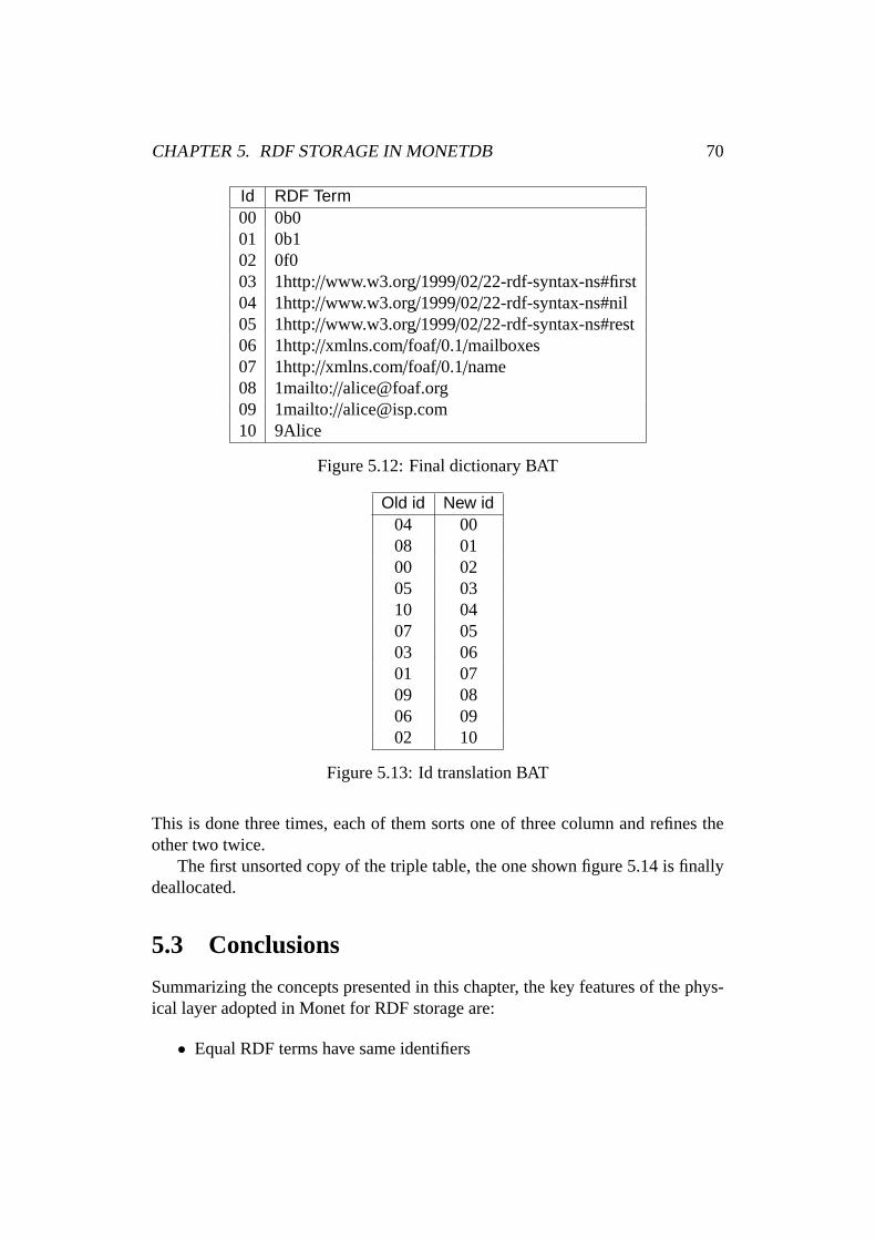
CHAPTER 5. RDF STORAGE IN MONETDB 70
Id RDF Term00 0b001 0b102 0f003 1http://www.w3.org/1999/02/22-rdf-syntax-ns#first04 1http://www.w3.org/1999/02/22-rdf-syntax-ns#nil05 1http://www.w3.org/1999/02/22-rdf-syntax-ns#rest06 1http://xmlns.com/foaf/0.1/mailboxes07 1http://xmlns.com/foaf/0.1/name08 1mailto://[email protected] 1mailto://[email protected] 9Alice
Figure 5.12: Final dictionary BAT
Old id New id04 0008 0100 0205 0310 0407 0503 0601 0709 0806 0902 10
Figure 5.13: Id translation BAT
This is done three times, each of them sorts one of three column and refines theother two twice.
The first unsorted copy of the triple table, the one shown figure 5.14 is finallydeallocated.
5.3 Conclusions
Summarizing the concepts presented in this chapter, the keyfeatures of the phys-ical layer adopted in Monet for RDF storage are:
• Equal RDF terms have same identifiers

CHAPTER 5. RDF STORAGE IN MONETDB 71
S P O02 07 1002 06 0000 03 0900 05 0101 03 0801 05 04
Figure 5.14: Triples table with final ids
• The order of two comparable RDF terms is the same of their identifiers
• The data is sorted in all possible ways
• Data with same EBV is grouped together
These characteristics permit to obtain several advantages, in terms of searchesand joins.
Fast searches and EBV predicate evaluations
One of the most important advantages is that every string search in the dictionaryand every id search in the six data tables are performed on sorted data, allowingto implement range selects asslice views, as discussed in section 2.4.
An id lookup in the dictionary can be performed by position, i.e. the fastestway possible; every join between the data tables and the dictionary is therefore apositional join.
The search of values in the data tables, moreover, can be performed in theidentifier space, thus not requiring a join with the dictionary; a SPARQL triplepattern like?s foaf:name "Alice" , for example, can be implemented as a searchin the POS or OPS table of those triples that have the id offoaf:name in P and theid of "Alice" in O. The join with the dictionary is needed only at the end of queryexecution, before returning the result.
Fast joins
As with searches, value-based joins can be performed in the id space, since identi-fier equality assures equality of the RDF terms, and conversely identifier inequal-ity assures inequality of the terms. As in any relational engine, MonetDB joinsids much faster than strings.
One of the greatest issues of SPARQL is that requires many selfequi-joins ofthe triples table, that can be an important bottleneck in many relational engines, as

CHAPTER 5. RDF STORAGE IN MONETDB 72
discussed in [9], [21]. The approach adopted in MonetDB permits one to performmerge-joins in many situations, or to have very often at least one of the operandssorted on the join column; also a nested loop would perform much faster in thiscase if this table is chosen as inner table.
The following two example queries permit one to better guessthe above ad-vantages; all SPARQL queries are translated to relational algebra, and their exe-cution explained. Theselectoperations make use of theId(RDF-Term t)function,that returns the identifier of the given RDF term, or a special value to suggest thatthe term is not present in the dictionary; in this case theselectreturns an emptyset. The final join with the dictionary to convert back ids is omitted.
This simple query can found in the current SPARQL specification:
PREFIX foaf: <http://xmlns.com/foaf/0.1/>
SELECT ?name ?mbox
WHERE
?x foaf:name ?name .
?x foaf:mbox ?mbox
In algebra it can be expressed as:
π ?name?mbox
(
π ?x← s?name← o
(
σp = Id (foaf : name) (PSO))
Z π ?x← s?mbox← o
(
σp = Id (foaf : mbox) (PSO))
)
The selections on P are very fast since the data in PSO is sorted on that columnand are thus implemented as slice views. Choosing the PSO table, moreover,assures that the S column is sorted for a given value of P, thatis id of foaf:nameon the left table of the join and the id offoaf:mbox on the right. Since the join ison S, a merge-join (on the ids) can be performed.
The following query looks for the titles of the resources referenced by thosesubjects ?s, whose title is “RDF”:
PREFIX dc: <http://purl.org/dc/elements/1.1/> .
PREFIX rdfs: <http://www.w3.org/2000/01/rdf-schema#> .
SELECT ?seeAlso
WHERE
?s dc:title "RDF".
?s rdfs:seeAlso :?x .
?x dc:title ?seeAlso
It can be translated as
(
σ o = Id (“RDF” )p = Id (dc : title)
(OPS) Z π?x← o
(
σp = Id (rdfs : seeAlso) (PSO))
)
Z π?x← s
(
σp = Id (dc : title) (POS))
Again, all theselectoperations are on sorted data, and the inmost join is per-formed on two sorted columns. Even if the left operand of the last join is not

CHAPTER 5. RDF STORAGE IN MONETDB 73
sorted on ?x, nevertheless the right one is, thus it can be used efficiently as theinner table of a nested loop join; if the left operand is not enormous, moreover,Monet can still decide to sort it. Another benefit of MonetDB’sapproach in thisexample is that self joins are avoided, since the three triple patterns operate onthree distinct tables.
Although these examples are not barely comprehensive and more exhaustiveexperiments have to be carried out, the possible benefits of the RDF storage tech-nique adopted in MonetDB, and especially of the exploitationof the sorted anddense properties, should be clear.
Drawbacks
The advantages of having the data tables replicated six times are followed by theirdisk occupation. For these reason it is already planned thatMonetDB/SPARQLwill adopt lightweight compression of the data, following its application in Monet-DB/X100 [52, 54], and for which an extensive literature is present in the databasefield [23, 28, 32]).
The dense identifier set makes updates impossible to be merged seamlessly inthe proposed design, but they can be rather kept in separate aDelta structure thatkeeps track of all the modifications. If theDeltagrows until the performance getsnoticeably worse, it will be possible to merge it, creating anew dictionary and anew set of data tables.
The particular way the data is stored in the dictionary requires that even themost trivial functions have to be reimplemented in order to deal with this repre-sentation: a simple SPARQLFILTER like ?o < 50 , for example, has to be RDF-specific: the implementation has to transform 50 in its hexadecimal string rep-resentation, find the id of the nearest value to it in the dictionary,max , and thesmallest numeric value,min , and finally express the filter as a range select of idsgreater thanmin and smaller thanmax , or equal to the id of zero.
Since different RDF graphs are stored in different sets of tables, a query thatinvolves multiple graphs cannot benefit from all the advantages described above,since the assumptions on the order and equality of the identifiers are lost. Evenif graph-specific operations can be optimized in this sense,joining data from dif-ferent graphs cannot be done in the id space. For this reason it will be possiblefor a database administrator to merge two or more graphs if a set of queries isfrequently executed against those graphs.

Appendix A
Materialized view choice
This appendix shows which are the best materialized views that the MonetDB/-SPARQL optimizer can choose when it has to evaluate a Basic Graph Pattern. Thetarget is to perform selections and joins on sorted columns.
The first two sections of the appendix examine all BGPs of one and two triplepatterns respectively, dividing them according to the number of fixed terms inthem. The considered kind of joins aresubject-subject, subject-objectandobject-object.
The last section shows how this information can be used to plan the executionof more complex queries.
A.1 Single triple pattern BGPs
In this simple situation the optimizer would chose the view on the basis of theORDER BY clause or, if other group graph patterns are present, on the basis of thekind of join that have to performed higher in the execution plan.
A.1.1 3 variables
View Result orderSPO (?s, ?p, ?o)SOP (?s, ?o, ?p)PSO (?p, ?s, ?o)POS (?p, ?o, ?s)OSP (?o, ?s, ?p)OPS (?o, ?p, ?s)
74

APPENDIX A. MATERIALIZED VIEW CHOICE 75
A.1.2 2 variables
• f ?p ?o
View Result orderSPO (?p, ?o)SOP (?o, ?p)
• ?s f ?o
View Result orderPSO (?s, ?o)POS (?o, ?s)
• ?s ?p f
View Result orderOSP (?s, ?p)OPS (?p, ?s)
A.1.3 1 variable
The choice here depend on the selectivity of thef0 and f1 constraints. In the thirdpattern for instance, the constraint on O is usually much more selective than theone on P, making therefore OPS a better choice.
• f0 f1 ?o
View Result orderSPO or PSO (?o)
• f0 ?p f1
View Result orderSOP or OSP (?p)
• ?s f0 f1
View Result orderPOS or OPS (?s)

APPENDIX A. MATERIALIZED VIEW CHOICE 76
A.2 BGPs of two triple patterns
In many cases in this section the result can be ordered in two different ways. Thisdepends on the merge join behaviour when the sameoid is encountered multipletimes in the join column ?x on both sides, since in these ranges the algorithmperforms a nested-loop: for eachoid of the outer table, it loops on the inner oneuntil a differentoid is found. In the result, the outer table has its columns sortedbefore those of the inner one.
The optimizer can choose which should be the outer table on the basis itsneeds.
A.2.1 No constraints
BGP View 1 View 2 Result order
?x ?p1 ?o1 .?x ?p2 ?o2
SPO SPO(?x, ?p1, ?o1, ?p2, ?o2)
or(?x, ?p2, ?o2, ?p1, ?o1)
?x ?p1 ?o1 .?x ?p2 ?o2
SPO SOP(?x, ?p1, ?o1, ?o2, ?p2)
or(?x, ?o2, ?p2, ?p1, ?o1)
?x ?p1 ?o1 .?x ?p2 ?o2
SOP SPO(?x, ?o1, ?p1, ?p2, ?o2)
or(?x, ?p2, ?o2, ?o1, ?p1)
?x ?p1 ?o1 .?x ?p2 ?o2
SOP SOP(?x, ?o1, ?p1, ?o2, ?p2)
or(?x, ?o2, ?p2, ?o1, ?p1)
?x ?p1 ?o1 .?s2 ?p2 ?x
SPO OPS(?x, ?p1, ?o1, ?p2, ?s2)
or(?x, ?p2, ?s2, ?p1, ?o1)
?x ?p1 ?o1 .?s2 ?p2 ?x
SPO OSP(?x, ?p1, ?o1, ?s2, ?p2)
or(?x, ?s2, ?p2, ?p1, ?o1)
?x ?p1 ?o1 .?s2 ?p2 ?x
SOP OPS(?x, ?o1, ?p1, ?p2, ?s2)
or(?x, ?p2, ?s2, ?o1, ?p1)
?x ?p1 ?o1 .?s2 ?p2 ?x
SOP OSP(?x, ?o1, ?p1, ?s2, ?p2)
or(?x, ?s2, ?p2, ?o1, ?p1)

APPENDIX A. MATERIALIZED VIEW CHOICE 77
BGP View 1 View 2 Result order
?s1 ?p1 ?x .?x ?p2 ?o2
OPS SPO(?x, ?p1, ?s1, ?p2, ?o2)
or(?x, ?p2, ?o2, ?p1, ?s1)
?s1 ?p1 ?x .?x ?p2 ?o2
OPS SOP(?x, ?p1, ?s1, ?o2, ?p2)
or(?x, ?o2, ?p2, ?p1, ?s1)
?s1 ?p1 ?x .?x ?p2 ?o2
OSP SPO(?x, ?s1, ?p1, ?p2, ?o2)
or(?x, ?p2, ?o2, ?s1, ?p1)
?s1 ?p1 ?x .?x ?p2 ?o2
OSP SOP(?x, ?s1, ?p1, ?o2, ?p2)
or(?x, ?o2, ?p2, ?s1, ?p1)
?s1 ?p1 ?x .?s2 ?p2 ?x
OPS OPS(?x, ?p1, ?s1, ?p2, ?s2)
or(?x, ?p2, ?s2, ?p1, ?s1)
?s1 ?p1 ?x .?s2 ?p2 ?x
OPS OSP(?x, ?p1, ?s1, ?s2, ?p2)
or(?x, ?s2, ?p2, ?p1, ?s1)
?s1 ?p1 ?x .?s2 ?p2 ?x
OSP OPS(?x, ?s1, ?p1, ?p2, ?s2)
or(?x, ?p2, ?s2, ?s1, ?p1)
?s1 ?p1 ?x .?s2 ?p2 ?x
OSP OSP(?x, ?s1, ?p1, ?s2, ?p2)
or(?x, ?s2, ?p2, ?s1, ?p1)
A.2.2 1 constraint
• Constraint on subject f ?p1 ?o1 .
?s2 ?p2 ?o2
BGP View 1 View 2 Result order
f ?p1 ?x .?x ?p2 ?o2
SOP SPO(?x, ?p1, ?p2, ?o2)
or(?x, ?p2, ?o2, ?p1)
f ?p1 ?x .?x ?p2 ?o2
SOP SOP(?x, ?p1, ?o2, ?p2)
or(?x, ?o2, ?p2, ?p1)

APPENDIX A. MATERIALIZED VIEW CHOICE 78
BGP View 1 View 2 Result order
f ?p1 ?x .?s2 ?p2 ?x
SOP OPS(?x, ?p1, ?p2, ?s2)
or(?x, ?p2, ?s2, ?p1)
f ?p1 ?x .?s2 ?p2 ?x
SOP OSP(?x, ?p1, ?s2, ?p2)
or(?x, ?s2, ?p2, ?p1)
• Constraint on property ?s1 f ?o1 .
?s2 ?p2 ?o2
BGP View 1 View 2 Result order
?x f ?o1 .?x ?p2 ?o2
PSO SPO(?x, ?o1, ?p2, ?o2)
or(?x, ?p2, ?o2, ?o1)
?x f ?o1 .?x ?p2 ?o2
PSO SOP(?x, ?o1, ?o2, ?p2)
or(?x, ?o2, ?p2, ?o1)
?x f ?o1 .?s2 ?p2 ?x
PSO OSP(?x, ?o1, ?s2, ?p2)
or(?x, ?s2, ?p2, ?o1)
?x f ?o1 .?s2 ?p2 ?x
PSO OPS(?x, ?o1, ?p2, ?s2)
or(?x, ?p2, ?s2, ?o1)
?s1 f ?x .?x ?p2 ?o2
POS SPO(?x, ?s1, ?p2, ?o2)
or(?x, ?p2, ?o2, ?s1)
?s1 f ?x .?x ?p2 ?o2
POS SOP(?x, ?s1, ?o2, ?p2)
or(?x, ?o2, ?p2, ?s1)
?s1 f ?x .?s2 ?p2 ?x
POS OSP(?x, ?s1, ?s2, ?p2)
or(?x, ?s2, ?p2, ?s1)
?s1 f ?x .?s2 ?p2 ?x
POS OPS(?x, ?s1, ?p2, ?s2)
or(?x, ?p2, ?s2, ?s1)
• Constraint on object ?s1 ?p1 f .
?s2 ?p2 ?o2

APPENDIX A. MATERIALIZED VIEW CHOICE 79
BGP View 1 View 2 Result order
?x ?p1 f .?x ?p2 ?o2
OSP SPO(?x, ?p1, ?p2, ?o2)
or(?x, ?p2, ?o2, ?p1)
?x ?p1 f .?x ?p2 ?o2
OSP SOP(?x, ?p1, ?o2, ?p2)
or(?x, ?o2, ?p2, ?p1)
?x ?p1 f .?s2 ?p2 ?x
OSP OSP(?x, ?p1, ?s2, ?p2)
or(?x, ?s2, ?p2, ?p1)
?x ?p1 f .?s2 ?p2 ?x
OSP OPS(?x, ?p1, ?p2, ?s2)
or(?x, ?p2, ?s2, ?p1)
A.2.3 2 constraints
• fa fb ?o1 .
?s2 ?p2 ?o2
BGP View 1 View 2 Result order fa fb ?x .
?x ?p2 ?o2 SPO or PSO SPO (?x, ?p2, ?o2)
fa fb ?x .?x ?p2 ?o2
SPO or PSO SOP (?x, ?o2, ?p2)
fa fb ?x .?s1 ?p2 ?x
SPO or PSO OSP (?x, ?s2, ?p2)
fa fb ?x .?s1 ?p2 ?x
SPO or PSO OPS (?x, ?p2, ?s2)
• fa ?p1 ?o1 .
fb ?p2 ?o2
BGP View 1 View 2 Result order
fa ?p1 ?x .fb ?p2 ?x
SOP SOP(?x, ?p1, ?p2)
or(?x, ?p2, ?p1)
• fa ?p1 ?o1 .
?s2 fb ?o2

APPENDIX A. MATERIALIZED VIEW CHOICE 80
BGP View 1 View 2 Result order
fa ?p1 ?x .?x fb ?o2
SOP PSO(?x, ?p1, ?o2)
or(?x, ?o2, ?p1)
fa ?p1 ?x .?s2 fb ?x
SOP POS(?x, ?p1, ?s2)
or(?x, ?s2, ?p1)
• fa ?p1 ?o1 .
?s2 ?p2 fb
BGP View 1 View 2 Result order
fa ?p1 ?x .?x ?p2 fb
SOP OSP(?x, ?p1, ?p2)
or(?x, ?p2, ?p1)
• ?s1 fa fb .
?s2 ?p2 ?o2
BGP View 1 View 2 Result order ?x fa fb .
?x ?p2 ?o2 POS or OPS SPO (?x, ?p2, ?o2)
?x fa fb .?x ?p2 ?o2
POS or OPS SOP (?x, ?o2, ?p2)
?x fa fb .?s2 ?p2 ?x
POS or OPS OSP (?x, ?s2, ?p2)
?x fa fb .?s2 ?p2 ?x
POS or OPS OPS (?x, ?p2, ?s2)
• ?s1 fa ?o1 .
?s2 fb ?o2

APPENDIX A. MATERIALIZED VIEW CHOICE 81
BGP View 1 View 2 Result order
?x fa ?o1 .?x fb ?o2
PSO PSO(?x, ?o1, ?o2)
or(?x, ?o2, ?o1)
?x fa ?o1 .?s2 fb ?x
PSO POS(?x, ?o1, ?s2)
or(?x, ?s2, ?o1)
?s1 fa ?x .?x fb ?o2
POS PSO(?x, ?s1, ?o2)
or(?x, ?o2, ?s1)
?s1 fa ?x .?s2 fb ?x
POS POS(?x, ?s1, ?s2)
or(?x, ?s2, ?s1)
• ?s1 fa ?o1 .
?s2 ?p2 fb
BGP View 1 View 2 Result order
?x fa ?o1 .?x ?p2 fb
PSO OSP(?x, ?o1, ?p2)
or(?x, ?p2, ?o1)
?s1 fa ?x .?x ?p2 fb
POS OSP(?x, ?s1, ?p2)
or(?x, ?p2, ?s1)
• ?s1 ?p1 fa .
?s2 ?p2 fb
BGP View 1 View 2 Result order
?x ?p1 fa .?x ?p2 fb
OSP OSP(?x, ?p1, ?p2)
or(?x, ?p2, ?p1)
A.2.4 3 constraints
• fa fb ?o1 .
fc ?p2 ?o2
BGP View 1 View 2 Result order fa fb ?x .
fc ?p2 ?x SPO or PSO SOP (?x, ?p2)

APPENDIX A. MATERIALIZED VIEW CHOICE 82
• fa fb ?o1 .
?s2 fc ?o2
BGP View 1 View 2 Result order fa fb ?x .
?x fc ?o2 SPO or PSO PSO (?x, ?o2)
fa fb ?x .?s2 fc ?x
SPO or PSO POS (?x, ?s2)
• fa fb ?o1 .
?s2 ?p2 fc
BGP View 1 View 2 Result order fa fb ?x .
?x ?p2 fc SPO or PSO OSP (?x, ?p2)
• fa ?p1 ?o1 .
?s2 fb fc
BGP View 1 View 2 Result order fa ?p1 ?x .
?x fb fc SOP POS or OPS (?x, ?p1)
• ?s1 fa fb .
?s2 fc ?o2
BGP View 1 View 2 Result order ?x fa fb .
?x fc ?o2 POS or OPS PSO (?x, ?o2)
?x fa fb .?s2 fc ?x
POS or OPS POS (?x, ?s2)
• ?s1 fa fb .
?s2 ?p2 fc
BGP View 1 View 2 Result order ?x fa fb .
?x ?p2 fc POS or OPS OSP (?x, ?p2)
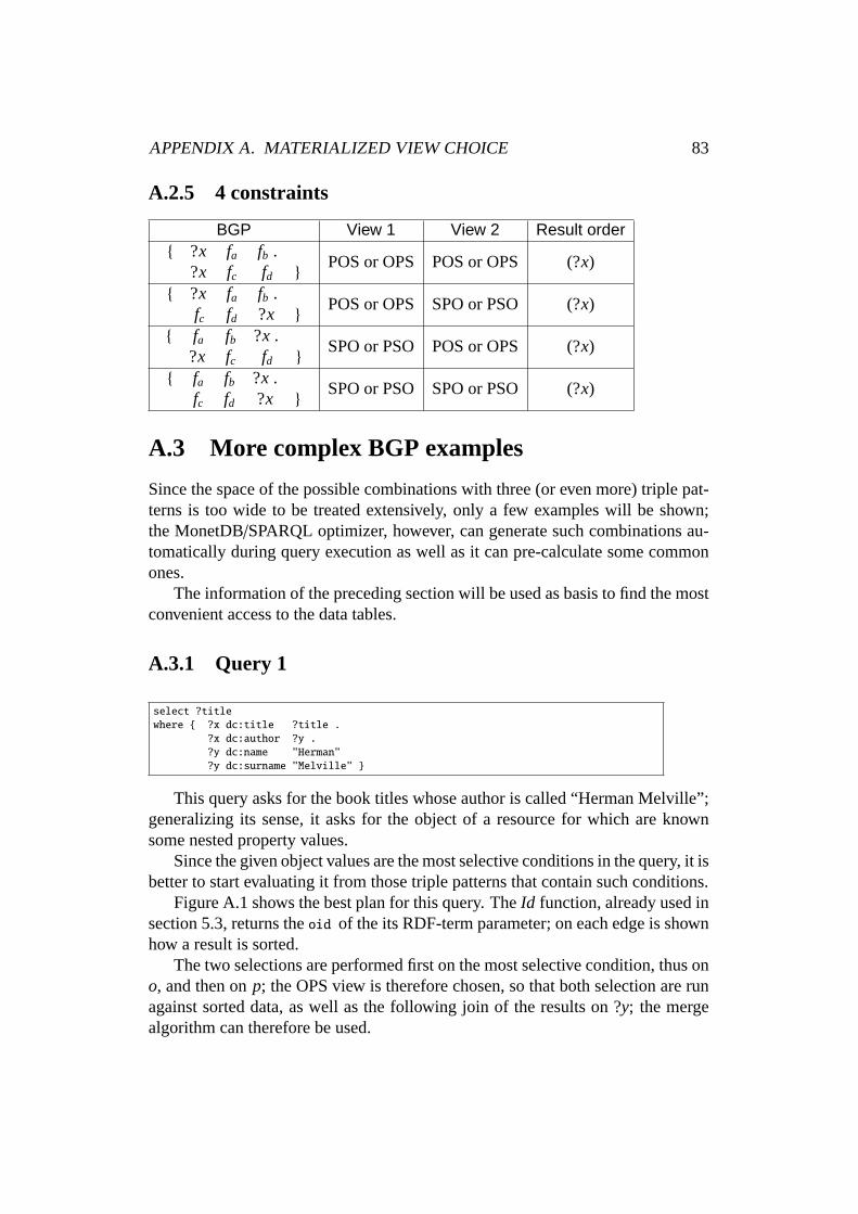
APPENDIX A. MATERIALIZED VIEW CHOICE 83
A.2.5 4 constraints
BGP View 1 View 2 Result order ?x fa fb .
?x fc fd POS or OPS POS or OPS (?x)
?x fa fb .fc fd ?x
POS or OPS SPO or PSO (?x)
fa fb ?x .?x fc fd
SPO or PSO POS or OPS (?x)
fa fb ?x .fc fd ?x
SPO or PSO SPO or PSO (?x)
A.3 More complex BGP examples
Since the space of the possible combinations with three (or even more) triple pat-terns is too wide to be treated extensively, only a few examples will be shown;the MonetDB/SPARQL optimizer, however, can generate such combinations au-tomatically during query execution as well as it can pre-calculate some commonones.
The information of the preceding section will be used as basis to find the mostconvenient access to the data tables.
A.3.1 Query 1
select ?title
where ?x dc:title ?title .
?x dc:author ?y .
?y dc:name "Herman"
?y dc:surname "Melville"
This query asks for the book titles whose author is called “Herman Melville”;generalizing its sense, it asks for the object of a resource for which are knownsome nested property values.
Since the given object values are the most selective conditions in the query, it isbetter to start evaluating it from those triple patterns that contain such conditions.
Figure A.1 shows the best plan for this query. TheId function, already used insection 5.3, returns theoid of the its RDF-term parameter; on each edge is shownhow a result is sorted.
The two selections are performed first on the most selective condition, thus ono, and then onp; the OPS view is therefore chosen, so that both selection arerunagainst sorted data, as well as the following join of the results on ?y; the mergealgorithm can therefore be used.

APPENDIX A. MATERIALIZED VIEW CHOICE 84
(?y)
(?y, ?x, ?title)
(?y)
(?y) (?y, ?x)
(?y, ?x)
OPS
POS
(?x, ?title)
PSO
OPS
ρ?y←s(σo=Id(“Herman”)∧p=Id(dc:name))
ρ?y←s(σo=Id(“Melville”) ∧p=Id(dc:surname))
ρ ?y← o?x← s
(σp=Id(dc:author))
ρ ?x← s?title← o
(σp=Id(dc:title))
Z
Z
Z
Figure A.1:
As any selection on the data table, also the one POS is performed on ordereddata. The result is sorted on ?y making another merge join possible, but sincethe cardinality of the left operand is expected to be very low, instead of scanningthe full table as a merge join would normally do, it would be better to perform abinary search on the right operand for each value in the left one.
The same happens in the last join, where the left operand is again small andthe search in the right operand is performed on the sorted column ?x.
A.3.2 Query 2
select ?title ?name ?mbox
where ?person foaf:publication ?doc .
?doc dc:title ?title .
?person foaf:mbox ?mbox .
?person foaf:name ?name
This query lists all the names and emails of those people who published oneor more documents, along with the titles of these.
This query can have huge intermediate results if the datasetis large: the joinorder chosen in figure A.2 keeps them as small as possible, as well as choosingthe views in order to join sorted data.
If the first join combined the result of the selection onp=foaf:publication andp=foaf:mbox which are both multi-valued properties, the intermediate result wouldbe much bigger than in the case shown in figure, sincefoaf:name is a single-valuedproperty.
Also in this query the first two joins can be merge-joins, while the last hasonly its right operand ordered.

APPENDIX A. MATERIALIZED VIEW CHOICE 85
(?person, ?doc, ?name) (?person, ?mbox)
(?person, ?doc, ?name, ?mbox)
(?person, ?doc, ?name, ?mbox, ?title)
PSO
(?person, ?name)
PSO
PSO
(?person, ?doc)
(?doc, ?title)
PSO
ρ ?person← s?doc← o
(σp=Id(foaf:publication))
ρ ?person← s?name← o
(σp=Id(foaf:name))
ρ ?person← s?mbox← o
(σp=Id(foaf:mbox)
ρ ?doc← s?title← o
(σp=Id(dc:title)Z
Z
Z
Figure A.2:
A.3.3 Query 3
prefix m: <http://motorbikeontology.org/terms/>
select ?name ?price
where ?bike m:modelname ?name .
?bike m:engine ?engine .
?engine m:cylinders 3 .
?bike dc:price ?price
FILTER(?price < 7000)
The query searches for those motorbikes that have a three-cylinder engine anda price lower than 7000 Euros.
Two different plans are shown: the first (fig. A.3) selects the bikes with therequested price and joins the result first with the bikes withthree cylinders andthen retrieves their names; the second (fig. A.4) pulls the selection on price up,looking first for the bikes with the requested engine, then retrieving their namesand prices and finally selecting the right price from the result.
The second approach has the advantage to perform only merge joins, exceptthe first one (the leftmost in figure A.4), but the final select on the price has to scanthe full result. The first can perform the selection on price with an almost free ofcost slice view 2.4, but it cannot perform merge joins; it cananyway count on thefact that at least one operand has always the join column sorted.
The selections on price take also the POSNUM MIN ID argument, that rep-resents theoid of the smallest positive numeric in MonetDB’s dictionary.

APPENDIX A. MATERIALIZED VIEW CHOICE 86
OPS
PSO OPS
(?bike, ?engine)(?price, ?bike)
(?engine)(?bike, ?engine)
(?price, ?bike, ?engine)
(?price, ?bike, ?engine, ?name)
(?bike, ?name)
PSO
σp=Id(m:engine) σo=Id(3)∧p=Id(m:cylinders)
σPOSNUM MIN ID<o<Id(7000)∧p=Id(dc:price)
σp=Id(dc:modelname)
Z
Z
Z
Figure A.3:
PSO OPS
(?engine)(?bike, ?engine)
(?bike, ?engine) (?bike, ?name)
PSO
(?bike, ?name, ?engine)
PSO
(?bike, ?price)
(?bike, ?price, ?name, ?engine)
σp=Id(m:engine) σo=Id(3)∧p=Id(m:cylinders)
σp=Id(dc:price)
σp=Id(dc:modelname)
σPOSNUM MIN ID<?price<Id(7000)
Z
Z
Z
Figure A.4:

Bibliography
[1] Centrum voor Wiskunde en Informatica .http://www.cwi.nl/.
[2] MonetDB - Query Processing at Light Speed.http://monetdb.cwi.nl/.
[3] OpenLink Virtuoso - RDF Database and SPARQL.http://docs.openlinksw.com/virtuoso/rdfdatarepresentation.html.
[4] RDF Issue Tracking. http://www.w3.org/2000/03/rdf-tracking/#rdfms-literalsubjects.
[5] Resource Description Framework (RDF)/ W3C Semantic Web Activity.http://www.w3.org/RDF/.
[6] SPARQL specification inconsistency.http://lists.w3.org/Archives/Public/public-sparql-dev/2008JulSep/0010.html.
[7] The research articles related to MonetDB.http://monetdb.cwi.nl/projects/monetdb/Development/Research/Articles/index.html.
[8] TPC-H Benchmark Comparison. http://monetdb.cwi.nl/SQL/
Benchmark/TPCH/index.html.
[9] Daniel J. Abadi, Adam Marcus, Samuel R. Madden, and Kate Hollenbach.Scalable Semantic Web Data Management Using Vertical Partitioning. InProceedings of the 33th Very Large Data Bases (VLDB) Conference, Vienna,Austria, 2007.
[10] Sofia Alexaki, Vassilis Christophides, Greg Karvounarakis, Dimitris Plex-ousakis, and Karsten Tolle. The ICS-FORTH RDFSuite: ManagingVolu-minous RDF Description Bases. InProceedings of the 2nd InternationalWorkshop on the Semantic Web, Hong Kong, China, 2001.
[11] H. Alvestrand. RFC 3066 - Tags for the Identification of Languages.http://www.ietf.org/rfc/rfc3066.txt, January 2001.
87

BIBLIOGRAPHY 88
[12] Dave Beckett. Raptor RDF Parser Library.http://librdf.org/raptor/.
[13] Dave Beckett. RDF/XML Syntax Specification (Revised).http://www.w3.org/TR/rdf-syntax-grammar/. Copyright © 2004 World WideWeb Consortium, (Massachusetts Institute of Technology, European Re-search Consortium for Informatics and Mathematics, Keio University).All Rights Reserved. http://www.w3.org/Consortium/Legal/2002/copyright-documents-20021231.
[14] David Beckett and Tim Berners-Lee. Turtle - Terse RDF Triple Language.http://www.w3.org/TeamSubmission/turtle/, January 2008.
[15] Tim Berners-Lee. Notation3 (N3) A readable RDF syntax.http://www.w3.org/DesignIssues/Notation3.html.
[16] Paul V. Biron, Kaiser Permanente, and Ashok Malhotra. XMLSchema Part 2: Datatypes Second Edition - Built-in datatypes. http://www.w3.org/TR/xmlschema-2/. Copyright © 2004 World WideWeb Consortium, (Massachusetts Institute of Technology, European Re-search Consortium for Informatics and Mathematics, Keio University).All Rights Reserved. http://www.w3.org/Consortium/Legal/2002/copyright-documents-20021231.
[17] P. A. Boncz and M. L. Kersten. MIL Primitives for Queryinga FragmentedWorld. The VLDB Journal, 8(2):101–119, October 1999.
[18] P. A. Boncz, M. Zukowski, and N. Nes. MonetDB/X100: Hyper-PipeliningQuery Execution. InProceedings of the Biennial Conference on Innova-tive Data Systems Research (CIDR), pages 225–237, Asilomar, CA, USA,January 2005.
[19] Dan Brickley and R.V. Guha. RDF Vocabulary Description Lan-guage 1.0: RDF Schema. http://www.w3.org/TR/rdf-schema/.Copyright © 2004 World Wide Web Consortium, (MassachusettsInstitute of Technology, European Research Consortium for Infor-matics and Mathematics, Keio University). All Rights Reserved.http://www.w3.org/Consortium/Legal/2002/copyright-documents-20021231.
[20] Jeen Broekstra, Arjohn Kampman, and Frank van Harmelen.Sesame: AGeneric Architecture for Storing and Querying RDF and RDF Schema. InProceedings of the First Internation Semantic Web Conference (ISWC), Sar-dinia, Italy, 2002.

BIBLIOGRAPHY 89
[21] Eugene Inseok Chong, Souripriya Das, George Eadon, and JagannathanSrinivasan. An Efficient SQL-based RDF Querying Scheme. InProceed-ings of the 31st International Conference on Very large data bases (VLDB),pages 1216–1227. VLDB Endowment, 2005.
[22] Burleson Consulting. Oracle tool tips - Relational Division. http://www.dba-oracle.com/t_sql_patterns_relational_division.htm.
[23] Gordon V. Cormack. Data compression on a database system. Commun.ACM, 28(12):1336–1342, 1985.
[24] Richard Cyganiak. A relational algebra for SPARQL. Technical ReportHPL-2005-170, HP-Labs, 2005.
[25] DBpedia.http://dbpedia.org/.
[26] Orri Erling. Advances in Virtuoso RDF Triple Storage (BitmapIndexing). http://virtuoso.openlinksw.com/wiki/main/Main/
VOSBitmapIndexing.
[27] Orri Erling and Ivan Mikhailov. RDF Support in the VirtuosoDBMS. http://virtuoso.openlinksw.com/dataspace/dav/wiki/Main/VOSArticleRDF.
[28] Goetz Graefe and Leonard D. Shapiro. Data Compression and Database Per-formance. InIn Proc. ACM/IEEE-CS Symp. On Applied Computing, pages22–27, 1991.
[29] Jan Grant and David Beckett. N-Triples.http://www.w3.org/TR/rdf-testcases/#ntriples, February 2004.
[30] Stephen Harris. SPARQL query processing with conventional relationaldatabase systems. InWISE Workshops, pages 235–244, 2005.
[31] Patrick Hayes. RDF Semantics.http://www.w3.org/TR/rdf-mt/.Copyright © 2004 World Wide Web Consortium, (MassachusettsInstitute of Technology, European Research Consortium for Infor-matics and Mathematics, Keio University). All Rights Reserved.http://www.w3.org/Consortium/Legal/2002/copyright-documents-20021231.
[32] Allison L. Holloway, Vijayshankar Raman, Garret Swart,and David J. De-Witt. How to barter bits for chronons: compression and bandwidth tradeoffs for database scans. InSIGMOD ’07: Proceedings of the 2007 ACM

BIBLIOGRAPHY 90
SIGMOD international conference on Management of data, pages 389–400,New York, NY, USA, 2007. ACM.
[33] Jena Semantic Web Framework.http://jena.sourceforge.net/.
[34] KAON The KArlsruhe ONtology and Semantic Web tool suite. http://kaon.semanticweb.org/.
[35] Gregory Karvounarakis, Sofia Alexaki, Vassilis Christophides, DimitrisPlexousakis, and Michel Scholl. RQL: a declarative query language forRDF. In Proceedings of the 11th International Conference on World WideWeb, pages 592–603, Honolulu, Hawaii, USA, 2002.
[36] S. Manegold, P. A. Boncz, and M. L. Kersten. Optimizing Database Ar-chitecture for the New Bottleneck: Memory Access.The VLDB Journal,9(3):231–246, December 2000.
[37] Stefan Manegold. The Calibrator (v0.9e), a Cache-Memoryand TLB Cali-bration Tool.http://monetdb.cwi.nl/Calibrator/.
[38] Frank Manola and Eric Miller. RDF Primer. http://www.
w3.org/TR/rdf-primer/. Copyright © 2004 World Wide WebConsortium, (Massachusetts Institute of Technology, European Re-search Consortium for Informatics and Mathematics, Keio University).All Rights Reserved. http://www.w3.org/Consortium/Legal/2002/copyright-documents-20021231.
[39] Andrew Newman. Querying the Semantic Web using a Relational BasedSPARQL. Master’s thesis, The University of Queensland, 2006.
[40] Web Ontology Language OWL/ W3C Semantic Web Activity.http://www.w3.org/2004/OWL/.
[41] Jorge Perez and Marcel Arenas Claudio Gutierrez. Semantics and Com-plexity of SPARQL. InProceedings of the 5th International Semantic WebConference, Athens, GA, USA, November 2006.
[42] Jorge Perez and Marcel Arenas Claudio Gutierrez. Semantics of SPARQL.Technical report, Universidad de Chile, October 2006.
[43] Eric Prud’hommeaux and Andy Seaborne. SPARQL Query Languagefor RDF. http://www.w3.org/TR/rdf-sparql-query/. Copy-right © 2006-2007 World Wide Web Consortium, (Massachusetts

BIBLIOGRAPHY 91
Institute of Technology, European Research Consortium for Infor-matics and Mathematics, Keio University). All Rights Reserved.http://www.w3.org/Consortium/Legal/2002/copyright-documents-20021231.
[44] Eric Prud’hommeaux and Andy Seaborne. SPARQL QueryLanguage for RDF. http://www.w3.org/TR/2008/
REC-rdf-sparql-query-20080115/, January 2008. Copyright© 2006-2007 World Wide Web Consortium, (Massachusetts In-stitute of Technology, European Research Consortium for Infor-matics and Mathematics, Keio University). All Rights Reserved.http://www.w3.org/Consortium/Legal/2002/copyright-documents-20021231.
[45] Andy Seaborne. RDQL - A Query Language for RDF.http://www.w3.org/Submission/2004/SUBM-RDQL-20040109/.
[46] Sesame: RDF Schema Querying and Storage.http://www.openrdf.org/.
[47] Mike Stonebraker, Daniel Abadi, Adam Batkin, Xuedong Chen, Mitch Cher-niack, Miguel Ferreira, Edmond Lau, Amerson Lin, Sam Madden, ElizabethO’Neil, Pat O’Neil, Alex Rasin, Nga Tran, and Stan Zdonik. C-Store: A Col-umn Oriented DBMS. InProceedings of the Very Large Data Bases (VLDB)Conference, Trondheim, Norway, 2005.
[48] SWAD-Europe Deliverable 10.2: Mapping Semantic Web Data withRDBMSes. http://www.w3.org/2001/sw/Europe/reports/rdf_
scalable_storage_report/.
[49] Virtuoso Universal Server.http://www.openlinksw.com/virtuoso/.
[50] Raphael Volz, Daniel Oberle, Steffen Staab, and Boris Motik. KAONSERVER - a Semantic Web Management System. InProceedings of the12th International World Wide Web Conference, Budapest, Hungary, 2003.
[51] Kevin Wilkinson, Craig Sayers, Harumi Kuno, and Dave Reynolds. EfficientRDF storage and retrieval in Jena2. InProceedings of the 1st InternationalWorkshop on Semantic Web and Databases, Berlin, Germany, 2003.
[52] M. Zukowski. Improving I/O Bandwidth for Data-Intensive Applications.In Proceedings of the British National Conference on Databases (BNCOD),Sunderland, England, UK, July 2005. PhD Workshop.

BIBLIOGRAPHY 92
[53] M. Zukowski, P. A. Boncz, N. Nes, and S. Heman. MonetDB/X100 - ADBMS In The CPU Cache.IEEE Data Engineering Bulletin, 28(2):17–22,June 2005.
[54] M. Zukowski, S. Heman, N. Nes, and P. A. Boncz. Super-scalar RAM-CPUcache compression. Technical Report INS-E0511, CWI, Amsterdam, TheNetherlands, July 2005.