Embed Size (px)
Citation preview

A SOFTWARE ARCHITECTURE-BASED TESTING TECHNIQUE
ByZhenyi Jin
A DissertationSubmitted to theGraduate Faculty
ofGeorge Mason UniversityIn Partial Fulfillment of
The Requirements for the Degreeof
Doctor of PhilosophyInformation Technology
Committee:
____________________________ A. Jefferson Offutt, Dissertation DirectorChairman
_____________________________ Paul Ammann
_____________________________ X. Sean Wang
_____________________________ Elizabeth White
_____________________________ Stephen G. Nash, Associate Dean for Graduate Studies and Research
_____________________________ Lloyd J. Griffiths, Dean, School of Information Technology and Engineering
Date: __________________ Summer 2000 George Mason University
Fairfax, Virginia

i
A SOFTWARE ARCHITECTURE-BASED TESTING TECHNIQUE
A dissertation submitted in partial fulfillment of the requirements for the Doctor ofPhilosophy degree in Information Technology at George Mason University
By
Zhenyi JinMaster of Computer Science
George Mason University, 1994
Director: A. Jefferson Offutt, Associate ProfessorDepartment of Information and Software Engineering
Summer Semester 2000George Mason University
Fairfax, Virginia

ii
COPYRIGHT 2000 ZHENYI JINALL RIGHTS RESERVED

iii
DEDICATION
This dissertation is lovingly dedicated to

iv
ACKNOWLEDGMENTS
I want to thank

v
Table of Contents
TABLE OF CONTENTS..............................................................................................................V
CHAPTER 1INTRODUCTION....................................................................................................11.1 General Introduction ...............................................................................................................11.2 Goals and Scope of This Research..........................................................................................51.3 Solution Strategy.....................................................................................................................71.4 Unique Contributions of the Research ...................................................................................91.5 Dissertation Organization ......................................................................................................9
CHAPTER 2 BACKGROUND AND RELATED WORK .......................................................102.1 Background ..........................................................................................................................102.2 Petri Nets..............................................................................................................................212.3 Software Testing ..................................................................................................................262.4 Issues in Software Architecture-Based Testing ...................................................................282.5 General Properties to Be Analyzed and Tested at the Architectural Level .........................292.6 Related Work .......................................................................................................................32
CHAPTER 3A SOFTWARE ARCHITECTURE-BASED TESTING TECHNIQUE...............353.1 Basic Definitions..................................................................................................................363.2 Architecture-based Testing Technique for General ADLs ..................................................393.3 Architecture-based Testing Criteria .....................................................................................573.4 Architecture Coverage Analysis ..........................................................................................59
CHAPTER 4 TESTING TECHNIQUE APPLIED TO WRIGHT ............................................624.1 ADL Wright in Brief............................................................................................................634.2 Mapping Wright to Interface Connectivity Graphs (ICG)...................................................644.3 Mapping Wright to Behavior Graph (BG)...........................................................................664.4 ICG and BG Relations .........................................................................................................954.5 Generating Test Requirements and Test Cases....................................................................974.6 Discussion ..........................................................................................................................105
CHAPTER 5 PROTOTYPE TOOL.........................................................................................1065.1 System Description ............................................................................................................1065.2 Assumptions and Design Structure ...................................................................................107
CHAPTER 6 VALIDATION METHOD AND AN APPLIATION EXAMPLE ...................1246.1 Experiment Design..............................................................................................................1256.2 Experimental Results ..........................................................................................................1356.3 Conclusion ..........................................................................................................................138

vi
CHAPTER 7 CONTRIBUTIONS AND FUTURE RESEARCH ...........................................139
APPENDIX A WRIGHT LANGUAGE IN BNF....................................................................142APPENDIX B WRIGHT PROCESSES AND EVENTS ........................................................147APPENDIX C SUBJECT PROGRAM WRIGHT DESCRIPTIONS AND TESTS..............148APPENDIX D BEHAVIOR GRAPHS OF THE SUBJECT SYSTEM..................................162
REFERENCES...........................................................................................................................169

vii
List of Figures
Figure 1-1 The Solution Topology...............................................................................................8Figure 2-1 A Petri Net Example ................................................................................................22Figure 2-2 A Petri Net with Marking.........................................................................................24Figure 2-3 A Petri Net After Firing ...........................................................................................24Figure 2-4 Petri Net after Second Firing....................................................................................25Figure 3-1 Testing Technique Procedures .................................................................................36Figure 3-2 Architecture Aspects ...............................................................................................38Figure 3-3 An ICG Example......................................................................................................43Figure 3-4 An Example of Component_Internal_Transfer_Path...............................................52Figure 3-5 An Example of Component Internal Ordering Rules...............................................53Figure 3-6 An Example o f Connector_Internal_Transfter_Path...............................................53Figure 3-7 An Example of Connector_Internal_Ordering_Rules..............................................54Figure 3-8 An Example of N_C_Path........................................................................................55Figure 3-9 An Example of C_N_Path........................................................................................55Figure 3-10 An Example of Direct_Component_Path...............................................................56Figure 3-11 An Example of Indirect_Component_Path ............................................................56Figure 3-12 An Example of Conneted_Components_Path........................................................57Figure 3-13 Coverage Levels.....................................................................................................59Figure 4-1 Application Procedures ............................................................................................62Figure 4-2 Internal Choice Arcs.................................................................................................68Figure 4-3 External Choice Arcs ...............................................................................................69Figure 4-4 A Behavior Graph Example .....................................................................................72Figure 4-5 An I-path Example ...................................................................................................76Figure 4-6 The Incidence Matrix of the Client-Server Example ...............................................78Figure 4-7 Wright Description to BG Mapping........................................................................79Figure 4-8 Wright to ICG Transforming Procedures.................................................................80Figure 4-9 The Preset/Postset Example .....................................................................................82Figure 4-10 Sequential Net and Non-sequential Net .................................................................83Figure 4-11 Sequential Net, Start/End Elements .......................................................................84Figure 4-12 Sequential Composition .........................................................................................85Figure 4-13 Non-deterministic (Internal Choice) Composition.................................................86Figure 4-14 Deterministic (External Choice) Composition.......................................................87Figure 4-15 Sequencing Composition........................................................................................88Figure 4-16 Naming Composition. ............................................................................................89Figure 4-17 Quantification Operator (1)....................................................................................90Figure 4-18 Quantification Operator (2)....................................................................................91Figure 4-19 Quantification Operator (3)....................................................................................91Figure 4-20 Representation of Wright Computation .................................................................93
viii
Figure 4-21 A Wright to BG Example.......................................................................................95Figure 4-22 ICG and BG Relation .............................................................................................96Figure 4-23 Test Set Generation 1 ...........................................................................................101Figure 4-24 Test Case Generation 2 ........................................................................................101Figure 4-25 Test Case Generation 3 ........................................................................................102Figure 4-26 Test Case Generation 4 ........................................................................................102Figure 5-1 The Prototype Tool ABaTT ...................................................................................107Figure 5-2 Wright in the Form of Binary Tree ........................................................................108Figure 5-3 The ABT Class Structures......................................................................................110Figure 5-4 Algorithm buildICG ...............................................................................................111Figure 5-5 Algorithm wrightToBG..........................................................................................113Figure 5-6 Algorithm combineTwoNets..................................................................................115Figure 5-7 Algorithm expandMatrix........................................................................................116Figure 5-8 Algorithm findBPath ..............................................................................................118Figure 5-9 Algorithm findCPath ..............................................................................................119Figure 5-10 Algorithm findIPath .............................................................................................120Figure 5-11 Algorithm findIndirecCPath.................................................................................121Figure 5-12 Test Coverage Algorithm.....................................................................................123Figure 6-1 Tests For an Implementation..................................................................................124Figure 6-2 Experiment Procedure ............................................................................................128Figure 6-3 The Subject Program..............................................................................................130Figure 6-4 The ICG of the Subject Program............................................................................135

ABSTRACT
A SOFTWARE ARCHITECTURE-BASED TESTING TECHNIQUE
Zhenyi Jin, Ph.D.
George Mason University, Fall 2000
Dissertation Director: Dr. A. Jefferson Offutt
This dissertation defines a formal technique to test software systems at the
architectural level, particularly for software systems developed using software
Architecture Description Languages (ADL). There is a lack of formally defined
testing techniques at the architecture level. Formalized software architecture
description languages provide a significant opportunity for testing because they
precisely describe how the software should behave in high level view, and they can
be used by automated tools. The basic theme in this dissertation is that many
system architectural problems can be addressed through architecture relations,
which are the paths through which architectural components communicate with
each other. This dissertation presents a practical, effective, and automatable
technique for testing architecture relations at the architecture level. This
dissertation also presents a proof-of-concept tool to generate test requirements. An
empirical evaluation is carried out to measure the fault finding effectiveness of the
architecture-based testing criteria. Results show that this technique is effective at
finding faults at the architecture level.

1
Chapter 1 Introduction
1.1 General Introduction
The growing emphasis on modularity, data abstraction, and object-orientation in software
design means that software systems are designed by using abstraction as a way to master
complexity. As the size and complexity of software systems increase, problems stemming from
the design and specification of overall system structure become more significant issues than
problems stemming from the choice of algorithms and data structures of computation [SG96].
The result is that the way groups of components are arranged, connected, and structured is
crucial to the success of software projects. One of the benefits of this kind of design is that
software components can be analyzed and tested independently, low level details can be hidden,
which permits concentration to be focused on analysis and decisions that are most crucial to the
stem structure. At the same time, this independence of components means that significant issues
cannot be addressed until full system testing. Problems in the interactions can affect the overall
system development and the cost and consequences could be severe. For example, AT&T Bell
Lab's formal review of architectures in development organizations suggests that this is a major
problem: "More than 50% of the trouble reports in some systems are related to communications
interfaces within them." [ATT93]. Thus, system-level faults must be specifically tested for.
This dissertation describes research to develop a new software testing technique at the
system level. The technique is based on software architectures, which specify the primary

2
components, interfaces, connections and configurations of software systems. Although formal
unit and module testing criteria have been well studied, system testing is typically done
informally, using manual, ad-hoc techniques [You96]. This informality makes it difficult to
measure the quality of testing, leads to a lack of repeatability in the process and results, and it
means that the tester cannot be confident in the efficacy of the testing. Unit testing metrics are
often used to measure the quality of system testing [Bei90]. For example, system tests are often
evaluated by measuring how many statements are executed in the code. This kind of approach is
clearly used only because there is no better metric; the two abstractions (system-level and
statement-level) are so divergent that there is almost no possibility that a measurement designed
for one level can be meaningful at the other. Unit testing techniques have also sometimes been
used to directly generate tests for system-level testing, but there are two problems with this
approach. First, this process is simply too expensive to be practical, and second, the kinds of
faults that occur at the system level are different from those found during unit testing, and there
is no reason to believe that unit testing techniques will find these kinds of faults. Those software
faults cannot be detected during unit, module, or integration testing are often faults in the way
the software components are structured or in how they communicate. Correctly implementing
interactions can be difficult because unlike the components of a software system, the
interactions are rarely isolated in a single, independent runtime structure. In stead, interaction is
typically spread across the components involved in the interaction. To make matters more
difficult, this interaction code is often tightly integrated with the code associated with the
component's functionality.
The central problem of test data generation is that the only way to ensure complete
correctness is to test with all possible inputs. Unfortunately, the number of possible inputs to a

3
given program is effectively infinite, to testers must accept partial results by finding a finite
number of test cases that will provide a high level of confidence that the program is correct.
When performing system testing, testers are concerned with aspects of communication
among the software components and subsystems, whether the structure of the software system
can satisfy all the requirements, and whether the overall software system solve the problem.
Software architecture design and specifications is at a level of abstraction above the traditional
design process. Software architecture serves as a framework for understanding system
components and their interrelationships, especially those attributes that are consistent across
time and implementations. This understanding is necessary for the analysis of existing systems
and the synthesis of future systems. For this reason, software architecture has drawn intensive
attention from both academics and industry. At the software architecture level, software systems
are presented at a high level of abstraction where a software system is viewed as a set of
compositional components, interactions among these components, and the configuration of the
system. Implementation details are suppressed and the independence of system components is
increased, which permits concentration to be localized at analysis and decisions that are most
crucial to the system structure. One idea that differentiates the study of software architecture
from earlier work in module interconnection [Pur94] is that interaction between components
must be made explicit and must be formalized. This means that software architectures,
particularly when defined formally using some sort of architectural description language, can
provide a description of the software system that could be used for tests generation at the system
level. This enables developers to abstract away the unnecessary details and focus on the big
picture of the system: system structure, high-level communication protocols, the assignment of
software components and connectors to hardware components, development process, and so

4
forth. The basic goal of software architecture research is to create better software systems by
modeling their important aspects throughout and especially early in the development. Another
promising potential of software architecture is to the reuse of software components and
connections.
One continuing trend in software engineering is towards more formalized descriptions of
software artifacts. Software architecture research is continuing this trend by introducing
architecture description languages (ADLs) that capture the system level details of components,
interactions and configurations. One important contribution of these languages is the fact that
interaction is first class. In an ADL, the interaction between components is defined explicitly. In
some ADLs, connector types can be defined as well and these can be instantiated and used to
describe interactions between objects of some given component types [MQ94].
Formalized software architecture design languages provide a significant opportunity for
testing because they precisely describe how the software is supposed to behave in (1) a high
level view that allows test engineers to focus on the overall system structure, (2) a form that can
be easily manipulated by automated means. Finding ways to use ADLs to drive the process of
analyzing and testing software systems is an important new avenue of research.
Evaluating and testing software systems at the architecture level can allow tests to be
created earlier in the development process, therefore substantially reducing the costs of any
problems and errors. Currently, there is a lack of testing techniques for testing at the software
architecture level. In this dissertation, we present a research in the area of software architecture-
based testing to create a general testing technique at this level.

5
1.2 Goals and Scope of This Research
Software architecture-based testing is crucial to the overall quality of software systems.
Architecture level errors may severely impact the software in ways that are costly to fix and that
cause catastrophic consequences in safety critical systems. Currently, there is a lack of formal
testing methods for testing at the software architecture level. The few research techniques that
exist are either limited in scope or use traditional implementation-based (programming language
dependent) testing methods to test at the software architecture level. Also, there are no general-
purpose tools to actually generate tests for testing at the software architecture level.
1.2.1 Problem statement
There are no general methods for software architecture-based testing. This thesis seeks to
address the problem of defining test criteria and generating test cases for testing at the software
architecture level.
1.2.2 Thesis Statement
This thesis seeks to solve the problem by formally defining testing criteria for software
architectures and automating test case generation based on these criteria in a well known
architecture definition language (ADL), Wright.
1.2.3 Scope of Research
This dissertation investigates the following research problems:
1. Develop testing criteria for generating software architecture level tests from software
architecture descriptions.

6
These criteria can be used both to guide the architecture designers and to help the testers
generate meaningful and effective test cases.
2. Define test requirements to be derived from testing criteria on one or more specific
ADLs.
These test requirements are generated directly from the criteria, and they describe
specific inputs to the software at the system level.
3. Develop algorithms to automatically create test requirements, then to automatically
generate test inputs.
These algorithms are based on a specific ADL description. When the selection of an
ADL changes, the algorithm remains the same at the top level, but may vary depending
on specific ADL features as lower level descriptions are reached.
4. Develop a proof-of-concept tool to generate test cases automatically from a Wright
specification.
This tool generates incidence matrices (to represent two types of graphical
representations) of architectures and uses these formalisms to generate appropriate test
cases to satisfy the testing criteria.
5. Empirical validation.
The architecture-based testing technique is applied to an industrial software system. The
results are compared with results from using other two testing methods. The goal of this
process is to determine whether the new testing technique can effectively detect faults.

7
1.3 Solution Strategy
In order to find solutions to our research problems, first we discuss issues of testing at the
architecture level, then list a set of properties that should be tested for at the software
architecture level. This helps us to decide what to test when testing at the architecture level.
Then we define architecture relations at the architectural level, and formally define these
relations. Two graphical representations are introduced for testers to visualize the testing
technique and for possible analysis and simulations. Testing criteria are then discussed based on
the architecture relations. These criteria are classified and formally defined. Further, test
requirements can be derived from these testing criteria and the graphical representations. We
then apply the technique to a specific ADL, Wright, and develop algorithms to transform the
Wright specification to two graphical representations. An empirical evaluation of the technique
is carried out using an industrial software system, its evaluation results are discussed. The
overall solution topology is shown in Figure 1-1, where there are altogether three parts, Testing
technique for general ADLs, Applying the technique to an ADL, and Tests for an
implementation. Each of these three parts will be discussed in further detail in the next few
chapters.

8
Figure 1-1 The Solution Topology
1.3.1 A Brief Description of The Research Results
A general software architecture-based testing technique is defined in this dissertation.
Testing criteria are formally classified and defined. Test requirements can be derived for a
specific ADL description. Evaluation results show that when applying this technique to the
ADL Wright, test cases can be generated automatically, and these test cases can find more faults
at the architecture level than manual method or coupling-based testing technique. Test coverage
can be determined given some test case sets.
Part 3
A Specific ADLDescription
Test Requirements(path coverage)
Test Sets forModeling or Testingthe ADL Description
The ICG
The BG
Part 2
Mapping the ADL Descriptionto the Implementation
An Actual Implementation
Test CasesFor the Implementation
Testing Technique for General ADLs (Chapter 3)
Applying the Testing Technique to an ADL (Chapter4)
Tests for an Implementation (Chapter 6)
GeneralADLs
Rules ForConstructing An ICG
TestingCriteria
Part 1

9
1.4 Unique Contributions of the Research
Major contributions of this dissertation are listed as follows:
1. Formal definitions of criteria for testing software architcture-based software systems
2. Formal definition of a general-purpose technique for testing software architecture
3. Formal definitions of architecture relations
4. Petri net based architecture modeling technique
5. Formal definitions of transformation rules for translating Wright specification to revised
Petri Nets
6. Prototype tool for generating test case based on Wright descriptions
1.5 Dissertation Organization
Chapter 2 reviews background and related research. Chapter 3 discusses the architecture-
based testing technique for general ADLs. An application of the technique to the ADL Wright is
presented in Chapter 4. Chapter 5 presents a proof-of-concept-tool and an empirical validation
of the technique is discussed in Chapter 6. Finally, Chapter 7 concludes the dissertation research
and discusses future research directions.

10
Chapter 2 Background and Related Work
This chapter gives background information in software architecture, summarizes related
software testing techniques, discusses issues in architecture-based testing, presents the basics of
a specific architecture description language Wright, and overviews Petri nets, which will be
used as an intermediate form of representation for our testing and possible analysis.
2.1 Background
This section discusses some background information this dissertation work is based on.
General information about software architecture, software architecture description languages,
Petri Net basics, and software testing technique are presented in this section.
2.1.1 Software Architecture
The study of software architecture has evolved from the seminal work of Perry and Wolf
[PW92], Garlan and Shaw [GS93], and others to the classification of architectural styles,
architecture evaluation [KBA+94], formalized representation, and application of domain
specific architectures (DSSAs) [DSSA92]. The term "software architecture" is often used in
software engineering. One of the reasons is that "architecture" indicates an association with the
construction of actual buildings. Software engineers try to find an analogy between the
architecture design and development of buildings and that of software. In general, two groups
are considered to have laid the conceptual basis for software architecture. Perry and Wolf

11
[PW92] describe an overall software architecture as a mediator between requirements and
design. They view software architecture as elements + form + rationale, where the elements
are divided into three classes: processing elements, data elements, and connecting elements.
Since data elements and processing elements have been studied intensively in the past as
functions or objects, it is the connecting elements that especially distinguish one architecture (or
style) from another. Rationale describes quality attribute aspects [Abd-Allah96]. An architecture
style is viewed as constraints on a class of architecture; there is no clear distinction between
instances and styles. An architecture configuration consists of a collection of constraints. Shaw
and Garlan [GS93, SG94, SG95] describe software architecture as a necessary step in raising
the level of abstraction at which software is conceived and developed. They view software
architecture as components + connectors; a family of architectures + constraints defines an
architectural style. A model of architecture is a set of components together with a description
of the interactions (connectors) between these components. Architectural styles are a family of
systems (architectures) that share repeating patterns of computation and interaction, together
with rules for how these are used in specific configurations. Garlan and Shaw presented a partial
taxonomy of known architecture styles [SG96]. They listed twelve styles as Layered,
Distributed processes and threads, Pipes and filters, Object-oriented, Main
program/subroutines, Repositories, Event-based (Implicit invocation), Rule-based, State
transition based, Process control (feedback), Domain-specific and Heterogeneous. Quality
attributes are not described from Garlan and Shaw's view of software architecture. Also, the
rationale defined by Perry and Wolf is not present.
The ARPA Domain Specific Software Architecture (DSSA) program [Ves93] defines
software architecture as an abstract system specification consisting primarily of functional

12
components described in terms of their behaviors and interfaces and component-component
interconnections. Architectures are usually associated with a rationale that documents and
justifies constraints on component and interconnections or explains assumptions about the
technologies that will be available for implementing applications that are consistent with the
architecture [HAYE94]. An architecture is viewed as Components + Styles + Common patterns
of interaction between functional components.
The software architecture group of USC [GACB95] expands the notion of software
architectures into "system software architectures" with a set of criteria for identifying them.
They define a set of stakeholders (Customer, User, Architect and System Engineer, Developer,
Maintainer) and make the architectural rationale to ensure that the architecture's components,
connectors and constraints will satisfy the stake holder's needs. An architecture should be
composed of alternate views including a behavioral/operational view, a static topological view,
and a data flow view. Their formal architectural notations should be able to capture all these
views together with other views that are concerned with other stakeholder needs.
Although true consensus may be hard to achieve or not necessary, it is generally accepted
that software architectures identify the following software attributes. We use general
definitions described in Moriconi and Qian's paper [MQ94]:
Component: An object with independent existence, e.g., a module, process, procedure, or
variable.
Interface: A typed object that is a logical point of interaction between a component and its
environment.
Connector: A typed object relating interface points, components, or both.
13
Configuration: A collection of constraints that wire objects into a specific architecture.
Architectural style: A style consists of a vocabulary of design elements, a set of well-formed
constraints that must be satisfied by any architecture written in the style,
and a semantic interpretation of the connectors.
Components, interfaces, and connectors are used as first-class objects, i.e., they each has a
name and they can be refined (can be decomposed into a set of components, connectors, and
interfaces). Abstract architectural objects can be decomposed, aggregated, or eliminated in a
concrete architecture.
For instance, in a distributed system architecture, subsystems are components, and network
protocols are connectors. Components participate in the component interactions to initiate
communication, generate messages, and respond to other components' requests. The interfaces
of the connectors and components have to be consistent to keep the interactions active. The
organization of these components and connectors form the configuration of the architecture. For
instance, the ring or star architecture topology forms different configurations of the system.
2.1.2 Architecture Description Languages
Architecture Description Languages (ADL) have been proposed as modeling and design
notations to support analysis and development of architecture-based development. Most of them
use formal approaches for architecture representations. ADLs have recently been an area of
intense research in the software architecture community [Gar95, Wolf96].
A number of ADLs have been proposed for modeling architectures both within a particular
domain and as general-purpose architecture modeling languages. Here we introduce nine ADLs.

14
1) Rapide: developed by Luckham, et al. [LV95, LKA+95] of Stanford University for the
DARPA Prototech program, Rapide is designed to support component-based development of
large, multi-language systems by using architecture definitions as the development framework.
Rapide adopts a event-based execution model of distributed, time-sensitive systems -- the
"timed partial ordered set (poset) model." Posets provide the most detailed formal basis to date
for constructing early life cycle prototyping tools, and later life cycle tools for correctness and
performance analysis of distributed time-sensitive systems. Rapide supports simulation of
systems in general before they are implemented. It is event-based and object-oriented. Rapide
architectures of systems are described in terms of the events that occur and are passed between
system entities; posets are used to describe system behavior. There are actually five independent
sub-languages within Rapide: (1) type language to describe the interfaces of components, (2)
architecture language to describe the flow of events between components, (3) specification
language to write abstract specifications of component behavior, (4) executable language to
write executable bodies for components, and (5) pattern language to describe patterns of events
[LV95, LKA+95]. Automated analysis for behavior or timing problems such as deadlock or
improper event orders has been done. Rapide does not explicitly support software architecture
styles, and has in fact a bias towards event-based systems.
2) Aesop: developed by the ABLE project at Carnegie Mellon University [Gao94]. Aesop
creates a software architecture design environment that is specialized to support design in the
styles that it has taken as input. It provides a general framework for defining many architectural
languages, each specialized to a particular architectural style. The core of Aesop is a generic
architectural description language called ACME, from which the other more specialized forms
are developed.

15
3) UniCon (language for UNIversal CONnector support) : developed by Shaw of Carnegie-
Mellon [SDK+95], UniCon emphasizes the structural aspects of software architecture and is
based on the complementary constructs of component and connector.
4) MetaH: developed by Vestal, et al. [Ves96] of Honeywell for the DSSA project, MetaH
is intended to support analysis, verification, and production of real-time, fault-tolerant, secure,
multi- processing, embedded software.
5) LILEANNA (Library Interconnect Language Extended with ANNotated Ada):
developed by the Loral (now Lockheed Martin) DSSA team and Don Batory [Tra93] to support
abstraction, composition, and reuse of Ada software. LILEANNA has been applied to avionics
domain and is composed of LIL — a module composition language for Ada — and ANNA — a
language that facilitates automated analysis of formal specifications and composition of Ada
code.
6) C2: developed by a research group at UC Irvine [MTW96, MORT96, Med96]. C2 is
UCI's component- and message-based architectural style for constructing flexible and extensible
software systems. A C2 architecture is a hierarchical network of concurrent components linked
together by connectors (or message routing devices) in accordance with a set of style rules. C2
communication rules require that all communication between C2 components be achieved via
message passing.
7) Darwin: describes a component type by an interface consisting of a collection of
services that are either provided or required. Configurations are developed by component
instantiation declarations and binding between required and provided services [MDEK95,
MK96]. It supports the description of dynamically reconfiguring architectures through two

16
constructs – lazy instantiation and explicit dynamic constructions. Darwin provides a semantics
for its structural aspects through the π-calculus [MPW92].
8) ACME: proposed as an architecture interchange language [GMW95, GMW97] to
support unifying existing ADLs, and hence provide a bridge for their different focuses and
resulting supporting tools. ACME uses components, connectors and configurations to model the
composition of a system.
9) Wright : is an architectural specification language [AG94a, AG94b, All97] that makes
the notion of first class connection precise by defining the semantics of connectors as formal
protocols in a variant of CSP [Hoa85]. Because we are applying the architecture-based testing
technique to Wright, details of Wright are introduced here.
2.1.3 The ADL Wright
Wright is built on three basic architectural abstractions: components, connectors, and
configurations [All97]. The description of a component has two parts: the interface and the
computation. An interface consists of a number of ports. Each port represents an interaction in
which the component may participate. A port specification indicates some aspect of a
component's behavior as well as the expectations of a component about the system with which
it interacts.
The computation describes what the component actually does. It carries out the interactions
described by the ports and shows how they are tied together to form a coherent whole. Ports
provide an additional level of abstraction, not to be redundant with the computation.

17
A Wright connector contains a set of roles and the glue. Each role specifies the behavior
of a single participant in the interaction. The role indicates what is expected of any component
that will participate in the interaction. The glue of a connector describes how the participants
work together to create an interaction. Like the computation of a component, the glue of the
connector represents the full behavioral specification. Glue processes coordinate the
components' behavior to create an interaction. So a connector specification means that if the
actual components obey the behaviors indicated by the roles, then the different computations of
the components will be combined as indicated by the glue.
The components and connectors of a Wright description are combined into a configuration
to describe the complete system architecture. To distinguish the different instances of each
component and connector type that appear in a configuration, Wright requires that each instance
be explicitly and uniquely named.
Attachments define the topology of the configuration by showing which components
participate in which interactions. It associates a component's port with a connector's role.
In general, the component carries out a computation, part of which is a particular
interaction, specified by a port. That port is attached to a role, which indicates what rules the
port must follow in order to be a legal participant in the interaction specified by the connector.
If each of the components, as represented by their respective ports, obeys the rules imposed by
the roles, then the connector glue defines how the computations are combined to form a single,
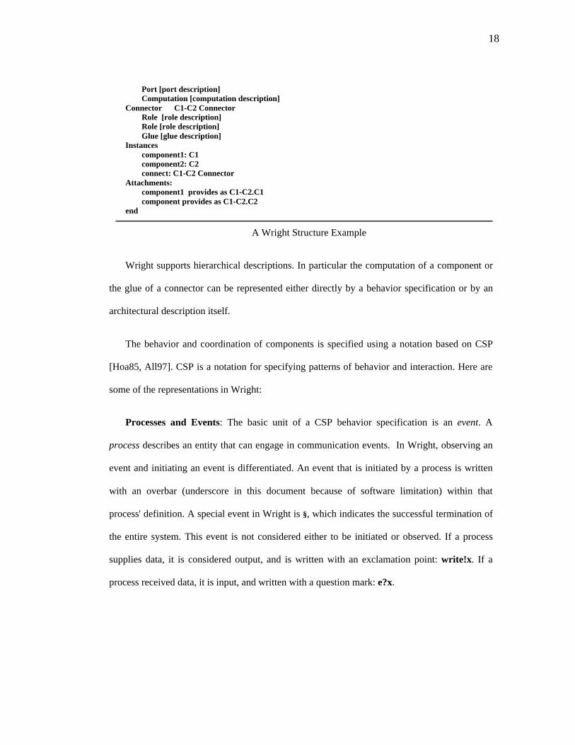
larger computation. A Wright structure example looks like this:
Component C1Port [port description]Computation [computation description]
Component C2
18
Port [port description]Computation [computation description]
Connector C1-C2 ConnectorRole [role description]Role [role description]Glue [glue description]
Instancescomponent1: C1component2: C2connect: C1-C2 Connector
Attachments:component1 provides as C1-C2.C1
component provides as C1-C2.C2end
A Wright Structure Example
Wright supports hierarchical descriptions. In particular the computation of a component or
the glue of a connector can be represented either directly by a behavior specification or by an
architectural description itself.
The behavior and coordination of components is specified using a notation based on CSP
[Hoa85, All97]. CSP is a notation for specifying patterns of behavior and interaction. Here are
some of the representations in Wright:
Processes and Events: The basic unit of a CSP behavior specification is an event. A
process describes an entity that can engage in communication events. In Wright, observing an
event and initiating an event is differentiated. An event that is initiated by a process is written
with an overbar (underscore in this document because of software limitation) within that
process' definition. A special event in Wright is §, which indicates the successful termination of
the entire system. This event is not considered either to be initiated or observed. If a process
supplies data, it is considered output, and is written with an exclamation point: write!x. If a
process received data, it is input, and written with a question mark: e?x.

19
Prefixing: Given a process P and an event e, the process e P is the process that first
engages in the event e and then behaviors as P.
Alternative ("external choice"): A process that can behave like P or Q, where the choice is
made by the environment, is denoted by the operator p. The process e P f Q is the
process that will behave as the process P if it first observes the event e and will behave as the
process Q if it first observes the event f. Because the behavior of the process is entirely
determined by what the environment does, this type of choice is called deterministic.
"Environment" refers to the other processes that interact with the process.
Decision ("internal choice"): A process that can behave like P or Q, where the choice is
made (non-deterministically) by the process itself, is denoted P Q. The process e P F
Q is the process that will either output e and then act as P or output f and then act as Q. The
process itself decides which choice to take without consulting the environment.
Sequence: The ";" operator combines two processes in sequence. P;Q is the process that
behaves as P until P terminates successfully and then behaves as Q.
Behavior patterns that occur over and over again can be described by naming particular
processes. P = e P. Named processes can also be introduced into other processes using
Where: f P where P = e P . This process does a single f and then repeats e over and over.
State is added to a process definition by adding subscripts to the name of a process: Pi is a
process with a single state variable, i. For example, P1 where Pi = count!i Pi+1 is a process
that counts : count!1, count!2, count!3, etc. For more than state variables, simply add
corresponding number of subscripts to the name of the process.
20
Pv = Q, when p(V) defines a process P over variables V only when the boolean expression
p(V) is true.
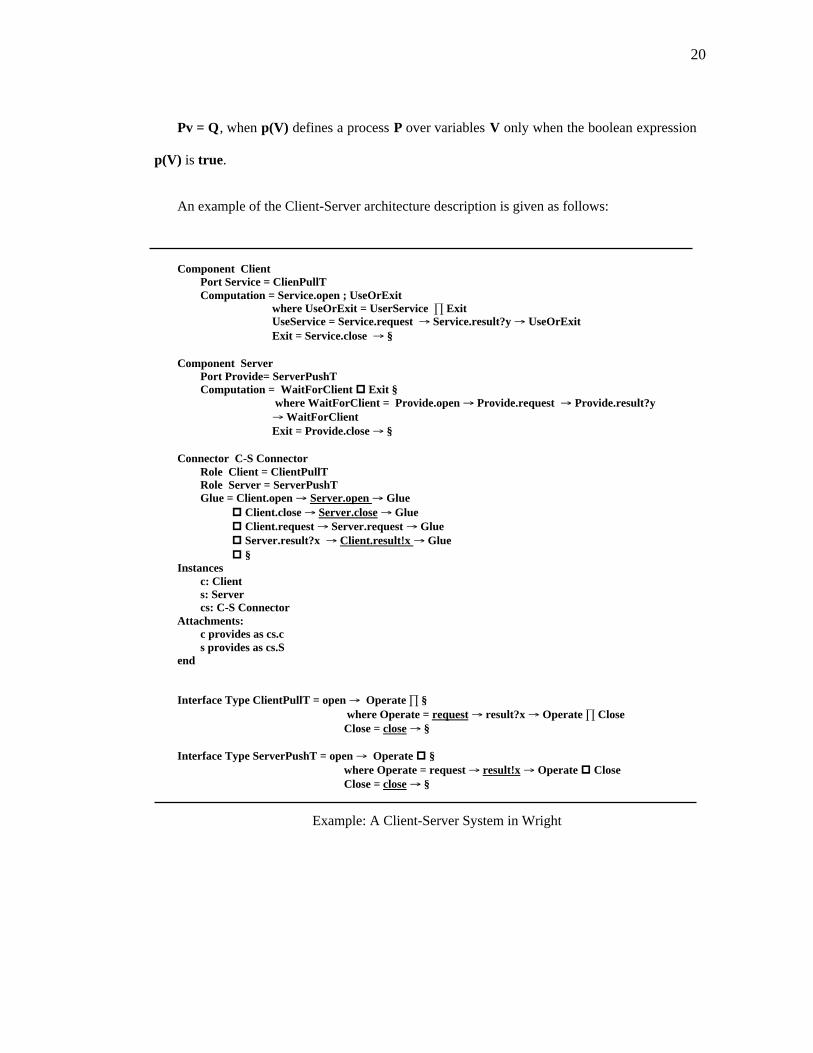
An example of the Client-Server architecture description is given as follows:
Component ClientPort Service = ClienPullTComputation = Service.open ; UseOrExit
where UseOrExit = UserService Exit UseService = Service.request Service.result?y UseOrExit Exit = Service.close §
Component ServerPort Provide= ServerPushTComputation = WaitForClient Exit §
where WaitForClient = Provide.open Provide.request Provide.result?y WaitForClient Exit = Provide.close §
Connector C-S ConnectorRole Client = ClientPullTRole Server = ServerPushTGlue = Client.open Server.open Glue Client.close Server.close Glue Client.request Server.request Glue Server.result?x Client.result!x Glue §
Instancesc: Clients: Servercs: C-S Connector
Attachments:c provides as cs.c
s provides as cs.Send
Interface Type ClientPullT = open Operate § where Operate = request result?x Operate Close
Close = close §
Interface Type ServerPushT = open Operate § where Operate = request result!x Operate Close
Close = close §
Example: A Client-Server System in Wright

21
In CSP and also in Wright, the use of the term "process" does not mean that the
implementation of the protocol would actually be carried out by a separate operating system
process. Processes are logical entities used as specification building blocks. Also event is not an
ordinary event, but has special rules associated with. See [ROS98] for details.
2.2 Petri Nets
Petri Nets have been introduced for modeling distributed systems because they give a
graph-theoretic representation of the communication and control patterns, and a mathematical
framework for analysis and validation [Peterson81, RT86, Jin94]. Petri Net modeling is
appealing for the following reasons:
- Petri Nets capture the precedence relations and structural interactions of concurrent and
asynchronous events. Petri Nets provide an integrated methodology, with well-
developed theoretical and analytical foundations for modeling complex systems.
- The graphical nature of Petri Nets helps to easily visualize the complexity of the
system.
- The mathematical representations of Petri Nets allow for quantitative analysis of
invariants, deadlock detection, resource utilization, throughput rate, effect of failures,
and real-time implementation.
- Petri Nets can be executed and can actually show the dynamics of the system. This
makes the Petri Nets a powerful modeling language.

22
A Petri Net is a bipartite directed graph: N= (P, T, I, O). There are two sets of nodes:
• P = {p1, ..., pn} is a finite set of places. Each place pi models a resource, a buffer, or a
condition. A place is depicted by a circle node.
• T = {t1, ..., tm} is a finite set of transitions. Each transition ti stands for a process, an
event, or an algorithm. A transition is represented by a bar node.
• The arcs that connect these nodes are directed and fixed. They can only connect a place
to a transition, or a transition to a place. They are given by: I : P × T -> {0,1}, O : P ×
T -> {0,1}. I is an input function that defines the set of directed arcs from P to T. I(p,t)
= 1 if the arc exists, I(p,t) = 0 otherwise. An arc from a place p to a transition t
indicates that the process t requires the availability of the resource p, the fulfillment of
the condition p, or the availability of information in the buffer p, in order to occur. O is
an output function that defines the set of directed arcs from T to P. O(p,t) = 1 if the arc
exists, O(p,t) = 0 otherwise. An arc from a transition t to a place p indicates that when
the process t is finished, it either enables the condition p, makes the resource p
available, or sends an item of information to the buffer p. Figure 2-1 shows a Petri Net.
Figure 2-1 A Petri Net Example
p1 p2
p3 p4
t1
t2
t3 p5

23
The set of places P, the set of transitions T, and the input and output functions that define
the arcs for this net are:
P = { p1, p2, p3, p4, p5} T = {t1, t2, t3}
I(p1, t1) = I(p2, t3) = I(p3, t2) = I(p4, t3) = 1, I(p, t) = 0 otherwise.
O(p2, t1) = O(p4, t 2) = O(p5, t3) = 1, O(p, t) = 0 otherwise.
Dynamics of Petri Net
A Petri Net can contain tokens. Tokens are depicted graphically by indistinguishable dots
(•), and reside in places. The existence of one or more tokens represents either the availability of
the resource, or the fulfillment of the condition, or the number of items of information in the
buffer. The distribution of tokens in the net is controlled by the transitions. A marking of a Petri
Net is a mapping M that assigns a non-negative integer (the number of tokens) to each place.
The number and position of tokens may change during the execution of a Petri Net. The tokens
are used to define the execution of a Petri Net.
A transition is enabled by a marking if and only if all of its input places contain at least one
token provided each input arc represents a single connection between the place and the
transition. Formally, M(p) > 0.
An enabled transition can fire. The firing of the transition corresponds to the execution of
the process or the algorithm. The dynamic behavior of the system is embedded in the changes of
the markings. When the firing takes place, a new marking is obtained by removing a token from
each input place and adding a token to each output place, M' is said to be reachable from M

24
after one firing: M’(p) = M(p) + #O(p,t) - #I(p,t). As an example, consider the Petri Net in
Figure 2-2 with the indicated marking.
M(p1) = M(p3) = 1; M(p4) = 2; M(p2) = M(p5) = 0.
Figure 2-2 A Petri Net with Marking
In Figure 2-2, if t1 fires, then the resulting marking is shown in Figure 2-3.
Figure 2-3 A Petri Net After Firing
Transitions t3 and t2 are now enabled. If t3 fires, the new marking is shown in Figure 2-4.
p1 p2
p3 p4
t1
t2
t3 p5
p1 p2
p3 p4
t1
t2
t3 p5

25
Figure 2-4 Petri Net after Second Firing
Mathematical representation of Petri Nets -- Linear Algebraic Approach
As with any other graphs, a Petri Net with n places and m transitions can be represented by
an n × m matrix C, the Incidence Matrix. The rows correspond to places, the columns
correspond to transitions. The cells are defined as follows:
• Cij = 1 if there is a directed arc from the j-th transition to the i-th place. "1" indicates
that the firing of the j-th transition adds one token to the i-th place.
• Cij = -1 if there is a directed arc from the i-th place to the j-th transition. "-1" indicates
that the firing of the j-th transition removes one token from the i-th place.
• Cij = 0 if there is no arc from the j-th transition to the i-th place.
For example, the incidence matrix of the net on Figure 2-1 is
t1 t2 t3
C =
-1 0 0 1 0 -1 0 -1 0 0 1 -1 0 0 1
p1p2p3p4p5
p1 p2
p3 p4
t1
t2
t3 p5
26
2.3 Software Testing
Software testing is directly concerned with software quality. The goal of testing is not to
show the absence of failures in the software, but rather shows the presence of failures and gives
the tester confidence on the software system. We may have different objectives for testing: to
see if the software works, to find errors, or to check consistency and etc. Beizer [Bei90] defines
six levels at which software testing occurs, unit test, module test, integration test, subsystem
test, system test and acceptance test. Unit and module testing analyzes the local behavior of
individual software blocks. Integration testing analyzes how individual block behaviors, and the
interactions among blocks, contribute to the global system behavior of the system without
regard to its decomposition. Subsystem testing refers to testing of coherent software subsystems
before integrating into the complete system. System testing has the particular purpose to
compare the software system to its original objectives, in particular validating whether the
software meets the functional and non-functional requirements. Acceptance testing gets the user
involved by asking if the user accepts the complete system.
Testing techniques can be categorized into two general approaches, black box and white
box. Black box testing approaches create test data without using any knowledge of the structure
of the software under test, whereas white box testing approaches explicitly use the program
structure to develop test data. Black box testing is usually based on the requirements,
specifications or design, while white box testing is usually based on the implementation in a
specific programming language. White box testing approaches are typically applied during unit
testing, and black box testing approaches are typically applied during integration and system
testing.
27
An important problem in software testing is deciding when to stop. Test cases are run on
test programs to find failures. Unfortunately, we cannot exhaustively search the entire domain
of the program (which in most cases is effectively infinite). Testing strategies may be
conveniently categorized by the goal they seek to achieve. Weyuker [Wey86] has characterized
these goals as adequacy criteria. Adequacy criteria are defined for testers to decide whether
software has been adequately tested for a specific testing criterion [FW88]. A testing criterion is
a rule or a set of rules that impose requirements on a set of test cases. Test engineers measure
the extent to which a criterion is satisfied in terms of coverage, which is the percentage of test
requirements that are satisfied. Test requirements are specific criteria that must be satisfied or
covered, e.g., reaching statements are the requirements for statement coverage in unit testing,
killing mutants are the requirements for mutation testing [DLS78], and executing definition/use
pairs are the requirements in data flow testing [FW88]. There are various ways to classify
adequacy criteria. One of the most common is by the source of information used to specify
testing requirements and in the measurement of test adequacy. Hence, an adequacy criterion can
be specification-based or program-based.
Most current testing approaches are either based on the implementation or structural
information of the system or based on a requirement specification or system design, yet most
high level design representations and requirement specifications are not formal enough to do
this in an automated fashion. With the advent of formal architecture specification, however,
architecture based test criteria can be defined based on the system properties that an ADL
describes. This would support algorithmically defining test data to cover the architecture and
automatically developing architectural test plans – testing at the architecture level.

28
2.4 Issues in Software Architecture-Based Testing
As in any other testing techniques, we need to know what to test at the software architecture
level and therefore we can define testing requirements at this level. Most unit level testing
techniques use program structure to define test adequacy criterion, for instance, conditions
(control flow) or variable define-use pairs (data flow). At the integration and system testing
level, the predominant form for defining testing criteria is based on definition/use bindings
[PN86], where each module defines or provides a set of facilities that are available to the uses or
requires by other modules. Coupling-based testing techniques [JO98] and inter-procedural
testing techniques [HR94] are such examples. These techniques use information from
underlying implementation languages such as procedure calls or data sharing which means the
software must already be complete. But software architecture is beyond this level [AG94c].
Software architecture focuses on the interaction between components, and normally the view of
interaction is implementation language independent. Therefore, set up testing criteria that uses
traditional implementation-based structure information may not be possible at the software
architecture level. So interaction between components will be our major focus when testing.
Presentation of interaction properties of a software architecture becomes the key point.
As described in the previous section, ADLs are used to give formal definitions to software
architectures. But current ADLs have different focuses on different aspects of software
architecture [Med97, Cle96a]. For instance, Rapide is a general-purpose event-based description
language and it allows modeling of component interfaces and their external behavior, while
Wright focuses on formalizing the semantics of connections. Medvidovic and Clements
[Med97, Cle96a] both give surveys on these ADLs and try to summarize what properties need

29
to be described in an ADL. In the proposed research, we need to extract the general properties
that are important to software testing. These general properties will be useful both in testing
software architectures directly as well as in software conformance testing. Once we know what
we need to test, we need to define test requirements on these properties, therefore we can define
general testing criteria at the software architecture level. In summary, the major issues in
software architecture testing are:
• what are the general properties that are important for testing at this level?
• based on these general properties, what test requirements can be formulated?
• what general testing criteria can be defined at this level?
2.5 General Properties to Be Analyzed and Tested at the Architectural Level
An initial step in developing new testing methods is to enumerate the kinds of problems that
can exist. We have developed some preliminary architectural testing properties. It should be
emphasized that this list is tentative and work is ongoing to refine the set of properties to test for
at this level. In the list of properties, a conflict occurs when rules, constraints or semantics
cannot both be satisfied at the same time. In general, deadlock implies that a process does not
participate in any events, but has not yet terminated successfully. A process is deadlock free if it
can never go into a deadlock state.
1. Component Consistency Requirements: Semantics, constraints and interfaces can be
associated with components. They should be consistent with respect to each other and this

30
consistency needs to be considered at the architecture level. Interfaces have types as well as
data and control constraints.
• Component constraints and semantics should have no conflicts.
• Component constraints and semantics should be deadlock free.
• Component constraints and semantics should have no conflicts with the component
interface constraints.
2. Connector Consistency Requirements: A connector also contains interfaces, semantics, and
constraints that need to be consistent. Interfaces have types as well as data and control
constraints.
• Connector constraints and semantics should have no conflicts.
• Connector constraints and semantics should be deadlock free.
• Connector constraints and semantics should have no conflicts with the associated
connector interfaces constraints.
3. Component-Connector Compatibility Requirements: Component interfaces are associated
with connector interfaces to enable interactions. Informally, compatibility means that a
component interface behaves in a manner that is consistent with assumptions made by the
connector.
• Component interfaces should be compatible with the associated connector interfaces.
• For some compatibility requirements, it must be determined whether the
component/connector relationship is deadlock free.
4. Configuration Requirements: The configuration of a software architecture should be tested
against several test requirements. An initiation state is the "start state", the state that the

31
system is initially in. There are explicit data flows through the architecture of the system; a
data element is given a value (defined) in its source component and the value is used in a
target component. There are also explicit control flows; each architecture element has one or
more designated next element. This transfer of execution could be between states in a
component, through connectors, or across components.
• Data Flow Reachability: A data element should be able to reach its designated target
component from its source component through the connectors. The data element should
reach the target component without having its value modified.
• Control Flow Reachability: Every architecture element should be able to reach its
designated next element.
• Connectivity: A component or connector interface with either no next element or no
previous element is said to be "dangling". Dangling components and connector
interfaces could indicate potential problems.
• Interactions that in isolation are deadlock free can interact in such a way as to cause a
deadlock situation. It should be the case that the system is deadlock free.
5. Style Restriction Requirement: The architecture style being used imposes some constraints
on the software configuration. The system being used must satisfy those constraints.
System-level tests derived from architectures can validate that the software implements the
architecture correctly and help to verify the architecture. If the architecture is sufficiently
descriptive, then the tests should be effective at finding problems in the implementation. In this
dissertation, we only discuss test case generation technique, analysis and evaluation of the ADL
specification is not in the scope of this research.

32
2.6 Related Work
Related work for this research covers the following areas: ADL survey, formal definition of
software architecture, architecture-based dependency analysis and testing, component adequacy
testing and mismatches of components.
2.6.1 ADL Classification and Survey
Medvidovic [Med97] gives a survey of most of the current ADLs and summarizes some
software architecture properties that current ADLs can describe. This survey classifies and
compares properties in components, connections, and configurations and how they are
represented in these ADLs. It makes an attempt to answer the question of what an ADL is and
why, and how it compares to other ADLs. Such information is very important for understanding
current status of ADLs. Even though the architectural properties these ADLs describe are not
specific for testing purpose, they help us understand and pick the properties to test.
2.6.2 Formal definition of Software Architecture
Allen [All97] shows that an Architecture Description Language based on a formal, abstract
model of system behavior can provide a practical way to describe and analyze software
architectures and architectural styles. He introduces Wright, an architectural description
language based on the formal description of the abstract behavior of architectural components
and connectors. Wright uses explicit, independent connector types as interaction patterns, it
describes the abstract behavior of components using a CSP-like notation, and styles can be
characterizes by using predicates over system instances. His work also shows some static
checks to determine the consistency and completeness of an architectural specification.

33
2.6.3 Correctness and Composition of Software Architectures
Moriconi and Qian [MORI94] discuss correctness and composition of software
architectures. In their paper, they provide a formal criterion for proving that one architecture
implements another architecture, even if they are described in different architectural styles.
They use first-order logic for the definition of both configuration and style structures, and
provide a specific model of style-based refinement of configurations.
2.6.4 Architecture-level Dependency Analysis & Testing
Richardson and Wolf present their research in architecture-based dependency analysis and
testing [RW96, SRW97, SRW98]. The Chemical Abstract Machine (CHAM) model is used to
represent software architectures. The CHAM for a software architecture defines molecules
(elements), solutions (combinations of elements), and transformation rules that specify how
solutions evolve. Dependency analysis is based on structural relationships (textual inclusion,
import/export, inheritance) and behavioral relationships (temporal, state-based, causal,
input/output). The structural dependencies allow one to locate source specifications that
contribute to the description of some state or interaction. The behavioral dependencies allow
one to relate states or interactions to other states or interactions. These relations are recorded in
a table for dependency analysis. Testing criteria are defined based on the CHAM model. For
example, all-data-elements requires that all data defined in the architecture are communicated
(for each data element d, at least one solution contains a molecule involving d), and all-
processing-elements requires that all processing elements are executed (for each processing
element p, at least on solution contains a molecule involving p). However it has been argued
[All97] that CHAM describes the structure and abstract behavior of a single configuration,
rather than a class of systems. Medvidovic [Med97] also argues that even though CHAM can

34
be used effectively to prove certain properties of architectures, the interface topology is implicit
in the solution and transformation rules. So this does not meet the requirements to be an ADL.
2.6.5 Component-based Testing
Rosebblum [Rosen00, Rosen97] initiates the development of a component-based software
testing theory. Two concepts were defined: the concept of C-adequate-for-P for adequate unit
testing of a component and the concept C-adequate-on-M for adequate integration testing of a
component-based system. This technique views testing of component-based software as both a
unit testing problem for program M, and an integration testing problem for program P
containing M. The unit-testing viewpoint requires the developer of M to test M with criterion C
and to carry out the testing with a test set that is C-adequate-for-P. The integration testing
viewpoint requires the developer of P to test P with a test set that is C-adequate-on-M. If the
test adequacy criteria being used are code coverage criteria, then satisfaction of these
requirements can be checked. A formal model of component-based software was defined, and
the model was used to formally define a notion of test adequacy for component-based systems.
The notion of component as used in this technique corresponds to a general object-oriented
notion of a component. A component M encapsulates some state and provides a well-defined
interface that strictly governs access to the state by other parts of a system containing the
component. The interface is viewed as a set of methods or operations that can be applied to the
component. Generally speaking, this technique is at the integration level rather than at the
architectural level and it is also based on the completeness of the implementation. This work is
different from the testing technique proposed in this dissertation.

35
Chapter 3 Software Architecture-based Testing Technique
Traditionally, software system level testing has been based on informal, manual, and ad-hoc
analyses of the system requirements. This informality may make it hard to distinguish different
levels of abstraction throughout the process and thus may lead to inconsistent testing results and
lack of repeatability in the process. Formalized software architecture description languages
represent significant opportunities for testing because they formally describe how the software
system is expected to behave in a high level view that allows test engineers to focus on the
overall system structure, and also in a form that can be handled automatically.
This chapter discusses a new software testing technique at the software architecture level.
As we have discussed in Chapter 1, the overall topology is presented in three parts: Testing
Techniques for General ADLs, Applying the Technique to a Specific ADL, and Tests for an
Implementation. This chapter focuses on presenting a testing technique for general ADLs,
shown in Figure 3-1. We introduce a graphical representation Interface Connectivity Graph
(ICG) and the construction of an ICG, then define the testing requirements and testing criteria
defined based on the ICG. The testing criteria may serve as guidelines for testers to decide when
to stop testing. Test coverage measurement is also discussed at the end of this chapter.
We use the following definitions here and after this chapter. Test requirements are specific
things that must be satisfied. For example, reaching statements are the requirements for
statement coverage, and killing mutants are the requirements for mutation testing. A testing

36
criterion is a rule or a collection of rules that imposes requirements on a set of test cases.
Testers ensure the extent to which a criterion is satisfied in terms of coverage, which is the
percentage of requirements that are satisfied.
Figure 3-1 Testing Technique Procedures
3.1 Basic Definitions
To make architecture-based testing a manageable process, testing must be guided by the
definition of the architecture. As we have discussed, software architecture must be specified
using its own specification languages and analysis techniques in order to achieve benefits. A
large number of ADLs have been proposed, each of which specifies a particular approach and
specifies certain aspects of a software architecture. Even though there is no unique definition of
what an ADL should describe, we need to understand what software architecture aspects an
ADL should describe and start testing those aspects.
Before we discuss the general architectural aspects that need to be tested, we first define
some terms taken from Medvidovic's paper [Med97]. We view software architecture as
Testing Technique for General ADLs
GeneralADL
Rules ForConstructing an ICG
TestingCriteria
Part 1
Applications in Chapter 4

37
components, connectors and configuration. For each component and connector, its interface,
types, constraints and semantics are defined.
A Component's Interface is a set of interaction points between this component and other
components that this component interacts with. It specifies the services (messages, operations,
and variables) a component provides. Interfaces in ADLs are represented as either ports (as in
Wright) or constituents (as in Rapide). ADLs support reuse by modeling abstract components as
types and instantiating them multiple times in an architectural specification. Abstract component
types can also be parameterized to further facilitate reuse. Component Semantics is a description
of component behavior; it enables analysis, constraint enforcement, and mappings of
architectures across levels of abstraction. Component Constraints is a property of or assertion
about a system or one of its parts. Constraints are specified to ensure adherence to intended
component uses, enforce usage boundaries, and establish intra-component dependencies. A
connector's interface is a set of interaction points between it and the components attached to it.
It enables proper connectivity of components and their communication in a software
architecture. Architecture-level communication is often expressed with complex protocols. To
abstract away these protocols and make them reusable, ADLs should model connectors as
Connector Types . Connector Semantics provides connector protocol and transaction semantics
so as to be able to perform analyses of component interactions, consistent refinements across
levels of abstraction, and enforcement of interconnection and communication constraints. Not
every ADL models connector semantics. Connector Constraints specifies constraints to ensure
adherence to interaction protocols, establish intra-connector dependencies, and enforce usage
boundaries. In order to describe software systems at different levels of detail, architecture
configurations Compositionability supports the situations where a software architecture may

38
become a mere component in a bigger architecture or vise versa. Architecture Configurations
Constraints describe desired dependencies among components and connectors in a
configuration.
Figure 3-2 shows these aspects in a software architecture. These architecture aspects will be
used for the software architecture-based testing. From now on, we name components,
connectors, interfaces of components and connectors as the architecture units. Other
architecture aspects such as constraints and semantics will be used to define possible
relationships among these architecture units. Configuration will be considered as the
instantiation of the architecture units. When it comes to a specific ADL description, it may not
have all these aspects defined explicitly or defined at all. For instance, Rapide [LV95] does not
explicitly describe a connector, it has no constraints or semantics for the connector. So when
applying architecture-based testing technique to a specific ADL, we will only consider those
aspects that are described in the ADL, therefore, the application of this testing technique will
vary based on the ADL used.
Figure 3-2 Architecture Aspects
componentconnector
component
constraints
semantics
constraints
semantics
constraints
semantics
interfacestypes types typesinterfaces

39
3.2 Architecture-based Testing Technique for General ADLs
Relations among architecture units are the key factors in a software architecture description,
they define the behaviors and connectivities among software components via connectors. Our
software architecture-based testing technique focuses on testing the relations among architecture
components. Therefore, we define relations among architecture units as software architecture
relations. The technique requires that tests cover certain architecture relations among
components and connectors or inside a component and a connector. These architecture relations
are based on the possible bindings: data transfer, control transfer, and execution ordering rules.
Formal descriptions of these relations are defined in the next section. The underlying premise of
the architecture-based testing criteria is that to achieve confidence in the architecture relations
between architecture components and connectors, it must be ensured that all the existing
architecture relations be covered in the test. Because this technique is limited to the architecture
description, it is only concerned with relations at the architecture level, not with detail design or
implementation level, but they can be extended to the software design or implementation level.
3.2.1 What Needs to be Tested at the Architecture Level – Testing Requirements
Given architecture relations among components, interfaces, and connectors, software
architecture testing needs to focus on testing the following aspects:
1. Testing component to connector connectivity: this tests the connectivity and
compatibility from a component interface to a connector interface.
2. Testing connector to component connectivity: this tests the connectivity and
compatibility from a connector interface to a component interface.

40
3. Testing component internal interfaces: this tests the possible data transfer, control
transfer, and ordering relations among the interfaces inside a component.
4. Testing connector internal interfaces: this tests the possible data transfer, control
transfer, and ordering relations among the interfaces inside a connector.
5. Testing direct component to component connectivity: this tests the connection of two
components through a connector.
6. Testing indirect component to component connectivity: this tests a subset of
components and connectors that are indirectly data or control related.
7. Testing whole structure connectivity: this tests the overall architecture structure
connectivity. All connections among components, connectors and all internal
connections are tested.
3.2.2 Architecture-based Testing Concepts
Testing at the unit level focuses on relations on program units, such as statements, variables,
or conditions. Testing at the architecture level should focus on the architecture relations of the
architecture units specified by a specific ADL description. This section defines some concepts
for the architecture relations. To visualize the architecture relations, a graphical representation
of the architecture is introduced in this section, we then can derive testing requirements and
testing criteria based on this graphical representation.

41
3.2.2.1 The Interface Connectivity Graph (ICG)
Testing adequacy criteria help to tell testers when testing is enough and when to stop.
Graphical representations have long been used to help to visualize the definition of testing
criteria. For instance, data flow diagrams, control flow diagrams, state transition diagrams, etc.,
have all been used in defining testing criteria and in generating testing cases. Therefore, we
introduce graphical representations to help visualize our architecture-based testing technique.
The Interface Connectivity Graph (ICG) represents the connectivity relationships between
components and connectors as well as relations inside a component and a connector.
An ICG is composed of a set of components (visually as rectangular boxes), component
interfaces (clear circles on the edge of the component boxes), connectors (round boxes),
connector interfaces (shaded circles on the edge of the connector boxes), connections between
connectors and components (solid arrows), and connections inside components or connectors
(dash-line arrows).
Definition 3.1 Architecture Interface Connectivity Graph (ICG)
Given a software architecture defined by a specific ADL, the architecture Interface
Connectivity Graph (ICG) is defined as:
ICG = (N, C, N_Interf, C_Interf, N_Ex_arc, C_Ex_arc, N_In_arc, C_In_arc),
• N = {N1, N2, … Nn}, a finite set of components
• C = {C1, C2, … Cm}, a finite set of connectors
• N_Interf = {N1.interf1, … N1.interfs, … Nn.interf1, … Nn.interfx}, a finite set of
component interfaces
• C_Interf = {C1.interf1, … Cm.interft), a finite set of connector interfaces

42
• N_Ex_arc is defined as (N × C) → {0, 1}, if N_Ex_arc(n, c) = 1, then the arc exists,
there is a connection between the component interface to a connector interface,
otherwise the arc does not exist
• C_Ex_arc is defined as (C × N) → {0, 1}, if C_Ex_arc(n, c) = 1, then there is an arc
between a connector to a component interface, otherwise the arc does not exist
Because C_Ex_arc and N_Ex_arc contain arcs that connect components and
connectors, they are viewed as the external arcs. Internal arcs represent the connections
between interfaces of one component or they represent the connections between interfaces
of one connector. Internal arcs are defined as follows.
• N_Inter_arc = (C_Interf × N_Interf) → {0, 1}, if N_In_arc (n.interf1, n.interf2) = 1, then
there is a connection between n.interf1 and n.interf2, otherwise there is no such an arc
• C_Inter_arc = (C_Interf × C_Interf) → {0, 1}. If C_Inter_arc (c.interf1, c.interf2) = 1,
then there is an arc c.interf1 and c.interf2. Otherwise, there is no such an arc
As an example, consider a software system that consists of two Graphical User Interface
(GUI) components that acquire data from the server component. Server contains an internal
database that has to synchronize its data with data processed in Sync component. The data
contained in the internal database in Server needs to be updated by the DataStore component,
where it processes the data and output the data to Server. The ICG of the system is shown in
Figure 3-3.

43
Figure 3-3 An ICG Example
In this example, there are five components and four connectors and a number of arcs
connecting them. Details are given as follows:
N = {GUI1, GUI2, Server, DataStore, Sync}
C = {CS1, CS2, SD1, SD2}
N_Interf = {GUI1.i1, GUI2.i1, Server.i1, Server.i2, Server.i3, Server.i4, Sync.i1,
DataStore.i1}
C_Interf = {CS1.i1, CS1.i2, CS2.i1, CS2.i2, SD1.i1, SD1.i2, SD2.i1, SD2.i2}
N_Ex_arc = {a1, a4, a6, a7, a10, a12}
C_Ex_arc = {a2, a3, a5, a8, a9, a11}
N_In_arc = {b7}
C_In_arc = {b1, b2, b3, b4, b5, b6}
GUI 1 CS1 Server SD1DataStore
a1 a2
a3 a4
a5 a6b1
b2
b5i1
i1 i2
i1 i2
i1 i2 i1
GUI 2
i1
CS2
b3
b4i1 i2
Sync
i1
SD2
i1
i2
i3 i4
a7
a8
a9
a10 a11
a12b6
b7

44
Definition 3.2 Data Structure Representation of an ICG -- ICG Incidence Matrix
As with any other graphs, an ICG with n total component interfaces and m total
connector interfaces can be represented by an (n+m) (n+m) matrix M, the ICG
Incidence Matrix . The rows correspond to the component interfaces and the connector
interfaces, the columns correspond to the component interfaces and the connector
interfaces. The cells are defined as follows:
• Mij = 1 if there is a directed arc from the j-th interface to the i-th interface.
• Mij = -1 if there is a directed arc from the i-th interface to the j-th interface.
• Mij = 0 if there is no arc between the j-th interface and the i-th interface.
3.2.2.2 Architecture Relations
Testing at all levels focuses on relations among program units and aims to generate test
cases to cover these relations. Testing criteria are usually defined to cover certain relations
among program components. For instance, in unit level data flowing testing [FW88], variable
definition-usage defines one type of data flow relation inside a program, covering all the def-use
pairs becomes one of the data flow testing criteria. At subsystem level, coupling-based testing
[JO98] defines coupling relations between two software components, covering different
coupling relations therefore satisfies different types of coupling-based testing criteria. At the
software architecture level, we need to first define general architecture relations for a software
architecture described by an ADL description, then derive testing requirements and criteria
based on the architecture relation coverage. It can be seen that finding the right relations
provides a good foundation for deriving good testing requirements and testing criteria.
45
Definition 3.3 Component Internal Transfer Relation
The component internal transfer relation defines the possible data transfer or control
transfer relations between two interfaces inside a component.
N_Internal_Transfer_Relation(N.interf1, N.interf2): (N_Interf × N_Interf) → {0, 1}== 1 if
for a component N, there is a data or control transferred from N.interf1 to N.interf2,
otherwise 0. This relation is non-reflexive, non-symmetric, and it is not transitive.
For instance, if component A has two interfaces p1 and p2, if interface p1 closes, then
interface p2 closes, this is a control relation between the two interfaces. If interface p1 reads
data and the same data is used by interface p2, then there is a data relation between these
two interfaces. These are considered to be component internal transfer relations.
The component internal transfer relation can be extracted from the architecture
description in a specific ADL description. Note that we only discuss these types of
relationship at the ADL description level, any possible relationships that may occur at the
implementation level are not considered at this level.
Definition 3.4 Component Internal Ordering Relation
If the interfaces of a component have to behave based on some execution ordering rules,
either be in parallet or sequential, then there is an ordering relation between the component
interfaces. If two or more interfaces can occur in any arbitrary order, then there is no
specific ordering relation between the interfaces. This is represented as
Component_Internal_Ordering_Relation(N.interf1, N.interface2): (N_Interf × N_Interf)
→ {0, 1}== 1 if N.interf1, N.interface2 have to follow certain execution ordering rules.

46
Otherwise 0. This ordering relation is non-reflexive, but is symmetric and transitive.
Interface ordering rules contains three types of orderings:
1) (p1 | p2): interface p1 has a data/control transfer to interface p2
2) (p1 // p2): interface p1 and p2 runs in parallel
3) (p1 => p2): interface p2 runs after p1 finishes processing
Definition 3.5 Component Internal Relation
Component_Internal_Relation(N1.interf1,N1.interf2): (N_Interf × N_Interf) → {0, 1}==
1 if (Component_Internal_Transfer_Relation(N1.interf1, N1.interf2) == 1 or
Component_Internal_Time_Relation(N1.interf1,N1.interf2) == 1), otherwise (N_Interf ×
N_Interf) → {0, 1}== 0.
Note that ordering rules in an ADL description may be represented as constraints or
implicitly described as part of the component behavior. For instance, in Wright, concurrent
processing of each interface can be described by constraints.
Definition 3.6 Connector Internal Transfer Relation
The connector internal transfer relation defines the possible data input/output or control
pass relations among interfaces inside a connector. Connector_Internal_Transfer_Relation
(C.interf1, C.interf2): (C_Interf × C_Interf) → {0, 1}== 1 if for a connector C, there is a
data or control transfer from C.interf1 to C.interf2, otherwise 0. This relation is non-
reflexive, non-symmetric and non-transitive.

47
Note that some ADLs may not have an explicit description on connectors or their
behavior. A detailed classification and survey can be found in Medvidovic's paper [Med97].
Definition 3.7 Connector Internal Ordering Relation
If the interfaces of a connector have to behave based on some ordering rules, the ordering
rules requires that the interfaces must run either in parallel or sequentially, then there is an
ordering relation among the connector interfaces. If two interfaces can occur at any
arbitrary order, then there is no specific ordering relation between the two interfaces. This is
represented as
Connector_Internal_Ordering_Relation(C.interf1, C.interface2): (C_Interf × C_Interf) →
{0, 1}== 1 if such ordering relation exists, 0 otherwise. This relation is non-reflexive, but is
symmetric and transitive.
Definition 3.8 Connector Internal Relation
A connector internal relation Connector_Internal_Relation(C.interf1, C.interf 2): (C_Interf
× C_Interf) → {0, 1}== 1 if Connctor_Internal_Data_Relation(C.interf1, C.interf2) == 1 or
Connector_Internal_Ordering_Relation (C.interf1, C.interf2) == 1, otherwise 0.
Again, some ADLs may not have a description on connector, therefore no connector
internal ordering restriction is given.

48
Definition 3.9 Component and Connector Relation
N_C_Relation(N.interf1, C.interf1): (N_Interf × C_Interf) → {0, 1}== 1 if an interface of a
component is associated with an interface of a connector, 0 otherwise. This relation is non-
reflexive, non-symmetric, and non-transitive.
Definition 3.10 Connector and Component Relation
C_N_Relation(C.interf1, N.interface1): (C_Interf × N_Interf) → {0, 1}== 1 if an interface
of one connector is associated with an interface of a component, 0 otherwise. This relation
is non-reflexive, non-symmetric, and non-transitive.
Definition 3.11 Direct Component Relation
Direct_Component_Relation (N1.interf1, N2.interf2): (N_Interf × C_Interf × C_Interf ×
N_Interf) → {0, 1}== 1 if N_C_Relation(N1.interf1, C1.interf1) == 1 and
C_N_Relation(C1.interf2, N2.interf2) == 1 and Connector_Internal_Relation(C1.interf1,
C2.interf2) ==1, 0 otherwise. This relation is reflexive, symmetric, but non-transitive.
Definition 3.12 Indirect Component Relation
If component N1, N2 has direction relation Direct_Compoent_Relation(N1.interf1,
C1.interf1, C1.interf2, N2.interf1) == 1 and component N2 and N3 has a direction relation
Direct_Component_Relation(N2.interf2, C2.interf1, C2.interf2, N3.interf2) == 1, also, if
Component_Internal_Relation(N2.interf1, N2.interf1) == 1, then
Indirect_Component_Relation(N1.interf1, C1.interf1, C1.interf2, N2.interf2, C2.interf1,
C2.interf2, N3.interf1): (N_Interf × C_Interf × C_Interf × N_Interf × C_Interf × C_Interf ×

49
N_Interf) → {0, 1}== 1, 0 otherwise. This relation is non-reflexive, non-symmetric, but is
transitive.
Definition 3.13 Initiation Point and Called Point
If Direct_Component_Relation(N1.interf1, C1.interf1, C1.interf2, N2.interf2) == 1, the
component interface that initiates the whole connection process is called an initiation point.
Every other component interface is called the called point.
To summarize, the following architecture relations are defined in this section. These
architecture relations will be used in defining the testing requirements and testing paths in
section 3.2.3.
• Component Internal Relation:
Component_Internal_Relation(N1.interf1, N1.interf2)
• Component Internal Transfer Relation:
Component_Internal_Transfer_Relation(N.interf1, N.interf2)
• Component Internal Ordering Relation
Component_Internal_Ordering_Relation(N.interf1, N.interf2)
• Connector Internal Relation:
Connector_Internal_Relation(C.interf1, C.interf2)
• Connector Internal Transfer Relation:
Connector_Internal_Transfer_Relation(C.interf1, C.interf2)
• Connector Internal Ordering Relation:
Connector_Internal_Odering_Relation(C.interf1, C.interf2)
• Component and Connector Relation:
50
N_C_Relation(N.interf1, C.interf1)
• Connector and Component Relation:
C_N_Relation(C.interf1, N.interf1)
• Direct Component Relation:
Direct_Component_Relation(N1.interf1, C1.interf1, C1.interf2, N2.interf1)
• Indirect Component Relation:
Indirect_Component_Relation(N1.interf1, C1.interf1, C1.interf2, N2.interf2,
C2.interf1, C2.interf2, N3.interf1)
Example ICG Architecture Relations and Paths
Given the ICG shown in Figure 3-3, assume that the Server component has to run first,
then the Server has to get information from the DatatStore and Sync components before the
Server can send out information through its ports Server.i1 and Server.i2. Both of the two
GUI components have to make requests to the Server and wait for responses back from the
Server. The following shows the ICG architecture relations. To make it simple to read and
understand, we use paths to represent these architecture relations.
Component Internal Transfer Relation:
• {Server(b7)} – There is only one transfer relation for all the components in Figure 3-3.
Component Internal Ordering Relation:
• {Sequence(Server(i2 // i4), Server(i1 // i3)} – In Server component, its port i2 and i4 and
run in parallel or independently, ports i1 and i3 can run in parallel, but either port i2 or i4
has to run before port i1 or i3 can run.

51
Component Internal Relation:
• {Server(b7), Sequence(Server(i2 // i4), Server(i1// i3)}
Connector Internal Transfer Relation:
• {GUI1(b1, b2), GUI2(b3, b4), SD1(b5), SD2(b6)}
Connector Internal Ordering Relation:
• {Sequence(CS1(b1), CS1(b2)), Sequence(CS2(b3), CS2(b4))} – Request first before
receiving response
Connector Internal Relation:
• {GUI1(b1, b2), GUI2(b3, b4), SD1(b5), SD2(b6), Sequence(CS1(b1), CS1(b2)),
Sequence(CS2(b3), CS2(b4)) }
Component and Connector Relation:
• {a1, a7, a4, a9, a6, a12}
Connector and Component Relation:
• {a3, a8, a4, a10, a5, a11}
Direct Component Relation:
• {(GUI1(i1), CS1(i1), CS1(i2), Server(i1)), -- GUI1-CS1-Server
(GUI2(i1), CS2(i1), CS2(i2), Server(i2)), - - GUI2-CS2-Server
(DataStore(i1), SD1(i2), SD1(i1), Server(i2)), -- DataStore-SD1-Server
(Srnc(i1), SD2(i2), SD2(i1), Server(i4)) } -- Sync-SD2-Server
Indirect Component Relation:
None in this case.

52
3.2.3 Architecture-based Testing Path Definitions
Before testing coverage criteria are defined, we need to formally define what needs to be
covered at the architecture level. These were informally discussed in section 3.2.1, we now
formally define the connectivities that need to be covered. An architecture-based testing path is
defined based on the ICG of a software architecture, it is a path between two interfaces (either
component interfaces or connector interfaces) from an initiation point to a called point and it
covers certain architecture relations so as to satisfy certain architecture-based testing
requirements. Because these testing paths are defined at the ICG level, they may appear only as
some simple edges in an ICG, but when it comes to a specific ADL description, more detailed
behavioral and design information need to be included to extend these edges at that level. This
is what we defined as part two of the overall testing technique, and it is presented Chapter 4.
Types of architecture-based testing paths are now defined, first informally, then formally.
1. Component internal transfer path
Given a component N, there is a Component internal data path if there is a
Component_Internal_Data_Relation(N.interf1, N.interf2) between the two interfaces.
This path is defined formally as:
Component_Internal_Transfer_Path = {(i, j) | i ∈ N_Interf, j ∈ N_Interf, and
Component_Internal_Transfer_Relation(i, j) == 1}
For example, b2 in Figure 3-4 is an Component_Internal_Transfter_Path.
Figure 3-4 An Example of Component_Internal_Transfer_Path
N1
i1 i2
b1

53
2. Component internal ordering rules
Given a component N, if any interface of N has an ordering relation, then there must
be a rule or set of rules for this ordering relation. This path is defined formally as:
Component_Internal_Ordering_Rule = {order_rules(i, j) | i ∈ N_Interf, j ∈ N_Interf,
and Component_Internal_Ordering_Relation(i, j) == 1}
For example, component N1 has three ordering rules as shown in Figure 3-5: i1 has
data/control transfer to i2; i2 and i3 are running in parallel; i3 interface runs after
interface i1 runs.
Figure 3-5 An Example of Component Internal Ordering Rules
3. Connector internal transfer path
Given a connector C, there is a path for Connector_Internal_Transfer_Relation
(C.interf1, C.interf2) between C.interf1 to C.interf2. This path is defined formally as:
Connector_Internal_Transfer_Path = {(i, j) | i ∈ C_Interf, j ∈ C_Interf, and
Connector_Internal_Data_Relation(i, j) == 1}
b1 in Figure 3-6 is a Connector_Internal_Transfter_Path.
Figure 3-6 An Example o f Connector_Internal_Transfter_Path
C1b1
i1 i2
N1
i1
i2
i3
Ordering rules:1. (i1 | i2)2. (i2 // i3)3. (i1 => i3)
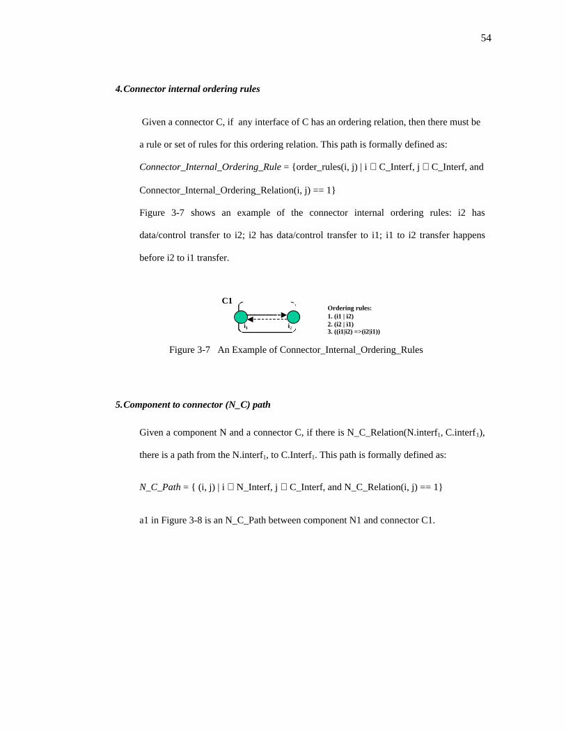
54
4. Connector internal ordering rules
Given a connector C, if any interface of C has an ordering relation, then there must be
a rule or set of rules for this ordering relation. This path is formally defined as:
Connector_Internal_Ordering_Rule = {order_rules(i, j) | i ∈ C_Interf, j ∈ C_Interf, and
Connector_Internal_Ordering_Relation(i, j) == 1}
Figure 3-7 shows an example of the connector internal ordering rules: i2 has
data/control transfer to i2; i2 has data/control transfer to i1; i1 to i2 transfer happens
before i2 to i1 transfer.
Figure 3-7 An Example of Connector_Internal_Ordering_Rules
5. Component to connector (N_C) path
Given a component N and a connector C, if there is N_C_Relation(N.interf1, C.interf1),
there is a path from the N.interf1, to C.Interf1. This path is formally defined as:
N_C_Path = { (i, j) | i ∈ N_Interf, j ∈ C_Interf, and N_C_Relation(i, j) == 1}
a1 in Figure 3-8 is an N_C_Path between component N1 and connector C1.
Ordering rules:1. (i1 | i2)2. (i2 | i1)3. ((i1|i2) =>(i2|i1))
i1 i2
C1

55
Figure 3-8 An Example of N_C_Path
6. Connector to component (C_N) path
Given a component N and a connector C, if there is a C_N_Relation(C.interf1,
N.interf1), there is a path from C.interf1 to N.interf1. This path is formally defined as:
C_N_Path = { (i, j) | i ∈ C_Interf, j ∈ N_Interf, and C_N_Relation(i, j) == 1}
a2 in Figure 3-9 is a C_N_Path between connector C1 and component N2.
Figure 3-9 An Example of C_N_Path
7. Direct component to component path
Given two components N1 and N2, and a connector C1, if there is an architecture
relation Direct_Component_Relation(N1.interf1,C1.nterf1) and a
C_N_Relation(C1.interf2, N2.Interf1), there is a path from N1.interf1 to C1.interf1 to
C1.interf2 to N2.Interf1. This path is formally defined as:
N1 C1a1
i1 i1 i2
C1 N2a2
i1 i2 i1 i2

56
Direct_Component_Path = {(i, j) | i ∈ N_Interf, j ∈ N_Interf and
Direct_Component_Relation (i, l) == 1}
a1-b1-a2 in Figure 3-10 is a Direct_Component_Path between component N1 and N2.
Figure 3-10 An Example of Direct_Component_Path
8. Indirect component to component path
Given components N1, N2, and N3 and connectors C1 and C2, if there are relations that
connect these components and connectors together, then the resulting path is: N1-C1-
N2-C2-N3. This path is formally defined as:
Indirect_Component_Path = {(i, s, t, j, w, z, k) | i ∈ N_Interf, s ∈ C_Interf, t ∈
C_Interf, j ∈ N_Interf, w ∈ C_Interf, z ∈ C_Interf, k ∈ N_Interf, and
Indirect_Component_relation(i, s, t, j, w, z, k) ==1}.
For instance, a1-b1-a2-b2-a3-b3-a4 is an Indirect_Component_Path in Figure 3-11.
Figure 3-11 An Example of Indirect_Component_Path
N1 C1 N2 C2 N3
a1 a2b1
i1 i1 i2 i1 i2 i1 i2 i1
a3 a4b3b2
N1 C1 N2
a1 a2b1
i1 i1 i2 i1 i2
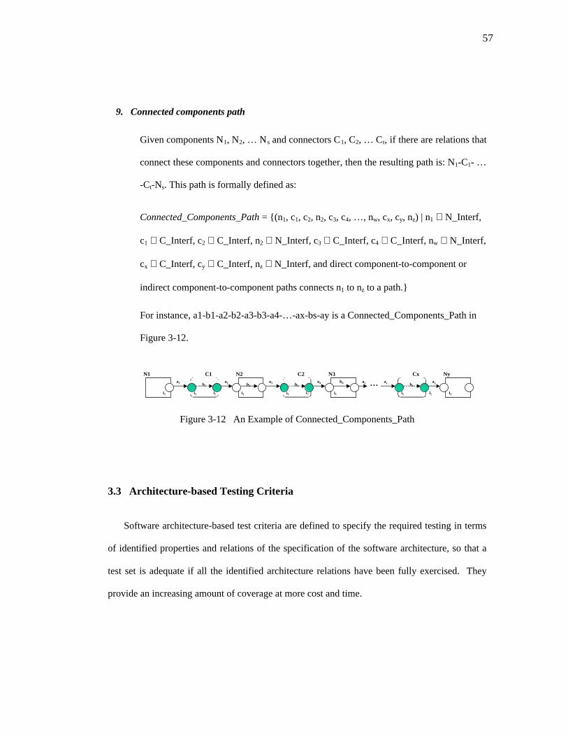
57
9. Connected components path
Given components N1, N2, … Ns and connectors C1, C2, … Ct, if there are relations that
connect these components and connectors together, then the resulting path is: N1-C1- …
-Ct-Ns. This path is formally defined as:
Connected_Components_Path = {(n1, c1, c2, n2, c3, c4, …, nw, cx, cy, nz) | n1 ∈ N_Interf,
c1 ∈ C_Interf, c2 ∈ C_Interf, n2 ∈ N_Interf, c3 ∈ C_Interf, c4 ∈ C_Interf, nw ∈ N_Interf,
cx ∈ C_Interf, cy ∈ C_Interf, nz ∈ N_Interf, and direct component-to-component or
indirect component-to-component paths connects n1 to nz to a path.}
For instance, a1-b1-a2-b2-a3-b3-a4-…-ax-bs-ay is a Connected_Components_Path in
Figure 3-12.
Figure 3-12 An Example of Connected_Components_Path
3.3 Architecture-based Testing Criteria
Software architecture-based test criteria are defined to specify the required testing in terms
of identified properties and relations of the specification of the software architecture, so that a
test set is adequate if all the identified architecture relations have been fully exercised. They
provide an increasing amount of coverage at more cost and time.
N1 C1a1 b1
i1 i1 i2
N2 C2a3 b3
i1 i1 i2
N3
i1
...Cx
ax bt
i1 i2
Ny
i1
b2a2 a4 a5 ayb4

58
1. Individual component interface coverage requires that the set of paths executed by the test
set T covers all Component_Internal_Transfer_Paths and
Component_Internal_Ordering_Rules for an individual component.
2. Individual connector interface coverage requires that the set of paths executed by the test
set T covers all Connector_Internal_Transfer_Paths and
Connector_Internal_Ordering_Rules for an individual connector.
3. All direct component-to-component coverage requires that the set of paths executed by the
test set T covers all C_N paths, all N_C paths and all Direct_Component_Paths.
4. All indirect component-to-component coverage requires that the set of paths executed by
the test set T covers all Indirect_Component_Paths.
5. All connected components coverage requires that the set of paths executed by the test set T
covers all possible Connected_Components_Paths for all the components in the
architecture.
Figure 3-13 shows how five different coverage levels are reflected in an example
architecture. Edges with specific numbers are the relations/paths that need to be tested for the
corresponding coverage levels. Path N1-C1-N2-C2-N3-C3-N4 is numbered with 5, this means
this path needs to be tested to satisfy coverage level 5 (All connected components coverage).
There are two level 4 paths (N1-C1-N2-C2-N3 and N2-C2-N3-C3-N4), three level 3 paths (N1-
C1-N2, N2-C2-N3, and N3-C3-N4), three level 2 paths (inside C1, C2, and C3), and three level
1 paths (inside N2, N3, and N4).

59
Figure 3-13 Coverage Levels
3.4 Architecture Coverage Analysis
Structural coverage analysis is needed to determine whether all architecture relations have
been covered. The architecture-based testing criteria defined in the previous section provide test
requirements that must be satisfied during testing. Test cases can then be generated specifically
to satisfy each test requirement or they can be generated separately and then checked to see if
they satisfy the requirements. In general, test coverage is measured by calculating the number of
internal arcs, external arcs and paths. A general way to measure test coverage is given as
follows.
Given a software architecture described by a certain ADL, we can construct its ICG. As
defined in the previous section, ICG = (N, C, N_Interf, C_Interf, N_Ex_arc, C_Ex_arc,
N_In_arc, C_In_arc), test coverage can be represented by ICG edge and node coverage. Let EA
be the number of external arcs in the ICG, IA be the number of internal arcs in the ICG, and
NInterf be the number of component and connector interfaces:
1. EA = | N_Ex_arc | + | C_Ex_arc |
N1 C13 2
N2 C2
3 213
N3
13
4
C3
2
N4
1
4
5
3 3

60
2. IA = | N_In_arc | + | C_In_arc |
3. NInterf = | N_Interf | + | C_Interf |
4. AINN = number of all indirect component-to-component paths
5. INi = number of internal relations inside a component Ni that have been tested
6. ICi = number of internal relations inside a connector Ci that have been tested
7. DNN = number of all direct component-to-component relations that have been tested
8. INN = number of all indirect component-to-component relations that have been
tested
9. AN = number of all connected components relations that have been tested
Then we have the following test coverage defined:
Individual component interface test coverage = INi / | Ni_In_arc |
Individual connector interface test coverage = ICi / | Ci_In_arc|
All direct component-to-component test coverage = DNN / (EA / 2)
All indirect component-to-component test coverage = INN / AINN
All connected components coverage = AN / | N_In_arc |
Test coverage analysis can be used to determine how much of the overall architecture has
been tested for given test case sets. This evaluation can be very helpful when we need to know
when to stop testing.
For instance, if we would like to check the individual connector interface (connector CS1)
test coverage in the ICG showed in Figure 3-3, if only one edge b1 has been covered in a test
set, while there are two internal arcs within that connector CS1, then individual connector CS1
interface coverage is ICi / | Ci_In_arc| = 1/2 = 50 %.

61
In conclusion, this chapter discusses a new testing technique at the software architecture
level. Architecture relations are the main focus of this technique, and they are formally defined.
The Interface Connectivity Graph (ICG) is introduced to help to represent the architecture
relations. Testing requirements and criteria are formally defined. Test coverage and analysis are
also formally defined in this chapter. This testing technique applies to general ADLs. Given a
specific ADL, we may have the capability to describe a software architecture with more details,
then we need to apply the architecture-based testing technique at a more detailed level as
presented in Chapter 4, in which a specific ADL Wright is used, and another graphical
representation is used.

62
Chapter 4 Testing Technique Applied to Wright
This chapter presents an application of the architecture-based testing technique to a specific
ADL, Wright. Because the software architecture-based testing technique presented in Chapter 3
is based on the ICG representation, to apply this technique to Wright, we need to develop a
mapping from a Wright description to an ICG (Interface Connectivity Graph). Also, as Wright
provides detail descriptions of interface behavior of components and connectors, we introduce
another type of graphical representation, the Behavior Graph (BG), based on the theory of Petri
Net [Peterson81, RT86]. Then we derive detailed test requirements (in terms of path coverage)
and testing sets based on the ICG and the BG. The application procedures are shown in Figure
4-1. The relation between an ICG and a BG is discussed, test data generation algorithms are
defined for automatic test requirements generation. Some issues related to this application are
also discussed at the end of the chapter.
Figure 4-1 Application Procedures
A Specific ADLDescription
Test Requirements(path coverage)
Test Sets forModeling or Testingthe ADL Description
The ICG
The BG
Part 2
Applying the Testing Technique to An ADL
Test Criteria (Defined in Chapter 3)
Implementation inChapter 6

63
4.1 ADL Wright in Brief
Architecture Description Languages (ADLs) are designed to provide ways to formally
describe software architectures. A large number of ADLs have been proposed [LV95, SDK+95,
Ves96, Tra93, MTW96, AG94a], each of which specifies a particular formal model in which
some aspects of a software architecture can be described. The formal architecture specifications
and descriptions allow us to algorithmically define test criteria and test sets. To apply the
software architecture testing technique described in Chapter 3, a specific ADL needs to be
chosen. There are three reasons we choose Wright as the basis for this application. First, Wright
explicitly defines components, connectors, and configurations of a software architecture, while
many other ADLs may not have explicit descriptions for connectors. Second, Wright is well
studied and there is a downloadable tool for Wright [Wrighttool]. Third, Wright has been
applied to several realistic application examples [AGI98, All97]. They provide valuable
resources for validation of the test criteria. Table 4-1 shows the Wright capability based on an
ADL survey [Med97].
Table 4-1 Representation Capability of Wright
Software Architecture Artifacts Wright
interface port
Component semantics computation and ports
interface role
semantics glueConnector
constraints role and glue
Configuration implicit or explicit? explicit

64
4.2 Mapping Wright to Interface Connectivity Graphs (ICG)
As described in Chapter 2, in a Wright description basic elements are components, which
are independent computational elements, and connectors, which define the interactions among
them. Wright components and connectors are instantiated and bound together in well-defined
ways to form configurations.
A component type consists of some number of ports (interfaces) and optionally, a
computation. Each port represents an interaction in which the component may participate and
describes expectations about how the component uses the port. The computation defines what
the component does and how the component uses the interactions described by the ports. A
Wright connector type consists of a set of roles and the glue. Each role in a connector defines
what is expected of any component that will participate as part of the interaction. The glue for a
connector describes how the roles work together to form an interaction. The components and
connectors of a Wright description are combined into a configuration to describe a complete
system architecture. Wright requires that each instance be explicitly and uniquely named. An
attachment defines the configuration by defining which component interfaces participate in
which connector roles.
An ICG only captures the structural relations in a Wright description, it visually contains all
the components and their interfaces (ports in Wright), all the connectors and their interfaces
(roles in Wright), and shows connections between component and connector interfaces and
possible connections inside components and connectors. But an ICG does not capture the
detailed behavioral information that some ADLs provide. To translate a Wright description to

65
an ICG, we need structural information such as component-port, connector-role relations and
configuration information from a Wright description.
An ICG can be represented by the structural properties of a Wright description. Each
Wright component corresponds to an ICG component box, ports of a Wright component
correspond to the interface circles in an ICG component box, and possible links among ports
described by the component computation are reflected as the component internal arcs inside an
ICG. Each Wright connector is represented by an ICG connector box, and the roles correspond
to the interface circles of the ICG connector box. Wright glue will link these circles in the ICG
connector box. A name mapping mechanism maps the instance names to their corresponding
component and connector names. An attachment decides the linkage between components and
connectors. The following shows a Wright description structure where components, connectors,
instances, and the attachment are described.
Wright Description Structure
Component C1
Port 1 [ describes how the component expects to interact in connection 1 ]
…..
Port n [ describes how the component expects to interact in connection n ]
Computation [ ties Port 1 … and Port n together ]Component C2
Port 1 [ describes how the component expects to interact in connection 1 ]
…..
Port m [ describes how the component expects to interact in connection m ]
Computation [ tie Port 1 … and Port m together ]Connector C1-C2 Connector
Role 1 [ describes what is expected of any component that will participate in interaction 1]
……
Role s [ describes what is expected of any component that will participate in interaction 1]
Glue [ describes how the participants work together to create an interaction]Instances
component1: C1
component2: C2
connect: C1-C2 Connector

66
Attachments:
component1 provides as C1-C2.C1
component provides as C1-C2.C2
end
Table 4-2 gives the structural mapping from a Wright description to an ICG. Wright
components and ports become the ICG components and interfaces, Wright connectors and
interfaces become the ICG connectors and corresponding interfaces. Component computations
provide the information for possible links among ports inside a component in an ICG. Wright
attachments provide links between component interfaces and their corresponding connector
interfaces.
Table 4-2 ICG Elements and Wright Elements
Wright Element (Instantiated) ICG ElementsComponents NConnectors CPorts of Components N_InterfPorts of Connectors C_InterfConnector Glue and Attachment N_Ex_arcConnector Glue and Attachment C_Ex_arcComponent Computation N_In_arcConnector Glue C_In_arc
4.3 Mapping Wright to Behavior Graph (BG)
In this section, we introduce a new graphical representation to describe the port and role
behaviors described in Wright. We discuss why we need the Behavior Graph (BG), how it is
defined, and how Wright descriptions are mapped into BGs.

67
4.3.1 ICG Is Not Enough -- Behavior Graph
An ICG provides a high level abstraction of a software architecture. But some ADLs
provide more detailed information about interface behavior and their relations or constraints.
Wright gives behavioral descriptions of component and connector ports and how they should
work together. In order to reflect this type of information in testing, we introduce a new type of
graphical representation, the Behavior Graph (BG), to represent the information about the port
behavior of two components and their connections. We found that Petri Net [Peterson81, RT86]
is a very good choice to describe the port or role behavior (as discussed below in section
4.3.1.1). We define the BG based on the Petri Net theory. An introduction to Petri Net theory
was given in Chapter 2.
4.3.1.1 Revised Petri Net (RPN)
Petri Nets are used to formally modeling distributed systems because Petri Nets provide
graph-theoretic representations of the communication and control patterns, and mathematical
frameworks for analysis and validation [Peterson81, Jin94]. Petri Net modeling is useful in this
application for several reasons. First, Petri Nets can capture the precedence relations and
structural interactions of concurrent and asynchronous events and can provide an integrated
methodology, with well-developed theoretical and analytical foundations. Second, the graphical
nature of Petri Nets allows the systems to be visualized. Third, the mathematical representations
of Petri Nets allow quantitative analysis to be used when generating test cases. Finally, Petri
Nets can be executed, allowing the dynamics of a system to be explored.

68
Formal definition for Petri Nets was given in Chapter 2. To suit our particular needs in the
context of software architecture, we need to introduce three changes to the Petri Nets. The
resulting graph is named a Revised Petri Net (RPN). Given a Petri Net N(P, T, I, O) as defined
in Chapter 2, a Revised Petri Net RPN(P, T, I, O) has three differences:
• Represent "the end of process". RPN.P now includes a new type of place pend that
represent the end of the process, a thick-lined place. This is just a notation change that does
not affect any theoretical properties of Petri Nets.
• Add "internal choice". RPN.I and RPN.O now include the representation of internal
choices Iinternal or Ointernal. Internal choices are non-deterministic choices made by the
process itself. Internal choices are presented by arcs that have small vertical lines, as shown
in Figure 4-2. This means when there is a token in p3, either transition t2 or t3 will fire.
The choice is made internally by the process itself. This is not only a notation representation
change, but also will affect the execution result.
Figure 4-2 Internal Choice Arcs
• Add "external choice". RPN.I and RPN.O now include the representation of external
choices Iexternal or O external. External choices are deterministic choices made by the
environment rather than by the process itself. In the context of Wright, it means that an
input arc comes from another component help to make the decision. Internal or external
p3
t2
t3

69
choices are presented by arcs that have double vertical lines, as shown in Figure 4-3. This
means when there is a token in p3, either transition t2 or t3 will fire, the choice is made
externally by input arcs from other components. This is a notation change, in the context of
software architecture, whenever there is an external choice, there is always another arc from
another component of the net to help enable the firing. Therefore, the choice is determined
by the availability of some resource from other components. This is the external choice
case.
Figure 4-3 External Choice Arcs
4.3.1.2 Behavior Graph (BG)
A Behavior Graph (BG) is an RPN that shows the behavior and the relation of two related
components. A BG consists of two component subnets, with each representing the behavior of
one component. A BG also has other places and transitions to show the connections of the two
components. Each component subnet contains one or more port subnets that describe the
expected behavior of each port. These ports may have transfer relations, ordering relations or
they may not have any relations at all. Transfer relations are described by place and transition
linkages from one port subnet to another, ordering relations are represented separately by a
computation subnet that describe the rules of ordering. Currently we consider the computation
p3
t2
t3
from another component

70
subnet a separate subnet inside a component subnet, it plays a role in generating test sets when
there are ordering relations among the ports. Each transition and place in a component subnet
will be named with the component's name as prefix. Formally, a BG is defined as follows:
Definition 4.1 Behavior Graph
Behavior Graph = (Comp1(Pn1, Tn1, In1, On1), Comp2(Pn2, Tn2, In2, On2), Pc, Tc, Ic, Oc), where
• Comp1 is the graph that describes component C1. Comp 1(Pn1, Tn1, In1, O n1) is a 5-tuple
representation of the graph. Pn1 is the set of all the places in C1, Tn1 is the set of all
transitions in Comp1, and In1 and On1 are the input and output arc sets.
• Comp2 is the graph that describes component C2. Comp2(Pn2, Tn2, In2, On2) is a 5-tuple
representation of the graph. Pn2 is the set of all the places in Comp2, Tn2 is the set
of all transitions in Comp2, and In2 and On2 are the input and output arc sets.
• Pc is a set of places that are used to connect components Comp1 and Comp2.
• Tc is a set of transitions that are used to connect components Comp1 and Comp2.
• Pn1 ∩ Pn2 ∩ Pc = ∅, Tn1 ∩ Tn2 ∩ Tc = ∅
• Ic is a set of arcs, each of which connects a place to a transition between two
components. Ic: ({Pn1, Pn2, Pc} × {Tn1, Tn2, Tc}) → {0,1}. If the value is 1, then the
arc exists, otherwise the arc does not exist.
• Oc is a set of arcs, each of which connects a transition to a place between two
components. Oc: ({Tn1, Tn2, Tc} × {Pn1, Pn2, Pc}) → {0,1}. If the value is 1, then
the arc exists, otherwise the arc does not exist.
When there is only one component, then the Behavior Graph becomes (Comp1(Pn1, Tn1,
In1, On1)).
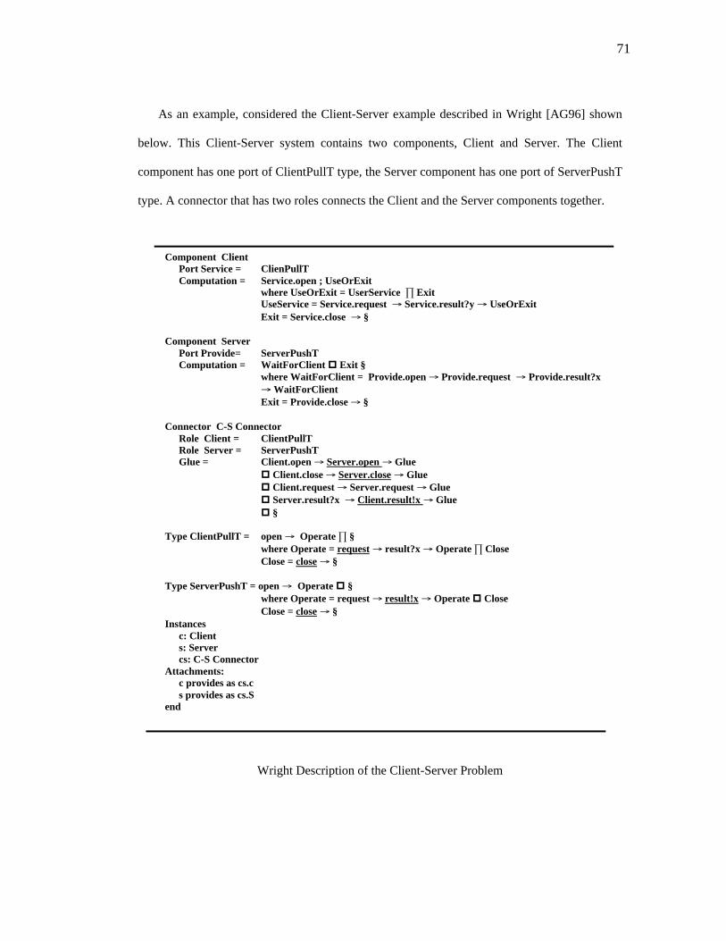
71
As an example, considered the Client-Server example described in Wright [AG96] shown
below. This Client-Server system contains two components, Client and Server. The Client
component has one port of ClientPullT type, the Server component has one port of ServerPushT
type. A connector that has two roles connects the Client and the Server components together.
Component ClientPort Service = ClienPullTComputation = Service.open ; UseOrExit
where UseOrExit = UserService Exit UseService = Service.request Service.result?y UseOrExit Exit = Service.close §
Component ServerPort Provide= ServerPushTComputation = WaitForClient Exit §
where WaitForClient = Provide.open Provide.request Provide.result?x WaitForClient Exit = Provide.close §
Connector C-S ConnectorRole Client = ClientPullTRole Server = ServerPushTGlue = Client.open Server.open Glue Client.close Server.close Glue
Client.request Server.request Glue Server.result?x Client.result!x Glue §
Type ClientPullT = open Operate § where Operate = request result?x Operate Close
Close = close §
Type ServerPushT = open Operate § where Operate = request result!x Operate Close
Close = close §Instances
c: Clients: Servercs: C-S Connector
Attachments:c provides as cs.c
s provides as cs.Send
Wright Description of the Client-Server Problem
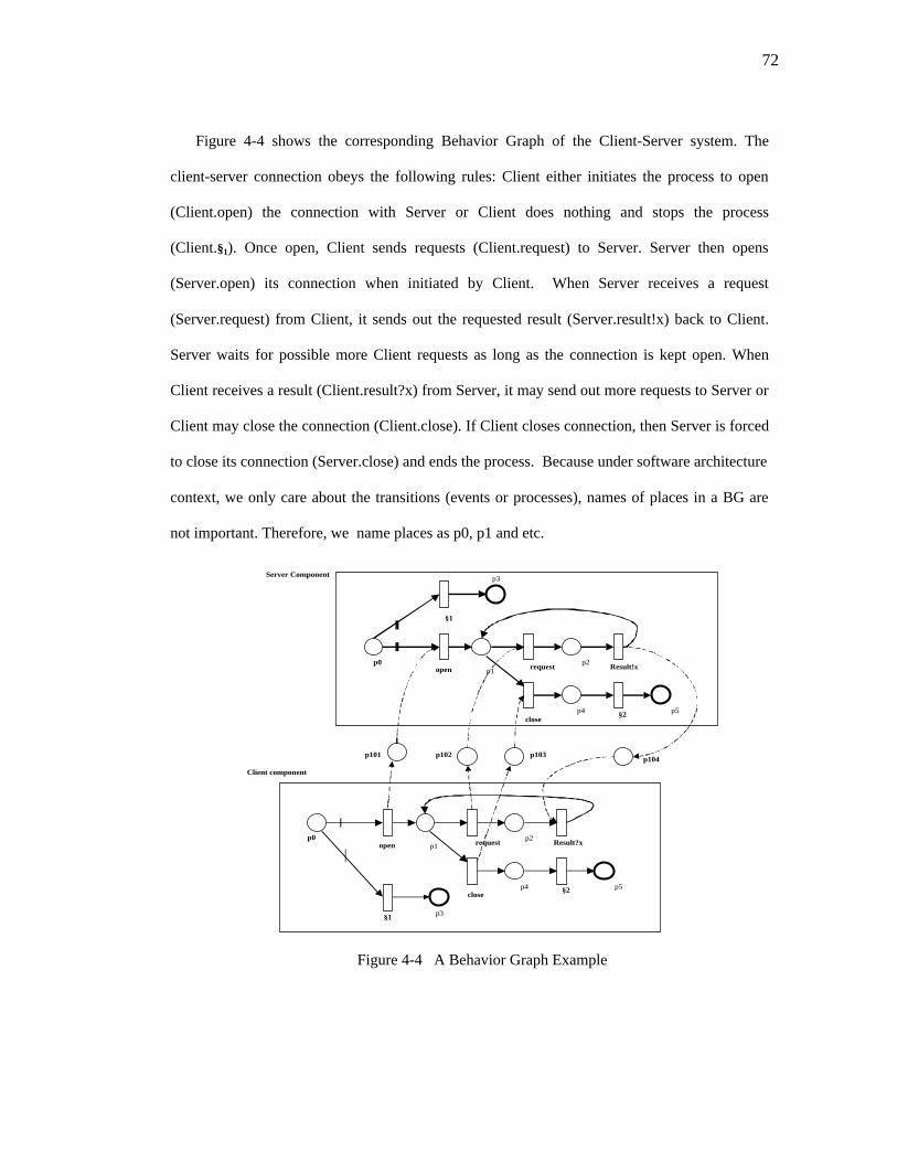
72
Figure 4-4 shows the corresponding Behavior Graph of the Client-Server system. The
client-server connection obeys the following rules: Client either initiates the process to open
(Client.open) the connection with Server or Client does nothing and stops the process
(Client.§1). Once open, Client sends requests (Client.request) to Server. Server then opens
(Server.open) its connection when initiated by Client. When Server receives a request
(Server.request) from Client, it sends out the requested result (Server.result!x) back to Client.
Server waits for possible more Client requests as long as the connection is kept open. When
Client receives a result (Client.result?x) from Server, it may send out more requests to Server or
Client may close the connection (Client.close). If Client closes connection, then Server is forced
to close its connection (Server.close) and ends the process. Because under software architecture
context, we only care about the transitions (events or processes), names of places in a BG are
not important. Therefore, we name places as p0, p1 and etc.
Figure 4-4 A Behavior Graph Example
Server Component
open request Result?xp1
p3
p2
p4 p5
§1
§2close
open request Result!x
close
p1
p3
p2
p4 p5
§1
§2
p0
p0
p101 p102 p103p104
Client component

73
The following shows the BG in the form of (Comp1(Pn1, Tn1, In1, On1), Comp2(Pn2, Tn2, In2,
On2), Pc, Tc, Ic, Oc). Note that for two transitions that have the same names in a subnet, we use
subscripts to differentiate them. For example, both Client and Server components have two §
transitions, we use §1 and §2 to differentiate the transitions.
Client = {P(client.p0, client.p1, client.p2, client.p3, client.p4, client.p5),
T(client.open, client.request, client.result?x, client.close, client.§1, cleint.§2),
I((client.p0, client.open), (client.p1, client.request), (client.p2, client.result?x),
(client.p1, client.close), (client.p0, client.§1,), (client.p4, client.§2)),
O((client.open, client.p1), (client.§1, client.p3), (client.request, client.p2),
(client.result?x, client.p1), (client.§2, client.p5), (client.close, client.p4)) }
Server = {P(server.p0, server.p1, server.p2, server.p3, server.p4)
T(server.open, server.request, server.result!x, server.close, server.§1,
server.§2),
I((server.p0, server.open), (server.p1, server.request), (server.p2, server.result!x),
(server.p1, server.close), (server.p4, server.§2), (server.p0, server.§1)),
O((server.open, server.p1), (server.request, server.p2), (server.result!x, server.p1),
(server.§1, server.p3), (server.close, server.p4), ), (server.§1, server.p5))}
Pn = {p101, p102, p103, p104}
Tn = {}
In = {(p101, server.open), (p102, server.request), (p103, client.close), (p104, client.result?x)}
On = {(clinet.open, p101), (client.request, p102), (server.result?x, p104),(Client.close, p103)}
It can be seen from this example that the behavior inside a component interface and across
two components can be represented statically and dynamically in terms of a BG representation,

74
marking, and firing sequences. Static information is represented in the BG structure, while the
dynamic features can be shown through the execution of the Revised Petri Nets. The BG will
further be used to help generate test cases under defined testing criteria.
Now we define some BG paths. These paths will be used in generating test requirements
and test cases.
Definition 4.2 BG Path
A BG path is a set of k place / transition nodes and k - 1 directed arcs, for some
integer k, such that the ith directed arc either connects the ith node to the (i+1)th node
or the (i + 1)th node to the ith node.
Definition 4.3 BG component behavior path (B-path)
A BG B-path is a BG path within a component interface subnet. It starts with the start
place of a component and ends with an end place. When there are loops in the subnet,
only one loop can be allowed in each behavior path. I.e., each node (place or
transition) is allowed to be visited at most twice in each B-path.
As an example, consider Figure 4-4. The behavior–paths in Client are:
1. client.p0-- client.open -- client.p1 -- client.request -- client.p2 -- client.result?x --client.p1 -- client.close -- client.p4 – client.§2 – client.p5
2. client.p0 -- client.§1-- client.p3
3. client.p0 -- client.open -- client.p1 -- client.close -- client.p4 -- client.§2 --client.p5
For instance, in behavior path 1 presented above, the path traversed back to client.p1
after transition client.result?x.

75
Definition 4.4 BG Component Connection Path (C-path)
A BG C-path is a BG path that crosses two component subnets A and B. It starts with
a place in component subnet A, where this place's output transition leads to the
connection of component subnet B. The path ends with the place in B that is the output
place of the transition that has a connection with A. In the context of software
architecture, connections between components in BGs are always from transitions
(events or processes) to transitions.
For example, all the BG C-paths from Figure 4-4 are shown as follows.
1. client.p0 -- client.open – p101 – server.open -- server.p1
2. client.p1 -- client.request – p102 – server.request – server.p2
3. server.p2 -- server.result!x – p104 -- client.result?x – client.p1
4. client.p1 -- client.close – p103 – server.close – server.p4
Definition 4.5 BG Interface Interaction Path (I-path)
A BG I-path is a BG path that crosses two component interface subnets A.I1 and A.I2.
The I-path starts with a place (circle) in component interface subnet A.I1, where this
place's output transition (rectangle) leads to the connection of another interface subnet
A.I2. The path ends with the place in A.I2 that is the output place of the transition that
has a connection with A.I1.
The example in Figure 4-5 shows a component with two ports, In and Out. There
are some connections between port In and port Out inside the component. I-paths show
the connections between ports inside the component.
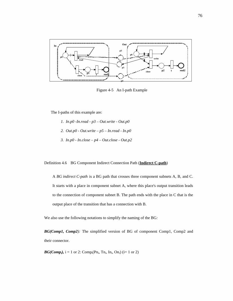
76
Figure 4-5 An I-path Example
The I-paths of this example are:
1. In.p0 -In.read - p3 – Out.write - Out.p0
2. Out.p0 - Out.write – p5 – In.read - In.p0
3. In.p0 - In.close – p4 – Out.close - Out.p2
Definition 4.6 BG Component Indirect Connection Path (Indirect C-path)
A BG indirect C-path is a BG path that crosses three component subnets A, B, and C.
It starts with a place in component subnet A, where this place's output transition leads
to the connection of component subnet B. The path ends with the place in C that is the
output place of the transition that has a connection with B.
We also use the following notations to simplify the naming of the BG:
BG(Comp1, Comp2): The simplified version of BG of component Comp1, Comp2 and
their connector.
BG(Compi), i = 1 or 2: Compi(Pni, Tni, Ini, Oni) (i= 1 or 2)
read
close §p1
In Out
write
close §p2
p3
p4
end1
end2p5
p0p0

77
C_Ex_arc(Comp1, Comp2): The Ex_arcs of component Comp1 to the connector that
connects to component Comp2.
N_Ex_arc(Comp1, Comp2): The Ex_arcs of connector that connects Comp1 and Comp2.
C_In_arc(Comp1): The internal arcs of component Comp1.
N_In_arc(Conn1): The internal arcs of connector Conn1.
BG Mathematical Representation
As with any other graphs, a Petri Net with n places and m transitions can be represented
by an n × m Incidence Matrix, C. The rows correspond to places and the columns
correspond to transitions. The cells are defined as follows:
• Cij = 1 if there is a directed arc from the j-th transition to the i-th place. "1"
indicates that the firing of the j-th transition adds one token to the i-th place.
• Cij = -1 if there is a directed arc from the i-th place to the j-th transition. "-1"
indicates that the firing of the j-th transition removes one token from the i-th place.
• Cij = 0 if there is no arc from the j-th transition to the i-th place.
• Cij = -0.5 if there is a directed arc from the i-th place to the j-th transition, and the
arc is an internal choice or an external arc.
The incidence matrix of the BG in Figure 4-4 is shown in Figure 4-6. To save space, we
prefix server with s and client with c. In this matrix transitions are grouped in two components.
Places are partitioned into 3 groups, two come from the two components, and the other group

78
contains places that connect the two component interfaces. In Figure 4-6, places s.p0 through
s.p5 is a group of places from component Server, c.p0 through c.p5 is a group of places from
component Client, and places p101 through p104 is group of places that connect Server and
Client.
s.open s.request s.result s.close s.§1 s.§2 c.open c.request c.result c.close c.§1 c.§2 s.p0 -0.5 0 0 0 -0.5 0 0 0 0 0 0 0s.p1 1 -0.5 1 -0.5 0 0 0 0 0 0 0 0s.p2 0 1 -1 0 0 0 0 0 0 0 0 0s.p3 0 0 0 0 1 0 0 0 0 0 0 0s.p4 0 0 0 1 0 -1 0 0 0 0 0 0s.p5 0 0 0 0 0 1 0 0 0 0 0 0
c.p0 0 0 0 0 0 0 -0.5 0 0 0 -0.5 0c.p1 0 0 0 0 0 0 1 -0.5 1 -0.5 0 0c.p2 0 0 0 0 0 0 0 1 -1 0 0 0c.p3 0 0 0 0 0 0 0 0 0 0 1 0c.p4 0 0 0 0 0 0 0 0 0 1 0 -1c.p5 0 0 0 0 0 0 0 0 0 0 0 1
p101 -1 0 0 0 0 0 1 0 0 0 0 0p102 0 -1 0 0 0 0 0 1 0 0 0 0p103 0 0 0 -1 0 0 0 0 0 1 0 0p104 0 0 1 0 0 0 0 0 -1 0 0 0
Figure 4-6 The Incidence Matrix of the Client-Server Example
4.3.2 Mapping Wright Descriptions to Behavior Graphs
To represent a Wright description with a BG is more complicated than to map a Wright
description to an ICG. As described in the above section, the behavior properties of a Wright
description can be viewed as three parts: the component (the actual behavior of a component),
the connector (the expected behavior of a component), and the connections of all the
components. Each component is represented by a component RPN subnet and each connector

79
can also be represented by a connector subnet. Because ports have to obey rules defined by
roles, we assume that they are identical here. So we do not produce repetitive role subnets.
4.3.2.1 Mapping Procedures
Figure 4-7 shows the mapping from a Wright description to a BG representation, where port
descriptions become the port subnets inside a component subnet. A component computation
provides information of possible transfer links among ports of the component; it also may form
a computation subnet if ordering rules are described in the computation. The glue of a connector
helps to form the transfer linkage between two components, and there will be a glue subnet if
there are ordering rules between connector roles.
Figure 4-7 Wright Description to BG Mapping
Component C1 Subnet
…...
port1 subnet
portn subnet
Component C2 Subnet
…...
port1 subnet
portm subnet
transferrelation
Component C1Computation subnet
Component C2Computation subnet
Connector C1-C2Glue subnet
ordering relation ordering relation ordering relation
transfer relationtransfer relation
Component C1 port1 …. portn
computation [……]
Component C2 port1 …. portm
computation [……]
Connector C1-C2
role 1role 2
Glue […… ]
Wright Description

80
Figure 4-8 shows the mapping relations and procedures. The mapping procedure is divided
into four parts: (1) map a port description to a BG subnet, (2) map a computation description to
a BG subnet, (3) map a glue description to a BG subnet, and (4) name mapping from a Wright
configuration and the attachment. A set of transformation rules needs to be defined and used in
the transformation process. As for the connector roles, we are assuming that a port behavior is
identical to the role it connects to, so no duplicate role subnet is produced in the process. Role
behaviors can be defined differently from the behaviors that they are connecting to. Port
behavior must obey what is defined in the connecting role. Petri Net analyses techniques such as
consistency checks, deadlock checks, and etc. [Peterson81] can be applied to check the subsume
relations between a role and a port. This is beyond the scope of this thesis.
Figure 4-8 Wright to ICG Transforming Procedures
Wright Description
Component Connector Configuration/Attachment
port1 …… portn computation role1 …… rolem glue instantiations of components and connectors
port1subnet
portn
subnet
computation subnet andports subnet linkage
assumed to bethe same as portsubnets
glue sunbet and component to Component subnets linkage
name mapping
transformation rules
map port tosubnetalgorithm
map computationto subnet algorithm
map glue tosubnet algorithm
name mapping table

81
In order to map a Wright description to a BG systematically, we need the syntax definition
of the ADL Wright. A full Backus-Naur Form (BNF) of Wright [Wrighttool] is given in
Appendix A. Now we present a way to map a subset of the ProcessExpression of the Wright
BNF form to Petri Net based on Goltz and Reisig's work [GR84]. They discussed transforming
a subset of the process algebra CSP (Communicating Sequential Processes) programs to Place
Transition Nets. Our mapping is based on their theory, but differs from their work in that we are
using Wright syntax which is slightly different from CSP. Details about Wright syntax can be
found in Allen's work [All97]. Also, we use Petri Nets instead of Place Transition Nets. The
transformation rules are defined in the following section.
4.3.2.2 Transformation Rules
To represent CSP like Wright ProcessExpression, we define the following types of
transformation rules for mapping a Wright description to a Revised Petri Net (RPN, defined in
section 4.3.1).
Rule 1. Events e are translated as Transf[e]:
Rule 2. Events e?x are translated as Transf[e?x]:
Rule 3. Events e!x are translated as Transf[e!x]:
e
e?x
e!x

82
Rule 4. Process definitions P = e → P are translated as Transf[P = e → P] :
Rule 5. Event § is translated as Transf[§]:
Preset and Postset
Given a Petri Net (P, T, I, O), let x ∈ P ∪ T, the preset *x and postset x* is defined as
preset: *x = { y ∈ P∪ T | (y, x) ∈ ((P ×T)) ∪ (T × P)) }
postset: x* = { y ∈ P∪ T | (x, y) ∈ ((P × T)) ∪ (T × P)) }
The preset of a place x is a set of all transitions that have directed arcs pointed to the place
x. The postset of a place x is the set of all transitions that have directed arcs pointed from the
place x. The presets and postsets of transitions are defined in a complementary manner. The
concepts of preset and postset are very useful when combining subnets together.
For example, in Figure 4-9, *t1 = {p1}, t1* = {p2}, *t2 = {p2}, t2* = {p3}, *p1 = Ø, p1*
= {t1}, *p2 = {t1}, p2* = {t2, t3}, *p3 = {t2}, p3* = Ø, *p4= {t3}, p4* = Ø
Figure 4-9 The Preset/Postset Example
eP
§ end
t1p1 p2t2
t3
p3
p4

83
Definition 4.7 Sequential Net
An RPN net is sequential if and only if for all transitions ti ∈ T, |*ti| =|ti*| = 1. In RPN, we
extend the notion of sequential net such that |*ti| =|ti*| = 1 when ti is connected to two or
more internal choice arcs because only one of the choices will be taken. For instance, in
Figure 4-10, net A is a sequential net, net B is not a sequential net.
Figure 4-10 Sequential Net and Non-sequential Net
Now we define a sequential composition of two sequential RPN nets.
Definition 4.8 End Elements of a Net N•
The end elements of a RPN net is the set of all the elements (places or transitions) that have
only input arcs but no output arcs, or a designated one if the end element of the net is in a
loop.
N•(P, T, I, O) = {x ∈ P ∪ T | x* = ∅}
N• is the set of all the end elements (places or transitions) of a net.
t1p1 p2t2
t3
p3
p4
Net A
t1p1 p2t2
t3
p3
p4
Net B

84
Definition 4.9 Start Elements of a Net •N
The start elements of a RPN net is the set of all elements (places or transitions) that have
only output arcs but no input arcs, or a designated element if the start element of the net is
in a loop.
•N(P, T, I, O) = {x ∈ P ∪ T | *x = ∅}
•N is the set of all the start elements (places or transitions) of a net.
For example, Figure 4-11 shows a sequential net A and a non-sequential net B. C is a
sequential net with a loop. The start element set for A is {p1}, and the end element set for A is
{p4, p5}. C is also a sequential net, because the output arcs from e are internal choice arcs, only
one of them can be chosen at a time.
Figure 4-11 Sequential Net, Start/End Elements
Rule 6. Sequential Composition
This sequential composition operation combines two sequential Wright nets by obtaining
the end elements of the first net and the start elements of the second net and then linking
p1
t1
t2
t3
t4
p2
p3
p4
p5
t1
p2
p3p1
net A net B
ep1p2
net C
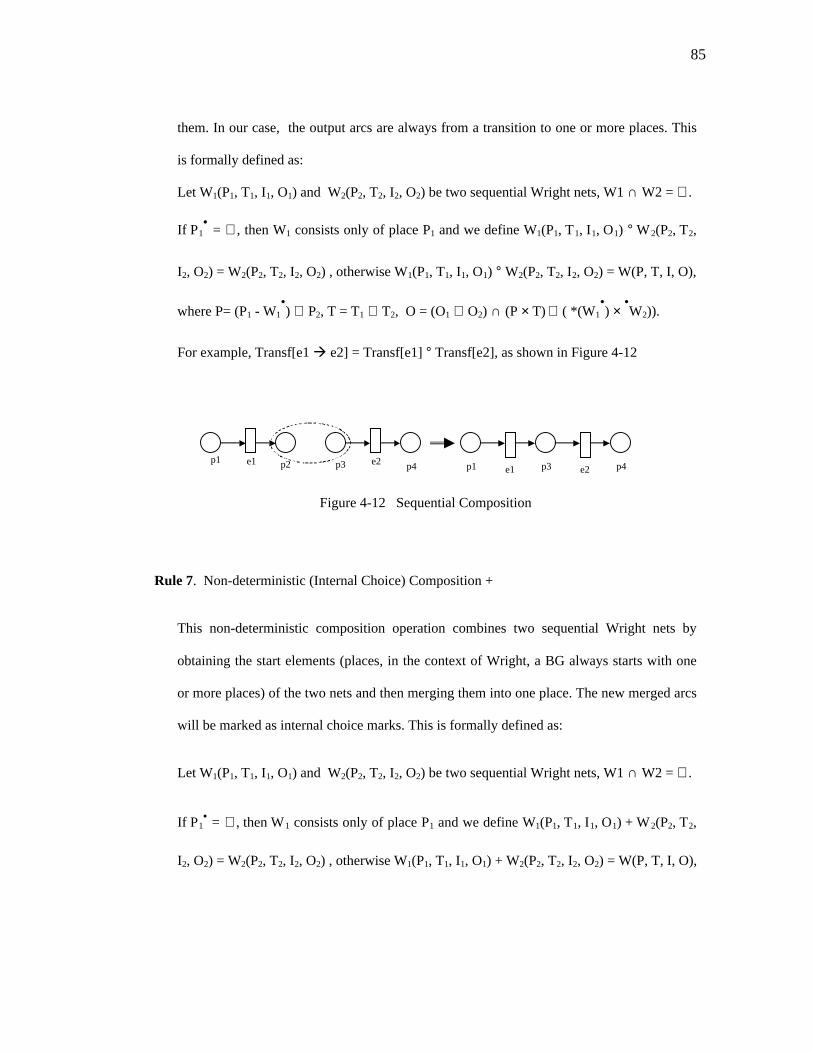
85
them. In our case, the output arcs are always from a transition to one or more places. This
is formally defined as:
Let W1(P1, T1, I1, O1) and W2(P2, T2, I2, O2) be two sequential Wright nets, W1 ∩ W2 = ∅.
If P1• = ∅, then W1 consists only of place P1 and we define W1(P1, T1, I1, O1) ° W2(P2, T2,
I2, O2) = W2(P2, T2, I2, O2) , otherwise W1(P1, T1, I1, O1) ° W2(P2, T2, I2, O2) = W(P, T, I, O),
where P= (P1 - W1•) ∪ P2, T = T1 ∪ T2, O = (O1 ∪ O2) ∩ (P × T) ∪ ( *(W1
•) ×
•W2)).
For example, Transf[e1 à e2] = Transf[e1] ° Transf[e2], as shown in Figure 4-12
Figure 4-12 Sequential Composition
Rule 7. Non-deterministic (Internal Choice) Composition +
This non-deterministic composition operation combines two sequential Wright nets by
obtaining the start elements (places, in the context of Wright, a BG always starts with one
or more places) of the two nets and then merging them into one place. The new merged arcs
will be marked as internal choice marks. This is formally defined as:
Let W1(P1, T1, I1, O1) and W2(P2, T2, I2, O2) be two sequential Wright nets, W1 ∩ W2 = ∅.
If P1• = ∅, then W1 consists only of place P1 and we define W1(P1, T1, I1, O1) + W2(P2, T2,
I2, O2) = W2(P2, T2, I2, O2) , otherwise W1(P1, T1, I1, O1) + W2(P2, T2, I2, O2) = W(P, T, I, O),
e1 e2e1 e2p1 p2 p3 p4 p1 p3 p4

86
where P= (P1 - (•W1 ∪
•W2) ∪ {p0}), T = T1 ∪ T2, I = ((I1 ∪ I2) - (
•W1 × ((
•W1)*) ∪ (•W2 ×
(•W2)*) ∪ ({p0} × (
•W1)*) ∪ ( {p0} × (
•W2)*)), O = (O1 ∪ O2) – (*(
•W1) ×
•W1 ) ∪
(*(•W1) × {p0}) ∪ (*(
•W2) × {p0}) ∪ (*(
•W2) ×
•W2))).
For example, Transf[P1 P2] = Transf[P1] + Transf[P2], where P1 = e2 → e2, P2 = e → P2.
This is shown in Figure 4-13.
Figure 4-13 Non-deterministic (Internal Choice) Composition
The only difference between the deterministic and the non-deterministic composition is that
the two choice arcs are different. The deterministic composition generates external choice arcs,
while the non-deterministic composition generates internal choice arcs.
Rule 8. Deterministic (External Choice) Composition ♦
This deterministic composition operation combines two sequential Wright nets by obtaining
the start elements (places) of the two nets and then merging them into one place. The new
merged arcs will be marked as external choice mark. The actual decision factor will be from
the interaction of another component. Details are discussed in the next section. This is
formally defined as:
e1 e2
eP
e1 e2
e

87
Let W1(P1, T1, I1, O1) and W2(P2, T2, I2, O2) be two sequential Wright nets, W1 ∩ W2 = ∅.
If P1• = ∅, then W1 consists only of place P1 and we define W1(P1, T1, I1, O1) ♦ W2(P2, T2,
I2, O2) = W2(P2, T2, I2, O2) , otherwise W1(P1, T1, I1, O1) ♦ W2(P2, T2, I2, O2) = W(P, T, I,
O), where P= (P1 - (•W1 ∪
•W2) ∪ {p0}), T = T1 ∪ T2, I = ((I1 ∪ I2) - (
•W1 × ((
•W1)*) ∪
(•W2 × (
•W2)* ) ∪ ({p0} × (
•W1)*) ∪ ( {p0} × (
•W2)*)), O = (O1 ∪ O2) – (*(
•W1 ) ×
•W1) ∪
(*(•W1) × {p0}) ∪ (*(
•W2) × {p0}) ∪ (*(
•W2) ×
•W2))). These replacement arcs are external
choice arcs.
For example, Transf[P1 ∏ P2] = Transf[P1] ♦ Transf[P2], here P1 = e2 → e2, P2 = e → P2.
This is shown in Figure 4-14.
Figure 4-14 Deterministic (External Choice) Composition
Rule 9. Parallel Composition ∪
The parallel composition operation combines two sequential Wright nets without
changing either one of them. The availability of tokens to initiate both sequential nets will
e1 e2
eP
e1 e2
e
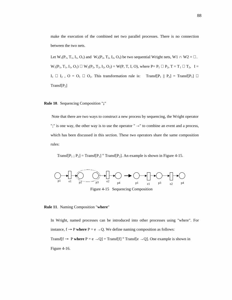
88
make the execution of the combined net two parallel processes. There is no connection
between the two nets.
Let W1(P1, T1, I1, O1) and W2(P2, T2, I2, O2) be two sequential Wright nets, W1 ∩ W2 = ∅.
W1(P1, T1, I1, O1) ∪ W2(P2, T2, I2, O2) = W(P, T, I, O), where P= P1 ∪ P2, T = T1 ∪ T2, I =
I1 ∪ I2 , O = O1 ∪ O2. This transformation rule is: Transf[P1 || P2] = Transf[P1] ∪
Transf[P2]
Rule 10. Sequencing Composition ";"
Note that there are two ways to construct a new process by sequencing, the Wright operator
";" is one way, the other way is to use the operator " " to combine an event and a process,
which has been discussed in this section. These two operators share the same composition
rules:
Transf[P1 ; P2] = Transf[P1] ° Transf[P2]. An example is shown in Figure 4-15.
Figure 4-15 Sequencing Composition
Rule 11. Naming Composition "where"
In Wright, named processes can be introduced into other processes using "where". For
instance, f P where P = e →Q. We define naming composition as follows:
Transf[f P where P = e →Q] = Transf[f] ° Transf[e →Q]. One example is shown in
Figure 4-16.
e1 e2e1 e2p1 p2 p3 p4 p1 p3 p4
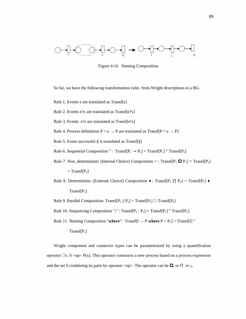
89
Figure 4-16 Naming Composition.
So far, we have the following transformation rules from Wright descriptions to a BG.
Rule 1. Events e are translated as Transf[e]
Rule 2. Events e?x are translated as Transf[e?x]
Rule 3. Events e!x are translated as Transf[e!x]
Rule 4. Process definitions P = e → P are translated as Transf[P = e → P]
Rule 5. Event successful § is translated as Transf[§]
Rule 6. Sequential Composition ° : Transf[P1 P2] = Transf[P1] ° Transf[P2]
Rule 7. Non_deterministic (Internal Choice) Composition + : Transf[P1 P2] = Transf[P1]
+ Transf[P2]
Rule 8. Deterministic (External Choice) Composition ♦: Transf[P1 ∏ P2] = Transf[P1] ♦
Transf[P2]
Rule 9. Parallel Composition: Transf[P1 || P2] = Transf[P1] ∪ Transf[P2]
Rule 10. Sequencing Composition ";" : Transf[P1 ; P2] = Transf[P1] ° Transf[P2]
Rule 11. Naming Composition "where": Transf[f → P where P = P1] = Transf[f] °
Transf[P1]
Wright component and connector types can be parameterized by using a quantification
operator ∀x: S <op> P(x). This operator constructs a new process based on a process expression
and the set S combining its parts by operator <op>. The operator can be p, or Π or ;.
f ef e Q Q

90
For instance, ∀x: {1, 2, 3} p Pi = P1 p P2 p P3
∀x: {1, 2, 3} Π Pi = P1 Π P2 Π P3
∀x: {1, 2, 3} ; Pi = (P1; P2; P3)Π (P1; P3; P2)
Π(P2; P3; P1)Π (P2 ; P1; P3)
Π(P3; P2; P1)Π (P3; P1; P2)
These types of parameterization normally occur in the component computation or connector
glue descriptions. They represent the possible transfer and ordering relations between
component ports. We translate them into RPN based on the following rules:
Rule 12. Transf[∀x: S p P(x)] = Transf[P(x1)] + Transf[P(x2)] + … + Transf[P(xn)]
In terms of RPN representation, we can put a place set S in the start place of the subnet that
represents all the available tokens (elements in S) that will participate in the subnet. This
shows in Figure 4-17. Firing of the transition P can be controlled as one at a time or allow
multiple firing at the same time.
Figure 4-17 Quantification Operator (1)
Rule 13. Transf[∀x: S Π P(x)] = Transf[P(x1)] ♦ Transf[P(x2)] ♦ … ♦ Transf[P(xn)].
In terms of RPN representation, we put a place set S in the start place in the subnet, its out
put arc is a external choice arc. This shows in Figure 4-18. Firing of the transition P can be
controlled as one at a time or allow multiple firing at the same time.
p
S
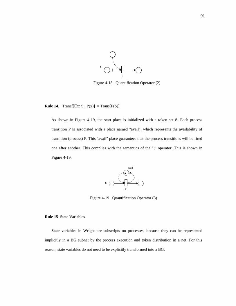
91
Figure 4-18 Quantification Operator (2)
Rule 14. Transf[∀x: S ; P(x)] = Trans[P(S)]
As shown in Figure 4-19, the start place is initialized with a token set S. Each process
transition P is associated with a place named "avail", which represents the availability of
transition (process) P. This "avail" place guarantees that the process transitions will be fired
one after another. This complies with the semantics of the ";" operator. This is shown in
Figure 4-19.
Figure 4-19 Quantification Operator (3)
Rule 15. State Variables
State variables in Wright are subscripts on processes, because they can be represented
implicitly in a BG subnet by the process execution and token distribution in a net. For this
reason, state variables do not need to be explicitly transformed into a BG.
p
S
p
avail
S

92
For example, from a Wright case study [All97], a component computation with state
variables is defined as follows:
Component Server (numclients: 1 ..) =
Port Client1..numClients = ServerPushTComputation = WaitForClient{},{}
where WaitForCliento,c = x: ((1..numClients) \ (O C)) Clientx.open DecideNextActionO {x}, C
DecideNextActionO,C = WaitForClientO,C x: O ReadFromClientx,O,C
O {} O C {1..numClients)DecideNextActionO,C = x: O ReadFromClientx,O,C
O {} O C = {1..numClients)DecideNextActionO,C = WaitForClient{},C
O = {} C {1..numClients)DecideNextAction{},{1..numClients} = §ReadFromClientx,O,C = Clientx.request Clientx.result!y DecideNextActionO,C
Clientx.close DecideNextAction O \{x}, C {x}
A State Variable Example
There are two state variables O and C. O indicates the number of clients that have been
opened and C indicates the number of clients that have closed their connections.
Combinations of four possible O and C states result in different processing steps. The
Wright computation description can be described by a Colored Petri Net [Jensen97] as
shown in Figure 4-20. The token distribution and execution of the net would show the same
behavior as described by the state variables in its Wright description.

93
Figure 4-20 Representation of Wright Computation
Rule 16. Constraints
Wright uses constraints as style restrictions. As our testing technique dose not focus on the
style constraints of a specific software architecture, we will not include mapping of Wright
constraints into BG. How to test whether a given architecture fits for a specific architecture
style is out of the scope of our research, however it remains a future research topic.
4.3.2.3 Completeness Discussion
We have defined 16 rules in the previous section to transform a Wright specification to a
Revised Petri Net. Events (e?x, e!x, §) and 6 operators ( →, p, Π , ||, ;, where, Π ) have had
transformation rules defined for them. The Universal quantifier ∀x: S p P(x) , ∀x: S Π P(x),
and ∀x: S ; P(x) have also had transformation rules defined for them. Process of state variables
is also discussed in brief (a more sophisticated form of Petri Net needs to be used in dealing
C.open
(1..numClients)o o o o
o
o
c
n’c
n’c
WaitDecide
client x
§
C.lose
C.requestC.result

94
with state variables). These cover all the operators defined in the Wright BNF
ProcessExpression as shown in Appendix A. Only style constraints are not discussed because
it is not in the scope of this dissertation.
4.3.2.4 An Example
The Read-Write model contains two components, component1 and component2.
Component1 has two ports, port In reads data from an other source, and port Out writes the
data that was just read from port In. Out also sends the data that was read to component2 port
In.
Component C1Port In = read?x In close §Port Out = write!x Out Close §Computation = (In.read?x Out.write!x Computation)
(In.close Out.close §)Component C2
Port In = read?x In close §Computation
Connector CCRole Input = read?x Input close § fail §Role Output = write!x Out Close §Glue = C1.write!x C2. read?x Glue close §
Instancescomponent1: C1component2: C2connect: C1-C2 Connector
Attachments:component1 provides as C1-C2.C1
component provides as C1-C2.C2end
The Read-Write Example
Figure 4-21 shows the BG representation of Component C1, C2, and their Connector CC.
The subnet of port Out should obey the rules of connector role Input, that is, the port subnet
should be a refinement of the role subnet. The computation of component C1 is shown as the

95
links between the two port subnets in component C1. The glue of the connector is shown as the
links between the component C1 and component C2 subnets.
Figure 4-21 A Wright to BG Example
4.4 ICG and BG Relations
For a given architecture Wright description, an ICG describes an architecture at a higher
level of abstraction than a BG does. An ICG hides behavioral details of component and
connector interfaces, while a BG represents the aggregated effect of the behaviors that are
modeled by the Revised Petri Net. As shown in Figure 4-22, a component or a connector
interface can be seen as a folded Petri Net (a Petri Net whose transitions and places can be
Component C1
read
close §p1
In
Outwrite
close §p2
p3
p4
Component C2
Inread
close§p2
ports
Computation ofa component
Glue
end1end2
end
p101 p102

96
decomposed into more Petri Nets), unfolding it reveals the details of the ports behavior. When
generating test cases, we can choose to either go to a higher level of abstraction or use more
detailed information about the components and connectors.
Figure 4-22 ICG and BG Relation
component1
port1
start end
open close
ICG Representation
p1 p2 p3 p4
p5
p6
component2
port1
start end
open close
p0
p1
p4
p2
p3
Component2
Component1
connector
role1 role2 role1 role2
BG Representation

97
When a BG contains a computation subnet that constrains the possible ordering information
among interfaces other than transfer relations, then the computation subnet provides the process
ordering guidance among the interfaces.
It can be seen that ICG arcs will be expanded in the corresponding BG representation. The
following table shows how ICG arcs expand in a BG representation.
Table 4-3 ICG and BG Relations
ICG Arcs BG Paths
C_Ex_arc(Comp1, Comp2) all the c_paths in the BG(Comp1, Comp2) from the initiation
component to the called component.
N_Ex_arc(Comp1, Comp2) all the c_paths in the BG(Comp1, Comp2) from the called
component to the initiation component.
C_In_arc(Comp1) all the I_paths between the two or more interface subnets in the
Comp1 subnet of the BG(Comp1, Comp2).
N_In_arc(Conn1) not explicitly represented in BG, each role is assumed to be of the
same behavior as its corresponding component port.
From Table 4-3, we can see that one ICG arc can sometimes be represented by multiple BG
paths based on the behavioral nature of the component ports. Therefore, as it comes to test
criteria coverage, we will apply the testing criteria on the ICG level and expand them to the BG
level.
4.5 Generating Test Requirements and Test Cases
With the ICG and the BG of a Wright architecture description available from the previous
sections, the testing criteria described in Chapter 3 can be applied to these two graphs. First we

98
look at how the testing relations described in Chapter 3 can be represented in terms of ICGs and
BGs. Table 4-4 gives the testing relations and their corresponding ICG or BG paths.
Table 4-4 Wright and ICG Mapping
# Testing Relations ICG or BG paths
1 Component_Internal_Transfer_Relation(N.interf1, N.interf2) BG I-paths
2 Component_Internal_Ordering_Relation(N.interf1, N.interface2) BG I-paths and ordering rules
3 Component_Internal_Relation(N1.interf1, N1.interf2) all BG I-paths from 1, 2 andordering rules
4 Connector_Internal_Transfer_Relation(C.interf1, C.interf2) BG I-paths
5 Connector_Internal_Odering_Relation(C.interf1, C.interface2) BG I-paths and ordering rules
6 Connector_Internal_Relation(C.interf1, C.interf2) all BG I-paths from 3,4 andordering rules
7 N_C_Relation(N.interf1, C.interf1) ICG paths and BG C-paths
8 C_N_Relation(C.interf1, N.interface1) ICG paths and BG C-paths
9 Direct_Component_Relation(N1.interf1, C1.interf1, C1.interf2,N2.interf2)
ICG paths and BG C-paths
10 Indirect_Component_Relation(N1.interf1, C1.interf1, C1.interf2,N2.interf2, C2.interf1, C2.interf2, N3.interf2)
ICG paths and BG C-paths
4.5.1 Applying Testing Criteria to Generate Testing Requirements
This section shows what testing requirements can be generated when applying the six
testing criteria defined in Chapter 3:

99
1. Individual component interface coverage requires that the set of paths executed by the test
set T covers all Component_Internal_Transfer_paths and
Component_Internal_Ordering_rules for an individual component.
This criterion generates these testing requirements: All the BG component subnet I-paths of
a particular component should be covered by the test set T, and ordering rules should be
applied to the corresponding component interfaces.
2. Individual connector interface coverage requires that the set of paths executed by the test
set T covers all Connector_Internal_Transfer_paths and Connector_Internal_Ordering_rules
for an individual connector.
This criterion generates these testing requirements: All the BG connector subset I-paths of a
particular connector should be covered by the test set T, and ordering rules should be
applied to the connector interfaces. This dissertation assumes that port behaviors are
considered to be the same as defined connector behaviors, so the testing requirements are
not tested explicitly.
3. All direct component-to-component coverage requires that the set of paths executed by the
test set T covers all C_N paths, all N_C paths and all Direct_Component_paths.
This criterion generates these testing requirements: All the BG C-paths between two related
components should be covered for those components that have direct component-to-
component relations.
4. All indirect component-to-component coverage requires that the set of paths executed by
the test set T covers all Indirect_Component_paths.

100
This criterion generates these testing requirements: All the BG C-paths and I_paths among
three related components should be covered, and all the ordering rules for those
corresponding interfaces should be applied.
5. All connected components coverage requires that the set of paths executed by the test set T
covers all Connected_Components_paths for all the components in the architecture.
This generates these testing requirements: All the BG component subnet I-paths for all the
components in the described system should be covered by the test set T, and ordering rules
should be applied to the corresponding component interfaces.
4.5.2 Test Case Generation Algorithms
Given a software architecture described in Wright, we can obtain its ICG and BG incidence
matrices as described in Chapter 3. The high level algorithm flow charts are represented in
Figure 4-23 through Figure 4-26. Algorithm details are presented in Chapter 5. Because test
case for criterion 5 can actually be generated from lower level criteria, the algorithm flow chart
for criterion 5 is not given here.

101
Figure 4-23 Test Set Generation 1
Figure 4-24 Test Case Generation 2.
BG port2BG port1
BG I-paths + B-paths +ordering rules
Test sequences
Component1
BG port2BG port1
Test sequences
Component2
BG port2BG port1
Test sequences
Componentn
Test Criterion 1 -- Individual Component Interface Coverage
BG I-paths + B-paths +ordering rules
BG I-paths + B-paths +ordering rules
BG role2BG role1
BG C-path + B-paths + ordering rules
Test sequences
Connector1
BG role2BG role1
Test sequences
Connector1
BG role2BG role1
Test sequences
Connectorm
Test Criterion 2 -- Individual Connector Coverage
BG C-path + B-paths + ordering rules
BG C-path + B-paths + ordering rules

102
Figure 4-25 Test Case Generation 3
Figure 4-26 Test Case Generation 4
BG port2
BG role2BG role1
BG port1BG port1BG port2
BG I-paths + ordering rules
Test sequences
BG I-paths + ordering rules
Test sequences
Component1 Component2
BG C-path + ordering rules
Test sequences
Connector1
Test Criterion 3 -- All Direct Component-to-Component Coverage
BG port2
BG role2BG role1
BG port1
BG role1
BG port1BG port1
BG port2BG port2
BG role2
BG I-paths + ordering rules
Test sequences
BG I-paths + ordering rules
Test sequences
BG I-paths + ordering rules
Test sequences
Component1 Component2 Component3
BG C-paths + ordering rules
Test sequences
BG C-paths + ordering rules
Test sequences
BG Indirect C-paths + ordering rules
Test sequences
Test Criterion 4 -- All indirect Component-to-Component Coverage
Connector1 Connector2

103
4.5.3 Test Procedure and Test Cases
As an example, one testing criterion is applied to the above Wright Client-Server example.
The Behavior Graph is shown in Figure 4-4. We present test scenarios three pieces of
information: (1) a time axis, (2) a list of components related to the test, in this example, the
Client and Server components, and (3) actions underlined with dashed lines indicating at which
time ti occurs. There are two different meanings for actions between two dashed lines: for those
actions between two dashed lines for the same component, it means a sequential action; for
those actions between two dash lines that are from different components, it means that the
actions can be taken with no specific sequence, that is, they can occur in parallel. If we choose
the testing criteria of "test all the component-to-component coverage", then we will have three
test cases.
Test Case 1. The first action is taken from the start of the time axis, t1, Client.open. If
Client is not waiting for any response from Server, then client.request results. In the mean time,
we expect the server side to open. The server.open action occurs independently of the
client.request result action. The server.request and server.result!x must happen sequentially after
time t2. Client will receive result in the next time period between t3 and t4, and may then
request for more results. Once Client sends its request, Server will receive the request and send
the result, then Client receives the result and closes up the connection, Finally, Server is
expected to close its connection when it knows Client has closed its connection.

104
Client Server
t1 open
opent2 result?x
request
t3 result!x
result?x
t4 requestrequest
t5 result!x
result?x
t6 close
t7 close
Test Case 2. Client opens the connection and requests result, in the mean time Server
opens the connection and receives request and then sends out results. Once Client receives
results, it closes the connection. Server then closes its connection.
Client Server
t1 open
open
t2 result?x request
t3 result!x
result?x
t5 close
t6 close
Test Case 3. Right after Client opens the connection, and when Server also connects, Client
closes up the connection, Server will then close the connection.
time(increase)
time(increase)
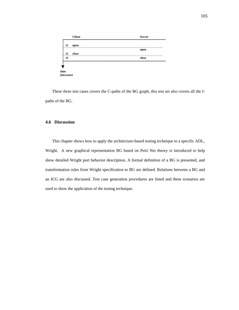
105
Client Server
t1 open
opent2 close
t3 close
These three test cases covers the C-paths of the BG graph, this test set also covers all the I-
paths of the BG.
4.6 Discussion
This chapter shows how to apply the architecture-based testing technique to a specific ADL,
Wright. A new graphical representation BG based on Petri Net theory is introduced to help
show detailed Wright port behavior description. A formal definition of a BG is presented, and
transformation rules from Wright specification to BG are defined. Relations between a BG and
an ICG are also discussed. Test case generation procedures are listed and three scenarios are
used to show the application of the testing technique.
time(increase)

106
Chapter 5 Prototype Tool
In order to demonstrate the effectiveness of the software architecture-based testing
technique, a prototype system was developed. This helps us to evaluate the technique and
examine its usefulness in generating test cases for an architecture description written in the
ADL Wright. This chapter describes the design and implementation of the prototype system
ABaTT (Architecture-Based Testing Tool) based on the software architecture-based testing
technique.
5.1 System Description
ABaTT is the prototype tool that was developed under Power Macintosh G3. It was written
in Java 1.2. The system was developed to meet two major objectives:
1) To implement and demonstrate the feasibility and effectiveness of the software
architecture-based testing technique
2) To generate test requirements (in terms of test paths) or to check test coverage on a
given test set
A high-level architecture structure is shown in Figure 5-1. The prototype tool takes a parsed
Wright architecture description. It generates the ICG and the BG incidence matrices. The
mapping between a Wright description and ICG and BG graphs was discussed in chapter 4.
The prototype tool test generation algorithm then generates tests to satisfy a given test criterion.

107
Figure 5-1 The Prototype Tool ABaTT
5.2 Assumptions and Design Structure
We made the following assumptions to the ABaTT tool. First, we assume that the input to
ABaTT is parsed Wright specifications in the form of binary trees, associated with tables that
describe the configurations information of the Wright specification. The binary trees describe
the ports and computations of components. Figure 5-2 shows a binary tree example, where a
Wright port description is given in the form of text, each node in the binary tree contains the
information of LeftChild, RightChild, NodeValue (String type), Visited, and BackLink (used
when there is a link back to a node). Glues and configuration information are stored in the tables
to record name mapping and port to port connection relations. To form the binary tree, we need
to build individual tree nodes by assigning the corresponding node names. For instance, we can
build a WrightTree node by instantiating a WrighTree object:
ICG Matrix
ArchitectureDescription by anADL (Wright)
Parse Wright
BG Converter
ICG Converter
BG Matrices
Test CaseGenerationAlgorithm
Test CoverageAnalysis
Algorithm
Test Cases
TestCoverage
Wright inBinary Trees
Test Criteria
Test Data

108
WrightTree t1 = new WrightTree ("A");
WrightTree t2 = new WrightTree ("B");
WrightTree t3 = new WrightTree (" ");
Then we can build a subtree t3 by combining the two nodes t1 and t2:
t3.merge("->", t1, t2);
This creates a subtree A -> B. This way, we can keep on buiding the tree until the root is
reached. To run ABaTT, the program must call the method "computationToBG(root)". This
method returns the incidence matrix of BG. Matrix result = computationToBG (root).
Figure 5-2 Wright in the Form of Binary Tree
ClientAction = open Operate §where Operate = setConnection Operate connectResponse?x ReadOrWrite Operate EndReadOrWrite = writeToSocket ReadOrWrite readFromSocket ReadOrWrite End = close § fail §
root
ClientAction ∏
→ §1
open =
Operate∏
→
→
→
setConnectionOperate →
∏
∏
=
=
→
→ →
∏END
connectResponse?x
close §3§2 failReadOrWrite
writeToSocket
ReadOrWrite readFromSocket
ReadOrWrite
Operate

109
Second, we assume that there are no state variables described in the Wright specification.
As we have discussed in Chapter 4, Wright state variables can be represented as the token
distributions in the process of executing BGs. Therefore, we do not handle state variables in the
prototype tool. Third, we assume that connector roles bear the same behavior description as
their corresponding component ports description. Therefore we are not concerned with port-
role consistency checks in this prototype tool. The class structures are shown in Figure 5-3.

110
Figure 5-3 The ABT Class Structures
TreeNode
constructor()getValue()printPreOrder()
AjdNode
constructor()getValue()getVisited()
MatrixNode
constructor()getValue()getPlace()getTransition()
TreeNode
constructor()getValue()printPreOrder()
Stack
constructor()push()pop()isEmpty()
WrightTree
constructor()printInOrder()printPreOrder()printPostOrder()makeEmpty()isEmpty()merge()
IncidenceMatrix
constructor()rowValue()colValue()nodeValue()findStart()findEnd()placeToIndex()transitionToIndex()indexToPlace()indexToTransition()combineNodes()postStart()preEnd()expandMatrix()rowAddition()combinePlaceAndNet()combineNetAndPlace()combineTwoNets()matrixMerge()matrixAddition()printMatrix()reformatMatrix()
WrightToBG
constructor()portToBG()computationToBG()
<<algorithm>>findIndirectCPath
constructor()findIndirectCPath()copyHistoryToList()
<<algorithm>>findCPath
constructor()findCPath()copyHistoryToList()
<<algorithm>>FindIPath
constructor()findIPath()copyHistoryToList()
<<algorithm>>TestCriteria
constructor()inputCriteria()testCaseGen1()testCaseGen2()testCaseGen3()testCaseGen4()testCaseGen5()
constructor()
TestCoverage
constructor()getExArc()getInArc()getInterf()getIPath()getCPath()getIndirCPath()compare()indivCInterfCov()indivNInterCovf()allDirectCov()allndirectCov()allComponentCov()allConnectorCov()
TestDataInput
constructor()readInputSet()processInputData()
ABaTT
main()
WrightToICG
constructor()buildICG()getComponent()getConnector()
<<algorithm>>findBPath
constructor()findBPath()findNegativeInCol()findPositiveInCol()findNegativeInRow()findPositiveInRow()printList()copyHistoryToList()

111
5.2.1 ICG Converter Algorithm
The ICG convert program reads in the Wright binary tree inputs and converts them into an
ICG incidence matrix. The algorithm extracts the Wright component interfaces, connector
interfaces, and attachment and configuration information to form the ICG incidence matrix.
Figure 5-4 shows the algorithm.
algorithm: buildICG(wright_table)input: wright_table: Wright specification tablesoutput: ICG_matrix: ICG incidence matrix
precondition: parsed Wright specification and configuration results are stored in wright_table.attached(node1, node2) checks the relations between two nodes (ports/role), nameMappingis a table that maps the names of the specified components, connectors, ports, and etc.
declare ICG_matrix: the incidence matrix to be built
buildICG(wright_table)BEGIN
matrix_size = wright_table.numofPorts + wright_table.numofRoles; -- initialize a new matrix with desired size
ICG_matrix = new Matrix(matrix_size, matrix_size);for (int row = 0; row <wright_table.numofPorts; row ++) for (int col = 0; col<wright_table.numofRoles; col ++) { -- if the two elements are associated from i to j (right associated)
if (attached(nameMapping[row], nameMapping[col]) == "right")ICG_matrix[row, col] = 1;
-- if the two elements are associated from j to i (left associated)else if (attached(nameMapping[row], nameMapping[col]) == "left")
ICG_matrix[row, col] = -1; -- if the to elements are associated both ways
else if attached(nameMapping[row], nameMapping[col]) == "bothway")ICG_matrix[row, col] = 2;
else if attached(nameMapping[row], nameMapping[col]) == "none")ICG_matrix[row, col] = 0;
}}
END Algorithm buildICG
Figure 5-4 Algorithm buildICG

112
5.2.2 BG Converter Algorithm
The wrightToBG algorithm uses the Wright binary tree input and converts the binary tree
into a Behavior Graph (BG) incidence matrix. This algorithm is described as in Figure 5-5.
algorithm: wrightToBG(root)input: root: Wright specification binary tree rootoutput: BG_matrix: BG incidence matrix
precondition: Wright specification is parsed, ports and computations are parsed into individual binarytrees
declare: Op_stack -- a stack that stores the Operators read in while traversing the wright binarytreesub_net_stack -- a stack that stores the pointers of the intermediate subnet incidencematrices formed while traversing the binary treecurrent_node -- the wright binary node that is currently traversed, a node has two pointersthat points to its LeftChild, RightChild ( null when there is not a child node)makeplaceSubnet(node.Value) -- forms a subnet incidence matrix that contains only oneplace, the place name is defined in node.ValuemaketransitionSubnet(node.Value) -- forms a subnet incidence matrix that contains onetransition (named as node.Value), and two places each corresponds to the input and outputplace of the transition.
wrightToBG(root)BEGIN Initialize(Op_Stack, sub_net_stack, root)
-- start preorder traverse from the root current_node = root;
-- update Operator stack Op_stack.Push(root);
-- check left tree while ((Op_stack.IsNotEmpty()) || (subnet_stack.IsNotEmpty())) { while ((current_node.LeftChild != null ) || (current_node.RightChild != null)) {
-- find leftmost tree current_node= findLeftMostNode (current_node);-- update Operator stack while searching for leftmost node Op_stack.Push(root);
if (root.Value Is "=") then equal_flag = true; if (equal_flag == true) { -- make a place subnet net = new makeplaceSubnet(current_node.Value); -- update subnet stack
subnet_stack.Push(net); } else

113
{ --make a transition net net = new maketransitionSubnet(current_node.Value);
-- update subnet stack subnet_stack.Push(net); }
current_node = root.RightChild; -- now visit Right child current_node.Visited = true; } -- end while
-- when it there is no more left or right subtrees if ((current_node.LeftChild == null ) & (current_node.RightChild == null)) { if (equal_flag == true) { -- make a place subnet net = new makeplaceSubnet(current_node.Value);
-- update subnet stack subnet_stack.Push(net); } else {
-- make a transition subnet net = new maketransitionSubnet(current_node.Value);
-- update subnet stack subnet_stack.Push(net); } } while (root.RightChild.Visited == true)
-- when both left and right child have been visited, combine the two subnets. { right_net = subnet_stack.Pop(); -- get top of the subnet stack left_net = subnet_stack.Pop(); -- get the next top of the subnet stack OP = Op_stack.Pop(); -- get top of the operator stack
-- combine left and right subnet with the current operator leftandright = left_net.combineTwoNets(left_net, right_net, OP.Value);
-- update the subnet stack and operator stack subnet_stack.Push(leftandright); Op_tmp = Op_stack.Pop(); root = Op_tmp; -- upate root OP = Op_tmp; -- update operator -- if there is another right subtree that has not been visited if (root.RChild.Visited == false) Op_stack.Push(root); else // (root.RightChild.Visited == true) { WrightToBG(root.RightChild); current_node.Visited = true; } // end if } // end while BG_matrix = leftandright; } // end while return BG_matrix;
END Algorithm wrightToBG
Figure 5-5 Algorithm wrightToBG

114
5.2.3 Combine Two Subnets Algorithm
Combine Two Subnets Algorithm is part of the BG converter algorithm. This algorithm
takes incidence matrices of two subnets, and combine them based on the operator type. This
algorithm presents the transformation rules from Wright specification to BG. The algorithm is
in Figure 5-6.
algorithm: combineTwoNets(m1, m2, operator)input: m1:subet incidence matrix, m2: subnet incidence matrix, operator Wright operationsoutput: new_matrix: incidence matrix of the combined subnetprecondition: two subnets m1 and m2 have been formed, they are not emptydeclare: subnet.findEnd() -- find the end element of the subnet
subnet.findStart() -- find the start element of the subnetcombinePlaceAndNet(m1,m2,operation) -- combines place subnet m1 with another subnetm2 using specified operationpreEnd(m, end) -- finds the elements that have arcs directed to the end element in a givensubnet mpostStart(m, start) -- finds the elements that have arcs directly pointed out from the startelements in a given subnet mmatrix_Merge(m1, m2) --merge two subnets from left (m1) to right (m2)expandMatrix(m, ext_place, ext_transition) -- expand the incidence matrix of a subnet m tothe desired direction and sizes, this algorithm is presented next
combineTwoNets(m1, m2, operator)BEGIN
endplace = m1.findEnd(); -- find end element of net1startplace = m2.findStart(); --find start element of net2
-- in the case of merging a place and a net or merging a net and a place-- when there is no end & start element or no start element
if ((endplace.length == 0) || (startpplace.length == 0)){
-- when there is only start element(s)if ( (endplace.length == 0) & (startplace.length != 0)){
Matrix new_matrix = combinePlaceAndNet(m1, m2, operation);return new_matrix;
}else -- when there is only end element(s){
Matrix new_matrix = combineNetAndPlace(m1, m2, operation);return new_matrix;
}}else -- when there are both end element and start element, then merge net with net{
if (operation.startsWith("->") || operation.startsWith(";")){

115
--find the element(s) right after the start element(s) post_start = postStart(m2, startplace);-- find the element(s) right before the end element(s) pre_end = preEnd(m1, endplace);-- calculate new number of places new_row = m1.rowValue() + m2.rowValue() - n_start -n_end +1; new_row = Math.max(new_row, m1.rowValue(), m2.rowValue());-- calculate new number of transitions new_col = m1.colValue() + m2.colValue();-- expamd left subnet(m1) to the size of the new matrix int ext_row1 = new_row - m1.rowValue(); int ext_col1 = new_col - m1.colValue(); Matrix expand_left = expandMatrix(m1, ext_row1, ext_col1);-- expand the right subner (m2) to the size of the new matrix int ext_row2 = new_row - m2.rowValue(); int ext_col2 = new_col - m2.colValue(); Matrix expand_right = expandMatrix(m2, -ext_row2, -ext_col2); if (operation !="=") {
-- now merge the two matrices Matrix new_matrix = matrixMerge(expand_left, expand_right); return new_matrix;
} else -- when operator is not "=" then there is no combination
return m2;}else if (operation.startsWith("[]")){
startplace1 = m1.findStart(); -- find the startplace(s) of m1 startplace = m2.findStart(); -- find the startplace(s) of m2
-- find the transitions after the start places post_start = postStart(m2, startplace); post_start1 = postStart(m1, startplace1); new_row = m1.rowValue() + m2.rowValue() - n_start -n_start1 +1; new_row = Math.max(new_row, m1.rowValue(), m2.rowValue());-- number of transitions remain the same after the merge new_col = m1.colValue() + m2.colValue();-- expamd left subnet(m1) to the size of the new matrix int ext_row1 = new_row - m1.rowValue(); int ext_col1 = new_col - m1.colValue(); Matrix expand_left = expandMatrix(m1, ext_row1, ext_col1);-- expand the right subner (m2) to the size of the new matrix int ext_row2 = new_row - m2.rowValue(); int ext_col2 = new_col - m2.colValue(); Matrix expand_right = expandMatrix(m2, -ext_row2, -ext_col2); Matrix new_matrix = matrixMerge(expand_left, expand_right);
return new_matrix; }
else return null; }
END Algorithm combineTwoNets
Figure 5-6 Algorithm combineTwoNets

116
5.2.4 Expand Matrix Algorithm
The Expand Matrix algorithm can expand the current matrix with a choice of any one of the
four corners (Lower Left (LL) , Lower Right (LR), Upper Left (UL), Upper Right (UR)) to the
given extension size. The signs of the extension values decide which corner to expand to. This
is an important algorithm when we need to combine two subnets into one when we execute the
transformation rules. The algorithm is in Figure 5-7.
algorithm: expandMatrix (in_matrix, ext_place, ext_transition), expands the size of the matrix based onthe given row and col sizes. The signs of row and col decide which corner to extend to. Fora (ext_place, ext_transition) pair, if ++, then extends the LR corner, if +-, then extends theLL corner, if --, extends to the UL corner, finally, if -+, extends to the UR corner.
input: in_matrix: subnet incidence matrix, ext_place intended place expansion, ext_transition:intended transition expansion
output: ext_matrix: expanded matrixprecondition: in_matrix should not be empty, ext_place and ext_transition are givendeclare: extendToLR(m) -- extends the matrix m to the LR corner
extendToLL(m) -- extends the matrix m to the LL cornerextendToUL(m) -- extends the matrix m to the UL cornerextendToUR(m) -- extends the matrix m to the UR corner
expandMatrix (in_matrix, ext_place, ext_transition)BEGIN -- define new column and row values
new_row = current__row + Math.abs(ext_place); new_col = current_col + Math.abs(ext_transition);-- row and column difference ext_row = new_row - old_row; ext_col = new_col -old_col;-- define matrix in expanded size ext_matrix = new Matrix(new_row, new_col);-- extend to lower right corner if ( (ext_place >= 0) & (ext_transition >=0) )
ext_matrix.matrix = extendToLR(in_matrix)-- extend to lower left corner if ( (ext_place >=0) & (ext_transition <0) )
ext_matrix.matrix = extendLL(in_matrix.matrix);- extend to upper left corner if ( (ext_place < 0) & (ext_transition < 0) )
ext_matrix.matrix = extendUL(in_matrix.matrix);-- extend to upper right corner if ( (ext_place < 0) & (ext_transition >= 0) )
ext_matrix.matrix = extendUR(in_matrix.matrix); return ext_matrix;
END Algorithm expandMatrix
Figure 5-7 Algorithm expandMatrix

117
5.2.5 Test Case Generation Algorithm
The test case generation algorithm uses both ICG and BG matrices to generate test
requirements based on the given architecture-based testing criteria. The findBPath algorithm
finds all possible B-paths for a given incidence matrix. This algorithm is shown in Figure 5-8.
algorithm: findBPath(Adjmatrix, (i_1, j_1), (i_2, j_2)), finds all possible B-paths from start point toend place in a net described in Adjmatrix.
input: Adjmatrix: subnet incidence matrix, (i_1, j_1) : start point, (i_2, j_2): end pointoutput: linklikst: a list of transitions of the pathprecondition: incidence matrix has been formed, start and end point indexes should all be non-negative.declare: linklist -- an array that records the transitions in a path
findNegativeInCol(m, row, col) -- finds all the elements that have negative values in matrixm in current column colfindPositiveInCol(m, row, col) -- finds all the elements that have positive values in matrix min current column colfindNegativeInRow(m, row, col) -- finds all the elements that have negative values in matrixm in current rowfindPositiveInRow(m, row, col) -- filds all the elements that have positive values in matrixm in current rowrow_stack -- a stack that keeps the rows that have been checked
history_stack -- a stack that keeps the history path informationcopyHistoryToList(row_stack, history_stack, linklist, link_index) -- copies history_stack,row_stack information to linklist, starts from link_index in the linklist array
findBPath(Adjmatrix, (i_1, j_1), (i_2, j_2))BEGIN current_row= i_1; current_col= j_1; linklist[link_index] = j_1 +1 ; Adjmatrix.matrix[i_1][j_1].Visited = true; link_index = link_index +1; history_stack.push(new Integer(j_1 + 1));
-- find all the negative values in a Col given a point negativeCol = findNegativeInCol(Adjmatrix, current_row, current_col); -- find all the positive values in a column given a point positiveCol = findPositiveInCol(Adjmatrix, current_row, current_col); int neg_col_num = negativeCol.length; int pos_col_num = positiveCol.length; if ( (pos_col_num ==0 ) && (neg_col_num !=0) ) // there still should be a loop pos_col_num =1; for (int k=0; k<pos_col_num; k++) { for (int i=0; i<neg_col_num; i++) { current_row = negativeCol[i];

118
Adjmatrix.matrix[current_row][current_col].Visited = true;positiveRow = findPositiveInRow(Adjmatrix, current_row, current_col);
if (positiveRow.length>1) row_stack.push(new Integer(current_row)); pos_row_num = positiveRow.length; for (int m=0; m<pos_row_num; m++) { current_col =positiveRow[m];
if ( (current_row <= i_2) && (current_col <= j_2) &&(Adjmatrix.matrix[current_row][current_col].Visited == false) )
findBPath(Adjmatrix, current_row, current_col, i_2, j_2); } } -- end i loop
} -- end k loop SetVisted(Adjmatrix, false);
if ((current_row == i_2)) -- if reaches end {
linklist[link_index] = separator; -- set separator if(!row_stack.empty()) {
-- copy history path to current path int expand = copyHistoryToList(row_stack, history_stack, linklist, link_index); link_index = (link_index +expand); } else if (row_stack.empty()) -- if no loop back , then start from initial j col { link_index = link_index +1 ; linklist[link_index] = init_j + 1; } link_index = link_index +1 ; count_pos =0; } } // end for return linklist;END Algorithm findBPath
Figure 5-8 Algorithm findBPath

119
5.2.6 Find C-path Algorithm
The findCPath algorithm finds all the c-paths between two subnets from two components. It
uses wright_table information in the search process. This algorithm is in Figure 5-9.
algorithm: findCPath(n1, n2, wright_table), finds all possible C-paths between two subnets n1 and n2based on the wright_table information
input: n1: subnet1, n2: subnet2, wright_table: wright specification informationoutput: C_path: a list of C_paths in terms of transitions
precondition: port incidence matrices of two connected components have been formed. Wrightspecification information about component connections has already been included in thewright_table
declare: wright_table.NN_Association(n1, n2) -- is a an array of all connected component pairsconnectpairs -- port pairs of two connected componentsmakeCPath(connectpairs[j].start, connectpairs[j].end) -- returns the transition lists ( C-path) between two component pairs
findCPath(n1, n2, wright_table)BEGIN
-- check component to component information in wright_table connectpairs = wright_table.NN_Associate(m1, m2);
-- check C-path for each pair of connections for (int j=0; j<connectpairs.length; j++) { -- select C-path
temp_path = makeCPath(connectpairs[j].start, connectpairs[j].end); C_path = C_path + tmep_path;
}END Algorithm findCPath
Figure 5-9 Algorithm findCPath

120
5.2.7 Find I-path Algorithm
The findIPath algorithm finds all the I-paths between two ports of a component. This
algorithm also uses wright_table information to help search I-paths. This algorithm is in Figure
5-10.
algorithm: findIPath(n1, n2, wright_table), finds all possible I-paths between two subnets based on thewright_table information
input: n1: subnet1, n2: subnet2, wright_table: wright specification informationoutput: I_path: a list of I_paths in terms of lists of transitions
precondition: port subnets of a component have been formed. Wright specification information aboutports and interface relations have already been included in the wright_table
declare: write_tables.N_interface(m) -- stores information about relations between component portsN_interface_pairs -- stores the connectivity relations between two ports of a componentmakeIPath(N_interface_pairs[j].start, N_omterface_pairs[j].end) -- returns the transitionlists ( I-path) between two component ports
findIPath(n1, wright_table)BEGIN
-- check component port interface information in wright_table N_interface_pairs= wright_table.N_Interface(n1);-- check I-path for each pair of connections for (int j=0; j<N_interface_pairs.length; j++) { -- select I-path
temp_path = makeIPath(N_interface_pairs[j].start, N_omterface_pairs[j].end); I_path = I_path + tmep_path;
}END Algorithm findIPath
Figure 5-10 Algorithm findIPath

121
5.2.8 Find Indirect C-path Algorithm
Find Indirect C-path algorithm finds all the indirect C-paths among three or more ports of
three components. This algorithm uses wright_table information to help to search indirect C-
paths. This algorithm is defined in Figure 5-11.
algorithm: findIndirecCPath(n1, n2, n3, wright_table), finds all possible Indirect C-paths among threecomponenbs
input: n1: subnet1, n2: subnet2, n3: subnet3, wright_table: wright specification informationoutput: Ind_C_path: a list of Indirect C-paths in terms of lists of transitions
precondition: Wright specification information about component interfaces has already been included inthe wright_table
declare:
findIndirecCPath(n1, n2, n3, wright_table)BEGIN-- check component port interface information for each component N_interface_pairs_1= wright_table.N_Interface(n1); N_interface_pairs_2= wright_table.N_Interface(n2); N_interface_pairs_3= wright_table.N_Interface(n3);
-- check component connection information for components connectpairs_1= wright_table.NN_Associate(n1, n2); connectpairs_2= wright_table.NN_Associate(n1, n3); connectpairs_3= wright_table.NN_Associate(n2, n3);
-- check Indirect C-path information for the three componentsInirect_relation = findIndirectRelations(N_interface_pairs_1, N_interface_pairs_2,
N_interface_pairs_3, connectpairs_1,connectpairs_2,connectpairs_3)
-- check IndirecC-path for each pair of connectionsfor (int j=0; j<Indirec_relation.length; j++){ -- select IndirectCpath temp_path = makeCPath(Indirect_relation[j]); Ind_C_path = Ind_C_path + tmep_path;
}
END Algorithm findIndirecCPath
Figure 5-11 Algorithm findIndirecCPath

122
5.2.9 Test Coverage Algorithm
The test coverage algorithm uses both the ICG and BG matrices to analyze test data
coverage based on the given test data to the prototype tool. This algorithm is defined in Figure
5-12.
algorithm: testCover(test_data, wright_table, component, connector), finds the individual componentinterface coverage for a given test set test_data
input: component1: component information about component1, test_data: a set of test data interms of transition lists, wright_table: wright specification information
output: coverage: coverage rate for types of coverage types
testCover(test_data, wright_table)BEGIN--EA = | N_Ex_arc | + | C_Ex_arc | ea = calculateEA (component, connector, wright_table);
-- IA = | N_In_arc | + | C_In_arc | ia = calculateIA(component, connector, wright_table);
-- NInterf = | N_Interf | + | C_Interf | ninterf = calculateNInterf(component, connector, wright_table);
-- number of all indirect component-to-component paths ainn = calculateAINN(test_data, component, connector);
-- number of internal relations inside a component Ni that have been tested in = calculateIn(test_data, component, connector);
-- number of internal relations inside a connector Ci that have been tested ic = calculateIC(test_data, component, connector);
--number of all direct component-to-component relations that have been tested dnn = calculateDNN(test_data, component, connector);
-- number of all indirect component-to-component relations that have been tested inn = calculateINN(test_data, component, connector);
-- number of all component internal relations that have been tested an = calculateAN(test_data, component, connector);
-- number of all connector internal relations that have been tested ac = calculateAC(test_data, component, connector);
-- Individual component interface test coverage coverage[0] = in / Math.abs( N_In_arc );
-- Individual connector interface test coverage coverage[1] = ic / Math.abs(C_In_arc);
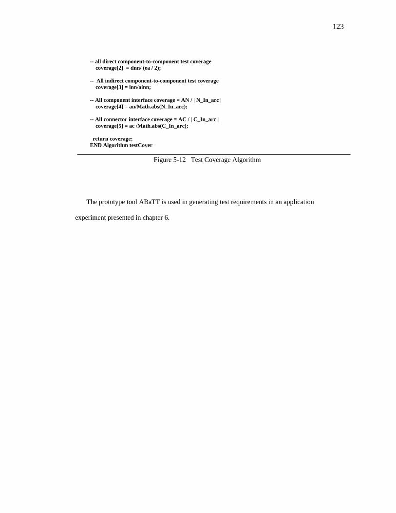
123
-- all direct component-to-component test coverage coverage[2] = dnn/ (ea / 2);
-- All indirect component-to-component test coverage coverage[3] = inn/ainn;
-- All component interface coverage = AN / | N_In_arc | coverage[4] = an/Math.abs(N_In_arc);
-- All connector interface coverage = AC / | C_In_arc | coverage[5] = ac /Math.abs(C_In_arc);
return coverage;END Algorithm testCover
Figure 5-12 Test Coverage Algorithm
The prototype tool ABaTT is used in generating test requirements in an application
experiment presented in chapter 6.

124
Chapter 6 Validation Method and An Application Example
Validation of this research is conducted by applying the testing method developed in this
dissertation to an industrial software system. The goal of the validation is to determine whether
the testing method can detect faults effectively. To facilitate this experiment, the prototype tool
is developed as part of the research to evaluate the proposed test criteria. This chapter presents
the experiment design and discusses the results. Validation for the research is carried out by
developing and executing tests on faulty versions of an industrial software system. This
application experiment is the third part of the solution topology defined in Chapter 1, shown in
Figure 6-1. An actual implementation of a software system described in a specific ADL Wright
is tested using the architecture-based testing technique. Test cases are generated and used to
find faults seeded in the software system.
Figure 6-1 Tests For an Implementation
Part 3
Mapping the ADL Descriptionto the Implementation
An Actual Implementation
Test CasesFor the Implementation
Tests for an Implementation (Chapter 6)
A Specific ADL Description Test Requirements(Defined in Chapter 4)

125
6.1 Experiment Design
The experiment is designed as follows:
Subject Program: An industrial application system was used as the subject program. The
program is written in several programming languages, including Java, C, Perl/CGI, and HTML.
It has nine major components at the architecture level. It contains client-server applications, a
web-based application, file I/O, and pipe-line style processing. The system contains
approximately 2500 lines of code.
Test Adequacy Criteria: Three methods were compared: (1) manual/specification testing
based on experience and requirements specification, (2) the coupling-based integration testing
criteria [JO98], and (3) the architecture-based testing technique discussed in this dissertation.
Test Data: Three sets of test data were generated for each testing method applied on the
subject program. The generation of each test data set is specific to each test method applied.
Fault Set: The research was validated by determining the effectiveness of the software
architecture-based testing criteria at detecting faults that are associated with the connections of
the architecture components. It was necessary to inject faults of architecture related types. We
use the current research results of architectural mismatches classifications by Gacek
[GACEK99, GACEK98]. Their work addresses the importance of underlying architectural
features in determining potential architectural mismatches while composing arbitrary
architecture components. This is not yet an architectural level fault classification, but the
mismatches set does include many typical faults that are likely to occur at the architecture level.
Therefore, we chose to use this study as the source to define faults to be seeded in our subject
program.

126
Measurement: The fault detecting effectiveness of a given test adequacy criteria c for a
given architecture a with respect to a specific fault set f is defined as the ratio of the number of
faults detected to the number of faults seeded. This measurement was made for each pair of
subject architecture program and test adequacy criterion. In this experiment, we have three sets
of test cases for the three testing methods.
Experimental Procedure: The conduct of the experiment consisted of several steps. Let A
be an architecture, C be the test adequacy criteria, and T be the set of test data generated for
each test adequacy criterion.
For each a ∈ A and c ∈ C:
Step 1. Generate c-adequate test data set T(a,c).
Step 2. Define fault set F(a) for a.
Step 3. For each f ∈ F(a) define the fault seeded architecture A(f) by seeding a with
faults, yielding a fault-seeded architecture a(f) where each a(f) ∈ A(f).
Step 4. For each t ∈ T(a,c), if it detects some faults, increase Num(a,c) -- the number of
faults detected by test data set T(a,c). This does not double count if the same
fault is detected by two tests.
Step 5. Determine the fault detection rate R(a, c), for test adequacy criterion c with
respect to architecture a, as:
R(a,c) = Num(a,c) / |F(a,c)|
Step 6. Determine the fault detection effectiveness E(a, c), for test adequacy criterion a
with respect to arachitecture a, as:
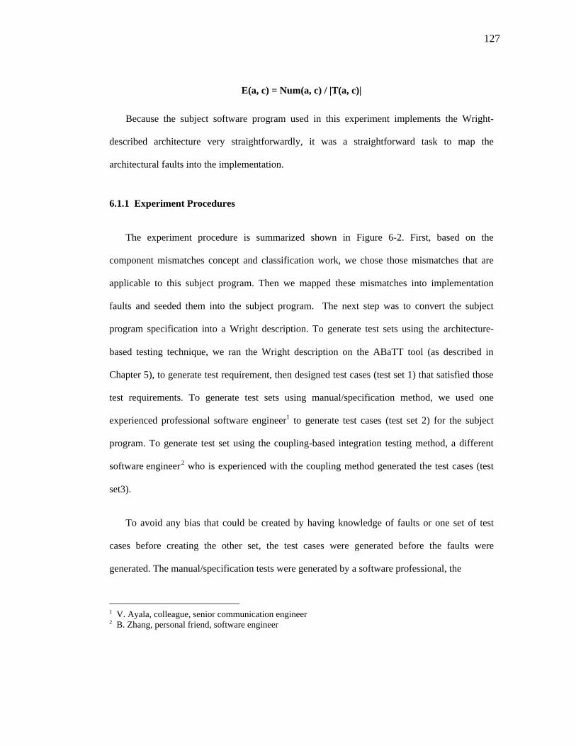
127
E(a, c) = Num(a, c) / |T(a, c)|
Because the subject software program used in this experiment implements the Wright-
described architecture very straightforwardly, it was a straightforward task to map the
architectural faults into the implementation.
6.1.1 Experiment Procedures
The experiment procedure is summarized shown in Figure 6-2. First, based on the
component mismatches concept and classification work, we chose those mismatches that are
applicable to this subject program. Then we mapped these mismatches into implementation
faults and seeded them into the subject program. The next step was to convert the subject
program specification into a Wright description. To generate test sets using the architecture-
based testing technique, we ran the Wright description on the ABaTT tool (as described in
Chapter 5), to generate test requirement, then designed test cases (test set 1) that satisfied those
test requirements. To generate test sets using manual/specification method, we used one
experienced professional software engineer1 to generate test cases (test set 2) for the subject
program. To generate test set using the coupling-based integration testing method, a different
software engineer2 who is experienced with the coupling method generated the test cases (test
set3).
To avoid any bias that could be created by having knowledge of faults or one set of test
cases before creating the other set, the test cases were generated before the faults were
generated. The manual/specification tests were generated by a software professional, the
1 V. Ayala, colleague, senior communication engineer2 B. Zhang, personal friend, software engineer

128
coupling-based tests were generated by another independent software professional, and the
architecture-based testing tests were generated with the support of the prototype tool ABaTT.
Each test case was executed against the faulty-version of the subject program. After each
execution, failures (if any) were checked and corresponding faults were debugged. This process
was repeated on each test case until no more failures occurred. The number of faults detected
was recorded and used in the analysis.
Figure 6-2 Experiment Procedure
Convert Specification toWright Description
Run Prototype Tool
Subject ProgramSpecification
Wright description of the subject program
Test cases for thesubject program (Test set 1)
Run Test Cases on TheFault-seeded Program
Subject ProgramImplementation
SelectedFault Set
Insert Faults to The SubjectProgram Implementation
Fault-seeded program
Manually GenerateTest Cases
Test cases for thesubject program(Test set 2)
Test cases for the subject program(Test set 3)
Apply Coupling-basedTesting Technique
Result 1 Result 2 Result 3
Compare Results
Observation

129
6.1.2 The Subject Program
The subject program is an industrial software system. Because of its proprietary nature, we
can only provide the high level abstract of the program structure, and cannot publish the code.
This software system receives real-time data from external data sources, and processes and
archives selected data. Customers can request some archived data, which will cause the system
to send data that meets the customer's criteria to destination points (external data sinks). An
overview of the system is shown in Figure 6-3. The subject program Wright description is given
in Appendix C. Data Receiver receives the data from the data source and passes it to Data
Packaging Processor where data gets initially processed and readied to send to Data Archiving
Process through networks. Data is archived to data files at the Data Archiving Processor.
Selected data is sent to the User Request Processor through network. User Request Processor
makes system calls through network to the Web Interface Service Program. The system calls
need to use request parameters in the request configuration file. The Web Interface Service
program sends field values to the Web Server Request Handler to check customer request
criteria. Web responses are then shown as web pages. Response information is sent back to the
User Request Processor. The User Request Processor then selects archived data from data
archive 2 and sends it to Data Archiving Processor. Finally, Data Archiving Processor sends
requested data to the Data Packaging Processor for data transmitting to the Data Transmitter,
and eventually to the designated data sink. Currently, Web Interfaces Service communicates
with Web Server Request Handler through CGI program calls. All other network
communications are through TCP/IP socket connection.
There are four benefits for using this subject program. (1) This program reflects all the
architecture relations we described in the testing technique. (2) The subject program is simple

130
enough that most of the code deals with communications/connections between components.
Even though the implementation is at the unit level, it shows only connections that are at the
system level. (3) The subject program code is written in more than one language. JAVA, Perl,
Javascript, HTML, and C languages are used in this system. Data Receiver and Data
Transmitter components are written in C. Data Packaging, and Data Archiving are written in
Java. User Request is written in Java, HTML, and Perl. Web Interface, Perl Socket, and Web
Server are written in Javascript, Perl and HTML. This shows that the component integration can
be based on different language components. (4) Internet protocols are used in the system, which
adds another complication to the subject system.
Figure 6-3 The Subject Program
Data Receiver Data Transmitter
Data PackagingProcessor
Data ArchivingProcessor
User RequestProcessor
Web InterfaceService
Web ServerRequest Handler
Data Archive 1
RequestConfig File
Data Archive 2
Data sinkData source
Internet
Networks
Networks
Networks
File I/O
File I/O
File I/O
data data
data
data
data
data
System call
response
Response web page
CGI form field values
Perl Socket response

131
6.1.3 Test Adequacy Criteria
We use three types of test adequacy criteria in this experiment application. (1) In the
manual/specification method, test requirements are generated based on the specification of the
subject program. A brief system specification of the subject system was available, where high
level data flow and control flow were presented. Test requirements and test cases were
generated based on the data flow, control flow, as well as the text description. (2) The coupling-
based testing technique is an integration testing technique [JO98] that is based on the couplings
between software components. Coupling between two program units increases the
interconnections between the two units and increases the likelihood that a fault in one unit may
affect others. The coupling-based testing criteria are based on the design and data structures of
the program, and on the data flow between the program units. This technique requires that the
program execute from definitions of actual parameters (coupling-defs) through calls to uses of
the formal parameters (coupling-uses). Four levels of testing criteria are defined: call-coupling,
all-coupling-defs, all-coupling-uses, and all-coupling-paths. In this experiment application, we
chose to use all-coupling-path coverage criterion, the highest level of the four, which requires
that for each coupling-def of variable x, the set of paths executed by test set T contains all paths
from the coupling-def to all reachable coupling-uses. Test cases are generated to meet this
criterion. (3) For the software architecture-based testing technique, we used the all indirect
component-to-component coverage criterion to generate test requirements using the prototype
tool ABaTT.
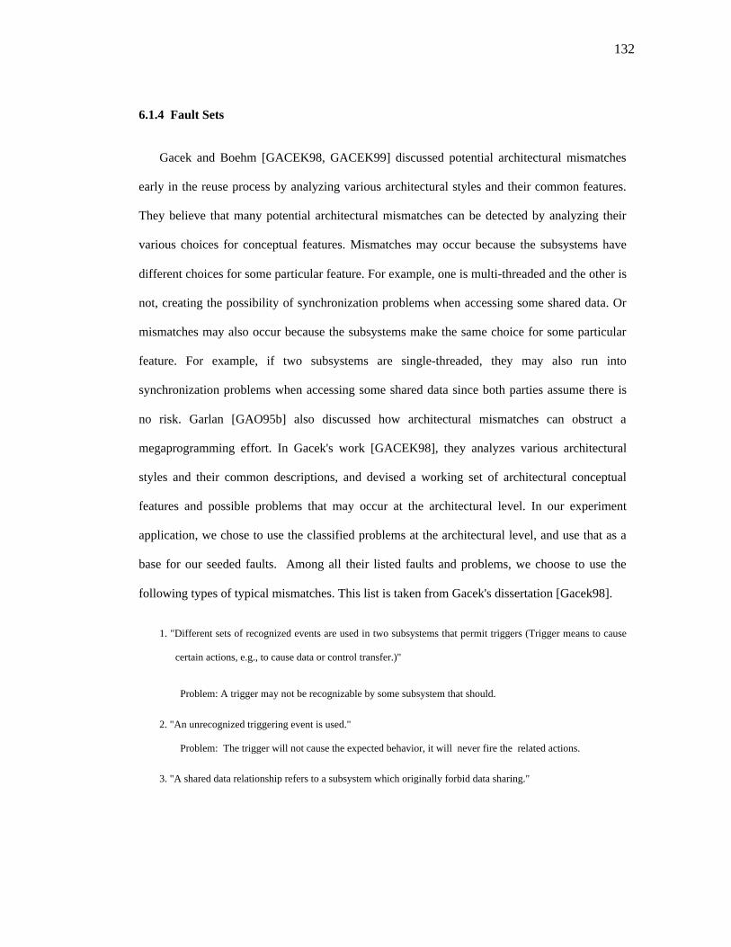
132
6.1.4 Fault Sets
Gacek and Boehm [GACEK98, GACEK99] discussed potential architectural mismatches
early in the reuse process by analyzing various architectural styles and their common features.
They believe that many potential architectural mismatches can be detected by analyzing their
various choices for conceptual features. Mismatches may occur because the subsystems have
different choices for some particular feature. For example, one is multi-threaded and the other is
not, creating the possibility of synchronization problems when accessing some shared data. Or
mismatches may also occur because the subsystems make the same choice for some particular
feature. For example, if two subsystems are single-threaded, they may also run into
synchronization problems when accessing some shared data since both parties assume there is
no risk. Garlan [GAO95b] also discussed how architectural mismatches can obstruct a
megaprogramming effort. In Gacek's work [GACEK98], they analyzes various architectural
styles and their common descriptions, and devised a working set of architectural conceptual
features and possible problems that may occur at the architectural level. In our experiment
application, we chose to use the classified problems at the architectural level, and use that as a
base for our seeded faults. Among all their listed faults and problems, we choose to use the
following types of typical mismatches. This list is taken from Gacek's dissertation [Gacek98].
1. "Different sets of recognized events are used in two subsystems that permit triggers (Trigger means to cause
certain actions, e.g., to cause data or control transfer.)"
Problem: A trigger may not be recognizable by some subsystem that should.
2. "An unrecognized triggering event is used."
Problem: The trigger will not cause the expected behavior, it will never fire the related actions.
3. "A shared data relationship refers to a subsystem which originally forbid data sharing."

133
Problem: May cause synchronization problems.
4. "There is a non-deterministic set of actions that could be caused by a trigger event."
Problem: It is not clear which set of actions should actually occur when triggered, and also it is not clear
what the action ordering should be.
5. "Data connectors connecting control components that are not always active may lead into deadlock."
Problem: Possibility of deadlock on the control component sending the data.
6. "Call to a cyclic (non-terminating) subsystem/control component."
Problem: Control will never be returned to the caller.
7. "Call to a private method."
Problem: Method not accessible to the caller.
8. "Sharing private data."
Problem: Data not accessible to all of the sharing entities being composed.
9. "A reentrant component is either sending or receiving a data transfer."
Reentrance means that some systems allow for multiple simultaneous, interleaved, or nested invocations of
the same piece of code that will not interfere with each other.
Problem: Potential incorrect assumption of which invocation of a component is either sending or
receiving a data transfer.
10. "Call to a non-reentrant component."
Problem: Component may already be running.
11. "Call from a subsystem requiring some predictable response times to some component(s) not originally
considered."
Problem: May have side effects on original predicted response times.
12. "Only part of the resulting system automatically reconfigures upon failure."
Problem: When other parts do not reconfigure, the system may not run correctly.
13. "Incorrect assumption of which instantiation of an object is either sending or receiving a data
transfer."

134
14. "Time represented/compared using different granularities."
Problem: Communications concerning time cannot properly occur.
15. "Sharing or transferring data with differing underlying representations."
Problem: Communications concerning the specific data will not properly occur.
16. "Resource contention."
Problem: Predictable response time indirectly affected because there may be some resource
contention not originally considered.
Based on the above 16 problems that can occur in the composition of two subsystems, we
created the following 16 faults for our subject system. The faults shown in Table 6-1 were
manually inserted to the subject program.
Table 6-1 Faults Inserted to the Subject Programs
FaultType
Faults in the Subject Programs
1. A wrong trigger event in the Perl program.2. A fault in the JavaScript program that does not cause to trigger the response event.3. File reading and file writing in different format before archiving and after archiving.4. In Data Packaging Processor, the run program has the wrong conditions to start the process or
to end the process.5. A wrong data transfer between a client and a server, causing other part of the program
deadlocked.6. Use (datastream != null) instead of (moredata !=null) to check socket connection, this causes
the run program to never stop even when there is no data transfer.7. A private method is called from outside.8. Wrong use of a private data.9. Wrong assumption of the invocation party between a client and a server component.10. Multiple calls to the same server port number while the sever port is already in use.11. Set wait_for_response_time very short when waiting for web server responses. This leads the
program to raise an exception when a response does not come back within the desired timelimit.
12. Set some clients automatically reconnect to the server when the server is down, and set otherclients to not to reconnect.
13. The sequence of operation in the server-client relations is incorrect.14. Calculate current time based on minutes instead of seconds. This causes problems when the
time difference is within a minute.15. Security certificate contention when there are multiple URL requests.16 Incompatible port numbers between a server and a client component.

135
6.2 Experimental Results
Following the experiment procedures described in Figure 6-2, first we generated the Wright
description of the application program, which is shown in Appendix C. The ICG of the subject
program system is shown in Figure 6-3. Some of the behavior graphs are given in Appendix D.
Test requirements in terms of BG paths are listed in Appendix C. There are 9 components, 9
connectors and links between components and connectors. Ports of components use names
proceeded with "p", and roles use names proceeded with "r". The ICG is shown in Figure 6-4.
Figure 6-4 The ICG of the Subject Program
ReceiverReceiver-Packaging Packaging
p1
p1
p2
Archiving
Transmitter
p1
Transmitter-Packaging
p1
p3
UserRequest
ConfigWebInterf
WebServer
Packaging-Archiving
WebInterf -WebServer
WebInterf-UserRequest
UserRequest-Config
Archiving-UserRequest
p1 p2
p3 p4
p1
p2 p3
p4
r1 r2r4
r1 r2
p2
r1
r1
r1
r2
r3
r2
p1
p3
r2
r1
p1
r2
p2
r1
r2p1
r1
r2
r1
r2
PERL
WebInterf -PERL
PERL-UserRequest

136
Observed test results are shown in table 6-2 and Table 6-3.
Table 6-2 Test Results
FaultNumber
Architecture-basedTesting TechniqueTest Set 1
Manual/SpecificationMethodTest Set 2
Coupling-basedTesting TechniqueTest Set 3
1 Found Found Not Found2 Found Found Not Found3 Not Found Not Found Found4 Found Not Found Not Found5 Found Found Not Found6 Found Found Not Found7 Found Found Found8 Not Found Not Found Found9 Found Found Found10 Found Not Found Not Found11 Found Found Not Found12 Found Found Found13 Found Found Found14 Found Found Not Found15 Found Found Found16 Found Found Found
Table 6-3 Faults Detected
Architecture-based Manual/specification Coupling-basedNumber of TestCases
24 21 14
Faults Found 14 10 8Faults Not Found 2 6 8Fault-foundPercentage R(a, c)
87.5% 62.5% 50.0%
Test EffectivenessE(a, c)
58.3% 47.6% 57.1%
From Table 6-3 it can be seen that the architecture-based technique resulted in 24 test cases,
which detected 14 faults. Fault 3 is a unit level fault, which only affects the content of the data

137
file, but is not shown anywhere else. Fault 8 is the wrong use of a private data object, which
also affects the content of the data transferred. These two faults were not found because they are
not demonstrated at the architectural level. The manual/specification method resulted in 21 test
cases, which detected 10 faults. Four faults were not found. Fault 3 was discussed above. Fault
4 is a wrong start process condition that causes incorrect data transfer sequences, but still keeps
the whole system up and running. Fault 8 is the wrong use of a private data, which only affects
the content of the data transferred. Fault 10 is a multiple calling to a port number that is already
in use, this fault causes a wrong data transfer, but is not visible at the system level. The port
ordering rules helped to generate test cases that checked the ordering sequence of the port
invocation, allowing the architecture-based testing technique to detect the faults. The coupling-
based technique resulted in 14 test cases, which detected 8 faults. All 8 faults that were not
found are the ones that are not covered by the all-coupling-paths.
The goal of this experiment was twofold. One is to see if architecture-based testing could be
practically applied. The second was to make a preliminary evaluation of the merit of the
architecture-based technique by comparing it with the coupling-based method and the
manual/specification method. From the experiment results we conclude that the goals were
satisfied; the architecture-based testing technique was applied and worked fine, and performed
better than the other two techniques. However, there are several limitations to the interpretation
of the results. First, the subject program is of moderate size for industrial applications, it has
only several architecture styles in the system. Larger sized and more complicated systems need
to be used. Second, there is a lack of the classification of faults at the architectural level. Our
seeded faults in the subject program were derived from a subsystem-based composition
mismatches list. The faults we used in the subject program may not cover all the typical faults at

138
the architectural level. An architectural fault classification is needed for further experiment.
Third, since there is a lack of formal architectural/system testing technique, we used the
coupling-based integration testing technique as one of the comparison technique. Other system
or architectural testing technique should be compared with our technique. Fourth, only one
ADL description is used to describe the system. Other architecture description languages should
also be applied.
6.3 Conclusion
From this experiment application, we can see that the architecture-based testing technique
can be practically applied, and the preliminary evaluation shows that it can find architectural
level faults effectively. This result indicates that this testing approach can benefit practitioners
who are performing architecture/system testing on software. More evaluation of the
effectiveness of this technique is necessary for future work.

139
Chapter 7 Contributions and Future Research
This dissertation has presented six major new results. First, a new general testing technique
for software architecture-based testing has been defined and developed. The research led to the
creation of a set of new concepts including the software architecture Interface Connectivity
Graph (ICG), architecture relations, software architecture-based testing requirements,
architecture-based testing criteria and testing coverage. Second, properties that need to be
evaluated at the software architecture level have been defined. We classified the different
architecture relations in the software architecture context, and the different testing requirements
that have to be satisfied in testing at software architecture level. These concepts are formally
defined. Third, general architecture-based testing criteria are formally defined and test coverage
analysis is presented to help users to evaluate how much of the architecture specification has
been tested using this testing technique. Forth, these testing criteria have been instantiated to a
specific ADL, Wright. Based on the particular characteristics of Wright specifications, the
architecture Behavior Graph (BG) is introduced to graphically represent the behavior details and
other properties to be tested for a Wright specification. Transformation rules are presented to
map a Wright description to the ICG and the BG representations, and architecture relations are
connected with the Petri Net based architecture modeling technique so as to utilize many of the
developed Petri Net algorithms and analysis techniques. Fifth, algorithms are defined to
automatically generate test cases for Wright Description using the software architecture-based

140
testing technique. These algorithms can generate test cases for any given defined testing
criteria. Sixth, a proof-of-concept tool has been implemented and used validate this approach
on industrial software.
By using the technique developed in this research to testing software architecture, we hope
to be able to get information about architecture and start testing software systems as early as
when they are in the architectural design stage. This technique can provide visual tools (such as
Petri Nets) into testing, modeling and simulation of the architecture properties at a higher level
of abstraction. Architecture-based testing criteria are used as guidelines and they can be applied
to automatically generate test cases for a given ADL. Tests and the intermediate graphical
representations (BGs) can be used as guidelines in the detail design and later in the actual
implementation. This allows significant testing activities to be carried out early in the software
development process, and can greatly reduce the risks of the propagation of costly errors
because the later the errors are discovered the more they cost. As a result, it can help software
developers design test early and reuse the tests later in the software development process. The
concept of architecture relations and the testing criteria can be used both at the architecture level
as well as refined with more design information so that they can be applied at design and
implementation stages. This is also a general testing technique that can be applied to various
ADLs.
Future Research
There are several future areas to explore. First, we applied this technique only to one ADL,
Wright. In the next research step, we would like to apply this technique to other ADLs such as

141
Rapide, Darwin, and etc. Applications to other ADLs should further help us to see the
effectiveness of this technique. Second, we could refine our research by studying the
transformation of Wright state variables and other constraints to the BG to find and overcome
any possible limitations on the translation. Third, more research can be carried out in the
analyzing of software architectures. As we pointed out in Chapter 2, properties such as
consistency, deadlock, completeness need to be checked as we carry out testing and analysis at
the architecture level. Theories and algorithms developed for Petri Nets can be applied. Another
direction is to test dynamic aspects of software architectures. This issue is not addressed in this
dissertation.

142
APPENDIX A WRIGHT LANGUAGE IN BNF
This appendix gives the Wright language in the form of BNF. This is fromhttp://www.cs.cmu.edu/afs/cs/project/able/www/wright/wright_tools.html.
SpecList := Spec | SpecList Spec;Spec := Configuration | Style;
Style := "Style" SimpleName[ TypeList ][ "Constraints"
[ ConstraintExpression ] ]"End Style";
TypeList := Type | TypeList Type ;Type := Component | Connector | InterfaceType | GeneralProcess;
Component := "Component" SimpleName [ '(' FormalCCParams ')' ] [ PortList ]"Computation" BehaviorDescription;
Connector := "Connector" SimpleName [ '(' FormalCCParams ')' ][ RoleList ]"Glue" BehaviorDescription;
PortList := Port | PortList Port;Port := "Port" FormalPRName '=' ProcessExpression;
RoleList := Role | RoleList Role;Role := "Role" FormalPRName '=' ProcessExpression;
Configuration:= "Configuration" SimpleName[ "Style" SimpleName ][ TypeList ]"Instances" [ InstanceList ]"Attachments" [ AttachmentList ]"End Configuration";
InstanceList := Instance | InstanceList Instance;Instance := NameList ':' TypeUse;

143
TypeUse := SimpleName [ '(' ActualCCParams ')' ];
AttachmentList := Attachment | AttachmentList Attachment;Attachment : Interface "As" Interface;Interface : SimpleName '.' ActualPRName;
InterfaceType:= "Interface Type" ProcessName '=' ProcessExpression;GeneralProcess:= "Process" ProcessName '=' ProcessExpression;
Names and Lists
• IDENTIFIER is a terminal representing an arbitrary name. Such names can contain ancombination of letters and digits, but must begin with a letter.
SimpleName := IDENTIFIER;ProcessName := SimpleName [ "_{" ProcessParams '}' ]AlphabetName := "ALPHA" SimpleName;DefnName := ProcessName | AlphabetName;
NameList := SimpleName | NameList ',' SimpleName;ElementList := DataExpression | ElementList ',' DataExpression;
FormalPRName := SimpleName [ "_{" FiniteRangeExpression '}' ];ActualPRName := SimpleName [ "_{" IntegerExpression '}' ];
EventName := [ ActualPRName '.' ] SimpleName
BehaviorDescription := '=' ProcessExpression| Subconfiguration;
Subconfiguration := Configuration "Bindings" [ BindingList ] "End Bindings"
BindingList := Binding | BindingList Binding;Binding := Interface '=' ActualPRName;
DeclList := Declaration | DeclList Declaration;Declaration :=
DefnName '=' AnyExpression| DefnName '=' "Cond" '{' ConditionalDefinitions '}'
ConditionalDefinitions =ConditionalDefinition| ConditionalDefinitions ConditionalDefinition
ConditionalDefinition =ProcessExpression "When" '{' LogicalExpression '}'

144
| ProcessExpression "Otherwise"
Types of parameters (formal and actual for use in various rules)
The NL variant of ForamlParams allows lists of parameters, but each parameter of thesame type must be specified separately instead of in a list of the same type (eg, "i,j:X" isnot permitted; instead "i:X; j:X" would have to be used).
FormalParams := FormalParam | FormalParams ';' FormalParam;FormalParam := NameList ':' SetExpression;
FormalParamsNL := FormalParamNL | FormalParamsNL ';' FormalParamNL;FormalParamNL := SimpleName ':' SetExpression;
ProcessParams := AnyExpression | ProcessParams ',' AnyExpression;
FormalCCParams := FormalCCParam | FormalCCParams ';' FormalCCParam;FormalCCParam := NameList ':' ProcessType | NameList ':' RangeExpression;
ActualCCParams := ActualCCParam | ActualCCParams ',' ActualCCParam;ActualCCParam := ProcessExpression | IntegerExpression;
types of expresssions
ProcessType :="Interface Type"| "Process"| "Port"| "Role"| "Computation"| "Glue";
ProcessExpression := ProcessExpression ';' ProcessExpression | ProcessExpression "/\" ProcessExpression
| EventExpression "->" ProcessExpression | ProcessExpression "||" ProcessExpression
| ProcessExpression "|||" ProcessExpression | ProcessExpression "[]" ProcessExpression | ProcessExpression "|~|" ProcessExpression | "[]" FormalParams '@' ProcessExpression | "|~|" FormalParams '@' ProcessExpression | ';' FormalParams '@' ProcessExpression | "||" FormalParams '@' ProcessExpression
| "|||" FormalParams '@' ProcessExpression| ToolAnnotation
| ProcessName | "Computation" | "Glue"
| "Success"
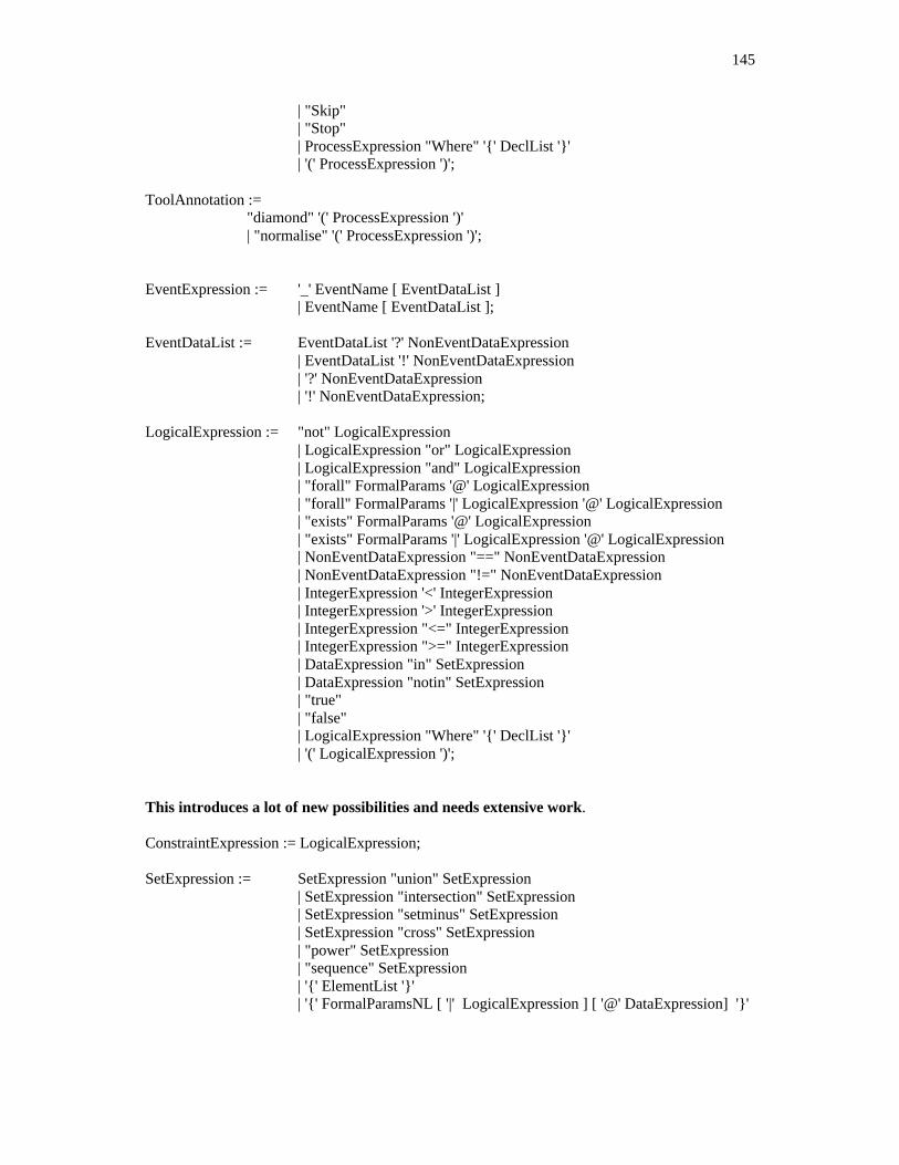
145
| "Skip"| "Stop"
| ProcessExpression "Where" '{' DeclList '}' | '(' ProcessExpression ')';
ToolAnnotation := "diamond" '(' ProcessExpression ')'
| "normalise" '(' ProcessExpression ')';
EventExpression := '_' EventName [ EventDataList ] | EventName [ EventDataList ];
EventDataList := EventDataList '?' NonEventDataExpression| EventDataList '!' NonEventDataExpression| '?' NonEventDataExpression| '!' NonEventDataExpression;
LogicalExpression := "not" LogicalExpression | LogicalExpression "or" LogicalExpression | LogicalExpression "and" LogicalExpression | "forall" FormalParams '@' LogicalExpression | "forall" FormalParams '|' LogicalExpression '@' LogicalExpression | "exists" FormalParams '@' LogicalExpression | "exists" FormalParams '|' LogicalExpression '@' LogicalExpression
| NonEventDataExpression "==" NonEventDataExpression| NonEventDataExpression "!=" NonEventDataExpression
| IntegerExpression '<' IntegerExpression | IntegerExpression '>' IntegerExpression | IntegerExpression "<=" IntegerExpression | IntegerExpression ">=" IntegerExpression | DataExpression "in" SetExpression | DataExpression "notin" SetExpression
| "true"| "false"
| LogicalExpression "Where" '{' DeclList '}' | '(' LogicalExpression ')';
This introduces a lot of new possibilities and needs extensive work.
ConstraintExpression := LogicalExpression;
SetExpression := SetExpression "union" SetExpression | SetExpression "intersection" SetExpression | SetExpression "setminus" SetExpression | SetExpression "cross" SetExpression | "power" SetExpression
| "sequence" SetExpression | '{' ElementList '}' | '{' FormalParamsNL [ '|' LogicalExpression ] [ '@' DataExpression] '}'

146
| RangeExpression| SimpleName| AlphabetName| "Integer"| "{}"
| SetExpression "Where" '{' DeclList '}'| '(' SetExpression ')';
SequenceExpression := '<' ElementList '>' | SequenceExpression '^' SequenceExpression | SimpleName | "<>"
| SequenceExpression "Where" '{' DeclList '}' | '(' SequenceExpression ')';
IntegerExpression := IntegerExpression '+' IntegerExpression | IntegerExpression '-' IntegerExpression | SimpleName
| INTEGER | IntegerExpression "Where" '{' DeclList '}' | '(' IntegerExpression ')';
RangeExpression := IntegerExpression ".." IntegerExpression | IntegerExpression ".." | ".." IntegerExpression;
FiniteRangeExpression := IntegerExpression ".." IntegerExpression
TupleExpression := '(' DataExpression ',' DataExpression ')';
NonEventDataExpression := SetExpression
| IntegerExpression| SequenceExpression| LogicalExpresssion| TupleExpression;
DataExpression := EventExpression | NonEventDataExpression;
AnyExpression := ProcessExpression | DataExpresssion;

147
APPENDIX B WRIGHT PROCESSES AND EVENTS
e: event
e?x: Process receives data x
e!x: process supplies data x
§: successful termination of the entire system
e P: the process that first engages in the event e and then behaviors as P
p: external choice. A process that can behave like P or Q, where the choice is made by the
environment, is denoted by the operator P Q
Π: internal choice. A process that can behave like P or Q, where the choice is made (non-
deterministically) by the process itself, is denoted P Q.
; : the ";" operator combines two processes in sequence. P;Q is the process that behaves as
P until P terminates successfully and then behaves as Q.
where: behavior patterns that occur over and over again can be described by naming
particular processes.
state variable: state is added to a process definition by adding subscripts to the name of a
process: Pi is a process with a single state variable, i.

148
APPENDIX C SUBJECT PROGRAM WRIGHT DESCRIPTIONSAND TESTS
This appendix lists the Wright description of the subject program, lists all the test path
requirements generated by architecture-based testing technique, lists all the test requirements by
manual method as well as by coupling-based method.
Wright Description of the Subject Program
Interface Type ClientAction = open Operate §where Operate = setConnection Operate connectResponse?x ReadOrWrite Operate EndReadOrWrite = writeToSocket ReadOrWrite readFromSocket ReadOrWrite End = close § fail §
Interface Type ServerAction = open Operate § where Operate = listenOnPort Operate connectResponse!x ReadOrWrite Operate End
ReadOrWrite = writeToSocket ReadOrWrite readFromSocket ReadOrWriteClose = close § fail §
Interface Type SendCGIForm = openURL ; SubmitOrExitwhere SubmitOrExit = submitValues?f SucceedOrFail ExitSucceedOrFail = responsePage!y closefile § fail ToSubmit §Exit = failOpenURL §
Interface Type AcceptCGIForm = openFile Check §Check = checkFieldNames!f SucceedOrFail § ExitSucceedOrFail = responsePage?y closefile § fieldNotMatch §Exit = failOpenFile §
Interface Type FileIO = openFile; NextActionwhere NextAction = writeToFile NextAction readFromFile NextAction fileFail §
closeFile § failOpenFile §

149
Component ReceivingPort p1 = ClientAction
Computation
Component TransmittingPort p1 = ServerAction
Computation
Component PackagingPort p1 = ServerActionPort p2 = ServerActionPort p3 = ClientActionPort p4 = ClientActionComputation = ( x: 1..2 px.open); ConnectOrExit
where ConnectOrExit = Connect ExitConnect = ( x: 1..2 px.listenOnPort Connect) ; ( x: 1..2 ; processx.); SendDataprocess1 = p1.connectResponse!x p4.open Operate Exitwhere Operate = p1.setConnection Operateprocess2 = p2.connectResponse!x p3.open Operate Exitwhere Operate = p3.setConnection OperateSendData = p1.readFromSocket p4.writeToSocket SendDataExit = Fail §Fail = ( x: 1..4 px.failOpen) §
Component ArchivingPort p1 = ServerAction
Port p2 = ServerActionPort p3 = ClientActionComputation = ( x: 1..2 px.open); ConnectOrExit
ConnectOrExit = Connect ExitConnect = ( x: 1..2 px.listenOnPort Connect) ; ( x: 1..2 ; processx.); SendDataprocess1 = p1.connectResponse!x p3.open Operate ExitOperate = p3.setConnection Operateprocess2 = p2.connectResponse!xSendData = p1.readFromSocket p2.writeToSocket p2.readFromSocket p3.writeToSocketExit = ( x: 1..3 px.failOpen) § ( x: 1..3 ; px.close); §
Component UserRequestPort p1 = ServerAction
Port p2 = ClientActionPort p3 = SendCGIFormPort p4 = FileIOComputation = ( x: 1..2 px.open); ConnectOrExitConnectOrExit = Connect ExitConnect = ( x: 1..2 px.listenOnPort Connect) ; ( x: 1..2 ; processx.); SendDataprocess1 = p1.connectResponse!x p3.open Exitprocess2 = p2.connectResponse!xSendData = p2.readFromSocket p4.writeToFile p 4.closeFile p 3.openURL p 3.responsePage p1.writeToSocket p1.readFromSocket p2.writeToSocketExit = ( x: 1..4 px.failOpen) § ( x: 1..4 ; px.close); §
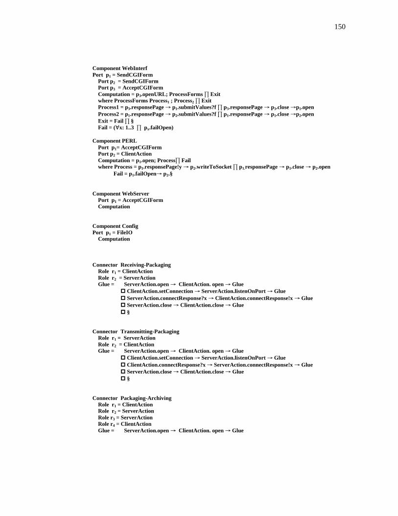
150
Component WebInterfPort p1 = SendCGIForm
Port p2 = SendCGIFormPort p3 = AcceptCGIFormComputation = p3.openURL; ProcessForms Exitwhere ProcessForms Process1 ; Process2 ExitProcess1 = p3.responsePage p1.submitValues?f p3.responsePage p3.close p1.openProcess2 = p1.responsePage p2.submitValues?f p1.responsePage p1.close p2.openExit = Fail §Fail = ( x: 1..3 px.failOpen)
Component PERLPort p1= AcceptCGIFormPort p2 = ClientActionComputation = p1.open; Process Failwhere Process = p1.responsePage!y p2.writeToSocket p1.responsePage p1.close p2.open Fail = p1.failOpen p2.§
Component WebServerPort p1 = AcceptCGIFormComputation
Component ConfigPort p1 = FileIO
Computation
Connector Receiving-PackagingRole r1 = ClientActionRole r2 = ServerActionGlue = ServerAction.open ClientAction. open Glue
ClientAction.setConnection ServerAction.listenOnPort Glue ServerAction.connectResponse?x ClientAction.connectResponse!x Glue ServerAction.close ClientAction.close Glue §
Connector Transmitting-PackagingRole r1 = ServerActionRole r2 = ClientActionGlue = ServerAction.open ClientAction. open Glue
ClientAction.setConnection ServerAction.listenOnPort Glue ClientAction.connectResponse?x ServerAction.connectResponse!x Glue ServerAction.close ClientAction.close Glue §
Connector Packaging-ArchivingRole r1 = ClientActionRole r2 = ServerAction
Role r3 = ServerActionRole r4 = ClientActionGlue = ServerAction.open ClientAction. open Glue

151
ClientAction.setConnection ServerAction.listenOnPort Glue ClientAction.connectResponse?x ServerAction.connectResponse!x Glue ServerAction.close ClientAction.close Glue §
Connector Archiving-UserRequestRole r1 = ServerActionRole r2 = ClientActionGlue = ServerAction.open ClientAction. open Glue
ClientAction.setConnection ServerAction.listenOnPort Glue ClientAction.connectResponse?x ServerAction.connectResponse!x Glue ServerAction.close ClientAction.close Glue §
Connector WebInterf-UserRequestRole r1 = SendCGIFormRole r2= AcceptCGIFormGlue = SendCGIForm.openURL AcceptCGIForm.openFile Glue
SendCGIForm.submitFormValues?f AcceptCGIForm.checkFieldNames!f Glue AcceptCGIForm.responsePage!y SendCGIForm.responsePage?y Glue
AcceptCGIForm.failOpen SendCGIForm.failToSubmit Glue §
Connector WebInterf-WebServerRole r1 = SendCGIFormRole r2 = AcceptCGIFormGlue = SendCGIForm.openURL AcceptCGIForm.openFile Glue
SendCGIForm.submitFormValues?f AcceptCGIForm.checkFieldNames!f Glue AcceptCGIForm.responsePage!y SendCGIForm.responsePage?y Glue
AcceptCGIForm.failOpen SendCGIForm.failToSubmit Glue §
Connector UserRequest-ConfigRole r1 = FileIORole r2 = FileIOGlue
Connector WebInterf-PERLRole r1 = AcceptCGIFormRole r2 = SendCGIFormGlue = SendCGIForm.openURL AcceptCGIForm.openFile Glue
SendCGIForm.submitValues?f AcceptCGIForm.checkFieldNames!f Glue AcceptCGIForm.responsePage SendCGIForm.responsePage Glue
AcceptCGIForm.failOpen SendCGIForm.failToSubmit Glue §
Connector PERL-UserRequestRole r1 = ClientActionRole r2 = ServerActionGlue = ServerAction.open ClientAction. open Glue

152
ClientAction.setConnection ServerAction.listenOnPort Glue ClientAction.connectResponse?x ServerAction.connectResponse!x Glue ServerAction.close ClientAction.close Glue §
Instancesreceiver: Receivingpackaging: Packagingr-p: Receiving-Packaging
archiving: Archivingp-a : Packaging-Archivingtransmitting: Transmittingt-p: Transmitting-Packaginguserrequest: UserRequesta-u: Archiving-UserRequestconfig: Configu-c: UserRequest-Configperl: PERLp-u: PERL-UserRequestwebinterf: Webinterfw-u: WebInterf-UserRequestw-p: WebInterf-PERLwebserver: WebServerw-w: WebInterf-WebServer
Attachments:receiving provides as r-p.receiving
s provides as cs.Send

153
Individual Component Interface Coverage Paths
First, we define all the B-paths for individual ports. These paths will be used in the coverage
requirements.
acceptCGIForm_path:
1. openFile -- checkFieldNames -- reponsePage -- close -- §1
2. openFile -- checkFieldNames -- fieldNotMatch-- close -- §2
3. openFile -- failOpenFile -- §3
4. openFile -- close -- §4
sendCGIForm_path
1. openURL -- submitValues?f -- responsePage -- close -- §1
2. openURL -- submitValues?f -- failToSubmit-- close -- §2
3. openURL -- failOpen -- §3
4. openURL-- close -- §4
FileIO_path:
1. openFile -- close-- §2
2. openFile -- failOpen -- §1
3. openFile -- readFromFile --close -- §2
4. openFile -- WriteToFile -- close -- §2
5. openFile -- readFromFile --WriteToFile --close -- §2
6. openFile -- WriteToFile --readFromFile -- close -- §2
7. openFile -- readFromFile -- failOpen -- §1
8. openFile -- WriteToFile -- failOpen -- §1
9. openFile -- readFromFile --WriteToFile --failOpen -- §1
10. openFile -- WriteToFile --readFromFile -- failOpen -- §1
server_path
1. open -- listenOnPort -- close -- §2
2. open -- close -- §2

154
3. open -- fail -- §3
4. open -- listenOnPort -- connectResponse!x -- readFromSocket -- close -- §2
5. open -- listenOnPort -- connectResponse!x -- writeToSocket -- close -- §2
6. open -- listenOnPort -- connectResponse!x -- readFromSocket --writeToSocket-- close --
§2
7. open -- listenOnPort -- connectResponse!x -- writeToSocket --readFromSocke-- close -- §2
8. open -- listenOnPort -- fail -- §3
9. open -- listenOnPort -- connectResponse!x -- readFromSocket -- fail -- §3
10. open -- listenOnPort -- connectResponse!x -- writeToSocket -- fail -- §3
11. open -- listenOnPort -- connectResponse!x -- readFromSocket --writeToSocket-- fail -- §3
12. open -- listenOnPort -- connectResponse!x -- writeToSocket --readFromSocke-- fail -- §3
13. §1
client_path
1. open -- setConnection -- close -- §2
2. open -- close -- §2
3. open -- fail -- §3
4. open -- setConnection -- connecResponse?x -- readFromSocket -- close -- §2
5. open -- setConnection -- connecResponse?x -- writeToSocket -- close -- §2
6. open -- setConnection -- connecResponse?x -- readFromSocket -- writeToSocket -- close -- §2
7. open -- setConnection -- connecResponse?x -- writeToSocket -- readFromSocket -- close -- §2
8. open -- setConnection -- connecResponse?x -- readFromSocket -- fail-- §3
9. open -- setConnection -- connecResponse?x -- writeToSocket -- fail-- §3
10. §1
Here are the individual components and their B-paths and C-paths:
Receiving:
B-path: client_path
I-path: ∅
Packaging
B-path:

155
port1: server_path
port2: server_path
port3: client_path
port4: client_path
I-path :
Packaging I-path(p1, p4):
1. p1.connectResponse!x -- p4.open
2. p1.readFromSocket -- p4.writeToSocket
Packaging I-path(p2, p3):
1. p2.connectResponse!x -- p3.open
2. p2.readFromSocket -- p3.writeToSocket
Archiving
B-path:
port1: server_path
port2: server_path
port3: client_path
I-path:
Archiving I-path(p1,p3):
1. p1.connectResponse!x -- p3.open
Archiving I-path(p1,p2):
1. p1.readFromSocket -- p2.writeToSocket
Archiving I-path(p2,p3):
1. p2.readFromSocket -- p3.writeToSocket
UserRequest
B-path:
port1: server_path
port2: client_path
port3: sendCGIForm_path
port4: FileIO_path
I-path:

156
UserRequest I-path(p2,p4)
1. p2.connectResponse?x -- p4.openFile
2. p2.readFromSocket -- p4.writeToFile
UserRequest I-path(p4,p3):
1. p4.close -- p3.openURL
UserRequest I-path(p3,p1):
2. p3.responsePage -- p1.writeToSocket
UserRequest I-path(p1,p2):
1. p1.readFromSocket -- p2.writeToSocket
PERL
B-path:
port1: AcceptCGIForm_path
port2: client_path;
I-path:
PERL I-path(p1,p2):
1. p1.responsePage -- p2.writeToSocket
2. p1.close -- p2.open
WebInterf
B-path:
port1: sendCGIForm_path;
port2: sendCGIForm_path;
port3: AcceptCGIForm_path;
I-path:
WebInterf I-path(p3,p1):
1. p3.responsePage -- p1.submitValues?f
2. p3.close -- p1.openURL
WebInterf I-path(p1,p2):
1. p1.responsePage -- p2.submitValues?f

157
2. p1.close -- p2.openURL
Transmitting
B-path: server_path
I-path: ∅
Config
B-path: FileIO_path
I-path: ∅
WebServer
B-path: AcceptCGIForm_path;
I-path : ∅
Individual Connector Coverage
Under current assumptions, all the roles are considered to have the same behavior as their
corresponding component ports. Therefore, the individual connector coverage shares the same B-
path as the individual component coverage.
All Direct Component-to-Component Coverage
Receiving and Packaging
C-path(Packaging.p1, Receiving.p1):
1.Packaging.p1.open -- Receiving.p1. open
2. Packaging.p1.connectResponse!x -- Receiving.p1.connectResponse?x
3. Packaging.p1.close -- Receiving.p1.close

158
C-path(Receiving.p1, Packaging.p1):
1. Receiving.p1.setConnection -- Packaging.p1.listenOnPort
Packaging and Transmitting
C-path(Transmitting.p1, Packaging.p3):
1.Transmitting.p1.open -- Packaging.p3.open
2. Transmitting.p1.close -- Packaging.p3.close
3. Transmitting.p1.connectResponse!x -- Packaging.p3.connectResponse?x
C-path(Packaging.p3, Transmitting.p1):
1. Packaging.p3.setConnection -- Transmitting.p1.listenOnPort
Packaging and Archiving
C-path(Archiving.p1, Packaging.p4):
1.Archiving.p1.open -- Packaging.p4. open
2. Archiving.p1.connectResponse!x -- Packaging.p4.connectResponse?x
3. Archiving.p1.close -- Packaging.p4.close
C-path(Packaging.p4, Archiving.p1):
1. Packaging.p4.setConnection -- Archiving.p1.listenOnPort
C-path(Packaging.p2, Archiving.p3):
1.Packaging.p2.open -- Archiving.p3.open
2. Packaging.p2.connectResponse!x -- Archiving.p3..connectResponse?x
3. Packaging.p2.close -- Archiving.p3.close
C-path(Archiving.p3, Packaging.p2):
1. Archiving.p3..setConnection -- Packaging.p2.listenOnPort
Archiving and UserRequest
C-path(Archiving.p2, UserRequest.p2):
1.Archiving.p2.open -- UserRequest.p2.open
2. Archiving.p2.connectResponse!x -- UserRequest.p2.connectResponse?x
3. Archiving.p2.close -- UserRequest.p2.close
C-path(UserRequest.p2, Archiving.p2):
1. UserRequest.p2.setConnection -- Archiving.p2.listenOnPort

159
UserRequest and Config
C-path(UserRequest.p4, Config.p1):
1. UserRequest.p4.open -- Config.p1.open
2. UserRequest.p4.readFromFile -- Config.p1.readFromFile
3.UserRequest.p4.writeToFile -- Config.p1.writeToFile
4. UserRequest.p4.failOpen -- Config.p1.failOpen
5. UserRequest.p4.close -- Config.p1.close
C-path(Config.p1, UserRequest.p4):
1. Config.p1.open -- UserRequest.p4.open
2. Config.p1.readFromFile -- UserRequest.p4.readFromFile
3.Config.p1.writeToFile -- UserRequest.p4.writeToFile
4. Config.p1.failOpen -- UserRequest.p4.failOpen
5. Config.p1.close -- UserRequest.p4.close
UserRequest and PERL
C-path(UserRequest.p1, PERL.p2):
1.UserRequest.p1.open -- PERL.p2.open
2. UserRequest.p1.setConnection -- PERL.p2.listenOnPort
C-path(PERL.p2, UserRequest.p1):
1. PERL.p2.connectResponse!x -- UserREquest.p1.connectResponse?x
2. PERL.p2.close -- UserREquest.p1.close
UserRequest and WebInterf
C-path(UserRequest.p3, WebInterf.p3):
1. UserRequest.p3.openURL -- WebInterf.p3.openFile
2. UserRequest.p3.submitFormValuees?f -- WebInterf.p3.checkFieldNames?f
3. WebInterf.p3.responsePage -- UserRequest.p3.responsePage
4. WebInterf.p3.failOpen -- UserRequest.p3.failToSubmit
WebInterf and WebServer
C-path(WebInterf.p1, WebServer.p1):
1. WebInterf.p1.openURL -- WebServer.p1.openFile
2. WebInterf.p1.submitFormValuees?f -- WebServer.p1.checkFieldNames?f
C-path(WebServer.p1, WebInterf.p1):

160
1. WebServer.p1.responsePage -- WebInterf.p1.responsePage
2. WebServer.p1.failOpen -- WebInterf.p1.failToSubmit
WebInterf and PERL
C-path(WebInterf.p2, PERL.p1):
1. WebInterf.p1.openURL -- PERL.p1.openFile
2. WebInterf.p1.submitFormValuees?f -- PERL.p1.checkFieldNames?f
C-path(PERL.p1, WebInterf.p1):
1. PERL.p1.responsePage -- WebInterf.p1.responsePage
2. PERL.p1.failOpen -- WebInterf.p1.failToSubmit
All Indirect Component-to-Component Coverage Paths
Receiving - Packaging - Archiving
1. (Receiving-Packaging C-path(p1, p1)) combine (Packaging I-path(p1,p4) ) combine
(Packaging-Archiving C-path(p4, p1))
Archiving - Packaging -Transmitting
1. (Archiving-Packaging C-path(p3, p2)) combine (Packaging I-path(p3,p2) ) combine
(Packaging-Transmitting C-path(p3, p1))
Packaging - Archiving - UserRequest
1. (Packaging-Archiving C-path(p4, p1)) combine (Archiving I-path(p1,p2) ) combine
(Archiving-UserRequest C-path(p2, p2))
2. (UserRequest-Archiving C-path(p2, p2)) combine (Archiving I-path(p2,p3) ) combine
(Archiving-Packaging C-path(p3, p2))
Config - UserRequest - WebInterf
1. (Config-UserRequest C-path(p1, p4)) combine (UserRequest I-path(p4,p3) ) combine
(UserRequest-WebInterf C-path(p3, p3))
UserRequest - WebInterf - WebServer
1. (UserRequest-WebInterf C-path(p3, p3)) combine (WebInterf I-path(p3,p1) ) combine
(WebInterf-WebServer C-path(p1, p1))
WebServer - WebInterf - PERL
1. (WebServer-WebInterf C-path(p1, p1)) combine (WebInterf I-path(p1,p2) ) combine
(WebInterf-PERL C-path(p2, p1))

161
WebInterf - PERL - UserRequest:
1. (WebInterf-PERL C-path(p2, p1)) combine (PERL I-path(p1,p2) ) combine (PERL-
UserRequest C-path(p2, p1))
PERL - UserReuest - Archiving
1. (PERL-UserRequest C-path(p2, p1)) combine (UserRequest I-path(p1,p2) ) combine
(UserRequest-Archiving C-path(p2, p2))

162
APPENDIX D BEHAVIOR GRAPHS OF THE SUBJECT SYSTEM
open
§1
listenOnPort
connectResponse!xreadFromSocket
writeToSocket
§2close
fail §3
P1-- server
open
§1
listenOnPort
connectResponse!xreadFromSocket
writeToSocket
§2close
fail §3
P2 -- server
open
§1
setConnection
connectResponse?x
readFromSocket
writeToSocket
§2
§3
close
fail
P3 -- client
Component: Archiving

163
open
§1
setConnection
connectResponse?x
readFromSocket
writeToSocket
§2
§3
close
fail
Component: Receiving
P1 client
openFile
§
readFromFile
§failOpen
close
writeToFile
Component: Config
P1 FileIO

164
open
§1
listenOnPort
connectResponse!xreadFromSocket
writeToSocket
§2close
fail §3
P1-- server
open
§1
listenOnPort
connectResponse!xreadFromSocket
writeToSocket
§2close
fail §3
P2 -- server
open
§1
setConnection
connectResponse?x
readFromSocket
writeToSocket
§2
§3
close
fail
P4-- client
open
§1
setConnection
connectResponse?x
readFromSocket
writeToSocket
§2
§3
close
fail
P3-- client
Component: Packaging

165
open
§1
listenOnPort
connectResponse!x
writeToSocket
§2close
fail §3
P1 server
Component: Transmitting
readFromSocket
openFile
§4
checkFieldNames
§2
§1
fieldNotMatch
responsePage close
§3failOpenFile
close
Component:WebServer
P1 AcceptCGIForm
close

166
openFile
§4
checkFieldNames
§2
§1
fieldNotMatch
responsePage close
§3failOpen
close
open
§1
setConnection
connectResponse?x
readFromSocket
writeToSocket
§2
§3
close
fail
AcceptCGIForm
ClientAction
Component: PERL
close
p1
p2
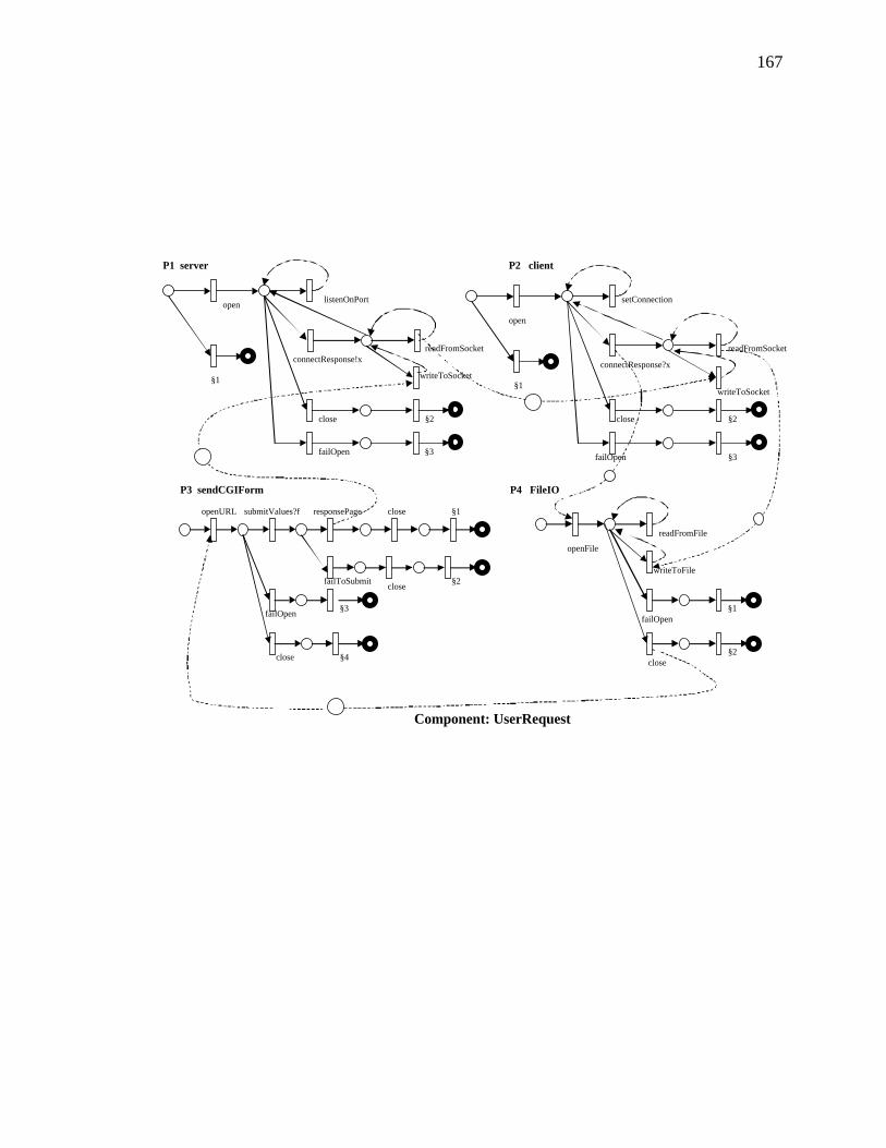
167
open
§1
listenOnPort
connectResponse!xreadFromSocket
writeToSocket
§2close
failOpen §3
open
§1
setConnection
connectResponse?x
readFromSocket
writeToSocket
§2
§3
close
failOpen
P2 clientP1 server
openURL
§4
submitValues?f
§2
§1
failToSubmit
responsePage close
§3failOpen
close
P3 sendCGIForm
openFile
§2
readFromFile
§1failOpen
close
writeToFile
Component: UserRequest
P4 FileIO
close
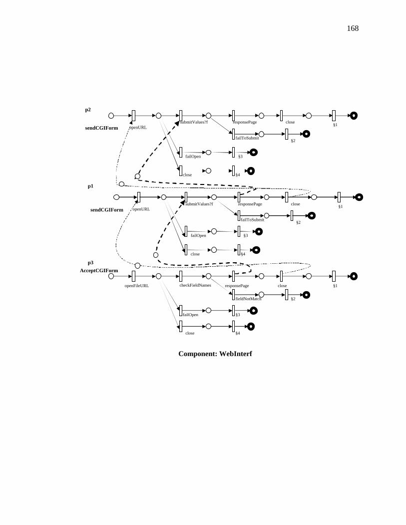
168
Component: WebInterf
openURL
§4
submitValues?f
§2
§1
failToSubmit
responsePage close
§3failOpen
close
sendCGIForm
openURL
§4
submitValues?f
§2
§1
failToSubmit
responsePage close
§3failOpen
close
sendCGIForm
openFileURL
§4
checkFieldNames
§2
§1
fieldNotMatch
responsePage close
§3failOpen
close
AcceptCGIForm
p3
p1
p2

169
REFERENCES
[AAG93] G. Abowd, R. Allen, and D. Garlan. Using Style to Understand Descriptions of SoftwareArchitecture. In Proceedings of the First ACM SIGSOFT Symposium on the Foundations of SoftwareEngineering, pages 9-20, Los Angeles, CA, December 1993.
[Abd-Allah96] A. Abd-Allah, Composing Heterogeneous Software Architectures. DoctoralDissertation, Center for Software Engineering, University of Southern California, Los Angeles, CA90089, August 1996.
[AG94a] R. Allen and D. Garlan. Formal Connectors. Technical Report, CMU-CS-94-115,Carnegie Mellon University, March 1994.
[AG94b] R. Allen and D. Garlan. Formalizing Architectural Connection. In Proceedings of theSixteenth International Conference on Software Engineering, pages 71-80, Sorrento, Italy, May1994.
[AG94c] R. Allen and D. Garlan. Beyond Definition/Use: Architectural Interconnection. InProceedings of the Workshop on Interface Definition Languages, Vol 29, J. M. Wing(Ed.), ACMSIGPLAN Notices, Portland, Oregon, January 1994.
[AG96] R. Allen and D. Garlan. A Case Study in Architectural Modeling: The AEGIS System. InProceedings of the Eighth International Conference on Software Specification and Design (IWSSD-8), pages 6-15, Paderborn, Germany, March 1996.
[AGI98] R. Allen, D. Garlan, and J. Ivers, Formal Modeling and Analysis of the HLA ComponentIntegration Standards. In Proceedings of the Sixth International Symposium on the Foundations ofSoftware Engineering (FSE-6), Lake Buena Vista, Florida, November 1998.
[All96] R. Allen. HLA: A Standards Effort as Architectural Style. In A. L. Wolf, ed., In Proceedingsof the Second International Software Architecture Workshop (ISAW-2), pages 130-133, SanFrancisco, CA, October 1996.

170
[All97] R. Allen. A Formal Approach to Software Architecture. Ph.D. Thesis, Carnegie MellonUniversity, Technical Report Number: CMU-CS-97-144, May 1997.
[ATT93] Software Architecture Validation. AT&T Technical Journal Current, 1993.
[Bei90] B. Beizer. Software Testing Techniques. Van Nostrand Reinhold, Inc, New York, NY, 2ndedition, 1990. ISBN 0-442-20672-0.
[BIMR97] A. Bertolino, P. Inverardi, H. Muccini, and A. Rosetti, An Approach to Integration TestingBased on Architectural Descriptions. In Proceedings of the Third IEEE International Conference onEngineering of Complex Computer Systems (ICECCS97), pages 77-84, Como, Italy, September 1997.
[Clark00] L. A. Clarke. Improve Architectural Description Languages to Support Analysis Better.Workshop on Evaluating Software Architectural Solutions 2000 (WESAS), http://www.isr.uci.edu/events/wesas2000/, Irvine, CA, May 2000.
[Cle96a] P. C. Clements. A Survey of Architecture Description Languages. In Proceedings of theEighth International Workshop on Software Specification and Design, Paderborn, Germany,March 1996.
[DSSA92] LTC E. Mettala and M. H. Graham. The Domain-Specific Software Architecture Program,Technical Report, Carnegie Mellon Software Engineering Institute, CMU/SEI-92-SR-009, 1992.
[EG99] A. Egyed and C. Gacek. Automatically Detecting Mismatches during Component-Based andModel-Based Development, In Proceedings of the 14th IEEE International Conference on AutomatedSoftware Engineering, pages 191-198. Cocoa Beach, Florida, October 1999
[FW88] P. G. Frankl and E. J. Weyuker, An Applicable Family of Data Flow Testing Criteria, IEEETransactions on Software Engineering, 14(10), 1483-1498, October 1988.
[GACB95] C. Gacek, A. Abd-Allah, B. K. Clark and B. Boehm. On the Definition of SoftwareSystem Architecture. In Proceedings of the First International Workshop on Architectures forSoftware Systems - In Cooperation with the 17th International Conference on Software Engineering.D. Garlan (ed.), pages 85-95, Seattle, April 1995, .
[GACEK98] C. Gacek. Detecting Architectural Mismatches During Systems Composition. DoctoralDissertation, Center for Software Engineering, University of Southern California, Los Angeles, CA90089, December 1998.

171
[GACEK99] C. Gacek and B. Boehm. Composing Components: How Does One Detect PotentialArchitectural Mismatches? In Proceedings of the OMG-DARPA-MCC Workshop on CompositionalSoftware Architectures, January 1998
[GAO94] D. Garlan, R. Allen, and J. Ockerbloom. Exploiting Style in Architectural DesignEnvironments. In Proceedings of SIGSOFT'94: Foundations of Software Engineering, pages 175-188,New Orleans, Louisiana, USA, December 1994.
[GAO95a] D. Garlan, R. Allen, and J. Ockerbloom. Architectural Mismatch or Why it's Hard to BuildSystems Out of Existing Parts. In Proceedings of the 17th International Conference on SoftwareEngineering, pages 179--185. Association for Computer Machinery, April 1995.
[GAO95b] D. Garlan, R. Allen, and J. Ockerbloom. Architectural Mismatch: Why Reuse is So Hard.IEEE Software, 12(6): pages 17--26, November 1995.
[GMW95] D. Garlan, R. Monroe, and D. Wile. ACME: An Architectural Interconnection Language.Technical Report, CMU-CS-95-219, Carnegie Mellon University, November 1995.
[GMW97] D. Garlan, R. Monroe, and D. Wile. ACME: An Architecture Description InterchangeLanguage. In Proceedings of IBM CASCON'97, Toronto, Canada, January 1997.
[GR84] U. Goltz and W. Reisig. CSP-Programs As Nets With Individual Tokens. Lecture Notes inComputer Sciences, Vol 188, pages169-196, 1984.
[GS93] D. Garlan and M. Shaw. An Introduction to Software Architecture: Advances in SoftwareEngineering and Knowledge Engineering, Volume I. World Scientific Publishing, 1993.
[Hoa85] C. A. R. Hoare. Communicating Sequential Processes. Prentice Hall, 1985.
[HR94] M. J. Harrold and G. Rothermel. Performing Data Flow Testing on Classes. Symposium onFoundations of Software Engineering (ACM SIGSOFT 94), pages 154-163, December 1994.
[IW95] P. Inverardi and A. L. Wolf. Formal Specification and Analysis of Software ArchitecturesUsing the Chemical Abstract Machine Model. IEEE Transactions on Software Engineering,vol.21, no.4, pages 373-386, April 1995.

172
[Jensen97] K. Jensen: Coloured Petri Nets. Basic Concepts, Analysis Methods and Practical Use.Volume 1, Basic Concepts. Monographs in Theoretical Computer Science, Springer-Verlag, 2ndcorrected printing 1997.
[Jin94] Z. Jin. Deadlock and Trap Analysis in Petri Nets. MS Thesis, Computer Science Department,George Mason University, Fairfax, VA. 1994.
[JJ2000] Z. Jin, A. J. Offutt, A. Abdurazik, and E. L.White. Analyzing Software ArchitectureDescriptions to Generate System-level Tests. Workshop on Evaluating Software ArchitecturalSolutions 2000 (WESAS), http://www.isr.uci.edu/events/wesas2000/, Irvine, CA, May 2000.
[JO 98] Z. Jin and A. J. Offutt. Coupling-based Criteria for Integration Testing. Software Testing,Verification, and Reliability, 8(3), pages 133-154, September 1998.
[KBA+94] R. Kazman, L. Bass, G. Abowd, and M. Webb. SAAM:A Method for Analyzing theProperties of Software Architectures. In Proceedings of the Sixteenth International Conference onSoftware Engineering, May 1994, pages 81-90, 1993.
[KC94] P. Kogut and P. Clements. Features of Architecture Description Languages. Draft of aCMU/SEI Technical Report, December 1994.
[KC95] P. Kogut and P. Clements. Feature Analysis of Architecture Description Languages. InProceedings of the Software Technology Conference (STC'95), Salt Lake City, April 1995.
[LKA+95] D. C. Luckham, J. J. Kenney, L. M. Augustin, J. Vera, D. Bryan, and W. Mann.Specification and Analysis of System Architecture Using Rapide. IEEE Transactions on SoftwareEngineering, Vol. 21, no.4, pages 336-355, April 1995.
[LV95] D. C. Luckham and J. Vera. An Event-Based Architecture Definition Language. IEEETransactions on Software Engineering, Vol. 21, no.9, pages 717-734, September 1995.
[LVB+93] D. C. Luckham, J. Vera, D. Bryan, L. Augustin, and F. Belz. Partial Orderings of EventSets and Their Application to Prototyping Concurrent, Timed Systems. The Journal of Systemsand Software, Vol. 21, no.3, pages 253-265, June 1993.
[LVM00] D. C. Luckham, J. Vera, and S. Meldal. Key Concepts in Architecture DefinitionLanguages. Foundations of Component-Based Systems. G. T. Leavens and L. Sitaraman (Ed.),Cambridge University Press, pages 23-45, New York, 2000.

173
[Med96] N. Medvidovic. ADLs and Dynamic Architecture Changes. In A. L. Wolf, ed., Proceedingsof the Second International Software Architecture Workshop (ISAW-2), pages 24-27, San Francisco,CA, October 1996.
[Med97] N. Medvidovic. A Classification and Comparison Framework for Software ArchitectureDescription Languages. Technical Report, UCI-ICS-97-02, University of California, Irvine,January 1997.
[MOT96a] N. Medvidovic, P. Oreizy, and R. N. Taylor. Reuse of Off-the-Shelf Components in C2-Style Architectures. In Proceedings of the 1997 Symposium on Software Reusability(SSR'97),pages 190-198, Boston, MA, May 17-19, 1997. Also in Proceedings of the 1997 InternationalConference on Software Engineering (ICSE'97), pages 692-700, Boston, MA, May 17-23, 1997.
[MORT96b] N. Medvidovic, P. Oreizy, J. E. Robbins, and R. N. Taylor. Using Object-Orientedtyping to support architectural design in the C2 style. In Proceedings of the ACM SIGSOFT'96:Fourth Symposium on the Foundations of Software Engineering (FSE4), pages 24-32, SanFrancisco,CA, October 1996.
[MPW92] R. Milner, J. Parrow, and D. Walker. A Calculus of Mobile Processes, Parts I and II.Volume 100 of the Journal of Information and Computation, pages 1-40 and 41-77, 1992.
[MQ94] M. Moriconi and X. Qian. Correctness and Composition of Software Architectures. InProceedings of the Second ACM SIGSOFT Symposium on the Foundations of Software Engineering,ACM SIGSOFT Software Engineering Notes, 19(5):164-174. December 1994.
[MQR95] M. Moriconi, X. Qian, and R. A. Riemenschneider. Correct Architecture Refinement.IEEE Transactions on Software Engineering, Vol. 21, no.4, pages 356-372, April 1995.
[MT97] N. Medvidovic and R. N. Taylor. Reuse of Off-the-Shelf in C2 Style Architectures InProceedings of the 19 th International Conference on Software Engineering (ICSE 97). pages 692-700,Springer, Berlin - Heidelberg - New York, May 1997.
[MTW96] N. Medvidovic, R. N. Taylor, and E. J. Whitehead, Jr. Formal Modeling ofSoftware Architectures at Multiple Levels of Abstraction. In Proceedings of the CaliforniaSoftware Symposium 1996, pages 28-40, Los Angeles, CA, April 1996.

174
[OA99] A. J. Offutt and A. Abdurazik. Generating Tests from UML Specifications. In Proceedings ofthe Second International Conference on the Unified Modeling Language (UML99), Fort Collins, CO,October 1999.
[OJP99] A. J. Offutt, Z. Jin, and J. Pan. The Dynamic Domain Reduction Procedure for Test DataGeneration. The Journal of Software Practice and Experience. Vol.29, no. 2, pages 167-193,Feburary 1999.
[OYS99] A. J. Offutt, Y. Xiong and S. Liu. Criteria for Generating Specification-based Tests. FifthIEEE International Conference on Engineering of Complex Computer Systems (ICECCS '99), LasVegas, NV, October 1999.
[Perterson81] Peterson, J. L. Petri Net Theory and the Modeling of Systems, Prentice Hall,Englewood Cliffs, NJ. 1981.
[PN86] R. Prieto-Diaz and J. M. Neighbors. Module Interconnection Languages. The Journal ofSystems and Software, Vol. 6, no. 4, pages 307-334, November 1986.
[Pur94] J. Purtilo. The Polylith Software Bus. ACM Transactions on Programming Languages andSystems. Vol 16(1). pages 151-174, January 1994.
[ROS98] A. W. Roscoe. The Theory and Practice of Concurrency. Prentice Hall, 1998.
[Rosen00] D. S. Rosenblum. Challenges in Exploiting Architectural Models for Software Testing.Workshop on Evaluating Software Architectural Solutions 2000 (WESAS), http:// www.isr.uci.edu/events/wesas2000/, Irvine, CA, May 2000.
[Rosen97] D. S. Rosenblum. Adequate Testing of Component-Based Testing. Technical Report 97-34, Dept. of Information and Computer Science, University of California, Irvine, CA. August 1997.
[RR96] J. E. Robbins and D. Redmiles. Software Architecture Design From the Perspective ofHuman Cognitive Needs. In Proceedings of the California Software Symposium (CSS'96), LosAngeles, CA, USA, April 1996.
[RT86] G. Rozenberg, and P. S. Thiagarajan. Petri Nets: Basic Notions, Structure and Behavior.Lecture Notes in Computer Science. Vol. 224, pages 585-668 Springer-Verlag, Berlin, Germany.1986.

175
[RW96] D. J. Richardson and A. L. Wolf. Software Testing at the Architectural Level. InProceedings of the Second International Software Architecture Workshop (ISAW-2), San Francisco,California, pages 68-71. October 1996
[SC93] P. Stocks and D. Carrington. Test Templates: A Specification-Based Testing Framework. InProceedings of the 15th International Conference on Software Engineering, pages 405-414,Baltimore, MD, May 1993.
[SDK+95] M. Shaw, R. DeLine, D. V. Klein, T. L. Ross, D. M. Young, and G. Zelesnik. Abstractionsfor Software Architecture and Tools to Support Them. IEEE Transactions on Software Engineering,pages 314-335, April 1995.
[SG94] M. Shaw and D. Garlan. Characteristics of Higher-Level Languages for SoftwareArchitecture. Technical Report, CMU-CS-94-210, Carnegie Mellon University, December 1994.
[SG95] M. Shaw and D. Garlan. Formulations and Formalisms in Software Architecture.Springer-Verlag Lecture Notes in Computer Science, Vol. 1000, pages 307-320, 1995.
[SG96] M. Shaw and D. Garlan. Software Architecture: Perspectives on an Emerging Discipline,Prentice Hall, 1996.
[Spi89] J. M. Spivey. The Z notation: A Reference Manual. Prentice Hall, New York, 1989.
[SRW97] J. A. Stafford, D. J. Richardson, and A. L. Wolf. Chaining: A Software ArchitectureDependence Analysis Technique. Technical Report CU-CS-845-97, University of Colorado,September 1997.
[SRW98] J. A. Stafford, D. J. Richardson, and A. L. Wolf. Aladdin: A Tool for Architecture-levelDependence Analysis of Software Systems. University of Colorado Technical Report, CU-CS-858-98, 1998.
[STARS93] Software Technology for Adaptable, Reliable Systems [STARS]. ConceptualFramework for Reuse Processes (CFRP), Volume I: Definition, Version 3.0, STARS-VC-A018/001/00, 25 October, 1993.
[Tra93] W. Tracz. LILEANNA: A Parameterized Programming Language. In Proceedings of theSecond International Workshop on Software Reuse, pages 66-78, Lucca, Italy, March 1993.

176
[Ves93] S. Vestal. A Cursory Overview and Comparison of Four Architecture DescriptionLanguages. Technical Report, Honeywell Technology Center, February 1993.
[Ves96] S. Vestal. MetaH Programmer's Manual, Version 1.09. Technical Report, HoneywellTechnology Center, April 1996.
[Web] www-ast.tds-gn.Imco.com/arch/ Software Architecture Technology Guide
[Wey86] E. J. Weyuker. Axiomatizing Software Test Data Adequacy. IEEE Transactions onSoftware Engineering, Vol. 12, no. 12, pages 1128-1138, December 1986.
[Wolf96] A. L. Wolf, editor. In Proceedings of the Second International Software ArchitectureWorkshop (ISAW-2), San Francisco, CA, October 1996.
[Wolf97] A. L. Wolf. In Proceedings of the Second International Software Architecture Workshop(ISAW-2). ACM SIGSOFT Software Engineering Notes, pages 42-56, January 1997.
[Wrighttool] http://www.cs.cmu.edu/afs/cs/project/able/ftp/Wright-tutorial.ps
[You96] E. Yourdon. Software Quality Assurance in the 1990s. Technical report, HoneywellTechnollogy Center, April 1996.
[ZHM97] H. Zhu, P. A. V. Hall, and H. R. J. May. Software Unit Test Coverage and Adequacy. ACMComputing Surveys, 29(4), pages 366-427, December 1997.