This content has been downloaded from IOPscience. Please scroll down to see the full text.

Download details:

IP Address: 155.98.164.36

This content was downloaded on 30/04/2015 at 15:47

Please note that terms and conditions apply.

A slice-by-slice blurring model and kernel evaluation using the Klein-Nishina formula for 3D

scatter compensation in parallel and converging beam SPECT

View the table of contents for this issue, or go to the journal homepage for more

2000 Phys. Med. Biol. 45 1275

(http://iopscience.iop.org/0031-9155/45/5/314)

Home Search Collections Journals About Contact us My IOPscience

Phys. Med. Biol. 45 (2000) 1275–1307. Printed in the UK PII: S0031-9155(00)07327-9

A slice-by-slice blurring model and kernel evaluation using theKlein–Nishina formula for 3D scatter compensation in paralleland converging beam SPECT

Chuanyong Bai, Gengsheng L Zeng and Grant T GullbergDepartment of Radiology, University of Utah, 729 Arapeen Drive, Salt Lake City,Utah 84108-1218, USA

E-mail: bai@pet.upmc.edu

Received 1 September 1999, in final form 21 February 2000

Abstract. Converging collimation increases the geometric efficiency for imaging small organs,such as the heart, but also increases the difficulty of correcting for the physical effects of attenuation,geometric response and scatter in SPECT. In this paper, 3D first-order Compton scatter in non-uniform scattering media is modelled by using an efficient slice-by-slice incremental blurringtechnique in both parallel and converging beam SPECT. The scatter projections are generatedby first forming an effective scatter source image (ESSI), then forward-projecting the ESSI. TheCompton scatter cross section described by the Klein–Nishina formula is used to obtain spatialscatter response functions (SSRFs) of scattering slices which are parallel to the detector surface.Two SSRFs of neighbouring scattering slices are used to compute two small orthogonal 1D blurringkernels used for the incremental blurring from the slice which is further from the detector surface tothe slice which is closer to the detector surface. First-order Compton scatter point response functions(SPRFs) obtained using the proposed model agree well with those of Monte Carlo (MC) simulationsfor both parallel and fan beam SPECT. Image reconstruction in fan beam SPECT MC simulationstudies shows increased left ventricle myocardium-to-chamber contrast (LV contrast) and slightlyimproved image resolution when performing scatter compensation using the proposed model.Physical torso phantom fan beam SPECT experiments show increased myocardial uniformity andimage resolution as well as increased LV contrast. The proposed method efficiently models the 3Dfirst-order Compton scatter effect in parallel and converging beam SPECT.

1. Introduction

In single photon emission computed tomography (SPECT), a large number of scatteredphotons are detected because of the wide energy window used (typically 15–20%). Imagereconstruction without scatter compensation has degraded image quality (i.e. reduced contrastand resolution) and biased quantitation (Jaszczak et al 1985). Intensive efforts have been madeto compensate for the scatter effect in SPECT in order to improve the quantitative and qualitativeaccuracy of the reconstructed images. While these efforts have improved the reconstructedimages, none of these methods can perform fast and accurate scatter compensation in non-uniform scattering objects in converging beam SPECT.

A class of widely used and widely studied scatter compensation methods is based onthe estimation of the scatter component in the photo-peak projection data and subsequentsubtraction or deconvolution of the scatter contribution from the measured projection data.Many of the subtraction-based scatter compensation methods use multiple energy window

0031-9155/00/051275+33$30.00 © 2000 IOP Publishing Ltd 1275

1276 C Bai et al

acquisition methods (Jaszczak et al 1984, 1985, Lowry and Cooper 1987, Koral et al 1988,1990, Ogawa et al 1991, Gagnon et al 1989, Halama et al 1988, DeVito et al 1989, Hamilland Devito 1989, King et al 1992, Frey et al 1992) to estimate the scatter contribution. Theestimated scatter component can be subtracted from the photo-peak projection data to obtainthe scatter-compensated projection data. Scatter compensation methods in this class are fastand simple, but increase the noise in the reconstructed images. Alternatively, the deconvolutionmethods use kernels that are obtained from physical measurements using a Gamma camera(Axelsson et al 1984, Floyd et al 1985a, Msaki et al 1987, 1989, Meikle et al 1994). Usually,the scatter component is deconvolved from the projection data before reconstruction.

Another class of scatter compensation methods is based on modelling scatter effects (thescatter response function) in the projector–backprojector (transition matrix) used in iterativereconstruction methods (Floyd et al 1985b, Frey et al 1993, Frey and Tsui 1993, Beekmanet al 1993, 1996, Welch et al 1995). The techniques for modelling the non-uniform attenuationeffect (Tsui et al 1989), the detector response effect (Tsui et al 1988, 1994, Formiconi et al1989, Zeng et al 1991, Gilland et al 1994) and the scatter effect (Floyd et al 1985b, 1986, 1987,Veklerov et al 1988, Frey and Tsui 1990, 1993, 1994, 1996, Bowsher and Floyd 1991, Freyet al 1992, 1993, Beekman et al 1993, 1994, 1995, 1996, 1997, Riauka and Gortel 1994, Caoet al 1994, Meikle et al 1994, Walrand et al 1994, Ju et al 1995, Welch et al 1995, Kadrmaset al 1996, 1997, 1998, Hutton et al 1996, Riauka et al 1996, Wells et al 1997, Hutton 1997) ina realistic projector–backprojector (transition matrix) may lead to accurate compensation forthese image-degrading effects in SPECT image reconstruction. We call this class of methodsreconstruction-based scatter compensation methods.

The accuracy of a reconstruction-based scatter compensation method is dependent uponthe accuracy of the scatter model used. A complicating factor in modelling scatter is that thescatter response is generally different for every point in the object to be imaged.

Several techniques have been developed for calculating the transition matrix (scattermodel) in the projector–backprojector so that it is a function of the anatomy being imaged.One technique computes the transition matrix using Monte Carlo (MC) simulations (Floydet al 1985b, 1986, 1987, Veklerov et al 1988, Frey and Tsui 1990, Bowsher and Floyd 1991).This approach requires large data storage capacities and long computation times. A secondtechnique actually makes physical measurements (Beekman et al 1994, Walrand et al 1994). Athird technique is referred to as slab derived scatter estimation. This technique first calculatesand stores the scatter response tables for a point source behind slabs of a range of thicknesses,and tunes the model to various object shapes including non-uniform attenuators (Frey et al1993, Frey and Tsui 1993, Beekman et al 1993, 1996, 1997, Beekman and Viergever 1995).A table occupying a few megabytes of memory is sufficient for representing this scatter modelfor fully 3D reconstruction. A fourth method is based upon the integration of the Klein–Nishina formula in non-uniform media (Riauka and Gortel 1994, Cao et al 1994, Riaukaet al 1996, Wells et al 1998). Like Monte Carlo techniques this technique requires large datastorage capacities and long computation times. A fifth method uses a variable attenuationmap to model first-order scatter at each image site by projecting and backprojecting along allpossible lines of scatter using a ray-driven projector–backprojector (Welch et al 1995, Welchand Gullberg 1996, 1997, Laurette et al 1999).

Reconstruction-based scatter compensation methods (Floyd et al 1986, Frey et al 1993,Beekman et al 1996, Kadrmas et al 1998) have been shown to result in images withless variance when compared with subtraction-based scatter compensation methods (Freyet al 1992, Beekman et al 1997). The main disadvantage of reconstruction-based scattercompensation is that the scatter models tend to be very computationally intensive. Recentadvances in fast implementations of reconstruction-based methods such as using coarse-grid

Blurring model and kernel evaluation for SPECT 1277

modelling approaches (Kadrmas et al 1998), unmatched projector–backprojector pairs (Zengand Gullberg 1996, 1997, 2000, Welch and Gullberg 1996, 1997, Kamphuis et al 1998)and accelerated iterative algorithms (Hudson and Larkin 1994, Byrne 1996), can make thereconstruction time for reconstruction-based scatter correction techniques more reasonable.

The method presented in this paper is based on use of an incremental blurring techniqueto model the scatter in the projector. The incremental blurring technique was first developedto model the geometric detector response in the projector–backprojector pair (McCarthy andMiller 1991, Wallis et al 1996, Di Bella et al 1996, Zeng et al 1998). In this work, theincremental blurring approach is used to decrease the computational requirement for modellingscatter.

Frey and Tsui (1996) proposed an effective scatter source estimation (ESSE) scattermodel to model 3D scatter response in SPECT. This technique produces an effective scattersource which is used to generate the estimated scatter projection by forward-projecting theeffective scatter source, using a projector that models both attenuation and geometric detectorresponse effects. The projector used for forward-projecting the effective scatter source canbe implemented using the incremental blurring technique for modelling the non-uniformattenuation and depth-dependent geometric point response. The activity image is convolvedwith several kernels to obtain the effective scatter source. The effective scatter source kerneland the relative scatter attenuation coefficient kernel used for the convolutions are generatedby Monte Carlo simulations and are assumed to be independent of the source position. Thetechnique models the non-uniform attenuation effect from the scattering point to the detector,but does not model the non-uniform attenuation from the source to the scattering point. Themethod does not have the capacity to provide an exact scatter estimate when extended toconverging beam collimation.

Zeng et al (1999) were the first to propose using a slice-by-slice blurring technique tomodel 3D first-order Compton scatter in SPECT for parallel beam geometry, and Bai et al(1998b) extended the technique to model 3D first-order Compton scatter in SPECT for fan-beam geometry. The scatter projection was generated by first forming an effective scattersource image (similar to the effective scatter source in Frey and Tsui’s (1996) model) usinga slice-by-slice blurring model, then forward-projecting the effective scatter source imageusing a slice-by-slice blurring model which modelled the non-uniform attenuation effect andthe depth-dependent geometric detector response effect. The small blurring kernels wereobtained by recursively changing a parameter which was used to calculate the kernels untilthe generated first-order Compton scatter projection was best matched to the Monte Carlogenerated first-order Compton scatter projection. The kernels were stationary, and were usedto model first-order Compton scatter for Compton scatter compensation in SPECT imaging.

The incremental blurring method proposed in this paper to model first-order Comptonscatter is based on the Klein–Nishina formula. The key to this method is to transform theKlein–Nishina formula so that the scatter angle is expressed in terms of the spatial coordinates,i.e. the positions of the point source, the scattering point and the detection point, as well asthe focal length of the converging beam collimator. An effective scatter source image (ESSI)can be obtained using a slice-by-slice blurring model, with the blurring kernels approximatedfrom the transformed Klein–Nishina formula. Scatter projections can be obtained by forward-projecting the ESSI using a projector, which models non-uniform attenuation and geometricdetector response effects.

In section 2 the Klein–Nishina formula is introduced and the slice-by-slice blurring modelis derived. In sections 3 and 4 the model is evaluated by comparing the scatter point responsefunctions (SPRFs) and the scatter response of a distributed source generated using the proposedmodel with those generated from Monte Carlo (MC) simulations. The model is also evaluated

1278 C Bai et al

by comparing the measured total point response of a fan-beam SPECT system with thatgenerated using the proposed model. Fan-beam SPECT reconstructions are used to showthe effect of performing fully 3D scatter compensation using the proposed model. Section 5includes some discussion and, finally, in section 6, conclusions are drawn from the previousresults and discussions.

2. Theory

Compton scatter is an important interaction mechanism when high-energy photons interactwith materials. This scatter is accompanied by energy transfer to the material. Within thediagnostic energy range of nuclear medicine, the linear attenuation coefficients of body tissuesare essentially composed of contributions from Compton scatter and photoelectric absorption(Alvarez and Macovski 1976, Phelps et al 1975). We propose in this paper the use of a slice-by-slice blurring model for first-order Compton scatter with the justification that 80% to 90%of the scattered events detected in an 18% 99mTc emission window are caused by first-orderCompton scatter (Floyd et al 1984).

2.1. Modelling first-order Compton scatter in SPECT

2.1.1. The Klein–Nishina formula. The photon energy and scatter-angle-dependent Comptonscatter differential cross section of an electron is expressed by the Klein–Nishina formula (Kleinand Nishina 1928, Johns and Cunningham 1974). In SPECT, we consider the scatter effect ofa voxel in the scattering object to be given by the differential cross-section dσ/d�, defined bythe equation

dσ

d�= R0

((1 + cos2 θ)[1 + α(1− cos θ)] + α2(1− cos θ)2

[1 + α(1− cos θ)]3

)= R0F(θ,E) (1)

where R0 is a scatter factor dependent upon the composition of the scattering medium and thevolume of the voxel. That is to say, R0 depends upon the total number of free and looselybound electrons in the voxel, θ is the scatter angle, α is the ratio of the energyE of the incidentphoton to the energy of an electron at rest (511 keV) and F(θ,E) is the expression in the largebrackets of equation (1). The equation for the differential cross section can be simplified asthe product ofR0 and the factor F(θ,E) (which is only dependent upon the photon energy andscatter angle). For non-uniform scattering objects, R0 can be different from voxel to voxel.

2.1.2. Scatter point response function (SPRF). The generation of a first-order Comptonscatter point response function (SPRF) at the detector, for a point source SS (figure 1), can bedecomposed into four consecutive steps:

(a) Step 1. Photons propagate from the point source to a scattering voxel SC. At the sametime the intensity is attenuated by a factor of ASS→SC, which is the total attenuation effectfrom the point source to the scattering voxel.

(b) Step 2. Photons are scattered at SC with the scatter probability described by the Klein–Nishina formula in equation (1): R0F(θ,E). The effective scatter at the point SC for thepoint source at SS is

E(SC,SS) = ISSASS→SCR0F(θ,E) (2)

where ISS is the point source intensity.

Blurring model and kernel evaluation for SPECT 1279

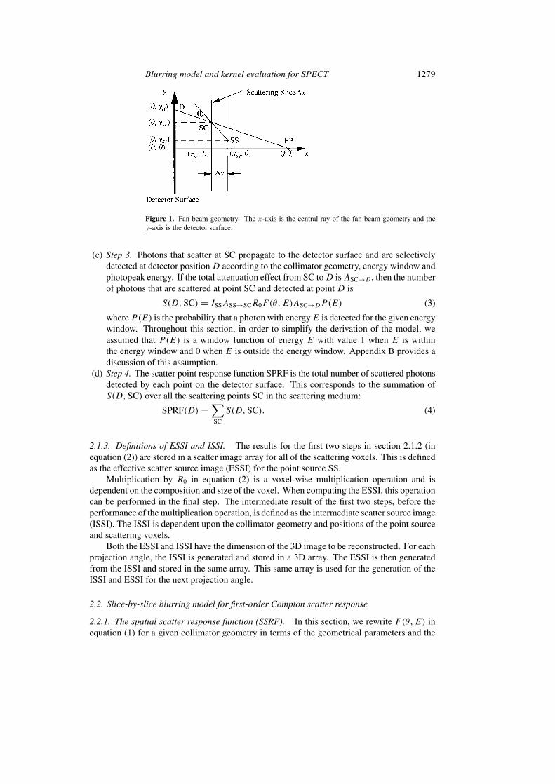
Figure 1. Fan beam geometry. The x-axis is the central ray of the fan beam geometry and they-axis is the detector surface.

(c) Step 3. Photons that scatter at SC propagate to the detector surface and are selectivelydetected at detector positionD according to the collimator geometry, energy window andphotopeak energy. If the total attenuation effect from SC toD isASC→D , then the numberof photons that are scattered at point SC and detected at point D is

S(D,SC) = ISSASS→SCR0F(θ,E)ASC→DP (E) (3)

where P(E) is the probability that a photon with energyE is detected for the given energywindow. Throughout this section, in order to simplify the derivation of the model, weassumed that P(E) is a window function of energy E with value 1 when E is withinthe energy window and 0 when E is outside the energy window. Appendix B provides adiscussion of this assumption.

(d) Step 4. The scatter point response function SPRF is the total number of scattered photonsdetected by each point on the detector surface. This corresponds to the summation ofS(D,SC) over all the scattering points SC in the scattering medium:

SPRF(D) =∑SC

S(D,SC). (4)

2.1.3. Definitions of ESSI and ISSI. The results for the first two steps in section 2.1.2 (inequation (2)) are stored in a scatter image array for all of the scattering voxels. This is definedas the effective scatter source image (ESSI) for the point source SS.

Multiplication by R0 in equation (2) is a voxel-wise multiplication operation and isdependent on the composition and size of the voxel. When computing the ESSI, this operationcan be performed in the final step. The intermediate result of the first two steps, before theperformance of the multiplication operation, is defined as the intermediate scatter source image(ISSI). The ISSI is dependent upon the collimator geometry and positions of the point sourceand scattering voxels.

Both the ESSI and ISSI have the dimension of the 3D image to be reconstructed. For eachprojection angle, the ISSI is generated and stored in a 3D array. The ESSI is then generatedfrom the ISSI and stored in the same array. This same array is used for the generation of theISSI and ESSI for the next projection angle.

2.2. Slice-by-slice blurring model for first-order Compton scatter response

2.2.1. The spatial scatter response function (SSRF). In this section, we rewrite F(θ,E) inequation (1) for a given collimator geometry in terms of the geometrical parameters and the

1280 C Bai et al

positions of the point source, the scattering point and the detection point. Fan beam geometryis used to keep our analysis general.

Figure 1 illustrates a fan beam geometry positioned in the fan direction. Photons emittedfrom a point source SS(xSS, ySS) are scattered by a scattering point SC(xSC, ySC) on a scatteringslice which is parallel to the detector surface and closer to the detector surface than the pointsource. Some of the scattered photons are detected by the camera at pointD(0, yd). The y-axisis on the detector surface and the x-axis is along the central ray of the fan beam geometry. Thefocal point is at FP(f, 0), where f is the focal length. The distance in the x-direction from thescattering point to the point surface is �x. A scattering slice at a distance �x closer to thedetector surface than the point source will be denoted by ‘the scattering slice �x’ throughoutthe rest of this paper. The unit used for distance is ‘bin’, which is the projection bin size.

The scatter angle at SC(xSC, ySC) can be expressed in terms of f , xSS, ySS, yd , and�x as:

θ = arctan

[(yd(f − xSS +�x)

f− ySS

)(�x)−1

]− arctan(yd/f ). (5)

Note that the coordinates (xSC, ySC) of the scattering point can be determined from f ,xSS, ySS, yd and �x. As a special case for the parallel geometry, the scatter angle isθ = arctan[(yd − ySS)/(�x)].

Substituting equation (5), as well as f and E, into F(θ,E) in equation (1), for a givenpoint source position, allows one to examine the behaviour of F as a function of yd and �xin both the fan direction and the parallel direction. To do this we will define a new functionGfan(yd,�x) = F(θ,E) for a given energy in the plane of the fan beam direction. Thisessentially provides a 1D spatial scatter response function (SSRF) for first-order Comptonscatter for a scattering slice at a distance �x from the point source. By the same token, wedefine Gpar(zd,�x) = F(θ,E) in the plane of the parallel beam direction, where zd is thecoordinate in the z direction (parallel beam direction).

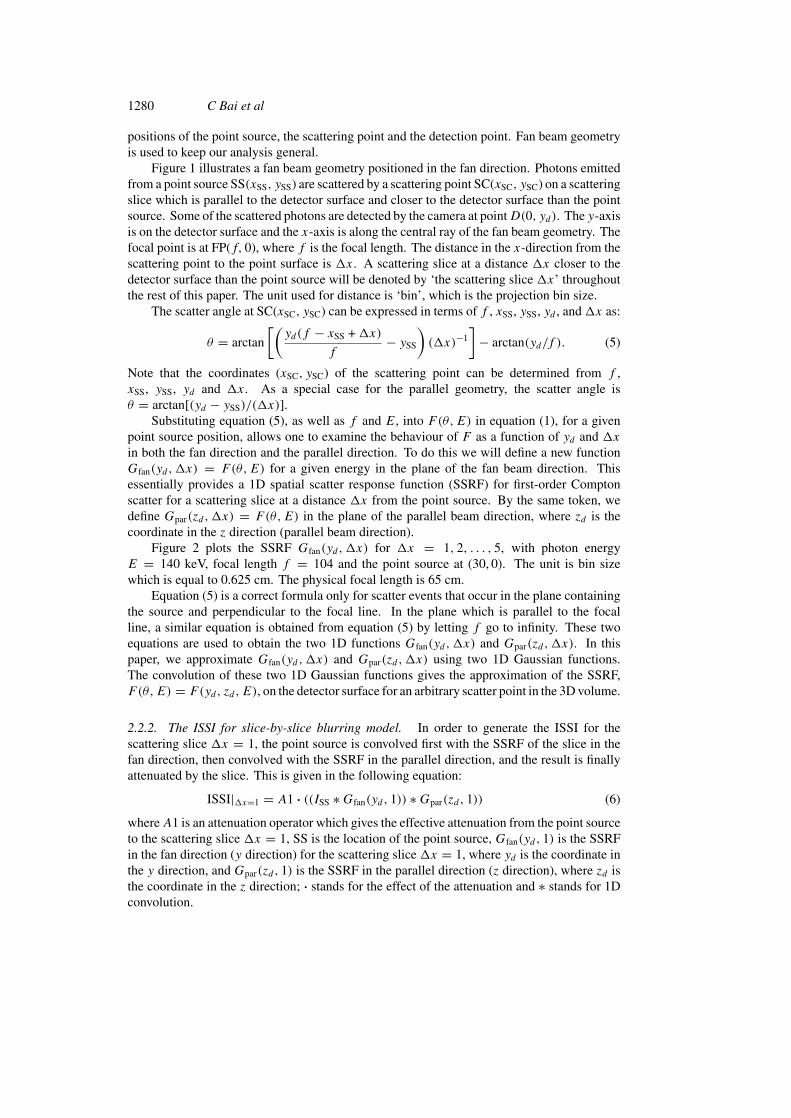
Figure 2 plots the SSRF Gfan(yd,�x) for �x = 1, 2, . . . , 5, with photon energyE = 140 keV, focal length f = 104 and the point source at (30, 0). The unit is bin sizewhich is equal to 0.625 cm. The physical focal length is 65 cm.

Equation (5) is a correct formula only for scatter events that occur in the plane containingthe source and perpendicular to the focal line. In the plane which is parallel to the focalline, a similar equation is obtained from equation (5) by letting f go to infinity. These twoequations are used to obtain the two 1D functions Gfan(yd,�x) and Gpar(zd,�x). In thispaper, we approximate Gfan(yd,�x) and Gpar(zd,�x) using two 1D Gaussian functions.The convolution of these two 1D Gaussian functions gives the approximation of the SSRF,F(θ,E) = F(yd, zd, E), on the detector surface for an arbitrary scatter point in the 3D volume.

2.2.2. The ISSI for slice-by-slice blurring model. In order to generate the ISSI for thescattering slice �x = 1, the point source is convolved first with the SSRF of the slice in thefan direction, then convolved with the SSRF in the parallel direction, and the result is finallyattenuated by the slice. This is given in the following equation:

ISSI|�x=1 = A1 · ((ISS ∗Gfan(yd, 1)) ∗Gpar(zd, 1)) (6)

whereA1 is an attenuation operator which gives the effective attenuation from the point sourceto the scattering slice �x = 1, SS is the location of the point source, Gfan(yd, 1) is the SSRFin the fan direction (y direction) for the scattering slice�x = 1, where yd is the coordinate inthe y direction, and Gpar(zd, 1) is the SSRF in the parallel direction (z direction), where zd isthe coordinate in the z direction; · stands for the effect of the attenuation and ∗ stands for 1Dconvolution.

Blurring model and kernel evaluation for SPECT 1281

Figure 2. Spatial scatter response function Gfan(yd ,�x) for �x = 1, 2, . . . , 5.

In the same way, the ISSI for the scattering slice �x = 2 can be generated as

ISSI|�x=2 = A12 · A1 · ((ISS ∗Gfan(yd, 2)) ∗Gpar(zd, 2)) (7)

where A12 is an attenuation operator which gives the contribution of the effective attenuationfor the point source from the scattering slice �x = 1 to the scattering slice �x = 2, andA12 · A1 gives the effective attenuation from the point source to the scattering slice �x = 2.

If we compare the spatial scatter response functions for the scattering slices �x = 2 and�x = 1 (for example, the function Gfan(yx,�x) shown in figure 2 for the fan direction), wesee that we can approximate the SSRFs for�x = 2 by convolving the SSRFs for�x = 1 withsmall scatter kernels that model the effect of scatter from slice �x = 1 to �x = 2, as shownin equations (8) and (9):

Gfan(yd, 2) = K12fan(yd) ∗Gfan(yd, 1) (8)

Gpar(zd, 2) = K12par(zd) ∗Gpar(zd, 1) (9)

where K12fan(yd) and K12

par(zd) are the small 1D scatter kernels from �x = 1 to �x = 2 in thefan and parallel directions respectively.

Thus, equation (7) can be rewritten as

ISSI|�x=2 = A12 · ({[A1 · ((ISS ∗Gfan(yd, 1)) ∗Gpar(zd, 1))] ∗K12fan(yd)} ∗K12

par(zd)). (10)

Noticing that the part of equation (10) in square brackets is the same as the right-handside of equation (6), one can rewrite equation (10) as

ISSI|�x=2 = A12 · [(ISSI|�x=1 ∗K12fan(yd)) ∗K12

par(zd)]. (11)

Equation (11) expresses the basic principle behind the proposed slice-by-slice blurringmodel for first-order Compton scatter. Once the ISSI for the scattering slice �x = 1 isgenerated using equation (6), we can compute the ISSIs for each succeeding scattering sliceby performing slice-by-slice blurring using

ISSI|�x=n+1 = An[n + 1] · [(ISSI|�x=n ∗Kn[n+1]fan (yd)) ∗Kn[n+1]

par (zd)] (12)

1282 C Bai et al

where ISSI|�x=n+1 is the ISSI for scattering slice �x = n + 1, ISSI|�x=n is the ISSI forscattering slice�x = n, An[n+ 1] is the effective attenuation from scattering slice�x = n to�x = n + 1, andKn[n+1]

fan (yd) andKn[n+1]par (zd) are the two small 1D kernels for the incremental

blurring from �x = n to �x = n + 1 in the fan and parallel directions respectively.When the slice-by-slice blurring method is used for parallel beam geometry and cone

beam geometry one needs only to substitute the SSRFs and the convolution kernels for theappropriate geometry in each corresponding direction.

2.2.3. Generation of ESSI. Multiplication of the ISSI with the composition-dependent scatterfactor in a voxel by voxel manner gives the effective scatter source image (ESSI), as shown by

ESSI(�x) = R · ISSI(�x) �x = 1, 2, . . . (13)

whereR is the voxel-wise multiplication operator by the composition-dependent scatter factorfor each scattering voxel. In the discrete implementation for the computation of the ESSI, thesolid angle subtended by a voxel on the scattering slice with the origin at the point source andthe solid angle subtended by a bin on the detector surface with the origin at the centre of thescattering voxel must be included in equation (13). A detailed discussion of this is providedin appendix A.

The composition-dependent scatter factor R at scattering voxel i can be obtained fromequation (1) when the attenuation map is given, by integrating both sides of equation (1) over4π solid angle and solving for the factor Ri , which gives

Ri =∫

dσi∫F(θ,E) d�

= µCompi

const(E)∼= µi

const(E)(14)

where∫F(θ,E) d� = const(E) is a function of the energy of the incident photons, and has

a value of 5.70 at energy 140 keV, and∫dσi is the total scatter cross section of the voxel,

which gives the Compton portion µCompi of the linear attenuation coefficient for the voxel. In

this paper we assume that the Compton portion of the total linear attenuation coefficient isapproximately equal to the total linear attenuation coefficient µi for an energy of 140 keV.This approximation is based on the calculation results provided in section 5.3 which are basedupon data given by Alvarez and Macovski (1976) and Phelps et al (1975). The attenuationfor body tissues (with the exception of bones) is more than 98% due to Compton scatter at aphoton energy of 140 keV. Therefore the assumption of a linear attenuation coefficient basedonly upon Compton scatter is acceptable when considering the noise level (several per cent)in SPECT.

2.2.4. Generation of the scatter response for a point source. After the ESSI is computed fora point source, the ESSI image is projected using a projector which models the attenuation andthe depth-dependent geometric detector response to obtain the scatter point response function(SPRF). In the next section, we describe how this is used to calculate the scatter response fora distributed source. Generally speaking, the scattered photons have lower energy than theprimary photons. Therefore, one should consider the increased attenuation of the scatteredphotons when projecting the ESSI. However, the increased attenuation for the scattered photonsis not modelled. We assume that the increase in attenuation is relatively small given thedetection energy window that is used (for example, the linear attenuation coefficient of wateris 0.150 cm−1 at 150 keV and 0.161 cm−1 at 120 keV).

2.2.5. Generation of the scatter response for a distributed source. The scatter response of anextended source distribution can be obtained by superposition of the individual SPRF over the

Blurring model and kernel evaluation for SPECT 1283

extended source distribution. In SPECT image reconstruction, this is done by first computingthe ISSI for the voxel sources (which are treated as point sources) on the first slice (parallel tothe detector surface, furthest from the detector surface) of the source image, then computingthe ISSI for the voxel sources on the second slice of the source image, and so on, until thelast slice of the source image which is closest to the detector surface. The obtained ISSIsare added up to form the total ISSI for the extended source distribution, and equation (13) isused to compute the ESSI. Finally, the ESSI is projected to obtain the scatter response for thedistributed source.

It should be noticed that for a distributed source, in order to generate the ISSI correspondingto sources on a slice parallel to the detector surface, the sources are convolved with the SSRFsfor all of the succeeding scattering slices. However, convolution can only be used when thekernels are spatially invariant in the plane parallel to the collimator. This generally is not thecase for fan beam geometry. However, based upon the results of table 1 in section 2.3, weassume that these SSRFs are spatially invariant in a plane parallel to the detector surface, andthus one can perform convolutions to obtain the ISSIs.

2.2.6. Observations about the model. Several observations can be made about this method.First, the proposed model includes the non-uniform attenuation from the point source to thescattering point during the generation of the ISSI, and handles the non-uniform scatter whenperforming the multiplication operation to generate the ESSI. This method also includes theattenuation from the scattering point to the point of detection and the geometric detectorresponse effect during the projection operation that generates the SPRFs. One should noticethat the increased attenuation of the scattered photons from the scattering point to the detectionpoint is not modelled.

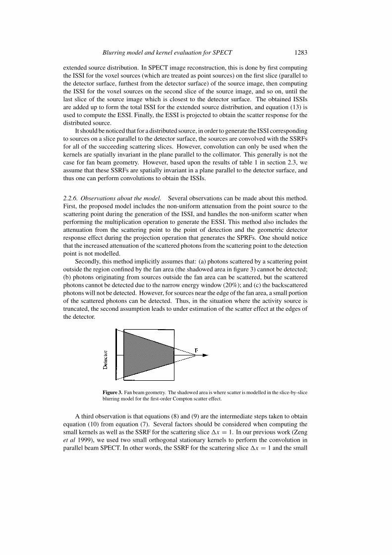
Secondly, this method implicitly assumes that: (a) photons scattered by a scattering pointoutside the region confined by the fan area (the shadowed area in figure 3) cannot be detected;(b) photons originating from sources outside the fan area can be scattered, but the scatteredphotons cannot be detected due to the narrow energy window (20%); and (c) the backscatteredphotons will not be detected. However, for sources near the edge of the fan area, a small portionof the scattered photons can be detected. Thus, in the situation where the activity source istruncated, the second assumption leads to under estimation of the scatter effect at the edges ofthe detector.

Figure 3. Fan beam geometry. The shadowed area is where scatter is modelled in the slice-by-sliceblurring model for the first-order Compton scatter effect.

A third observation is that equations (8) and (9) are the intermediate steps taken to obtainequation (10) from equation (7). Several factors should be considered when computing thesmall kernels as well as the SSRF for the scattering slice�x = 1. In our previous work (Zenget al 1999), we used two small orthogonal stationary kernels to perform the convolution inparallel beam SPECT. In other words, the SSRF for the scattering slice �x = 1 and the small

1284 C Bai et al

convolution kernels between the scattering slices were the same in equations (8) and (9), andthe kernels were independent of the position of the point source. In this work though, for aparticular scattering slice, the SSRFs and the small kernels are functions of the distance fromthe point source to the scattering slice. For converging beam geometry, the SSRFs and kernelsalso depend upon the focal length, the distance from the point source to the focal point, andthe distance to the converging beam central ray. Necessary information can be obtained fromthe transformed Klein–Nishina formula, which is obtained by substituting equation (5) intoequation (1).

In this work, we approximate the SSRFs with Gaussians, of which the full width at halfmaximum (FWHM) is determined by the energy window and the position of the point source.By knowing the SSRFs of two neighbouring scattering slices, the two small blurring kernels arecalculated assuming that the SSRF of the slice closer to the detector surface is the convolutionof the SSRF of the slice further from the detector surface with the two small kernels. Inthe implementation, these two small kernels are approximated by two small symmetric five-point 1D kernels which are calculated on the fly by knowing the FWHMs of the Gaussianapproximations of the SSRFs of the two slices.

Finally, the implementation of equations (6) and (12) to obtain the ISSI for each scatteringslice is the same as the implementation of the slice-by-slice blurring model that models both thedepth-dependent detector response and non-uniform attenuation effects (for example Bai et al1998a). In this paper, equation (12) is implemented in such a way that the scatter convolutionand the corresponding attenuation are performed at the same time, i.e. the value of a voxelon slice n + 1 is obtained by first multiplying the values of the voxels on slice n of the ISSIwith their corresponding elements in the convolution kernel, then weighting the results withthe attenuation from the voxels on slice n to the voxel on slice n + 1, and finally summingthem up. In this way, the modelling of non-uniform attenuation involves interpolations ofthe attenuation from the voxels in the previous slice to the voxel in the next slice, that is, theconvolved voxels of the previous slice that contribute to the voxel in the slice being calculatedare each weighted by an attenuation factor.

2.3. Computing the convolution kernels from the theoretical SSRFs

In this section we describe how Gaussian functions are used to approximate the theoreticalSSRF F(θ(yd,�x, xSS, ySS, f ), E) which is a function of the energy, geometry and position.(Note: F(θ(yd,�x, xSS, ySS, f ), E) reduces toGfan(yd,�x) for a given set of xSS, ySS,E andf .) From this Gaussian function the convolution kernels are calculated for the slice-by-sliceblurring model. The overall approach is to first calculate the theoretical SSRF, then multiplythe SSRF with the energy detection probability function P(ESC), where ESC is the energyof the scattered photon. This procedure results in a modulated SSRF with the assumption inStep 3 of section 2.1.2. The modulated SSRF has a value zero for an energy outside the givenenergy window, a maximum value 1.0 (maximum) for the photopeak energy and a minimumvalue (minimum) for the lower edge of the energy window. The full width at the value whichis half the sum of the maximum value and the minimum value of the modulated SSRF is usedas the FWHM of the Gaussian function which is used to approximate the SSRF.

For example, for a fan beam SPECT acquisition in which f = 104, E = 140 keV and a20% energy window (126–154 keV) is used, the SSRF is computed in the following way. First,from Compton scatter theory we compute the maximum scatter angle that corresponds to ascattered photon with energy of 126 keV, since this is the minimum energy that can be detectedfor a 20% energy window with the assumption in Step 3 of section 2.1.2. For 126 keV thisangle is 53.53◦. For this angle the energy- and scatter-dependent factor in the Klein–Nishina

Blurring model and kernel evaluation for SPECT 1285

formula in equation (1) isF(53.53◦, 140) = 0.55. A Gaussian function is used to approximatethe portion of SSRFGfan(yd,�x) (now only a function of yd ) that will fall within the windowof 0.55 (minimum) to 1.0 (maximum) for a given set of �x, xSS, ySS, E and f . In order tosimplify the calculation we simply calculate the width of the SSRF at the value of 0.778, whichis half of the sum of the minimum value of 0.55 and the maximum value of 1.0 and use thiswidth as the FWHM of the Gaussian approximation of the modulated SSRF. Note that this isdone for point sources that are not too close to the focal line.

Appendix B discusses the approximation of SSRFs using Gaussian functions when thecorrect energy detection probability function P(ESC) is used instead of using the windowfunction assumption in Step 3 of section 2.1.2. The discussion shows results that are onlyslightly different from the results in this section.

The FWHM of the Gaussian approximation is a function of point source position (xSS, ySS),the distance of the scattering slice to the point source �x, and the focal length. Table 1 givesexamples of the FWHMs of the Gaussians, for varying�x, varying xSS and varying ySS. Fromtable 1 it is apparent that, for a given point source position, the FWHM is approximatelyproportional to �x, that is

FWHM(�x, xSS, ySS) = FWHM(1, xSS, ySS)�x. (15)

Table 1. Computed FWHMs for Gaussian approximation of SSRFs. f = 104 bins, E = 140 keV,20% energy window; unit: bin (sampling unit on the detector surface). Note: the centre ray of thefan beam geometry is when the second coordinate is zero.

(xSS, ySS)

�x (10, 0) (26, 0) (42, 0) (58, 0) (74, 0) (42, 0) (42, 5) (42, 10) (42, 15) (42, 20)

1 1.44 1.74 2.19 2.95 4.55 2.19 2.21 2.27 2.37 2.542 2.89 3.49 4.40 5.99 9.26 4.40 4.45 4.58 4.81 5.143 4.35 5.27 6.66 9.05 14.15 6.66 6.72 6.94 7.30 7.834 5.84 7.07 8.95 12.21 19.25 8.95 9.04 9.34 9.85 10.625 7.33 8.89 11.28 15.45 24.64 11.28 11.41 11.80 12.48 13.52

For �x = 1, the FWHM depends on both xSS and ySS. Therefore, one can compute for agiven focal length, photon energy and detection energy window, a look-up table for the FWHMsfor�x = 1 at different xSS and ySS. However, one can also compute the FWHMs and fit themto a function of (�x, xSS, ySS, f, E), thereby avoiding the look-up table and computing theFWHMs on the fly. Another possibility is to derive the function from the transformed Klein–Nishina formula by using an appropriate approximation. In the parallel direction, the FWHMfor �x = 1 is independent of the point source position, and its value is 1.32 bins.

The small blurring kernels (described in section 2.2.2) are calculated by using the knownexpression for the FWHM as a function of distance from the detector. These kernels can becomputed by using a least squares method (Bai et al 1997), or by using Gaussian samplingwith appropriate normalization, considering the fact that convolution of two Gaussian functionsresults in another Gaussian function, and the resultant Gaussian function has an integral thatis the product of the integrals of the two original Gaussian functions. One should also notethat the Gaussian functions used to compute the small convolution kernels are normalized (Baiet al 1997, Zeng et al 1998). However, as shown in equation (15), the Gaussian functions usedto approximate the SSRFs have a maximum value of 1, and FWHMs that are proportional to�x. Therefore, the normalization of the obtained Gaussian functions should be considered.This is shown in Appendix A.

1286 C Bai et al

It is shown in table 1 that the FWHMs of the Gaussian approximations increase as thesource is moved off the central ray of the fan beam geometry. And it is also observed thatthe SSRFs become more asymmetrical as the source is moved further off the central ray.However, the increase in the width of the Gaussian approximation is comparatively small, andthe asymmetry of the SSRFs occurs when the scattering angle is comparatively large. Thus, onecan assume that the Gaussian approximations for the voxel sources on a source slice (parallelto the detector surface) of the source image are the same. Therefore, in the implementation ofequations (6) and (10), one can perform the convolution using the same kernels for the voxelsources in the same source slice.

3. Methods

3.1. Evaluation of the model using Monte Carlo simulations

3.1.1. Scatter point response functions (SPRFs) for parallel beam geometry. Monte Carlosimulations were performed using PHG Release 2.5b (Vannoy 1994) to generate first-orderCompton scatter for parallel beam geometry, using the non-uniform attenuator of the MCATphantom (Terry et al 1990) as the scattering object. The ESSIs generated from the proposedslice-by-slice blurring model were projected to give the scatter point responses, using aprojector that also modelled attenuation but not geometric detector response as described insection 2.2.5. Also, the scatter projection was generated using the slice-by-slice blurring modelproposed in our previous work (Zeng et al 1999). First-order Compton scatter point responsesobtained from MC simulations and the slice-by-slice blurring models were compared.

3.1.2. Scatter point response functions (SPRFs) for fan beam geometry. The proposed slice-by-slice blurring model was used to generate a set of first-order Compton scatter projections forfan beam geometry. A Monte Carlo (MC) simulation was performed to generate the Comptonscattered projections from first-order to sixth-order. The summation of the Compton scatterprojections from first-order to sixth-order was used to approximate the full Monte Carlo (fMC)result. The scatter projections generated using the proposed model were compared with the MCfirst-order Compton scatter projections and also compared with the fMC scatter projections.

3.1.3. Scatter response of a distributed source for fan beam geometry. In order to evaluatethe application of the model to a distributed source, the MCAT phantom was used with activitypresent only in the cardiac walls. The proposed slice-by-slice blurring model was used togenerate a set of first-order Compton scatter projections for fan beam geometry. A MonteCarlo (MC) simulation was performed to generate the Compton scattered projections fromfirst-order to sixth-order. The summation of the Compton scatter projections from first-order tosixth-order was used to approximate the full Monte Carlo (fMC) result. The scatter projectionsgenerated using the proposed model were compared with the MC first-order Compton scatterprojections and also compared with the fMC scatter projections.

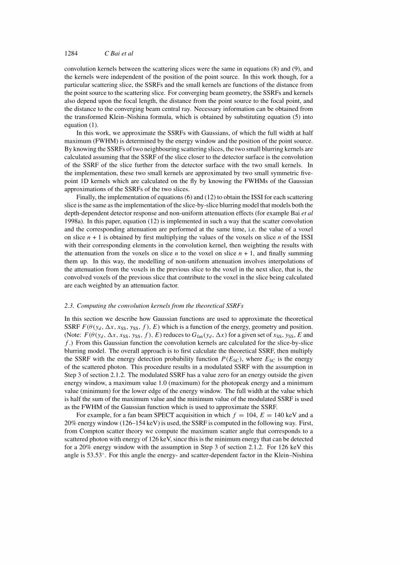
Figure 4 shows slices of the attenuation map of the MCAT phantom, the detector positionsand the sources. First-order Compton scattered photons were detected from four angles (0◦,90◦, 180◦ and 270◦), which corresponded to the detector positions 1, 2, 3 and 4 respectively.The geometric detector response was not simulated because our focus was on evaluating howwell the incremental blurring technique performs in modelling only first-order Compton scatter.The bin size was 0.625 cm, the attenuation map was a 64× 64× 64 matrix and a circular orbitwith a radius of 22.0 cm was used. The energy window was ±10%, centred at 140 keV. Forfan beam geometry, the point source was positioned so that, at detector positions 1 and 3, the

Blurring model and kernel evaluation for SPECT 1287

Figure 4. Slices of the attenuation map of the MCAT phantom and sources. Top left: point sourcefor parallel beam geometry. Top right: point source for fan beam geometry. The point source isin a different transaxial slice from that for parallel beam geometry. Bottom: distributed source forfan beam geometry. Scatter projection data are acquired at four detection angles denoted by 1, 2,3 and 4 for all cases.

Figure 5. Phantom used for physical point source scan using fan-beam SPECT: (a) a transaxialcross section of the phantom; (b) an axial cross section of the phantom.

point source was almost on the central ray, and at detector positions 0 and 2, the point sourcewas approximately 10 bins from the central ray. The focal length was 65.0 cm.

3.2. Evaluation of the model using physical fan beam point source data

A point source scan was performed using a Picker PRISM 3000XP three-head SPECT system(Picker International, Cleveland, OH) with fan beam collimation. The point source, withan activity of 4.77 MBq (130 µCi) of 99mTc, was put at approximately the centre of a non-uniform phantom a shown in figure 5. The measured point responses were compared withthe responses generated using slice-by-slice blurring model, which modelled non-uniformattenuation, geometric point response and non-uniform first-order Compton scatter.

The activity was contained in a capillary glass tube which was approximately 1.5 cm longand sealed at both ends. The activity was confined within a 1 mm length of the tube. The remain-der of the tube was empty. The design of the phantom was based on two considerations: (a) thepresence of non-uniform scattering media and (b) the ease of inserting and removing the point

1288 C Bai et al

(a)

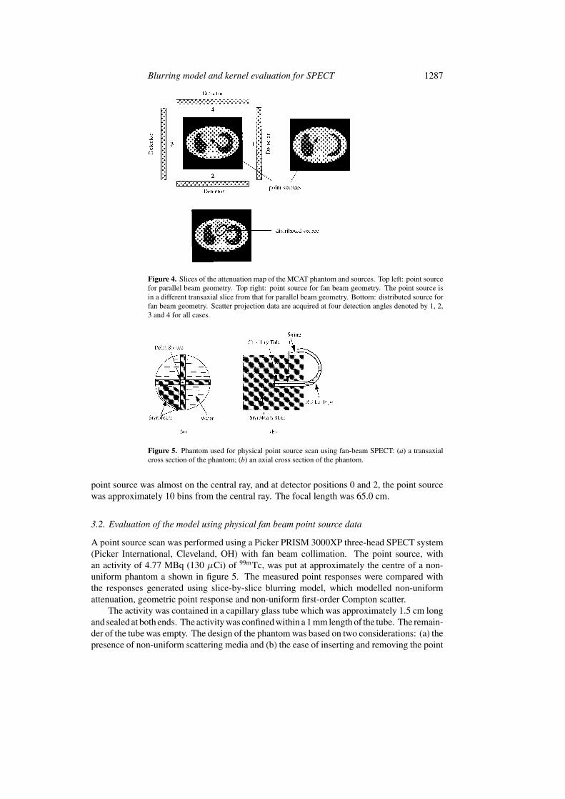
Figure 6. Scatter point responses in parallel beam SPECT. (a) Profiles of scatter point responses.Vertical axis: absolute scale, arbitrary units. Horizontal axis: bin number. Broad solid line:the proposed model, varying kernels. Thin solid line: MC. Thin dashed line: stationary kernels(Zeng et al 1999). The number at the shoulder of each profile corresponds to the detector positionshown in figure 4. (b) Semi-log profiles of scatter point responses. Vertical axis: logarithm ofthe reconstructed intensity. Horizontal axis: bin number. Broad solid line: the proposed model,varying kernels. Thin solid line: MC. Thin dashed line: stationary kernels (Zeng et al 1999). Thenumber at the shoulder of each profile corresponds to the detector position shown in figure 4.

source. In order to prepare the non-uniform phantom, two slices of Styrofoam were combinedto form a Styrofoam cross. The Styrofoam cross was put into a hollow cylindrical container(a Deluxe ECT phantom (Data Spectrum, Hillsborough, NC) with the inserts taken out), whichdivided the container into four sectors. Then a loaf-like Styrofoam piece of irregular shapewas put into one of the sectors. Half of the intersecting line of the two Styrofoam slices was cutaway, so that the capillary tube could be inserted into the Styrofoam cross at different positions.After the capillary tube was placed in the Styrofoam cross, the container was filled with water.

A flexible rubber pipe was plugged into the central hole of the lid of the cylindricalcontainer. The end of the capillary tube that was outside the Styrofoam was tied with string.The string was guided out of the container through the flexible pipe. In this way, the capillarytube could be pulled out of the container by pulling the string, without opening the container.Figure 5 illustrates a transaxial cross section and an axial cross section of the phantom.

Blurring model and kernel evaluation for SPECT 1289

(b)

Figure 6. (Continued)

Table 2. Scatter to primary ratios of the scatter point responses for parallel beam SPECT(MC, Monte Carlo results; BL, proposed blurring model results). The numbers in the first rowcorrespond to the detector positions shown in figure 4. The last row is the percentage difference:(BL −MC)/MC× 100%.

1 2 3 4

MC 0.568 0.565 0.452 0.330BL 0.555 0.580 0.439 0.336% −2.3 + 2.6 −3.0 + 1.8

The emission scan was performed from four angles (uniformly distributed over 360◦),using one of the three heads of the SPECT system. The scanning time was 30 s for each stop.The projection bin size was 0.712 cm. The energy window was ±7.5% centred at 140 keV,and a circular orbit of a radius of 20.9 cm was used.

After the emission scan, the capillary tube was pulled out of the phantom. A transmissionscan was performed using a transmission line source of activity 633 MBq (17.25 mCi) of99mTc that was put at the focal line of the corresponding collimator. The transmission datawere acquired from 120 angles with an angular separation of 3◦ between two consecutiveangles. The total transmission scan time was 20 min.

1290 C Bai et al

(a)

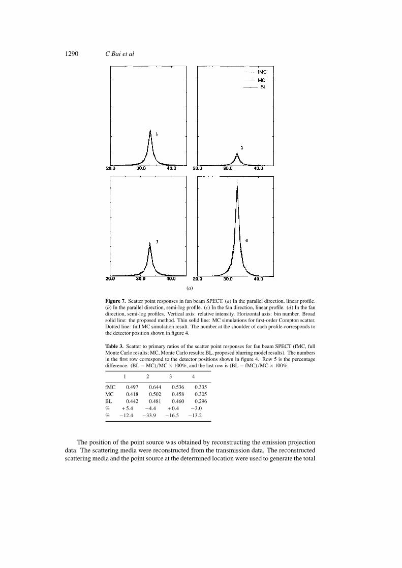
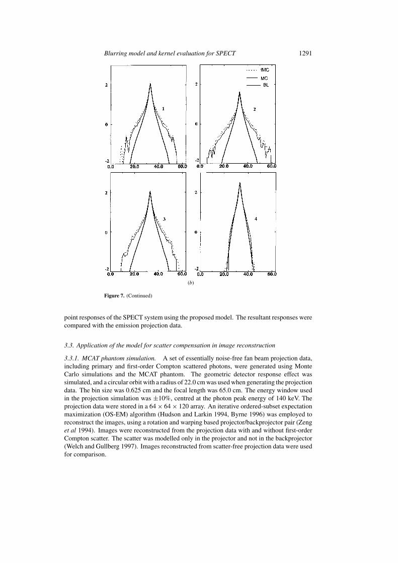
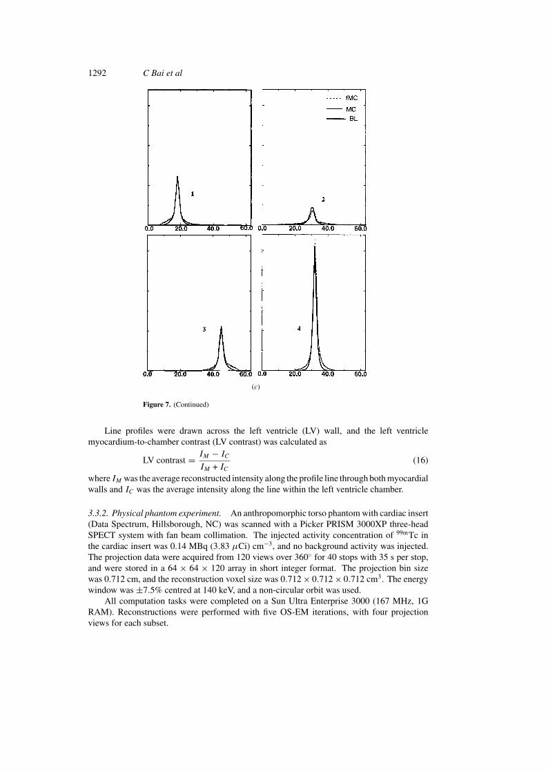
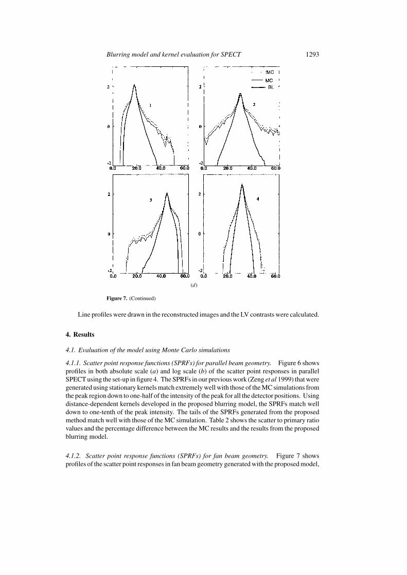
Figure 7. Scatter point responses in fan beam SPECT. (a) In the parallel direction, linear profile.(b) In the parallel direction, semi-log profile. (c) In the fan direction, linear profile. (d) In the fandirection, semi-log profiles. Vertical axis: relative intensity. Horizontal axis: bin number. Broadsolid line: the proposed method. Thin solid line: MC simulations for first-order Compton scatter.Dotted line: full MC simulation result. The number at the shoulder of each profile corresponds tothe detector position shown in figure 4.

Table 3. Scatter to primary ratios of the scatter point responses for fan beam SPECT (fMC, fullMonte Carlo results; MC, Monte Carlo results; BL, proposed blurring model results). The numbersin the first row correspond to the detector positions shown in figure 4. Row 5 is the percentagedifference: (BL −MC)/MC× 100%, and the last row is (BL − fMC)/MC× 100%.

1 2 3 4

fMC 0.497 0.644 0.536 0.335MC 0.418 0.502 0.458 0.305BL 0.442 0.481 0.460 0.296% + 5.4 −4.4 + 0.4 −3.0% −12.4 −33.9 −16.5 −13.2

The position of the point source was obtained by reconstructing the emission projectiondata. The scattering media were reconstructed from the transmission data. The reconstructedscattering media and the point source at the determined location were used to generate the total

Blurring model and kernel evaluation for SPECT 1291

(b)

Figure 7. (Continued)

point responses of the SPECT system using the proposed model. The resultant responses werecompared with the emission projection data.

3.3. Application of the model for scatter compensation in image reconstruction

3.3.1. MCAT phantom simulation. A set of essentially noise-free fan beam projection data,including primary and first-order Compton scattered photons, were generated using MonteCarlo simulations and the MCAT phantom. The geometric detector response effect wassimulated, and a circular orbit with a radius of 22.0 cm was used when generating the projectiondata. The bin size was 0.625 cm and the focal length was 65.0 cm. The energy window usedin the projection simulation was ±10%, centred at the photon peak energy of 140 keV. Theprojection data were stored in a 64× 64× 120 array. An iterative ordered-subset expectationmaximization (OS-EM) algorithm (Hudson and Larkin 1994, Byrne 1996) was employed toreconstruct the images, using a rotation and warping based projector/backprojector pair (Zenget al 1994). Images were reconstructed from the projection data with and without first-orderCompton scatter. The scatter was modelled only in the projector and not in the backprojector(Welch and Gullberg 1997). Images reconstructed from scatter-free projection data were usedfor comparison.

1292 C Bai et al

(c)

Figure 7. (Continued)

Line profiles were drawn across the left ventricle (LV) wall, and the left ventriclemyocardium-to-chamber contrast (LV contrast) was calculated as

LV contrast = IM − ICIM + IC

(16)

where IM was the average reconstructed intensity along the profile line through both myocardialwalls and IC was the average intensity along the line within the left ventricle chamber.

3.3.2. Physical phantom experiment. An anthropomorphic torso phantom with cardiac insert(Data Spectrum, Hillsborough, NC) was scanned with a Picker PRISM 3000XP three-headSPECT system with fan beam collimation. The injected activity concentration of 99mTc inthe cardiac insert was 0.14 MBq (3.83 µCi) cm−3, and no background activity was injected.The projection data were acquired from 120 views over 360◦ for 40 stops with 35 s per stop,and were stored in a 64 × 64 × 120 array in short integer format. The projection bin sizewas 0.712 cm, and the reconstruction voxel size was 0.712× 0.712× 0.712 cm3. The energywindow was ±7.5% centred at 140 keV, and a non-circular orbit was used.

All computation tasks were completed on a Sun Ultra Enterprise 3000 (167 MHz, 1GRAM). Reconstructions were performed with five OS-EM iterations, with four projectionviews for each subset.

Blurring model and kernel evaluation for SPECT 1293

(d)

Figure 7. (Continued)

Line profiles were drawn in the reconstructed images and the LV contrasts were calculated.

4. Results

4.1. Evaluation of the model using Monte Carlo simulations

4.1.1. Scatter point response functions (SPRFs) for parallel beam geometry. Figure 6 showsprofiles in both absolute scale (a) and log scale (b) of the scatter point responses in parallelSPECT using the set-up in figure 4. The SPRFs in our previous work (Zeng et al 1999) that weregenerated using stationary kernels match extremely well with those of the MC simulations fromthe peak region down to one-half of the intensity of the peak for all the detector positions. Usingdistance-dependent kernels developed in the proposed blurring model, the SPRFs match welldown to one-tenth of the peak intensity. The tails of the SPRFs generated from the proposedmethod match well with those of the MC simulation. Table 2 shows the scatter to primary ratiovalues and the percentage difference between the MC results and the results from the proposedblurring model.

4.1.2. Scatter point response functions (SPRFs) for fan beam geometry. Figure 7 showsprofiles of the scatter point responses in fan beam geometry generated with the proposed model,

1294 C Bai et al

(a)

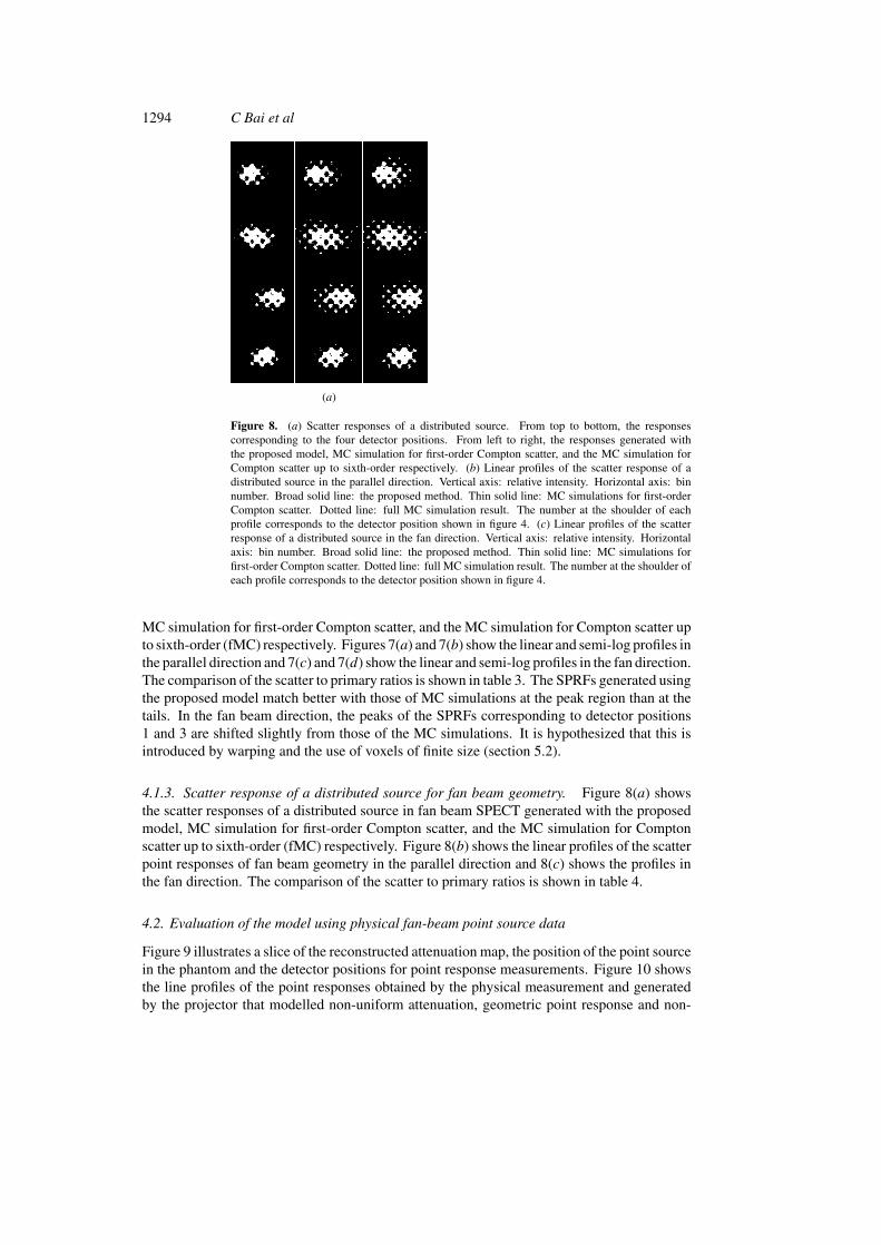
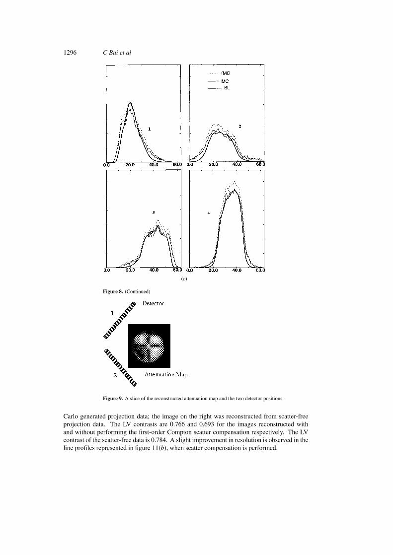
Figure 8. (a) Scatter responses of a distributed source. From top to bottom, the responsescorresponding to the four detector positions. From left to right, the responses generated withthe proposed model, MC simulation for first-order Compton scatter, and the MC simulation forCompton scatter up to sixth-order respectively. (b) Linear profiles of the scatter response of adistributed source in the parallel direction. Vertical axis: relative intensity. Horizontal axis: binnumber. Broad solid line: the proposed method. Thin solid line: MC simulations for first-orderCompton scatter. Dotted line: full MC simulation result. The number at the shoulder of eachprofile corresponds to the detector position shown in figure 4. (c) Linear profiles of the scatterresponse of a distributed source in the fan direction. Vertical axis: relative intensity. Horizontalaxis: bin number. Broad solid line: the proposed method. Thin solid line: MC simulations forfirst-order Compton scatter. Dotted line: full MC simulation result. The number at the shoulder ofeach profile corresponds to the detector position shown in figure 4.

MC simulation for first-order Compton scatter, and the MC simulation for Compton scatter upto sixth-order (fMC) respectively. Figures 7(a) and 7(b) show the linear and semi-log profiles inthe parallel direction and 7(c) and 7(d) show the linear and semi-log profiles in the fan direction.The comparison of the scatter to primary ratios is shown in table 3. The SPRFs generated usingthe proposed model match better with those of MC simulations at the peak region than at thetails. In the fan beam direction, the peaks of the SPRFs corresponding to detector positions1 and 3 are shifted slightly from those of the MC simulations. It is hypothesized that this isintroduced by warping and the use of voxels of finite size (section 5.2).

4.1.3. Scatter response of a distributed source for fan beam geometry. Figure 8(a) showsthe scatter responses of a distributed source in fan beam SPECT generated with the proposedmodel, MC simulation for first-order Compton scatter, and the MC simulation for Comptonscatter up to sixth-order (fMC) respectively. Figure 8(b) shows the linear profiles of the scatterpoint responses of fan beam geometry in the parallel direction and 8(c) shows the profiles inthe fan direction. The comparison of the scatter to primary ratios is shown in table 4.

4.2. Evaluation of the model using physical fan-beam point source data

Figure 9 illustrates a slice of the reconstructed attenuation map, the position of the point sourcein the phantom and the detector positions for point response measurements. Figure 10 showsthe line profiles of the point responses obtained by the physical measurement and generatedby the projector that modelled non-uniform attenuation, geometric point response and non-

Blurring model and kernel evaluation for SPECT 1295

(b)

Figure 8. (Continued)

Table 4. Scatter to primary ratios of the scatter responses of a distributed source for fan beamSPECT (fMC, full Monte Carlo results; MC, Monte Carlo results; BL, proposed blurring modelresults). The numbers in the first row correspond to the detector positions shown in figure 4. Row 5is the percentage difference: (BL−MC)/MC×100%, and the last row is (BL−fMC)/MC×100%.

1 2 3 4

fMC 0.559 0.775 0.617 0.362MC 0.471 0.631 0.514 0.323BL 0.502 0.610 0.524 0.310% + 6.6 −3.3 + 2.0 −4.0% −11.4 −27.0 −17.7 −16.8

uniform first-order Compton scatter effects. Line profiles were drawn in both parallel and fandirections.

4.3. Application of the model for scatter compensation in image reconstruction

4.3.1. MCAT phantom simulation. The same transaxial slices of the images are displayedin figure 11(a) as follows: left and centre images show, respectively, the reconstructionswithout and with performing the first-order Compton scatter compensation from the Monte

1296 C Bai et al

(c)

Figure 8. (Continued)

Figure 9. A slice of the reconstructed attenuation map and the two detector positions.

Carlo generated projection data; the image on the right was reconstructed from scatter-freeprojection data. The LV contrasts are 0.766 and 0.693 for the images reconstructed withand without performing the first-order Compton scatter compensation respectively. The LVcontrast of the scatter-free data is 0.784. A slight improvement in resolution is observed in theline profiles represented in figure 11(b), when scatter compensation is performed.

Blurring model and kernel evaluation for SPECT 1297

(a)

(b)

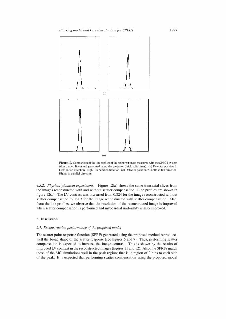
Figure 10. Comparison of the line profiles of the point responses measured with the SPECT system(thin dashed lines) and generated using the projector (thick solid lines). (a) Detector position 1.Left: in fan direction. Right: in parallel direction. (b) Detector position 2. Left: in fan direction.Right: in parallel direction.

4.3.2. Physical phantom experiment. Figure 12(a) shows the same transaxial slices fromthe images reconstructed with and without scatter compensation. Line profiles are shown infigure 12(b). The LV contrast was increased from 0.824 for the image reconstructed withoutscatter compensation to 0.903 for the image reconstructed with scatter compensation. Also,from the line profiles, we observe that the resolution of the reconstructed image is improvedwhen scatter compensation is performed and myocardial uniformity is also improved.

5. Discussion

5.1. Reconstruction performance of the proposed model

The scatter point response function (SPRF) generated using the proposed method reproduceswell the broad shape of the scatter response (see figures 6 and 7). Thus, performing scattercompensation is expected to increase the image contrast. This is shown by the results ofimproved LV contrast in the reconstructed images (figures 11 and 12). Also, the SPRFs matchthose of the MC simulations well in the peak region; that is, a region of 2 bins to each sideof the peak. It is expected that performing scatter compensation using the proposed model

1298 C Bai et al

(a)

(b)

Figure 11. MCAT phantom study. (a) Same slices of the reconstructed images. Left:reconstructed without scatter compensation. Centre: reconstructed with scatter compensation.Right: reconstructed from scatter-free data. (b) Line profiles along the line shown in (a). Thindashed line: without scatter compensation. Broad solid line: with scatter compensation. Thinsolid line: reconstructed from scatter-free data (gold standard).

gives some improvement in resolution even if geometric response is modelled. In the MCATphantom study, images reconstructed with scatter compensation exhibit a slight improvementin the resolution of the left ventricle walls. Line profiles in figure 12 of the Jaszczak phantomexperiment demonstrate an obvious resolution improvement of the left ventricle walls whenimages were reconstructed with scatter compensation in addition to attenuating and detectorresponse compensation.

5.2. SPRFs for fan beam geometry

The spatial scatter response functions (SSRFs) for fan beam geometry are asymmetric whenthe point source is not located on the central ray of the converging beam. One may expectlarger errors when the point source is farther away from the central ray when using Gaussiansto approximate the SSRFs. However, because only the photons that scatter in a small angularrange can be detected due to the narrow energy window, the SSRFs are symmetric in the spatialregion that corresponds to this small angular range. Therefore, Gaussian approximation is agood approximation (see also appendix B).

In converging beam SPECT, a point source is set on the centre of a voxel to generate theSPRFs. However, when a rotation and warping based projector is used, the position of thepoint source after rotation and warping can be anywhere in a new voxel. The activity image is

Blurring model and kernel evaluation for SPECT 1299

(a)

(b)

Figure 12. Physical phantom experiments. The images were zoomed for display. (a) Sameslices from the images reconstructed with (right) and without (left) scatter compensation using theproposed method. (b) Line profiles along the line shown in (a). Thin dashed line: without scattercompensation. Broad solid line: with scatter compensation.

voxelized and the projection is performed based on the newly transformed activity distribution.Therefore a small shift in the SPRFs may result. This is shown by the shift of the peaks infan beam SPRFs for detector positions 1 and 3 compared with the MC results displayed infigure 7. The shift decreases when the voxel size decreases.

5.3. Attenuation effect at different photon energies

In equation (14) it is assumed that Compton scatter dominates the attenuation coefficient inSPECT when the photon energy is high. In table 5 we list the ratio of the attenuation effect dueto photoelectric absorption to the attenuation effect due to Compton scatter for water, brain andfat at energies of 140 keV, 90 keV and 10 keV calculated using the equations and the valuesgiven in the work of Alvarez and Macovski (1976). For a variety of other human tissues, therelative attenuation effect due to the photoelectric absorption to the Compton scatter effect isnearly the same as for brain and water. One can check the results of water with those given bySorenson and Phelps (1987).

For bone, because of its higher effective atomic number (effective Z number), thephotoelectric absorption can be much greater than that of water or other human tissues.However, bone accounts for only a small portion of the torso, so the error introduced by the high

1300 C Bai et al

Table 5. Ratios of the attenuation effect due to photoelectric absorption to that due to Comptonscatter.

E (keV) Water Brain Fat Bone

10 21.85 22.03 12.52 140.5790 0.038 0.038 0.022 0.24

140 0.011 0.011 0.007 0.07

photoelectric effect of bones can be neglected. For lungs, their composition changes in a largerange, and Compton scatter dominates the attenuation effect due to the low atomic number.

5.4. Increased attenuation for the scattered photons

The energies of the scattered photons are generally lower than those of the incident photons,therefore the attenuation along the same photon path in scattering media is more for thescattered photons than for the primary ones. This effect has been studied by Frey and Tsui(1996). However, in this work, this effect was not modelled.

5.5. Computation time

For parallel beam SPECT, the scatter point response functions (SPRFs) simulated using thedistance-dependent kernels in the proposed blurring model and the stationary kernels used inour previous work (Zeng et al 1999) agree extremely well with the results from MC simulationsthat include only first-order Compton scatter from the peak intensity down to one-half of thepeak intensity in the peak regions, and also agree well in the tail regions (figure 6). However,the time required to generate an SPRF using the varying kernels in the proposed model isapproximately 32 times as long as the time required when using stationary kernels (Zeng et al1999). Therefore, while it takes approximately 1 s to generate a 64 × 64 SPRF using thestationary kernels, it takes 32 s when using the varying kernels. It is observed that when�x isgreater than 5, the small blurring kernels are essentially stationary. The spatially varying kernelsare significantly different from the stationary kernels only when �x is less than or equal to 3.For a given point source and for the first few scattering slices (�x = 1, 2, 3, 4, 5), the centralelement of the blurring kernel is different from the side elements, and the difference decreasesas�x increases. When�x is greater than 5, the central element is essentially the same as theside elements. That being the case, one can apply stationary kernels when �x is greater than5. Based on this observation, the slice-by-slice blurring can be accelerated by using spatiallyvarying kernels up to �x = 5, and stationary kernels after. In this way the computation timefor generating the SPRF can be reduced by a factor of 5. This is also applicable to fan beamgeometry. The total reconstruction time required when only attenuation compensation and 3Dgeometric detector response compensation are performed is 5.2 s per slice per iteration. When3D scatter compensation is also performed, the reconstruction time per slice per iteration is6.9 s when using the stationary model (parallel beam SPECT), 60 s when using the spatiallyvarying kernels and approximately 16 s when stationary kernels are used after �x = 5.

The acceleration procedure is only needed for distributed sources. The implementationof this procedure is as follows: for each source slice which is parallel to the detector surface,the ISSIs for the scattering slices �x = 1, 2, 3, 4 are computed. We call these the first partof the ISSI for that particular source slice. The first parts of the ISSIs for all the source slicesare generated and appropriately added up to form the first part of the ISSI for the distributedsource. The ISSIs for the scattering slice �x = 5 for all the source slices are stored in a newarray to which an incremental blurring using stationary kernels can be applied (Zeng et al

Blurring model and kernel evaluation for SPECT 1301

1999) to generate the second part of the ISSI for the distributed source. Combining the firstpart and the second part of the ISSI gives the total ISSI for the distributed source, which canthen be used to generate the ESSI. Therefore the time required to generate the ISSI is about sixtimes longer than when stationary kernels are used (Zeng et al 1999). The acceleration factoris about five when the transaxial slice of the source image has a dimension of 64× 64, and tenwhen the transaxial slice of the source image has a dimension of 128× 128.

5.6. Application of the model for different agents

The proposed slice-by-slice blurring model has been developed for the modelling of first-orderCompton scatter in SPECT with the detection energy window centred at the photopeak energy.For a non-photopeak detection energy window, the energy-detection-probability-modulatedSSRFs (see appendix B) do not have a simple shape (a modulated SSRF usually has twopeaks), thus the proposed model cannot be simply applied to model the scatter for the non-photopeak energy window. For SPECT imaging using emission agents such as 99mTc, thedetection energy window is centred at the photopeak energy and the model can be applieddirectly. For some agents, 201Tl for example which has multiple emission energy peaks, thephotons down-scattered from higher energy peaks can be detected in the detection energywindow of the lower energy peaks. These parts of the scattered photons cannot be estimatedby a direct application of the model. For 201Tl backscatter is a significant contributor to thescatter response, and our scatter model in the current form cannot be applied. In our futurework, the model will be modified so that it can be used to model the down-scattered eventsand also backscattered events in SPECT.

6. Conclusions

In this work we have developed a method to model first-order Compton scatter in parallel andconverging beam SPECT. The scattering angle in the Klein–Nishina formula is expressed interms of the positions of the point source, scattering point, detection point and the geometricfocus, so that the spatial scatter response function (SSRF) and the intermediate scatter sourceimage (ISSI) of a scattering slice to the point source can be computed. By convolving this ISSIwith two orthogonal small 1D kernels, the ISSI of the next scattering slice, which is closerto the detector surface, can be approximated. An effective scatter source image (ESSI) canthan be obtained from the ISSI. The scatter point response function (SPRF) is generated byprojecting the ESSI to the detector with a projector modelling both attenuation and geometricdetector response effects. The proposed slice-by-slice blurring model has been evaluatedusing Monte Carlo simulation studies and physical phantom experiments. The scatter pointresponse functions (SPRFs) generated using the proposed model match well with those ofthe MC simulations that include only first-order Compton scatter for both parallel and fanbeam geometries. For fan beam geometry, images reconstructed from the projection datagenerated by MC simulations using the MCAT phantom with the first-order Compton scattereffect present a higher LV contrast (0.766) when scatter compensation is performed than whenit is not performed (0.693). Slight improvement in the image resolution is also observed.Physical phantom experiments using a large Jaszczak torso phantom show that the LV contrastis increased from 0.824, when no scatter compensation is performed, to 0.903 when the scattercompensation using the proposed model is performed. Image resolution and myocardialuniformity are also improved by performing scatter compensation. The proposed incrementalblurring model provides an efficient method for first-order Compton scatter compensation inboth parallel and converging beam SPECT.

1302 C Bai et al

Appendix A. Discrete implementation of the model

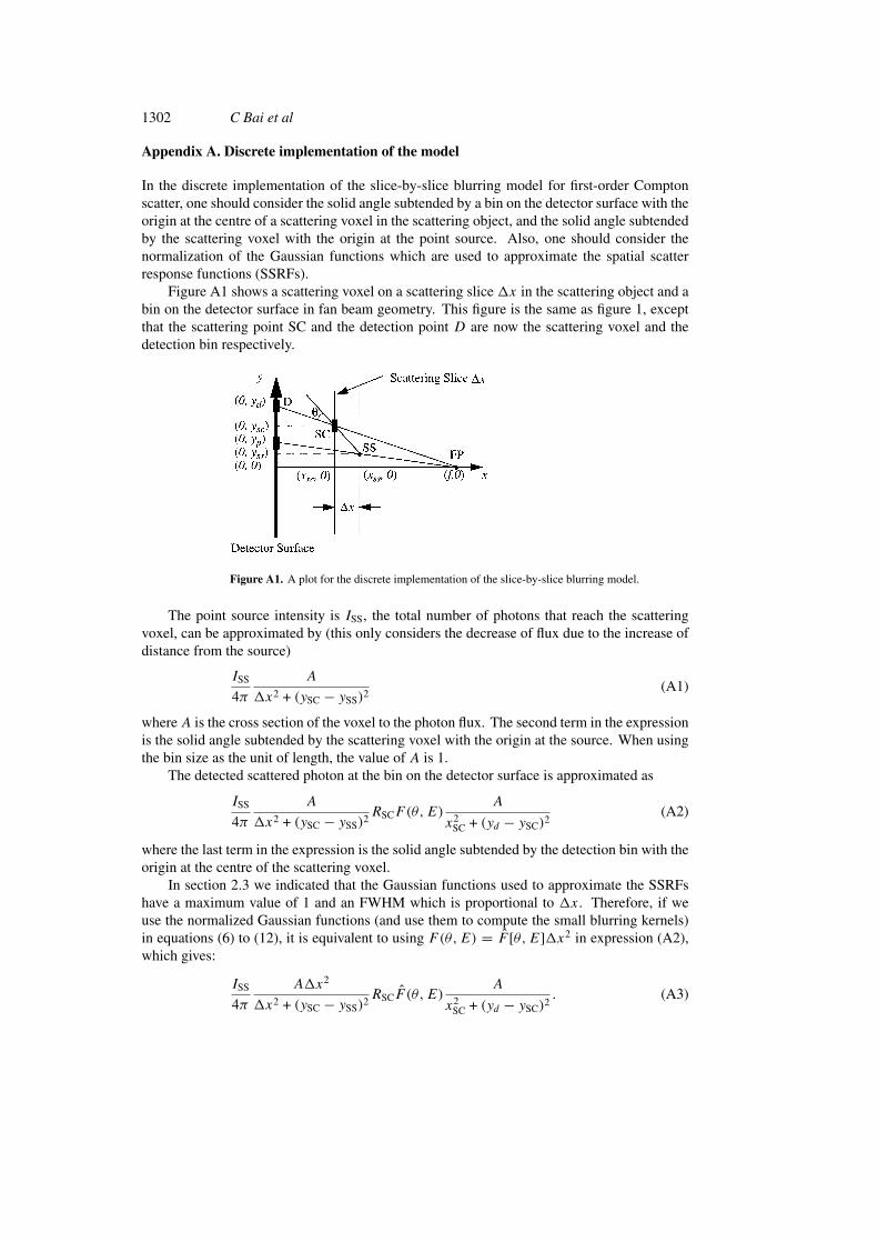
In the discrete implementation of the slice-by-slice blurring model for first-order Comptonscatter, one should consider the solid angle subtended by a bin on the detector surface with theorigin at the centre of a scattering voxel in the scattering object, and the solid angle subtendedby the scattering voxel with the origin at the point source. Also, one should consider thenormalization of the Gaussian functions which are used to approximate the spatial scatterresponse functions (SSRFs).

Figure A1 shows a scattering voxel on a scattering slice �x in the scattering object and abin on the detector surface in fan beam geometry. This figure is the same as figure 1, exceptthat the scattering point SC and the detection point D are now the scattering voxel and thedetection bin respectively.

Figure A1. A plot for the discrete implementation of the slice-by-slice blurring model.

The point source intensity is ISS, the total number of photons that reach the scatteringvoxel, can be approximated by (this only considers the decrease of flux due to the increase ofdistance from the source)

ISS

4π

A

�x2 + (ySC − ySS)2(A1)

whereA is the cross section of the voxel to the photon flux. The second term in the expressionis the solid angle subtended by the scattering voxel with the origin at the source. When usingthe bin size as the unit of length, the value of A is 1.

The detected scattered photon at the bin on the detector surface is approximated as

ISS

4π

A

�x2 + (ySC − ySS)2RSCF(θ,E)

A

x2SC + (yd − ySC)2

(A2)

where the last term in the expression is the solid angle subtended by the detection bin with theorigin at the centre of the scattering voxel.

In section 2.3 we indicated that the Gaussian functions used to approximate the SSRFshave a maximum value of 1 and an FWHM which is proportional to �x. Therefore, if weuse the normalized Gaussian functions (and use them to compute the small blurring kernels)in equations (6) to (12), it is equivalent to using F(θ,E) = F̂ [θ, E]�x2 in expression (A2),which gives:

ISS

4π

A�x2

�x2 + (ySC − ySS)2RSCF̂ (θ, E)

A

x2SC + (yd − ySC)2

. (A3)

Blurring model and kernel evaluation for SPECT 1303

For the detection of primary photons one should also consider the solid angle subtendedby the detection bin (0, yp) with the origin at the source. The flux to the detection bin (withoutattenuation) is

ISS

4π

A

x2SS + (yp − ySS)2

. (A4)

Dividing expression (A3) by (A4) and taking into account that A = 1, one can obtain(�x2

�x2 + (ySC − ySS)2

x2SS + (yp − ySS)

2

x2SC + (yd − ySC)2

)RSCF̂ (θ, E). (A5)

This illustrates how to modify equation (13) in the discrete implementation of the slice-by-slice blurring model, in order to obtain the correct quantitation (scatter-to-primary ratio). Themodification is done by multiplying each scattering voxel by its corresponding factor given bythe term in the large brackets in expression (A5):

�x2

�x2 + (ySC − ySS)2

x2SS + (yp − ySS)

2

x2SC + (yd − xSC)2

. (A6)

In our implementation, we approximate the first term in expression (A6) by 1, andapproximate the second term in (A6) by x2

SS/x2SC, therefore expression (A6) is simplified

to

x2SS

x2SC

. (A7)

In each projection view, the computation of ISSI is the same as described from equation (6)to equation (12). Then computation of ESSI using equation (13) is performed by thevoxel-wise multiplication by the composition-dependent scatter factor and the factor givenby expression (A7). For a distributed source, in order to decrease the computation, themultiplication by the factor in (A7) is performed first for each source position by performinga multiplication by x2

SS for all the scattering slices, then dividing by x2SC for each slice after

the sum has been performed over all sources. In this way the division step does not have to beperformed in the calculation at each source position.

Another way to simplify expression (A6) is to integrate the first term into the SSRFs togive spatially modified SSRFs (see also the discussion in appendix B). The modulated SSRFscan then be used to obtain the Gaussian functions in a manner similar to that described insection 2.3. Note that the FWHMs of the Gaussian functions obtained from the modulatedSSRFs are also approximately proportional to�x, this property makes expression (A3) valid.

Appendix B. Modulated SSRFs and their Gaussian approximations

The proposed slice-by-slice blurring model assumes that energy detection probability P(E)is a window function of energy E with value 1 when E is within the energy window and 0when E is outside the energy window. Theoretically this is not correct. A key point of thismodel is to compute the spatial scatter response functions (SSRFs) from the Klein–Nishinaformula, and to approximate the SSRFs with Gaussian functions, considering the energy of theincident photons, the collimation geometry and the detection energy window. The detectionprobabilities of the scattered photons with different energies modulate the shape of the SSRFsand result in the energy-detection-probability modulated SSRFs with shapes that can be verydifferent from the original SSRFs. Also, when we perform appropriate normalization in theimplementation of the model as discussed in appendix A, we can integrate the first term ofexpression (A6) into the SSRFs. This procedure gives the spatially modified SSRFs.

1304 C Bai et al

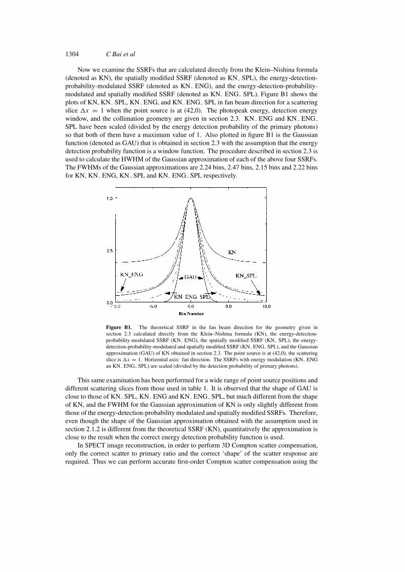
Now we examine the SSRFs that are calculated directly from the Klein–Nishina formula(denoted as KN), the spatially modified SSRF (denoted as KN SPL), the energy-detection-probability-modulated SSRF (denoted as KN ENG), and the energy-detection-probability-modulated and spatially modified SSRF (denoted as KN ENG SPL). Figure B1 shows theplots of KN, KN SPL, KN ENG, and KN ENG SPL in fan beam direction for a scatteringslice �x = 1 when the point source is at (42,0). The photopeak energy, detection energywindow, and the collimation geometry are given in section 2.3. KN ENG and KN ENGSPL have been scaled (divided by the energy detection probability of the primary photons)so that both of them have a maximum value of 1. Also plotted in figure B1 is the Gaussianfunction (denoted as GAU) that is obtained in section 2.3 with the assumption that the energydetection probability function is a window function. The procedure described in section 2.3 isused to calculate the HWHM of the Gaussian approximation of each of the above four SSRFs.The FWHMs of the Gaussian approximations are 2.24 bins, 2.47 bins, 2.15 bins and 2.22 binsfor KN, KN ENG, KN SPL and KN ENG SPL respectively.

Figure B1. The theoretical SSRF in the fan beam direction for the geometry given insection 2.3 calculated directly from the Klein–Nishina formula (KN), the energy-detection-probability-modulated SSRF (KN ENG), the spatially modified SSRF (KN SPL), the energy-detection-probability-modulated and spatially modified SSRF (KN ENG SPL), and the Gaussianapproximation (GAU) of KN obtained in section 2.3. The point source is at (42,0), the scatteringslice is �x = 1. Horizontal axis: fan direction. The SSRFs with energy modulation (KN ENGan KN ENG SPL) are scaled (divided by the detection probability of primary photons).

This same examination has been performed for a wide range of point source positions anddifferent scattering slices from those used in table 1. It is observed that the shape of GAU isclose to those of KN SPL, KN ENG and KN ENG SPL, but much different from the shapeof KN, and the FWHM for the Gaussian approximation of KN is only slightly different fromthose of the energy-detection-probability modulated and spatially modified SSRFs. Therefore,even though the shape of the Gaussian approximation obtained with the assumption used insection 2.1.2 is different from the theoretical SSRF (KN), quantitatively the approximation isclose to the result when the correct energy detection probability function is used.

In SPECT image reconstruction, in order to perform 3D Compton scatter compensation,only the correct scatter to primary ratio and the correct ‘shape’ of the scatter response arerequired. Thus we can perform accurate first-order Compton scatter compensation using the

Blurring model and kernel evaluation for SPECT 1305

proposed model without modelling the energy detection probabilities for either the scatteredphotons or the primary photons. To generate an absolute first-order Compton scatter projectionwe only need to scale the scatter projection obtained using the proposed model by multiplyingby a factor which is the detection probability of the primary photons for the given detectionenergy window.

Acknowledgments

The authors would like to thank Dr John Viner, Dr Wayne Springer, Dr Clayton Williams andDr James Cronin for discussions on the Compton scatter theory. We thank Dr Dan Kadrmasfor his helpful discussions on this paper and thank Paul Christian for arranging the phantomscans. We also thank Sean Webb for editing the manuscript. This work is partially supportedby NIH grant R29 HL51462, HL39792, and a grant from Picker International.

References

Alvarez R E and Macovski A 1976 Energy-selective reconstruction in x-ray computerized tomography Phys. Med.Biol. 21 733–44

Axelsson B, Msaki P and Israelsson A 1984 Subtraction of Compton-scatter photons in single-photon emissioncomputerized tomography J. Nucl. Med. 25 490–4

Bai C, Zeng G L and Gullberg G T 1997 Evaluation of small 2D convolution kernel for slice-by-slice blurring modelof ultra-high-energy collimation (abstract) J. Nucl. Med. 38 214P

——1998b A fan-beam slice-by-slice blurring model for scatter, geometric point response, and attenuation correctionsin SPECT using the iterative OS-EM algorithm (abstract) J. Nucl. Med. 39 120P

Bai C, Zeng G L, Gullberg G T, DiFilippo F and Miller S 1998a Slab-by-slab blurring model for geometric pointresponse correction and attenuation correction using iterative reconstruction algorithm IEEE Trans. Nucl. Sci.45 2168–73

Beekman F J, Eijkman E G J, Viergever M A, Borm G F and Slijpen E T P 1993 Object shape dependent PSF modelfor SPECT imaging IEEE Trans. Nucl. Sci. 40 31–9

Beekman F J, Frey E C, Kamphuis C, Tsui B M W and Viergever M A 1994 A new phantom for fast determinationof scatter response of a Gamma camera IEEE Trans. Nucl. Sci. 41 1481–8

Beekman F J, Kamphuis C and Viergever M A 1996 Improved SPECT quantitation using fully three-dimensionaliterative spatially variant scatter response compensation IEEE Trans. Med. Imaging 15 491–9

Beekman F J, Kamphuis C and Frey E C 1997 Scatter compensation methods in 3 D iterative SPECT reconstruction:a simulation study Phys. Med. Biol. 42 1619–32

Beekman F J and Viergever M A 1995 Fast SPECT simulation including object shape dependent scatter IEEE Trans.Med. Imaging 14 271–82

Bowsher J E and Floyd C E Jr 1991 Treatment of Compton scatter in maximum-likelihood, expectation-maximizationreconstruction of SPECT images J. Nucl. Med. 32 1285–91

Byrne C L 1996 Block-iterative methods for image reconstructing from projections IEEE Trans. Image Proc. 5 792–4Cao Z J, Frey E C and Tsui B M W 1994 A scatter model for parallel and converging beam SPECT based on the

Klein–Nishina formula IEEE Trans. Nucl. Sci. 41 1594–600DeVito R P, Hamill J J, Treffert J D and Stoub T W 1989 Energy-weighted acquisition of scintigraphic images using

finite spatial filters J. Nucl. Med. 30 2029–35Di Bella E V R, Trisjono F and Zeng G L 1996 Recursive blur models for SPECT depth-dependent response (abstract)

J. Nucl. Med. 37 153PFloyd C E, Jaszczak R J and Coleman R E 1985b Inverse Monte Carlo: a unified reconstruction algorithm IEEE Trans.

Nucl. Sci. 32 779–85——1987 Maximum likelihood reconstruction for SPECT with Monte Carlo modeling: asymptotic behavior IEEE

Trans. Nucl. Sci. 34 285–7Floyd C E, Jaszczak R J, Greer K L and Coleman R E 1985a Deconvolution of Compton scatter in SPECT J. Nucl.

Med. 26 403–8——1986 Inverse Monte Carlo as a unified reconstruction algorithm for ECT J. Nucl. Med. 27 1577–85Floyd C E, Jaszczak R J, Harris C C and Coleman R E 1984 Energy and spatial distribution of multiple order Compton

scatter in SPECT: a Monte Carlo investigation Phys. Med. Biol. 29 1217–30

1306 C Bai et al

Formiconi A R, Pupi A and Passeri A 1989 Compensation of spatial system resolution in SPECT with conjugategradient techniques Phys. Med. Biol. 34 69–84

Frey E C, Ju Z W and Tsui B M W 1993 A fast projector–backprojector pair modeling the asymmetric, spatiallyvarying scatter response function for scatter compensation in SPECT imaging IEEE Trans. Nucl. Sci. 40 1192–7

Frey E C and Tsui B M W 1990 Parameterization of the scatter response function in SPECT imaging using MonteCarlo simulation IEEE Trans. Nucl. Sci. 37 1308–15

——1993 A practical method for incorporating scatter in a projector-backprojector for accurate scatter compensationin SPECT IEEE Trans. Nucl. Sci. 40 1107–16

——1994 Modeling the scatter response function in inhomogeneous scattering media for SPECT IEEE Trans. Nucl.Sci. 41 1585–93

——1996 A new method for modeling the spatially-variant, object-dependent scatter response function in SPECTRecord of the 1996 IEEE Nuclear Science Symp. and Medical Imaging Conf. (Piscataway, NJ: IEEE) pp 1082–6

Frey E C, Tsui B M W and Ljungberg 1992 A comparison of scatter compensation methods in SPECT: subtraction-based techniques versus iterative reconstruction with accurate modeling of the scatter Record of the 1992 IEEENuclear Science Symp. and Medical Imaging Conf. (Piscataway, NJ: IEEE) pp 1035–7

Gagnon D, Todd-Pokropek A E, Arsenault A and Dupras G 1989 Introduction to holospectral imaging in nuclearmedicine for scatter subtraction IEEE Trans. Med. Imaging 8 245–50

Gilland D R, Jaszczak R J, Wang H, Turkington T G, Greer K L and Coleman R E 1994 Approximate 3D iterativereconstruction for SPECT Phys. Med. Biol. 39 547–61

Halama J R, Henkin R E and Friend L E 1988 Gamma camera radionuclide images: improved contrast with energy-weighted acquisition Radiology 169 533–8

Hamill J J and Devito R P 1989 Scatter reduction with energy weighted acquisition IEEE Trans. Nucl. Sci. 36 1334–9Hudson H M and Larkin R S 1994 Accelerated image reconstruction using ordered subsets of projection data IEEE

Trans. Med. Imaging 13 601–9Hutton B F 1997 Cardiac single-photon emission tomography: is attenuation correction enough? Eur. J. Nucl. Med.

24 713–5Hutton B F, Osiecki A and Meikle S R 1996 Transmission-based scatter correction of 180 degrees myocardial single-

photon emission tomographic studies Eur. J. Nucl. Med. 23 1300–8Jaszczak R J, Floyd C E and Coleman R E 1985 Scatter compensation techniques for SPECT IEEE Trans. Nucl. Sci.

32 786–93Jaszcak R J, Greer K L, Floyd C E, Harris C C and Coleman R E 1984 Improved SPECT quantification using

compensation for scattered photons J. Nucl. Med. 25 893–900Johns H E and Cunningham J R 1974 The Physics of Radiology 3rd edn (Springfield, IL: Charles C Thomas) p 175Ju Z W, Frey E C and Tsui B M W 1995 Distributed 3-D iterative reconstruction for quantitative SPECT IEEE Trans.

Nucl. Sci. 42 1301–9Kadrmas D J, Frey E C, Karimi S S and Tsui B M W 1998 Fast implementation of reconstruction-based scatter

compensation in fully 3D SPECT image reconstruction Phys. Med. Biol. 43 857–73Kadrmas D J, Frey E C and Tsui B M W 1996 An SVD investigation of modeling scatter in multiple energy windows

for improved SPECT images IEEE Trans. Nucl. Sci. 43 2275–84——1997 Analysis of the reconstructibility and noise properties of scattered photons in 99mTc SPECT Phys. Med.

Biol. 42 2493–516Kamphuis C, Beekman F J, Rijk P P and Viergever M A 1998 Dual matrix ordered subsets reconstruction for accelerated

3D scatter compensation in single-photon emission tomography Eur. J. Nucl. Med. 25 8–18King M A, Hademenos G J and Glick S J 1992 A dual-photopeak window method for scatter correction J. Nucl. Med.

33 605–12Klein O and Nishina Y 1928 Uber die streuung von strahlung durch freielektronen nach der neuen relativistischen

quantendynamik von Dirac Z. Physik 52 853–68Koral K F, Swailem F M, Buchbinder S, Clinthorne N H, Rogers W L and Tsui B M W 1990 SPECT dual-energy-

window Compton correction: scatter multiplier required for quantification J. Nucl. Med. 31 90–8Koral K F, Wang X, Rogers W L, Clinthorne N H and Wang X 1988 SPECT Compton-scattering correction by analysis

of energy spectra J. Nucl. Med. 29 195–202Laurette I, Zeng G L and Gullberg G T 1999 A three-dimensional ray-tracing method to correct for non-uniform

attenuation, scatter, and detector response in SPECT Proc. 1999 International Meeting on Fully Three-Dimensional Image Reconstruction in Radiology and Nuclear Medicine (Egmond aan Zee, The Netherlands,June 23–26, 1999) ed F Beekman, M Defrise and M Viergever, pp 145–8

Lowry C A and Cooper M J 1987 The problem of Compton scattering in emission tomography: a measurement of itsspatial distribution Phys. Med. Biol. 32 1187–91

McCarthy A W and Miller M I 1991 Maximum likelihood SPECT in clinical computation times using mesh-connected

Blurring model and kernel evaluation for SPECT 1307

parallel computers IEEE Trans. Med. Imaging 10 426–36Meikle S R, Hutton B F and Bailey D L 1994 A transmission-dependent method for scatter correction in SPECT

J. Nucl. Med. 35 360–7Msaki P, Axelsson B, Dahl C M and Larsson S A 1987 Generalized scatter correction method in SPECT using point

scatter distribution functions J. Nucl. Med. 28 1861–9Msaki P, Axelsson B and Larsson S A 1989 Some physical factors influencing the accuracy of convolution scatter

correction in SPECT Phys. Med. Biol. 34 283–98Ogawa K, Harata Y, Ichihara T, Kubo A and Hashimoto S 1991 A practical method for position-dependent Compton-

scatter correction in single photon emission CT IEEE Trans. Med. Imaging 10 408–12Phelps M E, Hoffman E J and Ter-Pogossian M M 1975 Attenuation coefficients of various body tissues, fluids, and

lesions at photon energies of 18 to 136 keV Radiology 117 573–83Riauka T A and Gortel Z W 1994 Photon propagation and detection in single-photon emission computed tomography:

an analytical approach Med. Phys. 21 1311–22Riauka T A, Hooper H R and Gortel Z W 1996 Experimental and numerical investigation of the 3D SPECT photon

detection kernel for non-uniform attenuating media Phys. Med. Biol. 41 1167–89Sorenson J A and Phelps M E 1987 Physics in Nuclear Medicine 2nd edn (Orlando, FL: Grune & Stratton) p 188Terry J A, Tsui B M W, Perry J R, Hendricks J L and Gullberg G T 1990 The design of a mathematical phantom of

the upper human torso for use in 3-D SPECT imaging research Biomedical Engineering: Opening New Doors,Proc. 1990 Fall Meeting of the Biomedical Engineering Soc. (Blacksburg, VA) (Blacksburg, VA: New YorkUniversity Press) pp 1467–74

Tsui B M W, Frey E C, Zhao X D, Lalush D S, Johnston R E and McCartney W H 1994 The importance andimplementation of accurate 3-D compensation methods for quantitative SPECT Phys. Med. Biol. 39 509–30

Tsui B M W, Gullberg G T, Edgerton E R, Ballard J G, Perry J R, McCartney W H and Berg J 1989 Correction ofnonuniform attenuation in cardiac SPECT imaging J. Nucl. Med. 28 497–507

Tsui B M W, Hu H D, Gilland D R and Gullberg G T 1988 Implementation of simultaneous attenuation and detectorresponse correction in SPECT IEEE Trans. Nucl. Sci. 35 778–83

Vannoy S 1994 The Photon History Generator release 2.5b (University of Washington Medical Center)Veklerov E, Llacer J and Hoffman E 1988 MLE reconstruction of a brain phantom using a Monte Carlo transition

matrix and a statistical stopping rule IEEE Trans. Nucl. Sci. 35 603–7Wallis J W, Miller T R, Miller M M and Hamill J 1996 Rapid 3-D projection in iterative reconstruction using Gaussian

diffusion (abstract) J. Nucl. Med. 37 63PWalrand S, Elmbt L and Pauwels S 1994 Quantification of SPECT using an effective model of the scattering Phys.

Med. Biol. 39 719–34Welch A and Gullberg G T 1996 Acceleration of a model based scatter correction scheme for SPECT by use of an

unmatched project-backprojector Record IEEE Nucl. Sci. Symp. (California, 1996) (New York: IEEE) pp 1072–6——1997 Implementation of a model-based non-uniform scatter correction scheme for SPECT IEEE Trans. Med.

Imaging 16 717–26Welch A, Gullberg G T, Christian P E and Datz F L 1995 A transmission-map-based scatter correction technique for

SPECT in inhomogeneous media Med. Phys. 22 1627–35Wells R G, Celler A and Harrop R 1997 Experimental validation of an analytical method of calculating SPECT

projection data IEEE Trans. Nucl. Sci. 44 1283–90——1998 Analytical calculation of photon distributions in SPECT projections IEEE Trans. Nucl. Sci. 45 3202–14Zeng G L, Bai C and Gullberg G T 1999 A projector/backprojector with slice-to-slice blurring for efficient 3D scatter

modeling IEEE Trans. Med. Imaging 18 722–32Zeng G L and Gullberg G T 1996 Valid backprojection matrices which are not the transpose of the projection matrix

(abstract) J. Nucl. Med. 37 206P——1997 On using an unmatched projector and backprojector pair in an iterative algorithm (abstract) J. Nucl. Med.

38 58P——2000 Unmatched projector/backprojector pairs in an iterative reconstruction algorithm IEEE Trans. Med. Imaging

at pressZeng G L, Gullberg G T, Bai C, Christian P E, Trisjono F, DiBella E V R, Tanner J W and Morgan H T 1998 Iterative

reconstruction of fluorine-18 SPECT using geometric point response correction J. Nucl. Med. 39 124–30Zeng G L, Gullberg G T, Tsui B M W and Terry J A 1991 Three-dimensional iterative reconstruction algorithms with

attenuation and geometric point response correction IEEE Trans. Nucl. Sci. 38 693–702Zeng G L, Hsieh Y L and Gullberg G T 1994 A rotating and warping projector/backprojector for fan-beam and

cone-beam iterative algorithm IEEE Trans. Nucl. Sci. 41 2807–11