A Simultaneous Confidence Corridor for Varying - SFB 649

S F

B XXX

E

C O

N O

M I

C

R I

S K

B

E R

L I

N

SFB 649 Discussion Paper 2014-002

A Simultaneous Confidence Corridor for

Varying Coefficient

Regression with Sparse Functional Data

Lijie Gu*

Li Wang**

Wolfgang Karl Härdle*** Lijian Yang*/****

* Soochow University, China

** University of Georgia, USA

*** Humboldt-Universität zu Berlin, Germany **** Michigan State University, USA

This research was supported by the Deutsche

Forschungsgemeinschaft through the SFB 649 "Economic Risk".

http://sfb649.wiwi.hu-berlin.de

ISSN 1860-5664

SFB 649, Humboldt-Universität zu Berlin Spandauer Straße 1, D-10178 Berlin

SFB

6

4 9

E

C O

N O

M I

C

R I

S K

B

E R

L I

N

A Simultaneous Confidence Corridor for Varying

Coefficient Regression with Sparse Functional Data

1

Lijie Gu

Center for Advanced Statistics and Econometrics Research

Soochow University

Suzhou 215006, China email: [email protected]

Li Wang

Department of Statistics

University of Georgia

Athens, GA 30602 email: [email protected]

Wolfgang K. Hardle

C.A.S.E. – Center for Applied Statistics and Economics

Humboldt-Universitat zu Berlin

Unter den Linden 6

10099 Berlin, Germany email: [email protected]

and

Lee Kong Chian School of Business, Singapore Management University

Lijian Yang

Center for Advanced Statistics and Econometrics Research

Soochow University

Suzhou 215006, China email: [email protected]

and

Department of Statistics and Probability

Michigan State University

East Lansing, MI 48824 email: [email protected]

Author’s Footnote:

Lijie Gu is Ph.D. student, Center for Advanced Statistics and Econometrics Research,

Soochow University, Suzhou 215006, China (E-mail: [email protected]). Li Wang is

Associate Professor, Department of Statistics, University of Georgia, Athens, GA 30602

(E-mail: [email protected]). Wolfgang K. Hardle is Professor, C.A.S.E. – Center for Ap-

plied Statistics and Economics, Humboldt-Universitat zu Berlin, Unter den Linden 6, 10099

Berlin, Germany, and Distinguished Visiting Professor, Lee Kong Chian School of Busi-

ness, Singapore Management University (E-mail: [email protected]). Lijian

Yang is Director, Center for Advanced Statistics and Econometrics Research, Soochow U-

niversity, Suzhou 215006, China, and Professor, Department of Statistics and Probability,

Michigan State University, East Lansing, MI 48824 (E-mail: [email protected];

[email protected]). This work is supported in part by the Deutsche Forschungsgemein-

schaft through the CRC 649 “Economic Risk”, the US National Science Foundation awards

DMS 0905730, 1007594, 1106816, 1309800, Jiangsu Specially-Appointed Professor Program

SR10700111, Jiangsu Province Key-Discipline Program (Statistics) ZY107002, National Nat-

ural Science Foundation of China award 11371272, and Research Fund for the Doctoral

Program of Higher Education of China award 20133201110002.

3

Abstract

We consider a varying coefficient regression model for sparse functional data, with time

varying response variable depending linearly on some time independent covariates with co-

efficients as functions of time dependent covariates. Based on spline smoothing, we propose

data driven simultaneous confidence corridors for the coefficient functions with asymptoti-

cally correct confidence level. Such confidence corridors are useful benchmarks for statistical

inference on the global shapes of coefficient functions under any hypotheses. Simulation

experiments corroborate with the theoretical results. An example in CD4/HIV study is used

to illustrate how inference is made with computable p-values on the effects of smoking, pre-

infection CD4 cell percentage and age on the CD4 cell percentage of HIV infected patients

under treatment.

Keywords: B spline, confidence corridor, Karhunen-Loeve L2 representation, knots, func-

tional data, varying coefficient.

JEL Classification: C14, C23

4

1. INTRODUCTION

Functional data are commonly encountered in biomedical studies, epidemiology and social

science, where information is collected over a time period for each subject. In many longitu-

dinal studies, repeated measurements are often collected at few irregular time points. Data

of this type are frequently referred to as sparse longitudinal or sparse functional data. See,

for example, James, Hastie and Sugar (2000), James and Sugar (2003), Yao, Muller and

Wang (2005a), Hall, Muller and Wang (2006), and Zhou, Huang and Carroll (2008).

In longitudinal study, often, interest lies in studying the association between the co-

variates and the response variable. In recent years, there has been an increasing interest

in nonparametric analysis of longitudinal data to enhance flexibility, see e.g., Yao and Li

(2013). The varying coefficient model (VCM) proposed by Hastie and Tibshirani (1993)

strikes a delicate balance between the simplicity of linear regression and the flexibility of

multivariate nonparametric regression and has been widely applied in various settings, for

instance, the Cobb-Douglas model for GDP growth in Liu and Yang (2010), and the longi-

tudinal model for CD4 cell percentages in AIDS patients in Wu and Chiang (2000), Fan and

Zhang (2000) and Wang, Li and Huang (2008). See Fan and Zhang (2008) for an extensive

literature review of VCM.

To examine whether the association changes over time, Hoover et al. (1998) proposed

the following varying coefficient model

Y (t) = β0(t) +X(t)Tβ(t) + ε(t), t ∈ T , (1)

where X(t) = (X1(t), . . . , Xd(t))T are covariates at time t, β(t) = (β1(t), . . . , βd(t))

T are

functions of t, and ε(t) is a mean zero process. Model (1) is a special case of functional

linear models, see Ramsay and Silverman (2005) and Wu, Fan and Muller (2010).

The coefficient functions βl(t)’s in model (1) can be estimated by, for example, kernel

method in Hoover et al. (1998), basis function approximation method in Huang, Wu and

Zhou (2002), polynomial spline method in Huang, Wu and Zhou (2004) and smoothing spline

method in Brumback and Rice (1998). Fan and Zhang (2000) proposed a two-step method

5

to overcome the computational burden of the smoothing spline method.

For some longitudinal studies, the covariates are independent of time, and their observa-

tions are cross-sectional. Take for instance the longitudinal CD4 cell percentage data among

HIV seroconverters. This dataset contains 1817 observations of CD4 cell percentages on 283

homosexual men infected with the HIV virus. Three of the covariates are observed at the

time of HIV infection and hence by nature independent of the measurement time and fre-

quency: Xi1, the i-th patient’s smoking status; Xi2, the i-th patient’s centered pre-infection

CD4 percentage; and Xi3 the i-th patient’s centered age at the time of HIV infection. A

fourth predictor, however, is time dependent: Tij, the time (in years) of the j-th measure-

ment of CD4 cell on the i-th patient after HIV infection; while the response Yij is also time

dependent: the j-th measurement of the i-th patient’s CD4 cell percentage at time Tij.

Wu and Chiang (2000), Fan and Zhang (2000) and Wang, Li and Huang (2008) all contain

detailed descriptions and analysis of this dataset.

A feasible VCM for multivariate functional data such as the above takes the form

Yij =d∑

l=1

ηil (Tij)Xil + σ (Tij) εij, 1 ≤ i ≤ n, 1 ≤ j ≤ Ni, (2)

where the measurement errors (εij)n,Ni

i=1,j=1 satisfy E (εij) = 0, E(ε2ij) = 1, and ηil(t), t ∈ T

are i.i.d copies of a L2 process ηl(t), t ∈ T , i.e., E∫T η

2l (t)dt < +∞, l = 1, . . . , d. The com-

mon mean function of processes ηl(t), t ∈ T is denoted as ml(t) = Eηl(t), l = 1, . . . , d.

The actual data set consists of Xi, Tij, Yij, 1 ≤ i ≤ n, 1 ≤ j ≤ Ni, in which the i-th subject

is observed Ni times, the time independent covariates for the i-th subject are Xi = (Xil)dl=1,

1 ≤ i ≤ n, and the random measurement time Tij ∈ T = [a, b]. The aforementioned data

example is called sparse functional as the number of measurements Ni for the i-th subject

is relatively low. (In the above CD4 example actually at most 14). In contrast, for a dense

functional data limn→∞ min1≤i≤nNi = ∞.

For the CD4 cell percentage data, we introduce a fourth time independent covariate, the

baseline Xi0 ≡ 1, and denote by ml (t), l = 0, 1, 2, 3, the coefficient functions for baseline

CD4 percentage, smoking status, centered pre-infection CD4 percentage and centered age,

6

respectively. Figures 2-5 contain spline estimates of the ml (t), 0 ≤ l ≤ 3, and simultaneous

confidence corridors (SCC) at various confidence levels.

In previous works the theoretical focus has mainly been on consistency and asymptotic

normality of the estimators of the coefficient functions of interest, and the construction of

pointwise confidence intervals. However, as demonstrated in Fan and Zhang (2000), this

is unsatisfactory as investigators are often interested in testing whether some coefficient

functions are significantly nonzero or varying, for which a SCC is needed. Take for instance,

Figure 3, which shows both the 95% and 20.277% SCC of m1 (t) contain the zero line

completely, thus with a very high p-value of 0.79723 the null hypothesis of m1 (t) ≡ 0, t ∈ T

is not rejected. More details are in Section 6.

Construction of computationally simple SCCs with exact coverage probability is known

to be difficult even with independent cross-sectional data; see, Wang and Yang (2009) and re-

lated earlier work Hardle and Luckhaus (1984) on uniform consistency. Most earlier methods

proposed in the literature restrict to asymptotic conservative SCCs. Wu, Chiang and Hoover

(1998) developed asymptotic SCCs for the unknown coefficients based on local polynomial

methods, which are computationally intensive, as the kernel estimator requires solving an

optimization problem at every point. Huang, Wu and Zhou (2004) proposed approximating

each coefficient function by a polynomial spline and developed spline SCCs, which are simpler

to construct, while Xue and Zhu (2007) proposed maximum empirical likelihood estimators

and constructed SCCs for the coefficient functions. All these SCCs are Bonferroni-type vari-

ability bands according to Hall and Titterington (1988). The idea is to invoke pointwise

confidence intervals on a very fine grid of [a, b], then adjust the level of these confidence

intervals by the Bonferroni method to obtain uniform confidence bands, and finally bridge

the gaps between the grid points via smoothness conditions on the coefficient curve. How-

ever, to use these bands in practice, one must have a priori bounds on the magnitude of

the bias on each subinterval as well as a choice for the number of grid points. Chiang, Rice

and Wu (2001) proposed a bootstrap procedure to construct confidence intervals. However,

theoretical properties of their procedures have not yet been developed.

7

In this paper, we derive SCCs with exact coverage probability for the coefficient functions

ml(t), l = 1, . . . , d, in (3) via extreme value theory of Gaussian processes and approximating

coefficient functions by piecewise-constant splines. The results represent the first attempt at

developing exact SCCs for the coefficient functions in VCM for sparse functional data. Our

simulation studies indicate the proposed SCCs are computationally efficient and have the

right coverage probability for finite samples. Our work parallels Zhu, Li and Kong (2012)

which established asymptotic theory of SCC in the case of VCM for dense functional data.

It is important to mention as well that the linear covariates in Zhu, Li and Kong (2012)

are time dependent, which does not complicate the problem as they work with dense data

instead of the sparse data we concentrate on.

We organize our paper as follows. Section 2 describes spline estimators, and establish

their asymptotic properties for sparse longitudinal data. Section 3.1 proposes asymptotic

pointwise confidence intervals and SCCs constructed from piecewise constant splines. Section

3.2 describes actual steps to implement the proposed SCCs. In Section 4 we provide further

insights into the estimation error structure of spline estimators. Section 5 reports findings

from a simulation study. A real data example appears in Section 6. Proofs of technical

lemmas are in the Appendix and Supplementary Materials.

2. SPLINE ESTIMATION AND ASYMPTOTIC PROPERTIES

For a functional data Xi, Tij, Yij, 1 ≤ i ≤ n, 1 ≤ j ≤ Ni, denote the eigenvalues and

eigenfunctions sequences of its covariance operator Gl (s, t) = cov ηl(s), ηl(t) as λk,l∞k=1,ψk,l(t)

∞k=1

, in which λ1,l ≥ λ2,l ≥ · · · ≥ 0,∑∞

k=1 λk,l <∞, andψk,l

∞k=1

form an orthonor-

mal basis of L2 (T ). It follows from spectral theory that Gl (s, t) =∑∞

k=1 λk,lψk,l(s)ψk,l (t).

For any l = 1, . . . , d, the i-th trajectory ηil(t), t ∈ T allows the Karhunen-Loeve L2 rep-

resentation (Yao, Muller and Wang, 2005b): ηil(t) = ml(t) +∑∞

k=1 ξik,lϕk,l(t), where the

random coefficients ξik,l are uncorrelated with mean 0 and variances 1, and the functions

ϕk,l =√λk,lψk,l, thus Gl(s, t) =

∑∞k=1 ϕk,l(s)ϕk,l (t), and the response measurements (2) can

8

be represented as follows

Yij =d∑

l=1

ml (Tij)Xil +d∑

l=1

∞∑k=1

ξik,lϕk,l (Tij)Xil + σ (Tij) εij. (3)

Without loss of generality, we take T = [a, b] to be [0, 1]. Following Xue and Yang (2006),

we approximate each coefficient function by the spline smoothing method. To describe the

spline functions, one can divide the finite interval [0, 1] into (Ns + 1) equal subintervals

χJ = [υJ , υJ+1), J = 0, . . . , Ns − 1, χNs= [υNs , 1]. A sequence of equally-spaced points

υJNs

J=1, called interior knots, are given as υ0 = 0 < υ1 < · · · < υNs < 1 = υNs+1. Let

υJ = Jhs for 0 ≤ J ≤ Ns + 1, where hs = 1/ (Ns + 1) is the distance between neighboring

knots. We denote by G(−1) = G(−1) [0, 1] the space of functions that are constant on each

subinterval χJ , and the B-spline basis of G(−1), as bJ(t)Ns

J=0, which are simply indicator

functions of intervals χJ , bJ(t) = IχJ(t), J = 0, 1, . . . , Ns. For any t ∈ [0, 1], define its

location index as J(t) = Jn(t) = min [t/hs] , Ns so that t ∈ χJ(t).

Next we define the space of spline coefficient functions on T × Rd as

M =

g (t,x) =

d∑l=1

gl(t)xl : gl(t) ∈ G(−1), t ∈ T ,x = (x1, . . . , xd)T ∈ Rd

,

and propose estimating the multivariate function∑d

l=1ml(t)xl by

m (t,x) =d∑

l=1

ml(t)xl = argming∈M

n∑i=1

Ni∑j=1

Yij − g (Tij,Xi)2 . (4)

Let σ2Y (t,x) be the conditional variance ofY given T = t andX = x = (x1, . . . , xd)

T ∈ Rd

σ2Y (t,x) = Var(Y |T = t,X = x) =

d∑l=1

Gl (t, t) x2l + σ2(t).

Next for any t ∈ [0, 1], let

Γn(t) = c−2J(t),nnE(N1)−1 EXXT

[∫χJ(t)

σ2Y (u,X) f (u) du (5)

+E N1(N1 − 1)

EN1

∑d

l=1X2

l

∫χJ(t)×χJ(t)

Gl (u, v) f (u) f (v) dudv

],

9

where

cJ,n = E b2J(T ) =

∫ 1

0

b2J(t)f(t)dt, J = 0, . . . , Ns. (6)

Further denote

Σn(t) = H−1Γn(t)H−1 =

σ2n,ll′(t)

dl,l′=1

, (7)

where σ2n,ll′(t) are later shown to be the asymptotic covariances between ml(t) and ml′(t).

Theorem 1. Under Assumptions (A1)–(A6) in Appendix A, for any t ∈ [0, 1], as n→ ∞,

Σ−1/2n (t) m(t)−m (t) L−→ N (0, Id×d) ,

where m(t) = (m1(t), . . . , md(t))T is the estimate of m(t) = (m1(t), . . . ,md(t))

T. Further-

more, for any l = 1, . . . , d and α ∈ (0, 1),

limn→∞

Pσ−1n,ll(t) |ml(t)−ml(t)| ≤ Z1−α/2

= 1− α.

Remark 1. Note that Σn(t) =σ2n,ll′(t)

dl,l′=1

in (7) is complicated to compute in practice.

The next proposition suggests that, for any t ∈ [0, 1], Γn(t) in (5) can be simplified by

Γn(t) ≡ E

[XXT σ2

Y (t,X)

f(t)hsnE(N1)

1 +

EN1 (N1 − 1)

EN1

∑dl=1X

2l Gl (t, t) f(t)hsσ2Y (t,X)

]. (8)

Denote the supremum norm of a function ϕ on [a, b] by ∥ϕ∥∞ = supt∈[a,b] |ϕ(t)|. For

any matrix A = (aij), define ∥A∥∞ = max |aij|, where the maximum is taken over all the

elements of A, while for a matrix function A(t) = (aij(t)), ∥A∥∞ = supt∈[a,b] ∥A(t)∥∞.

Proposition 1. Under Assumptions (A2)–(A6) in Appendix A, there exists a constant

c > 0 such that as n→ ∞, ∥Γn(t)− Γn(t)∥∞ = O (n−1hr−1s ) = O (n−c) .

To derive the maximal deviation distribution of estimators ml(t), l = 1, . . . , d, let

QNs+1 (α) = bNs+1 − a−1Ns+1 log

−1

2log(1− α)

, α ∈ (0, 1) (9)

aNs+1 = 2 log (Ns + 1)1/2 , bNs+1 = aNs+1 −log(2πa2Ns+1

)2aNs+1

. (10)

10

Theorem 2. Under Assumptions (A1)–(A6) in Appendix A, for l = 1, . . . , d and any α ∈

(0, 1),

limn→∞

P

supt∈[0,1]

σ−1n,ll(t) |ml(t)−ml(t)| ≤ QNs+1 (α)

= 1− α,

where σn,ll(t) and QNs+1 (α) are given in (7) and (9), respectively.

3. ASYMPTOTIC CONFIDENCE REGIONS

In this section we construct the confidence regions for functions ml(t), l = 1, . . . , d.

3.1 Asymptotic Confidence Intervals and SCCs

Theorems 1 and 2 allow one to construct pointwise confidence intervals and SCCs for com-

ponents ml(t), l = 1, . . . , d. The next corollary provides the theoretical underpinning upon

which SCCs can be actually implemented, see subsection 3.2.

Corollary 1. Under Assumptions (A1)-(A6) in Appendix A, for any l = 1, . . . , d and

α ∈ (0, 1), as n→ ∞,

(i) an asymptotic 100 (1− α)% pointwise confidence interval forml(t), t ∈ [0, 1], is ml(t)±

σn,ll(t)Z1−α/2, with σn,ll(t) given in (7), while Z1−α/2 is the 100 (1− α/2)th percentile

of the standard normal distribution.

(ii) an asymptotic 100 (1− α)% SCC for ml(t), with QNs+1 (α) given in (9), is ml(t) ±

σn,ll(t)QNs+1 (α), t ∈ [0, 1].

3.2 Implementation

In the following we describe procedures to construct the SCCs and the pointwise intervals

given in Corollary 1. For any data set (Tij, Yij, Xil)n,Ni,di=1,j=1,l=1 from model (3), the spline

estimators ml(t), l = 1, . . . , d, are obtained by (4), and the number of interior knots is taken

to be Ns = [cN1/3T (log(n))], in which NT =

∑ni=1Ni is the total sample size, [a] denotes the

integer part of a, and c is a positive constant.

11

To construct the SCCs, one needs to evaluate the functions σ2n,ll(t), l = 1, . . . , d, which

are the diagonal elements of matrix Σn(t) in (7). Based on Proposition 1, one can estimate

each unknowns f(t), σ2Y (t,x), Gl (t, t) and matrix H and then plug these estimators into the

formula of the SCCs; see Wang and Yang (2009).

The number of interior knots for pilot estimation of f(t), σ2Y (t,x), and Gl (t, t) is taken

to be N∗s =

[0.5n1/3

], and h∗s = 1/ (1 +N∗

s ). The histogram pilot estimator of the density

function f(t) is f(t) = N−1T h∗−1

s

∑ni=1

∑Ni

j=1 bJ(t)(Tij).

We now discuss the estimation of Γn (t) in (5). Defining Rij =(Yij −

∑dl=1 m(Tij)Xil

)2,

1 ≤ j ≤ Ni, 1 ≤ i ≤ n, the estimator of σ2Y (t,x) is

σ2Y (t,x) =

d∑l=1

N∗s∑

J=0

ρJ,lbJ(t)x2l +

N∗s∑

J=0

µJbJ(t) =d∑

l=1

Gl (t, t)x2l + σ2(t),

where ρ0,1, . . . , ρN∗s ,d, µ0, . . . , µN∗

sT are solutions of the following least squares problem:

(ρ0,1, . . . , ρN∗

s ,d, µ0, . . . , µN∗

s

)T=

argmin

(ρ0,1,...,µN∗s )

T∈R(N∗

s +1)(d+1)

n∑i=1

Ni∑j=1

Rij −

d∑l=1

N∗s∑

J=0

ρJ,lbJ(Tij)X2il −

N∗s∑

J=0

µJbJ(Tij)

2

.

The matrix Γn (t) is estimated by substituting f(t), Gl (t, t) and σ2Y (t,x) with f(t), Gl (t, t)

and σ2Y (t,x). Define

Γn (t) ≡

[n−1

n∑i=1

XilXil′σ2Y (t,Xi)

f(t)hsNT

−1

×

1 +

(∑ni=1N

2i

NT

− 1

)∑dl=1 Gl (t, t)X

2il

σ2Y (t,Xi)

f(t)hs

]dl,l′=1

.

The following proposition provides the consistent rate of Γn(t) to Γn(t).

Proposition 2. Under Assumptions (A1)-(A6) in Appendix A, there exists a constant c > 0

such that as n→ ∞,∥∥∥Γn(t)− Γn(t)

∥∥∥∞

= Op (n−c).

Proposition 2 implies that Γn(t) can be replaced by Γn(t) with a negligible error. Define

a d × d matrix H = n−1∑n

i=1XilXil′dl,l′=1, then Σn(t) can be estimated well by Σn(t) =

12

σ2n,ll′(t)

dl,l′=1

= H−1Γn (t) H−1. Therefore, as n→ ∞, l = 1, . . . , d, the SCCs

ml(t)± σn,ll(t)QNs+1 (α) , (11)

with QNs+1 (α) given in (9), and the pointwise intervals ml(t)±σn,ll(t)Z1−α/2 have asymptotic

confidence level 1− α.

4. DECOMPOSITION

In this section, we describe the representation of the spline estimators ml(t), l = 1, . . . , d,

in (4), then break the estimation error ml(t)−ml(t) into three terms by the decomposition

of Yij in model (3). Although such representation is not needed for applying the procedure

describe in Section 3.2 to analyze data, it sheds insights into the proof of the main theoretical

results in Section 2.

We consider the following rescaled B-spline basis BJ(t)Ns

J=0 for G(−1):

BJ(t) ≡ bJ(t) (cJ,n)−1/2 , J = 0, . . . , Ns. (12)

It is easily verified that EBJ(T )2 = 1 for J = 0, 1, . . . , Ns, and BJ(t)BJ ′(t) ≡ 0 for J = J ′.

By simple linear algebra, the spline estimator ml(t) defined in (4) equals

ml(t) =Ns∑J=0

γJ,lBJ(t) = c−1/2J(t),nγJ(t),l , l = 1, . . . , d, (13)

where the coefficients γ =(γT0 , . . . , γ

TNs

)Twith γJ =

(γJ,1, . . . , γJ,d

)Tbeing the solution of

the following least squares problem

γ = argmin

γ=(γ0,1,...,γNs,d)T∈Rd(Ns+1)

n∑i=1

Ni∑j=1

Yij −

d∑l=1

Ns∑J=0

γJ,lBJ (Tij)Xil

2

. (14)

In the following let Y = (Y11, . . . , Y1N1 , . . . , Yn1, . . . , YnNn)T be the collection of all the

Yij’s. Let B(t) = (B0(t), . . . , BNs(t))T and Xi = (Xi1, . . . , Xid)

T be two vectors of dimension

(Ns + 1) and d, respectively. Denote

D = (B(T11)⊗X1, . . . ,B(T1N1)⊗X1, . . . ,B(Tn1)⊗Xn, . . . ,B(TnNn)⊗Xn)T , (15)

13

a NT × ((Ns + 1) d) matrix, where “⊗” denotes the Kronecker product. Solving the least

squares problem in (14), we obtain

γ =(DTD

)−1 (DTY

). (16)

Denote x = (x1, . . . , xd)T, thus equation (4) can be rewritten as

d∑l=1

ml(t)xl = (B(t)⊗ x)T(DTD

)−1 (DTY

). (17)

According to (15), one has DTD =∑n

i=1

∑Ni

j=1

B(Tij)B(Tij)

T ⊗XiXTi

, in which ma-

trix B(Tij)B(Tij)T = diag

B2

0(Tij), . . . , B2Ns(Tij)

. So matrix DTD should be a block diag-

onal matrix, and we write N−1T DTD = diag V0, . . . , VNs, where

VJ =

N−1

T

n∑i=1

Ni∑j=1

B2J(Tij)XilXil′

d

l,l′=1

. (18)

On the other hand, we haveDTY =∑n

i=1

∑Ni

j=1 B(Tij)⊗XiYij. Thus, γ =(γT0 , . . . , γ

TNs

)Tcan be easily calculated using

γJ = V−1J

N−1

T

n∑i=1

Ni∑j=1

BJ(Tij)XilYij

d

l=1

, J = 0, . . . , Ns. (19)

Then the functions m(t) = (m1(t), . . . ,md(t))T can be simply estimated by

m(t) = (m1(t), . . . , md(t))T = c

−1/2J(t),n

(γJ(t),1, . . . , γJ(t),d

)T= c

−1/2J(t),nγJ(t). (20)

Projecting the relationship in model (3) onto the space of spline coefficient functions on

T ×Rd as M, we obtain the following important decomposition:

d∑l=1

ml(t)xl =d∑

l=1

ml(t)xl +d∑

l=1

ξl(t)xl +d∑

l=1

εl(t)xl, (21)

where for any l = 1, . . . , d,

ml(t) =Ns∑J=0

γJ,lBJ(t) = c−1/2J(t),nγJ(t),l, (22)

14

ξl(t) =Ns∑J=0

αJ,lBJ(t) = c−1/2J(t),nαJ(t),l, εl(t) =

Ns∑J=0

θJ,lBJ(t) = c−1/2J(t),nθJ(t),l, (23)

and the vectors (γJ,l, J = 0, . . . , Ns, l = 1, . . . , d)T, (αJ,l, J = 0, . . . , Ns, l = 1, . . . , d)T, and

(θJ,l, J = 0, . . . , Ns, l = 1, . . . , d)T are solutions to (14) with Yij replaced by∑d

l=1ml (Tij)Xil,∑dl=1

∑∞k=1 ξik,lϕk,l (Tij)Xil, and σ (Tij) εij, respectively.

Furthermore, under Assumption (A5) we can decompose ml(t) as

ml(t) = ml(t) + ξl(t) + εl(t), l = 1, . . . , d. (24)

The next two propositions concern the functions ml(t), ξl(t), εl(t), l = 1, . . . , d, given in

(22) and (23). Proposition 3 gives the uniform convergence rate of ml(t) toml(t). Proposition

4 provides the asymptotic distribution for the maximum of the normalized error terms.

Proposition 3. Under Assumptions (A1), (A2) and (A4)–(A6) in Appendix A, the func-

tions ml(t), l = 1, . . . , d satisfy supt∈[0,1] sup1≤l≤d |ml(t)−ml(t)| = Op(hs).

Proposition 4. Under Assumptions (A2)–(A6) in Appendix A, for τ ∈ R, and σn,ll(t),

aNs+1, bNs+1 as given in (7) and (9),

limn→∞

P

supt∈[0,1]

σ−1n,ll(t)

∣∣∣ξl(t) + εl(t)∣∣∣ ≤ τ/aNs+1 + bNs+1

= exp

(−2e−τ

).

5. SIMULATION

To illustrate the finite-sample performance of the spline approach, we generate data from

the following model

Yij =

m1 (Tij) +

2∑k=1

ξik,1ϕk,1 (Tij)

Xi1 +

m2 (Tij) +

3∑k=1

ξik,2ϕk,2 (Tij)

Xi2

+σ (Tij) εij, 1 ≤ i ≤ n, 1 ≤ j ≤ Ni,

where T ∼ U [0, 1], X1 ∼ N(0, 1), X2 ∼ Binomial[1, 0.5], ξk,1 ∼ N(0, 1), k = 1, 2, ξk,2 ∼

N(0, 1), k = 1, 2, 3, ε ∼ N(0, 1), and Ni is generated from a discrete uniform distribution

from 2, . . . , 14, for 1 ≤ i ≤ n. For the first component, we take m1(t) = sin 2π (t− 1/2),

15

ϕ1,1(t) = −2 cos π (t− 1/2) /√5, ϕ2,1(t) = sin π (t− 1/2) /

√5, thus λ1,1 = 2/5, λ2,1 =

1/10. For the second component, we take m2(t) = 5 (t− 0.6)2, ϕ1,2(t) = 1, ϕ2,2(t) =√2 sin (2πt), ϕ3,2(t) =

√2 cos (2πt), thus λ1,2 = λ2,2 = λ3,2 = 1. The noise level is cho-

sen to be σ = 0.5, 1.0, and the number of subjects n is taken to be 200, 400, 600, 800.

We consider the confidence levels 1 − α = 0.95 and 0.99. Table 1 reports the coverage

of the SCCs as the percentage out of the total 500 replications for which the true curve was

covered by (11) at the 101 points k/100, k = 0, . . . , 100.

[Table 1 about here.]

In the above SCC construction, the number of interior knots Ns is determined by the

sample size n and a tuning constant c as described in Section 3.2. We have experimented

with c = 0.3, 0.5, 0.8, 1.0 in this simulation study. The simulation results in Table 1 reflect

that the coverage percentages depend on the choice of c, however, the dependency becomes

weaker when sample sizes increase. For large sample sizes n = 600, 800, the effect of the

choice of c on the coverage percentages is insignificant. Because Ns varies with Ni, for

1 ≤ i ≤ n, the data-driven selection of an “optimal” Ns remains an open problem. At

all noise levels, the coverage percentages for the SCC (11) are very close to the nominal

confidence levels 0.95 and 0.99 for c = 0.5. Note that since EN1 = 8, the total sample size

NT ≈ 8×200, 8×400, 8×600, 8×800 which explains the closeness of coverage percentages in

Table 1 to the nominal levels. These large NT’s are realistic as we believe they are common

for real data. For instance, the CD4 cell percentage data in Section 6 has NT = 1817.

For visualization of actual function estimates, Figure 1 shows the true curve, the estimat-

ed curve, the asymptotic 95% SCC and the pointwise confidence intervals at σ = 0.5 with

n = 200. The same plot for n = 600 has shown significantly narrower SCC and pointwise

confidence intervals as expected, but is not included to save space.

[Figure 1 about here.]

16

6. REAL DATA ANALYSIS

To illustrate our method, we return to the CD4 cell percentage data discussed in Section

1 for further analysis. Since the actual visit times Tij are irregularly spaced and vary from

year 0 to year 6, we first transform the times by Zij = FNT(Tij), where FNT

is the empirical

cdf of times Tijn,Ni

i=1,j=1. Then the Zij-values are distributed fairly uniformly. We have set

a slightly smaller number of interior knots Ns = [0.3N1/3T (log(n))] to avoid singularity in

solving the least squares problem.

The left plots of Figures 2, 3, 4 and 5 depict the spline estimates, the asymptotic 95%

SCCs, the pointwise confidence intervals for ml (t), l = 0, 1, 2, 3, respectively. The horizontal

solid line represents zero. Based on the shape of the SCCs, we are interested in testing the

following hypotheses:

H00 : m0 (t) ≡ a+ bt, for some a, b ∈ R v.s. H10 : m0 (t) = a+ bt, for any a, b ∈ R;

H01 : m1 (t) ≡ 0 v.s. H11 : m1 (t) = 0, for some t ∈ [0, 6];

H02 : m2 (t) ≡ c for some c > 0 v.s. H12 : m2 (t) = c, for any c > 0;

H03 : m3 (t) ≡ 0 v.s. H13 : m3 (t) = 0, for some t ∈ [0, 6].



Asymptotic p-values are calculated for each pair of hypotheses as α0 = 0.99072, α1 =

0.79723, α2 = 0.25404, α3 = 0.10775. Apparently, none of the null hypothesis is rejected.

The right plots of Figures 2, 3, 4 and 5 show the spline estimates, the 100(1− αl)% SCCs

and the pointwise confidence intervals, and estimates of ml (t) under H0l, l = 0, 1, 2, 3. From

these figures, one can see the baseline CD4 percentage of the population is a decreasing

linear function of time and greater than zero over the range of time. The effects of smoking

status and age at HIV infection are insignificant, while the pre-infection CD4 percentage is

positively proportional to the post-infection CD4 percentage. These findings are consistent

with the observations in Wu and Chiang (2000), Fan and Zhang (2000) and Wang, Li and

17

Huang (2008), but are put on rigorous standing due to the quantification of type I errors by

computing asymptotic p-values relative to the SCCs.

APPENDIX A

Throughout this section, an ∼ bn means limn→∞ bn/an = c, where c is some nonzero constant.

For functions an(t), bn(t), an(t) = U bn(t) means an(t)/bn(t) → 0 as n → ∞ uniformly for

t ∈ [0, 1], and an(t) = U bn(t) means an(t)/bn(t) = O(1) as n→ ∞ uniformly for t ∈ [0, 1].

We use Up(·) and Up(·) if the convergence is in the sense of uniform convergence in probability.

A.1 Technical Assumptions

We define the modulus of continuity of a continuous function ϕ on [a, b] by ω (ϕ, δ) =

maxt,t′∈[a,b],|t−t′|≤δ |ϕ(t)− ϕ (t′)|. For any r ∈ (0, 1], denote the collection of order r Holder

continuous function on [0, 1] by

C0,r [0, 1] =

ϕ : ∥ϕ∥0,r = sup

t =t′,t,t′∈[0,1]

|ϕ(t)− ϕ (t′)||t− t′|r

< +∞

,

in which ∥ϕ∥0,r is the C0,r-seminorm of ϕ. Let C [0, 1] be the collection of continuous function

on [0, 1]. Clearly, C0,r [0, 1] ⊂ C [0, 1] and, if ϕ ∈ C0,r [0, 1], then ω (ϕ, δ) ≤ ∥ϕ∥0,r δr.

The following regularity assumptions are needed for the main results.

(A1) The regression functions ml(t) ∈ C0,1 [0, 1], l = 1, . . . , d.

(A2) The set of random variables(Tij, εij, Ni, ξik,l, Xil

)n,Ni,∞,d

i=1,j=1,k=1,l=1is a subset of variables(

Tij, εij, Ni, ξik,l, Xil

)∞,∞,∞,d

i=1,j=1,k=1,l=1consisting of independent random variables, in which

all Tij’s i.i.d with Tij ∼ T , where T is a random variable with probability density

function f(t); Xil’s i.i.d for each l = 1, . . . , d; Ni’s i.i.d with Ni ∼ N , where N > 0 is

a positive integer-valued random variable with EN2r ≤ r!crN , r = 2, 3, . . ., for some

constant cN > 0. Variables(ξik,l)∞,∞,d

i=1,k=1,l=1and (εij)

∞,∞i=1,j=1 are i.i.d N (0, 1).

(A3) The functions f(t), σ(t) and ϕk,l(t) ∈ C0,r [0, 1] for some r ∈ (0, 1] with f(t) ∈ [cf , Cf ],

σ(t) ∈ [cσ, Cσ], t ∈ [0, 1], for constants 0 < cf ≤ Cf < +∞, 0 < cσ ≤ Cσ < +∞.

18

(A4) For l = 1, . . . , d,∑∞

k=1

∥∥ϕk,l

∥∥∞ < +∞, and Gl(t, t) ∈ [cG,l, CG,l], t ∈ [0, 1], for con-

stants 0 < cG,l ≤ CG,l < +∞.

(A5) There exist constants 0 < cH ≤ CH < +∞ and 0 < cη ≤ Cη < +∞, such that

cHId×d ≤ H = Hll′dl,l′=1 = E(XXT

)≤ CHId×d. For some η > 4, l = 1, . . . , d,

cη ≤ E |Xl|8+η ≤ Cη.

(A6) As n → ∞, the number of interior knots Ns = O(nϑ)for some ϑ ∈ (1/3, 1/2) while

N−1s = O

n−1/3 (log(n)) −1/3

. The subinterval length hs ∼ N−1

s .

Assumptions (A1)–(A3) are common conditions used in the literature; see for example,

Ma, Yang and Carroll (2012). Assumption (A1) controls the rate of convergence of the

spline approximation ml, l = 1, . . . , d. The requirement of Ni in Assumption (A2) ensures

that the observation times are randomly scattered, reflecting sparse and irregular designs.

Assumption (A4) guarantees that the random variable∑∞

k=1 ξik,lϕk,l(t) absolutely uniformly

converges. Assumption (A5) is analog to Assumption (A2) in Liu and Yang (2010), ensuring

that the Xil’s are not multicollinear. Assumption (A6) describes the requirement of the

growth rate of the dimension of the spline spaces relative to the sample size.

A.2 Proofs of Propositions 1–4

Proof of Proposition 1. By Assumption (A3) on the continuity of functions ϕk,l(t),

σ2(t) and f(t) on [0, 1] and Assumption (A4), for any t, u ∈ [0, 1] satisfying |t− u| ≤hs,

|Gl(t, t)−Gl(u, u)| ≤∞∑k=1

∣∣ϕ2k,l(t)− ϕ2

k,l(u)∣∣ ≤ 2

∞∑k=1

∥∥ϕk,l

∥∥∞ ω

(ϕk,l, hs

)≤ Chrs .

Furthermore, ∣∣∣∣∣∫χJ(t)

Gl(t, t)f(t)−Gl(u, u)f (u) du

∣∣∣∣∣ ≤ Ch1+rs = O

(h1+rs

),

∣∣∣∣∣∫χJ(t)×χJ(t)

Gl(t, t)f

2(t)−Gl (u, v) f (u) f (v)dudv

∣∣∣∣∣ ≤ Ch2+rs = O

(h2+rs

),∣∣∣∣∣

∫χJ(t)

σ2(t)f(t)− σ2 (u) f (u)

du

∣∣∣∣∣ ≤ Ch1+rs = O

(h1+rs

).

19

According to the definition of CJ,n in (6),

CJ,n =

∫[υJ ,υJ+1]

f(x)dx = f(υJ)hs +

∫[υJ ,υJ+1]

f(x)− f(υJ)dx, (A.1)

thus, |CJ,n − f(υJ)hs| ≤ w(f, hs)hs for all J = 0, . . . , Ns. Therefore,

Γn(t) =f(t)hs + U

(h1+rs

)−2(nEN1)

−1 E[σ2Y (t,X) f (t)hs + Up

(h1+rs

)+E N1(N1 − 1)

EN1

d∑l=1

X2l Gl (t, t) f

2 (t)h2s + Up

(h2+rs

)XXT

]

= E

[XXTσ2

Y (t,X) f(t)hsnEN1−1

1 +

E N1(N1 − 1)EN1

×∑d

l=1X2l Gl (t, t) f (t)hsσ2Y (t,X)

1 + Up (h

rs)

]= Γn(t) + U

(n−1hr−1

s

),

establishing the proposition.

Proof of Proposition 2. The result follows from standard theory of kernel and spline

smoothing, as in Wang and Yang (2009), thus omitted.

Proof of Proposition 3. According to the result on page 149 of de Boor (2001),

there exist functions gl ∈ G(−1) [0, 1] that satisfies ∥ml − gl∥∞ = O (hs) for l = 1, . . . , d. By

the definition of ml (t) in (22),

m(t) = (m1(t), . . . , md(t))T = c

−1/2J(t),n

(γJ(t),1, . . . , γJ(t),d

)T= c

−1/2J(t),nγJ(t),

where γJ = V−1J

N−1

T

∑ni=1

∑Ni

j=1BJ(Tij)Xil

d∑l′=1

ml′(Tij)Xil′

d

l=1

for VJ defined in (18).

Let g(t) = (g1 (t) , . . . , gd (t))T, then we have

ml (t)− gl (t) = c−1/2J(t),nV

−1J(t)

[1

NT

n∑i=1

Ni∑j=1

BJ(t)(Tij)Xil

d∑l′=1

ml′(Tij)− gl′(Tij)Xil′

]dl=1

.

Observing that gl ≡ gl as gl ∈ G(−1) [0, 1], there is a decomposition similar to (24), ml (t) =

ml (t)− gl (t) + gl (t), l = 1, . . . , d.

By (A.1), one has supt∈[0,1]∣∣cJ(t),n∣∣ = O (hs). Next E |BJ(Tij)| = C

−1/2J,n

∫bJ(x)f(x)dx ∼

h1/2s , thus supt∈[0,1]

∣∣BJ(t)(Tij)∣∣ = Op(h

1/2s ). Then it is easy to show that ∥ml − gl∥∞ =

Op

(h−1/2s h

1/2s hs

)= Op (hs). Hence, for l = 1, . . . , d, ∥ml −ml∥∞ ≤ ∥ml − gl∥∞+∥ml − gl∥∞

= Op (hs) , which completes the proof.

20

Note that BJ(t) ≡ bJc−1/2J,n , t ∈ [0, 1], so the terms ξl(t) and εl(t), l = 1, . . . , d, defined in

(23) are

ξ(t) =(ξ1(t), . . . , ξd(t)

)T= c

−1/2J(t),n

(αJ(t),1, . . . , αJ(t),d

)T= c

−1/2J(t),nαJ(t), (A.2)

ε(t) = (ε1(t), . . . , εd(t))T = c

−1/2J(t),n

(θJ(t),1, . . . , θJ(t),d

)T= c

−1/2J(t),nθJ(t), (A.3)

where

αJ = V−1J

N−1

T

n∑i=1

Ni∑j=1

BJ(Tij)Xil

d∑l′′=1

∞∑k=1

ξik,l′′ϕk,l′′ (Tij)Xil′′

d

l=1

,

θJ = V−1J

N−1

T

n∑i=1

Ni∑j=1

BJ(Tij)Xilσ (Tij) εij

d

l=1

.

According to Lemma B.3, the inverse of the random matrix VJ can be approximated by

that of a deterministic matrix H = E(XXT). Substituting VJ with H in (A.2) and (A.3),

we define the random vectors

ξ(t) = c−1/2J(t),nH

−1

1

NT

n∑i=1

Ni∑j=1

BJ(t)(Tij)Xil

d∑l′′=1

∞∑k=1


d

l=1

, (A.4)

ε(t) = c−1/2J(t),nH

−1

1

NT

n∑i=1

Ni∑j=1

BJ(t)(Tij)Xilσ (Tij) εij

d

l=1

. (A.5)

Proof of Proposition 4. Given (Tij, Ni, Xil)n,Ni,di=1,j=1,l=1, let σ

2ξl,n

(t) and σ2εl,n

(t) be the

conditional variances of ξl(t) and εl(t) defined in (A.4) and (A.5), respectively. Define

ηl(t) =σ2ξl,n

(t) + σ2εl,n

(t)−1/2

ξl(t) + εl(t). (A.6)

By Lemma B.7, ηl(t) is a Gaussian process consisting of (Ns + 1) standard normal variablesηJ,lNs

J=0such that ηl(t) = ηJ(t),l for t ∈ [0, 1]. Thus, for any τ ∈ R,

P

(supt∈[0,1]

|ηl(t)| ≤ τ/aNs+1 + bNs+1

)= P

(|maxη0,l, ..., ηNs,l| ≤ τ/aNs+1 + bNs+1

).

By Theorem 1.5.3 in Leadbetter, Lindgren and Rootzen (1983), if ξ0, ..., ξNsare i.i.d. stan-

dard normal r.v.’s, then for τ ∈ R

P(|maxξ0, ..., ξNs

| ≤ τ/aNs + bNs) → exp(−2e−τ).

21

Next by Lemma 11.1.2 in Leadbetter, Lindgren and Rootzen (1983),

P(|maxη0,l, ..., ηNs,l| ≤ τ/aNs+1 + bNs+1

)− P

(|maxξ0, ..., ξNs

| ≤ τ/aNs+1 + bNs+1

)≤ 4

2π

∑0≤J<J ′≤Ns

|E ηJ,lηJ ′,l|(1− |E ηJ,lηJ ′,l|2)−1/2 exp

−(τ/aNs+1 + bNs+1)

2

1 + E ηJ,lηJ ′,l

.

According to Lemma B.7, there exists a constant C > 0 such that sup0≤J =J ′≤Ns

∣∣E ηJ,lηJ ′,l

∣∣ ≤Chs for large n. Thus, as n→ ∞,

P(|maxη0,l, ..., ηNs,l| ≤ τ/aNs+1 + bNs+1

)−P

(|maxξ0, ..., ξNs

| ≤ τ/aNs+1 + bNs+1

)→ 0.

Therefore, for any τ ∈ R,

limn→∞

P

(supt∈[0,1]

|ηl(t)| ≤ τ/aNs+1 + bNs+1

)= exp

(−2e−τ

). (A.7)

By Lemma B.8, we have

aNs+1

(supt∈[0,1]

σ−1n,ll(t)

∣∣∣ξl(t) + εl(t)∣∣∣− sup

t∈[0,1]|ηl(t)|

)= Op

log (Ns + 1) (nhs)

−1/2 (log(n))1/2= Op (1) .

On the other hand, Lemma B.4 ensures that

aNs+1

(supt∈[0,1]

σ−1n,ll(t)

∣∣∣ξl(t) + εl(t)∣∣∣− sup

t∈[0,1]σ−1n,ll(t)

∣∣∣ξl(t) + εl(t)∣∣∣)

= Op

(log (Ns + 1)nhs)

1/2n−1h−3/2s log(n)

= Op

n−1/2h−1

s (log (Ns + 1))1/2 log(n)= Op (1) .

Then the proof follows from (A.7) and Slutsky’s Theorem.

A.3 Proof of Theorem 1

For any vector a = (a1, . . . , ad)T ∈ Rd, E

[∑dl=1 al

ξl (t) + εl (t)

]= 0. Using the conditional

independence of ξl(t), εl(t) on (Tij, Ni, Xil)n,Ni,di=1,j=1,l=1, we have

Var

[d∑

l=1

al

ξl (t) + εl (t)

∣∣∣∣∣ (Tij, Ni, Xil)Ni,n,dj=1,i=1,l=1

]

=d∑

l=1

d∑l′=1

alal′ Eξl (t) ξl′ (t) + εl (t) εl′ (t)

∣∣∣(Tij, Ni, Xil)Ni,n,dj=1,i=1,l=1

= aT Σξ,n(t) +Σε,n(t) a .

22

Meanwhile, Assumption (A2) entails that for any t ∈ [0, 1], given (Tij, Ni, Xil)Ni,n,dj=1,i=1,l=1,

the conditional distribution of[aT Σξ,n(t) +Σε,n(t) a

]−1/2∑dl=1 al

ξl (t) + εl (t)

is a s-

tandard normal distribution. So we have[aT Σξ,n(t) +Σε,n(t) a

]−1/2d∑

l=1

al

ξl (t) + εl (t)

∼ N (0, 1) .

Using (B.9), we have as n→ ∞[aTΣn(t)a

]−1/2d∑

l=1

al

ξl (t) + εl (t)

L−→ N (0, 1) .

Therefore[aTΣn(t)a

]−1/2∑dl=1 al ml (t)−ml (t)

L−→ N (0, 1) follows from (24), Proposi-

tion 3, Lemma B.4 and Slutsky’s Theorem. Applying Cramer-Wold’s device, we obtain

Σ−1/2n (t) ml (t)−ml (t)dl=1

L−→ N (0, Id×d), and consequently, σ−1n,ll(t) ml(t)−ml(t)

L−→

N (0, 1) for any t ∈ [0, 1] and l = 1, . . . , d.

A.4 Proof of Theorem 2

By Proposition 3, ∥ml −ml∥∞ = Op (hs), l = 1, . . . , d, so

aNs+1

supt∈[0,1]

σ−1n,ll(t) |ml(t)−ml(t)|

= Op

(nhs)

1/2 (log (Ns + 1))1/2hs= Op (1) .

According to (24), it is easy to show that

aNs+1

supt∈[0,1]

σ−1n,ll(t) |ml(t)−ml(t)| − sup

t∈[0,1]σ−1n,ll(t)

∣∣∣ξl(t) + εl(t)∣∣∣ = Op (1) .

Meanwhile, Proposition 4 entails that, for any τ ∈ R,

limn→∞

P

aNs+1

(supt∈[0,1]

σ−1n,ll(t)

∣∣∣ξl(t) + εl(t)∣∣∣− bNs+1

)≤ τ

= exp

(−2e−τ

).

Thus Slutsky’s Theorem implies that

limn→∞

P

aNs+1

(supt∈[0,1]

σ−1n,ll(t) |ml(t)−ml(t)| − bNs+1

)≤ τ

= exp

(−2e−τ

).

Let τ = − log−1

2log (1− α)

, the definition of QNs+1 (α) in (9) entails

limn→∞

P ml(t) ∈ ml(t)± σn,ll(t)QNs+1 (α) , ∀t ∈ [0, 1]

= limn→∞

P

supt∈[0,1]

σ−1n,ll(t) |ml(t)−ml(t)| ≤ QNs+1 (α)

= 1− α.

Theorem 2 is proved.

23

B. SUPPLEMENTARY MATERIALS

Supplement to “A Simultaneous Confidence Corridor for Varying Coefficient

Regression with Sparse Functional Data”: Supplement containing the details of theo-

retical proofs referenced in the main article.

vcmfdaband.xpl: XploRe-package containing code to perform estimations and SCCs for

the coefficient functions.

REFERENCES

[1] Brumback, B. and Rice, J. A. (1998), “Smoothing Spline Models for the Analysis of

Nested and Crossed Samples of Curves (with Discussion),” Journal of the American

Statistical Association, 93, 961–994.

[2] Chiang, C.-T., Rice, J. A. and Wu, C. O. (2001), “Smoothing Spline Estimation for

Varying Coefficient Models with Repeatedly Measured Dependent Variables,” Journal

of the American Statistical Association, 96, 605–619.

[3] de Boor, C. (2001). A Practical Guide to Splines, New York: Springer-Verlag.

[4] Fan, J. and Zhang, J. T. (2000), “Functional Linear Models for Longitudinal Data,”

Journal of the Royal Statistical Society Series B, 62, 303–322.

[5] Fan, J. and Zhang, W. Y. (2000), “Simultaneous Confidence Bands and Hypothesis

Testing in Varying-coefficient Models,” Scandinavian Journal of Statistics, 27, 715–731.

[6] Fan, J. and Zhang, W. Y. (2008), “Statistical Methods with Varying Coefficient Mod-

els,” Statistics and its Interface, 1, 179–195.

[7] Hall, P., Muller, H. G., and Wang, J. L. (2006), “Properties of Principal Component

Methods for Functional and Longitudinal Data Analysis,” Annals of Statistics, 34, 1493–

1517.

24

[8] Hall, P. and Titterington, D. M. (1988), “On Confidence Bands in Nonparametric Den-

sity Estimation and Regression,” Journal of Multivariate Analysis, 27, 228–254.

[9] Hardle, W and Luckhaus, S. (1984), “Uniform Consistency of a Class of Regression

Function Estimators,” Annals of Statistics, 12, 612–623.

[10] Hastie, T. and Tibshirani, R. (1993), “Varying-coefficient Models,” Journal of the Royal

Statistical Society Series B, 55, 757–796.

[11] Hoover, D. R., Rice, J. A., Wu, C. O. and Yang, L.-P. (1998), “Nonparametric Smooth-

ing Estimates of Time-varying Coefficient Models with Longitudinal Data,” Biometrika,

85, 809–822.

[12] Huang, J. Z., Wu, C. O. and Zhou, L. (2002), “Varying-coefficient Models and Basis

Function Approximations for the Analysis of Repeated Measurements,” Biometrika, 89,

111–128.

[13] Huang, J. Z., Wu, C. O. and Zhou, L. (2004), “Polynomial Spline Estimation and

Inference for Varying Coefficient Models with Longitudinal Data,” Statistica Sinica, 14,

763–788.

[14] James, G. M., Hastie, T., and Sugar, C. (2000), “Principal Component Models for

Sparse Functional Data,” Biometrika, 87, 587–602.

[15] James, G. M. and Sugar, C. A. (2003), “Clustering for Sparsely Sampled Functional

Data,” Journal of the American Statistical Association, 98, 397–408.

[16] Leadbetter, M. R., Lindgren, G., and Rootzen, H. (1983), Extremes and Related Prop-

erties of Random Sequences and Processes, New York: Springer-Verlag.

[17] Liu, R. and Yang, L. (2010), “Spline-backfitted Kernel Smoothing of Additive Coefficient

Model,” Econometric Theory, 26, 29–59.

25

[18] Ma, S., Yang, L. and Carroll, R. J. (2012), “A Simultaneous Confidence Band for Sparse

Longitudinal Regression,” Statistica Sinica, 22, 95–122.

[19] Ramsay, J. O. and Silverman, B. W. (2005), Functional Data Analysis, Second Edition,

New York: Springer.

[20] Wang, L., Li, H., and Huang, J. Z. (2008), “Variable Selection in Nonparametric

Varying-coefficient Models for Analysis of Repeated Measurements,” Journal of the

American Statistical Association, 103, 1556–1569.

[21] Wang, L. and Yang, L. (2009), “Polynomial Spline Confidence Bands for Regression

Curves,” Statistica Sinica, 19, 325–342.

[22] Wu, C. O. and Chiang, C.-T. (2000), “Kernel Smoothing on Varying Coefficient Models

with Longitudinal Dependent Variable,” Statistica Sinica, 10, 433–456.

[23] Wu, C. O., Chiang, C.-T. and Hoover, D. R. (1998), “Asymptotic Confidence Regions

for Kernel Smoothing of a Varying-coefficient Model with Longitudinal Data,” Journal

of the American Statistical Association, 93, 1388–1402.

[24] Wu, Y., Fan, J. and Muller, H. G. (2010), “Varying-coefficient Functional Linear Re-

gression,” Bernoulli, 16, 730—758.

[25] Xue, L. and Yang, L. (2006), “Additive Coefficient Modelling via Polynomial Spline,”

Statistica Sinica, 16, 1423–1446.

[26] Xue, L. and Zhu, L. (2007), “Empirical Likelihood for a Varying Coefficient Model with

Longitudinal Data,” Journal of the American Statistical Association, 102, 642–654.

[27] Yao, W. and Li, R. (2013), “New Local Estimation Procedure for a Non-parametric

Regression Function for Longitudinal Data,” Journal of the Royal Statistical Society

Series B, 75, 123–138.

26

[28] Yao, F., Muller, H. G., and Wang, J. L. (2005a), “Functional Linear Regression Analysis

for Longitudinal Data,” Annals of Statistics, 33, 2873–2903.

[29] Yao, F., Muller, H. G., and Wang, J. L. (2005b), “Functional Data Analysis for Sparse

Longitudinal Data,” Journal of the American Statistical Association, 100, 577–590.

[30] Zhou, L., Huang, J., and Carroll, R. J. (2008), “Joint Modelling of Paired Sparse

Functional Data Using Principal Components,” Biometrika, 95, 601–619.

[31] Zhu, H., Li, R. and Kong, L. (2012), “Multivariate Varying Coefficient Model for Func-

tional Responses. Annals of Statistics, 40, 2634–2666.

27

0 0.5 1X

-3-2

-10

12

34

Y

0 0.5 1X

-4-3

-2-1

01

23

45

Y

Figure 1: Plots of 95% SCC (11) (upper and lower solid), pointwise confidence intervals(dashed), the spline estimator (thin), and the true function (middle thick) at σ = 0.5,n = 200 for m1(left) and m2(right).

28

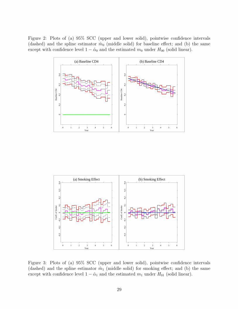
Figure 2: Plots of (a) 95% SCC (upper and lower solid), pointwise confidence intervals(dashed) and the spline estimator m0 (middle solid) for baseline effect; and (b) the sameexcept with confidence level 1− α0 and the estimated m0 under H00 (solid linear).

(a) Baseline CD4

0 1 2 3 4 5 6Year

00.

10.

20.

30.

4

Bas

elin

e C

D4

(b) Baseline CD4

0 1 2 3 4 5 6Year

00.

10.

20.

30.

4

Bas

elin

e C

D4

(a) Smoking Effect

0 1 2 3 4 5 6Year

-0.3

-0.2

-0.1

00.

10.

20.

30.

4

Coe

ff. o

f S

mok

e

(b) Smoking Effect

0 1 2 3 4 5 6Year

-0.3

-0.2

-0.1

00.

10.

20.

30.

4

Coe

ff. o

f S

mok

e

Figure 3: Plots of (a) 95% SCC (upper and lower solid), pointwise confidence intervals(dashed) and the spline estimator m1 (middle solid) for smoking effect; and (b) the sameexcept with confidence level 1− α1 and the estimated m1 under H01 (solid linear).

29

Figure 4: Plots of (a) 95% SCC (upper and lower solid), pointwise confidence intervals(dashed) and the spline estimator m2 (middle solid) for pre-infection CD4 effect; and (b) thesame except with confidence level 1− α2 and the estimated m2 under H02 (solid linear).

(a) PreCD4 Effect

0 1 2 3 4 5 6Year

-0.0

2-0

.01

00.

010.

020.

03

Coe

ff. o

f P

reC

D4

(b) PreCD4 Effect

0 1 2 3 4 5 6Year

-0.0

2-0

.01

00.

010.

020.

03

Coe

ff. o

f P

reC

D4

(a) Age Effect

0 1 2 3 4 5 6Year

-0.0

2-0

.01

00.

010.

020.

03

Coe

ff. o

f A

ge

(b) Age Effect

0 1 2 3 4 5 6Year

-0.0

2-0

.01

00.

010.

020.

03

Coe

ff. o

f A

ge

Figure 5: Plots of (a)95% SCC (upper and lower solid), pointwise confidence intervals(dashed) and the spline estimator m3 (middle solid) for age effect; and (b) the same ex-cept with confidence level 1− α3 and the estimated m3 under H03 (solid linear).

30

Table 1: Coverage percentages of the SCCs for functions m1 (left) and m2 (right), based on500 replications.

σ n 1− α c = 0.3 c = 0.5 c = 0.8 c = 1

1.0

2000.950 0.950, 0.952 0.944, 0.948 0.920, 0.904 0.886, 0.8840.990 0.990, 0.998 0.990, 0.990 0.976, 0.984 0.968, 0.974

4000.950 0.944, 0.948 0.950, 0.930 0.922, 0.912 0.908, 0.9040.990 0.996, 0.984 0.990, 0.988 0.984, 0.988 0.974, 0.966

6000.950 0.934, 0.962 0.954, 0.946 0.930, 0.952 0.930, 0.9240.990 0.992, 0.996 0.992, 0.986 0.988, 0.990 0.984, 0.990

8000.950 0.936, 0.934 0.960, 0.966 0.950, 0.964 0.956, 0.9340.990 0.998, 0.996 0.994, 0.994 0.986, 0.992 0.988, 0.988

0.5

2000.950 0.936, 0.948 0.952, 0.942 0.916, 0.900 0.912, 0.8900.990 0.988, 0.994 0.992, 0.990 0.972, 0.974 0.972, 0.972

4000.950 0.916, 0.930 0.936, 0.932 0.928, 0.916 0.904, 0.8980.990 0.994, 0.984 0.992, 0.988 0.996, 0.988 0.978, 0.976

6000.950 0.924, 0.948 0.952, 0.954 0.926, 0.958 0.936, 0.9380.990 0.996, 0.994 0.994, 0.986 0.984, 0.990 0.990, 0.994

8000.950 0.942, 0.900 0.950, 0.960 0.942, 0.962 0.960, 0.9380.990 0.996, 0.998 0.996, 0.994 0.990, 0.996 0.992, 0.988

31

Supplement to “A Simultaneous Confidence Corridor

for Varying Coefficient Regression with Sparse

Functional Data”

1Lijie Gu, 3Li Wang, 4,5Wolfgang K. Hardle and 1,2Lijian Yang

1Soochow University, 2Michigan State University, 3University of Georgia

4Humboldt-Universitat zu Berlin, 5Singapore Management University

In this document, we have collected a number of technical lemmas and their proofs. The

technical lemmas are used in the proofs of Propositions 1–4 in the paper.

Lemma B.1. (Bosq (1998), Theorem 1.2). Suppose that ξini=1 are i.i.d with E(ξ1) =

0, σ2 = E ξ21, and there exists c > 0 such that for r = 3, 4, . . ., E |ξ1|r ≤ cr−2r!E ξ21 < +∞.

Then for each n > 1, t > 0, P (|Sn| ≥√nσt) ≤ 2 exp

(−t2 (4 + 2ct/

√nσ)

−1), in which

Sn =∑n

i=1 ξi.

Lemma B.2. Under Assumptions (A2)–(A6), we have

An,1 = sup0≤J≤Ns,1≤l,l′≤d

∣∣∣⟨BJXl, BJXl′⟩NT− ⟨BJXl, BJXl′⟩

∣∣∣√⟨BJXl, BJXl⟩

√⟨BJXl′ , BJXl′⟩

= Op

√ log (n)

nhs

,

where for any J = 0, . . . , Ns and l, l′ = 1, . . . , d,

⟨BJXl, BJXl′⟩NT= N−1

T

∑n

i=1

∑Ni

j=1B2

J(Tij)XilXil′ ,

⟨BJXl, BJXl′⟩ = EB2

J(Tij)XilXil′= Hll′ .

1

Proof. Let ωi,J = ωi,J,l,l′ =∑Ni

j=1B2J(Tij)XilXil′ , then Eωi,J = EN1Hll′ ∼ 1 and

E (ωij,J)2 = E

∑Ni

j=1B2J(Tij)

2

E (XilXil′)2 ∼ h−1

s . Next define a sequence Dn = nα with

α(4 + η/2) > 1 and√

log (n)Dnn−1/2h

−1/2s → 0, n1/2h

1/2s D

−(3+η/2)n → 0, which necessitates

η > 2 according to Assumption (A5). We make use of the following truncated and tail

decomposition

Xill′ = XilXil′ = XDn

ill′,1 +XDn

ill′,2,

where XDn

ill′,1 = XilXil′I |XilXil′| > Dn, XDn

ill′,2 = XilXil′I |XilXil′| ≤ Dn. Define corre-

spondingly the truncated and tail parts of ωi,J as ωi,J,m = B2J(Tij)X

Dn

ill′,m,m = 1, 2. According

to Assumption (A5), for any l, l′ = 1, . . . , d,∞∑n=1

P |XnlXnl′| > Dn ≤∞∑n=1

E |XnlXnl′|4+η/2

D4+η/2n

≤ Cη

∞∑n=1

D−(4+η/2)n <∞.

By Borel-Cantelli Lemma, one has∑Ni

j=1B2J(Tij)X

Dn

ill′,1 = 0, a.s.. So we obtain

supJ,l,l′

∣∣∣∣∣n−1

n∑i=1

ωi,J,1

∣∣∣∣∣ = Oa.s.

(n−k), k ≥ 1,

and

Eωi,J,1 = E(XDn

ill′,1

)E

Ni∑j=1

B2J(Tij)

≤ D−(3+η/2)

n E |XilXil′|4+η/2 EN1 EB2J(Tij) ≤ cD−(3+η/2)

n .

Next we considerate the truncated part ωi,J,2. For large n, E (ωi,J,2) = E (ωi,J)−E (ωi,J,1) ∼ 1,

E (ωi,J,2)2 = E (ωi,J)

2 − E (ωi,J,1)2 ∼ h−1

s . Define ω∗i,J,2 = ωi,J,2 − E (ωi,J,2), then Eω∗

i,J,2 = 0,

and

E(ω∗i,J,2

)2= E (ωi,J,2)

2 − (Eωi,J,2)2 = E

Ni∑j=1

B2J(Tij)X

Dn

ill′,2

2

− U (1)

= E(XDn

ill′,2

)2E

Ni∑j=1

B2J(Tij)

2

− U (1) .

Note that

E(XDn

ill′,2

)2E

Ni∑j=1

B2J(Tij)

2

≥E (Xill′)

2 − E(XDn

ill′,1

)2E

Ni∑j=1

B4J(Tij)

≥

E (Xill′)

2 − U (1)EN1 EB

4J(Tij).

2

Thus, there exists cω such that for large n, E(ω∗i,J,2

)2 ≥ cω E (Xill′)2 h−1

s . Next for any r > 2

E∣∣ω∗

i,J,2

∣∣r = E |ωi,J,2 − E (ωi,J,2)|r ≤ 2r−1 (E |ωi,J,2|r + |E (ωi,J,2)|r)

= 2r−1

E∣∣XDn

ill′,2

∣∣r E ∣∣∣∣∣Ni∑j=1

B2J(Tij)

∣∣∣∣∣r

+ U(1)

= 2r−1

E ∣∣XDn

ill′,2

∣∣r E

r1+···+rNi=r∑

0≤r1,··· ,rNi≤r

(r

r1 · · · rNi

) Ni∏j=1

EB2rjJ (Tij)

+ U(1)

,then there exists Cω > 0 such that for any r > 2 and large n,

E∣∣ω∗

i,J,2

∣∣r ≤ 2r−1

[Dr−2

n E (Xill′)2 E

N r

1 max

Ni∏j=1

EB2rjJ (Tij)

+ U(1)

]≤ 2r−1

[Dr−2

n E (Xill′)2 (EN r

1 )CBh1−rs + U(1)

]≤ 2rDr−2

n (crNr!)1/2CBh

2−rs c−1

ω E(ω∗i,J,2

)2≤

(CωDnh

−1s

)r−2r!E

(ω∗i,J,2

)2,

which implies thatω∗i,J,2

ni=1

satisfies Cramer’s condition. Applying Lemma B.1 to∑n

i=1 ω∗i,J,2,

for r > 2 and any large enough δ > 0, P∣∣n−1

∑ni=1 ω

∗i,J,2

∣∣ ≥ δ (nhs)−1/2 (log(n))1/2

is

bounded by

2 exp

−δ2 (log(n))

4 + 2CωDnh−1s δ (log(n))1/2 n−1/2h

1/2s

≤ 2n−8.

Hence∞∑n=1

P

sup

0≤J≤Ns,1≤l,l′≤d

∣∣∣∣∣n−1

n∑i=1

ω∗i,J,2

∣∣∣∣∣ ≥ δ (nhs)−1/2 (log(n))1/2

<∞.

Thus, supJ,l,l′

∣∣n−1∑n

i=1 ω∗i,J,2

∣∣ = Oa.s.

(nhs)

−1/2 (log(n))1/2

as n → ∞ by Borel-Cantelli

Lemma. Furthermore,

supJ,l,l′

∣∣∣∣∣n−1

n∑i=1

ωi,J − Eωi,J

∣∣∣∣∣≤ sup

J,l,l′

∣∣∣∣∣n−1

n∑i=1

ωi,J,1

∣∣∣∣∣+ supJ,l,l′

∣∣∣∣∣n−1

n∑i=1

ω∗i,J,2

∣∣∣∣∣+ supJ,l,l′

|Eωi,J,1|

= Ua.s.

(n−k)+Oa.s.

(nhs)

−1/2 (log(n))1/2+ U

(D−(3+η/2)

n

)= Oa.s.

(nhs)

−1/2 (log(n))1/2.

3

Finally, we notice that

supJ,l,l′

∣∣∣⟨BJXl, BJXl′⟩NT− ⟨BJXl, BJXl′⟩

∣∣∣ = supJ,l,l′

∣∣∣∣∣(nN−1T

)n−1

n∑i=1

ωi,J − (EN1)−1 Eωi,J

∣∣∣∣∣≤ sup

J,l,l′(EN1)

−1∣∣(nEN1)N

−1T − 1

∣∣ ∣∣∣∣∣n−1

n∑i=1

ωi,J

∣∣∣∣∣+ supJ,l,l′

(EN1)−1

∣∣∣∣∣n−1

n∑i=1

ωi,J − Eωi,J

∣∣∣∣∣= Op

(n−1/2

)+Oa.s.

(nhs)

−1/2 (log(n))1/2= Op

(nhs)

−1/2 (log(n))1/2,

and ⟨BJXl, BJXl⟩ = Hll = U(1). Hence, An,1 = Op

(nhs)

−1/2 (log(n))1/2.

For the random matrix VJ defined in (18), the lemma below shows that its inverse can

be approximated by the inverse of a deterministic matrix H = E(XXT).

Lemma B.3. Under Assumptions (A2) and (A4)–(A6), for any J = 0, . . . , Ns, we have

V−1J = H−1 +Op

(nhs)

−1/2 (log(n))1/2. (B.1)

Proof. By Lemma B.2, we have∥∥∥VJ −H∥∥∥∞

= Op

(nhs)

−1/2 (log(n))1/2.

Using the fact that for any matrices A and B,

(A+ hB)−1 = A−1 − hA−1BA−1 +O(h2),

we obtain (B.1).

The next lemma implies that the difference between ξ (t) and ξ (t) and the difference

between ε(t) and ε(t) are both negligible uniformly over t ∈ [0, 1].

Lemma B.4. Under Assumption (A2)-(A6), for ξ(t), ε(t) given in (A.2), (A.3) and ξ(t),

ε(t) given in (A.4), (A.5), as n→ ∞, we have

supt∈[0,1]

∥∥∥ξ (t)− ξ (t)∥∥∥∞

= Op

n−1h−3/2

s log(n), (B.2)

supt∈[0,1]

∥ε (t)− ε (t)∥∞ = Op

n−1h−3/2

s log(n). (B.3)

4

Proof. Comparing the equations of ξ(t) and ξ(t) given in (A.2) and (A.4), we let

1

NT

n∑i=1

Ni∑j=1

BJ(Tij)Xil

d∑l′′=1

∞∑k=1

ξik,l′′ϕk,l′′ (Tij)Xil′′ =n

NT

d∑l′′=1

n∑i=1

Ωi,J,l′′,l.

where Ωi,J,l′′,l = Ωi = n−1[XilXil′′

∑∞k=1

∑Ni

j=1BJ(Tij)ϕk,l′′ (Tij)ξik,l′′

]. Note that EΩi = 0

and

σ2Ωi,n

= E(Ω2

i

∣∣∣(Tij, Ni, Xil)n,Ni,di=1,j=1,l=1

)= n−2

XilXil′′

∞∑k=1

Ni∑j=1

BJ(Tij)ϕk,l′′ (Tij)

2

≤ n−2

X2

ilX2il′′

∞∑k=1

Ni

Ni∑j=1

B2J(Tij)ϕ

2k,l′′ (Tij)

= n−2

X2

ilX2il′′Ni

Ni∑j=1

B2J(Tij)Gl′′ (Tij, Tij)

≤ Cn−2h−1

s X2ilX

2il′′N

2i .

Given (Tij, Ni, Xil)n,Ni,di=1,j=1,l=1,

σ−1Ωi,n

Ωi

ni=1

are i.i.d N (0, 1). It is easy to show that for

any large enough δ > 0,

P

|∑n

i=1Ωi|√∑ni=1 σ

2Ωi,n

≥ δ√

log(n)∣∣∣ (Tij, Ni, Xil)

n,Ni,di=1,j=1,l=1

≤ 2 exp

−1

2δ2 log(n)

≤ 2n−8,

P

∣∣∣∣∣n∑

i=1

Ωi

∣∣∣∣∣ ≥ δ

C log(n)

nhsn−1

n∑i=1

X2ilX

2il′′N

2i

1/2∣∣∣∣∣∣ (Tij, Ni, Xil)

n,Ni,di=1,j=1,l=1

≤ 2n−8.

Note that n−1∑n

i=1X2ilX

2il′′N

2i = Op (1), hence

∞∑n=1

P

sup

0≤J≤Ns,1≤l,l′′≤d

∣∣∣∣∣n∑

i=1

Ωi,J,l′′,l

∣∣∣∣∣ ≥ δ (nhs)−1/2 (log(n))1/2

<∞.

Thus, supJ,l,l′′ |∑n

i=1Ωi,J,l′′,l| = Op

(nhs)

−1/2 (log(n))1/2as n→ ∞ by Borel-Cantelli Lem-

ma. Furthermore, supJ,l

∣∣∣nN−1T

∑dl′′=1

∑ni=1Ωi,J,l′′,l

∣∣∣= Op

(nhs)

−1/2 (log(n))1/2. Finally,

according to Lemma B.1, we obtain (B.2). (B.3) is proved similarly.

5

Denote the inverse matrix of H by H−1 = zll′dl,l′=1. For any l = 1, . . . , d, we rewrite the

l-th element of ξl(t) and εl(t) in (A.4) and (A.5) as the following

ξl(t) = c−1/2J(t),nN

−1T

d∑l′′=1

n∑i=1

∞∑k=1

Rik,ξ,J(t),l′′,lξik,l′′ , (B.4)

εl(t) = c−1/2J(t),nN

−1T

n∑i=1

N∑j=1

Rij,ε,J(t),lεij, (B.5)

where for any 0 ≤ J ≤ Ns,

Rik,ξ,J,l′′,l =

(d∑

l′=1

zll′Xil′Xil′′

)Ni∑j=1

BJ (Tij)ϕk,l′′ (Tij)

, (B.6)

Rij,ε,J,l =

(d∑

l′=1

zll′Xil′

)BJ (Tij) σ (Tij) . (B.7)

Further denote

Sill′′ =

(d∑

l′=1


)2

, sll′′ = E (Sill′′) , 1 ≤ l, l′′ ≤ d. (B.8)

Lemma B.5. Under Assumptions (A2)-(A6), for Rik,ξ,J,l′′,l, Rij,ε,J,l in (B.6), (B.7),

E

(∞∑k=1

R2ik,ξ,J,l′′,l

)= c−1

J,nsll′′

[(EN1)

∫bJ (u)Gl′′ (u, u) f (u) du

+E N1(N1 − 1)∫bJ (u) bJ (v)Gl′′ (u, v) f (u) f (v) dudv

],

ER2ij,ε,J,l = c−1

J,nzll

∫bJ (u)σ

2 (u) f (u) du,

for 0 ≤ J ≤ Ns and 0 ≤ l, l′′ ≤ d. In addition, there exist 0 < cR < CR <∞, such that

cRsll′′ ≤ E

(∞∑k=1

R2ik,ξ,J,l′′,l

)≤ CRsll′′ , cR ≤ ER2

ij,ε,J,l ≤ CR,

for 0 ≤ J ≤ Ns, 0 ≤ l, l′′ ≤ d, and as n→ ∞

An,ξ = supJ,l′′,l

∣∣∣∣∣n−1

n∑i=1

∞∑k=1

R2ik,ξ,J,l′′,l − E

(∞∑k=1

R2ik,ξ,J,l′′,l

)∣∣∣∣∣ = Oa.s.

(nhs)

−1/2 (log(n))1/2,

An,ε = supJ,l

∣∣∣∣∣N−1T

n∑i=1

Ni∑j=1

R2ij,ε,J,l − ER2

ij,ε,J,l

∣∣∣∣∣ = Oa.s.

(nhs)

−1/2 (log(n))1/2.

6

Proof. By independence of Tij∞j=1, Xildl=1 , Ni, the definition of BJ and (B.8),

E

(∞∑k=1

R2ik,ξ,J,l′′,l

)= E (Sill′′)E

∞∑k=1

Ni∑j=1

BJ (Tij)ϕk,l′′ (Tij)

2

= sll′′ E

Ni∑j=1

Ni∑j′=1

BJ (Tij)BJ (Tij′)Gl′′ (Tij, Tij′)

= sll′′c−1J,n

(EN1)

∫bJ (u)Gl′′ (u, u) f (u) du

+E N1(N1 − 1)∫bJ (u) bJ (v)Gl′′ (u, v) f (u) f (v) dudv

,

thus there exist constants 0 < cR < CR <∞ such that cRsll′′ ≤ E(∑∞

k=1R21k,ξ,J,l′′,l

)≤ CRsll′′ ,

0 ≤ J ≤ Ns, 0 ≤ l, l′′ ≤ d.

If sll′′ = 0, one has Sill′′ = 0, almost surely. Hence n−1∑n

i=1

∑∞k=1R

2ik,ξ,J,l′′,l = 0, almost

surely. In the case of sll′′ > 0, let ζ i,J = ζ i,J,l′′,l =∑∞

k=1R2ik,ξ,J,l′′,l for brevity. Under

Assumption (A5), it is easy to verify that

0 < s2ll′′ ≤ E (Sill′′)2 ≤ d3

d∑l′=1

E |zll′Xil′Xil′′ |4 ≤ d3d∑

l′=1

zll′E |Xil′|8 E |Xil′′ |8

1/2<∞.

So for large n,

E(ζ i,J)2

= E

(Sill′′)2

(Ni∑j=1

Ni∑j′=1


)2

≥ E (Sill′′)2 1

4c2G,l′′ E

Ni∑j=1

BJ (Tij)

4

≥ cE

Ni∑j=1

B4J (Tij) ≥ ch−1

s ,

and

E(ζ i,J)2 ≤ E (Sill′′)

2 4C2G,l′′ E

Ni∑j=1

BJ (Tij)

4

≤ cE

[N3

1

Ni∑j=1

EB4J (Tij)

∣∣∣∣∣N1

]≤ cEN4

1 EB4J (Tij) ≤ ch−1

s .

Define a sequence Dn = nα that satisfies α (2 + η/4) > 1, Dnn−1/2h

−1/2s (log(n))1/2 → 0,

n1/2h1/2s D

−(1+η/4)n → 0, which requires η > 4 provided by Assumption (A5). We make use of

7

the following truncated and tail decomposition

Sill′′ =d∑

l′=1

d∑l′′′=1

zll′zll′′′Xil′Xil′′′X2il′′ = SDn

ill′′,1 + SDn

ill′′,2,

where

SDn

ill′′,1 =d∑

l′=1

d∑l′′′=1

zll′zll′′′Xil′Xil′′′X2il′′I

∣∣Xil′Xil′′′X2il′′

∣∣ > Dn

,

SDn

ill′′,2 =d∑

l′=1

d∑l′′′=1



∣∣ ≤ Dn

.

Define correspondingly the truncated and tail parts of ζ i,J as

ζ i,J,m = SDn

ill′′,m

Ni∑j=1

Ni∑j′=1

BJ (Tij)BJ (Tij′)Gl′′ (Tij, Tij′) , m = 1, 2.

According to Assumption (A5), for any l′, l′′, l′′′ = 1, . . . , d,

∞∑n=1

P∣∣Xnl′Xnl′′′X

2nl′′

∣∣ > Dn

≤

∞∑n=1

E |Xnl′Xnl′′′X2nl′′ |

2+η/4

D2+η/4n

≤ Cη

∞∑n=1

D−(2+η/4)n <∞.

Borel-Cantelli Lemma implies that

Pω∣∣∃N (ω) ,

∣∣Xnl′Xnl′′′X2nl′′ (ω)

∣∣ ≤ Dn for n > N (ω)= 1,

Pω∣∣∃N (ω) ,

∣∣Xil′Xil′′′X2il′′ (ω)

∣∣ ≤ Dn, i = 1, . . . , n for n > N (ω)= 1,

Pω∣∣∃N (ω) , I

∣∣Xil′Xil′′′X2il′′ (ω)

∣∣ > Dn

= 0, i = 1, . . . , n for n > N (ω)

= 1.

Furthermore, one has

n−1

n∑i=1

SDn

ill′′,1

Ni∑j=1

Ni∑j′=1


= 0, a.s.

Therefore, one has

supJ,l,l′′

∣∣∣∣∣n−1

n∑i=1

ζ i,J,1

∣∣∣∣∣ = Oa.s.

(n−k), k ≥ 1.

Notice that

E(SDn

ill′′,1

)= E

[d∑

l′=1

d∑l′′′=1



∣∣ > Dn

]

≤ D−(1+η/4)n

d∑l′=1

d∑l′′′=1

zll′zll′′′ E∣∣Xil′Xil′′′X

2il′′

∣∣2+η/4

≤ cD−(1+η/4)n .

8

So for large n,

E(ζ i,J,1

)= E

(SDn

ill′′,1

)E

Ni∑j=1

Ni∑j′=1


≤ cD−(1+η/4)n 2CG,l′′ E

Ni∑j=1

BJ (Tij)

2

≤ cD−(1+η/4)n E

(N2

1

)EB2

J (Tij)

≤ cD−(1+η/4)n .

Next we considerate the truncated part ζ i,J,2. For large n, E(ζ i,J,2

)= E

(ζ i,J)−E

(ζ i,J,1

)∼ 1,

E(ζ i,J,2

)2= E

(ζ i,J)2 − E

(ζ i,J,1

)2 ∼ h−1s . Define ζ∗i,J,2 = ζ i,J,2 − E

(ζ i,J,2

), then E ζ∗i,J,2 = 0,

and there exist cζ , Cζ > 0 such that for r > 2 and large n,

E(ζ∗i,J,2

)2= E

∣∣SDn

ill′′,2

∣∣2 E ∣∣∣∣∣Ni∑j=1

Ni∑j′=1


∣∣∣∣∣2

−(E ζ i,J,2

)2≥

E |Sill′′ |2 − E

∣∣SDn

ill′′,1

∣∣2 1

4c2G,l′′ E

Ni∑j=1

BJ (Tij)

4

− U(1)

≥E |Sill′′|2 − U(1)

1

4c2G,l′′ E

Ni∑j=1

B4J (Tij)

− U(1)

≥ 1

2E |Sill′′ |2

1

4c2G,l′′ EN1 EB

4J (Tij)− U(1)

≥ cζ E |Sill′′ |2 h−1s ,

and

E∣∣ζ∗i,J,2∣∣r = E

∣∣ζ i,J,2 − E(ζ i,J,2

)∣∣r ≤ 2r−1(E∣∣ζ i,J,2∣∣r + ∣∣E (ζ i,J,2)∣∣r)

= 2r−1

E∣∣SDn

ill′′,2

∣∣r E ∣∣∣∣∣Ni∑j=1

Ni∑j′=1


∣∣∣∣∣r

+ U(1)

≤ 2r−1

(cDn)r−2 E |Sill′′ |2 (2CG,l′′)

r E

Ni∑j=1

BJ(Tij)

2r

+ U(1)

≤ 2r−1

[(cDn)

r−2 E |Sill′′ |2 (2CG,l′′)r (EN2r

1

)CBh

1−rs + U(1)

]≤ 2r (cDn)

r−2 (2CG,l′′)r crNr!CBh

2−rs c−1

ζ E(ζ∗i,J,2

)2≤

(CζDnh

−1s

)r−2r!E

(ζ∗i,J,2

)2,

9

which implies thatζ∗i,J,2

ni=1

satisfies Cramer’s condition. Applying Lemma B.1 to∑n

i=1 ζ∗i,J,2,

for r > 2 and any large enough δ > 0,

P

∣∣∣∣∣n−1

n∑i=1

ζ∗i,J,2

∣∣∣∣∣ ≥ δ(nhs)−1/2(log(n))1/2

≤ 2 exp

−δ2 log(n)

4 + 2CζDnh−1s δ (log(n))1/2 n−1/2h

1/2s

≤ 2n−8.

Hence∞∑n=1

P

supJ,l′′,l

∣∣∣∣∣n−1

n∑i=1

ζ∗i,J,2

∣∣∣∣∣ ≥ δ (nhs)−1/2 (log(n))1/2

<∞.

Thus, supJ,l′′,l

∣∣n−1∑n

i=1 ζ∗i,J,2

∣∣ = Oa.s.

(nhs)

−1/2 (log(n))1/2

as n → ∞ by the Borel-

Cantelli lemma. Furthermore, we have

An,ξ ≤ supJ,l,l′′

∣∣∣∣∣n−1

n∑i=1

ζ i,J,1

∣∣∣∣∣+ supJ,l′′,l

∣∣∣∣∣n−1

n∑i=1

ζ∗i,J,2

∣∣∣∣∣+ supJ,l′′,l

∣∣E (ζ i,J,1)∣∣= Ua.s.

(n−k)+Oa.s.

(nhs)

−1/2 (log(n))1/2+ U

(D−(1+η/4)

n

)= Oa.s.

(nhs)

−1/2 (log(n))1/2.

The properties of Rij,ε,J,l are obtained similarly.

Next define two d× d matrices

Γξ,n(t) = c−1J(t),nN

−2T

d∑l′′=1

n∑i=1

∞∑k=1

Ni∑j=1

BJ(t)(Tij)ϕk,l′′ (Tij)

2

X2il′′XiX

Ti ,

Γε,n(t) = c−1J(t),nN

−2T

n∑i=1

Ni∑j=1

B2J(t)(Tij)σ

2 (Tij)XiXTi .

Lemma B.6. For any t ∈ R, the conditional covariance matrices of ξ (t) and ε (t) on

(Tij, Ni, Xil)n,Ni,di=1,j=1,l=1 are

Σξ,n(t) = Eξ (t) ξ

T(t)∣∣∣(Tij, Ni, Xil)

n,Ni,di=1,j=1,l=1

= H−1Γξ,n(t)H

−1,

Σε,n(t) = Eε (t) εT (t)


= H−1Γε,n(t)H

−1,

and with Σn(t) defined in (7),

supt∈[0,1]

∥Σξ,n(t) +Σε,n(t) −Σn(t)∥∞ = Oa.s.

n−3/2h−3/2

s (log(n))1/2. (B.9)

10

Proof. Note that

ξ (t) ξT(t) = c−1

J(t),nH−1

1

N2T

n∑i=1

Ni∑j=1

BJ(t)(Tij)Xil

d∑l′′=1

∞∑k=1


×n∑

i=1

Ni∑j=1

BJ(t)(Tij)Xil′

d∑l′′=1

∞∑k=1


d

l,l′=1

H−1.

Thus,

Σξ,n(t) = Eξ (t) ξ

T(t)∣∣∣(Tij, Ni, Xil)

n,Ni,di=1,j=1,l=1

= c−1

J(t),nH−1

×

N−2T

d∑l′′=1

n∑i=1

∞∑k=1

Ni∑j=1

BJ(t)(Tij)ϕk,l′′ (Tij)

2

X2il′′XiX

Ti

H−1

= H−1Γξ,n(t)H−1.

Similarly, we can derive the conditional covariance matrix of ε (t). Next let

Ψik,ξ,J,l,l′,l′′ =

Ni∑j=1

BJ(Tij)ϕk,l′′ (Tij)

2

X2il′′XilXil′ ,

Ψij,ε,J,l,l′ = B2J(Tij)σ

2 (Tij)XilXil′ .

Similar to the proof of Lemma B.5,

E

(∞∑k=1

Ψik,ξ,J,l,l′,l′′

)= c−1

J,n E(X2

il′′XilXil′) [

(EN1)

∫χJ

Gl′′ (u, u) f (u) du+

+E N1(N1 − 1)∫χJ×χJ

Gl′′ (u, v) f (u) f (v) dudv

],

EΨij,ε,J,l,l′ = c−1J,n E (XilXil′)

∫χJ

σ2 (u) f (u) du,

and as n→ ∞,

supJ,l,l′,l′′

∣∣∣∣∣n−1

n∑i=1

∞∑k=1

Ψik,ξ,J,l,l′,l′′ − E

(∞∑k=1


)∣∣∣∣∣ = Oa.s.

(nhs)

−1/2 (log(n))1/2,

supJ,l,l′

∣∣∣∣∣N−1T

n∑i=1

Ni∑j=1

Ψij,ε,J,l,l′ − EΨij,ε,J,l,l′

∣∣∣∣∣ = Oa.s.

(nhs)

−1/2 (log(n))1/2.

11

Furthermore,

supJ,l,l′,l′′

∣∣∣∣∣N−2T

n∑i=1

∞∑k=1

Ψik,ξ,J,l,l′,l′′ − n−1 (EN1)−2 E

(∞∑k=1


)∣∣∣∣∣≤ sup

J,l,l′,l′′n−1 (EN1)

−2

∣∣∣∣∣(nEN1

NT

)2

− 1

∣∣∣∣∣∣∣∣∣∣n−1

n∑i=1

∞∑k=1


∣∣∣∣∣+

∣∣∣∣∣n−1

n∑i=1

∞∑k=1

Ψik,ξ,J,l,l′,l′′ − E

(∞∑k=1


)∣∣∣∣∣

= Oa.s.

n−3/2h−1/2

s (log(n))1/2,

and

supJ,l,l′

∣∣∣∣∣N−2T

n∑i=1

Ni∑j=1

Ψik,ε,J,l,l′ − (nEN1)−1 EΨik,ε,J,l,l′

∣∣∣∣∣≤ sup

J,l,l′(nEN1)

−1

∣∣∣∣nEN1

NT

− 1

∣∣∣∣∣∣∣∣∣N−1

T

n∑i=1

Ni∑j=1

Ψik,ε,J,l,l′

∣∣∣∣∣+

∣∣∣∣∣N−1T

n∑i=1

Ni∑j=1

Ψik,ε,J,l,l′ − EΨik,ε,J,l,l′

∣∣∣∣∣

= Oa.s.

n−3/2h−1/2

s (log(n))1/2.

Notice that

Σn(t) = H−1c−1J(t),n (nEN1)

−1

(EN1)

−1 E

(d∑

l′′=1

∞∑k=1

Ψik,ξ,J(t),l,l′,l′′

)+ EΨij,ε,J(t),l,l′

d

l,l′=1

×H−1,

Σξ,n(t) +Σε,n(t)

= H−1c−1J(t),nN

−2T

d∑

l′′=1

n∑i=1

∞∑k=1

Ψik,ξ,J(t),l,l′,l′′ +n∑

i=1

Ni∑j=1

Ψij,ε,J(t),l,l′

d

l,l′=1

H−1,

and (A.1) implies supt∈[0,1]∣∣cJ(t),n∣∣ = O (hs). Hence (B.9) holds.

Given (Tij, Ni, Xil)n,Ni,di=1,j=1,l=1, let σ

2ξl,n

(t) and σ2εl,n

(t) be the conditional variances of ξl(t)

and εl(t) defined in (A.4) and (A.5), respectively. Lemma B.6 implies that

supt∈[0,1]

∣∣∣σ2ξl,n

(t) + σ2εl,n

(t)− σ2n,ll(t)

∣∣∣ = Oa.s.

n−3/2h−3/2

s (log(n))1/2. (B.10)

12

Lemma B.7. Under Assumptions (A2)-(A6), for l = 1, . . . , d, ηl(t) defined in (A.6) is

a Gaussian process consisting of (Ns + 1) standard normal variablesηJ,lNs

J=0such that

ηl(t) = ηJ(t),l for t ∈ [0, 1], and there exists a constant C > 0 such that for large n,

sup0≤J =J ′≤Ns


∣∣ ≤ Chs.

Proof. For any fixed l = 1, . . . , d and 0 ≤ J ≤ Ns, LηJ,l


=

N (0, 1) by Assumption (A2), so LηJ,l= N (0, 1), for 0 ≤ J ≤ Ns.

Next we derive the upper bound for sup0≤J =J ′≤Ns


∣∣. LetRξ,J(t),l = N−1

T

d∑l′′=1

n∑i=1

∞∑k=1

R2ik,ξ,J(t),l′′,l, Rε,J(t),l = N−1

T

n∑i=1

Ni∑j=1

R2ij,ε,J(t),l,

then we have

σξl,n(t) =

c−1J(t),nN

−2T

d∑l′′=1

n∑i=1

∞∑k=1

R2ik,ξ,J(t),l′′,l

1/2

=c−1J(t),nN

−1T Rξ,J(t),l

1/2

,

σεl,n(t) =

c−1J(t),nN

−2T

n∑i=1

Ni∑j=1

R2ij,ε,J(t),l

1/2

=c−1J(t),nN

−1T Rε,J(t),l

1/2

.

For J = J ′, by (B.7) and the definition of BJ ,

Rij,ε,J,lRij,ε,J ′,l =

(d∑

l′=1

zll′Xil′

)2

BJ (Tij)BJ ′ (Tij)σ2 (Tij) = 0,

along with the conditional independence of ξl(t), εl(t) on (Tij, Ni, Xil)n,Ni,di=1,j=1,l=1, and inde-

pendence of ξik,l, Tij, Ni, Xildl=1, 1 ≤ j ≤ Ni, 1 ≤ i ≤ n, k = 1, 2, . . .,

E(ηJ,lηJ ′,l

)= E

[(Rξ,J,l + Rε,J,l)

−1/2(Rξ,J ′,l + Rε,J ′,l)−1/2

×N−1T E

(d∑

l′′=1

n∑i=1

∞∑k=1

Rik,ξ,J,l′′,lξik,l′′

)(d∑

l′′=1

n∑i=1

∞∑k=1

Rik,ξ,J ′,l′′,lξik,l′′

)

+

(n∑

i=1

Ni∑j=1

Rij,ε,J,lεij

)(n∑

i=1

Ni∑j=1

Rij,ε,J ′,lεij

)∣∣∣∣∣ (Tij, Ni, Xil)n,Ni,di=1,j=1,l=1

]= ECn,J,J ′,l,

in which

Cn,J,J ′,l = (Rξ,J,l + Rε,J,l)−1/2(Rξ,J ′,l + Rε,J ′,l)

−1/2

N−1

T

d∑l′′=1

n∑i=1

∞∑k=1

Rik,ξ,J,l′′,lRik,ξ,J ′,l′′,l

.

13

Note that according to definitions of Rik,ξ,J,l′′,l, Rij,ε,J,l, and Lemma B.5, for 0 ≤ J ≤ Ns

Rξ,J(t),l + Rε,J(t),l ≥ Rε,J(t),l ≥ ER2ij,ε,J,l − An,ε ≥ cR − An,ε,

P

inf0≤J =J ′≤Ns

(Rξ,J,l + Rε,J,l)(Rξ,J ′,l + Rε,J ′,l)

≥

cR − δ

√log(n)

nhs

2 ≥ 1− 2n−8.

Thus for large n, with probability ≥ 1−2n−8, the denominator of Cn,J,J ′,l is uniformly greater

than c2R/4. On the other hand, we consider the numerator of Cn,J,J ′,l.

E

(N−1

T

d∑l′′=1

n∑i=1

∞∑k=1


)= E

N−1T

d∑l′′=1

n∑i=1

(d∑

l′=1


)2

×

(Ni∑j=1

Ni∑j′=1

BJ (Tij)BJ ′ (Tij′)Gl′′ (Tij, Tij′)

)∼ hs.

Applying Bernstein’s inequality, there exists C0 > 0 such that, for large n,

P

(sup

0≤J =J ′≤Ns

∣∣∣∣∣N−1T

d∑l′′=1

n∑i=1

∞∑k=1


∣∣∣∣∣ ≤ C0hs

)≥ 1− 2n−8.

Putting the above together, for large n, C1 = C0 (c2R/4)

−1,

P

(sup

0≤J =J ′≤Ns

|Cn,J,J ′,l| ≤ C1hs

)≥ 1− 4n−8.

Note that as a continuous random variable, sup0≤J =J ′≤Ns|Cn,J,J ′,l| ∈ [0, 1] , thus

E

(sup

0≤J =J ′≤Ns

|Cn,J,J ′,l|)

=

∫ 1

0

P

(sup

0≤J =J ′≤Ns

|Cn,J,J ′,l| > u

)du.

For large n, C1hs < 1 and then E(sup0≤J =J ′≤Ns,l |Cn,J,J ′|

)is∫ C1hs

0

P

sup

0≤J =J ′≤Ns,l|Cn,J,J ′,l| > u

du+

∫ 1

C1hs

P

sup

0≤J =J ′≤Ns,l|Cn,J,J ′,l| > u

du

≤∫ C1hs

0

1du+

∫ 1

C1hs

4n−8du ≤ C1hs + 4n−8 ≤ Chs

for some C > 0 and large enough n. The lemma now follows from

sup0≤J =J ′≤Ns

|E (Cn,J,J ′,l)| ≤ E

(sup

0≤J =J ′≤Ns

|Cn,J,J ′,l|)

≤ Chs.

This completes the proof of the lemma.

14

Lemma B.8. Under Assumptions (A2)-(A6), for ηl(t), σn,ll(t), l = 1, . . . , d, defined in (A.6)

and (7), one has∣∣∣σn,ll(t)

−1ξl(t) + εl(t)

− ηl(t)

∣∣∣ = |rn,l(t)− 1| |ηl(t)|, where rn,l(t) =

σ−1n,ll(t)

σ2ξl,n

(t) + σ2εl,n

(t)1/2

, and as n→ ∞,

supt∈[0,1]

aNs+1 |rn,l(t)− 1| = Oa.s.

(nhs)

−1/2 (log (Ns + 1) log(n))1/2.

Proof. By Lemma B.5, σ2n,ll(t) in (7) can be rewritten as

σ2n,ll(t) = c−1

J(t),n (nEN1)−1

(EN1)

−1d∑

l′′=1

E

(∞∑k=1

R2ik,ξ,J(t),l′′,l

)+ ER2

ij,ε,J(t),l

∼ n−1h−1

s .

Hence, according to (B.10) and (10),

supt∈[0,1]

aNs+1 |rn,l(t)− 1| = supt∈[0,1]

aNs+1

∣∣∣∣σ−1n,ll(t)

σ2ξl,n

(t) + σ2εl,n

(t)1/2

− 1

∣∣∣∣≤ sup

t∈[0,1]

aNs+1

∣∣∣σ−2n,ll(t)

σ2ξl,n

(t) + σ2εl,n

(t)− 1∣∣∣

= supt∈[0,1]

aNs+1σ

−2n,ll(t)

∣∣∣σ2ξl,n

(t) + σ2εl,n

(t)− σ2n,ll(t)

∣∣∣= Oa.s.

(nhs)

−1/2 (log (Ns + 1) log(n))1/2.

This completes the proof.

15

SFB 649 Discussion Paper Series 2014

For a complete list of Discussion Papers published by the SFB 649,

please visit http://sfb649.wiwi.hu-berlin.de.

001 "Principal Component Analysis in an Asymmetric Norm" by Ngoc Mai

Tran, Maria Osipenko and Wolfgang Karl Härdle, January 2014.

002 "A Simultaneous Confidence Corridor for Varying Coefficient Regression

with Sparse Functional Data" by Lijie Gu, Li Wang, Wolfgang Karl Härdle

and Lijian Yang, January 2014.

SFB 649, Spandauer Straße 1, D-10178 Berlin

http://sfb649.wiwi.hu-berlin.de

This research was supported by the Deutsche

Forschungsgemeinschaft through the SFB 649 "Economic Risk".

Documents

A Simultaneous Confidence Corridor for Varying - SFB 649