Embed Size (px)
Citation preview

A Simulation Estimator for Dynamic Models of Discrete Choice
V Joseph Hotz Robert A Miller Seth Sanders Jeffrey Smith
The Review of Economic Studies Vol 61 No 2 (Apr 1994) pp 265-289
Stable URL
httplinksjstororgsicisici=0034-65272819940429613A23C2653AASEFDM3E20CO3B2-9
The Review of Economic Studies is currently published by The Review of Economic Studies Ltd
Your use of the JSTOR archive indicates your acceptance of JSTORs Terms and Conditions of Use available athttpwwwjstororgabouttermshtml JSTORs Terms and Conditions of Use provides in part that unless you have obtainedprior permission you may not download an entire issue of a journal or multiple copies of articles and you may use content inthe JSTOR archive only for your personal non-commercial use
Please contact the publisher regarding any further use of this work Publisher contact information may be obtained athttpwwwjstororgjournalsreslhtml
Each copy of any part of a JSTOR transmission must contain the same copyright notice that appears on the screen or printedpage of such transmission
The JSTOR Archive is a trusted digital repository providing for long-term preservation and access to leading academicjournals and scholarly literature from around the world The Archive is supported by libraries scholarly societies publishersand foundations It is an initiative of JSTOR a not-for-profit organization with a mission to help the scholarly community takeadvantage of advances in technology For more information regarding JSTOR please contact supportjstororg
httpwwwjstororgTue Jul 24 085821 2007
Review of Economic Studies (1994) 61 265-289 0 1994 The Review of Economic Studies Limited
A Simulation Estimator for Dynamic Models of
Discrete Choice V JOSEPH HOTZ University of Chicago
ROBERT A MILLER Carnegie Mellon University
SETH SANDERS Carnegie Mellon University
and
JEFFREY SMITH University of Chicago
First version received February 1992 Jinal version accepted September 1993 (Eds)
This paper analyses a new estimator for the structural parameters of dynamic models of discrete choice Based on an inversion theorem due to Hotz and Miller (1993) which establishes the existence of a one-to-one mapping between the conditional valuation functions for the dynamic problem and their associated conditional choice probabilities we exploit simulation techniques to estimate models which do not possess terminal states In this way our Conditional Choice Simula- tion (CCS) estimator complements the Conditional Choice Probability (CCP) estimator of Hotz and Miller (1993) Drawing on work in empirical process theory by Pakes and Pollard (1989) we establish its large sample properties and then conduct a Monte Carlo study of Rusts (1987) model of bus engine replacement to compare its small sample properties with those of Maximum Likelihood (ML)
1 INTRODUCTION
Following Miller (1982 1984) and Wolpin (1984) there have been many applications of maximum likelihood (ML) estimation techniques to dynamic models of discrete choice (See the survey by Eckstein and Wolpin (1989)) There are several reasons for estimating econometric models that are explicitly derived from dynamic choice-theoretic frameworks over those which have less explicit connections to economic theory The fact that estimated parameters can be interpreted within an economic framework automatically provides a common language for economists to discuss the results (within and between empirical studies) Similarly an economic interpretation can be readily attached to hypothesis tests Finally predictions about economic phenomena can be made by conducting exercises in comparative dynamics on the economic models that support the estimation
Along with this growing literature there has developed an awareness of the very high computational costs of undertaking ML in such models which in turn has sparked
265
266 REVIEW OF ECONOMIC STUDIES
interest in alternative methods of estimation One of these is to replace the assumption that agents optimize with specifications of behaviour that yield computationally less bur- densome decisions rules for estimation purposes For example Hotz and Miller (1986 1988) restrict the space of feasible decision rules to index functions that are linear in the state variables Stock and Wise (1990) also attempt to simplify the calculation of decision rules in estimation by incorrectly passing an expectations operator through the (nonlinear) maximization operator Recently Hotz and Miller (1993) developed a new strategy for estimating dynamic models of discrete choices which avoids the high cost of recursively computing the valuation function many times a cost associated with ML estimation without compromising the rationality assumption Their method which we refer to as the conditional choice probability (CCP) estimator is based on an alternative representation of the valuation function This representation expresses the valuation function as a weighted sum of the possible utility streams that might occur Therein the weights are conditional probabilities of the choices prescribed by sequential optimization of future realizations of stochastic variables In addition the unobserved components of these utility streams are corrected for the dynamic selection which arises from optimizing behaviour expressing these corrections in terms of conditional choice probabilities Given consistent estimates of the conditional choice probabilities and the probabilities determining the other stochastic variables relatively straightforward estimators of the structural parameters can be formed
The CCP estimation procedure can be applied to a wide range of stochastic problems in discrete choice However to illustrate it Hotz and Miller (1993) focus on a model from a much more restrictive class The defining characteristic of this class called the terminal state property is the existence of at least one action at each decision node (called a terminating action) which if taken would eliminate the differential impact of subsequent choices on the state variables over the remainder of the agents horizon Within this class which includes optimal stopping problems the number of states for which conditional choice probabilities must be estimated is considerably reduced
In dynamic choice models which do not have the terminal state property calculation of valuation functions remains problematic even when using the alternative representation To characterize the utility of a current action the econometrician must assess the expected utility of subsequent choices where the latter are assumed to be made optimally The number of these future feasible actions can become large both in terms of the number feasible at a point in time and the number of periods remaining in an agents horizon In essence the decision tree associated with each current action tends to have many branches This increases the complexity of implementing the CCP estimator as the conditional choice probabilities must be estimated for all these nodes (or future feasible choices)
In this paper we consider how to estimate models lacking this terminal state property Rather than evaluating the expected utilities associated with all feasible future paths we show that one need only consider those associated with a path of simulated future choices These simulated paths are generated in a manner consistent with optimal decision-making by exploiting (estimates of) the future conditional choice probabilities and the transition probabilities governing outcomes Estimating equations for the structural parameters of a model can be formed using the utilities associated with the simulated paths to form valuation functions We call the resulting estimator the conditional choice simulation
1 For example structural models of optimal retirement or sterilization choice have this property 2 This lack of terminating actions also greatly increases the complexity of the maximum likelihood strateg-
ies as it entails integrating over all future paths
267 HOTZ et al DYNAMIC DISCRETE CHOICE
(CCS) estimator and show that this estimator is co consistent and asymptotically normal for a sample of size N
Like the CCP estimator the CCS estimator requires using only unrestricted estimates of the conditional choice and transition probabilities But in contrast to the CCP estima- tor the new estimator proposed here does not necessarily require estimation of probabili- ties for all feasible future choice and transitions Instead it requires the estimation only of those choice and transition probabilities associated with the nodes of some agents simulated future path While the usefulness of simulation in estimating structural models of sequential decision-making has been pointed out and exploited by others our approach differs from earlier work in that it avoids both the backwards recursion computation of valuation functions (by exploiting the representation developed in Hotz and Miller (1993)) and integration over all future paths (via simulation of a single future path)4 Finally our use of simulation methods in forming estimators is different from the applications presented in Pakes and Pollard (1989) and McFadden (1989) in that the simulated paths do not depend on the structural parameter estimates a feature which facilitates estimation in two ways First new simulated paths are not generated for each different set of structural parameter values being evaluated in the estimation algorithm Second for a given sample the criterion function for evaluating the structural parameters is typically a smooth func- tion so derivative-based optimization algorithms can be applied
Finally in contrast to ML both the CCP and CCS estimators separate the problem of estimating parameters which generated the data from the problem of solving the dynamic programming model for any given set of parameters This means that while the reduction in computer machine time is quite dramatic when either alternative to ML is used in estimation substantial amounts of computer programming time may be required to solve for the optimal decision rules when undertaking comparative dynamic exercises However as Hotz and Miller (1993) demonstrate this is not necessarily the case it depends on the specific nature of the exercise under consideration
The remainder of the paper is organized as follows The next section describes the class of dynamic discrete-choice models to be considered and reviews the formulation of valuation functions developed in Hotz and Miller (1993) In Section 3 we develop the CCS estimator and establish its asymptotic properties for finite-horizon models Section 4 extends these results to infinite-horizon Markov models Then in Section 5 we present a Monte Carlo study of the small sample performance of this estimator in the renewal model estimated in Rust (1987) Several variations on the CCS estimator are implemented and compared to the maximum likelihood estimator
2 THE MODEL AND REPRESENTING CONDITIONAL VALUATION FUNCTIONS
To maintain comparability with Hotz and Miller (1993) we restrict the analysis in this and the following section to finite-horizon discrete-choice models In each period
3 See Pakes and Pollard (1989) Berkovec and Stern (1991) and Altug and Miller (1991) 4 Our approach to estimation of dynamic models is quite similar to that used in Altug and Miller (1991)
The main features distinguishing our work from Altug and Miller (1991) are that they use simulation methods to deal with common shocks hitting the population and assume a form of finite history dependence to reduce the computational burden associated with CCP estimation This paper assumes that there are no aggregate shocks but does not impose the assumption of finite history dependence These differences affect the proof strategies used to establish the respective results because the criterion function which defines Altug and Millers (1991) estimator is smooth in the parameters while the criterion function for the CCS estimator is not continuous Note that the parameter space includes both the structural parameters 0and the incidental choice and transition probabilities y As mentioned in the text changing the estimates of the conditional choice probabilities (which occurs as the sample size increases) creates jumps in the simulated paths
268 REVIEW OF ECONOMIC STUDIES
t euro T = (1 T a typical agent chooses an action for which there are J alternatives Let
denote the agents decision about action j in period t where d= 1 indicates that action j is chosen and d=0 otherwise We assume that the actions are mutually exclusive meaning
for all t~ T Thus the agents choice in period t can be summarized by the J- 1 dimensional vector d= ( d t l dl J - ) I
The agent conditions his choice in period t on his history which includes his initial endowment of characteristics boeuro4gand the history of realizations on outcome variables (b l bl- Consequently each history has a Markov representation H~amp=4g x aTwhere the elements are (b b t P 1 )and the last (T- t ) elements are dummies to indicate the remaining (unspent) periods of the agents life Moreover in many applications including the Monte Carlo study we undertake the history of an agent can be characterized by a vector of much lower dimension than ( T - t ) We assume the transition from H to H I + is either fully determined by action d l or generated from a known conditional probability distribution which depends upon the agents history and his current choice Accordingly let F(H+I I H) denote the probability that H+ I occurs given d= 1 and history H and denote by F(H+lI H) the J - 1 dimensional vector F I ( H ~ + IHI) FJ- I ( H ~ + I I HI))I
The agents objective is to maximize the expected value of a sum of a period-specific payoffs or utilities Let uljdenote the utility associated with choice j in period t Without loss of generality uv can be written as the sum of a deterministic component ujC(H) which depends upon the agents history up to period t and a stochastic component E
which is mean independent of ujC(Hl) Let u(H)= (u(H) u(H)) and E = E ~ ) denote J x 1 vectors of the deterministic and stochastic utility components
respectively We assume the probability distribution function for E denoted by G(EI HI) has a joint probability density function dG(ampIH) In particular applications u(Hl)as well as the F(H+I I H) and G ( E I HI) may depend upon a vector of parameters which are the object of structural es t imat i~n ~ For now we focus on the structure of an agents decision problem introducing these parameters in the next section
The agent sequentially chooses d Tto maximize the objective function
Let d denote his optimal choice in period s (or more accurately the realization of an optimal decision rule of s ) We define the condition valuation function associated with choice j made in period t as
Ignoring ties optimal decision-making implies that d$= 1 if and only if
k =argmax [$(HI) + E + (Ht)] jeJ
5 The notational convention adopted here is that the realization h occurs at the end of period t 6 As explained in Section 3 we shall assume that the regression function u (H ) is known up to this
parameter vector for each j euro J and a similar assumption will be made with respect to G(cIIH I )
269 HOTZ et al DYNAMIC DISCRETE CHOICE
From (2 5) it is obvious that the optimal decision rule depends on the differences in expected lifetime utility associated with the various choices not their absolute levels Define v(H ) as the J - 1 dimensional vector of differences in the conditional valuation functions of agent n at time t That is
The representation of v(H ) is based on a 1 to 1 mapping between v(H1) and the J - 1 dimensional vector of conditional choice probabilities p(H) = ( P I ( H I ) pJ- l(H)) defined by their components
pk(Hl)=Pr k=argrnax [ujC(HI)+ E + Q ( H ) ]I H I ) (27)j s J
for each k ~ l J - 1 ) Intuitively pk(Ht) is the probability of taking action k condi-tional on the initial conditions and past outcomes
The key result we exploit from Hotz and Miller (1993)is that v(H1) can be represented as a function of future conditional choice probabilities To see this note that p(H) can always be expressed as a mapping from v(Ht )and H I where the latter dependence on HI arises because dG(ampI HI) varies with H I Proposition 1 in the Hotz and Miller paper proves that there exists an inverse to this mapping here denoted by q(p(Ht) HI) where p ( ) belongs to the J - 1 dimensional simplex That is
A feature evident from the first equality in (28) is that given the value of the conditional choice probability vector p(H) the dependence of v(H ) on HI only arises through G ( E JHI) and u(H) the components of the model characterizing the structure of the agents decision problem This feature turns out to play a key role in the estimation strategy of Hotz and Miller as well as in the one developed below
The alternative representation of agents conditional valuation functions also follows from Proposition 1 in Hotz and Miller (1993) Consider the expected utility an agent obtains in period t conditional on HI and on behaving optimally which is given by
The proposition in Hotz and Miller implies that the conditional expectation of the transi- tory component to current utility can be expressed as the following function of qt(pt(H) HI)
where Gk(eI HI)= ( ( E 1 HI)8ampkand
270 REVIEW OF ECONOMIC STUDIES
(Note that the function in (210) accounts for the selectivity of expected transitory utility components that arises in choices among actions) Consequently the agents expected utility in period t can be expressed as
It follows that the conditional valuation function Q(H) can be expressed as the following function of future choice probabilities and HI
where the expectation on the right-hand side of (213) is taken over future histories H for s~ t+ 1 T)7 In general all of the time-varying expressions in summation in (213) must be determined in order to characterize the conditional valuation of action j in period t Hotz and Miller (1993) show that for models in which the terminal state property (described in Section 1) holds the formulation of (213) can be simplified In particular the conditional valuation asociated with a terminating action action J say takes the following form
and the valuations associated with all other actions j j~(1 J- I) can be expressed as
The essential feature induced by the terminal state property is that (214) and (215) do not depend upon future choices beyond period t + 1 consequently one needs only deter- mine the choice probabilities associated with period t + 1 a fact which greatly reduces the computational burden of calculating the conditional valuation functions
Many models however do not possess terminal states Consider for example the job-matching model in Miller (1984) in the case where there are just two jobs Suppose the value of a match is revealed through experience on the job and a person maximizes his expected sum of discounted utility or its monetary equivalent by sequentially choosing between jobs In Millers setup utj is assumed to be a normally distributed random variable with mean Qy and standard deviation P6 where QE(O 1) is some discount factor In this case u represents the (discounted) utility that an agent receives in period t from working in job j ~ l 2) His beliefs about the job are characterized by (ytj 6) which are updated over time according to Bayes formula
7 In independent work Manski (1993) develops a class of discrete-choice models nested in the framework laid out by Hotz and Miller (1993) and applicable to situations where the utility an agent would have received from actions not chosen does not depend on unobservables In particular Manski avoids the censoring problem that optimizing behaviour typically induces when unobservables are present by not including the R(p(H) H) terms in (212) and thus in (213)
HOTZ et al DYNAMIC DISCRETE CHOICE 27 1
where 02 is the variance of the noise about the unknown job-specific match quality In this setting the vector (y y12 6 St2) is a sufficient statistic for H u$ reduces to Plyv and is a normally distributed random variable with mean 0 and variance ~(8+u2) It follows that v(H )=q(p(H) H) is the real-valued function
and the dynamic selection correction term is
where 6 (u + O + 66) +( ) is the standard normal density function and -I( ) is the inverse of the standard normal cumulative distribution function evaluated at any p ~ ( 0 1) In this model the potential for changing jobs declines over time but it never disappears entirely Therefore neither of the jobs represents a terminal state
A second example of a dynamic discrete-choice model which does not possess the terminal state property is the model of welfare and labour force participation in Sanders (1993) In this model a woman chooses whether to work in the labour force and whether to accept benefits from a public welfare programme in periods t~ l 2 T) Let D = 1 if the woman works in the labour force in period t and DtI =0 otherwise also let DI2 = 1 if she accepts welfare benefits (valued at W) and Df2=0 otherwise That is in terms of the notation used in our general framework a womans period t choice vector d =(d dt4) where
If the woman participates in the work force she increases her current and future income prospects (the latter through a learning-by-doing human capital production process) but her current income is taxed at a (proportional) rate z if she accepts welfare We denote the womans net wage earnings in period t by DI(1-zD2)[ ~ [ r ~ byS Df-SI] where y measures the return to current earnings from working s periods ago It follows that the vector dtP2 do) is a sufficient statistic for H In our simplified version of Sanders model the womans per period utility for each of alternative choices is
where a denotes the amount by which working lowers current utility (due to the loss of leisure time) a 2 is the amount by it is lowered if she accepts welfare benefits (due to the effects of stigma) and represents a choice-specific unobservable utility component which is assumed to be independently distributed over choices and time periods according to a Type I Extreme Value distribution with location parameter of 0 The womans optimization problem is to maximize the expected value of the sum of future period payoffs of the form in (220) by sequentially choosing d over her T-period lifetime Given the distribution of the E~)s it follows that
272 REVIEW OF ECONOMIC STUDIES
for j e I 23 where J = 4 and y is Eulers constant ( ~ 0 5 7 7 ) Because of the recurring option of working in the labour force and the human capital accumulation process in this model there are no terminal states Sanders estimates this model using the CCS estimator developed below
These two examples plus Rusts (1987) renewal model considered in Section 5 rep- resent models in the literature which lack the terminal state property Hotz and Miller (1993) exploited in their empirical study of contraceptive choices over the life cycle This paper shows how their inversion theorem can be exploited in models which lack terminal states
3 THE CCS ESTIMATOR
We now define the conditional choice simulation (CCS) estimator of the structural param- eters associated with models of the class described in the previous section and characterize its asymptotic properties Consider a cross-section of N agents (of different ages) drawn from a population in (calendar) period t whose behaviour is characterized by such a model Adding an additional subscript to denote observations in thesample let H d and b respectively denote the history choice and realized outcome for the n-th agent in the sample in period t Let A denote the age of the n-th agent of period t and assume that all agents have a finite life of length TWe also introduce a Q x 1 vector of parameters denoted by 0 ~ 0 which characterizes agents preferences and which are the object of estimation
The set of assumptions used to establish the large sample properties of the CCS estimator is as follows
Assumption 1 Boand B are finite sets with K and L elements respectively Since there are KL feasible histories leading up to period s summing over s e (1 T) it follows that M= K ( L ~ - l)(L- 1) Accordingly let yo =(PA FA) a M(JK- 1) x 1 vector denote the true values of the conditional choice and transition probabilities associated with the feasible histories
Assumption 2 The probability distribution function for E may depend on 00 where G(E I H 00) =WE IHn) Similarly u(H 001 =u(H) and U(p(Hnt) H yo 00) = U(p(Hnl) Hnt) Both dG(ampI HI 0) and u(H1 0) are differentiable in 0
Assumption 3 The Q x 1 vector 00 belongs to the interior of a closed compact set 0
Assumption 4 The population lives in a stationary environment Consequently the distribution functions generating H and E are invariant over calendar times te l 2
Assumption 5 The data consists of the finite sequence H d~= sampled indepen- dently over the population (random sample)
8 Although the estimator is defined for a single cross-section (that is one decision per agent coupled with his outcome history) it also applies to a panel (subject to the assumptions listed in the text) Since there are no aggregate shocks or unobserved state variables than carry over more than one period all unobserved heterogen- eity is specific to each person-calendar time pair (n t) Consequently a panel of N people over T time periods is no more than a T sequence of cross-sections and thus has the same finite distributional properties as would a single cross-section sample of size NT As such the observational unit in a panel data set is the coordinate pair (n t) and not the n-th agent
273 HOTZ et al DYNAMIC DISCRETE CHOICE
The finiteness restriction on the state variables in Assumption 1 is used to apply results from Pakes and Pollard (1989) on the asymptotic properties of estimators using simulation methods to our context Assumption 2 allows for the dependence of the probability distri- butions and the per period payoffs on 80 and along with Assumption 3 provides regularity conditions on the functions and parameter space needed to establish consistency and asymptotic properties Taken together Assumptions 4 and 5 rule out the existence of unobserved state variables and decisions the possibility of common or aggregate variation over (calendar) time the existence of cohort differences across agents and the possibility of serially correlated unobservables These assumptions enable us to (synthetically) form cohorts from cross-sectional data on agents of different ages which we then use to form estimates of future choice and transition probabilities
To estimate go we proceed in two stages The first stage recursively simulates the future paths associated with taking each available action k~ J using consistent estimates of the conditional choice probabilities in Poand transition probabilities in Fobased on the relative frequencies of choices and outcome transitions observed in the data We then form the expected discounted utilities associated with these simulated paths as functions of 8 in order to estimate the conditional valuation functions of the actions taken in period t In the second stage we estimate by minimizing a function of the orthogonality conditions associated with condition (29) substituting the simulated values for v
Consider the first stage For each agent n we simulate future paths associated with having chosen each of the actions j e J in period t Suppose dnIk= 1 Given this choice we first generate b by partitioning the unit interval into L segments of length F~(~)((Hbo)) I nt)I= 1 L where F~(~((H b(l)) I H) is an estimate of Fk((Hnt b) I H) the probability of realizing b given choice k and history H To estimate these transition probabilities one can use cell estimators of the following form
and where 1 denotes the indicator function which equals 1 if the statement inside the parenthesis is true and 0 otherwise Then the hypothetical outcome associated with choos- ing action k in period t bFN)~ampis found by drawing a random variate qF1 from the (0 1) uniform distribution and defining bLFN) according to
Conditional on history H$+)=(HnI bLFN)) we next simulate the choice in period t+ 1 (when the n-th agent would be age An + 1) To do so we make use of estimates of the conditional choice probabilities p(~Ar]) Again consider using a cell estimator defined as follows
274 REVIEW OF ECONOMIC STUDIES
Partitioning the unit interval into Jsegments of lengthPjN)(H$)) j=(1 J- 11 the hypothetical choice d$] is simulated by drawing a second random variable qil from the (0 1) uniform distribution and setting
Given d$) a t + 1 outcome b] is generated by taking another random draw qy1 from the (0 l ) uniform distribution using cell estimates for F~(~)((Hb))1 H) 1= I L) associated with that choice and calculating (32) Then the hypothetical choice vector d$j is simulated for period t+2 Continu- ing in this manner we successively simulate outcomes and choices for each period through t+T-A using the two sequences of (random variates
k 1 )q$l) qni+T-A- I ) and qil qiTT- A) This process generates the sequence of histories H) H~$amp-~~-~)associated with choosing k in period t The above strategy for simulating such histories is repeated for each of the remaining possible actions j ~ l J- 1) which might be taken by the n-th agent in period t
From these sequences we assign values to the lifetime utility differential between each action k ~ l J- 1) and the base action J for any value of E from the simulated H~ histories Writing ryN for the cell estimates of the conditional choice and transition probabilities obtained from(31) and (33) we now define vk(xn v(N)9) the simulated lifetime differential associated with taking action k versus J in period t as
where XEX denotes a vector associated with person n at date t whose components are his age A his history at t H (as recorded in the data) and the individual
(k 1 )specific realizations of the random variables n + T A l ) and k 2) (k 2)qni+l qn+T-A) that determine future hypothetical choices and outcomes
for each action k~ I J he might have taken in period t9 In this equation U(~~(H~) 8) denotes the (simulated) expected utility person n would receive in period s by choosing action i ~ l J ) if he had accumulated history H~ and the choice probabilities associated with that history were pN)(~dN)
Define for each EN the (J - 1) x 1 vector of these differentials as
While the J- 1 utility differentials vk(xn VI(N 9) vary with 9 the future paths as deter- mined by the simulated outcomes and choices only vary as the sample changes As we mentioned in the Introduction this implies the simulated paths are computed only once for a given sample and are not simultaneously determined with the CCS estimator for
9 It is convenient to define x as a vector of the same length for all observations To do so let rbe represented as a [1+ M + J2TI-dimensional vector equal to (A kl qbJ)r where (i) h is a vector of length M the number of possible realizations of H in which that element indexing the realization H being equal to 1 and all the other elements set equal to 0 and (ii) qk is a vector of length 2T whose first elements
(k1) I the next A elements are equal to 0 the next (T- A)elements(T- A) elements are q$ q+r - A are qil fljf)T-Ar-land the remaining A elements are set equal to 0
HOTZ et al DYNAMIC DISCRETE CHOICE 275
Having simulated the differences in conditional valuation functions for the sample we turn to the estimation of 80 the second stage of our estimation strategy Let z denote an R x 1 vector of instruments and define the following (vector) function
where H denotes the history associated with the choice p i = 1 M The com- ponenents of z must be (or converge to) random variables which are orthogonal to the difference between q(p( H 8) and v(x yr 8) for example the elements of H meet such a requirement For purposes of identification we make one further assumption namely
Assumption 6 e0is the unique solution to E[f(x yo 8)] =0
The CCS estimator denoted o ~ ) minimizes a quadratic function in the sample analogues of (37) evaluated at Iu~ On average this estimator sets the simulated utility paths close to the corresponding functions q(piN)(~n) H 8) given in (29) where the latter are evaluated at estimates of p ( ~ ) ~ More formally let WN denote a (J- 1)R-dimensional square weighting matrix which converges to a constant matrix W Then 8 N ) ~ ~ minimizes
Establishing the consistency and asymptotic distribution of o ~ )is complicated by the use of simulators for estimating the conditional valuation functions and the fact that these simulators are based on estimated values of yo The complication arises because as N increases changes in I+Y~ 8) to change in cause the simulated differentials v(x Iu(~ discontinuous ways To deal with these jumps we exploit the results on the asymptotic properties of simulation estimators in Pakes and Pollard (1989) The proofs are found in the Appendix where we use the estimators of Foand Po given in (31) and (33) respec- tively to estimate these incidental parameters More precisely the Appendix proves the following proposition for the CCS estimator
Proposition 1 8N) converges in probability to Oo and N 12(6(N)-Oo) converges in distribution to a normal random variable with mean 0 and covariance matrix
where f SEf(x yo 8) TI I is the R(J- 1) x Q matrix
rI2is the R(J- 1 ) x M(JK- 1) matrix
and 0 is the M(JK- 1) dimensional covariance matrix of w ~ which is deJined in the Appendix
10 The form of this estimator represents a generalization of the Berkson-Theil estimator for estimating a logistic regression model with discrete regressors
276 REVIEW OF ECONOMIC STUDIES
As can be seen in (39) there are two components to the covariance matrix of o ~ The first component ( r w r)-IF WfE(fn fA) W r ( r l W r ) - I arises from simulat- ing the conditional valuation function rather evaluating all of the possible future choice probabilities which are feasible given H The second component ( r i l ~ ~ ) - r ~ ~ R ~ ~ ~ ( r ~ ~ w r l 1 ) - is due to sampling error which is transmitted to the covariance of 19~) via the preliminary estimation of yo the conditional choice and transi- tion probabilities Consistent estimates of the terms in this covariance matrix namely r z E ( f fA) and R can be formed using their corresponding sample analogues evaluated at ( Y ~ o ~ ) ) In the case of r 1 2 we perturb y around Y ~ ) simulate the valuation functions at the perturbed values and then calculate the changes in the estimated param- eters for each observation neN in order to form a consistent estimate
The precision of this estimator can be tightened by conducting more than one (set of) simulation(s) In the first stage suppose we now independently simulate Sfuture paths for each choice je J (starting at period t ) rather than constructing just one simulated path Then following McFadden (1989) it is straightforward to show that the only change in the asymptotic covariance matrix would be to replace ECf fA) in (39) with S-EC~ fA) (For example the first component of the covariance matrix falls to one half of its value when Sis doubled) Indeed as Sgoes to co (which is equivalent to calculating the expected utility of the remaining lifetime) the covariance matrix of o ~ converges to (I W T ~ I ) - ~ T ~ ~ R T ~ ~ ( T ~ ~w r l l ) - the second component in (39) which is the covariance matrix for the CCP estimator in Hotz and Miller (1993)
Finally we note that several variations on the proposed estimator will also yield consistent (and asymptotically normal) estimates of 80 For example in forming the q ( ) functions one could use any number of consistent estimators of Foand Powhen forming (37) including the (smooth) simulators proposed by McFadden (1989) for discrete-choice models Below we report on results for several alternatives in our Monte Carlo study In addition alternative ways of estimating vk(Hnt y o QO) can be employed For example one could use either
J =zJ I dF[uj(~~ 8) +R(~~~(H$) H 8)]
in place of U(~((H$~) H 8) in (35) where diN j= 1 J are the elements of d and ~ f ~ y ( 8 ) I 8) Since is a random draw from the probability distribution G(E~H+ only one of the elements in d is equal to 1 and the remaining are zeros using either of the above expressions will generally require less computation than is involved in forming the expression for u(~(H) H 8) in (35) This will be especially true when the set of actions (J)is large The proof strategy for consistency and asymptotic normality of 8 for these variants on the above estimator follows along similar lines to the one in the Appendix
4 THE CCS ESTIMATOR IN INFINITE-HORIZON MODELS
With minimal work the CCS estimator and the asymptotic properties just established can be extended to an important class of Markov models that have an infinite horizon To demonstrate this we make some notational changes establish that the inversion theorem of Hotz and Miller (1993) still holds define the CCS estimator in this new context and
277 HOTZ et al DYNAMIC DISCRETE CHOICE
extend Proposition 1 of this paper to cover this case The latter is contained in Proposition 2 which concludes this section
Much of the notation in the previous two sections remains intact Rather than defining H as the actual history of outcomes as of the beginning of period t (along with the agents initial conditions) we now interpret HI as a sufficient statistic for that history and in this way maintain the assumption that the cardinality of J is finite Therefore as before (H E) is the set of state variables upon which the agents decisions are based Similarly the probability distribution functions G ( E ~ IH) and F(HnI+I H) retain their previous meaning However rather than objective (23) we now assume that a typical agent maximizes
where PE(O 1) is a constant discount factor Assumptions 1 through 6 given in Section 3 remain unaltered
The main difference between the CCS estimator in the infinite- versus finite-horizon case is the end point for the simulations In the finite-horizon case the sequences of actions are simulated up to the last period of each agents life (T) and these sequences are used to impute the lifetime utility realizations that in expectation equal the conditional valuation functions when evaluated at the true parameter values In practice it is impossible to simulate the actions of an infinitely-lived agent We provide two ways of circumventing this issue As we demonstrate below which alternative is chosen will typically depend on the computational aspects of the application at hand
Analogous to the standard approach for solving infinite-horizon models of dynamic programming we could approximate the utility achieved over an infinite lifetime with a truncated finite-horizon counterpart Actions and outcomes are simulated for a finite number of time periods denoted by T To implement this version of the CCS estimator we merely replace (329 which is an expression for the simulated difference of the condi- tional valuation functions with
The main drawback of this particular CCS estimator is that when P is close to 1 many periods must be included to ensure the properties of the estimator are not unduly affected by the finite-horizon approximation Whereas ML also suffers from this deficiency the alternative we now propose does not
Instead of starting with any action k~ (1 J) and simulating outcomes and future choices until the expected value of remaining lifetime utility (discounted back to the present) is negligible suppose we simulate only until the current history is revisited Let tkn(N)gt t denote the period in which the current state is first revisited and let Tk(N) be the first passage time back to it Thus the current state is revisited again in period [t+ Tk(N)] The simulated sequence of realizations leading from period t to period [t+ Tkn(N)] is then repeated ad infinitum as a deterministic cycle with a periodicity of Tk(N) periods Hence the realized value of lifetime utility is just the realized value of utility received in the next Tk(N) periods scaled up by the factor (1 -3Tk11(N)- By construction the expectation of this stream of realized utilities equals the corresponding conditional valuation function as in the finite-horizon model we analyzed in the previous
278 REVIEW OF ECONOMIC STUDIES
sections In this case (35) becomes p)6) (1 pTi(N)=~ 4 ( ~ )-
V k ( Xn s = t + l9
x [u(~(~)(H~)) H~) 6) - H~) o)] If7U ( ~ ( ~ ) ( H ( ~ ~ ) ) (43)
Which version of the CCS estimator one wishes to apply depends on the specific nature of the application at hand If the period length is quite short (which implies little discounting between adjacent periods) and there are only a few relevant features differen- tiating histories (meaning that M is quite small) the second version of the CCS estimator might be more practical In addition one could combine the two strategies for simulating lifetime utilities by adopting the second approach for histories that occur relatively fre- quently and the first approach for other histories
We summarize the above results for the estimation of infinite-horizon models in the following proposition
Proposition 2 Suppose that agents preferences are characterized by (41) instead of (26) Then the inversion result of Proposition 1 in Hotz and Miller (1993) still applies In addition by replacing (35) with (43) the properties of the CCS estimator summarized in Proposition 1 of this paper apply
5 A MONTE CARL0 STUDY
This final section investigates the small-sample properties of our estimator by undertaking a Monte Carlo study of simulated data based on the model of engine replacement in Rust (1987)11 Because a full description of the model is given in Rust (1987) we confine ours to the essentials concentrating on the econometric aspects
In each month t the owner (manager) decides whether or not to replace a buss engine so as to minimize the discounted costs of maintaining it thus J= 2 Let d index the action of replacing the n-th bus engine in month t where dnIl = 1 if it is replaced and 0 otherwise and dnt2 = (1 -dntl) The discounted monthly cost associated with maintaining a given bus engine is assumed to depend on H its accumulated mileage in the following way
where P ~ ( 0 l ) is the discount factor 601 is a parameter indexing the (fixed) cost of replacing an engine and OO2 is a parameter indexing the variable cost per accumulated miles of operating a bus and E is a stochastic cost component assumed to be identically and independently distributed across (n j t) as Type I Extreme Value with location param- eter 0 The law of motion governing mileage accumulation is
where b is the (stochastic) mileage realized in month t As in Rust (1987) we assume that b is an independent and identically distributed random variable with (fixed)
11 A copy of our computer program complete with Rusts bus replacement problem and a version of Sanders welfare participation model is available upon request from Professor Seth Sanders The Heinz School Carnegie Mellon University Pittsburgh PA 15213 USA
279 HOTZ et al DYNAMIC DISCRETE CHOICE
discrete support In particular bn~O 12) and although technically inconsistent we follow Rust in assuming that Hn takes on one of a discrete set of values representing fixed-length mileage intervals so that HE~ 2 901 The transition probability function governing b is of the form ~(b) ie the probability of realizations does not depend upon accumulated mileage The bus manager sequentially chooses d n s l ) ~to maximize
subject to (53) and the transition probability for Hns Denote by d$ the optimal decision in month t which one can easily show depends only on (H EI cn12)
Adopting the CCS estimation strategy developed in Section 3 we simulate paths for the two choices for each observation in a random sample buses representing realizations of Hn and dqlGiven the distribution of the ampis it follows that the expressions for qj(P(N)(~nr) HnO)j= 12are given in (221) Hnt) and R(~$~(H) and (222) and that the representation in (213) for montly costs evaluated at some OEO reduces to
(N) H(ZN)+ 1 p ( ))[Q2H~+y-ln (1 -pN(~~N))]) (55)
and the simulated difference in valuation functions in (35) specializes to
VI(X FO P N ) e) = X ~ O + X ~ ~ ~ I +xn2e2 where
T =50 and P =09 Given this restriction (56) is linear in 8 the second-stage estimation problem can be conducted using (weighted) least squares on the 90 cells characterizing the observed histories Hn More formally let
yi=N - I CN 1 Hnl = i) [ln (pjN(Hnt = i)[l -pN)(~nr = i)]) -x~]n = l
for each history i ~ 1 901 Then a CCS estimator for e0is
280 REVIEW OF ECONOMIC STUDIES
where K ~ )is a weighting factor which converges in probability to some positive constant k()for each i ~ ( 1 90)12
As noted by a referee there are several severe limitations to this Monte Carlo study First in order to compare the small-sample properties of the CCS estimator with the ML estimator we have picked a specification which could be estimated easily for a large number of different samples using either estimation method Such a criteria ruled out more complicated models which could only be handled with the CCS estimator Second as in Rust (1987) we chose to set P to a number instead of estimating it This clearly limits the generality of our investigation since the discount factor plays such a crucial role in evaluating the future payoffs of current actions13
Creating the simulated data used in our Monte Carlo study involved four steps14 First the true incremental mileage probabilities and the true probabilities of bus engine replacement conditional on bus mileage were obtained for each of the sets of underlying structural parameters we investigated Next the steady-state distribution of bus mileages was generated for each set of parameters in order to create a set of probabilities for bus mileages at the start of a bus-month These sets of probabilities weresthen combined with a random number generator to create samples of bus-months of a selected size Finally the simulated data in each sample was aggregated by mileage cell to create a data set containing the cell count and the non-parametric engine replacement and mileage incre- ment probabilities for each cell in each sample for each set of underlying parameters
The sets of parameters used to generate these samples were as follows The true transition probabilities for mileage increments were fixed at 0349 0639 and 0012 for b =0 12 respectively The bus engine replacement probabilities are obtained by applying Rusts fixed point algorithm to each of the two sets of structural parameters The first set of structural parameters had OO1=20 and OO2=OO9 while the second has 00 =80 and Oo2=009 We refer to these as the low and high replacement cost regimes respec- tively indexing the differences in the fixed costs of replacing an engine across the two sets
12 In terms of the notation and results developed in Section 3 the instruments z and sample moments fn(xn ly 8) for the above problem can be expressed as
respectively It is straightforward to show that the Proposition in Section 3 applies to (58) where the terms in the covariance matrix given in (39) are
~ I Z =aE(f)aly 13 There is nothing inherent in our method which precludes estimation of p In fact Hotz and Miller
(1993) do estimate this parameter for a model of contraceptive choice using the related CCP estimator In the present context our primary reason for not estimating p was the intractability it presented for implementing the ML estimator Because we wanted to compare estimates produced by the latter method with those obtained with our CCS estimator we resorted to fixing p
14 We used the program provided to us by John Rust to generate these data sets as well as to produce the ML estimates of 00 presented below
HOTZ et al DYNAMIC DISCRETE CHOICE 28 1
The fixed-point algorithm provides values of the conditional valuation function corre- sponding to each set of parameters these are then employed to obtain the true conditional probabilities
Before presenting our estimation results it is useful to briefly describe the character- istics of our simulated data sets There are two noticeable differences across the low and high replacement cost regimes The first concerns the replacement probabilities In the low replacement cost regime the first mileage category has a replacement probability of almost 12 with the value rising to 30 around the fortieth cell and to 50 in the last cell In contrast in the high replacement cost regime replacement probabilities begin at around 00003 and do not reach 1 until the fortieth mileage category They peak at around 14 in the last cell The second difference across the two regimes is in the steady-state distribution of buses over the (accumulated) mileage categories In the high replacement cost regime which corresponds roughly to the estimated values in Rusts paper there are buses in every accumulated mileage category While there are relatively more buses in the lower mileage categories the distribution of bus-months is fairly even across the categories with the number of bus-months per category dropping off fairly gently as one moves to higher mileage categories However in the low replacement cost regime the steady-state distribution of bus-months by mileage is very uneven with few (or no) buses observed for mileage categories beyond the twentieth and a steep decline in numbers per cell when going from the second on While in finite samples an increase in sample size does increase the counts of buses in the sparsely populated mileage categories for the low replacement cost regime the rate of increase is trivial in contrast as sample size increases the counts per category increase proportionately in the high replacement cost regime As will be seen below these two differences (in the replacement rates in certain mileage categories and the distribution of observed bus-months across the categories) across the two regimes play an important role in the success of particular methods used to implement the CCS estimator
The results of our Monte Carlo investigation for estimating O0 are reported in Tables 1 through 4 Tables 1 and 2 present results for the low replacement cost specification using samples of 10000 and 50000 bus-months respectively while Tables 3 and 4 present the corresponding results for the high replacement cost case For each estimator we present the mean parameter estimates (averaged over 100 samples) the estimated asymptotic standard errors (evaluated with data from a single sample) and the corresponding empir- ical standard errors (using the sample standard deviation of the estimated parameters) All of the CCS estimates used a GLS-based weighting procedure in which
=N [ ~ ~ ~ ( H = for i = 1 90 (59)i)(l - p I N ( ~ = i))]12
where GI() is the density function for E and x ~ =N - xk I 1H = i)xno For the first stage of the CCS estimator we initially used cell estimators of the form
given in (33) and (31) respectively to estimate the replacement and mileage increment probabilities We encountered mileage categories with no bus-months and categories in which there were no replacements when forming the estimates of some of the replacement probabilities Such categories were not used in forming the second-stage estimator of e0 in (58) since the corresponding log-odds ratio is not defined when ply)= 0 or is itself undefined This variant of the CCS estimator is labelled CCS (Using Replacement Freq for pis) in the tables
REVIEW O F ECONOMIC STUDIES
TABLE 1
Monte Carlo results for low replacement cost spec~jication BoI =20 and Oo2 =009 samples of size 10000 bus-months
Estimator Parameter Mean estimate Standard error Emp stand dev
Maximum likelihood 8I 2015 0048 0048 02 0091 0019 0020
CCS (Using replacement freq for pis) 0 I 1986 0052 0049 02 0071 0020 0021
CCS (Using true ps to form ys) 0I
e2 1958 0057
0017 0008
0013 0009
CCS (Using Cox correction)
CCS (Using kernel for pis 6 =0025)
0 I
e2 e I
1784 0019 1795
1685 0145 0037
0778 0099 0040
CCS (Using kernel for pis 5 =001)
CCS (Using kernel for ps 5 =0005)
CCS (Using kernel for ps 6 =00025)
02 8I
e2 0I
e2 01e2
0022 1925 0046 1960 0055 1972 0061
0013 0043 0015 0046 0016 0048 0018
0021 0046 0020 0049 0020 0049 0021
CCS (Using kernel for pis lt=0001) 8I 1986 0052 0049 82 0071 0020 0021
CCS (Drop sparse mileage categories) e I 2000 0053 0050 02 0080 0022 0022
Results are based on 100 replications of each specification The estimated (asymptotic) standard errors were computed from the first sample only All Conditional Choice Simulation (CCS) estimators used the GLS weight- ing factor described in text
Consider the results for the low replacement cost case given in Tables 1 and 2 For either sample size the means of the maximum likelihood (ML) estimates are very close to the true parameter values and are estimated precisely With respect to the CCS estimator using the cell frequencies to estimate the replacement probabilities the average estimates for the replacement cost parameter 8are reasonably close to the true value of 20 But the average estimates of the monthly maintenance cost parameter 02 underestimate the true value of 009 by 21 and 9 respectively for the 10000 and 50000 bus-month samples Finally note that the average of the CCS estimates is within one standard deviation of the true value for either parameter and that the estimated standard errors are approxi- mately the same as for the ML estimator indicating little loss in (relative) efficiency from using this variant of the CCS estimator
Turning to ML and initial CCS estimates for the high replacement cost regime presented in Tables 3 and 4 while the ML estimates are again close to their true values both of the parameters are underestimated with the CCS estimator which uses the sample frequencies to estimate the pis In particular the 8 parameter is underestimated by 19 and 5 respectively for the 10000 and 50000 samples sizes while e2is underestimated by 27 and 8 respectively for the corresponding sample sizes Moreover using either the estimated asymptotic standard errors or the empirical standard deviations the average parameter estimates do not fall within two standard deviations of the corresponding true values this is even true in the larger 50000 sample size case
The observed bias associated with the sample frequency variant of the CCS estimator especially in the high replacement cost regime may be due to the omission from (58) of mileage categories in which there were no observed replacements or empty cells This problem is not unique to our context As has been noted in the literature on the Berkson- Theil Minimum y2 estimator applied to logit or probit models zero cell probabilities
HOTZ et al DYNAMIC DISCRETE CHOICE
TABLE 2
Monte Carlo results for low replacement cost specification 001 =20 and 002=009 samples of size 50000 bus-montlts
Estimator Parameter Mean estimate Standard error Emp stand dev
Maximum likelihood 8I
e7 2008 009I
0021 0008
0022 0010
CCS (Using replacement freq for ps) 0I
e2 1996 0082
0023 0009
0023 0010
CCS (Using true pis to form yls) 0I 0984 0008 0007 O2 0078 0004 0004
CCS (Using Cox correction) 8I 1880 4381
CCS (Using kernel for pis 5=0025) 02 61
0025 1819
0158 0018
02 0045 0008 CCS (Using kernel for ps 5=001) 0
CCS
CCS
(Using kernel for pis 5=0005)
(Using kernel for pis 5=00025)
82 I
e2 81 62
CCS (Using kernel for pis 5=OOOl) 8I
e2 CCS (Drop sparse mileage categories) 8I
e2 ~ e s u l t s a r e based on 100 replications of each specification The estimated (asymptotic) standard errors were computed from the first sample only All Conditional Choice Simulation (CCS) estimators used the GLS weight- ing factor described in text
TABLE 3
Monte Carlo results for kiglt replacement cost spec~jication Bol =80 and Oo2 =009 samples of size 10000 bus-months
Estimator Parameter Mean estimate Standard error Emp stand dev
Maximum likelihood 8I 8041 0362 0429 e 0090 0007 0009
CCS (Using replacement freq for pis) 8I 6513 0561 0268e2 0066 001 1 0006
CCS (Using true pis to form ys) 8I 7966 0025 0024 02 0087 000 1 0001
CCS (Using Cox correction) 8I 6300 0254 0328 e2 0064 0007 0008
CCS (Using kernel for ps 5=0025) 8I 7447 0280 0335 e2 0077 0006 0007
CCS (Using kernel for ps 5=001) 8 7498 0344 0376 e2 0077 0006 0008
CCS (Using kernel for ps 5=0005) 8I 7336 0406 0370 e2 0075 0008 0008
CCS (Using kernel for ps 5=00025) 8I 7041 0475 0330 e2 0071 0009 0008
CCS (Using kernel for ps lt=0001) 8I 6512 0560 0286 e2 0066 001 I 0006
Results are based on 100 replications of each specification The estimated (asymptotic) standard errors were computed from the first sample only All Conditional Choice Simulation (CCS) estimators used the GLS weight- ing factor described in text
empty cells or more generally poorly estimated replacement probabilities can bias the estimates of the log-odds ratios in finite samplesI5 To investigate the potential impact of these sources of bias we calculated the CCS estimator using the true replacement probabil- ities to form the yis in (57) continuing to use the estimates of the replacement probabilities
15 See Cox (1970) for example on this point
REVIEW OF ECONOMIC STUDIES
TABLE 4
Monte Carlo results for high replacement cost specification Bol =80 and OO2=009 samples of size 50000 bus-nzonths
Estimator Parameter Mean estimate Standard error Emp stand dev
Maximum likelihood 0I 8025 0181 0202 92 0090 0004 0004
CCS (Using replacement freq for ps) 91 7582 031 1 0183 02 0083 0006 0004
CCS (Using true ps to form ys) 01 7990 0011 0007 92 0089 00004 00002
CCS (Using Cox correction) 0I 7263 0051 0175 92 0073 0002 0005
CCS (Using kernel for ps 5=0025) 9I 7710 0153 0179 02 0085 0003 0004
CCS (Using kernel for ps 5=001) 8I 7879 0190 0194
CCS (Using kernel for ps 5=0005) 02 0I
0087 7866
0004 0223
0004 0195
CCS (Using kernel for ps 5=00025) 02 0I
e2 0087 7783 0085
0004 0261 0005
0004 0185 0004
CCS (Using kernel for pis 5=0001) 9I
e2 7582 0083
0311 0006
0183 0004
Results are based on 100 replications of each specification The estimated (asymptotic) standard errors were computed from the first sample only All Conditional Choice Simulation (CCS) estimators used the GLS weight- ing factor described in text
to form the xis The results of this exercise are labelled the CCS (Using True ps to Form yis) in each of the four tables In each case the resulting estimates are close to the true parameter values even for the high replacement cost case (see Tables 3 and 4)16 Thus it appears that poorly estimated replacement probabilities-as opposed to poorly simulated functions-are accounting for much of the downward bias in the CCS estimates when simple cell frequencies are used to estimate the replacement probabilities
In an attempt to reduce the bias in the CCS estimates of 0 0 we examined several procedures for estimating the replacement probabilities used to form log-odds ratios associ- ated with the various mileage categories Herein we report on three The first of these modifications is the standard correction for logistic models proposed by Cox (1970) This strategy involves adding an additional term to both the numerator and the denominator of the log-odds ratio Mathematically the definition is
where p^liis the original cell estimate of the replacement probability and Niis the number of bus-months in mileage category i It can be readily seen that as Niincreases $Fox approaches the uncorrected dependent variable This correction also allows for the inclu- sion of cells with an estimated replacement probability of zero for which the log-odds
16 The corresponding estimates in Tables 1 and 2 are actually slightly more biased than the sample frequency variant of the CCS estimator but this appears to be due in the true pi variant to the inclusion of data on cells which had no observed replacements
HOTZ et al DYNAMIC DISCRETE CHOICE 285
ratio would otherwise remain undefined Examining the CCS estimates of using this correction in Tables 1 through 4 one finds that they are even more biased than the CCS estimates using sample frequencies While the additional bias is slight in the high replace- ment cost case (see Tables 3 and 4) it is substantial in the low replacement cost case (see Tables 1 and 2) For the latter regime el is underestimated by 11 and 6 for the 10000 and 50000 sample sizes respectively while for 82 the extent of under-estimation is 72 and 29 for the two respective sample sizes
The second procedure we examined for estimating the replacement probabilities was use of a kernel estimatorI7 Put simply each of the original cell estimates of the bus engine replacement probability was replaced by a weighted average of itself and the estimates from nearby cells More precisely the kernel estimator of p l i was defined as follows
where 6 is the bandwidth and the kernel function X ( ) we actually use is given by
where +() is the standard normal density function The log-odds ratios for each cell i were then calculated using this estimator of p l i This procedure implicitly relies on the models implication that the true underlying replacement probability is a stable continuous function of the bus mileage Using larger bandwidths effectively increases the number of observations used to compute replacement probabilities in each cell
We present results for the CCS estimator using kernel estimators of the pis for several alternative bandwidths in each of the four tables (They are labelled CCS (Using Kernel for pls lt=a) for the alternative values a of the bandwidth) Examining the results for the high replacement cost regime we find that the averages of the estimates for this variant of the CCS estimator are less biased (in absolute value) than when sample frequencies are used to estimate the ps While all of the bandwidths but the smallest reduce the bias in estimating both and e2(in the latter case the use of the kernel smoothed estimates in the first stage of estimation simply reproduce the CCS estimates which use sample frequencies) a bandwidth of lt =001 produces estimates which are closest on average to the true parameter values in the high replacement cost regime In contrast using kernel estimation to produce pls in the log-odds ratios produces estimates of 8 which are biased downward to an even greater extent than those using sample frequencies in the low replacement cost case The only exception to this is when a small bandwidth (lt=0001) is used which again just reproduces the estimates using sample frequencies
The fact that the CCS estimator of which uses kernel methods to estimate thepls is more biased in the low replacement cost regime suggests that there may be advantages in certain cases to excluding those categories which have few bus-months when calculating
17 We conjecture that using a flexible parametric form to extrapolate into sparse cells would yield similar results to the kernel smoothing procedure actually adopted (The large sample properties are the same in both cases)
286 REVIEW OF ECONOMIC STUDIES
(58) Recall from the preceding discussion that unlike the high replacement cost specifi- cation the bus-months tended to be concentrated in a small subset of the possible mileage categories in the low replacement cost regime (In particular we observed few or no bus-months in the twentieth through ninetieth mileage categories) The kernel estimator constructs a weighted average of the replacement probabilities for these sparsely populated or unpopulated categories But their use is likely to result in systematically biased estimates of the log odds ratios associated with these categories This is so because the log-odds ratio is a concave function of the pls with the bias being greater the further the true ps are from 05
Because of the potential for this bias we examined a third procedure for estimating the replacement probabilities used to form the log-odds ratios in which those mileage categories with zero or low cell counts were excluded when forming (58) (More specifi- cally we excluded observations with high values of H and attached zero probabilities to the occurrence of these events) This procedure was only undertaken for the low replace- ment cost regime since it is only in this case that sparse cells were encountered sample replacement frequencies were used to estimate theplis for the included categorie~~ Exam-ining the entries labelled CCS (Drop Sparse Mileage Categories) in Tables 3 and 4 we find no bias for the average of the estimates of 8 in either the 10000 or 50000 sample size cases and no bias in the estimates of O2 in the larger samples We do not find that the average estimate of O2 is underestimated by 11 in the 10000 sample size case but this is substantially less than the bias found for this parameter using the other two variants of the CCS estimator
While necessarily tentative given the restricted nature of the model considered our Monte Carlo investigation suggests the following conclusions concerning the use of CCS estimators to estimate the structural parameters of dynamic discrete-choice models First it appears that the potential for the greatest bias in the parameter estimates arises from using poorly estimated conditional choice probabilities to construct the q() functions Bias resulting from the simulation of the conditional valuation functions appears to be much less important
Second our results provide some practical guidance as to how to generate estimates of the conditional choice probabilities sufficiently reliable to avoid large biases A poor estimate of the conditional choice probability for a given history results from the inter- action of the number of observations in the cell and the size of the true underlying choice probabilities As the number of observations decreases and the true probabilities move away from 05 the estimates become more variable and the potential for bias in q() increases When all of the histories have sufficient observations to produce reliable esti- mates of choice probabilities cell estimates may be used When all of the histories have roughly equal numbers of observations but the true choice probabilities are suspected to be small (as evidenced by their infrequency in the data) then kernel smoothing appears to significantly improve the estimates of q() and thereby improve the estimates of 80 as we11I9 This is precisely what occurred in the high replacement cost regime examined above
When the observations are distributed asymmetrically over the histories but the sample choice probabilities associated with the populated cells are neither extremely low
18 In particular we excluded all but the first 20 mileage categories Thus in the samples of size 10000 we ignored 58 observations (all clustered between mileage categories 20 and 28) and in the samples of size 50000 we ignored 309 observations In the bigger sample none of the buses achieved a mileage category of more than 42
19 When using kernel methods empirically-based procedures such as cross-validation techniques could be used to aid in the selection of appropriate bandwidths See Silverman (1986) for more on these techniques
287 HOTZ et al DYNAMIC DISCRETE CHOICE
or equal to zero the omission of those histories with low numbers of observations appears to improve the estimates of the q()s and thus of 8020That deleting such histories can improve the estimates of was shown in the case of the low replacement cost regime considered above Finally if the histories are a discrete approximation to a continuous underlying variable as they are in Rusts model then the quality of the resulting estimates of the conditional choice probabilities should be one factor guiding the choice of how many discrete categories to use in the approximation
APPENDIX
Proof of Proposition 1 To prove the consistency and asymptotic distribution of ON it is convenient to formulate both the estimators for yo=(Po Fo) and Bo in terms of a set of orthogonality conditions Define the M(JK- 1) x 1 vector g(x y) which is used to form the cell estimators of the conditional choice probabilities as
It follows that our simulation estimator of (yo Bo) is formed using the following [R(J- l )+M(JK- I] x 1 vector of sample moments
where
Finally define the [Q+ M(JK- l)] x WR[(J- 1) +M(JK- I)] matrix AN as
where I is the M(JK- 1) identity matrix and BN is the convergent Q x R(J- 1) matrix
Then ( w ~ O(N)) are implicitly defined by the Q+M(JK- 1) equations
(Notice that this formulation exploits Neweys (1984) observation that sequential estimators may be expressed as the result of a joint estimation strategy in which a non-optimal weighting matrix is used)
To prove ( v ~ ) O(N)) is consistent we verify the three conditions in Corollary 32 of Pakes and Pollard (1989 p 1039) as augmented by their Lemma 35 (on p 1045) Condition (i) of their corollary is that
20 Note that the exclusion of histories for which there are few observations in the data in estimating Oo is obviously subject to the requirement that at least Q histories are included so that Bo can be identified
288 REVIEW OF ECONOMIC STUDIES
where 1 1 11 is the Euclidean norm it is satified by the definition (yCN B ~ ) Our Assumptions 1 through 5 ensure O x Y is compact and G() is continuous These properties in conjunction with our Assumption 6 imply that ( 1 1) G(y 8) 11 gtO for all ( y 8) such that ( 1 ( y 8) - (yo 80) 11 2 6 where 6 gt 0 which is Condition (ii) of Corollary 32 in Pakes and Pollard Consistency of our estimator is established by verifying that (the uniform convergence) Condition (iii) of their Corollary 32 holds in our case Note this condition is less stringent than requiring
We shall presently show the class of functions defined by
is Euclidean (in the sense that all its real-valued function components are)2 Then by Lemma (28) of Pakes and Pollard (1989 p 1033) (A8) is satisfied Therefore our estimator (ylN eCN) is consistent
The large-sample distributional properties of (yIN B ~ ) can be derived by checking that the Conditions (i)-(v) of Pakes and Pollards Theorem 33 (p 1040) are satisfied and by appealing to their Lemma 35 (p 1045) By the definition of ( v ~ B ~ ) Condition (i) is satisfied since 11 GN ( v I ~ 8(N)I = O ~ ( N - ~ ) By our Assumption 2 U(H yl 8) is differentiable in ( y 8) hence v(x y 8) is too Therefore G(yl 8) is differentiable in (yl 8) with a derivative matrix of full rank which is their Condition (ii) By a Central Limit Theorem such as 712 in Chung (1974 p 200) ~ ~ ~ ~ ( y l ~ 8) converges in distribution to a normal random variable centred at 0 with covariance V defined as
where Q=E[g(x yo)g(x yo)] (Note the blocks off the diagonal are 0 because the simulation errors are independent of differences between choices and their conditional expectations) This is their Condition (iv) Condition (v) in Theorem 33 of Pakes and Pollard is simply our Assumption 3
This leaves only (the equi-continuity) Condition (iii) of their Theorem to verify We will show that F defined in (A9) is Euclidean and that the parameterization is g2continuous at (yo 00) in the probability space from which the sample is drawn Then noting
5 I I N ~ [ G ~ w 00)- (A 11) 8) -G(VI e)l - N [ G ~ ( ~ ~ G(VO ~0)11l
it follows from Lemma 217 in Pakes and Pollard (1989 p 1037) that Condition (iii) is met To verify that the components of h e 9 are Euclidean we analyze g(x y ) and f(~ 8 y ) separately With regard to g(x y) it is formed from differences and products of (M+ I) mappings from Y to R namely d the constants p and the indicator functions lH= H for ie I M The class of functions generated by each of these component mappings by varying y through Y is Euclidean hence by Lemma 214 in Pakes and Pollard (1989 p 1035) g(x y ) is too Turning now to f(r y 8) we first observe that neither z nor H=H depend on the parameters (although this could be relaxed) so both are Euclidean in ( y 8) Appealing to Example 29 of Pakes and Pollard (1989 p 1033) and their Lemma 215 (p 1035) it follows that q ( ~ z 1H= H pjN H 8 ) ) is Euclidean also To show that v(xy 8) is Euclidean we decompose it into a weighted linear combination of indicator functions like IH=H$~ H ~ ) = H ~ ~ ~ ) onwhere the weights depend the paremeters (y 8) only In particular for all iel M) we define Uik(y 8) by the identitity Uh(y 8 ) = u(~ ~ (H ) H ~ ~ 8) for any choice keJ Recalling (39 it then follows that
Each of the terms on the right-hand side of (A12) is Euclidean Therefore f(c y 8) is too Finally Lf2 continuity follows from the fact that jumps occur in f only on a set of measure zero
21 For a formal definition of Euclidean classes of functions see Definition 27 in Pakes and Pollard (1989 p 1032)
289 HOTZ et al DYNAMIC DISCRETE CHOICE
Appealing to Theorem 33 and Lemma 35 of Pakes and Pollard (1989 pp 1040 and 1045 respectively) it follows that N ~ ( ( ~ ~ - yo) (13(~)- QO)) is jointly distributed as a normal random variable with mean 0 and covariance matrix
(Twr)-IT w v w r ( r l w r ) - (A 13)
where
and T l l and r12are defined in the paper It follows that the covariance matrix for N($~- 00) simplifies to (39) II
Proof ofProposition 2 First note that in their Appendix A Hotz and Miller (1993) prove their Proposition I by establishing the inversion property for each H and t 6T Since the conditional valuation functions are defined in the infinite-horizon problem for all such H and r ~ 0 1 their proof applies without further modification to the infinite-horizon case This establishes the existence of a mapping denoted q(p(H) H) with the same features as those attributed to (28) above Second none of the statements in Proposition 1 given in text are affected by substituting (43) for (35) in (310) and proceeding with this alternative definition of f(x y 6) This establishes the second part of Proposition 2 11
Acknowledgements We have benefited from comments by Dan Black Bob Chirinko Kermit Daniel John Rust anonymous referees and workshop participants at the Universities of Chicago and Wisconsin This research is supported by NICHD Grant R23-HD18935 and NSF Grant SES-8801631
REFERENCES ALTUG S and MILLER R (1990) Human Capital Accumulation Aggregate Shocks and Panel Data
Estimation (Working paper) BERKOVEC J and STERN S (1991) Job Exit Behavior of Older Men Economefrica 59 189-210 CHUNG K (1974) A Course in Probability Theory (Orlando Fla Academic Press) COX D (1970) Analysis of Binary Data (London Chapman and Hall) ECKSTEIN Z and WOLPIN K (1989) The Specification and Estimation of Dynamic Stochastic Discrete
Choice Models A Survey Journal of Human Resources 24 562-598 HOTZ V 3 and MILLER R (1986) The Economics of Family Planning (unpublished manuscript) HOTZ V J and MILLER R (1988) An Empirical Analysis of Life Cycle Fertility and Female Labor
Supply Econometrica 56 91-1 18 HOTZ V J and MILLER R (1993) Conditional Choice Probabilities and the Estimation of Dynamic
Models Review of Economic Studies 60 497-529 MANSKI C (1993) Dynamic Choice in a Social Setting Jortrnal of Econornefrics (forthcoming) McFADDEN D (1989) A Method of Simulated Moments for Estimation of Discrete Response Models
without Numerical Integration Econometrica 57 995-1027 MILLER R (1982) Job Specific Capital and Labor Mobility (PhD dissertation University of Chicago) MILLER R (1984) Job Matching and Occupational Choice Journal of Political Ecoizoitzy 92 1086-1 120 NEWEY W (1984) A Method of Moments Interpretation of Sequential Estimators Economics Letters 15
20 1-206 PAKES A and POLLARD D (1989) Simulation and the Asymptotics of Optimization Estimators Econo-
metr ic~ 57 1027-1058 RUST J (1987) Optimal Replacement of GMC Bus Engines An Empirical Model of Harold Zurcher
Econometrica 57 999-1035 SANDERS S (1993) Dynamic Model of Welfare Participation (PhD Dissertation University of
Chicago) SILVERMAN B (1986) Density Estimatiot~ for Statistics and Data Analysis (London Chapman and Hall) STOCK J and WISE D (1990) Pensions the Option Value of Work and Retirement Econometrica 58
1151-1180 WOLPIN K (1984) An Estimable Dynamic Stochastic Model of Fertility and Child Mortality Journal of
Political Economy 92 852-874
You have printed the following article
A Simulation Estimator for Dynamic Models of Discrete ChoiceV Joseph Hotz Robert A Miller Seth Sanders Jeffrey SmithThe Review of Economic Studies Vol 61 No 2 (Apr 1994) pp 265-289Stable URL
httplinksjstororgsicisici=0034-65272819940429613A23C2653AASEFDM3E20CO3B2-9
This article references the following linked citations If you are trying to access articles from anoff-campus location you may be required to first logon via your library web site to access JSTOR Pleasevisit your librarys website or contact a librarian to learn about options for remote access to JSTOR
[Footnotes]
3 Simulation and the Asymptotics of Optimization EstimatorsAriel Pakes David PollardEconometrica Vol 57 No 5 (Sep 1989) pp 1027-1057Stable URL
httplinksjstororgsicisici=0012-96822819890929573A53C10273ASATAOO3E20CO3B2-R
3 Job Exit Behavior of Older MenJames Berkovec Steven SternEconometrica Vol 59 No 1 (Jan 1991) pp 189-210Stable URL
httplinksjstororgsicisici=0012-96822819910129593A13C1893AJEBOOM3E20CO3B2-Y
7 Conditional Choice Probabilities and the Estimation of Dynamic ModelsV Joseph Hotz Robert A MillerThe Review of Economic Studies Vol 60 No 3 (Jul 1993) pp 497-529Stable URL
httplinksjstororgsicisici=0034-65272819930729603A33C4973ACCPATE3E20CO3B2-B
13 Conditional Choice Probabilities and the Estimation of Dynamic ModelsV Joseph Hotz Robert A MillerThe Review of Economic Studies Vol 60 No 3 (Jul 1993) pp 497-529Stable URL
httplinksjstororgsicisici=0034-65272819930729603A33C4973ACCPATE3E20CO3B2-B
httpwwwjstororg
LINKED CITATIONS- Page 1 of 3 -
NOTE The reference numbering from the original has been maintained in this citation list
21 Simulation and the Asymptotics of Optimization EstimatorsAriel Pakes David PollardEconometrica Vol 57 No 5 (Sep 1989) pp 1027-1057Stable URL
httplinksjstororgsicisici=0012-96822819890929573A53C10273ASATAOO3E20CO3B2-R
References
Job Exit Behavior of Older MenJames Berkovec Steven SternEconometrica Vol 59 No 1 (Jan 1991) pp 189-210Stable URL
httplinksjstororgsicisici=0012-96822819910129593A13C1893AJEBOOM3E20CO3B2-Y
The Specification and Estimation of Dynamic Stochastic Discrete Choice Models A SurveyZvi Eckstein Kenneth I WolpinThe Journal of Human Resources Vol 24 No 4 (Autumn 1989) pp 562-598Stable URL
httplinksjstororgsicisici=0022-166X2819892329243A43C5623ATSAEOD3E20CO3B2-R
An Empirical Analysis of Life Cycle Fertility and Female Labor SupplyV Joseph Hotz Robert A MillerEconometrica Vol 56 No 1 (Jan 1988) pp 91-118Stable URL
httplinksjstororgsicisici=0012-96822819880129563A13C913AAEAOLC3E20CO3B2-O
Conditional Choice Probabilities and the Estimation of Dynamic ModelsV Joseph Hotz Robert A MillerThe Review of Economic Studies Vol 60 No 3 (Jul 1993) pp 497-529Stable URL
httplinksjstororgsicisici=0034-65272819930729603A33C4973ACCPATE3E20CO3B2-B
httpwwwjstororg
LINKED CITATIONS- Page 2 of 3 -
NOTE The reference numbering from the original has been maintained in this citation list
A Method of Simulated Moments for Estimation of Discrete Response Models WithoutNumerical IntegrationDaniel McFaddenEconometrica Vol 57 No 5 (Sep 1989) pp 995-1026Stable URL
httplinksjstororgsicisici=0012-96822819890929573A53C9953AAMOSMF3E20CO3B2-Z
Job Matching and Occupational ChoiceRobert A MillerThe Journal of Political Economy Vol 92 No 6 (Dec 1984) pp 1086-1120Stable URL
httplinksjstororgsicisici=0022-38082819841229923A63C10863AJMAOC3E20CO3B2-4
Simulation and the Asymptotics of Optimization EstimatorsAriel Pakes David PollardEconometrica Vol 57 No 5 (Sep 1989) pp 1027-1057Stable URL
httplinksjstororgsicisici=0012-96822819890929573A53C10273ASATAOO3E20CO3B2-R
Optimal Replacement of GMC Bus Engines An Empirical Model of Harold ZurcherJohn RustEconometrica Vol 55 No 5 (Sep 1987) pp 999-1033Stable URL
httplinksjstororgsicisici=0012-96822819870929553A53C9993AOROGBE3E20CO3B2-N
Pensions the Option Value of Work and RetirementJames H Stock David A WiseEconometrica Vol 58 No 5 (Sep 1990) pp 1151-1180Stable URL
httplinksjstororgsicisici=0012-96822819900929583A53C11513APTOVOW3E20CO3B2-1
An Estimable Dynamic Stochastic Model of Fertility and Child MortalityKenneth I WolpinThe Journal of Political Economy Vol 92 No 5 (Oct 1984) pp 852-874Stable URL
httplinksjstororgsicisici=0022-38082819841029923A53C8523AAEDSMO3E20CO3B2-F
httpwwwjstororg
LINKED CITATIONS- Page 3 of 3 -
NOTE The reference numbering from the original has been maintained in this citation list
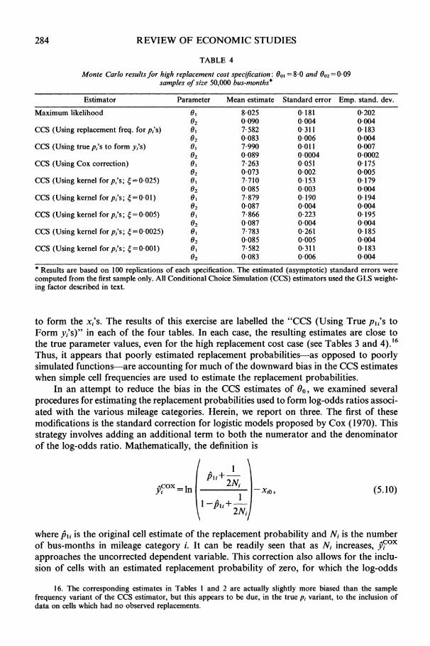