A Simulation-Based Digital Twin for Model-Driven He alth ... · A Simulation-Based Digital Twin for Model-Driven He alth Monitoring and Predictive Maintenance of an Automot ive

A Simulation-Based Digital Twin for Model-Driven Health Monitoring and Predictive Maintenance of an Automotive Braking

System

Ryan Magargle1 Lee Johnson1 Padmesh Mandloi1 Peyman Davoudabadi1 Omkar Kesarkar1 Sivasubramani Krishnaswamy1 John Batteh2 Anand Pitchaikani2

1ANSYS Inc., USA, {ryan.magargle,lee.johnson,padmesh.mandloi, mohammad.davoudabadi, omkar.kesarkar, sivasubramani.krishnaswamy}@ansys.com

2Modelon Inc., USA, {john.batteh,anand.pitchaikani}@modelon.com

Abstract This paper describes a model-driven approach to

support heat monitoring and predictive maintenance of an automotive braking system. This approach includes the creation of a simulation-based digital twin, or numerical model, that combines different modeling formalisms into an integrated model of the braking system that can be used for monitoring, diagnostics, and prognostics. The paper provides an overview of the basic models including Modelica models, reduced order models for various key components of the system model, and controls and sensor models. The Modelica models are implemented in the ANSYS Simplorer simulation to leverage existing modeling work and connections with other ANSYS finite element software to utilize reduced order models. The simulation results include both baseline results for the system and the results of injecting failures into the system for monitoring and predictive maintenance.

Keywords: digital twin; electronics; electromagnetics; hydraulics; pneumatics; braking system; automotive; FEA;

1 Introduction Beyond the challenges of developing complex products, companies are increasingly seeking to monitor and manage the performance of those products in operation to improve safety, performance, and customer satisfaction (GE, 2016; Siemens, 2016). Model-based approaches and physics simulation are powerful components of creating a digital twin of a physical asset in operation-- a simulated replica of the asset that is used to diagnose anomalies in the performance of the asset and for predicting the state of health and remaining useful life of that asset. These insights can subsequently be used with machine learning algorithms to optimize operational downtime, trigger pre-emptive maintenance, and mitigate costly failures (Prytz, 2014). The work shows multi-domain system simulation modeling that can be used with a

variety of machine learning analytics engines, such as PTC Thingworx (PTC, 2016), which are not discussed in detail here.

The automotive industry produces millions of vehicles operating in diverse conditions and require periodic maintenance to replace worn components and address faulty conditions. Current vehicle health management practices rely heavily on data science, which has become quite powerful (Holland, 2010); however, the role of engineering and physics in these practices is limited and are included only in the form of simplified relations, material data, etc. This approach therefore has limited the applicability of health management systems to diagnostics and managed maintenance for a few automotive components and systems. The need for higher value capabilities like prognostics for critical components and systems, e.g. engine, exhaust aftertreatment, and safety, are driving the evolution of vehicle health management.

Digital twins offer automotive manufacturers an enhanced ability to diagnose anomalous conditions and predict remaining useful life of degradable components, thereby improving owner safety and satisfaction.

An approach of combining physics-based modeling techniques (0-D, 1-D, 3-D) at the system level is applied to create a digital twin for predicting brake pad wear in a conventional passenger vehicle. Versus relying solely on physical measurements, a simulation-based approach produces a high-fidelity model that can be used to predict brake pad wear, given a set of operating conditions. Further, the physics-based models are subjected to failure modes that can produce abnormal brake pad wear and unsafe conditions, and simulated to observe the sensor signatures that will subsequently aid in improving the diagnosis and mitigation of unsafe or undesirable conditions in the vehicle.

DOI10.3384/ecp1713235

Proceedings of the 12th International Modelica ConferenceMay 15-17, 2017, Prague, Czech Republic

35

2 Modeling Overview This section of the paper provides an overview of the integrated braking system model and the individual model components.

2.1 Integrated Model The integrated braking system model in Simplorer (ANSYS, 2016) with all subcomponents is shown in Figure 1. Simplorer offers a system modeling and integration platform that supports multiple modeling formalisms, including Modelica based on the OPTIMICA Compiler (Modelon AB, 2016) from Modelon, system models using other formalisms like VHDL-AMS, reduced order models, and controls. The power converter is on the left, followed by the electromagnetic solenoid actuator, pneumatic and hydraulic braking system, and vehicle dynamics (including the speed sensor), and brake wear model. The controller is on the top, providing feedback from the measured speed and slip output to the command signal input to the power converter.

Figure 1. The full system schematic including electrical, pneumatic, hydraulic, mechanical and control logic components.

2.2 Reduced Order Modeling (ROM) Several reduced order models generated from detailed 3-D simulations are used in this system simulation to capture component effects that might be difficult to describe with closed form solutions. The electromagnetics models of the ABS valve solenoid actuator, the magnetic wheel speed sensor, and the mechanical brake wear are all based on finite element numerical models to capture the relevant nonlinear physics.

The basis of all three reduced order models is a lookup table based on the numerical model outputs versus specified input variables. The electromagnetic solenoid actuator uses the lookup table to capture the dependence of the magnetic flux linkage vs current and magnetic force versus displacement (Woodson, 1968). The magnetic wheel speed sensor has a lookup table that represents the angular displacement of the magnetic fields on the sensor surface, in degrees, versus the position of the wheel sensor. The brake pad wear model lookup table represents the wear rate, in

mm, of the pad surface vs pad normal pressure and wheel speed.

The following sections will describe all of the major sub-component models and reduced order modeling implementation from each of the finite element numerical models.

2.3 Model Components This section of the paper details the physical, control system, and sensor components that comprise the braking system model.

2.3.1 Electronics

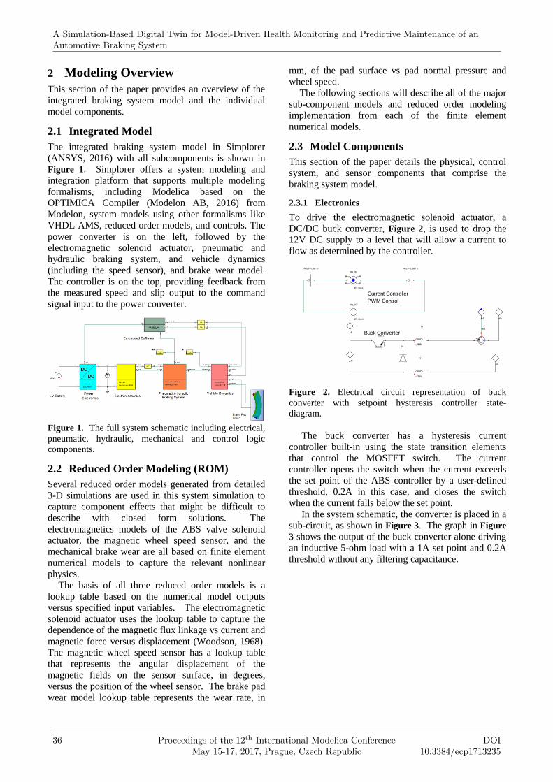
To drive the electromagnetic solenoid actuator, a DC/DC buck converter, Figure 2, is used to drop the 12V DC supply to a level that will allow a current to flow as determined by the controller.

Figure 2. Electrical circuit representation of buck converter with setpoint hysteresis controller state-diagram.

The buck converter has a hysteresis current controller built-in using the state transition elements that control the MOSFET switch. The current controller opens the switch when the current exceeds the set point of the ABS controller by a user-defined threshold, 0.2A in this case, and closes the switch when the current falls below the set point.

In the system schematic, the converter is placed in a sub-circuit, as shown in Figure 3. The graph in Figure 3 shows the output of the buck converter alone driving an inductive 5-ohm load with a 1A set point and 0.2A threshold without any filtering capacitance.

Current ControllerPWM Control

Buck Converter

VA

VB

I_d

VP

VN

IGBT1

D1L=1uH

L1

A

AM1

AM1.I<=I_set - D AM1.I>=I_set + D

SW_OFF

SET: S1:=0

SW_ON

SET: S1:=1

L=1uH

L2

A Simulation-Based Digital Twin for Model-Driven Health Monitoring and Predictive Maintenance of anAutomotive Braking System

36 Proceedings of the 12th International Modelica ConferenceMay 15-17, 2017, Prague, Czech Republic

DOI10.3384/ecp1713235

Figure 3. Power converter subcircuit output current results for 5 ohm, 0.1 mH load.

2.3.2 Electromagnetics

The DC/DC power converter is used to drive the electromagnetic solenoid actuator that the ABS controller uses to bypass brake actuator and vary braking pressure. To calculate the force generated by the current flowing through the solenoid coil, including any nonlinear effects from the steel and airgap displacement, not amenable to closed form solution, a 2-D axi-symmetric magnetostatic model is created in Maxwell2D (ANSYS, 2016), as shown in Figure 4. Maxwell2D uses the finite element method to calculate the magnetic field (Chari, 1977), as seen in Figure 5, and uses the virtual work method (Fu, 2004) to calculate the force on the moving armature. The winding is shown as a solid object, but it represents 400 turns of copper wire in this model.

Figure 4. 2-D model of electromagnetic solenoid actuator

Figure 5. Magnetic flux density and field lines within the solenoid for a DC current excitation of 1.8 Amps through 400 turns.

The airgap and current are parametrically varied and the force and inductance are calculated to create a table of results, as seen in Figure 6.

Buck Converter12V Battery

Current Setpoint

+

V

VM1

DC

DCVA

VB

VP

VN

I_set

Chopper

Buck_1A23XD9

E1

EMF=12

CONST

5ohm

0.1mH

Session 4A: Automotive I

DOI10.3384/ecp1713235


37

Figure 6. Force vs airgap curves for different current excitations.

The result of the parametric sweep creates a multidimensional lookup table of current, flux linkage, displacement, and force. Maxwell automatically creates a circuit element that uses dependent sources and a lookup table to relate the electrical input energy and mechanical output energy, where losses can be lumped and made external to the component, as in Figure 7 (Woodson, 1968).

Figure 7. Equivalent circuit of electrical solenoid actuator using the lookup table results from the finite element simulation.

Together with the rest of the system circuit, the electrical actuator is implemented with an icon, containing all of the complexity of Figure 7. The circuit model is connected with mechanical elements, such as the restoration spring and mechanical damping, as seen in Figure 8.

Figure 8. System model implementation of actuator with mechanical elements such as spring and mechanical damping loss connected externally.

2.3.3 Brake pad

A detailed 3-D model consisting of brake rotor, hub, and pads was constructed to predict brake pad wear as a function of rotor velocity and pressure applied to the brake pads, shown in Figure 9 as a meshed geometry simulated using nonlinear structural finite element analysis (FEA) within ANSYS Mechanical (ANSYS, 2016).

Figure 9. Meshed 3-D geometry of the rotor discs, rotor vents, hub, and pad assembly.

Brake pad wear is calculated as part of the FEA

solution using the Archard Wear Model (Archard, 1980), shown in generalized form in Figure 10.

Figure 10. Generalized Archard Wear Model used by ANSYS Mechanical.

During the FEA simulation, constant pressure is applied on the outer faces of the two brake pads to interact with the rotor, spinning at a constant velocity. Boundary conditions constrain brake pad movement in the direction normal to the rotor, whereas in more detailed studies the motion would be determined by the brake calipers and guide pins. The simulation produces a wear rate of the brake pads as a function of the applied pressure and rotor velocity, shown in Figure 11.

+

− DECE Look-up

Table

Input: ia, pos

Output: λa, F

FA

posia

λa

F

iapos

S

Magnetic Valve (ECE)

0 0 0

VA

VB

F_valve

S_valve

S+

F

S_TRB1

Current1_N1

Current1_N2

ArmForce_N1

ArmForce_N2

SPRING_TRB1

S+S_Airgap

LIMIT_TRB1

F_mag1

FF_TRB1



DOI10.3384/ecp1713235

Figure 11. Wear rate on the brake pad for a constant applied pressure and rotor velocity.

Using distributed computing, the FEA simulation

was performed for a number of combinations of pressure applied on the brake pads and rotor velocity to produce a response surface of wear rate at a selected location on the surface of the brake pad, illustrated in Figure 12. This response surface model was then encapsulated as a Functional Mock-up Unit (FMU) and connected to the speed and force inputs produced by the vehicle dynamics and ABS subsystems in the Simplorer system model. The output of this model can be integrated, using a standard integration block to measure accumulated wear.

Figure 12. Response surface model of brake pad wear versus brake pressure and rotor velocity.

2.3.4 Braking System

Leveraging the latest capability in Simplorer for modeling with Modelica, the braking system is modeled natively in Modelica as a pneumatic and hydraulic system using the Pneumatics Library and Hydraulics Library (Modelon AB, 2016). The model shown in Figure 13 consists of a pneumatic system for the brake booster (a) and the hydraulic system (b) for the brake actuation.

a) Assembled braking system

b) Pneumatic brake booster

c) Hydraulic brake actuation

d) Modelica implementation in Simplorer

Figure 13. Pneumatic and hydraulic braking system model


DOI10.3384/ecp1713235


39

Based on the brake pedal input from the driver, the models calculate the resulting caliper pressure that is provided to the vehicle model for use in calculation of the brake torque. The ABS valve that modulates the brake pressure based on the electromagnetic force actuation is shown in Figure 13b.

2.3.5 Vehicle Dynamics

The vehicle is modeled in Modelica with basic longitudinal dynamics considering a lumped vehicle mass and a simple single wheel approach. The Modelica model in Simplorer is shown in Figure 14. The tire dynamics include the effects of slip via the Pacejka magic tire formula (Pacejka, 1993). The vehicle model takes the drive torque and the brake caliper pressure and calculates the resulting vehicle response and wheel conditions, including wheel speed and slip. The wheel speed is passed to the model of the wheel speed sensor for slip estimation, and the vehicle speed is provided to the controller.

Figure 14. Vehicle dynamics model implemented in Modelica in Simplorer

While the vehicle dynamics considered are fairly simple, the native Modelica capability in Simplorer allows for more complex models to be included to capture higher frequency dynamics. For example, models from the Vehicle Dynamics Library (Modelon AB, 2016) can be integrated to capture higher fidelity chassis dynamics and also more detailed tire dynamics and tire/ground interactions.

2.3.6 Controls

Shown in Figure 15, control of the ABS valve is implemented as a state machine in ANSYS SCADE Suite, a model-based environment for developing embedded software, often for applications where safety is critical (ANSYS, 2016).

Figure 15. ABS control as a state diagram which modulates the activation of the ABS valves.

During a braking event, the control algorithm uses

the measured vehicle speed and calculation of wheel to determine which braking mode to activate. If vehicle speed is below a low-speed threshold or if the calculated wheel slip is less than a minimum value, an unmodulated braking command is sent to the ABS actuator. If vehicle speed is above the low-speed threshold, the controller sends a modulated command signal to the ABS actuator when wheel slip exceeds the established threshold.

Using SCADE code generation, the model-based representation of the controller was transformed into C code and compiled into an FMU, shown in Figure 16. The FMU was directly integrated into the braking system model within ANSYS Simplorer. Simulated braking tests were applied to the system model to validate the operation of the control algorithm under various conditions. Figure 17 shows the modulation of the ABS during the application of full braking on dry pavement at a speed of 20 m/s.

Figure 16. Generated C code for the ABS controller, encapsulated as a Functional Mock-up Unit.

vehicleVelocity

abs_on_vel

Iref

slip

gain

activate

slip_on_val

slip_off_val

vehicle_velocity

abs_on_vel

slip

ctrl_gain

braking

slip_ON

slip_OFF

ctrl_sig

controller



DOI10.3384/ecp1713235

Figure 17. Simulated results of maximum braking applied on dry pavement at 20 m/s.

2.3.7 Speed sensor

The sensor for measuring the wheel speed is an anisotropic magnetoresistive sensor (Lenz, 1990). As the teeth on a magnetic tone ring pass by the sensor, the changes in the direction of the magnetic field relative to the current flow in the sensor cause changes in the resistance of the modules, as seen in Figure 18 and Figure 19.

Figure 18. Magnetoresistive material, showing a varying resistance as an external magnetic field angle of incidence changes vs the direction of current flowing through the material.

The variation in resistance follows a squared sinusoidal dependence on angle from -90deg to 90deg shown in Figure 18, according to the relation (McGuire, 1975):

)(cos)( 2 tRRtR o α∆+= (1)

Taking advantage of this variation, the modules are

arranged in Wheatstone bridge configuration so measurable voltage changes result on their output. The change in direction of the magnetic field due to the variable reluctance of the teeth as they pass is calculated by the Maxwell3D finite element program (ANSYS, 2016), as seen in Figure 19 using a 2-D view to visualize the magnetic flux lines. The flux lines can be seen originating from a permanent magnet and then linking with the nearest tooth creating an angle relative to the face of the magnet and sensor.

Figure 19. Magnetic flux bending as the tone ring teeth move past the stationary sensor, measuring flux direction as points, P1 and P2.

The two sets of resistive sensor modules are at each point, P1 and P2, as shown in Figure 19. The resistive Wheatstone bridge shown in Figure 20 has equal resistors in opposing positions within the bridge.

Figure 20. Magnetoresistor bridge with matching resistors placed in opposite positions.

With this arrangement, the output voltage, Vout, can be seen to change with a change in direction leading to incremental changes in resistance, dR, as the following:


DOI10.3384/ecp1713235


41

+−

+=−= −+

31

3

42

4

RR

R

RR

RVVVV inoutoutout (2)

( )tdRRRR o +== 41 (3)

( )tdRRRR o −== 32 (4)

where from (1),

)(cos)( 2 tRtdR α∆= , (5)

( )tRItdRR

V

R

tdRVV o

o

in

oinout α2cos)(

)( ∆=

=

=∴ (6)

So it can be seen that the output voltage would be

equal to the current, Io, through the nominal resistance, Ro, times the change in the resistance. ∆R is the maximum possible change in resistance, Ro is the nominal resistance, and α(t) is the field angle relative to the current flow. If there is no change in resistance, the output voltage is zero, as expected from a balanced bridge configuration.

To model the resistor bridge in a circuit simulation using Simplorer (ANSYS, 2016), the equation for the resistance in Figure 18 and (1) is used. Ro is given as 1200 ohm and ∆R is given as 0.02 ohm. α is measured for all positions of the sensor in the FEA simulation at both P1 and P2, which are used for R1, R4 and R2, R3 respectively. The average magnetic fields in the volumes of P1 and P2 are used according to the following equation for α:

=

∫∫−

dVH

dVH

x

y1tanα (7)

Therefore, for any given velocity of the tone ring,

the position can be instantaneously measured and evaluated against a precomputed table of values of α, for P1 and P2, for different tone ring positions. This method excludes any dynamic eddy currents.

In the circuit, this table is represented by a lookup table model with the angle position as an input and the corresponding value of α at P1 and P2, Figure 21.

Figure 21. Circuit model of finite element based lookup table, with tone ring position as an input and magnetic field angle measured at P1 and P2.

The values of α are then passed to an equation block where the resistance in (1) is calculated for R1, R2, R3, and R4, as shown in Figure 22.

Figure 22. Circuit model equations for the value of the magnetoresistors as the field angles change.

These computed values of resistance are then linked to a resistor bridge, with the value of each resistance being fed from each corresponding output of the equation block, Figure 23 and Figure 24.

Figure 23. Circuit magnetoresistor bridge model, graphically using resistance values calculated from the equation block in Figure 22 with wire connections.

Figure 24. Resistor model properties obtaining resistance from the equation block.

The output of this resistor bridge generates a voltage on the order of 30µV for a wheel rotation of 600rpm, so this measurement voltage is passed onto a



DOI10.3384/ecp1713235

comparator amplifier which, using a 5V, ground referenced input, generates a 10V bipolar waveform, Figure 25.

Figure 25. Comparator amplifier electrical circuit and the output before and after amplification.

This waveform is then used in an encoder that counts the zero crossings to estimate the speed of rotation, using state transition blocks, as seen in Figure 26.

Figure 26. Circuit state-diagram containing the zero-crossing logic to count the duration of teeth passing the sensor to derive the wheel rotation speed.

The state diagram has a transition to catch the signal zero crossing from positive to negative and a state transition to catch the zero cross from negative to positive. The time between them is the transit time of the tooth, which is used to calculate the instantaneous rotation speed, since the angular spacing of the teeth is fixed at 15 deg. If the speed slows down to near zero, the encoder also slows down in its response, so it has several timeout loops that estimate the speed as zero if the time between zero crossings exceeds a user defined threshold, 50ms in this case.

All of these sensor components are placed into sub-circuits, Figure 27.

Figure 27. Circuit representation of speed sensor with resistor bridge, amplifier, and encoder.

As indicated in Figure 27, the vehicle model rotation wheel speed is taken as an input, integrated to create an angle for the tone ring which is passed to the magnetoresistor bridge. The resistor bridge signal is sent into the amplifier, which is connected to the encoder, which outputs the estimated wheel speed. Any faults in the tone ring or other subcircuits will create estimated wheel speed errors compared to the actual wheel speed.

The nominal operation of the speed sensor is shown in Figure 28 using a 600rpm sinusoidal varying input speed. The waveform varies between 20 rpm and 600 rpm, some stepping can be seen in the encoder output at low input speeds since the encoder counter also slows.

Figure 28. Encoder response (bottom) compared to input 600rpm sinusoidal speed input (top).

3 Simulation Results With all of the component models represented in the system, several results can be obtained. The simulation results of the system are very useful for analyzing failure data, since in many real measured datasets this type of data can be difficult to obtain, especially for corner cases. This failure data is very useful for training analytics to enable predictive maintenance and enhanced failure analysis. Simulation results in this example will be obtained with the integrated model in Figure 1 for normal ABS operation and abnormal ABS operation break wear, and sensor waveform signature for normal and abnormal sensor operation.

(Vin == 0.0)SET: Speed:=7.5 / (Time - Tprev)SET: WavePeriod:=Time-TprevSET: Tprev:=Time

SET: Tprev0:=time

(Vin == 0.0)

SET: Speed:=0

(time-Tprev0) > 0.05 (time-Tprev) > 0.05

SET: Speed:=0

(Vin == 0.0)

(Vin == 0.0)


DOI10.3384/ecp1713235


43

3.1 Baseline System Performance The baseline performance is shown in Figure 29 for a 3 second braking event from 20 m/s to a complete stop including normal ABS activation.

Figure 29. Normal vehicle telemetry results for a full stop from 20 m/s using normal ABS activation.

The amount of brake wear that results, measured in mm, is shown in Figure 30.

Figure 30. Brake wear for normal stopping condition with ABS activation.

3.2 Fault Injection: Disconnected ABS Controller

In the first fault scenario, the controller fails and is disconnected from the circuit. In this case, the ABS activation does not occur. The vehicle telemetry results in this scenario can be seen in Figure 31 for the same braking scenario from 20 m/s to a complete stop.

Figure 31. Vehicle telemetry results for a full stop from 20 m/s with abnormal ABS failure.

The brake wear that results in the absence of the ABS activation can be seen in Figure 32.

Figure 32. Brake wear for abnormal stopping condition without ABS activation.

It can be seen that with ABS activation there is a cumulative brake wear for this single braking event of 6.25x10-10 mm. Without ABS, the brake wear is 1.38x10-10 mm. There is less wear in the absence of ABS since the wheel spends more time locked to the brake pads, which also causes the vehicle to spend more time coming to a complete stop. The cumulative wear numbers are very low, since only a single braking event is being investigated.

3.3 Fault Injection: Broken Sensor In the second scenario, the speed sensor tone ring is modeled with missing teeth (Obrochta, 2015), as seen in Figure 33, and causes the sensor to misread the wheel speed.

For this simulation, the first second of braking behavior is investigated for a sensor signature and the effect on ABS behavior. Figure 34a shows the normal sensor behavior. Figure 34b shows the effect of missing one tooth, and Figure 34c shows the effect of missing two non-adjacent teeth.

Figure 33. Tone ring mechanical failure with missing teeth.



DOI10.3384/ecp1713235

a) Vehicle telemetry results for the first second

with no missing teeth.

b) Vehicle telemetry results for the first second

with one missing tooth

c) Vehicle telemetry results for the first second with two non-adjacent missing teeth on the tone ring.

Figure 34. Vehicle telemetry results showing the effect of missing teeth

As teeth go missing from the tone ring, the wheel speed and slip measurements show intermittent dips. The dips represent a perceived reduction in speed since the time between zero crossings increases in the gap, resulting in an interpreted slowdown in speed. This perceived reduction in wheel rotation results in inadvertent ABS activation since it is interpreted as wheel slip since the vehicle speed does not change with it. The simulation can be run for any combination of missing teeth to create signatures leading to more accurate diagnosis of the ABS sensor and specific tone ring failure.

4 Summary and Future Work A model-driven simulation approach combining 0-D and 3-D physics-based models with controls to support heat monitoring and predictive maintenance for automotive braking stems was shown. These simulation-based digital twins are useful for providing inputs into analytics systems that support predictive maintenance for critical sub-systems, especially under abnormal operating conditions. As an example, the difference in wear rate was identified for normal conditions and abnormal conditions where the ABS controller becomes disconnected, to predict when maintenance is required on the braking system.

Simulation-based digital twin models are also useful for obtaining sensor signatures of the fault conditions needed to train machine learning algorithms that support advanced system diagnostics. These models are particularly useful for observing abnormalities and failures which cannot be observed easily in physical tests or in sufficient quantities to reliably train learning algorithms. In this paper, the unique ABS activation and speed-slip signals were recorded using simulation for several cases of mechanical failure of the teeth on the wheel sensor.

In order to realize these simulation-based digital twins, several methods of system, circuit, and reduced order modeling were shown using 3-D finite element analysis and 0-D multi-domain circuit simulation.

Future work will include more detailed physical models to support more vehicle operating scenarios and adding fault tree analysis with rigorous and automated scenario analysis for detailed root-cause and diagnostics analysis of brake wear. Further work can also be done to connect the simulation-based digital twin with real-time data from the vehicle and adding HMI (Human-Machine Interface) components to depict vehicle health management parameters (diagnostics, prognostics) to the driver.

Acknowledgements The authors gratefully acknowledge Leon Voss and Michael Sielemann for their work on the original braking system simulation model.

References ANSYS, Inc, Canonsburg, PA. (2016). Maxwell2D.

http://www.ansys.com.

ANSYS, Inc, Canonsburg, PA. (2016). Maxwell3D. http://www.ansys.com.

ANSYS, Inc, Canonsburg, PA. (2016). Mechanical. http://www.ansys.com

ANSYS, Inc, Canonsburg, PA. (2016). SCADE Suite. http://www.ansys.com.

ANSYS, Inc, Canonsburg, PA. (2016). Simplorer. http://www.ansys.com.


DOI10.3384/ecp1713235


45

GE, Boston, MA. (2016). How a ‘Digital Twin’ for physical assets can help achieve no unplanned downtime [Online]. Available: http://www.geglobalresearch.com/ impact/how-a-digital-twin-for-physical-assets-can-help-achieve-no-unplanned-downtime

J.F. Archard. Wear theory and mechanisms. Wear control handbook. Peterson MB, Winer WO, editors. New York ASME, 1980.

Donald C. Augustin, Mark S. Fineberg, Bruce B. Johnson, Robert N. Linebarger, F. John Sansom, and Jon C. Strauss. The SCi Continuous System Simulation Language (CSSL). Simulation, No 9, pp. 281–303, 1967.

M. V. K. Chari, Z. J. Csendes. Finite Element Analysis of the Skin Effect in Current Carrying Conductors. IEEE Transactions on Magnetics, 13(5): 1125-1127, September 1977.

Iain S. Duff and John K. Reid. An Implementation of Tarjan’s Algorithm for the Block Triangularization of a Matrix. ACM Transactions on Mathematical Software, 4(2):137–147, 1978. doi:

W.N Fu, P. Zhou, D. Lin, S. Stanton, Z.J. Cendes. Magnetic force computation in permanent magnets using a local energy coordinate derivative method. IEEE Trans. on Magnetics, 40(2): 683-686, 2004. doi: 10.1109/TMAG.2004.824774

S. Holland. Integrated Vehicle Health Management in the Automotive Industry. Health Management, Krzysztof Smigorski (Ed.). InTech, 2010. doi:10.5772/9889.J.E. Lenz. A review of magnetic sensors. Proc. of the IEEE, 78(6): 973-989, 1990. doi: 10.1109/5.56910

T. R. McGuire. Anisotropic magnetoresistance in ferromagnetic 3d alloys. IEEE Trans. Magn., 11(4), 1018–1038, 1975.

Modelon AB, Lund, Sweden. (2016). OPTIMICA Compiler Toolkit. http://www.modelon.com/products/optimica-compiler-toolkit/

Modelon AB, Lund, Sweden. (2016). Hydraulics Library. http://www.modelon.com/products/modelica-libraries/hydraulics-library/

Modelon AB, Lund, Sweden. (2016). Pneumatics Library. http://www.modelon.com/products/modelica-libraries/pneumatics-library/

Modelon AB, Lund, Sweden. (2016). Vehicle Dynamics Library. http://www.modelon.com/products/modelica-libraries/vehicle-dynamics-library/

Eric Obrochta. (2015, Dec. 5). Saturn S series - unwanted ABS activation at all speeds. [YouTube video]. Available: https://www.youtube.com/watch?v=oGwyrLxtaNY&t=368s. Accessed Dec. 15, 2016.

Pacejka, H.B., and Bakker, E. (1993): The Magic Formula tyre model. Proceedings of 1st Colloquium on Tyre Models for Vehicle Analysis, Delft 1991, ed. H.B. Pacejka, Suppl. Vehicle System Dynamics, 21, 1993.

PTC, Needham, MA. (2016). Thingworx Analytics. http://www.ptc.com/internet-of-things/analytics.

R. Prytz. Machine Learning Methods for Vehicle Predictive Maintenance using Off-Board and On-Board Data. Halmstad University Dissertations, No. 9, 2014.Siemens, Munich, GmBH (2016). The Digital Twin [Online].

Available: https://www.siemens.com/customer-magazine/en/home/ industry/digitalization-in-machine-building/the-digital-twin.html

H. H. Woodson and J. R. Melcher. Electromechanical Dynamics: Part I: Discrete Systems. New York, NY: John Wiley & Sons, 1968.



DOI10.3384/ecp1713235

Documents

A Simulation-Based Digital Twin for Model-Driven He alth ... · A Simulation-Based Digital Twin for Model-Driven He alth Monitoring and Predictive Maintenance of an Automot ive