A Simplified Statistical Model for the Geomagnetic Field

1. INTRODUCTION

One of the most useful assumptions in paleomagnetism isthat the geomagnetic field is on average close to that of a geo-

Timescales of the Paleomagnetic FieldGeophysical Monograph Series 145Copyright 2004 by the American Geophysical Union10.1029/145GM08 101

A Simplified Statistical Model for the Geomagnetic Fieldand the Detection of Shallow Bias in Paleomagnetic

Inclinations: Was the Ancient Magnetic Field Dipolar?

Lisa Tauxe

Scripps Institution of Oceanography, La Jolla, California

Dennis V. Kent

Department of Geological Sciences, Rutgers University, Piscataway, New Jersey andLamont-Doherty Earth Observatory, Palisades, New York

The assumption that the time-averaged geomagnetic field closely approximates thatof a geocentric axial dipole (GAD) is valid for at least the last 5 million years andmost paleomagnetic studies make this implicit assumption. Inclination anomaliesobserved in several recent studies have called the essential GAD nature of theancient geomagnetic field into question, calling on large (up to 20%) contributionsof the axial octupolar term to the geocentric axial dipole in the spherical harmonicexpansion to explain shallow inclinations for even the Miocene. In this paper, wedevelop a simplified statistical model for paleosecular variation (PSV) of the geo-magnetic field that can be used to predict paleomagnetic observables. The model pre-dicts that virtual geomagnetic pole (VGP) distributions are circularly symmetric,implying that the associated directions are not, particularly at lower latitudes. Elon-gation of directions is North-South and varies smoothly as a function of latitude(and inclination). We use the model to characterize distributions expected fromPSV to distinguish between directional anomalies resulting from sedimentary incli-nation error and from non-zero non-dipole terms, in particular a persistent axialoctupole term. We develop methodologies to correct the shallow bias resulting fromsedimentary inclination error. Application to a study of Oligo-Miocene redbeds incentral Asia confirms that the reported discrepancies from a GAD field in thisregion are most probably due to sedimentary inclination error rather than a non-GAD field geometry or undetected crustal shortening. Although non-GAD fields canbe imagined that explain the data equally well, the principle of least astonishmentrequires us to consider plausible mechanisms such as sedimentary inclination erroras the cause of persistent shallow bias before resorting to the very “expensive”option of throwing out the GAD hypothesis.

centric axial dipole (GAD). The GAD model is a specific,testable hypothesis, which for the past few million years pro-vides an excellent fit to global data such that the largest non-GAD contribution is generally found to be no more than about5% of GAD (e.g. Opdyke and Henry [1969]; Merrill andMcElhinny [1977]; Schneider and Kent [1988]; Gubbins andKelly [1993]; Kelly and Gubbins [1997]; Quidelleur et al.[1994]; Johnson and Constable [1995]; Johnson and Con-stable [1998]; Carlut et al. [2000]).

It is difficult to test the GAD hypothesis in ancient timesowing to plate movements, rock deformation and remagneti-zation. Nevertheless, the inescapable conclusion from a vari-ety of paleomagnetic data and analysis techniques is that thereis often a strong bias toward shallow inclinations that appearsinconsistent with a GAD model for the ancient time-averagedgeomagnetic field (e.g., Kent and Smethurst [1998], Westphal[1993], Si and Van der Voo [2001]). There are many potentialcauses for mean directions and distributions that are biasedshallow. Given the fundamental utility of the GAD assumptionin paleomagnetism, alternative mechanisms deserve a closerlook. In this paper we will consider depositional inclinationerror, especially in detrital hematite, as a better explanation formany of the discrepant observations.

In this paper, we will examine the evidence for inclinationanomalies in the Central Asian redbed sediments and explorethe possible explanations. Then we will develop a simple sta-tistical model for paleosecular variation which predicts dis-tributions of geomagnetic vectors in agreement with thecurrently available data sets. The model can be modified toinclude arbitrary non-zero gauss terms and we investigate theeffect of adding an arbitrary amount of non-zero axial octu-pole on the predicted distributions. We then consider the con-sequences of sedimentary inclination error on distributionsof directions and propose two methods for detecting and cor-recting for the resulting shallow bias.

2. INCLINATION ANOMALIES IN CENTRAL ASIANRED BEDS

Paleomagnetic poles obtained from globally distributedlocations will tend to average out non-dipole field contribu-tions; hence globally averaged paleopoles should reflect mainlythe GAD field. These poles are often used to predict directionsat specific locations. The difference between the predictedand observed directions could be caused by local non-dipolefield effects, local artifacts caused by rock deformation, orby magnetic recording biases. Paleomagnetists typicallyassume that the geomagnetic field has been essentially GADin order to estimate a reference pole for a given plate at thedesired time (e.g., Irving [1964]). If the rotation parameterslinking various plates are known, then these reference poles

can be used to predict directions expected from a GAD fieldat any place on any linked plate. An updated compilation ofpaleopoles for the Atlantic-bordering continents for 0-200Ma shows very good agreement with the GAD model, withonly a small (~3%) axial quadrupolar contribution [Besse andCourtillot, 2002]. Despite general agreement, comparison ofpredicted directions with those observed reveals a persistentshallow bias in Cenozoic paleomagnetic directions from sed-iments of Central Asia (see, e.g., Thomas et al. [1993]; Chau-vin et al. [1996]; Cogné et al. [1999]; Si and Van der Voo[2001]; Dupont-Nivet et al. [2002]; Gilder et al. [2003]).

Non-GAD geomagnetic fields, in particular axial octupo-lar fields ( ), have been called on to explain the CentralAsian inclination anomalies (e.g., Thomas et al. [1993]; Chau-vin et al. [1996]; Van der Voo and Torsvik [2001]; Si and Vander Voo [2001]; Dupont-Nivet et al. [2002] ). The logic accord-ing to, for example, Si and Van der Voo [2001], is that thereference poles are largely based on results from the UK andNorth America. A non-zero axial octupolar contribution withthe same sign as the dipole makes directions in mid-north-ern latitudes shallower than expected from a GAD field. Thesedirections, when converted to paleomagnetic poles will be“far-sided.” If this reference pole is then used to predict direc-tions in Asia, the predicted directions will be too steep. Theeffect is amplif ied by the fact that the actual directionsobserved in Asia in the same octupolar field will be shallowerthan expected from GAD. Typical contributions of calledfor are between 10 and 20% of the average axial dipole.

While most studies attribute the observed inclination shal-lowing to non-GAD geomagnetic fields, there are alternativeinterpretations. Cogné et al. [1999] attributed the effect to alarge degree of tectonic shortening. Recently, sedimentaryinclination error (either by compaction or by initial depositionalprocesses) has gained favor as a possible explanation for theeffect (e.g., Gilder et al. [2001]; Dupont-Nivet et al. [2002];Tan et al. [2003]; Gilder et al. [2003]).

The overwhelming majority of the paleomagnetic data fromCentral Asia come from red beds whose remanence is attrib-uted to detrital hematite by the authors. Tauxe and Kent [1984]studied natural (modern) and laboratory redeposited sedi-ments with detrital hematite. Results from their redepositionexperiments are shown in Figure 1a. These data demonstratea pronounced bias toward shallow inclinations that follow the“inclination error formula” of King [1955]:

(1)

where Io and If are the observed and applied field inclina-tions, respectively, and f is an empirical coefficient (here calledthe “flattening factor”), estimated to be about 0.55 (dashedline in Figure 1a) in these particular sediments.

tan( ) tan( )o fI f I=

03g

03g

2 STATISTICAL FIELD MODEL AND SHALLOW INCLINATIONS

Gilder et al. [2003] compiled paleomagnetic data for Ceno-zoic and Mesozoic sediments and basalts from Central Asianorth of the Tibetan plateau. We replot their red bed data com-pilation as observed inclinations versus predicted inclinationsfrom Besse and Courtillot [2002] as solid dots in Figure 1.Data from igneous rocks are shown as open circles. Theoret-ical curves for inclination error with f = 0.4 and 0.6 are shownon Figure 1b as dashed lines. In general, the observed incli-nations from the sediments fall well below the expected val-ues. Data from basaltic units in the same compilation do notdisplay a shallow bias as shown also by Bazhenov and Miko-laichuk [2002]. These data show conclusively that the sedi-mentary units are shallower than the basaltic data; henceGilder et al. [2003] strongly argue for inclination error as acause of the inclination anomaly.

Based on the predicted and observed inclinations shown inFigure 1b, it is reasonable to interpret the shallow inclina-tions from Central Asian sediments as resulting from sedi-mentary inclination error. However, non-GAD field geometryor crustal motion inconsistent with geological observationshave been called upon as plausible explanations for shallowinclinations in many tectonic studies. Some means for dis-criminating among the various possibilities would be of gen-eral use.

We suggest in this paper that when inclination error occurs,it distorts the original distribution of directions in ways thatshould be distinguishable from the other mechanisms of incli-nation shallowing if the characterisics of the data set as awhole are considered. Before we begin to explore the effect ofinclination error on distributions of directions, we need tounderstand what distributions we might expect from secular

variation of the geomagnetic field itself. We therefore willfirst consider statistical paleosecular variation models capa-ble of predicting directions as a function of position on the sur-face of the Earth. We then will investigate the effect of non-zeroaverage octupolar components and finally we will character-ize the effect of sedimentary inclination error on directions.

3. PALEOMAGNETIC CONSTRAINTS ANDSTATISTICAL MODELS OF THE GEOMAGNETIC

FIELD

3.1. The Giant Gaussian Process

To predict the distribution of directions produced by pale-osecular variation of the geomagnetic field, we require a sta-tistical model to generate plausible sets of geomagnetic fieldvectors. A good starting point is the model of Constable andParker [1988] (hereafter CP88). This models the time varyinggeomagnetic field as a “Giant Gaussian Process” (GGP)whereby the gauss coefficients gl

m, , hlm (except for the axial

dipolar term, g10 and in some models also the axial quadrupole

term g20) have zero mean and standard deviations that are a

function of degree l. For l ≥ 2 these standard deviations aregiven by

(2)

where c/a is the ratio of the core radius to that of Earth and αis a fitted parameter. The parameters used in the model ofCP88 are listed in Table 1.

2 22 ( )

( 1)(2 1)lc a ll l

ασ /=+ +

TAUXE AND KENT 3

Figure 1. a) Observed inclination versus applied field determined for natural sediments with detrital hematite (data of Tauxeand Kent [1984]). Dashed line is for f = 0.55. b) Filled (sediments) and open (basalts) circles are observed inclination ver-sus predicted inclination from the APWP for Europe of Besse and Courtillot [2002] for data compiled by Gilder et al. [2003].Triangle is the magnetostratigraphic study of Gilder et al. [2001] to be discussed later. Dashed lines are the functiontan(Io) = f tan (If) for f = 0.4 and f = 0.6 (as labelled).

Many data sets show a persistent offset in equatorial incli-nations at least in reverse polarity data sets, consistent with asmall non-zero mean axial quadrupolar term ( ). We areignoring this effect in the present paper because the bias intro-duced by is negligible for the latitude of the Asian studiesand has not been considered as a possible explanation for theinclination anomalies observed there. Hence the version ofCP88 and other models discussed here are the “GAD” versionsin which the axial quadrupolar term has zero mean (e.g.,CP88.GAD).

The advantage of using a statistical model like CP88 is thatdistributions of directions with various non-zero gauss coef-ficients (such as the axial quadrupole or octupole term) canbe generated and compared with the paleomagnetic observa-tions and with other model predictions. One simply drawscoefficients for a field model from gaussian distributions withthe specified means and standard deviations and calculatesthe geomagnetic elements at a given position using the usualformulae (see Constable and Parker [1988] for details). Themain disadvantage of the CP88 model is that it fails to accountfor the observed variations in dispersion of the virtual geo-

magnetic poles (VGPs) calculated from directions as a func-tion of latitude (see e.g., McFadden et al. [1988]; Kono andTanaka [1995]; Constable and Johnson [1999]).

3.2. VGP Scatter as a Function of Latitude

McElhinny and McFadden [1997] (hereafter MM97) com-piled an updated paleosecular variation of recent lavas(PSVRL) database of directions from lava flows from the last5 million years that met their minimum acceptance criteria.They also estimated angular standard deviation of the scatterS of the VGPs with latitude. S (e.g., Cox [1969]) is defined as

where N is the number of observations and ∆ is the anglebetween the ith VGP and the spin axis. In Figure 2 we show thevariation of VGP scatter as a function of latitude from thecompilation of MM97 as dots. One criterion for the PSVRLdatabase is that VGPs are rejected if they are more than 45°from the spin axis in order to avoid over-representation oftransitional data. The MM97 estimates of S also used a vari-able VGP colatitude cutoff as suggested by Vandamme [1994],which is an iterative process whereby the cutoff is found byθ = 1.85S + 5°. Cutoffs range from 25° at the equator to ~ 42°near the pole. Values of S based on trimmed data sets are heretermed S′. The predicted behavior of S′ from the CP88.GADmodel is shown as a dashed line in Figure 2.

The fact that VGP scatter increases with latitude has beenknown for decades (e.g., Cox [1962]). As pointed out byMcFadden et al. [1988] among others, gauss coefficients thatare asymmetric about the equator (those with l − m odd) con-tribute more strongly to the scatter in VGPs at high latitudethan those that are symmetric about the equator (those withl − m even). In order to improve the fit of the statistical pale-osecular variation model to their compilation of paleomag-netic observations, Quidelleur and Courtillot [1996] proposed

2 1 2

1

( 1) ( )N

ii

S N −

=

= − ∆∑

02g

02g


Figure 2. Estimated behavior of S′ from the data compilation ofMM97 (circles). The dashed line is the predicted behavior fromCP88.GAD, the dotted line is from CJ98.GAD and the heavy solidline is from TK03.GAD.

a variation on the CP88 model (hereafter QC96; see Table1). QC96 improves the fit by decreasing the variance in the

(symmetric) term and increasing the variance in the (asymmetric) terms relative to the CP88 model.

The most recent of the GGP type models is that of Con-stable and Johnson [1999] (hereafter CJ98). CJ98 attemptsto fit a compilation of lava flow data for the last 5 millionyears [Johnson and Constable, 1996]. The variant of theirmodel with zero average for the non-dipole terms is herecalled CJ98.GAD. Like QC96, CJ98 achieves an increase inhigh latitude VGP scatter by adding power to the asymmetricterms and decreasing power in the symmetric terms relativeto CP88. The prediction of the behavior of S′ with latitude ofCJ98.GAD (CJ98 as in Table 1 but with ) is shown asa dotted line in Figure 2. It does a good job of predicting theVGP scatter observed at high latitude, but under predicts scat-ter at lower latitudes. [We note that CJ98 was designed to fita different data compilation with more stringent VGP co-lat-itude cut-offs than MM97.]

3.3. A Simplified Giant Gausssian Process PaleosecularVariation Model

As discussed in the previous section and seen in Table 1,both QC96 and CJ98 manipulate the variance for each gaussterm separately to achieve a fit to the paleomagnetic obser-vations. We propose here a return to the simplicity of CP88,but modify it to properly account for the observed depend-ence of S on latitude. The latitudinal dependence of S can besimulated by having larger variance in the asymmetric gausscoefficients than in the symmetric ones. We therefore fitthe first order properties of the paleosecular variation database (average intensity and dispersion of VGPs with lati-

tude) with three parameters: the average axial dipole term, α as in Equation 2 and β defined as the ratio

for a given degree l. Because our understanding of the average field intensity

has changed recently (e.g., Selkin and Tauxe [2000]), noneof the statistical models fit the observed average intensity ofthe magnetic field very well, having an average field approx-imately equal to the present field. Selkin and Tauxe [2000]arrived at an average of approximately half that value, thatis, the virtual axial dipole moment (VADM) of the presentfield is approximately 80 ZAm2 [NB: Z = 1021] whereas theaverage VADM for the last five million years is approxi-mately 46 ZAm. We therefore set the value of the averageaxial dipole term ( ) to give the correct average VADM(see Table 1).

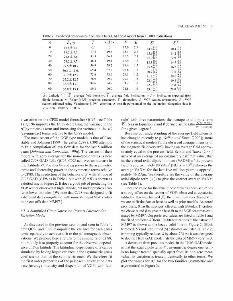
Once the value for the axial dipole term has been set, α hasa strong effect on the scatter of VGPs observed at equatoriallatitudes. Having changed , then, we must also change α ifwe are to fit the data at least as well as prior models. As notedpreviously, β has the strongest effect at high latitudes. Thereforewe chose α and β to give the best fit to the VGP scatter as esti-mated by MM97. Our preferred values are listed in Table 1 andthe fit of predicted S′ from 10,000 realizations to the dataset ofMM97 is shown as the heavy solid line in Figure 2. (Bothtrimmed (S′) and untrimmed (S) estimates are listed in Table 2;trimming typically reduces S by about 2°.) As it was designedto do, the TK03.GAD model fits the data of MM97 very well.

A departure from previous models in the TK03.GAD modelis that the axial dipole term ( ; asymmetric degree one term)is no longer treated specially apart from its non-zero meanvalue; its variation is treated identically to other terms. Weplot the values for for the two families (symmetric andasymmetric) in Figure 3a.

mlσ

01g

01g

01g

( odd)( even)

mlml

l ml m

σσ

− :− :

01g

02 0g =

12σ0

2σ

TAUXE AND KENT 5

3.4. Lowes Spectrum

Constable and Parker [1988] used the present (1980 Inter-national Geomagnetic Reference Field) as a guide for con-structing CP88. TK03 is constructed to f it thepaleomagnetic data for the last 5 million years instead. Tocompare the statistical behavior of model TK03.GAD withthe present geomagnetic field, we can calculate the powerRi in each degree (see, e.g., CP88) using the formula ofLowes [1974]:

for realizations of the model. We plot 25 so-called “Lowes-spectra” as thin dashed lines in Figure 3b. Averaging 10,000such realizations gives 95% confidence bounds on the modelwhich are plotted as heavy lines in Figure 3b. We also plotthe Lowes spectrum of the 1995 International GeomagneticReference Field as triangles. The fact that the spectrum of thepresent field lies at the very upper bound of realizations fromour statistical field model supports the contention of Hulotand Gallet [1996] that the present field is not a good guide forthe time-averaged field. In fact, it appears to be quite anunusual field state.

3.5. Predicted Distributions of Geomagnetic Vectors

Geomagnetic f ield vectors evaluated at various lati-tudes (λ) from 1000 realizations of model TK03.GADare shown in Plate 1a-d. We have plotted each realizationas a vector end-point in three dimensions where the RGB

color value reflects the contributions of North (red), East(green) and Down (blue). The same realizations are plot-ted along the principal directions of each cloud of pointsin Plate 1e–h. This projection is in many ways similar toan equal area projection of unit vectors centered on theprincipal direction, but we have included the intensityinformation as well.

The fact that we can simulate the full geomagnetic fieldvector allows us to predict the behavior of various parametersin frequent use in paleomagnetic studies, for example VGPsand virtual dipole moments (VDMs). We convert intensityvalues from 1000 realizations of TK03.GAD to Virtual AxialDipole Moments (VADM) and plot them against the VGP lat-itude of the associated direction (Figure 4). This plot exhibitsthe well known pattern from the geomagnetic field (e.g.,Tanaka et al. [1995]) of low VADMs associated with lowVGP latitudes. We note that while low paleointensities fre-

2 2

0

( 1)[( ) ( ) ]l

m mi l l

m

R l g h=

= + +∑


Figure 3. a) Variation of σ as a function of degree l for the symmetric (l − m even) and asymmetric (l − m odd) gauss termsfor model TK03.GAD (see Table 1). b) Power evaluated for representative realizations of the TK03.GAD (thin lines).95% confidence bounds derived from 10,000 realizations (heavy lines). Power spectrum of the IGRF for 1995 (dashed linewith triangles).

Figure 4. Vectors from realizations of TK03.GAD converted toVGP latitude and VADM for the equator (black) and the polar(lighter) observation sites.

TAUXE AND KENT 7

Plate 1. 1000 realizations of TK03.GAD projected as North (red), East (green) and Down (blue) components. Each dotis assigned the RGB color corresponding to the contributions from each component. a–d) All North axes are 40 µT long.(South, East and Up axis are the dashed lines. a) Equator, b) 30°N, c) 60°N, d) 90°N. e–h) Same data as a–d) but projectedalong the principal axis for each data cloud. All East axes are 20 µT. Axes labelled D′ are projections in the N–S plane look-ing along the expected direction at that latitude. e) Equator, f) 30°N, g) 60°N, h) 90°N.

Plate 2. a) Paleomagnetic directions of Oligo-Miocene redbeds from Asia [Gilder et al. 2001] in equal area projection (strati-graphic coordinates). b) Plot of elongation (heavy solid and dashed line) and inclination (dashed) as a function of unflat-tening by the parameter f in Equation 2. Elongation is E–W (N–S) when heavy line is solid (dashed) c) Plot of elongationversus inclination for the data in b) (solid) and for the TK03.GAD model (dashed). Also shown are results from 20 boot-strapped datasets. The crossing points represents the inclination/elongation pair most consistent with the TK03.GADmodel. d) Histogram of crossing points from 1000 bootstrapped datasets. The most frequent inclination (63°) is exactlythat predicted from the Besse and Courtillot [2001] European APWP. The 95% confidence bounds on this estimate are 56–69°.

quently occur with no directional deviations, all highly diver-gent directions are associated with low paleointensity. It istherefore perhaps inadvisable to identify “excursions” on thebasis of intensity records alone as excursions are by defini-tion intervals of deviant observation sites directions. Thelighter points in Figure 4 are from observations sites at thepole, while the darker (black) points are evaluated at theequator. There are many more divergent VGP latitudes in thepolar simulations than at the equator from the same fieldmodels. This model would predict therefore that excursionswould only rarely be observed globally, as deviant directions(defined as > 45° from the pole) are much more prevalent

at high latitude observation sites than at low latitude obser-vation sites in the model. Furthermore, our model suggeststhat the initial selection procedure of MM97 would excludemany observations from high latitude sites while including thecomparable observations from the same field state observedat low latitudes.

Because of the comparative dearth of intensity informationin routine paleomagnetic data sets, paleomagnetists rarelyconsider both direction and intensity in a single plot. Plotssimilar to those shown in Plate 1 cannot be constructed fromthe current data base with enough data points to fully char-acterize the vector distribution of the paleomagnetic field as


Figure 5. a) Paleomagnetic directions from the PSVRL database (see McElhinny and McFadden [1997]) compiled for lat-itude band 0–5° (N&S). Antipodes of reverse directions are used. The expected direction is at the star at the center of theequal area projection. Directions in the upper (lower) half are shallower (steeper) than expected and those to the right (left)are right-handed (left-handed). b) Same as a) but for 25–35° (N&S) latitude band. c) Same as a) but for 55–65° (N&S)latitude band. d) Same as a) but directions are from realizations of the TK03.GAD model evaluated at 0° latitude. Thereare the same number of directions as in a). e) Same as b) but for TK03.GAD model at 30° latitude. f) Same as c) but forthe TK03.GAD model at 60° latitude. g–i) The associated VGP positions of the model realizations of d–f) plotted in polarprojection (squares are the poles). The dashed circle is the 45° cutoff used as an initial cutoff for entry into the PSVRLdatabase. All VGPs outside of this circle would have been eliminated as “transitional” or “excursional”. Calculations ofS′ eliminate additional VGPs based on the variable cutoff criterion (see text).

a function of latitude. Instead, paleomagnetists generally plotdirectional data as unit vectors in equal area projection.

To illustrate how directions behave as a function of lati-tude, we plot directional data selected from the PSVRL data-base (downloaded in January 2002 from the NGDC website)for 10° latitude bands in Figures 5a–c. The directions are plot-ted (taking the antipodes of the reverse directions) projectedin equal area projections along the expected direction at eachlatitude from a GAD field (Hoffman [1984]). In addition to thecriteria of MM97 for inclusion in the database, we selected datawith demagnetization codes of 2 or better from sites with atleast 3 specimens and a κ of at least 100. We show realizationsof the same number of directions drawn from TK03.GAD(Figures 5d–f) and the associated VGPs (Figures 5g–i). Notethat no VGPs generated from TK03.GAD were trimmed inthese plots.

One observation from model TK03.GAD is that the simu-lated distributions of VGPs are circularly symmetric at all lat-itudes. [NB: The VGP distributions are not Fisherian sensustrictu as the distribution of latitudes is not exponential, hav-ing a low latitude tail.] Circular symmetry of VGPs implies thatthe corresponding distributions of directions cannot be sym-metric everywhere. In fact there is no essentially dipolar fieldstructure that can give rise to Fisher distributed directionseverywhere, so it is generally true that data sets of geomagneticfield directions would not be expected to be Fisher distrib-uted. Although this has long been suspected (e.g., Creer[1959]), it has been largely ignored in routine paleomagneticstudies (but see important exceptions by Baag and Helsley[1974], Kono [1997], Beck [1999], and Tanaka [1999]).

An immediate consequence of circularly symmetric VGPsis illustrated in Figure 6a in which we plot as small dots theVGP positions from field vectors drawn from TK03.GADevaluated at the sampling site (30°N; square). The geographicpole is indicated by the triangle. We also show a black ringof VGP positions at 60°N. This ring is converted to theexpected direction at the sampling site in Figure 6b with theexpected direction at the center of the diagram. The ring ofVGPs maps into an ellipse that is asymmetrical with a sig-nificant shallow bias. Because the most shallow directionsare associated with the low intensities (see e.g., Plate 1b andFigure 4), they do not bias the vector mean significantly.They do, however, bias the average inclination derived fromunit vectors (see Table 2). This inclination anomaly variesfrom zero at the equator to a maximum of about 3° at mid-latitudes and was predicted by Creer [1983] from a secularvariation model based on migrating radial dipoles. The essen-tial feature of Creer’s model was that VGP distributions arecircularly symmetric which is also a key feature of the typesof models considered here. Also noted by Creer [1983], theinclination anomaly has the same form as a non-zero con-tribution of the term. The magnitude of the effect is notlarge enough, however, to explain inclination anomalies of~20° under consideration here.

To characterize the elongation of the distribution of direc-tions derived from Fisher distributed VGPs as a function of lat-itude, Tanaka [1999] used the ratio of the 95% confidenceradii from Bingham statistics [Bingham, 1964; Bing-ham, 1974]. The radii of the Bingham ellipses are ultimatelybased on the eigenvalues of the “orientation matrix” T [Schei-degger, (1965)] which is defined as:

where xij are the ith component of the jth unit vector. The eigen-values τi and eigenvectors Vi reflect the shape and orienta-tion of the distribution of directions, respectively. For Fisherdistributions, the eigenvector V1 associated with the maxi-mum eigenvalue τ1 is coincident with the Fisher mean direc-tion. V2 and V3 are in the directions of the major and minoraxes of the Bingham confidence ellipse whose radii are relatedthrough a non-linear transformation to the eigenvalues. Herewe use the eigenvalues themselves and follow Tauxe [1998]who defined an elongation parameter E as the ratio τ2/τ3 toquantify the asymmetry in the distributions of directions seenin both the PSVRL dataset and the TK03.GAD model (Fig-ure 5a–f). (Note that this is different from the elongationdefined later by Beck [1999]). The elongation direction is thedeclination of V2or DV3.

31 32α α/

03g

TAUXE AND KENT 9

Figure 6. a) VGPs from geomagnetic vectors evaluated at 30°N(site of observation shown as square). The geographic pole is shownas a triangle. A set of VGP positions at 60°N are shown at the siteof observation [squares in (a)] converted from the black ring. b)Directions observed at the site of observation square in a) convertedfrom black ring of VGPs in a) which correspond to the VGP posi-tions at 60°N. These directions have been projected along expecteddirection at site of observation (triangle). Note that a circularly sym-metric ring about the geographic pole gives an asymmetric distri-bution of directions with a shallow bias.

We plot the behavior of elongation for the PSVRL datacompilation in approximately 20° latitude bands in Figure 7as solid dots. The dots are placed at the average latitude ofthe data set and the horizontal bars indicate the latitude win-dow from which the data were drawn. Also shown is the vari-ation of E predicted from TK03.GAD (triangles in Figure 7).E varies in the TK03.GAD model from ~3 (rather elongate)at the equator to unity (approximately symmetric) near thepoles (see also Table 2). DV2 remains essentially zero for alldistributions that have significant elongation. In other words,the distributions of field directions tend to be elongated inthe North-South direction. The distributions of VGPs, however,remain highly symmetric (see Figure 5g–i). We also show thevariation of elongation with latitude from the CJ98.GADmodel (circles) for comparison. Even with quite different sta-tistical behavior of the field, the variation of E with latitude israther similar. We also plot the inclination variation with lat-itude (λ) predicted from the dipole formula tan I = 2 tan λ assquares in Figure 7.

As an aside, given the expectation for elliptical distribu-tions of directions derived from inherently GAD fields, itis likely to be inappropriate to use Fisher statistics on direc-tional data sets. Love and Constable [2003] offer a means forincorporating intensity information into the averagingprocess, but as yet have only dealt with the isotropic case. Aglance at Plate 1 suggests that distributions of paleomag-netic vectors are unlikely to be isotropic (which would havedata clouds that are “round” as opposed to the triaxial dis-tributions observed here) and there is a need for anisotropicstatistical methods for dealing with geomagnetic vector data.Until the theory is more developed, a non-parametric boot-strap (see Tauxe [1998]) is probably the least biased way toget confidence intervals for distributions of directions ortheir components.

3.6. Contribution of Non-Zero Mean Octupolar Term

We are interested in this paper in the difference betweendirectional dispersion that results from non-GAD contribu-tions (in particular the octupole) and dispersion that comesfrom sedimentary processes. Therefore, it is worth consider-ing what effect the axial octupolar contribution ( , frequentlycalled upon to explain the inclination anomalies in the ancientfield) would have on directions observed in the paleomag-netic field. In Figure 8 we illustrate the effect of non-zerooctupolar components on the distribution of directionsobserved at 30° latitude. Figure 8a shows the distribution ofdirections drawn from TK03.GAD as viewed down theexpected direction from a GAD field. Figure 8b shows TK03,but with the term set to 20% of (TK03.g30). The aver-age inclination of this set of directions is 30.4°, compared to49° expected from the dipole formula (see Table 3). In gen-eral, the addition of a non-zero axial octupolar component ofthe same sign as at mid latitude tends to increase the elon-gation in the N–S direction and decrease the average inclina-tion. As noted earlier, this has an identical form to the bias thatresults from neglecting the intensity information. However,the inclination anomaly of Central Asian red beds is ~ 20° at40°N, far larger than can be achieved by ignoring intensity; onerequires a non-zero mean contribution of 10–20% for the term to explain the observation.

03g

01g

01g

03g

03g


Figure 7. Variation of elongation (triangles) and average inclina-tion (squares) versus latitude for the TK03.GAD model. Also shownis elongation from CJ98.GAD (circles) and the selected directionsfrom the PSVRL database (see text). By about 60°N latitude, dis-tributions of directions are virtually circularly symmetric.

Figure 8. Equal area projections as in Figure 5. Sets of directionsevaluated for 30 latitude, projected along direction expected from aGAD field. a) Directions drawn from TK03.GAD. b) Directionsdrawn from TK03.g30 ( set to 20% ).0

1g03g

3.7. Sedimentary Inclination Error

We are now in a position to examine the effect of sedi-mentary flattening “inclination error” of, e.g., King [1955]) onvarious distributions of directions. To investigate the effectof inclination error on a set of directions, we draw 500 direc-tions from a Fisher distribution [Fisher, 1953] with a precisionparameter κ of 20, a true mean declination and an incli-nation of . [We use the program fishrot in the PMAG1.7software distribution available at http://sorcerer.ucsd.edu/soft-ware/.] The calculated mean direction of the data set is

, (see Figure 9a). We transformed each inclination (I) of this data set to a

new inclination (I*) by the “inclination error” formula (Equa-tion 1) with f = 0.5. The transformed directions (D, whichremains the same) and I* are shown in Figure 9b. The new dis-tribution has a flattened mean inclination of = 26.7°, and

is clearly distorted from a Fisher distribution with a pro-nounced East-West elongation.

To assess the degree of asymmetry in the directions, we usethe eigenanalysis of the orientation tensor as before. In aFisher distribution, eigenvalues τ2 and τ3 are statisticallyindistinguishable making the distribution of data symmetricabout the principal direction (E is close to unity). [MonteCarlo simulation of 1000 Fisher distributions with N = 500,κ = 20 have E < 1.1 95% of the time.] If we suppose that theasymmetry in a given data set was caused by “inclinationerror” acting on an initially symmetric distribution, we couldinvert the data by:

(3)

Calculating the eigenparameters for a variety of values of fwould allow us to determine the value of f that brings the datato minimum elongation.

Results of such an inversion on the distorted data of Figure 9bare shown in Figure 9c in which we plot the elongation (dashedand solid line) and mean inclination (heavy solid line) as a func-tion of f. The value of f that achieves minimum elongation is f =0.5. The mean direction of the inverted data set using f = 0.5 isof course identical to the original in this example.

4. DETECTION/CORRECTION OFINCLINATION ERROR

4.1. “Correction-by-site” Method

While the distribution of directions derived from the geo-magnetic field is unlikely to be Fisher distributed except at highlatitude, the individual sample directions from each site are infact expected to be Fisher distributed. Random perturbationsin the recording and orienting processes will predominateover field variations in the short time span represented by thesite. Therefore, if one had enough samples per site, one couldseek the f that minimizes E at a site level, find D, I** (usingEquation 3) and recalculate the site means based on the D,I** sample directions.

We illustrate the so-called “correction-by-site” (CBS) pro-cedure for a hypothetical study in Figure 10. In Figure 10a, weshow the set of 100 directions drawn from TK03.GAD evalu-ated at 30°N (the large dots; drawn from those shown in Fig-ure 5e). The average of these is . For eachof these “sites”, we draw 20 “sample” directions from a Fisherdistribution with κ = 100, shown as small dots. We transformedeach sample direction using the inclination error formula witha flattening factor f of 0.5. The transformed D, I* are shownas small dots in Figure 10b. The average of the “flattened” sitemeans (shown as large dots) is . 358 8 * 29 1= . , = .D I

358 7 46 3D I= . , = .

tan( ) (1 ) tan( )I f I∗∗ ∗= / .

I ∗

95 1 4α = .0 1° 43 6°= . , = .D I

ˆ 45I =ˆ 0D =

TAUXE AND KENT 11

Figure 9. a) Equal area projections of 500 directions drawn from aFisher distribution with Center of diagramis the vertical. b) Directions from a) with inclination distorted by func-tion tan (Io) = f tan(If), setting f = 0.5. c) Elongation (solid line withdashed extension) and inclination (heavy solid line) as a function ofthe transformation to “undo” the inclination error (see text). Theelongation changes from East-West (solid portion of elongationcurve) to North-South (dashed portion) at about f = 0.5. 95% ofdata sets drawn from Fisher distributions with N = 500, κ = 20 haveelongations below the horizontal dashed line (E = 1.27). The orig-inal elongation (inclination) values, 1.11 (43°), are plotted as blacksquares.

20 0 45D Iκ = , = , = .

The data from each site were treated as in Figure 9c tofind the value of f (1.0 > f > 0.3) which minimized elonga-tion. After finding the optimum f at each site, we inverted thesample directions using Equation 3. These D, I** are shownas small dots in Figure 10c. New average values for eachsite are shown as large dots and the mean of these sites is

, virtually identical to the original value. Our CBS method relies on a few essential assumptions.

First, we assume that sample directions at a site level areFisher distributed and that sufficient samples were obtainedto adequately represent that distribution. We assume thatevery sample at a given site was affected by the identicalflattening factor. We do not, however, need to assume any apriori distribution of the original geomagnetic field direc-tions. Success of the method will depend on taking enoughsamples at the site level and sampling uniform enough lithol-ogy that the samples single value of f assumption is reason-able. Based on Monte Carlo simulations, we estimate thatperhaps as many as 20 are necessary for a robust estimate off. Similar arguments at the study level by Tauxe et al. [2003]suggest that at least 100 sites are necessary to represent thedistribution of directions drawn from plausible models ofthe geomagnetic field.

4.2. “Elongation/Inclination Method”

Unfortunately, the generally available databases do not yetretain data at the sample level, nor do most studies have both

large numbers of sites (≥100) and large numbers of samplesper site (≥20). However, one can seek the value of f at a studylevel that yields an elongation/inclination pair consistent withsome geomagnetic field model. We illustrate this “elonga-tion/inclination” (E/I) method in the following.

The E/I method of inclination correction requires a dataset large enough to have sampled secular variation of the geo-magnetic field and one in which an average value of f canreasonably be estimated for the entire study. Most studiesaimed at producing paleomagnetic poles are too small, typi-cally having a few dozen sites. Fortunately, the magne-tostratigraphic data set of Gilder et al. [2001] is unusuallylarge, having 222 sites. [There are only ~2 samples per site,however, so we are unable to test the CBS method with thisdata set.] Directions from this study are shown in Plate 2a.These have a mean of = 356.1°, =43.7°. The initial dis-tribution is elongated E–W, which immediately suggests thatthe anomalously shallow mean inclination is unlikely to bedue to a geomagnetic field with a significant axial octupolarcontribution because that always produces N–S elongation.

Assuming that the location of the study (presently locatedat 39.5°N, 94.7°E) has been fixed to the European coordinatesystem and taking the 20 Myr pole for Europe from Besse andCourtillot [2002] (81.4°N, 149.7°E), the inclination is predictedto be 63° (see triangle in Figure 1b). These sediments are typ-ical of Asian sedimentary units in having an inclination relativeto the predicted values that is some 20° too shallow.

To find the average value of f appropriate for the studyusing the elongation/inclination method we apply Equation 3to the data shown in Plate 2a (taking the antipodes of thereverse directions) for a range of values of f (Plate 2b). InPlate 2c, we plot the elongation versus inclination for eachset directions transformed using a given value of f. These areplotted along with the elongation/inclination behavior pre-dicted by TK03.GAD. The orientation of DV2 is shown ashatchures on curve for the data (heavy line) in Plate 2c, withvertical lines being N–S and horizontal lines being E–W. Abest-fit polynomial to the model inclination-elongation datain Table 2 is: E = 2.88 − 0.0087I − 0.0005I2 and is plotted asa dashed line in Plate 2c. The model (dashed line) and observedelongation/inclination (heavy hatched) curves cross at an incli-nation of ~64°.

To obtain confidence bounds on the “corrected” inclina-tion, we perform a bootstrap in which 222 randomly chosensites from the original data set are analyzed in the same fash-ion. Results from twenty such bootstrapped data sets are shownas thin lines in Plate 2c. A histogram of 1000 crossing pointsof bootstrap curves with the model elongation-inclination lineare plotted in Plate 2d. The mode of the bootstrapped cross-ings is at an inclination of 63° with 95% of the crossingsfalling between 56° and 69°. Other paleosecular variation

ID

358 7 46 3D I= . , = .


Figure 10. a) Hypothetical Fisher distributed sample directions (smalldots) for each site mean (large dots) simulated for 100 hypothetical siteswhose directions were drawn from TK03.GAD at 30°N. There are20 samples at each site. b) Data from a) after transforming to I**using f = 0.5. c) Data from b) after seeking the value of f that minimizesE within a site, inverting for I** using that f in Equation 3. Each “site”mean was recalculated with the D, I** for each sample.

models (e.g., CJ98.GAD) will give different results in detail.However, the estimates are all within a few degrees of eachother because the largest differences among models occur inthe low inclination regions and all are unity at the pole. Theregion most sensitive to inclination error is at inclinations ofnear 45° where the various models are relatively consistent.

The results of the elongation-inclination method virtuallyrule out a significant role for axial octupolar fields as thecause for the inclination bias observed in the Asian sedimen-tary rocks and strongly support the sedimentary flatteninghypothesis of Gilder et al. [2001], Tan et al. [2003] and Gilderet al. [2003].

5. CONCLUSIONS

We have created a simple statistical field model based on theGiant Gaussian Process approach pioneered by Constable andParker [1988]. The model was designed to fit currently avail-able estimates for average field intensity and VGP scatter asfunctions of latitude while retaining the elegant simplicity ofthe Constable-Parker model. Our model fits the average fieldintensity found by Selkin and Tauxe [2000] and the VGP scat-ter as a function of latitude of McElhinny and McFadden[1997]. Realizations of the TK03.GAD model lead to the fol-lowing observations: 1. Our model fits the paleomagnetic data quite well; it suggests

however, that the Lowes spectrum of the present field is atthe upper bounds of behavior for the geomagnetic field.

2. In general, directions representing paleosecular variation ofthe geomagnetic field are not expected to be Fisher distrib-uted, while VGP distributions resulting from those direc-tional data sets are likely to be at least circularly symmetric(although not, in fact, Fisher distributed). The direction ofelongation in GAD fields is North-South with the maximumelongation at the equator. Statistical treatment of directionaldata sets should use a bootstrap technique that assumes no apriori distribution. Furthermore, mapping of circularly sym-metric VGP distributions results in elliptical directional dis-tributions with a shallow bias in the mean inclination withrespect to the expected direction at mid- latitude sites.

3. Recent PSV models are based on data sets that haveattempted to eliminate transitional directions from theanalysis of distributions of directions and VGPs by usingvarious VGP colatitude cutoff angles. Our statistical fieldmodel has no reversals built into it (in fact the 21

0 termchanged sign only 26 times in 10,000 simulations), yethas many VGPs that exceed these arbitrary cutoffs, par-ticularly from high latitude sites of observation. The result-ing statistical parameters (e.g., VGP scatter) will thereforeunderestimate the true variability of the non-transitionalgeomagnetic field.

4. While large deviations from the geocentric axial dipoleaxis are always associated with low intensities, low inten-sities are not always associated with deviant field direc-tions, especially for low latitude sites of observation.Hence “excursions”, which are by definition large devi-ations in direction, cannot be reliably identified by lowpaleointensity values alone and will only rarely beobserved globally. The principal advantage of using a statistical paleosecular

variation model is that we can evaluate various processes thathave been called upon to explain anomalous inclinationsobserved in several data sets of late. In particular, we havevaried the contribution of the axial octupolar gauss coeffi-cient and evaluated its effect on the distribution of directionsgenerated from that particular field model. We compared real-izations of the octupolar field model with the distribution ofdirections derived from our TK03.GAD model after “flatten-ing” using the well known inclination error formula of King[1955] [tan(Io) = f tan (If)] where f is the “flattening factor”.Our analyses suggest the following: 1. The contribution of non-zero non-GAD terms to the geo-

magnetic field changes the distribution of directions. Thecontribution of a non-zero average axial octupole of thesame sign as the axial dipole enhances N–S elongation ofthe observed directions as well as creating a shallow bias.The predicted distributions are distinctly different fromthose expected from sedimentary inclination error, whichare elongate East-West.

2. We develop two procedures for “correcting” inclinationsthat have suffered from sedimentary flattening. The firstis the correction-by-site (CBS) method. The CBS methodrequires no a priori assumption about the distribution ofpaleofield directions. It relies instead on the assumptionthat at a site level, variations in direction are largely dueto random errors during sampling and measurement; theseare routinely expected to result in Fisher distributed data. Ifa sufficient number of samples (~20) are available for eachsite, the value of f can be found that minimizes elongation,returning the data to their original (by assumption) circu-larly symmetric state. Site means from these adjusted direc-tions can then be used to calculate the mean direction of theentire study. We stress that the sampling strategy must bedesigned to sample an instant in time and not average outsecular variation. Furthermore, each site must sample ahomogeneous lithology to ensure a uniform value of f forall samples from the same site.

3. A second method of inclination error correction relies onthe behavior of the elongation versus inclination of the sta-tistical field model TK03.GAD which has the best-fittingpolynomial function of E = 2.88 − 0.0087I − 0.005I2. Direc-tions are inverted with a range of values of the flattening fac-

TAUXE AND KENT 13

tor using the equation tan(I**) = (1/f) tan(Io) where Io isthe observed inclination, I** is the transformed inclinationand f is the assumed flattening factor. Elongation and meaninclination are calculated for each set of transformed dataand plotted in an elongation-inclination plot. The inclina-tion at which the transformed data cross the model is theinclination/elongation pair consistent with the field model.95% confidence bounds can be found using a bootstrap.

4. Performing the elongation/inclination procedure on thelarge Oligo-Miocene data set of Gilder et al. [2001] resultsin an estimate of 6356

69 for the inclination, precisely that pre-dicted from the apparent polar wander path for Eurasia ofBesse and Courtillot [2002]. The initial distribution of datais elongate E-W, which precludes an axial octupolar fieldas the cause of the inclination anomaly. Depositional incli-nation error is therefore the likely cause for inclination biasin the Asian red beds.

5. We suspect that inclination error is prevalent in ancientredbeds that carry a detrital magnetization. This will con-tribute to a shallow bias in statistical distribution of incli-nations, as has been observed in pre-Cenozoic data (e.g.,Kent and Smethurst [1998]). The ability to diagnose sedi-mentary inclination error by the methods described hereshould be strong motivation for adequate sampling and forreporting results at the sample level. The fact that data fromcrystalline rocks may also show a shallow bias (e.g., Kentand Smethurst [1998]) could mean that these crystallinedata may suffer from some other artifacts, such as unde-tected tilting. In the meantime, paleopoles for tectonic platesbased on sedimentary data, particularly with detrital hematiteas the carrier of remanence, should be used with caution.

Acknowledgments. We thank Rob Van der Voo, Wout Krijgsman,Yves Gallet, and Vincent Courtillot for stimulating conversations. KenKodama and Stuart Gilder provided helpful reviews and Cathy Con-stable and Catherine Johnson significantly improved the manuscriptwith thoughtful suggestions. We thank Julie Bowles for careful proofreading. Stuart Gilder kindly sent us his data. We are grateful toDaniel Staudigel who wrote the program “CloudView” which proj-ects paleomagnetic vectors in three dimensional, color coded plots.This work was partially supported by NSF Grant EAR0003395.Lamont-Doherty Earth Observatory contribution #6551.

REFERENCES

Baag, C., and C. Helsley, Shape analysis of paleosecular variationdata, J. Geophys. Res, , 4923–4932, 1974.

Bazhenov, M., and A. Mikolaichuk, Paleomagnetism of Paleogenebasalts from the Tien Shan Kyrgyzstan: rigid Eurasia and dipolegeomagnetic field, Earth Planet. Sci. Lett., , 155–166, 2002.

Beck, M., On the shape of paleomagnetic data sets, J. Geophys. Res.,104, 25,427–25,441, 1999.

Besse, J., and V. Courtillot, Apparent and true polar wander and thegeometry of the geomagnetic field over the last 200 Myr, J. Geo-phys. Res, , doi:10.1029/2000JB000,050, 2002.

Bingham, C., Distributions on the sphere and on the projective plane,Ph.d. thesis, Yale University, 1964.

Bingham, C., An antipodally symmetric distribution on the sphere,Ann. Statist.,2, 1201–1225, 1974.

Carlut, J., and V. Courtillot, How complex is the time-averaged geo-magnetic field over the past 5 Myr?, Geophys. J. Int.,134, 527–544,1998.

Carlut, J., X. Quidelleur, V. Courtillot, and G. Boudon, Paleomagneticdirections and K/Ar dating of 0 to 1 Ma lava flows from La Guade-loupe Island (French West Indies): Implications for time-averagedfield models, J. Geophys. Res.,105, 835–849, 2000.

Chauvin, A., H. Perroud, and M. Bazhenov, Anomalous low paleo-magnetic inclinations from Oligocene-Lower Miocene red beds ofthe south-west Tien Shan, Central Asia, Geophys. J. Int., 126,303–313, 1996.

Cogné, J., N. Halim, Y. Chen, and V. Courtillot, Resolving the prob-lem of shallow magnetizations of Tertiary age in Asia: insightsfrom paleomagnetic data from the Qiangtang, Kunlun, and Qaidamblocks (Tibet, China), and a new hypothesis, J. Geophys. Res,104, 17,715–17,734, 1999.

Constable, C., and C. Johnson, Anisotropic paleosecular variationmodels: implications for geomagnetic field observables, Phys.Earth Planet. Int., 104, 35–51, 1999.

Constable, C., and R. L. Parker, Statistics of the geomagnetic secu-lar variation for the past 5 m.y., J. Geophys. Res., 115,11,569–11,581, 1988.

Cox, A., Analysis of present geomagnetic field for comparison withpaleomagnetic results, J. Geomag. Geoelectr., 13, 101–112, 1962.

Cox, A., Research note: Confidence limits for the precision param-eter, K, Geophys. J. Roy. Astron. Soc, 17, 545–549, 1969.

Creer, K., E. Irving, and Nairn, Paleomagnetism of the Great WhinSill, Geophys. J. Int., 17, 306–323, 1959.

Creer, K. M., Computer synthesis of geomagnetic paleosecular vari-ations, Nature, 2, 695–699, 1983.

Dupont-Nivet, G., Z. Guo, R. Butler, and C. Jia, Discordant paleo-magnetic direction in Miocene rocks from the central Tarim Basin:evidence for local deformation and inclination shallowing, EarthPlanet. Sci. Lett., 199, 473–482, 2002.

Fisher, R. A., Dispersion on a sphere, Proc. Roy. Soc. London, Ser.A, 217, 295–305, 1953.

Gilder, S., Y. Chen, and S. Sen, Oligo-Miocene magnetostratigraphy androck magnetism of the Xishuigou section, Subei (Gansu Province,western China) and implications for shallow inclinations in centralAsia, J. Geophys. Res, 106, 30,505–30,521, 2001.

Gilder, S., Y. Chen, J. Cogné, X. Tan, V. Courtillot, D. Sun, andY. Li, Paleomagnetism of Upper Jurassic to Lower Cretaceousvolcanic and sedimentary rocks from the western Tarim Basinand implications for inclination shallowing and absolute dat-ing of the M-O (ISEA?) chron, Earth Planet. Sci. Lett., 206,587–600, 2003.

Gubbins, D., and P. Kelly, Persistent patterns in the geomagnetic fieldover the past 2.5 Myr, Nature, 365, 829–832, 1993.


Hoffman, K., A method for the display and analysis of transitionalpaleomagnetic data, J. Geophys. Res., 89, 6285–6292, 1984.

Irving, E., Paleomagnetism and Its Application to Geological and Geo-physical Problems, John Wiley and Sons, Inc., 1964.

Johnson, C., and C. Constable, The time averaged geomagneitc field:global and regional biases for 0-5 Ma, Geophys. J. Int., 131, 643–666,1997.

Johnson, C. L., and C. G. Constable, The time-averaged geomagneticfield as recorded by lava flows over the last 5 Myr, Geophys. J. Int.,122, 489–519, 1995.

Johnson, C. L., and C. G. Constable, Palaeosecular variation recordedby lava flows over the past five million years, Phil. Trans. R. Soc. Lond.A., 354, 89–141, 1996.

Johnson, C. L., and C. G. Constable, Persistently anomalous Pacific geo-magnetic fields, Geophys. Res. Lett., 25, 1011–1014, 1998.

Kelly, P., and D. Gubbins, The geomagnetic field over the past 5 mil-lion years, Geophys. J. Int., 128, 315–330, 1997.

Kent, D. V., and M. Smethurst, Shallow bias of paleomagnetic incli-nations in the Paleozoic and Precambrian, Earth Planet. Sci. Lett., 160,391–402, 1998.

King, R. F., The remanent magnetism of artificially deposited sedi-ments, Mon. Nat. Roy. astr. Soc., Geophys. Suppl., 7, 115–134,1955.

Kono, M., Distributions of paleomagnetic directions and poles, Phys.Earth Planet. Int., 103, 313–327, 1997.

Kono, M., and H. Tanaka, Mapping the Gauss coefficients to thepole and the models of paleosecular variation, J. Geomag. Geo-electr., 47, 115–130, 1995.

Love, J., and C. G. Constable, Gaussian statistics for paleomagneticvectors, Geophys. J. Int., 152, 515–565, 2003.

Lowes, F., Spatial power spectum of the main geomagnetic field andextrapolation to the core, Geophys. J. R. Astron. Soc., 36, 717–730,1974.

McElhinny, M. W., and P. L. McFadden, Palaeosecular variation overthe past 5 Myr based on a new generalized database, Geophys. J.Int., 131, 240–252, 1997.

McElhinny, M. W., P. L. McFadden, and R. T. Merrill, The time-averaged paleomagnetic field 0-5 Ma, J. Geophys. Res., 101,25,007–25,027, 1996.

McFadden, P. L., R. T. Merrill, and M. W. McElhinny, Dipole/Quadru-pole family modeling of paleosecular variation, J. Geophys. Res,93, 11,583–11,588, 1988.

Merrill, R. T., and M. W. McElhinny, Anomalies in the time-averagedpaleomagnetic field and their implications for the lower mantle,Rev. Geophys. Space Phys., 15, 309–322, 1977.

Opdyke, N. D., and K. W. Henry, A test of the Dipole Hypothesis,Earth Planet. Sci. Lett., 6, 139–151, 1969.

Quidelleur, X., J. P. Valet, V. Courtillo, and G. Hulot, Long-termgeometry of the geomagnetic field for the last five million years:An updated secular variation database, Geophys. Res. Lett., 21,1639–1642, 1994.

Scheidegger, A. E., On the statistics of the orientation of beddingplanes, grain axes, and similar sedimentological data, U.S. Geo.Surv. Prof. Pap., 525-C, 164–167, 1965.

Schneider, D., and D. V. Kent, The time-averaged paleomagnetic field,Rev. Geophys., 18, 71–96, 1990.

Schneider, D. A., and D. V. Kent, The paleomagnetic field from equa-torial deep-sea sediments: axial symmetry and polarity asymmetry,Science, 242, 252–256, 1988.

Selkin, P., and L. Tauxe, Long-term variations in paleointensity, Phil.Trans. Roy. Astron. Soc., 358, 1065–1088, 2000.

Si, J., and R. Van der Voo, Too-low magnetic inclinations in centralAsia: an indication of a long-term Tertiary non-dipole field?, TerraNova, 13, 471–478, 2001.

Tan, X., K. Kodama, H. Chen, D. Fang, D. Sun, and Y. Li, Paleomag-netism and magnetic anisotropy of Cretaceous red beds from theTarim basin northwest China: Evidence for a rock magnetic cause ofanomalously shallow paleomagnetic inclinations from central Asia,J. Geophys. Res, 108, doi:10.1029/2001JB001,608, 2003.

Tanaka, H., Circular asymmetry of the paleomagnetic directionsobserved at low latitude volcanic sites, Earth Planets Space, 51,1279–1286, 1999.

Tanaka, H., M. Kono, and H. Uchimura, Some global features of pale-ointensity in geological time, Geophys. J. Int., 120, 97–102, 1995.

Tauxe, L., Paleomagnetic Principles and Practice, Kluwer AcademicPublishers, 1998.

Tauxe, L., and D. V. Kent, Properties of a detrital remanence carried byhematite from study of modern river deposits and laboratory rede-position experiments, Geophys. Jour. Roy. astr. Soc., 77, 543–561,1984.

Tauxe, L., C. Constable, C. Johnson, W. Miller, and H. Staudigel, Pale-omagnetism of the Southwestern U.S.A. recorded by 0-5 Ma igneousrocks, Geochem., Geophys., Geosyst., DOI 10.1029/ 2002GC000343,2003.

Thomas, J.-C., H. Perroud, P. Cobbold, M. Bazhenov, V. Burtman,A. Chauvin, and E. Sdybakasov, A paleomagnetic study of Tertiaryformations from the Kyrgys Tien-Shan and its tectonic implications,J. Geophys. Res, 98, 9571–9589, 1993.

Vandamme, D., A new method to determine paleosecular variation,Phys. Earth Planet. Int., 85, 131–142, 1994.

Van der Voo, R., and T. H. Torsvik, Evidence for late Paleozoic andMesozoic non-dipole fields provides an explanation for the Pangeareconstruction problems, Earth Planet Sci Lett, 187, 71–81, 2001.

Westphal, M., Did a large departure from the geocentric axial dipolehypothesis occur during the Eocene? Evidence from the magneticpolar wander path of Eurasia, Earth Planet. Sci. Lett., 117, 15–28,1993.

L. Tauxe, Scripps Institution of Oceanography, La Jolla, California92093-0220. ([email protected])

Dennis V. Kent, Department of Geological Sciences, Rutgers Uni-versity, Piscatoaway, New Jersey 08854 & Lamont Doherty Geologi-cal Observatory, Palisades, New York 10964. ([email protected])

TAUXE AND KENT 15

Documents

A Simplified Statistical Model for the Geomagnetic Field