A simplified geometric stiffness in stability analysis …repozitorij.fsb.hr/3916/1/ijnaoe-2013-0099.pdf · The finite element method is very efficient tool for structural analysis

Inter J Nav Archit Oc Engng (2012) 4:313~321 http://dx.doi.org/10.2478/IJNAOE-2013-0099

ⓒSNAK, 2012

A simplified geometric stiffness in stability analysis of thin-walled structures by the finite element method

Ivo Senjanović1, Nikola Vladimir1 and Dae-Seung Cho2

1University of Zagreb, Faculty of Mechanical Engineering and Naval Architecture, Zagreb, Croatia 2Dept. of Naval Architecture and Ocean Engineering, Pusan National University, Busan, Korea

ABSTRACT: Vibration analysis of a thin-walled structure can be performed with a consistent mass matrix determined by the shape functions of all degrees of freedom (d.o.f.) used for construction of conventional stiffness matrix, or with a lumped mass matrix. In similar way stability of a structure can be analysed with consistent geometric stiffness matrix or geometric stiffness matrix with lumped buckling load, related only to the rotational d.o.f. Recently, the simplified mass matrix is constructed employing shape functions of in-plane displacements for plate deflection. In this paper the same approach is used for construction of simplified geometric stiffness matrix. Beam element, and triangular and rectan-gular plate element are considered. Application of the new geometric stiffness is illustrated in the case of simply supported beam and square plate. The same problems are solved with consistent and lumped geometric stiffness matrix, and the obtained results are compared with the analytical solution. Also, a combination of simplified and lumped geometric stiffness matrix is analysed in order to increase accuracy of stability analysis.

KEY WORDS: Thin-walled structure; Stability analysis; Simplified geometric stiffness.

INTRODUCTION

The finite element method is very efficient tool for structural analysis of thin-walled structures (Zienkiewicz, 1971; Bathe, 1996). Free vibration and stability analyses are similar eigenvalue problems from mathematical point of view. In the former case it is necessary to determine the conventional stiffness matrix and mass matrix of finite elements, while in the latter determination of conventional stiffness and geometric stiffness matrices is required. For this purpose shape function of all d.o.f., i.e. deflection and rotations are used. It is well known that instead of consistent mass matrix also lumped mass matrix can be used without losing accuracy. Nodal-quadrature rule or the Gauss rule is usually employed for derivation of the lumped mass matrix. However, in case of complex structures like ships, some equipment masses are intuitively condensed to the neigh-bouring nodes. Natural frequencies determined by the consistent and lumped mass matrices usually converge from the opposite sides, and so called coupled mass matrix as their average is used to increase the accuracy (Kilroy, 1997).

Recently, a simplified mass matrix by employing the in-plane (membrane) displacement shape functions for deflection and ignoring rotations, was formulated (Senjanović, Vladimir and Hadzic, 2010). The simplest form of mass matrix can be find as a result of the integration of lower order interpolation polynomials. Furthermore, hybrid mass matrix as a combination of the lumped and simplified mass matrices can be used.

In a similar way the displacement interpolation functions and numerical integration technique used in the formulation of lumped mass matrix can also be adopted to the formulation of geometric stiffness matrix with lumped buckling load, (Shah, 2001). Moreover, the in-plane displacement shape functions can be used for deflection in simplified geometric stiffness

Corresponding author: Ivo Senjanović e-mail: [email protected]

UnauthenticatedDownload Date | 3/4/16 5:48 PM

허희선

버지타

314 Inter J Nav Archit Oc Engng (2012) 4:313~321

matrix. As a result the rotational d.o.f. are ignored. The objective of the paper is to derive a simplified geometric stiffness matrix for beam element, and triangular and rectangular plate element.

In hydroleastic analysis of ships and offshore structures geometric stiffness occurs as a constitutive part of the restoring stiffness (Huang and Riggs, 2000; Senjanović, Hadzic and Tomic, 2011). Actually, it consists of three terms, i.e. ordinary geo-metric stiffness with deflection and rotation d.o.f., well-known in buckling analysis, and two additional terms with in-plane displacements, which complete expression for ship stability analysis, and are a novelty in structural analysis. Derivation of all three stiffness matrices with the same shape functions of in-plane displacements is an advantage from theoretical and com-putational point of view.

LUMPED GEOMETRIC STIFFNESS

A procedure for deriving the lumped geometric stiffness matrix is shown in (Shah, 2001). It is constructed by employing the trapezoidal numerical integration scheme. The integration points are located at the element nodes resulting in a diagonal matrix for in-plane forces. Here, a lumped geometric stiffness matrix for beam and plate elements are presented for the need of correlation analysis.

The consistent geometric stiffness matrix for beam finite element (Cook, Malkus and Plesha, 1989) reads

2 2

1

2

36 3 36 34 3

36 330. 4

G

l ll l lN

llSym l

−⎡ ⎤⎢ ⎥− −⎢ ⎥=⎢ ⎥−⎢ ⎥⎣ ⎦

k

(1)

while the lumped one (Shah, 2001) is

2

0 0 0 00 1 0 00 0 0 020 0 0 1

GNl

⎡ ⎤⎢ ⎥⎢ ⎥=⎢ ⎥⎢ ⎥⎣ ⎦

k (2)

where N is constant axial force and l is the element length. The above matrices are related to the nodal displacement vector

1 1 2 2, , ,T w wϕ ϕ=δ , where w andϕ is beam displacement and rotation of cross-section respectively. The consistent geometric stiffness matrix for an ordinary 4-noded rectangular plate element has a quite complex form

(Szilard, 2004). On the contrary, the lumped geometric stiffness matrix is quite simple (Shah, 2001)

2

0 00 1

1 00 0

0 11 0

0 00 1

1 00 0

0 11 0

G x yN ab N ab

⎡ ⎤ ⎡ ⎤⎢ ⎥ ⎢ ⎥⎢ ⎥ ⎢ ⎥⎢ ⎥ ⎢ ⎥⎢ ⎥ ⎢ ⎥⎢ ⎥ ⎢ ⎥⎢ ⎥ ⎢ ⎥⎢ ⎥ ⎢ ⎥⎢ ⎥ ⎢ ⎥= +⎢ ⎥ ⎢ ⎥⎢ ⎥ ⎢ ⎥⎢ ⎥ ⎢ ⎥⎢ ⎥ ⎢ ⎥⎢ ⎥ ⎢ ⎥⎢ ⎥ ⎢ ⎥⎢ ⎥ ⎢ ⎥⎢ ⎥ ⎢ ⎥⎢ ⎥ ⎢ ⎥⎣ ⎦ ⎣ ⎦

k (3)


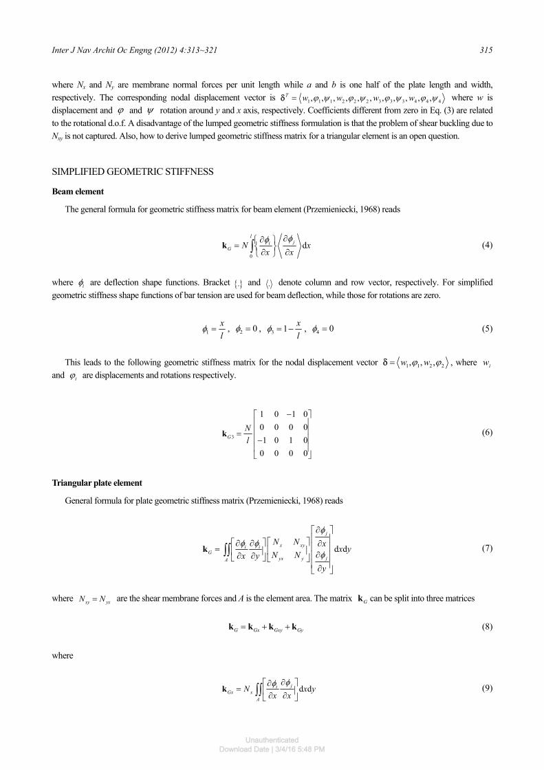
Inter J Nav Archit Oc Engng (2012) 4:313~321 315

where Nx and Ny are membrane normal forces per unit length while a and b is one half of the plate length and width, respectively. The corresponding nodal displacement vector is 1 1 1 2 2 2 3 3 3 4 4 4, , , , , , , , , , ,T w w w wϕ ψ ϕ ψ ϕ ψ ϕ ψ=δ where w is displacement and ϕ and ψ rotation around y and x axis, respectively. Coefficients different from zero in Eq. (3) are related to the rotational d.o.f. A disadvantage of the lumped geometric stiffness formulation is that the problem of shear buckling due to Nxy is not captured. Also, how to derive lumped geometric stiffness matrix for a triangular element is an open question.

SIMPLIFIED GEOMETRIC STIFFNESS

Beam element

The general formula for geometric stiffness matrix for beam element (Przemieniecki, 1968) reads

0

dl

jiG N x

x xφφ ∂∂⎧ ⎫= ⎨ ⎬∂ ∂⎩ ⎭∫k (4)

where iφ are deflection shape functions. Bracket {}. and . denote column and row vector, respectively. For simplified geometric stiffness shape functions of bar tension are used for beam deflection, while those for rotations are zero.

1

xl

φ = , 2 0φ = , 3 1 xl

φ = − , 4 0φ = (5)

This leads to the following geometric stiffness matrix for the nodal displacement vector 1 1 2 2, , ,w wϕ ϕ=δ , where iw and iϕ are displacements and rotations respectively.

3

1 0 1 00 0 0 01 0 1 0

0 0 0 0

GNl

−⎡ ⎤⎢ ⎥⎢ ⎥=⎢ ⎥−⎢ ⎥⎣ ⎦

k (6)

Triangular plate element

General formula for plate geometric stiffness matrix (Przemieniecki, 1968) reads

d d

j

x xyi iG

jyx yA

N N x x yN Nx y

y

φφ φ

φ

∂⎡ ⎤⎢ ⎥⎡ ⎤⎡ ⎤∂ ∂ ∂⎢ ⎥= ⎢ ⎥⎢ ⎥ ∂∂ ∂ ⎢ ⎥⎣ ⎦ ⎣ ⎦⎢ ⎥∂⎣ ⎦

∫∫k

(7)

where xy yxN N= are the shear membrane forces and A is the element area. The matrix Gk can be split into three matrices

G Gx Gxy Gy= + +k k k k (8)

where

d dji

Gx xA

N x yx x

φφ ∂⎡ ⎤∂= ⎢ ⎥∂ ∂⎣ ⎦

∫∫k (9)



d dj ji i

Gxy xyA

N x yx y y x

φ φφ φ∂ ∂⎡ ⎤∂ ∂= +⎢ ⎥∂ ∂ ∂ ∂⎣ ⎦

∫∫k (10)

d dji

Gy yA

N x yy y

φφ ∂⎡ ⎤∂= ⎢ ⎥∂ ∂⎣ ⎦

∫∫k (11)

Shape functions for in-plane displacements of the triangular element (Zienkiewicz, 1971) as shown in Fig. 1 are used as

( )

( )

( )

1 1 23 32

2 2 31 13

3 3 12 21

121

21

2

y x x yA

y x x yA

y x x yA

φ α

φ α

φ α

= + +

= + +

= + +

(12)

where

1 2 3 3 2 2 3 1 1 3 3 1 2 2 1, ,x y x y x y x y x y x yα α α= − = − = − (13)

, , , 1,2,3ij i j ij i jx x x y y y i j= − = − = (14)

( )21 31 31 21

12

A x y x y= − (15)

Fig. 1 Triangular finite element.

The derivatives of the shape functions are constants as follows:

1 123 32

2 231 13

3 312 21

1 1,2 21 1,

2 21 1,

2 2

y xx A y A

y xx A y A

y xx A y A

φ φ

φ φ

φ φ

∂ ∂= =

∂ ∂∂ ∂

= =∂ ∂∂ ∂

= =∂ ∂

(16)



Using Eq. (16), the stiffness matrices (9), (10) and (11) can be derived as follows:

223 23 31 23 12

231 31 12

212

4.

xGx

y y y y yN y y y

ASym y

⎡ ⎤⎢ ⎥= ⎢ ⎥⎢ ⎥⎣ ⎦

k (17)

23 32 23 13 32 31 23 21 32 12

31 13 31 21 13 12

12 21

22

4. 2

xyGxy

y x y x x y y x x yN

y x y x x yA

Sym y x

+ +⎡ ⎤⎢ ⎥= +⎢ ⎥⎢ ⎥⎣ ⎦

k (18)

232 32 13 32 21

213 13 21

221

4.

yGy

x x x x xN

x x xA

Sym x

⎡ ⎤⎢ ⎥= ⎢ ⎥⎢ ⎥⎣ ⎦

k (19)

The above matrices are derived for displacements d.o.f. 1 2 3, ,w w w=δ due to reason of simplicity. Therefore, it is necessary to spread them to the complete 9x9 displacement field, which includes displacement as well as rotations, i.e.

1 1 1 2 2 2 3 3 3, , , , , , , ,T w w wϕ ψ ϕ ψ ϕ ψ=δ . Hence, the matrix elements related to the rotations as well as those related to their coupling with deflection d.o.f. are zero.

Rectangular plate element

A rectangular element in the Cartesian coordinates is shown in Fig. 2. The shape functions for in-plane displacements expressed by non-dimensional coordinates /x aξ = and /y bη = read (Holand and Bell, 1970)

( ) ( )1 1 1

4i i iφ ξ ξ ηη= + + (20)

where iξ and iη are the nodal values as shown in Fig. 3. These shape functions are used for displacement and one finds for their derivatives

( )

( )

1 141 14

ii i

ii i

x a

y b

φ ξ ηη

φ ξ ξ η

∂= +

∂∂

= +∂

(21)

By substituting (21) into (9), (10) and (11) and performing integration over the element area, one finds the matrix elements

1

4 3i jij x

Gx i jN bk

aηη

ξ ξ⎛ ⎞

= +⎜ ⎟⎝ ⎠

(22)

( )4

xyijGxy i j j i

Nk ξη ξ η= + (23)

1

4 3y i jij

Gy i j

N ak

bξ ξ

ηη⎛ ⎞

= +⎜ ⎟⎝ ⎠

(24)



Furthermore, by taking into account the value of the nodal coordinates as shown in Fig. 3, Eqs. (22), (23) and (24) lead to the geometric stiffness matrices

2 2 1 12 1 1

2 26. 2

xGx

N ba

Sym

− −⎡ ⎤⎢ ⎥−⎢ ⎥=⎢ ⎥−⎢ ⎥⎣ ⎦

k (25)

1 0 1 01 0 1

1 02. 1

xyGxy

N

Sym

−⎡ ⎤⎢ ⎥−⎢ ⎥=⎢ ⎥⎢ ⎥−⎣ ⎦

k (26)

2 1 1 22 2 1

2 16. 2

yGy

N ab

Sym

− −⎡ ⎤⎢ ⎥− −⎢ ⎥=⎢ ⎥⎢ ⎥⎣ ⎦

k (27)

Fig. 2 Rectangular finite element in Fig. 3 Rectangular finite element in

Cartesian coordinate system. non-dimensional coordinates.

The above matrices are derived for displacement d.o.f. 1 2 3 4, , ,w w w w=δ , and therefore they have to be spread to the complete displacement field of 12×12 terms, which includes also rotational d.o.f. 1 1 1 2 2 2 3 3 3 4 4 4, , , , , , , , , , ,w w w wϕ ψ ϕ ψ ϕ ψ ϕ ψ=δ , in a similar way as explained in the triangular element.

NUMERICAL EXAMPLES

Beam buckling

Let us consider the stability of simply supported beam of the following particulars: length 40L = m, the cross-section area of 2csA = m2, the moment of inertia of the cross-section is 0.1667I = m4 and the Young's modulus is 112.1 10E = ⋅ Pa.

The analytical formula defining the critical buckling force reads (Timoshenko and Gere, 1961)

2

2crEIN

Lπ

= (28)

that gives 215.7crN = MN. The critical buckling force is also determined by the finite element method for consistent, simplified,



lumped and hybrid geometric stiffness matrix

( )4 2 3

12G G G= +k k k (29)

The beam is divided into 8 and 16 finite elements. The obtained results are listed in Table 1. They converge with increasing the number of finite elements. The consistent geometric stiffness introduces quite small error. The simplified and lumped stiffness overestimate and underestimate the results respectively. Hence, the hybrid stiffness reduces the discrepancy considerably.

Table 1 Beam buckling force Nxcr [MN].

Number of finite elements Analytical Consistent

kG1 Simplified

kG3 Lumped

kG2 Hybrid

kG4 Discrepancies, %

δ1 δ3 δ2 δ4

8 215.7 215.91 218.69 213.09 216.58 0.090 1.370 -1.226 0.408

16 215.7 215.89 216.59 215.21 216.07 0.088 0.412 -0.230 0.171

Plate buckling

The application and evaluation of the simplified geometric stiffness matrix for defining the critical buckling force is illustrated in the case of a simply supported plate. The analytical solution of critical axial load of a rectangular plate, according to Timoshenko and Gere (1961), reads

( )2 3

2 24 ,

12 1xcrD EtN k D

bπ

ν= =

−

(30)

where t is plate thickness and k is factor which depends on the aspect ratio a/b, i.e. plate length and width a and b respectively. For square plate k=1.

A numerical example is performed by the use of finite element method for a square plate of the following dimensions 2a b= = m, and 0.01t = m. The plate is divided into 4×4=16 and 8×8=64 square finite elements, respectively. The conven-

tional stiffness matrix is determined by employing the non-conforming rectangular finite element, (Szilard, 2004). Consistent, simplified, lumped and hybrid geometric stiffness matrix are taken into account. The obtained results are compared with the analytical solution in Table 2. The consistent geometric stiffness matrix gives quite good results, which converge from below. They are very close to those shown in (Holand and Bell, 1970). The results obtained by the simplified and lumped matrices converge from the opposite sides and the solution obtained by the hybrid matrix is very good and close to the one of the consistent matrix. Commercial software NASTRAN used to define the buckling factor k, which are also included in Table 2 and they are the best ones among the numerical solutions, (MSC, 2005).

Table 2 Buckling factor k for simply supported square plate, uniform axial compression Nx, analytical value k=1.

Mesh Consistent kG1

Simplified kG3

LumpedkG2

HybridkG4

NASTRANkG5

Discrepancies, %

δ1 δ3 δ2 δ4 δ5

4×4 0.9449 1.0905 0.7655 0.9452 1.0280 -5.83 8.30 -30.63 -5.79 2.72

8×8 0.9888 1.0213 0.9339 0.9882 1.0003 -1.13 2.09 -7.08 -1.20 0.03

Furthermore, the buckling of the same square plate due to uniformly distributed shear forces is analysed here. The critical

buckling force is determined analytically by the use of the Fourier series (Timoshenko and Gere, 1961), and can be presented in the similar form as Eq. (26), i.e.



2

2xycrDN k

bπ

= (31)

where k=9.4. The finite element results are shown in Table 3. The best results are obtained by the consistent geometric stiffness matrix, which is better than the one obtained by NASTRAN. The simplified matrix produces results of the same order of discrepancies as NASTRAN. A mesh density 4x4 elements gives very large discrepancies for the both formulations.

Table 3 Buckling factor k for simply supported square plate, uniform shear load Nxy, analytical value k=9.4.

Mesh Consistent kG1

Simplified kG3

NASTRAN kG5

Discrepancies, %

δ1 δ3 δ5

4×4 8.3481 15.5617 14.7962 -12.60 39.60 36.47

8×8 8.9280 10.5616 10.1736 -5.29 11.00 7.60

Buckling modes obtained by NASTRAN in the case of axial and shear load, and for the mesh density 4x4 and 8x8 elements

are shown in Figs. 4 and 5, respectively. The higher mesh density soothes the deflection field.

Fig. 4 Buckling modes of simply supported plate for axial load and different mesh sizes.

Fig. 5 Buckling modes of simply supported plate for shear load and different mesh sizes.



CONCLUSIONS

The consistent geometric stiffness matrix is quite complex, and therefore there is a tendency to employ the lumped geo-metric stiffness, determined in analogy with the lumped mass matrix. However, a simplified geometric stiffness matrix, by employing shape functions of in-plane displacements, can be derived, as it is shown for beam and triangular and rectangular finite elements. Due to a lower order of interpolation polynomials, integration of the shape functions is performed analytically and a quite simple geometric stiffness matrix is obtained. The results obtained with the simplified and lumped matrix, converge from the opposite sides, and the hybrid matrix, as an average of these two, can be used in order to increase the accuracy. How-ever, a disadvantage of the lumped geometric stiffness matrix is that shear buckling cannot be captured. Also, the possibility of deriving of a lumped matrix for a triangular element is questionable. The numerical examples of simply supported beam and plate, modelled with rectangular elements, shown that the simplified geometric stiffness matrix can be successfully used in restoring stiffness for the hydroelastic analysis of ship and offshore structures. Due to complexitiy of the structures triangular element will be also used.

ACKNOWLEDGEMENTS

This work was supported by the National Research Foundation of Korea (NRF) grant funded by the Korea Government (MEST) through GCRC-SOP (Grant No. 2011-0030669).

REFERENCES

Bathe, K.J., 1996. Finite element procedures. Prentice Hall. Cook, R.D., Malkus, D.S. and Plesha, M.D., 1989. Concepts and applications of finite element analysis. 3rd ed. John Wiley

& Sons. Holand, I. and Bell, K., 1970. Finite element methods in stress analysis. Tapir Forlag, Trondheim. Huang, L.L. and Riggs, H.R., 2000. The hydrostatic stiffness of flexible floating structure for linear hydroelasticity. Marine

Structures, 13(2), pp.91-106. Kilroy, K., 1997. MSC/NASTRAN, Quick reference guide. The MacNeal-Schwendler Corporation. MSC, 2005. MSC.NASTRAN2005: Installation and operations guide. MSC Software. Przemieniecki, J.S., 1968. Theory of matrix structural analysis. McGraw-Hill. Senjanović, I., Hadžić, N. and Tomić, M., 2011. Investigation of restoring stiffness in the hydroelastic analysis of slender

marine structures. ASME Journal of Offshore Mechanics and Arctic Engineering, 133(3), Paper No. 031107. Senjanović, I., Vladimir, N. and Hadžić, N., 2010. Some aspects of geometric stiffness modelling in the hydroelastic

analysis of ship structures. Transactions of FAMENA, 34(4), pp.1-10. Shah, S.J., 2001. Finite-element geometric stiffness matrix lumping by numerical integration for stability analysis. Tran-

sactions, SMiRT 16. Washington DC, Paper 2057. Szilard, R., 2004. Theories and applications of plate analysis. John Wiley & Sons. Timoshenko, S.P. and Gere, J.M., 1961. Theory of elastic stability. McGraw-Hill. Zienkiewicz, O.C., 1971. The finite element method in engineering science. London: McGraw-Hill.


Documents

A simplified geometric stiffness in stability analysis …repozitorij.fsb.hr/3916/1/ijnaoe-2013-0099.pdf · The finite element method is very efficient tool for structural analysis