Original Article

Journal of Strain Analysis47(1) 18–31� IMechE 2011Reprints and permissions:sagepub.co.uk/journalsPermissions.navDOI: 10.1177/0309324711430023sdj.sagepub.com

A simplified approach for flexuralbehavior of epoxy resin materials

Masoud Yekani Fard, Yingtao Liu and Aditi Chattopadhyay

AbstractA piecewise-linear parametric uniaxial tension and compression stress–strain model with a simplified post-peak responseis developed to obtain the nonlinear load deflection response of epoxy resin materials which are considerably strongerin compression than tension. This model could be used to obtain flexural strength when the complete post-peak beha-vior of the material in tension and compression is not available. The tension and compression stress–strain curves arebilinear for pre-peak response followed by a constant flow stress in tension and a constant yield stress in compression inthe post-peak response. The simulations and experiments reveal the suitability of this model for predicting the three-point bending and four-point bending response. This model gives an upper bound estimate for flexural over-strengthfactor.

KeywordsEpoxy resin, stress–strain relations, moment distribution, curvature, load, deflection, three-point bending (3PB), four-point bending (4PB), nonlinear response

Date received: 26 July 2011; accepted: 26 October 2011

Introduction

Epoxy resins are one of the most common matrix mate-rials in fiber reinforced composites. However, theirmechanical properties and the progressive failure pat-terns present a challenge for researchers investigatingthe integrity of these materials under different loadingconditions. In structural applications, large flexuralloads are considered one of many critical loading casesconsidered in the design of polymer-based compositestructures. Developing a constitutive stress–strain rela-tionship is difficult due to the need for characterizationof mechanical behavior at different loading conditions.To the best of this authors’ knowledge, no analyticalmaterial characterization study exists in the literaturethat relates to the tension, compression, and flexuralbehavior of a single type of epoxy resin material.

Hydrostatic stresses are known to affect the yieldstress and nonlinear response of epoxy resin materials.1

Several three-dimensional viscoelastic and/or viscoplas-tic constitutive models have been proposed for in-planetension and compression material behavior.2–10 Thesemodels have been successful, especially, in fitting quasi-static test results. They have also been able to partiallydescribe the material response at different strain rates.Jordan et al.11 and Lu et al.12 modified the constitutivemodels developed by Boyce et al.5 and Hasan and

Boyce6 to obtain uniaxial compressive stress–strainbehavior of epoxy resins. Bodner and Partom13 utilizeda set of viscoplastic state variable constitutive equationsto represent the inelastic behavior of Rene 95 at 650 �C.Zhang and Moore14 and Gilat et al.15 used the Bodner–Partom theory13 to obtain the inelastic uniaxial responseof polymers. Li and Pan,16 Chang and Pan,17 and Hsuet al.18 developed a model for polymeric materials bymodifying the pressure-dependent Drucker–Prager yieldcriteria, originally introduced to deal with the plasticdeformation of soils.19 A piecewise-linear tension andcompression stress–strain relationship was used to studythe mechanical behavior of high-performance fiber-rein-forced cement composites by Naaman and Reinhardt.20

The piecewise-linear approach was used to study flex-ural behavior of cement-based composite materials.21–23

Three-point bending (3PB) tests were used to study thedifferent environmental and aging effects on mechanical

Department of Mechanical and Aerospace Engineering, Arizona State

University, USA

Corresponding author:

M Yekani Fard, Department of Mechanical and Aerospace Engineering,

School of Engineering of Matter, Transport and Energy, Arizona State

University, Arizona, Tempe 85287, USA.

Email: masoud.yekanifard@asu.edu

properties of different types of fiber posts.24 Digitalspeckle photogrammetry technique was used to studythe effect of defects on flexural behavior of sandwichcomposite structures by Fergusson et al.25 Yekani Fardet al.26,27 studied the nonlinear mechanical behavior ofEpon E 863 using the digital image correlation (DIC)system. Hobbiebrunken et al.,28 Bazant and Chen,29

Odom and Adams,30 and Goodier31 studied the depen-dency of the failure and strength on the size effect, stressstate, and volume of the body subjected to stress inepoxy resin polymers. Giannotti et al.32 and Vallo33

used the statistical Weibull analysis approach and esti-mated the mean flexural strength to be 40% higher thanthe tensile strength for a Weibull modulus greater than14. Yekani Fard et al.34,35 used an analytical approachto evaluate the flexural over-strength factor in epoxyresin E 863. They observed that the flexural strength in3PB beams with groove was at least 14% higher thanthe tensile peak stress at low strain rates. Flexural over-strength factor is the ratio of the flexural strength (peakstress) to the ultimate tensile strength (UTS). Figure 1shows the concept of the flexural over-strength factordue to the stress gradient effect along a potential frac-ture path. Using flexural over-strength factor, the nom-inal uniaxial material capacities are increased.

Jordan et al.,11 Yekani Fard et al.,27 G’Sell andSouahi,36 Boyce and Arruda,37 Buckley and Harding,38

Shah Khan et al.,39 Littell et al.,40 Chen et al.41 andGerlach et al.42 studied the tension and compressionstress–strain curves in different polymers at differentstrain rates and environmental conditions. Epoxy resinmaterials exhibit the following distinct behavior in thetension and compression stress–strain behavior: linearlyelastic, nonlinearly ascending pre-peak response, yield-like (peak) behavior, strain softening, and plastic flowor strain stiffening at high strain in some cases. YekaniFard et al.27 showed that many common strain anddeformation techniques such as strain gages, extens-ometers and actuators result either in no information ofpost-peak behavior or in an average strain over a speci-men in the post-peak response. Averaging the strain

over a specimen that is deforming non-homogeneously,especially in the plastic range, does not capture the postpeak response accurately. Therefore, sufficient data ofthe post-peak mechanical behavior in tension and com-pression are not available.

In this study, a piecewise-linear tension and com-pression stress–strain model with constant plastic flowstress in tension and constant yield stress in compres-sion in the post-peak response is used to obtain theflexural load deflection response in epoxy resin E 863,which is considerably stronger in compression than intension. An inverse analysis technique is used to obtainthe modified peak uniaxial strengths for the constantplastic stress model considering the flexural over-strength factor. The purpose of this study is two-fold:(i) to introduce a simplified modeling technique toobtain flexural strength of epoxy resins when sufficientdata of post-peak behavior in tension and compressionare not available; (ii) to compare the flexural over-strength factor for 3PB with groove and four-pointbending (4PB) beams.

Constant plastic stress for tension and compression

To study the flexural response in E 863, Yekani Fardet al.34,35 used a piecewise-linear tension and compres-sion stress and strain model with strain softening, curvefitted to the experimentally obtained, uniaxial stress–strain curves, as shown in Figure 2. While the compres-sive and tensile moduli are approximately equal for E863, the stress of the first point showing deviation fromlinearity in the stress–strain curve and the peak stressin tension are lower than those in compression. This isthe main reason that E 863 does not experience com-pression plastic flow in bending and their stress–strain

Figure 2. Experiment and strain softening tension and com-pression model at 493 mstr/sec.Figure 1. Stress gradient effect on maximum flexural strength.

Yekani Fard et al. 19

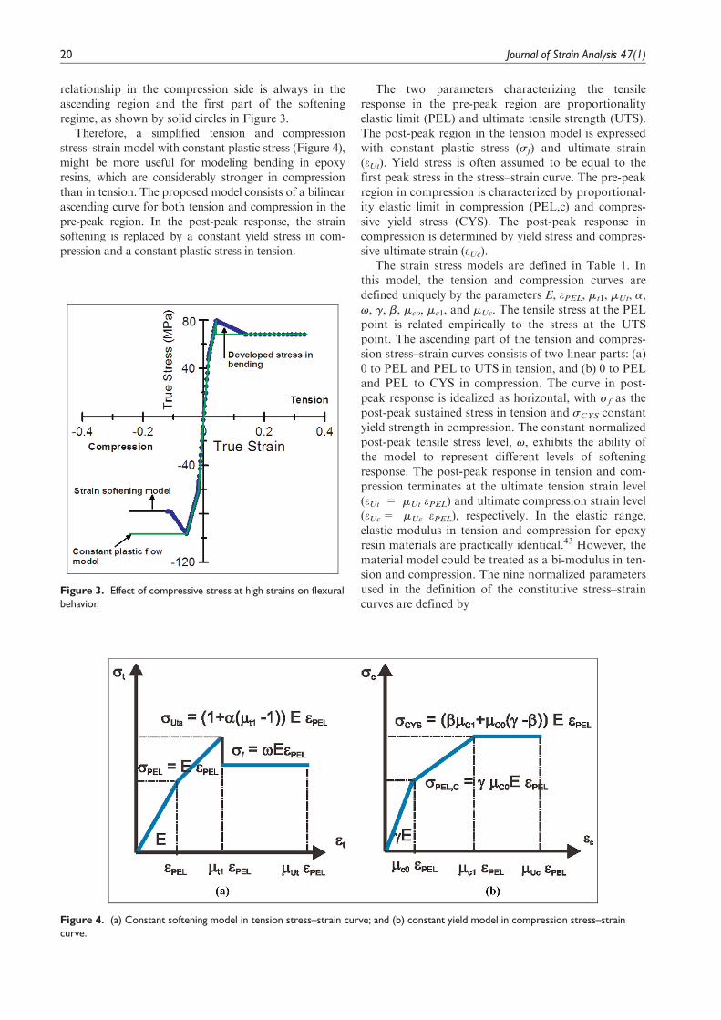
relationship in the compression side is always in theascending region and the first part of the softeningregime, as shown by solid circles in Figure 3.

Therefore, a simplified tension and compressionstress–strain model with constant plastic stress (Figure 4),might be more useful for modeling bending in epoxyresins, which are considerably stronger in compressionthan in tension. The proposed model consists of a bilinearascending curve for both tension and compression in thepre-peak region. In the post-peak response, the strainsoftening is replaced by a constant yield stress in com-pression and a constant plastic stress in tension.

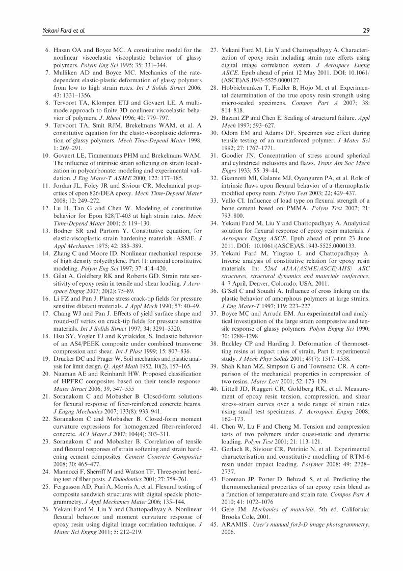
The two parameters characterizing the tensileresponse in the pre-peak region are proportionalityelastic limit (PEL) and ultimate tensile strength (UTS).The post-peak region in the tension model is expressedwith constant plastic stress (sf) and ultimate strain(eUt). Yield stress is often assumed to be equal to thefirst peak stress in the stress–strain curve. The pre-peakregion in compression is characterized by proportional-ity elastic limit in compression (PEL,c) and compres-sive yield stress (CYS). The post-peak response incompression is determined by yield stress and compres-sive ultimate strain (eUc).

The strain stress models are defined in Table 1. Inthis model, the tension and compression curves aredefined uniquely by the parameters E, ePEL, mt1, mUt, a,v, g, b, mco, mc1, and mUc. The tensile stress at the PELpoint is related empirically to the stress at the UTSpoint. The ascending part of the tension and compres-sion stress–strain curves consists of two linear parts: (a)0 to PEL and PEL to UTS in tension, and (b) 0 to PELand PEL to CYS in compression. The curve in post-peak response is idealized as horizontal, with sf as thepost-peak sustained stress in tension and sCYS constantyield strength in compression. The constant normalizedpost-peak tensile stress level, v, exhibits the ability ofthe model to represent different levels of softeningresponse. The post-peak response in tension and com-pression terminates at the ultimate tension strain level(eUt = mUt ePEL) and ultimate compression strain level(eUc= mUc ePEL), respectively. In the elastic range,elastic modulus in tension and compression for epoxyresin materials are practically identical.43 However, thematerial model could be treated as a bi-modulus in ten-sion and compression. The nine normalized parametersused in the definition of the constitutive stress–straincurves are defined by

Figure 4. (a) Constant softening model in tension stress–strain curve; and (b) constant yield model in compression stress–straincurve.

Figure 3. Effect of compressive stress at high strains on flexuralbehavior.

20 Journal of Strain Analysis 47(1)

mc0 =ePEL, cePEL

, mc1 =eCYSePEL

, mUc =eUc

ePEL

mt1 =eUts

ePEL, mUt=

eUt

ePELð1Þ

g =Ec

E, b=

EPEL, c

E, a=

EPEL, t

Eð2Þ

v=sf

sPELð3Þ

where mco, mc1, mUc are normalized strain at the propor-tionality elastic limit point in compression, normalizedstrain at the CYS point, and normalized compressivestrain at failure point, respectively. mt1, mUt are normal-ized strain at UTS point and normalized tensile strainat the failure point. Stiffness parameters a, g, and b arenormalized stiffness at post PEL in tension, elastic stiff-ness in compression, and normalized post-PEL stiffness

in compression. v is the normalized constant tensilesoftening stress.

Moment curvature

Figure 4 shows that there are three distinct regions onstress–strain curve for each tension and compressionstress–strain relationship; therefore, there would be ninedifferent cases of stress distribution across any arbitrarycross section, as shown in Figures 5 to 7. Since epoxyresin materials have higher mechanical strengths incompression than in tension, some cases of stress distri-bution are unlikely to occur for epoxy resin materials.However, an algorithm has been developed to accountfor all possible cases, so that any type of material exhi-biting uniaxial tension and compression stress–strain asshown in Figure 4, could be modeled. Linear straincompatibility has been assumed in all these cases. Loadis applied from 0 to failure by imposing a normalizedcompressive strain (l) at top fiber. The area under thestress curves of each tension and compression subzonerepresents the internal longitudinal normal force. Thetension and compression forces normalized to tensionforce at the PEL point (bhEePEL) are summarized inTable 2. The internal normal forces at each step in timeare balanced with the external applied moment.

Stress across a section develops from 0 to inelasticnonlinear in both tension and compression in case nine,shown in Figure 8, as the load is applied incrementally

Figure 5. (a) Rectangular cross section; (b) case1: linear in compression and tension; (c) case 2: elastic in compression and post PELin tension; and (d) case 3: post PEL in compression and elastic in tension.

Table 1. Definition of compression and tension stresses.

Stress Definition Domain of strain

st(et) Eet 0 < et < ePEL

E(ePEL + a (et–ePEL)) ePEL \ et < mt1 ePEL

v E ePEL mt1 ePEL \ et < mUt ePEL

0 mUt ePEL \ et

sc(ec) g E ec 0 < ec < mc0ePEL

E (g mc0 ePEL + b (ec–mc0 ePEL)) mc0 ePEL \ ec < mc1 ePEL

E ePEL (bmc1 + mc0 (g-b)) mc1 ePEL \ ec < mUc ePEL

0 mUc ePEL \ ec

Yekani Fard et al. 21

at the top fiber. Stress may not develop up until stagesix (Figure 8), considering the value of tension andcompression parameters, but stress develops at least tostage four, where compressive failure is possible if lmax

= mUc in case 6, or tensile failure may happen whenlmax = W in case four.

Stress evolution through the stages, shown inFigure 8, depends on the characteristic points (R to Z),which are functions of the material parameters, and thecontrolling value lmax. Transition points, defined bythe parameter tpij between different stages in Figure 8,are described as follows

tp12 =Min(mco, R)

tp23 =Min(mco, T) or Min (mc1, S)

tp34 =Min(mUc, U) or Min (mc1, V) or Min (mco,W)

tp45 =Min(mUc, X) or Min (mc1, Y)

tp56 =Min(mUc, Z)

ð4Þ

where indices i and j refer to origin and destinationstages, respectively. Characteristic points R to Z arecalculated as functions of material parameters to satisfythe following relation at each load step

Figure 6. (a) Case 4: elastic in compression and constant softening in tension; (b) case 5: post PEL in compression and tension; (c)case 6: constant yield in compression and elastic in tension; and (d) case 7: post PEL in compression and constant softening in tension.

Figure 7. (a) Case 8: constant yield in compression and post PEL in tension; and (b) case 9: constant yield in compression and con-stant softening in tension.

22 Journal of Strain Analysis 47(1)

et < V ePEL ð5Þ

where et is the tensile strain at the bottom fiber and V isone of the following {1, mt1, mUt}. et is expressed as a lin-ear function of the applied compressive strain at the topfiber (ec), which is equal to l ePEL, and k is the depth ofthe neutral axis and is a function of material parameters

et =1� k

kec ð6Þ

As the applied load lePEL is incrementally imposed,the strain and stress distribution is determined and theinternal tension and compression forces are computed.The location of the neutral axis k throughout the

Figure 8. Stress development at different stages of flexural loading.

Table 2. Tension and compression forces for each subzone in all cases.

Case Ft1 or Fc1

bhE ePEL

Ft2 or Fc2

bh E ePEL

Ft3 or Fc3

bh E ePEL

1,3,6 tension lk

2� l +

l

2k

— —

2,5,8 tension k

2ll + 1ð Þpk

2l+�2al2 � 2al + 2l

2l

+al

2k, p = � 2 + al + a

—

4,7,9 tension k

2l(2 + amt1 � a)(mt1 � 1)k

2l

�v l + mt1ð Þkl

+ v

1,2,4 compression glk

23,5,7 compression gm2

c0k

2l

q l� mc0ð Þk2l

q = 2gmc0 + b l� mc0ð Þ6,8,9 compression gm2

c0k

2l

r mc1 � mc0ð Þk2l

r = 2gmc0 + b mc1 � mc0ð Þ

s l� mc1ð Þkl

s = gmc0 + b mc1 � mc0ð Þ

Yekani Fard et al. 23

loading is obtained by imposing the equilibrium condi-tion at each case for each step of load

X3i=1

Fti �X3j=1

Fcj = 0 ) km a,b, g,v,mt1,mc0,mc1,lð Þ

ð7Þ

where Fci and Fti for (i = 1, 2, 3) are tension and com-pression forces calculated from the stress diagrams.Tension and compression forces for case nine are pre-sented in Appendix 2. The equilibrium governing equa-tion in some cases results in more than one solution fork, but the valid value of k is between 0 and 1. Figure 9shows the negligible unbalanced normalized internalforce using the correct expressions for k throughoutloading. For a beam with a cross section of 4 3 7mm2,E = 3049MPa, and ePEL= 0.0162, the amount ofunbalanced internal force is 1.4 3 10212N, which isnegligible. The expressions for k are presented inAppendix 3. By substituting the expressions for k inequation (5), the characteristic points R to Z as func-tions of material parameters are calculated.

As an example, the steps to obtain the normalizedmoment and curvature expressions for case nine inFigure 7 are explained in detail in Appendix 2. Thegeneral definitions for normalized moment and curva-ture are shown in equations (8) through (10)

M l, g,b,a,mc0,mc1,mt1,mUt,mUc,vð Þ =MPELM

0 l, g,b,a,mc0,mc1,mt1,mUt,mUc,vð Þ ð8Þ

u l, g,b,a,mc0,mc1,mt1,mUt,mUc,vð Þ =uPEL u0 l, g,b,a,mc0,mc1,mt1,mUt,mUc,vð Þ ð9Þ

u0i l, g,b,a,mc0,mc1,mt1,mUt,mUc,vð Þ =l

2ki, i=1, 2, 3, . . . , 9 ð10Þ

where MPEL and uPEL are moment and curvature atthe elastic limit, and are defined as follows.

MPEL=bh2EePEL

6, uPEL =

2ePELh

ð11Þ

The expressions for the normalized moment are sum-marized in Appendix 3. If there is no intrinsic flaw in amaterial, Mu could approach MN for very large l val-ues. In this ideal situation, the normalized moment atvery large l values, M#N, is computed by substitutingl=N in the expression for k in case nine, and by sub-stituting l=N and kN in the normalized momentexpression. Equations (12) through (14) present the val-ues of the neutral axis depth, normalized moment, andcurvature for very large l values

k‘ =v

v+ gmc0 � bmc0 +bmc1

ð12Þ

M0‘ =3v gmc0 � bmc0 +bmc1ð Þv+ gmc0 � bmc0 +bmc1

ð13Þ

u0‘ = ‘ ð14Þ

The neutral axis depth and normalized moment arefunctions of material parameters in compression (g, b,mc0, mc1) and constant normalized tensile plastic stress(v). Expression gmc0 + b (mc12 mc0) is the definitionof normalized sCYS. For flawless epoxy resin materialswith very low tensile plastic stress, the normalizedmoment is almost three times the normalized tensileplastic stress. The normalized neutral axis depth ratioand moment for an elastic perfectly plastic material aslogically expected are 0.5 and 1.5, respectively.44 For aset of parameters, g, b, mc0, mc1, the critical value of v,which results in a flexural capacity at infinity (failure)greater than the flexural capacity at the tensile PELpoint, can be found. By equating the normalizedmoment for large top compressive strain to one(M#N=1), the critical value of normalized tensile plas-tic stress, vcritical, is

vcritical =gmc0 � bmc0 +bmc1

3 gmc0 � bmc0 +bmc1ð Þ � 1ð15Þ

The required parameters for Epon E 86240 and E86327 have been defined through curve fitting to the ten-sion and compression stress–strain curves. Calculationsshow the vcritical for E 862 and E 863 as 0.39 and 0.4,respectively (almost 25% of the ultimate tensile strength).

Parametric study

Yekani Fard et al.34,35 studied the effect of differentparts of strain softening tension and compressionstress–strain models on the flexural response. A set ofparametric studies based on the proposed constant plas-tic stress model were performed to determine the impor-tant parameters for flexural load-carrying capacity.Tension and compression stress–strain curves of EponE 86240 was chosen as the base parameters: E=2069

Figure 9. Negligible unbalanced internal force throughoutloading.

24 Journal of Strain Analysis 47(1)

MPa, Ec=2457 MPa, ePEL=0.0205, eUts=0.076,eUt=0.24, ePEL,c=0.019, eCYS=0.092, eUc=0.35,sUts=70MPa, sf=60.5 MPa, sCYS=93MPa.

Figures 10(a) and (b) depict the effect of ultimatetensile stress with constant PEL slope and constant ten-sile softening stress on the moment curvature and neu-tral axis location. Figure 10(b) reveals that an increasein mt1 considerably increases flexural strength.However, the amount of moment at failure is notaffected as much as the flexural strength, since for mt1

. 6, the moment at infinity is less than the flexuralstrength. The effectiveness of ultimate tensile strengthon moment-carrying capacity was also observed usingthe softening model developed by Yekani Fard et al.34

It is possible to look at the variation of mt1 as the varia-tion of sCYS to sUTS ratio defined as

gmc0 +b mc1 � mc0ð Þ1+ a mt1 � 1ð Þ

By substituting g =1.19, b=0.3, a=0.24, mc0=0.93,mc1=4.49, it is clear that changes in mt1 from 2.75 to 8will change the sCYS to sUTS ratio from 1.53 to 0.81.

The effects of strain at constant ultimate tensilestress on the flexural behavior are presented in Figure11(a) and (b). Figure 11 reveals that changes in para-meters a and mt1 slightly affect the moment butextremely affect the position of the neutral axis for awide range of normalized top compressive strainsbetween one and four, which in turn will change thestress distribution across the cross section between elas-tic and post-peak range. For a resin material withoutany intrinsic flaws, the analysis indicates that tension isthe governing failure mechanism in all cases, whilecompression strain just exceeds the yield point.

Algorithm for load deflection response

An experimental investigation of the tension, compres-sion, and 3PB flexural behavior of Epon E 863 was pre-sented by Yekani Fard et al.26,27 It was shown thatEpon E 863 demonstrates strain softening behavior intension and compression, and higher yield and soften-ing stresses in compression than ultimate tensile andsoftening stresses in tension. Based on these observa-tions, a strain softening tension and compression modelwas used to obtain the nonlinear moment curvatureresponse for Epon E 863.34,35 It was observed that thestrain softening model accurately captures the momentcurvature response in pre-peak and post-peak portions.After curve fitting the constant softening stress modelto the experimental tension and compression stress–strain curves, the normalized moment curvatureresponse is obtained. Figure 12 compares the normal-ized moment curvature diagram from the proposedconstant plastic flow model and the strain softeningmodel34,35 at 493mstr/sec. The constant flow stressmodel differs slightly from the strain softening model inthe pre-peak portion of the response. However, it can-not predict the softening behavior in the moment cur-vature response. This is mainly due to the perfectlyplastic model in compression. The proposed constantplastic flow model shows the same moment carryingcapacity for E 863 as the softening model does, but atdifferent curvatures and only if there is no intrinsic flawin the material. The load deflection response is obtainedusing the nonlinear moment curvature response andestablishing static equilibrium. In displacement control,the normalized top compressive strain is incrementallyimposed from 0 to failure, in order to generate a stressdistribution profile in a given cross section.

Figure 10. Effect of ultimate tensile strength with constant post PEL slope on flexural behavior.

Yekani Fard et al. 25

For resins such as E 862 and E 863, since the com-pressive strength is greater than the tensile strength, theshape of the moment curvature diagram greatly dependson the tensile stress–strain model, as observed in theparametric study. The constant flow curve in Figure 12shows a typical nonlinear moment curvature diagram,based on the constant plastic flow stress model forepoxy resins, consisting of a linear elastic part followedby an ascending curve with reduced stiffness.

The first deviation from linearity in a moment curva-ture or load deflection curve is called limit of propor-tionality (LOP). The specimen is loaded from 0 to PLOP

in the linear portion of the moment curvature diagramfrom 0 to MLOP. The curvature for the linear elasticportion is determined directly from the moment curva-ture diagram. Beyond the LOP, the curvature isobtained from the nonlinear portion of the momentcurvature diagram. Static equilibrium is used to obtaina series of load steps in 3PB or 4PB setups from themoment curvature diagram. The main steps to calculateload deflection response are summarized as follows.

1. Calculate transition points to determine the possi-ble cases of stress distribution based on materialproperties for a piecewise-linear model.

2. Impose load incrementally by increasing the nor-malized compressive strain in top fiber to obtainthe nonlinear moment curvature response usingclosed-form expressions for moment and curvaturerelevant to the cases in step one.

3. Calculate applied load vector (P=2M/S where Sis the span and the distance between a support andadjacent load for the 3PB and 4PB, respectively).

4. Calculate moment diagram along the structure forany load in step three.

5. Determine curvature diagram for any load in stepthree along the structure using moment curvaturerelationship.

6. Calculate amount of deflection using one of themethods for statically determinate structures (e.g.virtual work method or moment area method).

7. Repeat steps three to six for each load.

Experiments

Tension, compression, 3PB bending beams with groove,and 4PB beam tests were conducted on epoxy resinEpon E 863 with a hardener EPI-CURE 3290 using a

Figure 11. Effect of strain at ultimate tensile stress on the flexural behavior.

Figure 12. Normalized moment curvature diagram from theproposed constant flow model and softening model. LOP: limitof proportionality.

26 Journal of Strain Analysis 47(1)

100/27 weight ratio at room temperature and at lowloading speeds. The DIC system, ARAMIS 4M,45 wasused to study the strain fields. Dog bone samples with agage length of 14mm and a rectangular cross-section of3.183 3.43mm2 were selected to conduct the mono-tonic tensile tests. Small cubic samples (43 43 4mm3),right square-sided prisms with length of 8mm and sideof 3.5mm and cylinders with a length of 10mm anddiameter of 4mm were tested under monotonic com-pression. Small beams with the width of 4mm, thick-ness of 10mm, and length of 60mm (50mm span) wereselected to conduct 3PB and 4PB tests. A groove (radiusof approximately 3.5mm) was cut in the middle of thebeam for 3PB tests. The middle span in the 4PB testswas 25mm. Details of the experiments were explainedin the authors’ other publications.26,27

Simulation of 3PB and 4PB flexural load deflectionresponse

The strain softening model for both tension and compres-sion, developed by Yekani Fard et al.,34 demonstratedthat the uniaxial tension and compression stress–straincurves underestimate the load deflection response due toa difference between the stress distribution profile in theuniaxial and bending tests. Figure 13 illustrates the repre-sentative experimental tension and compression truestress–strain curves at 493mstr/sec. As stated before,Epon E 863 has a strain softening behavior in tensionand compression. The constant plastic stress model wasbuilt through curve fitting and is shown as a solid line inFigure 13. The two main parameters and nine non-dimensional parameters for the model at 493mstr/sec are:E=3049 MPa, ePEL=0.0162, mc0=1.148, mc1=3.52,

mc2=6.79, mUc=15.70, mc1=2.55, mUt=20.98,g =1.09, a=0.395, b=0.298, and v=1.369.Simulations were conducted to study the flexural loaddeflection response of Epon E 863 and to evaluate thesuitability of the constant flow stress model and theeffects of out-of-plane loading. Figure 14 shows the 3PBand 4PB load deflection curve compared with the simula-tion results. This figure illustrates that the direct use oftension and compression stress–strain model follows theflexural response in the pre-peak portion and underesti-mates the flexural strength as it is logically expected.However, the simulated load deflection curve obtainedfrom the constant flow stress model is not able to capturethe deflection softening behavior. The main reason forthe underestimation of the flexural strength is that, in ten-sion and compression, the entire volume of the sample issubjected to the same load as shown in Figure 1 and hasthe same probability of failure. Therefore, the probabilityof crack nucleation, propagation, and failure develop-ment in tension and compression samples is higher thanin bending samples. Results of the parametric study showthat flexural load-carrying capacity can be improved byincreasing the ultimate tensile and compressive levelsthrough an over-strength flexural factor (parameter C1)and by further adjustments to the other parameters. Theparameter C1 was calculated to modify the uniaxial strainsoftening tension and compression stress–strain model forflexural simulation.34 Figure 14 shows underestimation inthe prediction of load carrying capacity for 3PB and 4PBusing constant flow stress model. In order to quantifyparameter C1, an inverse analysis technique has been usedto obtain the stress–strain model.

An inverse analysis of the 3PB and 4PB load deflec-tion response showed that the value of C1 for Epon E

Figure 13. (a) Constant flow tension model and stress–strain curve from dogbone samples; and (b) constant yield compressionmodel and stress–strain curve from cubic samples.

Yekani Fard et al. 27

863 was around 1.30 and 1.55, respectively. The reasonfor the higher factor in 4PB than 3PB is that in 3PB,with a groove or notch at the center, the beam is forcedto fracture at the location of the groove or notchcaused by stress concentration. However, the beam’scenter may not be the weakest point in the beam, sothe groove and notch may influence the actual strengthof the material. The results from the analyticalapproach could be compared with the results fromWeibull analysis approach32,33 which estimated themean flexural strength to be 40% higher than the ten-sile strength. More studies at different strain rates andon different epoxy resin materials need to be performedbefore an average flexural over-strength factor can berecommended.

Conclusions

A piecewise-linear stress–strain relation with simplifiedpost-peak response in tension and compression for flex-ural simulation of epoxy resin materials has been pro-posed. This model consists of a bilinear ascendingcurve in the pre-peak portion and constant flow stressin the post-peak tension and compression. The materialmodel is described using two intrinsic material para-meters (tensile modulus of elasticity and tensile strainat the PEL point), in addition to nine non-dimensionalparameters for tension and compression. It was con-cluded that compression stress–strain parameters haveless effect on flexural behavior than tension parameters,as long as material is stronger in compression than intension. Epoxy resin materials with a considerableamount of post-peak tensile strength have a momentcapacity of approximately 2.4 times the elastic moment.Simulation of the load deflection response of epoxy

resins in 3PB and 4PB test revealed the effect of stressgradient on material behavior. Results indicate thatdirect use of tension and compression data underesti-mates the flexural strength. The prediction of flexuralload carrying capacity can be improved by applying ascaling factor (C1) to uniaxial tension and compressionstrength. However, the value of C1 is higher for 4PBthan 3PB due to the effect of stress concentration at thelocation of groove in the 3PB beam.

Funding

This project was supported by the Governor’s Office ofEconomic Recovery and Science Foundation Arizona,Vice President for Research, Dr Gary Greenburg,Agreement Number: SRG 0443-10.

Acknowledgements

The authors would also like to acknowledge HoneywellAerospace for providing equal cost share in this project.

References

1. Ward IM and Sweeney J. Mechanical properties of solid

polymers. Chichester: Wiley, 2004.

2. Buckley CP and Jones DC. Glass-rubber constitutive

model for amorphous polymers near the glass transition.

Polymer 1995; 36: 3301–3312.3. Buckley CP and Dooling PJ. Deformation of thermoset-

ting resins at impact rates of strain, part 2. J Mech Phys

Solids 2004; 52(10); 2355–2377.4. Boyce MC, Parks DM and Argon AS. Plastic flow in

oriented glassy polymers. Int J Plasticity 1989; 5: 593–615.5. Boyce MC, Arruda EM and Jayachandran R. The large

strain compression, tension, and simple shear of polycar-

bonate. Polym Eng Sci 1994; 34: 716–725.

Figure 14. Experiment and simulation of flexural 3PB and 4PB load deflection curve.

28 Journal of Strain Analysis 47(1)

6. Hasan OA and Boyce MC. A constitutive model for the

nonlinear viscoelastic viscoplastic behavior of glassy

polymers. Polym Eng Sci 1995; 35: 331–344.7. Mulliken AD and Boyce MC. Mechanics of the rate-

dependent elastic-plastic deformation of glassy polymers

from low to high strain rates. Int J Solids Struct 2006;

43: 1331–1356.8. Tervoort TA, Klompen ETJ and Govaert LE. A multi-

mode approach to finite 3D nonlinear viscoelastic beha-

vior of polymers. J. Rheol 1996; 40: 779–797.9. Tervoort TA, Smit RJM, Brekelmans WAM, et al. A

constitutive equation for the elasto-viscoplastic deforma-

tion of glassy polymers. Mech Time-Depend Mater 1998;

1: 269–291.10. Govaert LE, Timmermans PHM and Brekelmans WAM.

The influence of intrinsic strain softening on strain locali-

zation in polycarbonate: modeling and experimental vali-

dation. J Eng Mater-T ASME 2000; 122: 177–185.11. Jordan JL, Foley JR and Siviour CR. Mechanical prop-

erties of epon 826/DEA epoxy.Mech Time-Depend Mater

2008; 12: 249–272.12. Lu H, Tan G and Chen W. Modeling of constitutive

behavior for Epon 828/T-403 at high strain rates. Mech

Time-Depend Mater 2001; 5: 119–130.13. Bodner SR and Partom Y. Constitutive equation, for

elastic-viscoplastic strain hardening materials. ASME. J

Appl Mechanics 1975; 42: 385–389.14. Zhang C and Moore ID. Nonlinear mechanical response

of high density polyethylene. Part II: uniaxial constitutive

modeling. Polym Eng Sci 1997; 37: 414–420.15. Gilat A, Goldberg RK and Roberts GD. Strain rate sen-

sitivity of epoxy resin in tensile and shear loading. J Aero-

space Engng 2007; 20(2): 75–89.16. Li FZ and Pan J. Plane stress crack-tip fields for pressure

sensitive dilatant materials. J Appl Mech 1990; 57: 40–49.17. Chang WJ and Pan J. Effects of yield surface shape and

round-off vertex on crack-tip fields for pressure sensitive

materials. Int J Solids Struct 1997; 34; 3291–3320.18. Hsu SY, Vogler TJ and Kyriakides, S. Inelastic behavior

of an AS4/PEEK composite under combined transverse

compression and shear. Int J Plast 1999; 15: 807–836.19. Drucker DC and Prager W. Soil mechanics and plastic anal-

ysis for limit design.Q. Appl Math 1952, 10(2), 157–165.20. Naaman AE and Reinhardt HW. Proposed classification

of HPFRC composites based on their tensile response.

Mater Struct 2006, 39, 547–55521. Soranakom C and Mobasher B. Closed-form solutions

for flexural response of fiber-reinforced concrete beams.

J Engng Mechanics 2007; 133(8): 933–941.22. Soranakom C and Mobasher B. Closed-form moment

curvature expressions for homogenized fiber-reinforced

concrete. ACI Mater J 2007; 104(4): 303–311.23. Soranakom C and Mobasher B. Correlation of tensile

and flexural responses of strain softening and strain hard-

ening cement composites. Cement Concrete Composites

2008; 30: 465–477.24. Mannocci F, Sherriff M andWatson TF. Three-point bend-

ing test of fiber posts. J Endodontics 2001; 27: 758–761.

25. Fergusson AD, Puri A, Morris A, et al. Flexural testing of

composite sandwich structures with digital speckle photo-

grammetry. J Appl Mechanics Mater 2006; 135–144.26. Yekani Fard M, Liu Y and Chattopadhyay A. Nonlinear

flexural behavior and moment curvature response of

epoxy resin using digital image correlation technique. J

Mater Sci Engng 2011; 5: 212–219.

27. Yekani Fard M, Liu Y and Chattopadhyay A. Characteri-

zation of epoxy resin including strain rate effects using

digital image correlation system. J Aerospace Engng

ASCE. Epub ahead of print 12 May 2011. DOI: 10.1061/

(ASCE)AS.1943-5525.0000127.28. Hobbiebrunken T, Fiedler B, Hojo M, et al. Experimen-

tal determination of the true epoxy resin strength using

micro-scaled specimens. Compos Part A 2007; 38:

814–818.29. Bazant ZP and Chen E. Scaling of structural failure. Appl

Mech 1997; 593–627.30. Odom EM and Adams DF. Specimen size effect during

tensile testing of an unreinforced polymer. J Mater Sci

1992; 27: 1767–1771.31. Goodier JN. Concentration of stress around spherical

and cylindrical inclusions and flaws. Trans Am Soc Mech

Engrs 1933; 55: 39–44.32. Giannotti MI, Galante MJ, Oyanguren PA, et al. Role of

intrinsic flaws upon flexural behavior of a thermoplastic

modified epoxy resin. Polym Test 2003; 22; 429–437.33. Vallo CI. Influence of load type on flexural strength of a

bone cement based on PMMA. Polym Test 2002; 21:

793–800.34. Yekani Fard M, Liu Y and Chattopadhyay A. Analytical

solution for flexural response of epoxy resin materials. J

Aerospace Engng ASCE. Epub ahead of print 23 June

2011. DOI: 10.1061/(ASCE)AS.1943-5525.0000133.35. Yekani Fard M, Yingtao L and Chattopadhyay A.

Inverse analysis of constitutive relation for epoxy resin

materials. In: 52nd AIAA/ASME/ASCE/AHS/ ASC

structures, structural dynamics and materials conference,

4–7 April, Denver, Colorado, USA, 2011.36. G’Sell C and Souahi A. Influence of cross linking on the

plastic behavior of amorphous polymers at large strains.

J Eng Mater-T 1997; 119: 223–227.37. Boyce MC and Arruda EM. An experimental and analy-

tical investigation of the large strain compressive and ten-

sile response of glassy polymers. Polym Engng Sci 1990;

30: 1288–129838. Buckley CP and Harding J. Deformation of thermoset-

ting resins at impact rates of strain, Part I: experimental

study. J Mech Phys Solids 2001; 49(7): 1517–1538.39. Shah Khan MZ, Simpson G and Townsend CR. A com-

parison of the mechanical properties in compression of

two resins. Mater Lett 2001; 52: 173–179.40. Littell JD, Ruggeri CR, Goldberg RK, et al. Measure-

ment of epoxy resin tension, compression, and shear

stress–strain curves over a wide range of strain rates

using small test specimens. J. Aerospace Engng 2008;

162–173.41. Chen W, Lu F and Cheng M. Tension and compression

tests of two polymers under quasi-static and dynamic

loading. Polym Test 2001; 21: 113–121.42. Gerlach R, Siviour CR, Petrinic N, et al. Experimental

characterisation and constitutive modelling of RTM-6

resin under impact loading. Polymer 2008: 49: 2728–

2737.43. Foreman JP, Porter D, Behzadi S, et al. Predicting the

thermomechanical properties of an epoxy resin blend as

a function of temperature and strain rate. Compos Part A

2010; 41: 1072–107644. Gere JM. Mechanics of materials. 5th ed. California:

Brooks Cole, 2001.

45. ARAMIS . User’s manual for3-D image photogrammetry,

2006.

Yekani Fard et al. 29

Appendix 1

Notation

b beam widthE modulus of elasticity in tension (if g 6¼ 1)

or modulus of elasticity (if g =1)Ec (g) modulus of elasticity in compression if

g 6¼ 1 (normalized term respect to E)EPEL,c(b)

stiffness at the post proportionality limitin compression (normalized term respectto E)

EPEL,t(a)

stiffness at the post proportionality limitin tension (normalized term respect to E)

Fi force component in each sub-zone (i=1,2, 3) of stress diagram

h beam depthMj

(M#j)moment for each case of stressdistribution across the depth (normalizedmoment)

R to Z characteristic pointsec compressive straineCYS(mc1)

strain at the compressive yield strength(peak) point (normalized term respect toePEL)

ePEL strain at the proportionality elastic limitpoint in tension

ePEL,c(mc0)

strain at the proportionality elastic limitpoint in compression (normalized respectto ePEL)

et tensile straineUc

(mUc)strain at the compressive failure point(normalized term respect to ePEL)

eUts

(mt1)strain at ultimate tensile strength (peak)point (normalized term respect to ePEL)

eUt

(mUt)strain at ultimate tensile strength (peak)point (normalized term respect to ePEL)

kj neutral axis depth ratio for each case ofstress distribution

l normalized applied top compressive strain(ec/ePEL )

v normalized tensile post-peak stress respectto tensile elastic stress

V auxiliary parameter which is one of the {1,mt1, mUt}

u (u#) curvature (normalized curvature)

Appendix 2

Calculation of normalized moment and curvature forcase 9

Fc91 =gEbkhm2

c0 ePEL2l

ð16Þ

Fc92 =Ebkh mc1 � mc0ð Þ 2gmc0 +b mc1 � mc0ð Þð Þ ePEL

2l

ð17Þ

Fc93 = Ebkh 1� mc1

l

� �g mc0 + b mc1 � mc0ð Þð Þ ePEL

ð18Þ

Ft91 =Ebkh ePEL

2lð19Þ

Ft92 =Ebkh mt1 � 1ð Þ 2+a mt1 � 1ð Þð Þ ePEL

2lð20Þ

Ft93 = Ebhv 1� k� k mt1

l

� �ePEL ð21Þ

Zc91 =2mc0 k h

3lð22Þ

Zc92 =mc0 k h

l

+k h mc1 � mc0ð Þ 3gmc0 +2b mc1 � mc0ð Þð Þ

3l 2gmc0 + b mc1 � mc0ð Þð Þð23Þ

Zc93 =mc1 k h

l+

1

2kh 1� mc1

l

� �ð24Þ

Zt91 =2 k h

3lð25Þ

Zt92 =k h

l+

k h mt1 � 1ð Þ 3+2a mt1 � 1ð Þð Þl 6+3a mt1 � 1ð Þð Þ ð26Þ

Zt93 =mt1k h

l+

1

2h 1� k � mt1k

l

� �ð27Þ

X3i=1

Fti �X3j=1

Fcj = 0 ) k9

=2vl

1� 2mt1 � a m2t1 +1

� �+2v l+mt1ð Þ + 2amt1

��bm2

c1 + b� gð Þm2c0 +2glmc0 +2bl mc1 � mc0ð ÞÞ

ð28Þ

mm9 =6

b h2 EePEL

X3i=1

Fc9iZc9i +X3i=1

Ft9i Zt9i

!

mm9 =k2

l2m3c0 b� gð Þ+3mc0l2 g � bð Þ � 1

�+3m2

t1 1� að Þ+a+3bmc1l2 +3v l2 � m2t1

� ��+

k2

l22am3

t1 � bm3c1

� �� 6vk + 3v ð29Þ

u9 =h

2ePEL

lePELk9 h

=l

2k9ð30Þ

30 Journal of Strain Analysis 47(1)

Appendix 3 Neutral axis depth ratio and normalized moment.

Case ki M#i

1 �1 +ffiffiffigp

g � 12l g � 1ð Þk2

1 + 6lk1 � 6l +2l

k1

2 �l a l + 1ð Þ � 1�ffiffiffiffiffiffiffiffiffiffiffiffiffiffiffiffiffiffiffiffiffiffiffiffiffiffiffiffiffi�a + 1 + agl2

p� ��t1 + gl2

,

t1=a l + 1ð Þ2 � 2l� 1

1� að Þ 3l2 � 1� �

� 2l3 a� gð Þ� �

k22

l2+ t9 k2

+ t10 +2al

k2t9 = 6 a l + 1ð Þ � 1ð Þ, t10 = 3 1� a 1 + 2lð Þð Þ

3 l l� ffiffiffiffit2pð Þ

l2 � t2, t2 = l� mc0ð Þ2 b� gð Þ+ gl2 t5 � 2l3 1� bð Þ

� �k2

3

l2+ 6l k3 � 1ð Þ+ 2l

k3,

t5 = b� gð Þmc0 m2c0 � 3l2

� �4 2vl

t4 + gl2, t4 = 1 + 2vl + 2mt1 v� 1ð Þ � a mt1 � 1ð Þ2 t7 + t8 + 2 gl3 + am3

t1

� �� �k2

4

l2� 6vk4 + 3v t7 = 1� að Þ 3m2

t1 � 1� �

,

t8 = 3v l2 � m2t1

� �5 l a l + 1ð Þ � 1�

ffiffiffiffiffiffiffiffiffiffiffiffiffiffiffiffiffiffiffiffiffiffiffiffiffi�a + 1 + at2p� �

t1 � t2

t5 � 2l3 a� bð Þ+ 1� að Þ 3l2 � 1� �� �

k25

l2+ t9 k5

+ t10 +2al

k56 l l� ffiffiffiffi

t3pð Þ

l2 � t3, t3 = t2 � b l� mc1ð Þ2 t5 � t6 � 2l3

� �k2

6

l2+ 6l k6 � 1ð Þ+ 2l

k6, t6 = bmc1 m2

c1 � 3l2� �

7 2vl

t4 + t2

t5 + t7 + t8 + 2 bl3 + am3t1

� �� �k2

7

l2� 6vk7 + 3v

8 l a l + 1ð Þ � 1�ffiffiffiffiffiffiffiffiffiffiffiffiffiffiffiffiffiffiffiffiffiffiffiffiffi�a + 1 + a t3p� �

t1 � t3

t5 � t6 + 3l2 1� að Þ+ a 1� 2l3� �

� 1� �

k28

l2

+ t9 k8 + t10 +2al

k89 2vl

t4 + t3

t5 � t6 � 3m2t1 v + a� 1ð Þ+ a 1 + 2m3

t1

� �+ 3vl2

� �k2

9

l2

� 6vk9 + 3v

Yekani Fard et al. 31