Embed Size (px)
Citation preview

1
Economic Growth with a Nonrenewable Resource
Henry Thompson
Auburn University
Journal of Energy and Development (2012)
Abstract. This paper adds a nonrenewable resource to capital and labor in the neoclassical growth
model. The nonrenewable resource introduces its depletion dynamics and expands the influence
of input substitution on the growth path. Optimal depletion implies a rising resource price but
investment or labor growth may raise extraction along the growth curve. Substitution between
inputs plays a critical role in the model dynamics. The paper develops the fundamental conditions
for intergenerational equity, and also examines the tragedy of the commons and a myopic
resource owner.
Thanks for suggestions and comments go to Geir Ashem, Aimee Chin, Telemachos Efthimiadis, Trellis Green, Mark Klined, Mostafa Malki, David Pappel, Roy Ruffin, Charlie Sawyer, Ingmar Schumacher, Kaz Miyagiwa, Santanu Chattarjee, Sharri Byron, John Roufagalas, Farhad Rassekh, Tanya Molodtsova, Tilman Klumpp, Elena Presvanto, Randy Beard, Nazif Durmaz, Dimitri Thomakos, and Alexi Thompson.

2
Economic Growth with a Nonrenewable Resource
A nonrenewable resource added to the neoclassical growth model with capital and labor
introduces its own dynamics and expands the role of substitution in economic growth and income
distribution. This paper examines growth along the phase curve with the depleting resource and
transitory adjustments in the resource price, capital return, wage, income per capita, and input
ratios. Optimal depletion implies a rising resource price but investment and labor growth increase
resource productivity and may raise depletion. Resource demand would increase if the capital
return is falling and the resource is a complement with capital. Depletion would also increase with
a rising wage if the resource is a substitute for labor. The paper also examines conditions for
intergenerational equity.
The paper derives the transitional dynamics with optimal depletion and substitution in a
general production function for increasingly complex models. The paper also examines the
tragedy of the commons and a myopic owner of the nonrenewable resource.
1. Transitional dynamics in the neoclassical growth model
Capital and labor are the only inputs in the constant returns production function Y = Y(K, L)
of the neoclassical growth model of Solow (1956) and Swan (1956). The per capita production
function is y = f(k) where y Y/L and k K/L. Investment changes the capital stock according to
dK/dt = K′. Saving S equals investment assuming a closed economy with no depreciation.
Constant marginal propensity to save σ implies K′ = σY assumed to be the golden rate in the
present paper. The labor force grows at the constant rate λ ≡ L′/L.
The capital/labor ratio changes according to (K/L)′ = σY/L – λk or
k′ = σy – λk. (1)
3
Divide national income Y = wL + rK by L to find y = w + rk. Output changes through marginal
products according to Y′ = YLL′ + YKK′ = wL′ + rK′ with factors paid marginal products in competitive
markets. Divide through by L to find Y′/L = y′ + λy = λw + r(k′ + λk) leading to
y′ = rk′. (2)
Intergenerational equity or constant income per capita occurs only in the steady state where y′ = 0
= k′.
There are numerous extensions and refinements in the literature. To mention only a few,
Solow (1974) and Stiglitz (1974) show that per capita income falls in the steady state with
exponential labor growth. Dasgupta and Heal (1979) examine optimal growth paths. Robinson
(1980) shows how properties of the model relate to classical economics.
2. The dynamics of depleting a nonrenewable resource
Extraction N of the nonrenewable resource diminishes its stock S according to N = -S′. One
simple assumption is that a fixed share α of the stock S is depleted each year, N = αS implying
changes in depletion are directly related to the level of depletion, N′ = αS′ = -αN or N′/N = -α.
Assuming constant returns, per capita income is a function of k and the resource/labor
ratio h N/L in the per capita production function y = f(k, h). Capital deepening with a rising k can
offset the effect of resource exhaustion on per capita income as h falls. With a constant depletion
rate, the convergent resource/labor ratio evolves according to h′ = (N/L)′ = N′/L – λh = -(α + λ)h < 0.
As h → 0 income per capita approaches the KL steady state ys = λk/σ.
Changes in national income Y = wL + rK + nN occur according to Y′ = wL′ + rK′ + nN′
assuming factors are paid marginal products. Divide by L to find y = w + rk + nh and Y′/L = y + λy =
λw + r(k′ + λk) + n(h′ + λh) leading to
y′ = rk′ + nh′. (3)
4
The presumption is for a positive k′ with falling r and rising w as in the K/L model. The
rising resource price, however, increases capital demand if the two are substitutes and offsets the
increasing capital. Demand for labor would fall if it were a complement with the resource.
Substitution then determines the growth path and associated income distribution.
Leaving aside the constant depletion rate, the present paper assumes optimal depletion
with a perfect asset market between capital and the resource. Ownership of either asset
represents future income. Resource owners with known reserves and perfect foresight deplete to
satisfy the Hotelling (1931) condition equalizing returns to the two assets.
With zero marginal extraction cost MEC, optimal depletion implies the no-arbitrage
condition
n′/n = r . (4)
Implications and extensions of this optimal depletion condition are developed by Dixit, Hammond,
and Hoel (1980), Hamilton (1995), Withagen and Asheim (1998), and Sato and Kim (2002).
3. Substitution in the three factor KLN model
Substitution between the three inputs is based on Allen (1938) as developed by Takayama
(1982, 1993), Jones and Easton (1983), and Thompson (1985, 2006). Endogenous depletion equals
resource demand, N = aNY. In per capita terms, h = aNy. The cost minimizing resource input per
unit of output is a function of factor prices, aN(r, w, n). With homothetic production aN varies only
with input prices.
Adjustment in resource input is written h′ = yaN′ + aNy′. Expand aN′ across changes in factor
prices and introduce input substitution to find
h′ = Nrr′ + Nww′ + Nnn′ + aNy′. (5)
5
Substitution terms describe how inputs adjust to input prices. For the resource, Nr ≡ (∂aN/∂r)y
represents cross price substitution with respect to the price of capital, Nw ≡ (∂aN/∂w)y substitution
with respect to the wage, and Nn ≡ (∂aN/∂n)y with respect to the own price. Capital substitution
terms Kr, Kw, and Kn and labor substitution terms Lr, Lw, and Ln are similar. Together, these
substitution terms describe the local surface of the production isoquant. With three inputs, the
production surface may be concave in one direction.
Cost minimization and Shephard’s lemma imply unit inputs ai are partial derivatives of the
unit cost function with respect to each price in the expression aN = c/n. Substitution terms are
symmetric by Young’s theorem. For instance, Nr = 2c/nr = Kn. The unit cost function c(r, w, n)
is homogeneous of degree one in factor prices implying unit inputs are homogeneous of degree
zero. Euler’s theorem implies nNn + rNr + wNw = 0 with the own term Nn derived from the two
cross terms. Given symmetry and Euler’s theorem, the three independent substitution terms are
Nr, Nw, and Kw.
The second derivative of the cost function is negative with respect to each input, implying
the negative own substitution terms Nn, Kr, and Lw. Substitution terms are positive between
substitutes but one pair of inputs may be complements with a negative substitution term.
The related substitution elasticities can be derived, for instance εNr ≡ (r/N)Nr. With Cobb-
Douglas substitution, there are unit Allen elasticities σ = 1 implying the cross price elasticities are
equal to factor shares in the condition εij = σθj = θj. Other production functions have potential for
stronger or weaker substitution, as well as one pair of input complements.
4. Transitional dynamics in the two factor KL and KN models
This section presents the relatively simple transitional dynamics for the capital/labor and
capital/resource models before moving to the three input model. The first equation in the

6
neoclassical KL model (6) is capital employment, and the second labor employment. The third
equation is changes in income per capita from (3) and the last capital deepening,
Kr Kw aK -1 r′ 0
Lr Lw aL 0 w′ = 0 (6)
0 0 1 -r y′ 0
0 0 0 1 k′ σy - λk .
The determinant ΔKL = KrLw – KwLr is positive given the regularity condition that own effects
outweigh cross effects. Solutions to (6) are
r′ = -k′(-r(aLKw – aKLw) – Lw)/ΔKL < 0
w′ = k′(r(aKLr – aLKr) – Lr)/ΔKL > 0 (7)
y′ = rk′.
Intergenerational equity y′ = 0 occurs only in the steady state where k′ = 0.
The KE model with capital and resource inputs in (8) has employment conditions for
resource in the first equation, and for capital in the second equation. The third equation reflects
changes in income Y′ = rK′ + nN′ + Kr′ + Nn′ assuming cost minimization rK′ + nN′ = 0 and optimal
depletion n′ = rn,
Nr aN -1 r′ -rnNn
Kr aK 0 Y′ = -rnNr + σY (8)
-K 1 0 N′ rnN .
The negative determinant is NK = -(Kr + aKK). Directions of change in the capital return and
income are
r′ = (rn(aKN + Nr) – Y)/NK (9)
Y′ = [rn(KNr – NKr) – YK]/NK
7
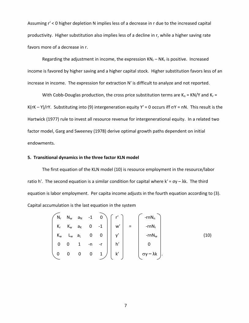
Assuming r′ < 0 higher depletion N implies less of a decrease in r due to the increased capital
productivity. Higher substitution also implies less of a decline in r, while a higher saving rate
favors more of a decrease in r.
Regarding the adjustment in income, the expression KNr – NKr is positive. Increased
income is favored by higher saving and a higher capital stock. Higher substitution favors less of an
increase in income. The expression for extraction N′ is difficult to analyze and not reported.
With Cobb-Douglas production, the cross price substitution terms are Kn = KN/Y and Kr =
K(rK – Y)/rY. Substituting into (9) intergeneration equity Y′ = 0 occurs iff Y = nN. This result is the
Hartwick (1977) rule to invest all resource revenue for intergenerational equity. In a related two
factor model, Garg and Sweeney (1978) derive optimal growth paths dependent on initial
endowments.
5. Transitional dynamics in the three factor KLN model
The first equation of the KLN model (10) is resource employment in the resource/labor
ratio h′. The second equation is a similar condition for capital where k′ = σy – λk. The third
equation is labor employment. Per capita income adjusts in the fourth equation according to (3).
Capital accumulation is the last equation in the system
Nr Nw aN -1 0 r′ -rnNn
Kr Kw aK 0 -1 w′ = -rnNr
Kw Lw aL 0 0 y′ -rnNw (10)
0 0 1 -n -r h′ 0
0 0 0 0 1 k’ y – λk .
8
For simplicity n′ and c′ are omitted in the system (10) but can be derived. The increase in the
resource price is derived from the optimal depletion condition according to n′ = rn. Consumption
is tied directly to income in the condition c′ = (1 – σ)y′.
The comparative static system solves for endogenous instantaneous changes in the capital
return r′, wage w′, per capita income y′, resource/labor ratio h′, and capital/labor ratio k′. These
directions of change depend on substitution as well as the levels of inputs, output, and factor
prices. Regularity conditions in production restrict substitution according to
d1 NnKr – Nr2 > 0 d2 NnLw – Nw
2 > 0 d3 KrLw – Kw2 > 0 (11)
d4 NwNr – NnKw > 0 d5 NrKw – KrNw > 0 d6 NwKw – NrLw > 0.
The sign of the determinant Δ = -n(aNd3 + aLd5 + aKd6) + d3 depends on substitution as well as unit
input levels and the resource price n. Instability of the system with a zero determinant is a global
issue. The present paper assumes local stability.
Including the condition for capital deepening, cofactors of solutions for endogenous
variables are
r’ = r[-n2(aKd2 + aLd4 + aNd6) – nd6 + k’(aLKw – aKLw)]
w’ = r[-n2(aLd1 + aKd4 + aNd5) + nd5 – k’(aLKr – aKKw)] (12)
y’ = r[n2(Nnd3 + Nwd5 + Nrd6) + k’d3]
h’ = r[n(Nnd3 + Nwd5 + Nrd6) + k’(aNd3 + aLd5 + aKd6)].
Each may be positive or negative, but there are presumptions that r’ < 0, w’ > 0, y’ > 0, and h’ < 0.
Assuming a negative determinant, a higher saving rate implies a larger k’ with a smaller r’ and
larger w’ and y’.
The following simulations do not exhaust possibilities but provide some insight into model
dynamics. With no loss of generality, scale inputs and output to one implying unit inputs ai = 1.
9
Assume σ = 0.12 and λ = 0.02 implying k´ = 0.1. Focus on resource substitution assuming Kw = 1
with Cobb-Douglas substitution between capital and labor. Assume the factor price vector (w, r,
n) = (0.4, 0.4, 0.2) that equals factor shares with the scaling. Suppose Nr = 1 and let Nw vary from
substitutes to complements. If Nw = 0.5 the vector of endogenous adjustments is (r´, w´, y´, h´) =
(0.86, 0.84, 0.36, 1.32). The rising resource price increases labor demand, raising the wage.
Demand for capital increases as does the capital return in spite of capital deepening. Income per
capita rises. The resource/labor ratio increases as extraction outpaces labor growth. If the
resource and labor are complements with the substitution term Nw = -0.5, the adjustment vector
is (0.22, 0.17, 0.08, -0.11). The rent and wage increase but much less than when the resource and
labor are substitutes. There is very little increase in per capita income. The resource/labor ratio
falls consistent with the smaller increase in the rent and wage.
Now consider substitution between the resource and capital in the Nr term. Assume Kw = 1
and Nw = 0.1. If Nr = 1 the vector of adjustments is (0.42, 0.40, 0.16, 0.30). If Nr equals -0.1 the
vector is (0.50, 0.40, 0.09, -0.07). With less substitution for capital, the rising resource price
implies more of an increase in capital rent and a diminishing resource/labor ratio.
Intergenerational equity with y’ = 0 is satisfied only if n2(Nnd3 + Nwd5 + Nrd6) = -k’d3, a
completely accidental condition. Investing resource rent is not relevant to intergenerational
equity. At any rate, developing economies would target rising per capita income. In practice,
knowledge of production is essential with no simple rule to follow for intergenerational equity.
6. The tragedy of the commons and a myopic nonrenewable resource owner
Common pool ownership leads to the tragedy of the commons with over-depletion of the
nonrenewable resource. There is no profit from extraction as owners of the common pool drive
price to marginal extraction cost MEC. For simplicity, assume MEC = 0, implying the clear tragedy
10
where n = 0 = n′. The comparative static model with common pool ownership is then similar to
(10) with n equal to 0 and the exogenous vector all zeroes except for the last term y - λk. The
wage and capital return could rise or fall. Depletion per capita grows with the capital/labor ratio
according to h′ = rk′. Depletion N′ = (h′ + h)L increases if h′ > -h.
A myopic monopoly resource owner maximizes immediate profit disregarding the asset
value of the stock, setting marginal revenue MR equal to marginal extraction cost MEC. Total
resource revenue is nN implying MR = ∂(nN)/∂N = n + N(∂n/∂N) = n + N(n′/N′). If MEC = 0 it
follows that n′N = -nN′ with depletion offsetting the rising resource price. Constant MEC would
imply constant marginal profit. The change in the resource/labor ratio is h′ = N′/L – λh. Myopic
extraction N′ = -n′N/n implies h′/h = -(n′/n + λ). Assuming no labor growth, the resource input
offsets price implying a constant resource share of income. Labor growth would imply a falling
resource share, the result of disregarding future resource revenue.
8. Conclusion
A nonrenewable resource added to capital and labor in the neoclassical growth model
introduces its own dynamics and increases the potential effects of substitution on growth and
income distribution. Depletion may intermittently increase along the growth path, even when the
resource price is rising. The wage may fall and the capital return may rise, even with capital
deepening. Adjustments along the growth path are determined by the pattern of substitution as
well as the levels and prices of the three inputs. Unlike the two factor model, investing resource
rent is irrelevant to maintaining per capita income.
The present three factor growth model provides a foundation for economic growth and
macroeconomics for countries rich in nonrenewable resources. Simulations of the present model
would reveal the evolution of depletion and income distribution for particular production

11
functions, initial endowments, saving propensities, and labor growth rates. Model simulations can
also examine global stability. Simulated growth paths can reveal turning points in depletion and
income distribution as well as switch points to backstop renewable resources. Another extension
of the model would be to open the economy to an exogenous international resource price.
12
References
Allen, R.G.D. (1938) Mathematical Analysis for Economists, New York: St. Martin's Press Barro, Robert and Xavier Sala-i-Martin (1999) Economic Growth, Cambridge: The MIT Press Dasgupta, P.S. and G.M. Heal (1974) The optimal depletion of exhaustible resources, Review of Economic Studies, 3–28
Dixit, A., P. Hammond, and M. Hoel (1980) On Hartwick’s rule for regular maximin paths of capital accumulation and resource depletion, Review of Economic Studies 47, 551-6 Faber, Malte and John Proops (1993) Natural resource rents, economic dynamics and structural change: A capital theoretic approach, Ecological Economics 8, 17-44
Farzin, Y.H. (1999) Optimal saving policy for exhaustible resource economies, Journal of Development Economics 58, 149-84
Garg, Prem and James Sweeney (1978) Optimal growth with depletable resources, Resources and Energy 1, 43-56 Hamilton, Kirk (1995) Sustainable development, the Hartwick rule, and optimal growth, Environmental and Resource Economics 5, 393-411 Hartwick, J. (1977) Intergenerational equity and the investing of rents from exhaustible resources, American Economic Review 66, 972-74 Hartwick, J. (1990) Natural resources, national accounting and economic depreciation, Journal of Public Economics 43, 291-304 Hotelling, H. (1931) The economics of exhaustible resources, Journal of Political Economy 39, 137-75 Jones, Ron and Stephen Easton (1983) Factor intensities and factor substitution in general equilibrium, Journal of International Economics 15, 65-99 Robinson, T. J. C. (1980) Classical foundations of the contemporary economic theory of nonrenewable energy resources, Resources Policy 6, 278-89 Sato, Ryuzo and Youngduk Kim (2002) Hartwick's rule and economic conservation laws, Journal of Economic Dynamics and Control 26 437-49 Solow, Robert (1956) A contribution to the theory of economic growth, Quarterly Journal of Economics 70, 65-94
13
Solow, Robert (1974) Intergenerational allocation of natural resources, Review of Economic Studies 41, 29-45 Stiglitz, Joseph (1974) Growth with exhaustible natural resources: Efficient and optimal growth paths, Review of Economic Studies, 123–37 Swan, Trevor (1956) Economic growth and capital accumulation, Economic Record 32, 234-61 Takayama, Akira (1982) On theorems of general competitive equilibrium of production and trade: A survey of recent developments in the theory of international trade, Keio Economic Studies 19, 1-38 Takayama, Akira (1993) Analytical Methods in Economics, Ann Arbor: University of Michigan Press Thompson, Henry (1985) Complementarity in a simple general equilibrium production model, Canadian Journal of Economics 18, 616-21 Thompson, Henry (2006) The applied theory of energy substitution in production, Energy Economics 28, 410-25.
Withagen, Cees and Geir B. Asheim (1998) Characterizing sustainability: The converse of Hartwick's rule, Journal of Economic Dynamics and Control 23, 159-63


![Nonrenewable energy[1]](https://img.dokumen.tips/doc/110x75/558c1703d8b42aab558b4626/nonrenewable-energy1.jpg)


