Embed Size (px)
Citation preview

A SIMPLE MODEL FOR ESTIMATING THE BOWEN RATIO FROM CLIMATIC
FACTORS FOR DETERMINING LATENT AND SENSIBLE HEAT FLUX
Corresponding author:
Pedro J. Perez
Dpto. de Medio Ambiente y Ciencias del Suelo, Universidad de Lleida.
Av. Rovira Roure, 191. 25198 - Lleida, Spain.
E-mail adress: [email protected]
Tel.: +34 973 702614
Fax: +34 973 702613
1
A SIMPLE MODEL FOR ESTIMATING THE BOWEN RATIO FROM CLIMATIC
FACTORS FOR DETERMINING LATENT AND SENSIBLE HEAT FLUX
P.J. Perez(1), F. Castellvi(1) and A. Martínez-Cob(2)
(1) Dpto. de Medio Ambiente y Ciencias del Suelo, Universidad de Lleida. Av. Rovira Roure, 191,
25198 Lleida, Spain.
(2) Laboratorio de Agronomía y Medio Ambiente (DGA-CSIC), Dpto. de Genética y Producción
Vegetal (EEAD), Apdo. 202, 50080 Zaragoza, Spain.
ABSTRACT
The energy partitioning or Bowen ratio $ at the surface, can be expressed as a function of a climatic
factor C (which depends on the climatic characteristics through the climatological resistance r i) and of
a surface factor S (which depends on the surface characteristics through the surface resistance rc). This
paper explains an approach for estimating S and therefore $ as a function of standard meteorological
variables. The empirical approach is then validated by estimating the latent (8E) and sensible (H) heat
flux. The experimental data were measured over grass at two semiarid locations in the Ebro river
valley, NE Spain, with typical Mediterranean climates: at Mas Bove, using a Bowen ratio-energy
balance method from 1991 to 1993, and at Zaragoza, using a weighing lysimeter from 1999 to 2000.
Results show that the surface factor S depends on the square root of the absolute value of r i/ra (where
ra is the aerodynamic resistance), with two locally calibrated empirical parameters. This result is valid
for the largest possible range of situations ($ values) throughout the day. Using three different
hypotheses for computing ra, results for $ (following hypothesis 1) indicate a good level of
performance by the model, although with a high degree of variability. The estimated latent heat flux
8Eest,1 tends to slightly underestimate the measured values. Under the semiarid conditions of the
region, 8EPM estimates obtained with the Penman-Monteith equation produce relative errors that are
greater than those obtained with the proposed model once it has been calibrated. On average, sensible
heat flux tends to be overestimated with the proposed method.
Keywords: Bowen ratio, energy partitioning, surface resistance, evapotranspiration, Penman-Monteith
equation

2
1. INTRODUCTION
Evapotranspiration is a component of the hydrological cycle whose accurate calculation at the
local and regional scales is needed to achieve an appropriate management of water requirements. A
high degree of precision in estimating crop evapotranspiration may permit important water savings in
the planning and management of irrigated areas. In 1977, the Food and Agriculture Organisation
(FAO) proposed a methodology for computing crop evapotranspiration based on the use of reference
evapotranspiration (ETo) and crop coefficients (Kc). Allen et al. (1998) redefined the concept of ETo
and adopted the Penamn-Monteith (PM) equation with constant canopy resistance (rc) to estimate ETo.
The PM model combines the energy balance with the expressions that describe heat fluxes to
derive a method for estimating the vapour flux from a vegetated surface. It has been applied in
different regions of the world and has provided better results over the reference crop than using other
approaches (Kustas et al., 1996; Monteith and Unsworth, 1990; Jensen et al., 1990; Allen et al., 1998;
Hussein, 1999; Pereira et al., 1999; Ventura et al., 1999). Later studies involving the PM equation
have also suggested the underestimation of the high measured values of ETo in semiarid and windy
areas, with a high evaporative demand, and overestimation in cases with low ETo values (Steduto et
al., 2003; Lecina et al., 2003; Todorovic, 1999; Rana et al., 1994).
When using the PM equation in a one-step approach, two kinds of parametric data must be
known: aerodynamic resistance ra (s m-1) and bulk canopy or surface resistance rc (s m-1) to water
vapour transport. On the basis of turbulent transfer and assuming a logarithmic wind profile, ra can be
calculated from the top of the canopy (hc) to the reference height through commonly used formulations
(Hall, 2002; Alves and Pereira, 2000; Pereira et al., 1999; Alves et al., 1998; Verhoef, 1995; Perrier,
1975). The net resistance to diffusion through the crop and soil surfaces, is represented in the PM
model by the bulk surface resistance rc. It is therefore not only a physiological parameter but also has
an aerodynamic component (Lhomme, 1991). It is not easy to estimate rc for different climatic and
crop water conditions, as it is influenced by solar radiation, temperature, vapour pressure deficit and
soil water content (Alves et al., 1998; Huntingford; 1995; Kim and Verma, 1991; Jarvis, 1976).
3
Several authors have developed simple methodologies for modelling rc as a linear function of
a climatic resistance r i. The value of r i mainly depends on climatic characteristics influenced by net
radiation Rn, soil heat flux G and air vapour pressure deficit. The model has been applied to wheat
(Perrier et al., 1980), grass and alfalfa (Steduto et al., 2003; Lecina et al., 2003; Rana et al., 1994;
Katerji and Perrier, 1983), tomato (Katerji et al., 1988) and lettuce (Alves and Pereira, 2000). These
empirical relationships of the form )/(/ aiac rrbarr += , make it possible to estimate rc using only
standard meterorological variables, although the parameters a and b must be empirically calibrated.
Alves and Pereira (2000) have shown that these parameters actually depend on the temporary value of
the Bowen ratio $, the only factor that is not readily available. Therefore, for practical purposes the
Bowen ratio needs to be estimated. However, for well-watered crops and over short periods of time $
is not expected to exhibit large variations, unless solar radiation varies drastically.
The partitioning between latent 8E and sensible H heat flux, that is, the Bowen ratio $ =
H/8E, is critical in determining the hydrological cycle, boundary layer development, weather and
climate. The surface resistance for a vegetated surface plays an important role in determining how the
available energy Rn-G is partitioned between H and 8E, as $ can be interpreted as an indicator of water
stress. The process of accommodation of plants to water demand is coupled with that of thermal
accommodation in the lower atmosphere (Monteith, 1995). The behaviour of stomata in response to
the environment is seen as a physiological response. The response to radiation is linked to the process
of photosynthesis and this is the basis for optimizing models of stomatal resistance. It seems that the
dependence between the energy partitioning $ and rc shows that attention should focus on estimating
and quantifying the energy partitioning (Alves and Pereira, 2000; Wilson et al., 2000).
At the surface, energy partitioning is a complex function of interactions between plant
physiology and the development of the atmospheric boundary layer. The Bowen ratio can be
expressed as (Wilson et al., 2002; Lockwood, 1979):
a
i
a
i
a
c
r
rr
r
r
r
+∆
−+=
γ
β1
(1)
where the climatological resistance r i is (Monteith, 1965)
)()(
)( *
GR
Dc
GR
eecr
n
pa
n
pai −
=−
−=
γρ
γρ
(2)

4
Da is the mean air density at constant pressure (kg m-3), cp is the specific heat of moist air at constant
pressure (1004 J kg-1 ºC-1); e* and e are respectively the saturation and actual vapour pressure of the air
(Pa), and D = e*-e (Pa) the atmospheric vapour pressure deficit; ( is the psychrometric constant (Pa
ºC-1) and ) is the slope of the saturation vapour pressure curve with respect to temperature (Pa ºC-1);
Rn and G are respectively the net radiation and soil heat flux and Rn - G the available energy (W m-2).
The objective of this work is to estimate the Bowen ratio from a surface factor and a climatic
factor using standard meteorological data, and to apply this method to estimate latent and sensible heat
flux. Equations (1) and (2) illustrate that the partitioning of turbulent energy fluxes is a function of
atmospheric demand through r i, turbulent transport through ra, surface resistance rc and air
temperature through ). The model presented below seeks to satisfy two different objectives. Firstly, it
seeks to offer an approach for estimating a surface factor S, depending on surface resistance rc, as a
function of standard meteorological variables. Secondly, the method seeks to evaluate the magnitude
of the Bowen ratio and the ability of the model to estimate latent and sensible heat fluxes at the
surface. Climate models including rc and $ variability may improve the calculated surface energy
fluxes in studies of future climate change.
2. MODEL
The partition of energy at the surface between sensible and latent heat flux is usually obtained
by the Bowen ratio-energy balance method (Perez et al., 1999; Kustas et al., 1996) by means of the
Bowen ratio
E
H
λβ = (3)
The Bowen ratio combined with the surface energy balance equation, which for uniform surfaces can
be simplified to
EHGRn λ++= (4)
yields the following expressions for 8E and H
)(1
1GRE n −
+=
βλ (5)
)(1
GRH n −+
=β
β (6)

5
Over an averaging period (traditionally 30 min), empirical relationships between fluxes and
vertical gradients can be formulated as
z
TkcH
z
ek
cE hpav
pa
∂∂−=
∂∂−= ρ
γρ
λ , (7)
Assuming kh = kv (Verma et al., 1978) and taking measurements between two levels within the
adjusted surface layer, $ is obtained as
e
T
ze
zT
∆∆=
∂∂∂∂= γγβ
/
/ (8)
where )T and )e are the temperature and vapour pressure differences between the two measurement
levels. This technique allows us to obtain 8E and H from Eqs. (5) and (6) when the available energy
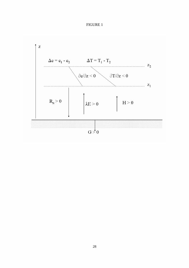
(Rn - G) is accurately measured. The convention used for the energy flux signs is Rn positive
downward and G positive when it is conducted downward from the surface (Fig. 1). Latent and
sensible heat fluxes are positive upward for negative vapour pressure and temperature gradients (Eq.
7). Any advection term in Fig. 1 has been omitted according to the simplified energy balance (Eq. 4).
The K-theory assumes that the turbulent transfer coefficients for heat and water vapour are
identical, which is not always true, particularly under conditions of local advection. In this case, an
incomplete adjustment of the fluxes within the internal boundary layer may cause deviations from
unity of the turbulent coefficient ratio kh/kv. Results reported by different authors are often
contradictory but, despite this, assuming kh = kv and using the Bowen ratio method to calculate surface
energy fluxes will usually only result in minor errors (McNaughton and Laubach, 1998). Moreover,
Eq. (8) is often limited to short canopies due to fetch requirements (Stannard, 1997) and large errors in
8E can occur when the Bowen ratio $ . -1 such as near sunrise and sunset (Perez et al., 1999).
Another of the methods based on flux-gradient theory and commonly used to estimate 8E is
the Penman-Monteith (PM) combination model, which represents a basic general description of the
evaporative process from a vegetative surface. However, in this method the water vapour flux is from
the canopy or vegetated surface to a level above the canopy, rather than between two heights above the
surface (Drexler et al., 2004). The PM model is expressed as (Allen et al., 1998):
)1(
/)()( *
a
c
apan
r
r
reecGRE
++∆
−+−∆=
γ
ρλ (9)

6
where 8E is the latent heat flux density (W m-2), Rn and G are respectively the net radiation and soil
heat flux (W m-2), ra is the aerodynamic resistance (s m-1) and rc is the canopy or bulk surface
resistance (s m-1). ra is the resistance to the turbulent transfer of vapour between the source and the
reference level. For homogeneous canopies, the source of water vapour and heat is located at height
d+zoh, which is considered the effective crop surface (Allen et al., 1998), where d (m) is the zero-plane
displacement and zoh (m) is the roughness length for heat. rc is the bulk surface resistance of the entire
vegetation canopy considered as a 'big leaf' (taken as the parallel sum of the stomatal resistances) or
simply the canopy resistance.
Over a very large, homogeneous, moist surface and under steady conditions, e tends to the
saturation value e* and rc << ra. Consequently, the first term on the right hand side in Eq. (9)
dominates, and in that case Eq .(9) (with rc . 0) describes the 'equilibrium' evaporation conditions
(Pereira et al., 1999; Monteith and Unsworth, 1990)
)( GRE ne −+∆∆=
γλ (10)
Eq. (10) may be considered as the lower limit of evaporation from moist surfaces. The aerodynamic
term, or second term on the right in Eq. (9), is therefore a measure of the departure from equilibrium in
the atmosphere. The atmospheric boundary layer is hardly ever uniform and tends to maintain a
humidity deficit, even over oceans. Thus, equilibrium is rarely observed over a wet surface and the
success of the PM model for estimating evapotranspiration may depend on the accuracy of modelling
average surface resistance rc.
The prior Eq. (9) can be written in the form
a
c
n
apan
r
r
GR
reecGR
Eγγ
ρ
λ++∆
−∆−
+−∆
=)(
)(
/)(1)(
*
and, taking the equilibrium evaporation expression (Eq. (10)) as a common factor and rearranging
terms, the above expression can then be rewritten as
a
c
an
pa
n
r
rrGR
eec
GRE
γγ
ρ
γλ
+∆+
−∆−
+−
+∆∆=
1
)(
)(1
)(
*
(11)

7
On the right-hand side of the expression, the numerator can be expressed in the same form as
the denominator, by defining a climatological resistance r i (Monteith, 1965) given by Eq. (2), so that,
through substitution in Eq. (11) we obtain
a
c
a
i
n
r
rr
r
GRE
γγ
γ
γλ
+∆+
∆+
−+∆∆=
1
1
)( (12)
The value for climatological resistance depends on the specific climatic characteristics, although Rn
and G are also influenced by the characteristics of the vegetative surface. This r i can be considered as
the upper limit of surface resistance, since Eλ tends to eEλ in Eq. (12) for a specific value for the
surface resistance [ ] iec rrr ∆+∆=≡ )( γ . For non-saturated surfaces under normal or dry conditions is
eEE λλ ≥ and then ec rr ≤ (Pereira et al., 1999; Culf, 1994; De Bruin and Holtslag, 1982). It therefore
seems advisable to analyse rc as a function of r i for land surfaces covered with homogeneous
vegetation where there is not shortage of water.
Equation (12) depends on time, but in practice meteorological variables are continuously
measured and averaged on a half-hourly or hourly basis, so the PM model can still be applied. The
fraction on the right-hand side of Eq. (12) is a dimensionless quantity that mainly depends on climatic
(through r i) and surface (through rc and ra) characteristics. Therefore Eq. (12) can be written as
S
CGRE n +
+−+∆∆=
1
1)(
γλ (13)
where C and S
a
i
r
rC
∆= γ
, a
c
r
rS
γγ+∆
= (14)
are dimensionless and are respectively referred to as the climatic factor and surface factor.
When the big leaf model expressed by Eq. (13) is combined with Eq. (5), the Bowen ratio can
be obtained as
11
1 −++
∆+∆=
C
Sγβ (15)
This expression is equivalent to that obtained by Wilson et al. (2002). Eq. (15) toghether with Eqs.
(14) show that the partitioning of surface turbulent energy fluxes is a function of: atmospheric demand
through climatic factor C (which is sensitive to available energy Rn-G and vapour pressure deficict D);

8
surface resistance to water vapour transport (rc) through surface factor S; turbulent transport through ra
and air temperature through ).
The climatic C and the surface S factors control β. However, results reported in the literature
(Lockwood, 1979; Wilson et al., 2000, 2002) indicate some general differences, mostly between
maritime and continental climates. Large-scale differences in climate influence atmospheric demand,
so more continental sites will tend to be drier and to have a higher D relative to Rn-G (large C and may
be low $). Maritime sites will tend to be cooler and more humid resulting in a lower D relative to Rn-G
(small C and perhaps high $). But the response of rc and therefore of S to changes in atmospheric
demand (stomatal resistance often increases with an increase in D), may compensate for factors S and
C in control β (Kelliher et al., 1995).
In an agricultural region with well-defined climatic characteristics (such as the semiarid
continental zone of this study), the climatic factor C could be expected to be constant for the entire
region and to be representative of the whole climatic zone. Thus, in order to extrapolate Eq. (15) to the
whole climatic region, the next step would be to analyse surface factor S and suggest some operational
approaches for estimating S and therefore β as a function of standard meteorological variables.
3. MATERIALS AND METHODS
3.1. Experimental data and site description
This study was conducted at two locations that are representative of the Ebro river basin: at
Zaragoza (41º 43’ N, 0º 49’ W, 225 m asl), in the central area of the valley, and at Mas Bove (41º 9'
N, 1º 10' E, 76 m asl) in the Mediterranean area (Fig. 2). In the case of the central Ebro site, the study
was conducted at an experimental farm located on the terraces of the river Gállego, in Zaragoza
province, about 8 km north of its confluence with the river Ebro. The site is located in one of the
windiest areas in Spain which has semi-continental climatic characteristics. The zone is a semiarid
region (average annual precipitation about 330 mm) but with important water resources. Precipitation
is mostly recorded in spring and autumn, though storm precipitation is also relatively frequent during
summer. Average annual temperature is about 15 ºC. Measurements were taken over a 1.2 ha plot with
uniform grass cover (Festuca arundinacea Moench.). The plot was regularly irrigated and cut
throughout the year to maintain it as near as possible to the reference standard.
9
A weighing lysimeter, 1.7 m in depth and covering an effective surface area of 6.3 m2, was
located at the centre of the plot. A load cell connected to a datalogger (CR500, Campbell Sci. Inc.)
recorded lysimeter mass losses at 0.5 s intervals. These data were used to derive hourly
evapotranspiration rates. The combined resolutions of the load cell and the datalogger made it possible
to detect mass losses of about 0.3 kg (0.04 mm water depth). Measurements were taken from March to
October 1999 and from March to September 2000. Only days without incidences (irrigation, rainfall,
lysimeter drainage and grass cutting), and when measured grass height was between 0.10 and 0.15 m
were used for analysis. An automatic weather station (CR10, Campbell Sci. Inc.) that was close to the
lysimeter recorded hourly average air temperature, relative humidity and net radiation at a height of
1.5 m. Wind speed and direction were measured at a height of 2.0 m. Soil heat flux was measured
using two plates buried at a depth of 8 cm and with an averaging soil temperature probe placed at a
depth of between 2 and 6 cm (Allen et al., 1996).
In the case of the Mediterranean site, data were collected in the period from August 1991 to
March 1993 using the Bowen Ratio-energy balance method at an experimental farm located at Mas
Bove, in the Ebro River basin; the site was 12 km from the Mediterranean coast. The average annual
precipitation at the site is below 520 mm. The main climatic characteristic is that maximum
precipitation occurs in autumn. Other local characteristics are temperate winters, warm summers and
humidity values ranging from 65% to 75% throughout the year (Castellvi et al., 1996).
The BREB was located on plots of festuca rye-grass sprinkler-irrigated. The grass height was
maintained between 0.10 and 0.15 m during the measurement periods. The equipment (Bowen-ratio
system, Campbell Scientific Inc.) whose detailed description can be found in the literature (Tanner et
al., 1987; Fritschen and Simpson, 1989), measures the gradient of air temperature by means of
unaspirated chromel-constantan thermocouples, and the vapour pressure gradient with a single cooled-
mirror dew-point hygrometer. Net radiation and soil heat flux were measured with a net radiometer
and heat flux plates respectively (Allen et al., 1996). The data were averaged over 30 minutes.
3.2. Method for estimating the surface factor S and the Bowen ratio β.
Based on the results obtained by Perrier et al. (1980) several authors (Katerji and Perrier,
1983; Rana et al., 1997, 1994; Alves and Pereira, 2000) proposed a model in which an empirical
relationship of the form )/(/ aiac rrbarr += exists between surface rc and climatological r i resistance.

10
Since rc depends on the source, coefficients a and b depend on the type of crop, on its phenological
state or on soil water status (Rana et al., 1997). Some of these experimental results referred to
reference crops such as grass and alfalfa grown in a Mediterranean climate (Steduto et al., 2003; Rana
et al., 1994; Katerji and Perrier, 1983), wheat (Perrier et al., 1980), tomato (Katerji et al., 1988) and
rice (Peterschmitt and Perrier, 1991). In these approaches, parameters a and b must be empirically
calibrated (Alves and Pereira, 2000).
Taking the Katerji and Perrier (1983) approach as a reference, it is possible to explore any
linear model that relates surface factor S to r i. The aim of this work was to find the best approach for
making estimations based on global empirical parameters, that are valid for any range of β values. If
they do exist, these parameters would be representative of the crop for any climatic conditions. In
order to analyse this simple model, we propose exploring a functional relationship of the form
+
+∆=
+∆= )(
a
i
a
cest r
rfba
r
rS
γγ
γγ
(16)
for the reference crop, where a and b are global parameters that are to be determined empirically. With
S estimated empirically from Eq. (16), we can estimate β (Eq. 15) as a function of standard
meteorological variables.
In the most commonly used formulations, aerodynamic resistance ra is estimated by
considering that apparent sources of heat and vapour within the canopy are at a lower level than the
apparent sink of momentum (Monteith and Unsworth, 1990). In the 'big leaf' model the big leaf is
implicitly located at the height d + zoh, where zoh (m) is the roughness length for sensible heat transfer.
When the leaves at the top of the canopy, between d + zoh and crop height hc, are the most important
source of vapour flux, the use of the d + zoh level as the evaporative surface can lead to an
overestimation of ra and to negative values for bulk surface resistance rc when it is computed by
inverting the PM equation. Notwithstanding, Wilson et al. (2002) found that hypothetical errors in ra
of as much as 100% resulted in mean errors of only about 10% in the computed value of rc. In order to
ascertain whether the proposed approach for surface factor S (Eq. 16) is sensitive to aerodynamic
resistance, we therefore used several hypotheses to compute ra for the reference crop.
Hypothesis 1: ra is computed between the top of the canopy hc and the reference height in the
atmosphere (Alves et al., 1998; Perrier, 1975) as
zm
c
h
om
m
auk
dh
dz
z
dz
r21
lnln
−−
−
= (17)

11
(denoted hereafter as ra1) where zm and zh are respectively the wind and air temperature measurement
heights, hc is the crop height, k is the dimensionless von Karman constant, and uzm is the wind speed
measured at height zm. The term hc - d substitutes the roughness length for heat transfer used to
compute ra according to Allen et al. (1998).
Hypothesis 2: In this case, the method proposed to compute ra for the reference crop is that proposed
by Allen et al. (1998) for grass, in which ra is obtained as
zm
a ur
2082 = (18)
where uzm is the wind speed measured at height zm.
Hypothesis 3: In order to establish whether dependence on wind speed can be avoided, for grass ra is
considered with constant average values during the diurnal and nocturnal periods: it was therefore
considered as
≤>
= −
−
)0(70
)0(901
1
3n
na
Rsm
Rsmr (19)
The experimental or measured hourly values of surface resistance rc (s m-1) were obtained by
inverting the PM equation (top-down approach) as
E
Dc
E
GRrr pnac λγ
ργ
γλγ
+
+∆−−∆= (20)
where 8E is the latent heat flux (W m-2) measured by a lysimeter (Zaragoza) or by a Bowen ratio
system (Mas Bove). Hourly values measured for Rn-G, D, u and 8E were used to compute hourly rc
values with Eq. (20), aerodynamic resistances with Eqs. (17) to (19) and climatological resistances
with Eq. (2). In the PM equation (Eq. 9), hereafter denoted as 8EPM, units and computations followed
Allen et al. (1998), rc was considered constant and equal to 70 s m-1 and grass height was set to 0.12
m.
For the present analysis, the data set available for each location was divided into two groups: a
calibration data set and a validation data set. Available days were organised by date and one of three
days was selected for calibration, while the other two were selected for validation. Using only the
calibration data sets from both locations, we subsequently explored several simple relationships
between rc/ra and r i/ra for Eq. (16).

12
3.3. Statistical methods
In the evaluation of the different relationships represented by Eq. (16), the ability to predict S
was compared using the coefficient of determination R2 as the measure of the goodness of fit, that is,
of the performance of the model; R2 is a measure of the total variance accounted for by the model.
Parameters a and b in Eq. (16) are then obtained for the best fit using the calibration data set.
A complication may arise when the model that maximizes R2 for rc, fails to maximize this
value when predicting energy partitioning or evapotranspiration. Once the best parameterization of S
had been chosen and the optimum coefficient values in Eq. (16) had been found, comparisons between
measured $ and estimated $est values were carried out. To test the performance of the resulting
approach, a simple linear regression between the predicted and observed values was made, based on
the value of R2. However, in order to make a better quantitative comparison between the models for
8E, predicted results could also be evaluated with reference to several statistics (Alexandris and
Kerkides, 2003; Lee and Singh, 1998; Verhoef et al., 1997; Mayer and Butler, 1993; Willmot, 1981,
1982).
The first statistic is the bias or mean deviation error, [ ] nPOMBE ii /)(∑ −= . The second is
the root mean square error, ∑ −= nPORMSE ii /)( 2 , which is considered a better indicator of
model performance than the correlation statistics. They can be expressed as percentages of the mean
observed value (relative ORMSERMSE /100(%) = ). In the above expressions, Pi and Oi represent
the predicted (estimated) and observed (measured) values, n is the total number of data and O is the
mean of observed data. RMSE provides a measure of the total difference between the predicted and
observed values. The closer RMSE is to zero, the better the prediction.
The statistic that we will use as the model selection criterion is modelling efficiency (Lee and
Singh, 1998) defined as [ ] [ ]∑∑ −−−= 22 )(/)(1 OOPOEF iii , which is similar to the index of
agreement (Willmot, 1982). Modelling efficiency is a dimensionless statistic that measures the fraction
of the variance of the observed values which is explained by the model. It therefore provides a good
measure of the model's performance. The best model is the one in which the value of EF is closest to 1
and which has the lowest RMSE.

13
4. RESULTS AND DISCUSSION
The available data set for each location was divided into calibration and validation data. Using
only the calibration data sets, we explored several simple relationships between rc/ra and r i/ra for
estimating the surface factor S (Eq. 16). In order to select the appropriate data, we first considered
necessary to assess the consistency and reliability of both the calibration and validation data sets.
a. Data processing
For the two data sets (Zaragoza and Mas Bove) considered for this study, the measured values
of latent 8E and sensible H heat flux must be physically consistent with the flux-gradient relationship
(Fig. 1). In the experimental measurements we required an adequate fetch, in order to have confidence
that the heat fluxes were in equilibrium with the surface. Nevertheless, sometimes the measurements
can give incorrect signs for those fluxes, at least for the estimates provided by the BREB method
(Perez et al., 1999). We therefore scrutinized both datasets from a practical point of view before
considering them for analysis. The objective was to apply some set of criteria to select appropriate
data or to reject physically inconsistent data. When available energy Rn-G is positive (downward with
the convention used in Fig. 1), energy fluxes 8E and H are positive upward with a direction opposite
to that of the vapour pressure and temperature gradients (Eq. 7).
In the analysis of data, three different situations were observed (hereafter denoted as Cases 1,
2 and 3). Case 1 corresponds to data with 8E>0 and H>0, representing 40% of total data. Case 1 is
the usual for unstable conditions during the daytime (mainly from 07h to 19h) with values of available
energy Rn-G>0. The case denoted as Case 2 corresponds to hourly data values with 8E>0 and H<0
and represents 45% of total data. Of this 45%, one third appears during the day and even during the
central hours of the day. They are associated with a downward sensible heat flux with positive
temperature gradients, corresponding to periods just after irrigation or precipitation.
The remaining two thirds of Case 2 appear at sunset (18h-19h) in inversion conditions
(MT/Mz>0) and persist throughout the night and until sunrise. They are associated with low values of
latent heat flux and of available energy Rn-G (mainly between -70 and 70 Wm-2). An 8% of total data
corresponds to what we denoted Case 3: data with 8E<0 and H<0. These cases, which indicate
condensation, also appear at night under stable conditions. They are associated with positive and low
14
vapour pressure gradients and also with small negative values of Rn-G, usually within the range of
experimental errors. Data with 8E=0 or data with 8E<0 and H>0 represent the remaining 7%. These
data were directly excluded from the analysis as it was assumed that the air near the surface was not
supersaturated (Andreas and Cash, 1996; Andreas, 1989; Philip, 1987).
In order to select the appropriate data from the data sets, another constraint was also taken into
account. Eq. (10) shows that equilibrium evaporation 8Ee is a lower limit of evaporation from moist
surfaces. Combining Eq. (10) with Eq. (5), it can be seen that for equilibrium evaporation the Bowen
ratio tends towards an equilibrium value ∆= /γβe . Therefore, for unsaturated surfaces under normal
daytime conditions (incoming available energy Rn-G>0, evaporation 8E>0 and H>0, so that $>0), the
condition 8E$8Ee applied to Eq. (5) requires that $#$e. The equilibrium Bowen ratio $e is an upper
boundary for Bowen ratio values when there is evaporation 8E$0 (Andreas, 1989; Philip, 1987).
During condensation at the surface under conditions of nocturnal inversion and outgoing available
energy (8E<0 and H<0), 8Ee is an upper limit of latent heat flux and $e is a lower boundary for the
Bowen ratio, i.e., $e#$. These constraints on $ were added to Cases 1 and 3 and all of the criteria were
applied to our data sets. We then excluded the small percentage of data that did not fit into any of the
three cases.
b. Model calibration
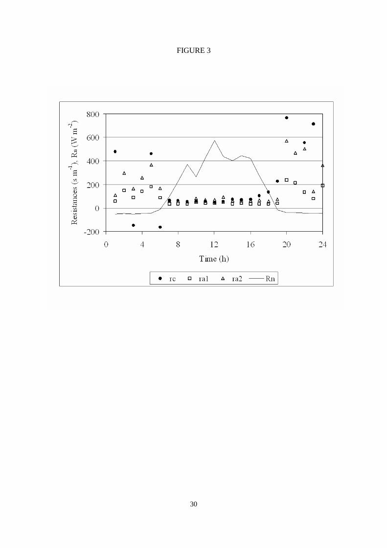
When we examined the behaviour of rc for Cases 1 and 2, we observed a similar degree of
diurnal variability to that shown in Fig. 3. Values of rc tend to remain relatively constant throughout
the diurnal period from 9h to 16h. But there was an observed fall in early morning values and then a
gradual increase in late afternoon. This pattern was also reported by other authors (Alves and Pereira,
2000) and reflects the daily course of the environmental variables affecting rc. The most important
factor were net radiation and variables like vapour pressure deficit (D) and temperature. The rise of rc
which was observed in late afternoon is consistent with the closure of stomata due to a decrease in
radiation (Fig. 3). Independently of the time of day, negative values were obtained for rc, but these
were mainly registered early in the morning and at night, when the available energy tends to be small
and negative and when the vapour pressure deficit is also small.
The response of rc to net radiation seems to indicate the need to consider data corresponding to
the diurnal period (Rn-G>0) separately from those corresponding to the nocturnal period (Rn-G#0).
The main drawback is that when Rn-G and D are low, such as at sunrise and sunset and during the

15
nocturnal period, the canopy rc and climatological r i resistances register either very high positive or
very low negative values. This also leads to very high positive or very low negative $ values. In
general, these results correspond to data with Rn-G within the range of experimental errors (20-30
Wm-2). Figure 4 shows the dependence of $ on r i/ra,; in it, it is possible to observe that $ = -1 is a
critical value to consider. It therefore seems that our attention should not focus on separate data in
diurnal and nocturnal values. The key to our analysis should center on the fact that the variability of $
versus r i/ra presents a simmetrical pattern with respect to the critical value $=-1.
This behaviour of $ led us to select two sets of data: one in which the data interval was $>-1
(subset '$>-1') and the other in which it was $<-1 (subset '$<-1') (Fig. 4). From a physical point of
view, the critical value $=-1 leads to non-defined values in 8E and H (Eqs. 5 and 6). It also produces
the change of sign from positive to negative values in the heat fluxes. In general, data with $<-1
correspond to the two thirds of nocturnal Case 2. On the contrary, data with $>-1 correspond to all
types of Cases 1, 2 and 3, appearing in both the diurnal and nocturnal periods, as well as with positive
and negative values of available energy.
Our objective is to try to find the best empirical relationship between rc/ra and r i/ra that
provides us with an approach for estimating the surface factor S (Eq. 16) and then the Bowen ratio $
(Eq. 15). Results reported by others authors (Steduto et al., 2003; Alves and Pereira, 2000; Rana et al.,
1997) seemed to show a linear relationship between rc/ra and r i/ra on an hourly basis. But these results
were generally obtained for a limited range of $ values throughout the diurnal period. Alves and
Pereira (2000) found such results for $ values in the interval [-0.3, 0.3], corresponding to situations
when crop evapotranspiration was at its maximum and when available energy Rn-G had values
corresponding to the middle of the day. Previously found results obtained for our semiarid region
using the same methodology (Perez et al., 2006), showed that the functional form of the dependence of
rc/ra on r i/ra departs from linearity. The response of rc/ra tends towards saturation when r i/ra increases
(Fig. 5). Since we have included the largest possible range of situations throughout the day, these
results effectively extend those reported by other authors.
Within the global calibration data set for the two measurement zones, each data subset was
analysed separately. For subset '$>-1', low values of Rn-G at sunrise, sunset or during the night,
produced imprecise values of rc and r i (very high positive or very low negative values) and therefore
led to an imprecise calibration. For subset '$<-1' all data appeared during the night with small negative
Rn-G values in the interval [-60, -1] (W m-2), and with low values of r i<0. A typical error associated
with the measurement of net radiation is "5%, and the resolution of the weighing lysimeter is 0.04 mm
16
(.30 W m-2) in the measurement of evapotranspiration. To avoid large errors in the computed surface
and climatological resistances, all the calibration data with *Rn-G*#10 W m-2 were excluded from the
analysis independently of $ values.
For the global calibration data set, Figure 5 shows the measured and estimated values of rc/ra
versus r i/ra after calibration obtained according to hypothesis 1. For subset '$>-1' (Fig. 5, right) data
correspond mainly to the diurnal period with Rn-G $10 W m-2, r i>0 and $ values in the interval [-0.88,
0.86]. For subset '$<-1' (Fig. 5, left) data correspond to the nocturnal period with Rn-G # -10 W m-2,
r i<0 and $ values in the interval [-5.3, -1.17]. Table 1 shows the values of the empirical coefficients
locally calibrated for the whole calibration data set. Our results confirmed the previously reported
(Perez et al., 2006), showing that the best-fit relationship corresponds to a dependence of rc/ra on the
square root of r i/ra. Subset '$<-1' showed a symmetrical behaviour respect to that of subset '$>-1', but
for negative values of r i/ra. This was demonstrated after separately applying the calibration obtained
for subset '$>-1' to subset '$<-1'. Results showed that the calibration is perfectly valid if the sign of r i
is previously changed. Calibration was therefore made in function of the absolute values of r i/ra (Table
1), so that the result could be applied to any range of $ values both during the diurnal and nocturnal
periods.
c. Model validation: estimation of Bowen ratio and heat fluxes
Differences in the values of empirical coefficients obtained under the different hypotheses
(Table 1) were due to aerodynamic resistance. The hourly values of ra1 obtained under hypothesis 1
(Eq. 17) were lower than those obtained using the method proposed by FAO (Allen et al., 1998) for
the reference crop ra2 (Eq. 18). On average, ra1 was half the value of ra2 as seen in Fig. 3 for any
typical day. This confirmed results obtained by other authors over both short and tall vegetation (Hall,
2002; Alves et al., 1998). According to Verhoef (1995), differences in the estimation of ra for dense or
sparse canopies or even for grass, are the result of problems associated with the parameterization of an
excess resistance.
The calibrated values of parameters a and b in Eq. (16) allowed us to obtain an estimated
surface factor Sest. This was applied to the validation data set, toghether with the climatic factor C (Eq.
14), to estimate hourly Bowen ratio values $est from Eq. (15), hourly latent heat flux values 8Eest from

17
Eq. (5) or Eq. (13), and sensible heat flux values Hest from Eq. (6). Estimated values $est were validated
throughout the study period for the global validation data set. Estimated values 8Eest were validated by
comparison with measured values 8E obtained using a weighing lysimeter (Zaragoza) and a Bowen
ratio system (Mas Bove). They were also compared to estimates 8EPM obtained by applying the
Penman-Monteith equation (Eq. 9).
Once empirical calibration was applied, the statistics used to validate the method for
estimating S and $ are reported in Tables 1 and 2. These results indicated that surface factor S was
estimated similarly under hypotheses 1 and 2 (modeling efficiency EF=0.6), but with a relatively high
RMSE of 70% (Table 2). When the estimated (rc/ra)est or Sest were compared with the experimental
values (Fig. 6), a higher scatter of data was observed for the high S values. As a consequence, the
proposed model led to an average underestimation of the surface factor (positive MBE) for the whole
validation data set. However, this result improved substantially when only the diurnal period (subset
'$>-1') was considered (positive S values between 0 and 2.2).
The climatic factor C and the surface factor S control the Bowen ratio $ (Eq. 15). The
response of C and S (or rc) to changes in atmospheric demand can therefore lead to a compensation of
both factors in the $ values. However, when $ is estimated from Eq. (15), it should be noticed that the
climatic factor C in the denominator leads to non-defined $ values for C . -1. These negative C
values around -1 only appear during the nocturnal period with negative available energy Rn-G<0
(r i<0). Therefore, prior to the validation of the model, all validaton data with C values belonging to the
interval [-1.1, -0.9] were excluded from the analysis.
Application of the model showed good performance for $ under hypotheses 1 and 2, with
high modeling efficiencies (Table 2). However, there was a high degree of variability, as indicated by
the RMSE = 104% for $est,1. As can be seen in Fig. 7, this was probably due to the higher errors
obtained for the nocturnal period (subset '$<-1'). There was a slight overestimation of $ under
hypothesis 1 (MBE=-8.3%) and a similar underestimation under hypothesis 3 (MBE=8.6%), but the
global comparison between estimated and measured values showed slopes of linear regression close to
1 (Table 2).
The variable values for S and $ estimated with the proposed model were used in Eqs. (5) or
(13) and (6), to respectively estimate the latent (8Eest) and sensible (Hest) heat flux values. Table 3
shows the results obtained for the global validation data set and for each hypothesis. Measured heat
fluxes 8E and H were obtained using a weighing lysimeter (Zaragoza) and a Bowen ratio system (Mas
18
Bove). For comparison purposes, latent heat fluxes 8EPM obtained with the Penman-Monteith equation
(Eq. 9), with a fixed value of rc = 70 sm-1, were also computed. The value of modelling efficiency for
8EPM (EF=0.95) showed good agreement for this method (Table 3). However, relative MBE and
RMSE were higher for 8EPM than for the proposed model 8Eest under any of the three hypotheses.
Simple linear regressions between estimated and measured 8E values showed that 8EPM displayed a
lower slope (c1=0.86) with respect to those obtained for 8Eest. This indicates the greater tendency for
8EPM to underestimate high latent heat fluxes under semiarid conditions (Fig. 8b). This behaviour has
already been reported in previous works carried out in the same region (Lecina et al., 2003; Perez et
al., 2006) and at other Mediterranean locations (Steduto et al., 2003; Rana et al., 1994).
For the proposed method, results of the comparison between estimated and measured fluxes
(Table 3) showed that the relative RMSE for 8Eest,1 was smaller than for hypotheses 2 and 3 and for
8EPM. The slope of the linear regression between 8Eest,1 and 8E (c1=0.97) was very close to 1, as can
be seen in Fig. 8. For 8Eest,2 and 8Eest,3, the slopes were closer to 1 than for 8EPM. Furthermore, the
small relative deviation error indicates that 8Eest,1 tended to slightly underestimate the measured
values, but in any case less than 8EPM does (Fig. 8). Toghether with the above results, the values for
the modeling efficiencies showed the good performance of the proposed method under hypothesis 1
for estimating $, 8E and H. Results obtained with 8Eest,2 were similar to those obtained with 8Eest,1 but
with a higher degree of variability.
With respect to the estimation of $ and sensible heat flux H, hypotheses 2 and 3 led to similar
results (Table 3) with high RMSE values. On average H was overestimated, as indicated by the
negative MBE, but the slopes of the linear regressions were close to 1 for Hest,1 and Hest,2 (Fig. 9a).
Hypothesis 3 may also be considered appropriate for estimating 8E and H. In particular for the
sensible heat flux, the values of modeling efficiency obtained were just a little lower than those
obtained under hypotheses 1 or 2. Comparison between Hest,3 and measured values of H showed good
agreement, particularly for the nocturnal period (subset of validation data with $ <-1) as can be seen in
Fig. 9b. It should also be noted that in hypothesis 3 aerodynamic resistance ra was taken as constant
(Eq. 19), and that wind speed is therefore not needed to estimate the surface factor Sest,3 or the Bowen
ratio $est,3. Taking into account this advantage and the results obtained, hypothesis 3 could also be
considered useful for estimating 8E and H under semiarid and windy conditions such as those found in
the Ebro river valley.

19
5. CONCLUSIONS
We explored an approach for estimating the surface factor S (Eq. 16) or the surface resistance
rc as a function of standard meteorological variables. This empirical approach was then applied for
estimating the Bowen ratio $ (Eq. 15) and the latent 8E and sensible H heat fluxes over grass (Eqs. 13
and 6, respectively). The issue is that when rc is calculated in a 'top-down' approach by inverting the
Penman-Monteith equation, the relationship obtained shows that rc depends on environmental
variables (Eq. 20). An approach for modeling rc or S as a function of climatic conditions, could
therefore be regarded as potentially useful for improving the estimation of energy partitioning $ and
surface energy fluxes.
Experimental results reported by other authors showed that, for a limited range of $ values
throughout the diurnal period, there is a linear relationship between rc/ra and r i/ra. For our semiarid
region with a Mediterranean climate, results obtained using the same methodology show that the
functional form of the dependence between rc/ra and r i/ra departs from linearity. The response of rc/ra
tends towards a certain saturation value when r i/ra increases. Using the calibration data set, the best
empirical approach for estimating S and $ on an hourly basis is a function of the square root of the
absolute value of r i/ra. This result is valid for any range of $ values: it includes the largest possible
range of situations encountered in the course of the day, thereby extending the results reported by
other authors.
The estimated surface factor Sest was applied to the validation data set, using three different
hypotheses for computing ra. Hourly values of Bowen ratio and latent and sensible heat fluxes were
thus estimated and validated by comparison with measured values. Results for $ indicate good
performance by the model under hypothesis 1, although with a high degree of variability. Estimated
latent heat flux performed relatively better under hypothesis 1 than under the other two hypotheses.
The small relative deviation error and root mean square error indicate that 8Eest,1 tends to slightly
underestimate measured values. Estimates 8EPM obtained with the PM equation lead to relative errors
that are larger than those obtained for the proposed model once it has been calibrated. There is a
tendency for 8EPM to underestimate the high latent heat fluxes under semiarid conditions.
Values for modeling efficiency indicate that the proposed method is appropriate for estimating
$, 8E and H under hypothesis 1. Although the improvement found in this work seems to be somewhat
limited, the estimation of evapotranspiration tends to perform better than the PM method with constant

20
rc. On average, sensible heat flux is overestimated with the proposed method. However, the estimated
values show good agreement with measured ones for the nocturnal period, even under hypothesis 3.
Since aerodynamic resistance is taken as constant in hypothesis 3, wind speed is not needed to
estimate the Bowen ratio $est,3.
The empirical approach for estimating the surface factor as a function of standard
meteorological variables can be considered potentially useful for estimating $, 8E and H under the
semiarid conditions of the Ebro river valley. This approach has the drawback that it requires local
calibration, but the small improvement observed in the estimation of 8E may contribute to produce
water savings.
Acknowledgements
This work was funded by the Spanish Ministry of Science and Technology under projects ENE2004-07619/ALT
and REN2001-1630/CLI and, and by the Department of Universities and Research (Generalitat de Catalunya)
under project 2001SGR-00306. The authors would like to thank Jesus Gaudó, Miguel Izquierdo and Enrique
Mayoral for their help with the fieldwork.

21
REFERENCES
Alexandris, S., Kerkides, P., 2003. New empirical formula for hourly estimations of reference
evapotranspiration. Agric. Water Manag. 60: 157-180.
Allen, R.G., Pruitt, W.O., Businger, J.A., Fritschen, L.J., Jensen, M.E., Quinn, F.H., 1996.
Evaporation and Transpiration. In: ASCE, Hydrology Handbook, 2nd ed., ASCE Manuals and Reports
on Engineering Practice no. 28, N.Y., p. 125-252.
Allen, R.G., Pereira, L.S., Raes, D., Smith, M., 1998. Crop evapotranspiration: guidelines for
computing crop water requirements. FAO Irrigation and Drainage Paper No. 56, FAO, Rome, 300 pp.
Alves, I, Perrier, A., Pereira, L.S., 1998. Aerodynamic and surface resistances of complete cover
crops: how good is the “big leaf”?. Trans. of the ASAE 41 (2): 345-351.
Alves, I., Pereira, L.S., 2000. Modelling surface resistance from climatic variables?. Agric. Water
Manag. 42: 371-385.
Andreas, E. L., 1989. Comments on a physical bound on the Bowen ratio. J. Applied Meteorol. 28:
1252-1254.
Andreas, E.L., Cash, B. A., 1996. A new formulation for the Bowen ratio over saturated surfaces. J.
Applied Meteorol. 35: 1279-1289.
Castellvi, F., Perez, P.J., Villar, J.M., Rosell, J.I., 1996. Analysis of methods for estimating vapor
pressure deficits and relative humidity. Agric. For. Meteor., 82(1-4): 29-45.
Culf, A.D., 1994. Equilibrium evaporation beneath a growing convective boundary layer. Bound.
Layer Meteor., 70: 37-49.
De Bruin, H.A.R., Holtslag, A.A.M., 1982. A simple parameterization of the surface fluxes of sensible
and latent heat during daytime compared with the Penman-Monteith concept. J. Appl. Meteor., 21:
1610-1621.
Drexler, J.Z., Snyder, R.L., Spano, D., Paw U, K.T., 2004. A review of models and
micrometeorological methods used to estimate wetland evapotranspiration. Hydrol. Process., 18:
2071-2101.
Fritschen, L.J., Simpson, J.R., 1989. Surface energy and radiation balance systems: general description
and improvements. J. Appl. Meteor. 28: 680-689.
Hall, R.L., 2002. Aerodynamic resistance of coppiced poplar. Agric. For. Meteorol. 114: 83-102.

22
Huntingford, C., 1995. Non-dimensionalisation of the Penman-Monteith model. J. Hydrol. 170: 215-
232.
Hussein, A.S.A., 1999. Grass ET estimates using Penman-type equations in Central Sudan. J. Irrig.
and Drain. Eng. 125 (6): 324-329.
Jarvis, P.G., 1976. The interpretation of the variations in leaf water potential and stomatal conductance
found in canopies in the field. Phil. Trans. Roy. Soc. London, Ser. B 273: 595-610.
Jensen, M.E., Burman, R.D., Allen, R.G. 1990. Evapotranspiration and Irrigation Water
Requirements. ASCE Manuals and Reports on Engineering Practice, No. 70. American Society of
Civil Engineers, New York, 360 pp.
Katerji, N., Perrier, A., 1983. Modélisation de l’évapotranspiration réelle d’une parcelle de luzerne:
role d’un coefficient cultural. Agronomie 3(6): 513-521.
Katerji, N., Itier, B. Ferreira, M.L., 1988. Etudes de quelques critères indicateurs de l’état hydrique
d’une culture de tomate en région semi-aride. Agronomie 5: 425-433.
Kelliher, F. M., Leuning, R., Raupach, M.R., Schulze, E.D., 1995. Maximum conductances for
evaporation from global vegetation types. Agric. For. Meteorol. 73: 1-16.
Kim, J., Verma, S.B., 1991. Modeling canopy stomatal conductance in a temperate grassland
ecosystem. Agric. For. Meteorol. 55: 149-166.
Kustas, W.P., Stannard, D.I., Allwine, K.J., 1996. Variability in surface energy flux partitioning
during Washita ’92: Resulting effects on Penman-Monteith and Priestley-Taylor parameteres. Agric.
For. Meteor., 82: 171-193.
Lecina, S., Martinez-Cob, A., Perez, P.J., Villalobos, F.J., Baselga, J.J., 2003. Fixed versus variable
bulk canopy resistance for reference evapotranspiration estimation using the Penman-Monteith
equation under semiarid conditions. Agric. Water Manag., 60: 181-198.
Lee, Y.H., Singh, V.P., 1998. Application of the Kalman filter to the Nash model. Hydrological
Processes, 12: 755-767.
Lhomme, J.P., 1991. The concept of canopy resistance: historical survey and comparison of different
approaches. Agric. For. Meteor., 54: 227-240.
Lockwood, J.G., 1979. Causes of climate, 1st ed., Ed. Arnold, London, 260 pp.
Mayer, D.G., Butler, D.G., 1993. Statistical validation. Ecol. Modelling 68: 21-32.

23
McNaughton, K.G. and Laubach, J., 1998: Unsteadiness as a cause of non-equality of eddy
diffusivities for heat and vapour at the base of an advective inversion. Bound. Layer Meteor., 88: 479-
504.
Monteith, J.L., 1965. Evaporation and environment. In: Fogg, G. E. (ed.), The state and movement of
water in living organisms. Symp. of the Soc. for Exper. Biol., Vol. 19, Academic Press,
N.Y., pp. 205-234.
Monteith, J.L., Unsworth, M., 1990. Principles of Environmental Physics, 2nd ed., Ed. Arnold,
London, 291 pp.
Monteith, J.L., 1995. Accomodation between transpiring vegetation and the convective boundary
layer. J. Hydrol. 166: 251-263.
Pereira, L.S., Perrier, A., Allen, R.G., Alves, I., 1999. Evapotranspiration: concepts and future trends.
J. Irrig. and Drain. Eng., ASCE 125 (2): 45-51.
Perez, P.J., Castellvi, F., Rosell, J.I., Ibañez, M., 1999. Assessment of reliability of Bowen ratio
method for partitioning fluxes. Agric. For. Meteorol. 97(3): 141-150.
Perez, P.J., Lecina, S., Castellvi, F., Martinez-Cob, A., Villalobos, F.J., 2006. A simple
parameterization of bulk canopy resistance from climatic variables for estimating hourly
evapotranspiration. Hydrol. Process. 20 (3): 515-532. (DOI: 10.1002/hyp.5919).
Perrier, A., 1975. Etude de l’évapotranspiration dans les conditions naturelles. III Evapotranspiration
réelle et potentielle des couverts végétaux. Ann. Agronomiques 26: 229-245.
Perrier, A., Katerji, M., Gosse, G., Itier, B., 1980. Etude 'in situ' de l’évapotranspiration réelle d’une
culture de blé. Agric. Meteorol. 21: 295-311.
Peterschmitt, J.M., Perrier, A., 1991. Evapotranspiration and canopy temperature of rice and
groundnut in southeast Coastal India. Crop coefficient approach and relationship between
evapotranspiration and canopy temperature. Agric. For. Meteorol. 56: 273-298.
Philip, J.R., 1987. A physical bound on the Bowen ratio. J. Clim. Appl. Meteorol., 26: 1043-1045.
Rana, G., Katerji, N., Mastrorilli, M., El Moujabber, M., 1994. Evapotranspiration and canopy
resistance of grass in a Mediterranean region. Theor. Appl. Climatol. 50: 61-71.
Rana, G., Katerji, N., Mastrorilli, M., El Moujabber, M., Brisson, N., 1997. Validation of a model of
actual evapotranspiration for water stressed soybeans. Agric. For. Meteorol. 86:215-224.
Stannard, D.I., 1997. A theoretically based determination of Bowen-ratio fetch requirements. Bound.
Layer Meteorol., 83: 375-406.

24
Steduto, P., Todorovic, M., Caliandro, A., Rubino, P., 2003. Daily reference evapotranspiration
estimates by the Penman-Monteith equation in Southern Italy. Constant vs. variable canpoy resistance.
Theor. Appl. Climatol. 74: 217-225.
Tanner, B.D., Greene, J.P., Bingham, G.E., 1987. A Bowen-ratio design for long term measurements.
ASAE Paper No. 87-2503, Am. Soc. Agric. Eng. St.Joseph, MI, 1-6.
Todorovic, M., 1999. Single-layer evapotranspiration model with variable canopy resistance. J. Irrig.
and Drain. Eng. 125(5): 235-245.
Ventura, F., Spano, D., Duce, P., Snyder, R. L., 1999. An evaluation of common evapotranspiration
equations. Irrig. Sci. 18 (4): 163-170.
Verhoef, A., 1995. Surface energy balance of shrub vegetation in the Sahel. Ph. D. Thesis,
Wageningen Agricultural University, The Netherlands, 247 pp.
Verhoef, A., McNaughton, K.G., Jacobs, A.F.G., 1997. A parameterization of momentum roughness
length and displacement height for a wide range of canopy densities. Hydrology and Earth System
Sciences 1: 81-91.
Verma, S.B., Rosenberg, N.J., Blad, B.L., 1978. Turbulent exchange coefficients for sensible heat and
water vapor under advective conditions. J. Appl. Meteorol., 17: 330-338.
Wilson, K.B., Hanson, P.J., Baldocchi, D.D., 2000. Factors controlling evaporation and energy
partitioning beneath a deciduous forest over an annual cycle. Agric. For. Meterorol. 102: 83-103.
Wilson, K.B., Baldocchi, D.D., Aubinet, M., Berbigier, P., Bernhofer, C., Dolman, H., Falge, E.,
Field, C., Goldstein, A., Granier, A., Grelle, A., Halldor, T., Hollinger, D., Katul, G., Law, B.E.,
Lindroth, A., Meyers, T., Moncrieff, J., Monson R., Oechel, W., Tenhunen, J., Valentini, R., Verma,
S., Vesala, T., Wofsy, S., 2002: Energy partitioning between latent and sensible heat flux during the
warm season at FLUXNET sites. Water Resour. Res. 38(12): 30.1-30.11.
Willmot, C.J., 1981. On the validation of models. Phys. Geogr. 2: 184-194.
Willmott, C.J., 1982. Some comments on the evaluation of model performance. Bull. Am. Meteorol.
Soc. 63 (11): 1309-1313.

25
TABLES
Table 1. Locally calibrated empirical coefficients for the best-fit relationship found for the whole
calibration data set, of the form aijjjestac rrbarr /)/( , += . The last three columns show the values
of the statistics used for comparison between estimated and experimental values of rc/ra, when
empirical calibration was applied to the validation data set.
Hypothesis* Calibration data set
n aj bj R2
Validation data set
n O MBE RMSE EF
1. (rc/ra)est,1
2. (rc/ra)est,2
3. (rc/ra)est,3
705 -1.0 1.90 0.65
702 -0.49 1.38 0.66
689 -0.95 1.67 0.59
1402 2.93 0.076 1.98 0.57
1391 1.60 0.022 1.08 0.57
1386 1.59 0.088 1.58 0.52
*n: number of hourly data; aj: intercept; bj: slope; R2: coefficient of determination; O : measured mean value; MBE: mean
deviation error; RMSE: root mean square error; EF: modelling efficiency.
Table 2. Simple linear regression (P = c0 + c1 O) and statistics for comparison between estimated (P)
and measured (O) hourly values of: a) surface factor S and b) the Bowen ratio $. Results are for the
global validation data set (Zaragoza and Mas Bove) and for the three hypotheses considered.
Method*
Validation data set
n c0 c1 R2 O MBE RMSE EF
Hypothesis 1 Sest,1
$est,1
1402 0.3 0.61 0.60 0.88 0.046 0.62 0.60
-0.01 0.86 0.93 -0.23 -0.019 0.24 0.92
Hypothesis 2 Sest,2
$est,2
1391 0.17 0.60 0.60 0.48 0.02 0.34 0.60
0.05 1.24 0.88 -0.21 0.004 0.44 0.72
Hypothesis 3 Sest,3
$est,3
1386 0.20 0.51 0.53 0.47 0.03 0.46 0.52
0.02 1.17 0.81 -0.21 0.018 0.52 0.62
*n: number of hourly data; c0: intercept; c1: slope; R2: coefficient of determination; O : measured mean value; MBE: mean
deviation error; RMSE: root mean square error; EF: modelling efficiency.

26
Table 3. Simple linear regression (P = c0 + c1 O) and statistics for comparison between estimated (P)
and measured (O) hourly values of: a) latent heat flux 8E (W m-2), and b) sensible heat flux H (W
m-2). Results are for the global validation data set (Zaragoza and Mas Bove) and for the three
hypotheses considered. Estimates obtained using the PM equation (8EPM) have also been included for
comparison purposes. Measured 8E and H values were obtained using a weighing lysimeter
(Zaragoza) and a Bowen ratio system (Mas Bove).
Method* Validation data set
n c0 c1 R2 O MBE RMSE EF
(W m-2) (W m-2) (W m-2) (W m-2)
8Eest,1
8Eest,2
8Eest,3
8EPM
1402 6.1 0.97 0.96 199.3 0.28 27.6 0.97
1391 0.29 0.92 0.97 200.6 15.6 30.8 0.96
1386 3.5 0.91 0.95 201.2 15.0 35.4 0.94
1402 14.7 0.86 0.96 186.3 13.0 33.5 0.95
Hest,1
Hest,2
Hest,3
1402 2.9 0.76 0.74 10.9 -0.28 27.6 0.74
1391 18.1 0.78 0.76 11.4 -15.6 30.8 0.67
1386 19.3 0.63 0.64 11.7 -15.0 35.4 0.56
*n: number of hourly data; c0: intercept; c1: slope; R2: coefficient of determination; O : measured mean value; MBE: mean
deviation error; RMSE: root mean square error; EF: modelling efficiency.
27
FIGURE CAPTIONS
Figure 1.- Energy fluxes at the surface showing the sign convention. )e and )T are the vapour pressure and
temperature difference between the two measurement levels. Me/Mz and MT/Mz are the corresponding vapour
pressure and temperature gradients.
Figure 2.- Study region in northeast Spain showing the location of the measurement sites.
Figure 3.- Daily evolution for a specific day (July 4, 2000, Zaragoza) of: bulk surface resistance rc (s m-1) and
aerodynamic resistance ra (s m-1), calculated according to Eq. (17) (ra1) and Eq. (18) (ra2).
Figure 4.- Relationship between the Bowen ratio values $ and r i/ra on an hourly basis for the global calibration
data set (Zaragoza and Mas Bove). Data correspond to both diurnal and nocturnal periods for all Cases 1, 2 and
3.
Figure 5.- Variation of measured values of rc/ra vs r i/ra (hypothesis 1) on an hourly basis for the global
calibration data set. On the right, data for the subset '$>-1' corresponding mainly to the diurnal period. On the
left, data for the subset '$<-1', corresponding to the nocturnal period. The estimated values (rc/ra)est,1 correspond
to the calibration obtained under hypothesis 1 (Table 1).
Figure 6.- Comparison between estimated and experimental values of: a) rc/ra, b) surface factor S, on an hourly
basis for the global validation data set (hypothesis 1).
Figure 7.- Results for application of the model to estimate the Bowen ratio $ values under hypothesis 1 (a) and
under hypothesis 3 (b). Results are on an hourly basis for the global validation data set.
Figure 8.- a) Comparison between estimated 8Eest,1 and measured 8E values of latent heat flux, under
hypothesis 1 for the global validation data set. 8Eest,1 was obtained from Eq. (13) using the estimated surface
factor Sest,1 or the estimated Bowen ratio $est,1. b) Comparison between hourly estimates of 8EPM obtained with
the PM equation and measured latent heat flux. Measured values 8E were obtained using a weighing lysimeter
(Zaragoza) and a Bowen ratio system (Mas Bove).
Figure 9.- a) Comparison between estimated Hest,2 and mesured H values of sensible heat flux, under hypothesis
2 for the global validation data set. Hest,2 was obtained from Eq. (6) using the estimated Bowen ratio $est,2. b)
Comparison between estimated Hest,3 and measured values under hypothesis 3, for the subset of validation data
with Bowen ratio values $<-1, i.e., for the nocturnal period only.
28
FIGURE 1

29
FIGURE 2
30
FIGURE 3

31
FIGURE 4

32
FIGURE 5

33
FIGURE 6
a)
b)

34
FIGURE 7
a)
b)

35
FIGURE 8
a)
b)

36
FIGURE 9
a)
b)