A Simple Bayesian Framework for Content-Based Image Retrieval

Katherine A. Heller

Gatsby Computational Neuroscience Unit

University College London

heller@gatsby.ucl.ac.uk

Zoubin Ghahramani∗

Department of Engineering

Cambridge University

zoubin@eng.cam.ac.uk

Abstract

We present a Bayesian framework for content-based im-

age retrieval which models the distribution of color and tex-

ture features within sets of related images. Given a user-

specified text query (e.g. “penguins”) the system first ex-

tracts a set of images, from a labelled corpus, correspond-

ing to that query. The distribution over features of these

images is used to compute a Bayesian score for each image

in a large unlabelled corpus. Unlabelled images are then

ranked using this score and the top images are returned. Al-

though the Bayesian score is based on computing marginal

likelihoods, which integrate over model parameters, in the

case of sparse binary data the score reduces to a single

matrix-vector multiplication and is therefore extremely ef-

ficient to compute. We show that our method works sur-

prisingly well despite its simplicity and the fact that no rel-

evance feedback is used. We compare different choices of

features, and evaluate our results using human subjects.

1. Introduction

As the number and size of image databases grows, accu-

rate and efficient content-based image retrieval (CBIR) sys-

tems become increasingly important in business and in the

everyday lives of people around the world. Accordingly,

there has been a substantial amount of CBIR research, and

much recent interest in using probabilistic methods for this

purpose (see section 4 for a full discussion). Methods which

boost retrieval performance by incorporating user provided

relevance feedback have also been of interest.

In this paper we describe a novel framework for perform-

ing content-based image retrieval using Bayesian statistics.

Even though our method exactly solves a Bayesian infer-

ence problem, integrating over model parameters, this re-

duces to an efficient single matrix-vector multiplication in

the presence of sparse binary data. Our method focuses on

performing category search, though it could easily be ex-

∗Also at the Machine Learning Department, Carnegie Mellon Univer-

sity, Pittsburgh, PA, USA.

tended to other types of searches, and does not require rele-

vance feedback in order to perform reasonably. It also em-

phasizes the importance of utilizing information given by

sets of images, as opposed to single image queries.

In the following sections we describe our Bayesian CBIR

system in detail. In section 2 we discuss each component of

the system including feature extraction, preprocessing, and

the retrieval algorithm. In section 3 we analyze the experi-

mental results from using our system to perform category

searches for 50 queries on a Corel image database with

nearly 32,000 images. We also analyze texture and color

features individually. Lastly, we discuss the large amount

of related and future work (sections 4 and 5).

2. Image Retrieval System

In our Bayesian CBIR system images are represented as

binarized vectors of features. We use color and texture fea-

tures to represent each image, as described in section 2.1,

and then binarize these features across all images in a pre-

processing stage, described in section 2.2.

Given a query input by the user, say “penguins”, our

Bayesian CBIR system finds all images that are annotated

“penguins” in a training set. The set of feature vectors

which represent these images is then used in a Bayesian

retrieval algorithm (section 2.3) to find unlabelled images

which portray penguins.

2.1. Features

We represent images using two types of texture features,

48 Gabor texture features and 27 Tamura texture features,

and 165 color histogram features. We compute coarseness,

contrast and directionality Tamura features, as in [1], for

each of 9 (3x3) tiles. We apply 6 scale sensitive and 4

orientation sensitive Gabor filters to each image point and

compute the mean and standard deviation of the resulting

distribution of filter responses. See [2] for more details on

computing these texture features. For the color features we

compute an HSV (Hue Saturation Value) 3D histogram [3]

such that there are 8 bins for hue and 5 each for value and

saturation. The lowest value bin is not partitioned into hues

since they are not easy for people to distinguish.

2.2. Preprocessing

After the 240 dimensional feature vector is computed for

each image, the feature vectors for all images in the data set

are preprocessed together. The purpose of this preprocess-

ing stage is to binarize the data in an informative way. First

the skewness of each feature is calculated across the data

set. If a specific feature is positively skewed, the images

for which the value of that feature is above the 80th per-

centile assign the value ’1’ to that feature, the rest assign

the value ’0’. If the feature is negatively skewed, the im-

ages for which the value of that feature is below the 20th

percentile assign the value ’1’, and the rest assign the value

’0’. This preprocessing turns the entire image data set into

a sparse binary matrix, which focuses on the features which

most distinguish each image from the rest of the data set.

The one-time cost for this preprocessing is a total of 108.6

seconds for 31,992 images with the 240 features described

in the previous section, on a 2GHz Pentium 4 laptop.

2.3. Algorithm

Using the preprocessed sparse binary data, our system

takes as input a user-specified text query for category search

and outputs images ranked as most likely to belong to the

category corresponding to the query. The algorithm our

system uses to perform this task is an extension of a re-

cently proposed method for clustering on-demand, called

Bayesian Sets [4].

First the algorithm locates all images in the training set

with labels that correspond to the query input. Then, us-

ing the binary feature vectors which represent the images,

the algorithm uses a Bayesian criterion based on marginal

likelihoods, to score each unlabelled image as to how well

that unlabelled image fits in with the training images corre-

sponding to the query. This Bayesian criterion can be ex-

pressed as follows:

score(x∗) =p(x∗,Dq)

p(x∗)p(Dq)(1)

where Dq = {x1, . . .xN} are the training images corre-

sponding to the query, and x∗ is the unlabelled image that

we would like to score. We use the symbol xi to refer in-

terchangably both to image i, and to the binary feature vec-

tor which represents image i. Each of the three terms in

equation 1 are marginal likelihoods and can be written as

integrals of the following form:

p(x∗) =

∫

p(x∗|θ)p(θ)dθ (2)

Here θ are the parameters of some distribution which has

been chosen to model the image feature vectors, p(θ) is the

prior over these parameters, and p(x∗|θ) is the likelihood,

the probability of observing x∗ given that our model is pa-

rameterized by θ. Integrating over θ in equation 2 corre-

sponds to computing the prior probability of observing x∗

by averaging over all possible settings of the model param-

eters. For the query set we have:

p(Dq) =

∫

[

N∏

i=1

p(xi|θ)

]

p(θ)dθ (3)

Here every image xi in the query set is assumed to be drawn

i.i.d. from our model with unknown, but the same parame-

ters θ. Finally, for the numerator of 1 we have:

p(x∗,Dq) =

∫

[

N∏

i=1

p(xi|θ)

]

p(x∗|θ)p(θ)dθ (4)

Similarly to equation 3, equation 4 assumes every image in

the query set and the image to be scored, x∗, all come i.i.d.

from our model with unknown, but the same parameters, θ.

Given these marginal likelihoods, we can now intuitively

interpret equation 1 as the ratio of the probability that Dq

and x∗ belong to the same model with the same, though un-

known, parameters θ, and the probability that Dq and x∗

belong to models with different parameters, θ1 and θ2. The

larger this score, the more likely it is that the image we are

evaluating, x∗, belongs in the same category as the query set

of images, Dq. Note that this is not the same as computing

the point-wise mutual information or testing for indepen-

dence, since we are comparing models rather than looking

at empirical distributions. Moreover, the model in the nu-

merator assumes that the query and the image we are eval-

uating are dependent through parameters which have been

integrated out. After computing this score for every unla-

belled image, the highest scoring images are returned to the

user.

A general summary of our Bayesian CBIR framework is

given in the following psuedocode:

Bayesian CBIR System

background: a set of labelled images D`,

a set of unlabelled images Du,

a probabilistic model p(x|θ) defined on

binary feature vectors representing images,

a prior on the model parameters p(θ)compute texture and color features for each image

preprocess: Binarize feature vectors across images

input: a text query, q

find images corresponding to q, Dq = {xi} ⊂ D`

for all x∗ ∈ Du do

compute score(x∗) =p(x∗,Dq)

p(x∗)p(Dq)end for

output: sorted list of top scoring images in Du

We still have not described the specific model, p(x|θ),or addressed the issue of computational efficiency of com-

puting the integrals in 2, 3, and 4. Each image xi ∈ Dq is

represented as a binary vector xi = (xi1, . . . , xiJ) where

xij ∈ {0, 1}. We define a model in which each element of

xi has an independent Bernoulli distribution:

p(xi|θ) =

J∏

j=1

θxij

j (1 − θj)1−xij (5)

The conjugate prior [5] for the parameters of a Bernoulli

distribution is the Beta distribution:

p(θ|α, β) =

J∏

j=1

Γ(αj + βj)

Γ(αj)Γ(βj)θ

αj−1j (1 − θj)

βj−1 (6)

where α and β are hyperparameters of the prior, and the

Gamma function, Γ(·) is a generalization of the factorial

function. The hyperparameters α and β are set empirically

from the data, α = κm, β = κ(1 − m), where m is the

mean of x over all images, and κ is a scaling factor. For a

query Dq = {x1 . . .xN} consisting of N vectors it is easy

to show that:

p(Dq|α, β) =∏

j

Γ(αj + βj)

Γ(αj)Γ(βj)

Γ(αj)Γ(βj)

Γ(αj + βj)(7)

where αj = αj +∑N

i=1 xij and βj = βj + N −∑N

i=1 xij .

The other two marginal likelihoods, p(x∗) and p(x∗,Dq)from equation 1 can analogously be computed. By combin-

ing these three marginal likelihoods in equation 1, we can

compute the score:

score(x∗) =p(x∗,Dq)

p(x∗)p(Dq)

=∏

j

Γ(αj+βj+N)Γ(αj+βj+N+1)

Γ(αj+x·j)Γ(βj+1−x

·j)

Γ(αj)Γ(βj)

Γ(αj+βj)Γ(αj+βj+1)

Γ(αj+x·j)Γ(βj+1−x

·j)Γ(αj)Γ(βj)

(8)

We can simplify this expression by using the fact that

Γ(x) = (x−1) Γ(x−1) for x > 1. Also, for each j we can

consider the two cases x·j = 0 and x·j = 1 separately. For

x·j = 1 we have a contributionαj+βj

αj+βj+N

αj

αj. For x·j = 0

we have a contributionαj+βj

αj+βj+N

βj

βj. Putting these together

we can see that:

score(x∗) =∏

j

αj + βj

αj + βj + N

(

αj

αj

)x·j

(

βj

βj

)1−x·j

(9)

The log of this score is linear in x:

log score(x∗) = c +∑

j

qjx·j (10)

where

c =∑

j

log(αj +βj)− log(αj +βj +n)+ log βj − log βj

and

qj = log αj − log αj − log βj + log βj (11)

If we put the entire data set into one large matrix X with J

columns, we can compute the vector s of log scores for all

images using a single matrix vector multiplication

s = c + Xq (12)

For our sparse binary image data, this linear operation can

be implemented very efficiently. Each query Dq corre-

sponds to computing vector q and scalar c, which can be

done very efficiently as well. The total retrieval time for

31,992 images with 240 features and 1.34 million nonzero

elements is 0.1 to 0.15 seconds, on a 2GHz Pentium 4 lap-

top.

We can analyze the vector q, which is computed using

the query set of images, to see that our algorithm implicitly

performs feature selection. We can rewrite equation 11 as

follows:

qj = logαj

αj

+ logβj

βj

= log

(

1 +

∑

i xij

αj

)

− log

(

1 +N −

∑

i xij

βj

)

(13)

If the data is sparse and αj and βj are proportional to the

data mean number of ones and zeros respectively, then the

first term dominates, and feature j gets weight approxi-

mately:

qj ≈ log

(

1 + constquerymeanj

datameanj

)

(14)

when that feature appears in the query set, and a relatively

small negative weight otherwise. A feature which is fre-

quent in the query set but infrequent in the overall data will

have high weight. So, a new image which has a feature

(value 1) which is frequent in the query set will typically

receive a higher score, but having a feature which is infre-

quent (or not present in) the query set lowers its score.

3. Results

We used our Bayesian CBIR system to retrieve images

from a Corel data set of 31,992 images. 10,000 of these im-

ages were used with their labels as a training set, D`, while

the rest comprised the unlabelled test set, Du. We tried a

total of 50 different queries, corresponding to 50 category

searches, and returned the top 9 images retrieved for each

query using both texture and color features, texture features

alone, and color features alone. We used the given labels

for the images in order to select the query set, Dq, out of the

training set. To evaluate the quality of the labelling in the

training data we also returned a random sample of 9 training

images from this query set. In all of our experiments we set

κ = 2.

The above process resulted in 1800 images: 50 queries

× 9 images × 4 sets (all features, texture features only,

color features only, and sample training images). Two un-

informed human subjects were then asked to label each of

these 1800 images as to whether they thought each image

matched the given query. We chose to compute precisions

for the top nine images for each query based on factors such

as ease of displaying the images, reasonable quantities for

human hand labelling, and because when people perform

category searches they generally care most about the first

few results that are returned. We found the evaluation la-

bellings provided by the two human subjects to be highly

correlated, having correlation coefficient 0.94.

We then compared our Bayesian CBIR results on all fea-

tures with the results from using two different nearest neigh-

bor algorithms to retrieve images given the same image

data set, query sets and features. The first nearest neighbor

algorithm found the nine images which were closest (eu-

clidean distance) to any individual member of the query set.

This algorithm is approximately 200 times slower than our

Bayesian approach. More analagous to our algorithm, the

second nearest neighbor algorithm found the nine images

which were closest to the mean of the query set. Lastly we

compared to the Behold Image Search online [17]. Behold

Image Search online runs on a more difficult 1.2 million im-

age dataset. We compare to the Behold system because it is

a currently available online CBIR system which is fast and

handles query words, and also because is was part of the

inspiration for our own Bayesian CBIR system. The results

given by these three algorithms were similarly evaluated by

human subjects.

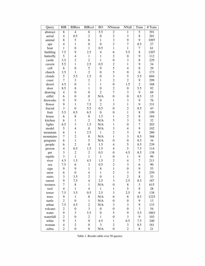
The results from these experiments are given in table 1.

The first column gives the query being searched for, the sec-

ond column is the number of images out of the nine images

returned by our algorithm which were labelled by the hu-

man subjects as being relevant to the query (precision × 9).

The third and fourth columns give the same kind of score

for our system, but restricting the features used to texture

only and color only, respectively. The fifth column shows

the results of the Behold online system, where N/A entries

correspond to queries which were not in the Behold vocab-

ulary. The sixth and seventh columns give the results for the

nearest neighbor algorithms using all members of the query

set and the mean of the query set respectively. The eighth

column gives the number of images out of the 9 randomly

displayed training images that were labelled by our subjects

as being relevant to the query. This gives an indication of

the quality of the labelling in the Corel data. The last col-

umn shows the number of training images, n, which com-

prise the query set (i.e. they were labelled with the query

word in the labellings which come with the Corel data).

Looking at the table we can notice that our algorithm us-

ing all features (BIR) performs better than either the texture

features (BIRtex) or color features alone (BIRcol); the p-

values for a Binomial test for texture or color features alone

performing better than all features are less than 0.0001 in

both cases. In fact our algorithm can do reasonably well

even when there are no correct retrievals using either color

or texture features alone (see, for example, the query “eif-

fel”). Our algorithm also substantially outperforms all three

of the comparison algorithms (BO, NNmean, NNall). It

tends to perform better on examples where there is more

training data, although it does not always need a large

amount of training data to get good retrieval results; in part

this may result from the particular features we are using.

Also, there are queries (for example, “desert”) for which

the results of our algorithm are judged by our two human

subjects to be better than a selection of the images it is train-

ing on. This suggests both that the original labels for these

images could be improved, and that our algorithm is quite

robust to outliers and poor image examples. Lastly, our al-

gorithm finds at least 1, and generally many more, appro-

priate images, in the nine retrieved images, on all of the 50

queries.

The average number of images returned, across all 50

queries, which were labelled by our subjects as belonging

to that query category, are given in figure 1. The error bars

show the standard error about the mean. Some sample im-

ages retrieved by our algorithm are shown in figures 4-7,

where the queries are specified in the figure captions.

By looking at these examples we can see where the al-

gorithm performs well, and what the algorithm mistakenly

assigns to a particular query when it does not do well. For

example, when looking for “building” the algorithm occa-

sionally finds a large vertical outdoor structure which is not

a building. This gives us a sense of what features the al-

gorithm is paying attention to, and how we might be able

to improve performance through better features, more train-

ing examples, and better labelling of the training data. We

also find that images which are prototypical of a particu-

lar query category tend to get high scores (for example, the

query “sign” returns very prototypical sign images).

We also compute precision-recall curves for our algo-

rithm and both nearest neighbor variants that we compared

to (figure 2). For the precision-recall curves we use the

labellings which come with the Corel data. Both nearest

neighbor algorithms perform significantly worse than our

method. NNall has a higher precision than our algorithm

at the lowest level of recall. This is because there is often

at least one image in the Corel test set which is basically

identical to one of the training images (a common criticism

BIR BIRtex BIRcol BO NNall NNmean Train 0

10

20

30

40

50

60

70

80

90

Pre

cis

ion

(%

)

Figure 1. mean ± s.e. % correct retrievals over 50 queries

0 0.2 0.4 0.6 0.8 10

0.2

0.4

0.6

0.8

1

Recall

Pre

cis

ion

BIR

NNmean

NNall

Figure 2. Precision-recall curves for our method (blue) and

both nearest neighbor comparison methods, averaged over all 50

queries, and using the Corel data labellings

of this particular data set). The precision of NNall imme-

diately falls because there are few identical images for any

one query, and generalization is poor. Our algorithm does

not preferentially return these identical images (nor does

NNmean), and they are usually not present in the top 9 re-

trieved.

Four sets of retrieved images (all features, texture only,

color only, and training) for all 50 queries can be found in

additional materials 1, which we encourage the reader to

have a look through.

4. Related Work

There is a great deal of literature on content-based image

retrieval. An oft cited early system developed by IBM was

“Query by Image Content” (QBIC [6]). A thorough review

1http://www.gatsby.ucl.ac.uk/˜heller/BIRadd.pdf

of the state of the art until 2000 can be found in [7].

We limit our discussion of related work to (1) CBIR

methods that make use of an explicitly probabilistic or

Bayesian approach, (2) CBIR methods that use sets of im-

ages in the context of relevance feedback, and (3) CBIR

methods that are based on queries consisting of sets of im-

ages.

Vasconcelos and Lippman have a significant body of

work developing a probabilistic approach to content-based

image retrieval (e.g. [8]). They approach the problem from

the framework of classification, and use a probabilistic

model of the features in each class to find the maximum a

posteriori class label. In [9] the feature distribution in each

class is modelled using a Gaussian mixture projected down

to a low dimensional space to avoid dimensionality prob-

lems. The model parameters are fit using EM for maximum

likelihood estimation. Our approach differs in several re-

spects. Firstly, we employ a fully Bayesian approach which

involves treating parameters as unknown and marginaliz-

ing them out. Second, we use a simpler binarized feature

model where this integral is analytic and no iterative fitting

is required. Moreover, we represent each image by a single

feature vector, rather than a set of query vectors. Finally,

we solve a different problem in that our system starts with

a text query and retrieves images from an unlabelled data

set—the fact that the training images are given a large num-

ber of non-mutually exclusive annotations suggests that the

classification paradigm is not appropriate for our problem.

PicHunter [10] is a Bayesian approach for handling rele-

vance feedback in content based image retrieval. It models

the uncertainty in the users’ goal as a probability distribu-

tion over goals and uses this to optimally select the next set

of images for presentation.

PicHunter uses a weighted pairwise distance measure to

model the similarity between images, with weights chosen

by maximum likelihood. This is quite different from our ap-

proach which models the joint distribution of sets of images

averaging over model parameters.

Rui et al [11] explore using the tf-idf2 representation

from document information retrieval in the context of im-

age retrieval. They combine this representation with a rele-

vance feedback method which reweights the terms based on

the feedback and report results on a dataset of textures. It

is possible to relate tf-idf to the feature weightings obtained

from probablistic models but this relation is not strong.

Yavlinsky et al [12] describe a system for both retrieval

and annotation of images. This system is based on modeling

p(x|w) where x are image features and w is some word

from the annotation vocabulary. This density is modeled

using a non-parameteric kernel density estimator, where the

kernel uses the Earth Mover’s Distance (EMD). Bayes rule

is used to get p(w|x) for annotation.

2term-frequency inverse-document-frequency

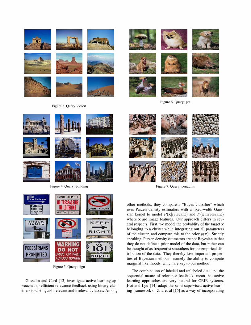
Figure 3. Query: desert

Figure 4. Query: building

Figure 5. Query: sign

Gosselin and Cord [13] investigate active learning ap-

proaches to efficient relevance feedback using binary clas-

sifiers to distinguish relevant and irrelevant classes. Among

Figure 6. Query: pet

Figure 7. Query: penguins

other methods, they compare a “Bayes classifier” which

uses Parzen density estimators with a fixed-width Gaus-

sian kernel to model P (x|relevant) and P (x|irrelevant)where x are image features. Our approach differs in sev-

eral respects. First, we model the probablity of the target x

belonging to a cluster while integrating out all parameters

of the cluster, and compare this to the prior p(x). Strictly

speaking, Parzen density estimators are not Bayesian in that

they do not define a prior model of the data, but rather can

be thought of as frequentist smoothers for the empirical dis-

tribution of the data. They thereby lose important proper-

ties of Bayesian methods—namely the ability to compute

marginal likelihoods, which are key to our method.

The combination of labeled and unlabeled data and the

sequential nature of relevance feedback, mean that active

learning approaches are very natural for CBIR systems.

Hoi and Lyu [14] adapt the semi-supervised active learn-

ing framework of Zhu et al [15] as a way of incorporating

relevance feedback in image retrieval.

In [16], the user manually specifies a query consisting of

a set of positive and negative example images. The system

then finds images which minimize the distance in color his-

togram space to the positive examples, while maximizing

distance to the negative examples. While our method is not

directly based on querying by examples, since it uses text

input to extract images from a labelled set, it implicitly also

uses a set of images as the query. However, in our system

the set only contains positive examples, the user only has

to type in some text to index this set, and the subsequent

retrieval is based on different principles.

5. Conclusions and Future Work

We have described a new Bayesian framework for

content-based image retrieval. We show the advantages of

using a set of images to perform retrieval instead of a sin-

gle image or plain text. We obtain good results from using

a Bayesian criterion, based on marginal likelihoods, to find

images most likely to belong to a query category. We also

show that this criterion can be easily and efficiently com-

puted as a matrix-vector multiplication when image feature

vectors are sparse and binary.

In all of our experiments, the two free parameters, the

preprocessing percentile threshold for binarizing the feature

vectors and κ, the scaling factor for setting the hyperparam-

eters, are set to 20 and 2 respectively. In our experience, this

initial choice of values seemed to work well, but it would be

interesting to see how performance varies as we adjust the

values of these two parameters.

In the future there are many extensions which we would

like to explore. We plan to extend the system to incorporate

multiple word queries where the query sets from all words

in the query are combined by either taking the union or the

intersection. We would also like to look into incorporating

relevance feedback, developing revised query sets, in our

Bayesian CBIR system. By combining with relevance feed-

back, the principles used here can also be applied to other

types of seaches, such as searching for a specific target im-

age. Lastly, we would like to explore using our Bayesian

CBIR framework to perform automatic image annotation as

well as retrieval.

Acknowledgements: Thanks to Alexei Yavlinsky for help

with the dataset and feature extraction. ZG was supported

partly by the DARPA CALO project at CMU.

References

[1] H. Tamura, S. Mori, and T. Yamawaki. Textual features cor-

responding to visual perception. IEEE Trans on Systems,

Man and Cybernetics, 8:460–472, 1978.

[2] P. Howarth and S. Ruger. Evaluation of texture features for

content-based image retrieval. In International Conference

on Image and Video Retrieval (CIVR), 2004.

[3] D. Heesch, M. Pickering, S. Ruger, and A. Yavclinsky. Video

retrieval with a browsing framework using key frames. In

Proceedings of TRECVID, 2003.

[4] Z. Ghahramani and K. A. Heller. Bayesian sets. In Advances

in Neural Information Processing Systems, volume 18, 2005.

[5] J. Bernardo and A. Smith. Bayesian Theory. Wiley, 2000.

[6] M. Flickner, H. Sawhney, W. Niblack, J. Ashley, Q. Huang,

B. Dom, M. Gorkani, J. Hafner, D. Lee, D. Petkovic,

D. Steele, and P.Yanker. Query by image and video content:

the qbic system. IEEE Computer, 28:23–32, 1995.

[7] A. W. M. Smeulders, M. Worring, S. Santini, A. Gupta, and

R. Jain. Content-based image retrieval at the end of the early

years. IEEE Transactions on Pattern Analysis and Machine

Intelligence, 22(12), 2000.

[8] N. Vasconcelos and A. Lippman. A bayesian framework for

content-based indexing and retrieval. In Proceedings of IEEE

Data Compression Conference, 1998.

[9] N. Vasconcelos. Minimum probability of error image re-

trieval. IEEE Transactions on Signal Processing, 52(8),

2004.

[10] I. Cox, M. Miller, T. Minka, T. Papathornas, and P. Yianilos.

The bayesian image retrieval system, pichunter: Theory, im-

plementation, and psychophysical experiments. IEEE Tran.

On Image Processing, 9:20–37, 2000.

[11] Y. Rui, T. Huang, and S. Mehrotra. Content-Based image re-

trieval with relevance feedback in MARS. In Proceedings of

IEEE International Conference on Image Processing, pages

815–818, 1997.

[12] A Yavlinsky, E Schofield, and S Ruger. Automated image

annotation using global features and robust nonparametric

density estimation. In Proceedings of the International Con-

ference on Image and Video Retrieval, 2005.

[13] P. H. Gosselin and M. Cord. A comparison of active classifi-

cation methods for content-based image retrieval. In First In-

ternational Workshop on Computer Vision meets Databases

(CVDB 2004), 2004.

[14] S. C. H. Hoi and M. R. Lyu. A semi-supervised active learn-

ing framework for image retrieval. In Proceedings of IEEE

Computer Society Conference on Computer Vision and Pat-

tern Recognition (CVPR 2005), 2005.

[15] X. Zhu, J. Lafferty, and Z. Ghahramani. Combining ac-

tive learning and semi-supervised learning using gaussian

fields and harmonic functions. In Proceedings of the ICML-

2003 Workshop on the Continuum from Labeled to Unla-

beled Data, 2003.

[16] J. Assfalg, A. Del Bimbo, and P. Pala. Using multiple ex-

amples for content-based image retrieval. In Proceedings of

the IEEE International Conference on Multimedia and Expo

(ICME 2000), 2000.

[17] Behold Image Search. Multimedia and Informa-

tion Systems Group, Imperial College London.

http://grouse.doc.ic.ac.uk:8800/searchvis.jsp

Query BIR BIRtex BIRcol BO NNmean NNall Train # Train

abstract 8 4 8 5.5 2 1 5 391

aerial 4 0.5 2 0 2 3 8 201

animal 8 5 6 1 3 9 9 1097

ape 4 1 0 0 2 7 8.5 27

boat 1 0 1 0.5 1 1 7 61

building 7.5 9 2.5 4 6 5.5 8 1207

butterfly 5 4 1 1 2 0 9 112

castle 3.5 2 2 1 0 3 8 229

cavern 5.5 1 2.5 0.5 2 1 9 34

cell 6 0 5 9 5 4 8 29

church 3.5 1 2 0 5 0 6 173

clouds 5 5.5 1.5 0 3 5 5.5 604

coast 7 3 2 1 2 2 9 299

desert 4.5 0 1 1 0 1.5 2 168

door 8.5 8 1 0 2 0 5.5 92

drawing 4 0 0 2 7 3 9 69

eiffel 6 0 0 N/A 0 0 8.5 15

fireworks 9 9 3 0 1 3 9 76

flower 9 1 7.5 2 3 1 9 331

fractal 3 0 5.5 0.5 0 2 8.5 43

fruit 5.5 0.5 6.5 0 0 1 8 199

house 6 8 0 1.5 1 2 8 184

kitchen 6 1 2 N/A 5 3 9 32

lights 6.5 3 1.5 N/A 1 0 7 203

model 5 4 0 N/A 3 4 9 102

mountain 6 1 2.5 1 2 3 8 280

mountains 7 2 8 N/A 1 3 8.5 368

penguins 6 1 5 N/A 0 0 8.5 34

people 6 2 0 1.5 4 5 8.5 239

person 4 0.5 1.5 1.5 4 5 7.5 114

pet 3 2 2 0.5 0 4.5 8.5 138

reptile 3 1 1 1 0 1 9 99

river 4.5 1.5 4.5 1.5 2 4 7 211

sea 7.5 6 3 0.5 2 3 6 90

sign 9 9 1 8 1 0 9 53

snow 6 0 4 1 2 3 9 259

stairs 3 3.5 2 0 1 2 8 53

sunset 9 7.5 4 2.5 3 2.5 8.5 187

textures 7 8 1 N/A 0 8 3 615

tool 4 1 4 1 1 5 9 28

tower 7.5 3.5 0.5 2.5 3 2.5 6 138

trees 9 1 8 N/A 6 8 8.5 1225

turtle 2 0 1 N/A 0 0 9 13

urban 7.5 4.5 2 N/A 3 3 9 133

volcano 2 0 3 0 0 0 3 54

water 9 3 5.5 0 5 9 5.5 1863

waterfall 2 0 2 1 0 3 9 103

white 9 3 9 4.5 1 6.5 7.5 240

woman 4 2 0 3 2 3 8.5 181

zebra 2 0 0 N/A 0 2 8 21

Table 1. Results table over 50 queries