A SIMTE

MPLE TEMPER

TEST PRATURE

ROCEDE CRAC

DURE FCK RES

United

for

FOR EVSISTANC

Ohio DepOffice of R

States DepFeder

Sta

r Transport

VALUATCE OF

CO

partment ofesearch an

partment ofral Highway

ate Job Num

N

Ohio Reation and th

TING LOASPHA

ONCRESang-SooShad SargAndrew W

fof Transporta

nd Developm

andf Transportay Administra

mber 13426

November 2

esearch Insthe Environm

OW ALT ETE o Kim gand

Wargo

or the ation ment

d the ation ation

60(0)

2009

titute ment

1. Report No. FHWA/OH-2009/5

2. Government Accession No.

3. Recipient’s Catalog No.

4. Title and Subtitle A Simple Test Procedure for Evaluating Low Temperature Crack

Resistance of Asphalt Concrete

5. Report Date November 2009 6. Performing Organization Code

7. Author(s) Sang-Soo Kim Shad Sargand Andrew Wargo

8. Performing Organization Report No.

9. Performing Organization Name and Address Ohio Research Institute for Transportation and the Environment 141 Stocker Center Ohio University Athens OH 45701

10. Work Unit No. (TRAIS)

11. Contract or Grant No. 134260

12. Sponsoring Agency Name and Address Ohio Department of Transportation

1980 West Broad St.

Columbus OH 43223

13. Type of Report and Period Covered Final Report

14. Sponsoring Agency Code

15. Supplementary Notes Prepared in cooperation with the Ohio Department of Transportation (ODOT) and the U.S. Department of Transportation, Federal Highway Administration 16. Abstract

The current means of evaluating the low temperature cracking resistance of HMA relies on extensive test methods that require assumptions about material behaviors and the use of complicated loading equipment. The purpose of this study was to develop and validate a simple test method to directly measure the cracking resistance of hot mix asphalt under field-like conditions.

A ring shape asphalt concrete cracking device (ACCD) was developed. ACCD utilizes the low thermal expansion coefficient of Invar steel to induce tensile stresses in a HMA sample as temperature is lowered. The results of the tests of the notched ring shaped specimens compacted around an ACCD Invar ring showed good repeatability with less than 1.0°C (1.8°F) standard deviation in cracking temperature. A laboratory validation indicated that ACCD results of five mixes correlate well with thermal stress restrained specimen test (TSRST) results with the coefficient of determination , r2 = 0.86. To prepare a sample and complete TSRST measurement, it takes minimum 2-3 days. For ACCD, two samples can be easily prepared and tested in a single day with a small test set-up. The capacity of ACCD can be increased easily with minimal cost to accommodate a larger number of samples.

Among factors affecting the low temperature performance of HMA, the coefficient of thermal expansion (CTE) of aggregate has been overlooked for years. A composite model of HMA is proposed to describe the low temperature cracking phenomenon. Due to the orthotropic and composite nature of asphalt pavement contraction during cooling, the effects of aggregate CTE is amplified up to 18 times for a typical HMA. Of 14 Ohio aggregates studied, the maximum and the minimum CTEs are 11.4 and 4.0 x 10-6/°C, respectively. During cooling, the contraction of Ohio aggregate with high CTE can double the thermal strain of asphalt binders in the asphalt mix and may cause asphalt pavement thermal cracking at warmer temperature.

17. Key Words Low Temperature Cracking, Asphalt Pavement, Coefficient of Thermal Expansion

18. Distribution Statement No Restrictions. This document is available to the public through the National Technical Information Service, Springfield, Virginia 22161

19. Security Classif. (of this report) Unclassified

20. Security Classif. (of this page) Unclassified

21. No. of Pages 118

22. Price

Form DOT F 1700.7 (8-72) Reproduction of complete pages authorized

A SIMPLE TEST PROCEDURE FOR EVALUATING LOW TEMPERATURE CRACK RESISTANCE OF ASPHALT

CONCRETE

Prepared in cooperation with the Ohio Department of Transportation

and the U.S. Department of Transportation, Federal Highway Administration

Prepared by

Sang-Soo Kim Shad Sargand

Andrew Wargo

Ohio Research Institute for Transportation and the Environment Russ College of Engineering and Technology

Ohio University Athens, Ohio 45701-2979

The contents of this report reflect the views of the authors who are responsible for the facts and the accuracy of the data presented herein. The contents do not necessarily reflect the official views or policies of the Ohio Department of Transportation or the Federal Highway Administration. This report does not constitute a standard, specification or regulation.

Final Report November 2009

iv

Acknowledgements

This projected was funded by the Ohio Department of Transportation (State Job Number 134260). The aggregates and asphalt mixes used in this study were collected with help from Mr. David Powers of ODOT at the Central Laboratory and many engineers and staff at ODOT District Offices. Recycled asphalt pavement (RAP) mixes were provided by Mr. Clifford Ursich of Flexible Pavement of Ohio with help from Kokosing Construction Company Inc. Their support for this research is gratefully acknowledged.

v

TABLE OF CONTENTS

page Abstract Acknowledgments List of Tables List of Figures 1. Introduction 1 1.1 Statement of Problem 1 1.2 Objectives of Study 2 2. Literature Review 3 2.1 Asphalt Binder Properties 3 2.1.1 Asphalt Binder Rheology and Temperature

Susceptibility 3

2.1.2 Glass Transition and Low Temperature Physical Hardening

4

2.1.3 Binder Effects on Low Temperature Cracking 5 2.1.4 Modification of Binders 6 2.2 Mix Properties 8 2.2.1 Effects of Aggregate Properties 8 2.2.2 Effects of Other Mix Properties 9 2.3 Climatic, Age Hardening and Traffic Effects 9 2.3.1 Minimum Temperature 10 2.3.2 Rate of Cooling 10 2.3.3 Traffic Effects 11 2.3.4 Aging Effects 11 2.4 Pavement Structure 13 2.5 Evaluating the Low Temperature Behavior of Asphalt

Concrete 14

2.5.1 Finite Element Analysis 14 2.5.2 Binder Tests 14 2.5.3 Asphalt Binder Cracking Device 17 2.5.4 Mixture Testing 17 2.6 Fixed Frame Restrained Cooling Tests 20 3. Coefficient of Thermal Expansion (CTE) of Ohio Aggregates 22

vi

3.1 Determination of Aggregate CTE using Strain Gage Technique

22

3.2 Significance of Aggregate CTE in HMA Low Temperature

Cracking 25

3.3 CTE of Asphalt Mixes 26 4. Fixed Frame with an Epoxied Cylindrical Sample 36 4.1 Summary of the Test Procedure 37 4.2 Fixed Frame Test Results 40 4.3 Areas of Concern With the Test Method 42 4.3.1 Sample Geometry 42 4.3.2 Epoxying 43 4.3.3 Alignment 43 4.3.4 Apparatus Problems 44 4.3.5 Test Problems 44 4.4 Benefits of the Test Method 45 5. Concentric Ring ACCD Apparatus 46 5.1 Design of the Apparatus 47 5.1.1 Long Mold ACCD (Variation 1) 49 5.1.2 Short Mold ACCD (Variation 2) 50 5.2 Development of the Test Method 51 5.3 Effects of Length of Notch on Cracking Temperature 53 5.4 Finalized ACCD Test Procedure and Determination of

Cracking Temperature 56

5.5 Repeatability of Concentric ACCD Ring Test 59 5.6 Validation of ACCD 63 5.6.1 Correlation between ACCD and TSRST 64 5.6.2 Correlation between ACCD and Bending Beam

Rheometer (BBR) 68

5.6.3 Correlation between ACCD and Asphalt Binder Cracking Device (ABCD)

69

5.7 ACCD Results of Ohio DOT Mixes 70

vii

5.8 Effects of Variations in ACCD sample Geometry 72 6. Finite Element Analysis 74 6.1 Cylindrical Sample Epoxied to a Fixed Frame 74 6.2 Concentric Ring Apparatus 77 7. Conclusions and Recommendations 83 7.1 Conclusions 83 7.2 Recommendations for Further Research 84 8. References 85 Appendix A 90 Developmental History and Test Procedure of the Fixed Frame Test Appendix B 95 Standard Procedure for the Concentric Ring ACCD Test Appendix C 99 Materials Used Appendix D Implementation Plan 105

viii

LIST OF TABLES

page

Table 3.1 Coefficient of Thermal Expansion of 14 Aggregates from 9 Ohio DOT Districts and 6 Aggregates from WRI Test Roads 24

Table 3.2 CTE of Asphalt Mixes Predicted Using the Composite Model and the Rule of Mix 31

Table 3.3 Sensitivity Analysis of Mix CTE Determined by Composite Model 32

Table 3.4 Effective Asphalt Binder CTE in HMA. 34

Table 4.1 Summary of Fixed Frame Test Results 41

Table 5.1 ACCD Results of RAP Mixes 61

Table 5.2 Average ACCD Results of RAP Mixes (38.1 mm or 1.5 in. Notch Length). 62

Table 5.3: Five SHRP Core Asphalt Used in ACCD Validation 65

Table 5.4 ACCD Results of SHRP Binder Mixes 66

Table 5.5 Average ACCD Results of SHRP Binder Mixes 67

Table 5.6 ACCD Results of ODOT Mixes 71

Table 5.7 Average ACCD Results of ODOT Mixes 71

Table 6.1 Stress Concentration Factors 81

ix

LIST OF FIGURES page

Figure 3.1 Strain gages instrumented on the polished aggregate surfaces 22

Figure 3.2 Temperature versus the corrected strain to determine aggregate CTE 23

Figure 3.3 Composite models; Hirsch model and Counto model 26

Figure 3.4 Idealized packing of aggregate and asphalt binder and 3-D cubic phase diagram 28

Figure 3.5 Poisson’s effect of asphalt binder coated on aggregate surface 30

Figure 4.1 The fixed frame test setup during alignment 38

Figure 4.2 The fixed frame setup ready to be tested 39

Figure 4.3 Typical test result for the fixed frame setup 39

Figure 4.4 Aggregate gradations used in the mixes for the fixed frame test 40

Figure 5.1 ACCD ring (at the center) with HMA compacted outside 46

Figure 5.2 Concentric ring ACCD long mold (variation 1) after compaction 48

Figure 5.3 ACCD concentric ring short mold (variation 2) after compaction 48

Figure 5.4 ACCD mold and pressing head 50

Figure 5.5 Readings from strain gages aligned and not aligned with the 38.1 mm (1.5 in.) notch 9 53

Figure 5.6 Effect of notch length on strain and cracking temperature 55

Figure 5.7 Effect of cross section length on cracking temperature (RAP samples) 55

Figure 5.8 Effect of cross section length on cracking temperature of AAA-1 and AAC-1 mixes 56

Figure 5.9 Example of graphical procedure for determining cracking temperature from well defined peak strength 58

Figure 5.10 Example of graphical procedure for determining cracking temperature from transitional failure 58

x

Figure 5.11 Strain versus temperature with mix 40% RAP 5% SBR 38.1 mm (1.5 in.) notch length (6 replicates) 59

Figure 5.12 Strain versus temperature with mix 40% RAP 0% SBR 38.1 mm (1.5 in.) notch length (6 replicates) 60

Figure 5.13 ACCD cracking temperature versus SBR content 62

Figure 5.14 Aggregate gradation for the SHRP core asphalt mixes 65

Figure 5.15 ACCD versus TSRST cracking temperatures for SHRP binders 67

Figure 5.16 ACCD cracking temperature versus BBR critical temperature for SHRP binders 68

Figure 5.17 ACCD versus ABCD cracking temperatures (SHRP core asphalt mixes) 69

Figure 5.18 ACCD cracking temperature versus BBR critical temperature (ODOT mixes) 72

Figure 5.19 ACCD cracking temperature versus fracture area (ODOT samples) 73

Figure 6.1 Assumed behavior model for fixed frame test 76

Figure 6.2 Maximum principal stresses for the fixed frame setup (MPa) 76

Figure 6.3 Assumed stress distribution in the HMA sample and Invar ring 78

Figure 6.4 Model used for finite element analysis 78

Figure 6.5 Max principal stresses in the concentric ring setup (57.2 mm or 2.25 in. notch) (MPa) 79

Figure 6.6 Max principal stresses for the concentric ring setup (50.8 mm or 2.0 in. notch) (MPa) 79

Figure 6.7 Max principal stresses for the concentric ring setup (38.1 mm or 1.5 in. notch) (MPa) 80

Figure 6.8 Max principal stresses for the concentric ring setup (25.4 mm or 1.0 in. notch) (MPa) 80

Figure 6.9 Max principal stresses for the concentric ring device (no notch) (MPa) 81

1

1. INTRODUCTION

1.1 Statement of Problem

Low temperature cracking is one of the major distress modes in asphalt pavement. The

low-temperature cracks are non-load associated, occur in the transverse direction of the

pavement, and are typically evenly spaced. As the ambient air temperature drops, asphalt

mixtures shrink due to thermal contraction. The pavement also stiffens and becomes brittle.

Thermal stress is induced in the asphalt mixture since the friction between the pavement and

underlying pavement structure resists the asphalt from contraction. When the thermal stress

exceeds the tensile strength of the asphalt pavement, a transverse crack will develop at the

surface to relieve the stress. This non-load associated crack can occur from a single critically

low temperature or from a thermal cycle that fluctuates just above the critical cracking

temperature. Jung and Vinson (1994) reported that at colder temperatures or repeated

temperature cycles, the crack will penetrate the full depth and width of the asphalt mixture layer.

The crack initiates at the surface because it is cooled first. Thermal stresses are generally equal

throughout the length of a road with a constant air temperature; thus, the cracks tend to be evenly

spaced.

These asphalt concrete failures caused by low-temperature cracking are disastrous to

pavement performance and service life. A poor riding surface leads to an increase in

maintenance and eventual early replacement of the pavement. When overlaid, these cracks

reflect through the new pavement. This costs taxpayers more money and time waiting for road

construction. Therefore, it is imperative to know the critical cracking temperature of a mixture

proposed for new construction in order to prevent or prolong the aforementioned failures.

Mix variables, such as asphalt binder grade, asphalt content, aggregate type and gradation, and

additives including polymers, affect the thermal properties, rheological properties and tensile

strength of asphalt mixes, consequently affecting low temperature cracking potential for a given

environment. Currently, there are two approaches to characterize the low temperature thermal

cracking potential of asphalt concretes; (1) mechanistic-empirical analysis (Superpave Indirect

Tensile Creep and Strength Test, IDT) and performance model and (2) a torture test (Thermal

Stress Restrained Specimen Test, TSRST). Both methods have been validated with field

2

performance data and predict the low temperature cracking potential of asphalt concrete mixes

well. However, neither test can be readily used as a routine test because of the complex test and

analysis procedures for IDT and the costly specialized equipment, and the difficulty producing

beam specimens for TSRST. Furthermore, with the current test methods, determination of the

cracking potential of asphalt mixtures caused by thermal fatigue is practically impossible. Many

states in the US including Ohio suffer with a high number of warm/cold cycling and occasional

severe freezing. A new simple test procedure is needed to evaluate the low temperature cracking

potential for a single severe freezing event and thermal fatigue for the environment and materials

commonly used in Ohio.

1.2 Objectives of Study

This study has four main objectives:

To determine coefficient of thermal expansion of Ohio aggregates and mixes,

To develop a simple test procedure, as a part of a mix design system, to determine the

thermal cracking resistance of asphalt concrete mixes,

To validate the simple test device by laboratory testing, and

To determine the thermal cracking resistance of typical ODOT asphalt concrete mixes

prepared with local materials for the future validation of the new test device.

In this report, a comprehensive literature review is presented in order to identify previous work

in this area, to provide a summary of the factors that affect the low temperate behavior of HMA,

as well as to obtain data with which to compare the results of this study. For the developed test

methods, the results from validation experiments are presented in order to facilitate further

research using these test methods. Finally, the developed test setups are evaluated using finite

element modeling to better understand the stress distributions during the test.

3

2. LITERATURE REVIEW

A literature review was performed to understand the current body of knowledge

pertaining to the low temperature cracking of HMA pavements. This phenomenon is highly

complex and influenced by many factors. These factors were summarized by Haas and Phang

(1988):

1. Climatic effects

2. Asphalt binder properties

3. Mix design/properties

4. Pavement design (including subgrade).

5. Construction flaws

6. Pavement age and traffic effects

For purposes of clarity and ease of explanation, most of these factors will be discussed in

more detail in subsequent sections of this report. Following these sections, a detailed description

of the test methods developed for the evaluation of the low temperature performance of HMA

mixtures will be presented.

2.1 Asphalt Binder Properties

It is generally recognized in the HMA industry that the low temperature performance of

HMA is controlled mostly by binder properties (Isacsson & Zeng, 1998). Low temperature

cracking is caused by excessive tensile stresses within the HMA layer when the pavement

temperature is lowered. Since asphalt binder is the material responsible for giving a mixture its

tensile strength, binder type is the primary factor in determining a mixture’s resistance to tensile

failure at low temperature. In order to understand its effect on pavement performance, one must

understand the nature of asphalt binders.

2.1.1 Asphalt Binder Rheology and Temperature Susceptibility

Asphalt binders are visco-elastic materials. This means that their response to a given load

will be a combination of both elastic and viscous behavior. This behavior is dependant on the

4

temperature. At high temperatures asphalt binder is nearly a viscous fluid. Thus, as a load is

applied, the binder experiences a near constant deformation for the duration of the load. These

deformations are not recovered when the load is removed. At cold temperatures, asphalt behaves

like a perfectly elastic glassy solid. Thus, as a load is applied, elastic strains develop in the binder.

These strains are recovered immediately after the load is released. At intermediate temperatures,

the behavior becomes more complex: the response is a combination of both elastic and viscous

responses. Like temperature, the time of loading also plays a large role in a binder’s response to

an applied load. Under short loading times, an asphalt binder at an intermediate temperature may

behave entirely elastically. Conversely, at long loading times at the same temperature it may

behave like a slow moving liquid. While all asphalt binders have the same general behavior, each

binder exhibits a different stiffness at a given temperature and loading time. At a certain

temperature, one asphalt may be soft and ductile while another is hard and brittle. Furthermore,

equalities in the stiffness of different asphalt binders at a single temperature and loading time

does not mean that the asphalts are the same. For example, two asphalts with equal stiffness at

40°C may have drastically different stiffness from each other at 0°C. This is due to the fact that

as the temperature changes, some binders show large changes in stiffness while others show

small changes in stiffness. This is known as temperature susceptibility. Asphalts with a larger

change in stiffness due to a change in temperature are said to have high temperature

susceptibility. In general, asphalts with higher temperature susceptibility are unable to relieve

stresses as easily at low temperatures and thus experience more thermal cracking than less

temperature susceptible asphalts.

2.1.2 Glass Transition and Low Temperature Physical Hardening

At low temperatures, asphalt begins another change in properties. Due to a decrease in

molecular mobility at these temperatures, the binder behaves more like a brittle solid than a

visco-elastic material. This transition is not an abrupt change but rather takes place over a range

of temperature. This type of behavior is known as the glass transition (Young, Mindess, Bentur,

& Gray, 1998). For some asphalts, this temperature range is wide. Once a binder enters its glassy

state, the dissipation of applied loads is essentially eliminated and failure is brittle in nature.

Thus, binders with higher glass transition temperatures will be less able to resist low temperature

cracking. It has been shown by previous researchers that the glass transition behavior varies

5

significantly between binders and is dependent on the rate of change in temperature (Bahia &

Anderson, 1993). A similar effect to the glass transition is physical hardening. It was discovered

that asphalts and polymers that were stored at low temperatures for long periods of time were

stiffer than those tested after minimal time at low temperatures. Much like the glass transition,

this phenomenon is due to the rearrangement of the complex molecules in asphalt binder. If

cooled sufficiently quickly, these molecules do not have time to move into their optimal low

energy arrangement (Johansson & Isacsson, 1998). Thus, with increased storage time at low

temperature, these molecules slowly realign themselves into a lower energy configuration. This

has the effect of increasing the stiffness of the material. It was found by Lu & Isacsson (2000)

that the rate of physical hardening is high at the beginning of isothermal storage and decreased

with time. Physical hardening can occur above or below the glass transition temperature of the

asphalt binder. This phenomenon is reversible if the material is heated to a high enough

temperature (Krishnan & Rajagopal, 2005).

The increased stiffness due to physical hardening means that a physically hardened

binder can dissipate less thermal stress through viscous flow, and thus has a higher potential for

cracking. However, while the existence of physical hardening in asphalt binders is easily

measurable, there is debate as to what effect this phenomenon has on the performance of asphalt

mixtures. The existence of the asphalt binder as a film between aggregate particles may prevent

physical hardening from occurring in asphalt concrete (Shenoy, 2002). Conversely, since binder

behavior is the dominant factor in the occurrence of low temperature cracking and physical

hardening has a significant effect on the binder stiffness, some believe that physical hardening is

likely an important phenomenon in mixes.

2.1.3 Binder Effects on Low Temperature Cracking

Low temperature cracking of HMA mixtures is caused by the buildup of thermal stresses

due to a drop in pavement temperature. As the pavement cools, it attempts to contract. However,

due to frictional restraint by the pavement substructure, it cannot. This induces tensile stresses in

the pavement layer along its length. At higher temperatures, with reasonable field cooling rates,

asphalt binders can relieve these thermal stresses by viscous flow. However, as temperatures

continue to fall, the viscous flow may not be fast enough to alleviate all of these stresses.

Consequently thermal stresses begin to build in the pavement. With even further temperature

6

decrease, the asphalt binder undergoes its glass transition and will behave more brittle with

continued temperature change. Eventually, the thermal stresses in the pavement exceed the

tensile strength of the pavement and a crack forms from the pavement surface downward

(Roberts et al. 1996).

2.1.4 Modification of Binders

From the failure mechanism described above, it is advantageous to use soft binder to

minimize low temperature cracking. However, using a binder that is too soft causes problems at

a high service temperature, such as rutting. Thus, pavement engineers are limited as to how soft

an asphalt can be. Producing binder that meets high temperature requirements and is soft enough

to produce good low temperature performance is challenging with conventional asphalt alone.

Minimizing temperature susceptibility is important in attempting to reduce this conflict between

high and low temperature properties. However, even binders with low temperature susceptibility

may not always have adequate rheological properties to relieve the induced thermal stresses at

low temperature. In areas that experience a wide range between high and low pavement

temperatures, it is often impossible to meet the specifications without some sort of modification.

Many additives and forms of modification have been attempted to improve low temperature

performance of asphalt binders. Some of the most important include polymer modification,

crumb rubber, and mineral fillers. Others are dewaxing, air blowing/air oxidation, metal-

complexes and inorganic catalysts, acid treatment, caustic washing, gelling agents, aldehyde/acid

reactions, oils and softening agents (King et al., 1999). The addition of polymer additives to

asphalt binder is the most common form of modification.

Polymer Modification

A polymer is a complex, long chain organic compound. There are two major groups of

polymers used for asphalt binder modification: elastomers and plastomers. Their names are

indicative of their behavior. Elastomers “can be stretched and elastically recover their shape

when released. Such polymers add only a little strength to the asphalt until they are stretched”.

Plastomers “form a tough, rigid, three dimensional network. These polymers give high early

strength to resist heavy loads, but may crack at higher strains” (King et al., 1999 p. 37).

7

All modified binders used in this study contained elastomers. Mixes containing both

Styrene Butadiene Rubber (SBR) and Styrene Butadiene Styrene (SBS) elastomers were used for

testing and validation purposes. SBR and SBS polymers contain the same chemical constituents

(known as mers), the only difference being that SBR is composed of individual mers reacted

randomly, while SBS has the mers arranged in a regular structured order. Due to this regular

structure SBS has a higher tensile strength than does SBR (King et al., 1999).

The main advantage of elastomers such as SBR and SBS is that they can help to provide

a higher strength when strain levels are high (King et al., 1999). Due to the visco-elastic nature

of asphalt binders, high strains are experienced at high temperatures. This means that asphalt

binders modified with elastomers will show increased strength at high temperatures. This

increased high temperature strength allows for the use of a softer base bitumen while still

meeting the high temperature specifications. As stated previously, a softer asphalt is better for

low temperature performance. Additionally, research has demonstrated other benefits of using

polymer modified binders. It was found by Stock and Arand (1993) that polymer modification

“always improves low temperature performance” of a binder (p. 45). This study found that

higher fracture stresses and lower fracture temperatures are characteristic of polymer modified

binders. Other research has also indicated that increased polymer content decreases cracking

temperature (King et al., 1993). Additional research has shown that elastomer addition can lower

the glass transition temperature and decrease the low temperature creep stiffness of asphalt

binders (Lu et al., 1998.) This is advantageous since decreasing these values tends to increase the

low temperature performance of the binder.

Other studies have discussed other mechanisms in polymer modified binders that may

enhance the low temperature properties of HMA pavements. At low temperatures, the addition of

polymer tends to arrest the propagation of cracks through the binder and alter the type of

cracking observed. One study suggested that the increased performance due to polymer addition

may be caused by the polymers helping to “blunt crack tips” and by the improvement of “the

bulk yield characteristics” of the HMA mix (Lee et al., 1995 p. 536). It was shown by Hesp et al.

(2000) using restrained cooling tests, that mixes containing polymer modified asphalts did not

show a clear catastrophic failure. It was proposed that the reason for this was the formation of

“multiple microcracks at the binder-aggregate interface that were prevented from becoming

catastrophic due to the increased toughness imparted by the SBS modifier” (p. 554.)

8

In summary, polymer modification not only has the benefits of increasing high

temperature performance, thus allowing for use of a softer base bitumen, but also may have the

effect of improving the resistance to low temperature crack formation. This makes polymer

modification extremely attractive for pavement designers and highway agencies.

2.2 Mix Properties

Although the asphalt binder is the major factor determining the low temperature

performance of HMA mixes, many other factors of mix design also have limited effects. It has

long been suggested that mixture tests be performed to better determine the low temperature

cracking resistance of a particular pavement rather than relying on binder tests alone (Goodrich,

1991). More recently, research has indicated that using binder properties alone will produce

unrealistic predictions of low temperature pavement performance (Bahia et al., 2000). The

factors causing this discrepancy can be generally factored into two groups: effects of aggregate

properties and effects of other mix properties, which are discussed in the following sections.

2.2.1 Effects of Aggregate Properties

The strength and the coefficient of thermal expansion (CTE) of aggregates might be two

most important properties affecting low temperature performance of HMA. On average, the

crushing strength of aggregates varies from about 210 MPa (30 x 103 psi) to 90 GPa (13 x 106

psi). There is also large variation within the same type of aggregate. The strength of 241

limestones in a study varied from 96 MPa (14,000 psi) to 240 MPa (35,000 psi). There is also a

significant variation in CTE of aggregates; about 5 x 10-6 per °C for limestones , 5 x 10-6 per °C

for granite, and 11 x 10-6 per °C for quartzite (Metha and Monterio, 2006).

However, there is no clear answer as to exactly what effect variation in aggregate has on

the low temperature mix properties. Some research has shown that the variation of aggregate

gradation has little effect on the tensile strength of HMA mixes at low temperature (Haas and

Phang, 1988). Others have found that aggregate type does not have a large impact on strain at

failure for the mixture (Johnson et al., 1979; Ruth et al., 1979). While this early research

indicated that aggregate has little effect on low temperature cracking, more recent studies have

found that aggregate type does have a limited effect on low temperature cracking. Using the

9

Thermal Stress Restrained Specimen Test (TSRST), Jung and Vinson (1993; 1994) found that

aggregate type is an important factor in the low temperature cracking resistance of HMA samples.

A more recent study by Marasteanu et al. (2007) confirmed this result. It was shown that mixes

containing granite aggregate performed slightly better in TSRST test than mixes containing

limestone aggregate. Both of these studies demonstrate that aggregate properties play a role in

the low temperature cracking resistance of HMA mixtures. Thus, basing low temperature

performance predictions on binder properties alone without considering aggregate effects would

not be completely accurate. Additionally, other mixture properties besides aggregate type

influence the low temperature behavior of HMA mixes. Two of these are described in the next

section.

2.2.2 Effects of Other Mix Properties

Mix properties such as thermal expansion coefficient and air voids also have an effect on

the low temperature performance of HMA mixes. The effects of mix thermal expansion are

obvious: the higher the thermal expansion coefficient the more thermal stress will develop for a

given temperature change. The effects of air voids are less obvious. In general, it is assumed that

lower air voids will produce better low temperature performance. It was found that using

restrained specimen tests (TSRST) mixes with 4% air voids had more resistance to low

temperature fracture than mixes with 7% air voids (Marasteanu et al., 2007). Other studies have

found that air voids influence the fracture strength of the mix (Jung and Vinson, 1993), lower air

voids correlated to higher failure strains within the mix (Masad et al., 2001) and that fracture

toughness increases with lower air void content (Marasteanuet al., 2002). Additionally, higher air

voids also have the effect of lowering the thermal expansion coefficient of the mix (Haas and

Phang, 1988).

2.3 Climatic, Age Hardening and Traffic Effects

The environmental conditions that a pavement must endure during its design life

determine its potential to experience thermal cracking. Climatic factors are outside the scope of

10

human control and must be designed for. Factors such as thermal fatigue and long periods of

cold, which may allow for physical hardening, may play a role in the development of low

temperature cracking (Bouldin et al., 2000). However, the most important climatic factors

effecting low temperature performance of HMA pavements are the minimum temperature and

the rate of cooling of the pavement. Also, constant exposure to traffic, oxygen, high temperatures

and sunlight damage HMA roadways and can increase their propensity to thermal cracking.

2.3.1 Minimum Temperature

The lowest temperature experienced by the pavement is directly related to the occurrence

of thermal cracking. A lower temperature will cause more thermal contraction and thus induce

greater thermal stresses in the pavement. For this reason colder areas have more problems with

thermal cracking than warmer ones. Thus, when attempting to mitigate low temperature

distresses while maintaining high temperature performance of the mix, the pavement designer

must accurately determine the extreme temperatures that the pavement will be subjected to. This

is not as easy as simply measuring air temperatures; many factors affect the pavement

temperature including ambient temperature, solar radiation, wind speed and reflectance of the

pavement surface (Diefenderfer et al., 2002). Thus, a climatic model, such as FHWA’s LTTP-

Bind software, calibrated for the regional effects of these parameters must be employed to

accurately predict the actual low pavement temperature expected at the site.

2.3.2 Rate of Cooling

The rate of cooling is also an important factor in low temperature cracking. As with

mechanical loading, faster thermal loading on a visco-elastic material allows less time for

stresses to be relieved and thus translates into more rapid stress buildup and rupture. Cooling

rates in the field generally range between 0.5-3°C/hr and are dependant on site location (Bouldin

et al., 2000). It was found that the rate of cooling has a noticeable effect on thermally restrained

lab specimens up until about 5°C/hr; at cooling rates higher than 5°C/hr little additional variation

is observed (Jung and Vinson, 1993; Chehab et al., 2004). Cooling rates of 10°C/hr are common

for laboratory research purposes in order to keep testing time relatively short.

11

2.3.3 Traffic Effects

The effects of traffic on low temperature cracking are not well known. Using

mathematical models, Marasteanuet al. (2004) studied the effects of the superposition of axle

loadings on a pavement at low temperature. This research showed that at low temperatures,

wheel loading induced small zones of tensile stresses at the top of the HMA layer. This tension

may help to initiate failure of the pavement at low temperature. When comparing these results

with field data, it was found that the driving lane, which had been exposed to more traffic,

exhibited more cracking than the passing lane. This study showed that the application of repeated

traffic loading increases the formation of low temperature cracks. Thus, damage from traffic

loadings combined with other effects, such as aging, can contribute to the early failure of a

pavement.

2.3.4 Aging Effects

Aging also plays a role in the decreased low temperature performance of field HMA

mixtures. Aging is the hardening of asphalt binder over time due to exposure to oxygen and other

environmental factors. Oxidation and volatilization are the most important factors in aging

(Isacsson and Zeng, 1997); these processes occur significantly faster at higher temperatures. In

the laboratory, aging can become a problem if samples are heated repeatedly or for long periods

of time; in the field, aging is an unavoidable reality, and is most severe during summer months.

Since stiffness is of major importance to the occurrence of low temperature cracking, aging must

be adequately understood and accounted for if any design is to be successful.

Types of Aging

There are generally two types of aging, short term and long term aging. Short term aging

is the hardening experienced in an HMA mixture as it is mixed, transported to the job site and

placed. During this time the mixture is subjected to oxygen and is kept at relatively high

temperatures. This means oxidation occurs and volatile compounds are released. This has the

effect of stiffening the asphalt binder. The second form of aging is long term stiffening over the

life of the pavement. This stiffening occurs as the pavement is subjected to oxygen, sunlight and

other environmental factors. Since stiffer pavements are less resistant to low temperature

12

cracking, determining what factors affect aging, how to mitigate them, and how to make lab

samples adequately approximate the properties of field samples are important.

Laboratory Simulation of Field Aging

For design purposes, laboratory prepared specimens need to closely approximate the

properties of field samples. This approximation is achieved in two ways: binder aging and

mixture aging. In order to simulate the aging of the asphalt binder, two standard procedures are

used: Rolling Thin Film Oven Test (RTFOT) (AASHTO T 240) and Pressure Aging Vessel

(PAV) procedure (AASHTO R 28). RTFOT simulates short term aging. This process involves

heating the binder to high temperatures and exposing it to oxygen at a specified rate. During this

process, the binder is oxidized and volatile compounds are released. After RTFO aging, the

binder is approximately as stiff as the asphalt binder in HMA pavements immediately after

construction. To simulate several years of in service life, the PAV procedure must be performed.

This device typically heats pans of binder up to 100°C and subjects them to an air pressure of

300 psi for 20 hours. These conditions accelerate the oxidation processes that occur slowly over

the lifetime of the pavement. However, this process cannot account for any other types of aging

that may occur, such as degradation by sunlight; thus, all stiffening occurs through oxidation.

While the RTFO and PAV are believed to adequately estimate the stiffening that occurs

during aging, they are still simplified laboratory techniques that approximate field phenomena;

thus, they cannot 100% accurately represent the aging of all mixes under field conditions. This

problem is especially true when considering the effects of mixture properties on the aging of the

asphalt binder within the mix. Additionally, aging is a problem when attempting to correlate the

performance of laboratory mixture samples and field mixture samples. Thus, aging procedures

have been developed for mixtures as well. To approximate aging, specimens are placed in an

oven for a certain period of time. This exposure to high temperature air allows them to oxidize

sufficiently to better approximate their field performance. To approximate short term aging,

loose samples are placed in an oven at a fairly high temperature for several hours before

compaction. To approximate long term aging, compacted samples are held at a slightly lower

temperature for several days.

Unlike binders, which are homogeneous substances, the aging of mixes is more

complicated. The volumetric and geometric properties of an HMA mix have a significant effect

13

on the field aging it experiences. One of these properties is percent of the total mix volume filled

with air (percent air voids). A higher percent air voids allows oxygen to more easily move

through the pavement structure; thus, as percent air voids increases, the amount of aging

increases (Isacsson and Zeng 1998). Similarly, as the asphalt layer thickness increases, less

oxygen is able to reach the lower layers; thus, the degree of aging changes with depth in a

pavement structure (Li et al., 2006). Since minimizing the pavement’s exposure to oxygen is

desirable, obtaining high field densities is important to reducing age hardening.

2.4 Pavement Structure

In addition to reducing the aging in lower layers, the design of the pavement structure has

other effects on the low temperature cracking performance of a roadway. Pavement thickness

and subgrade properties are of importance to the low temperature performance of asphalt

mixtures. It has been found that thicker pavements have less cracking, possibly due to reduced

effects of traffic induced damage (Iliuta et al., 2004).

Also, it was found using finite element analysis, that pavements experienced bending

effects due to the thermal gradient with respect to depth; these effects cause a slight increase in

tensile stresses at the top of the pavement layer. This slightly increased the occurrence of thermal

cracking (Marasteanu et al., 2004). This study concluded that thicker HMA layers suffer more

from the effects of thermal gradients than do thinner ones. Other findings of this study were that

increasing the internal friction in the subbase increased the occurrence of thermal cracking and

that higher frictional restraint meant a higher rate of stress increase with a temperature drop. By

comparing the cracking occurring at airports across Canada, Haas et al. (1987) determined that

base and subbase thicknesses appear to have limited effect on the overall occurrence of thermal

cracking.

This research illustrates that the effect of a pavement structure is complex and that the

results are often conflicting from study to study. Due to this complexity, it is virtually impossible

to simulate these factors in the laboratory. For this reason, most methods for determining low

temperature cracking resistance of pavements ignore these factors.

14

2.5 Evaluating the Low Temperature Behavior of Asphalt Concrete

Many methods have been proposed to predict the low temperature performance of HMA

pavements. These include empirical laboratory tests, mathematical models, and combinations of

both. Due to the complex nature of the problem, all of these approaches have met with varying

degrees of success. The next sections will discuss the key methods for evaluating the low

temperature performance of HMA in detail.

2.5.1 Finite Element Analysis

As reviewed in the previous sections, many factors affect the low temperature pavement

cracking. To accurately simulate all of these factors in the laboratory is impossible. Finite

element models can be used for this purpose. However, the success of any mathematical model is

dependent on the accuracy of its assumptions and the quality of its input. Work by Marasteanu et

al. (2004) is a good example of this. In this study, three levels of analysis were used, each with a

certain degree of accuracy and required inputs. The simplest level required few inputs which are

easy to obtain and thus was easy to perform and utilize. However, if the default values make too

many unwarranted or inaccurate assumptions, the accuracy of the predictions of pavement

performance is questionable. Conversely, the highest level of analysis contained a very

complicated model. While very comprehensive, this model required many inputs that were

difficult to obtain. Due to this complexity, this model was not practical as a routine analysis.

Thus, while complex mathematical models are useful tools for evaluation of pavement

performance, they are limited by their inputs and assumptions. Often these models require

extensive laboratory testing to determine important physical properties of the mix. Thus, such

analysis is not typically done when designing a pavement for low temperature cracking

resistance.

2.5.2 Binder Tests.

Rather than implementing a comprehensive model accounting for every material behavior,

it is far easier to utilize a simpler mathematical model combined with a laboratory test to help to

predict performance at low temperature. As noted previously, binder properties dominate the

performance of HMA mixtures at low temperature (Isacsson and Zeng, 1998). For this, binder

15

tests have long been performed in an attempt to design better performing pavements. Originally,

there were many types of empirical tests that attempted to grade asphalt binders with respect to

their performance. Many of these were not accurate. A test method that would closely simulate

field failure mechanisms and would provide a better indication of field performance was needed.

One of the goals of the Strategic Highway Research Program (SHRP) was to develop such a test.

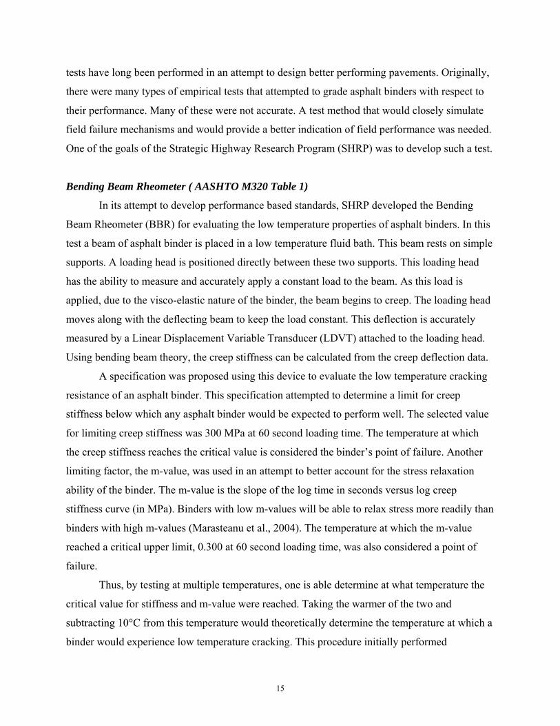
Bending Beam Rheometer ( AASHTO M320 Table 1)

In its attempt to develop performance based standards, SHRP developed the Bending

Beam Rheometer (BBR) for evaluating the low temperature properties of asphalt binders. In this

test a beam of asphalt binder is placed in a low temperature fluid bath. This beam rests on simple

supports. A loading head is positioned directly between these two supports. This loading head

has the ability to measure and accurately apply a constant load to the beam. As this load is

applied, due to the visco-elastic nature of the binder, the beam begins to creep. The loading head

moves along with the deflecting beam to keep the load constant. This deflection is accurately

measured by a Linear Displacement Variable Transducer (LDVT) attached to the loading head.

Using bending beam theory, the creep stiffness can be calculated from the creep deflection data.

A specification was proposed using this device to evaluate the low temperature cracking

resistance of an asphalt binder. This specification attempted to determine a limit for creep

stiffness below which any asphalt binder would be expected to perform well. The selected value

for limiting creep stiffness was 300 MPa at 60 second loading time. The temperature at which

the creep stiffness reaches the critical value is considered the binder’s point of failure. Another

limiting factor, the m-value, was used in an attempt to better account for the stress relaxation

ability of the binder. The m-value is the slope of the log time in seconds versus log creep

stiffness curve (in MPa). Binders with low m-values will be able to relax stress more readily than

binders with high m-values (Marasteanu et al., 2004). The temperature at which the m-value

reached a critical upper limit, 0.300 at 60 second loading time, was also considered a point of

failure.

Thus, by testing at multiple temperatures, one is able determine at what temperature the

critical value for stiffness and m-value were reached. Taking the warmer of the two and

subtracting 10°C from this temperature would theoretically determine the temperature at which a

binder would experience low temperature cracking. This procedure initially performed

16

adequately in ranking the low temperature performance of binders when compared to TSRST

tests (King et al., 1993). Another study found, that the BBR correlated well with TSRST results

and that it might be used instead of mixture testing to determine low temperature performance of

mixes (Epps, 1998).

However, further research began to show deficiencies in the BBR predictions. Limiting

the stiffness and the m-value was not always enough to predict low temperature cracking. One

reason for this is the underlying assumption that all asphalt binders have the same thermal

expansion coefficient, time-temperature shift function and tensile strength. Additionally, it was

suggested that the “ductility” of the binders was the reason for this (Kandhal et al., 1996). Also it

was shown that field performance was not predicted by the BBR results (Superpave vs Canadian

Winter, 2000). Bouldin et al. (2000) found that often the BBR specification “overpredicts

performance” (p. 479). Due to these problems, a modification to the BBR specification was

developed.

BBR & Direct Tension Test ( AASHTO M320 Table 2)

This modified specification required the BBR and the Direct Tension Test (DTT) to be

conducted at two or more test temperatures. The DTT is used to determine the strength of the

asphalt binder. This data is obtained by elongating a “dog bone” shaped specimen at a constant

rate and measuring the load being applied to the sample. By performing the DTT at multiple test

temperatures, a strength curve envelope with respect to temperature is produced. Then, as

mentioned in the previous section, the BBR can be used to obtain a thermal stress versus

temperature curve for a given cooling rate. Finally, the single event thermal cracking temperature

is found by superimposing these two curves and finding the temperature at which they intersect

(Bouldin et al., 2000).

However, even with this new procedure there is some evidence that the current binder

specifications alone cannot predict the field performance of mixtures (Iliuta et al., 2004). This is

likely due to the assumptions that the creep compliance and tensile strength values adequately

characterize the pavement’s behavior at low temperature, using a loading rate that is 1000 times

faster than field conditions and the constant thermal expansion coefficient for all. Unreliable

DTT strength data also contribute to incorrect prediction of the low temperature cracking by the

combined BBR and DTT method.

17

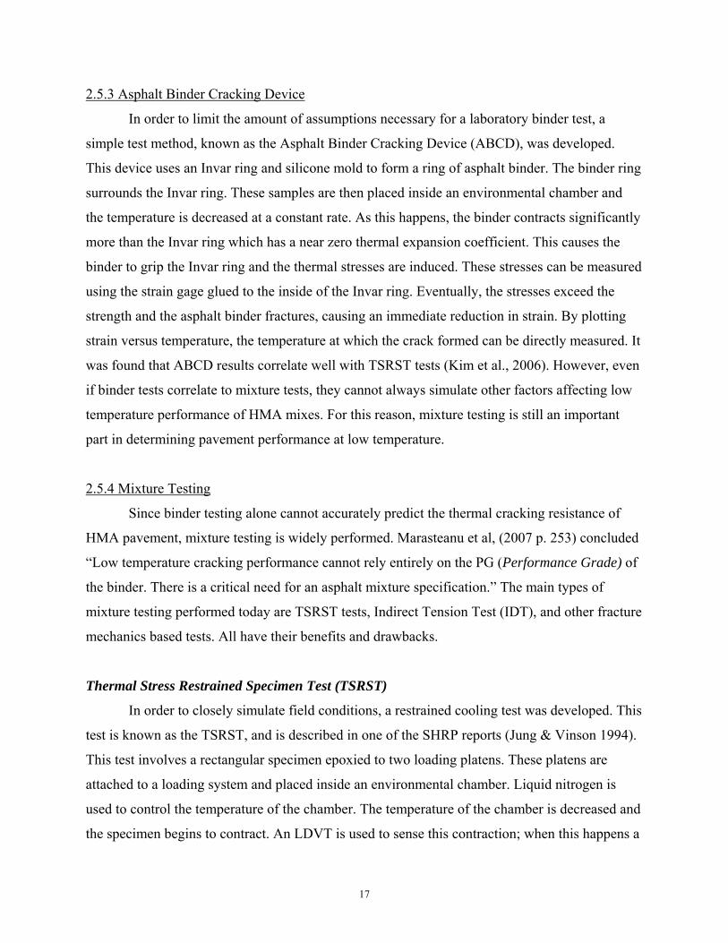
2.5.3 Asphalt Binder Cracking Device

In order to limit the amount of assumptions necessary for a laboratory binder test, a

simple test method, known as the Asphalt Binder Cracking Device (ABCD), was developed.

This device uses an Invar ring and silicone mold to form a ring of asphalt binder. The binder ring

surrounds the Invar ring. These samples are then placed inside an environmental chamber and

the temperature is decreased at a constant rate. As this happens, the binder contracts significantly

more than the Invar ring which has a near zero thermal expansion coefficient. This causes the

binder to grip the Invar ring and the thermal stresses are induced. These stresses can be measured

using the strain gage glued to the inside of the Invar ring. Eventually, the stresses exceed the

strength and the asphalt binder fractures, causing an immediate reduction in strain. By plotting

strain versus temperature, the temperature at which the crack formed can be directly measured. It

was found that ABCD results correlate well with TSRST tests (Kim et al., 2006). However, even

if binder tests correlate to mixture tests, they cannot always simulate other factors affecting low

temperature performance of HMA mixes. For this reason, mixture testing is still an important

part in determining pavement performance at low temperature.

2.5.4 Mixture Testing

Since binder testing alone cannot accurately predict the thermal cracking resistance of

HMA pavement, mixture testing is widely performed. Marasteanu et al, (2007 p. 253) concluded

“Low temperature cracking performance cannot rely entirely on the PG (Performance Grade) of

the binder. There is a critical need for an asphalt mixture specification.” The main types of

mixture testing performed today are TSRST tests, Indirect Tension Test (IDT), and other fracture

mechanics based tests. All have their benefits and drawbacks.

Thermal Stress Restrained Specimen Test (TSRST)

In order to closely simulate field conditions, a restrained cooling test was developed. This

test is known as the TSRST, and is described in one of the SHRP reports (Jung & Vinson 1994).

This test involves a rectangular specimen epoxied to two loading platens. These platens are

attached to a loading system and placed inside an environmental chamber. Liquid nitrogen is

used to control the temperature of the chamber. The temperature of the chamber is decreased and

the specimen begins to contract. An LDVT is used to sense this contraction; when this happens a

18

relay is sent to the loading system which applies enough tensile load to stretch the sample back

to its original length. This process continues until the sample breaks. During this test, the load

and temperature of the sample are constantly recorded. Thus, the failure stress and temperature

are easily determined from plots of stress versus temperature. Since this method fairly accurately

simulates field failure mechanisms, it is thought to be the best method available to evaluate an

HMA pavement’s low temperature cracking resistance. However, this test has several problems

that make it undesirable for a routine mixture test. Sample preparation can take considerable

amounts of time. This process includes slab compaction, sawing and drying of specimens, as

well as the alignment and epoxying of these specimens to the loading platens. The epoxy used to

affix the samples to the loading platens can take up to 24 hours to cure; this cure time limits the

number of samples that can be tested within a given time. Additionally, Jung and Vinson (1994)

also pointed out that sample alignment is critical since small eccentricities induce bending

stresses, which introduce variability into the results. Another disadvantage is the size of the

apparatus and the need for external loading equipment to perform the test. Also, even if one can

align and epoxy several samples at once, one would still need multiple apparatuses and a larger

chamber to accommodate them at one time. Often, this is impractical and thus severely limits the

number of samples that can be tested in a given time. Another problem noted is the high cost of

the chamber coolant (liquid nitrogen) (Epps, 1998). Due to all of these drawbacks, the TSRST is

not a routine test and other methods are used for regular mixture testing.

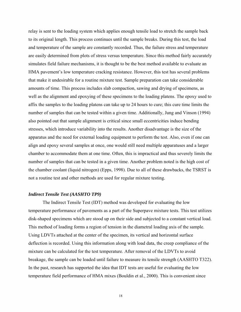
Indirect Tensile Test (AASHTO TP9)

The Indirect Tensile Test (IDT) method was developed for evaluating the low

temperature performance of pavements as a part of the Superpave mixture tests. This test utilizes

disk-shaped specimens which are stood up on their side and subjected to a constant vertical load.

This method of loading forms a region of tension in the diametral loading axis of the sample.

Using LDVTs attached at the center of the specimen, its vertical and horizontal surface

deflection is recorded. Using this information along with load data, the creep compliance of the

mixture can be calculated for the test temperature. After removal of the LDVTs to avoid

breakage, the sample can be loaded until failure to measure its tensile strength (AASHTO T322).

In the past, research has supported the idea that IDT tests are useful for evaluating the low

temperature field performance of HMA mixes (Bouldin et al., 2000). This is convenient since

19

IDT tests are simple to conduct and field samples can be readily obtained and tested. Multiple

samples can be cut from a single laboratory specimen or field core and several tests can be

performed per day.

However, this test method is often inaccurate when compared to TSRST results. A study

conducted by Epps (1998) found that, for several mixes, the TSRST cracking temperatures were

warmer than the IDT’s predicted cracking temperatures. Epps concluded the reason for this is the

number of assumptions that must be made to estimate the low temperature performance from the

data acquired using the IDT. These include assumptions on the field failure mechanism and the

thermal expansion coefficient of the mix. Another study performed by Marasteanu et al. (2007)

corroborated these findings. This study found that IDT test results using field samples showed

lower fracture strengths than TSRST. Being critical of the IDT, Marasteanu stated “The current

indirect tensile test provides useful information for the complete evaluation of low temperature

behavior of asphalt mixtures, but is not the best choice for a simple screening test.”

Fracture Mechanics Tests.

Fracture tests are another type of method for measuring the low temperature cracking

resistance of HMA pavements. Facture mechanics tests measure the energy required to break

mechanically loaded HMA samples and relate this information to low temperature cracking

performance. The important parameters obtained from these tests are fracture energy and fracture

toughness.

A study performed by Marasteanu et al. (2004) investigated several different fracture

mechanics based test methods. The three major fracture test geometries used in this study were

the Disk-Shaped Compact Tension Test (DSCT), Semicircular Bending Test and a bending beam

test. The DSCT test consists of a notched disk which is loaded in tension. The bending beam test

and the Semicircular Bending Tests both use simply supported specimens and subject them to a

vertical load at their midspan. The difference between them is the bending beam test uses a

rectangular beam specimen and the semicircular bending test uses a half disk specimen. All of

the three tests include a notch near the center of the sample. This notch produces a well defined

and predetermined area for crack initiation and growth. Measuring the load, deflection and crack

opening allows for the determination of stress and stain which provide fracture energy and

fracture toughness. However, these tests are limited by their assumptions. One of the most

20

important assumptions made for these tests is the selection of test temperature and loading rate.

Using the DSCT, Wagoner et al. (2005) found that fracture energy increased with increasing

temperature or decreasing loading rate. Marasteanu et al. (2004) found that the ranking of

different HMA mixes changed depending on the temperature. Li et al. (2006) demonstrated that

the change in fracture properties “levels off” at temperatures near the glass transition temperature

(p. 30). These studies demonstrated that simply making an assumption of a test temperature and

loading rate may not provide reasonable estimates of pavement performance and may even cause

incorrect ranking of mixture performance. This uncertainty is the major disadvantage with

predicting pavement performance from these tests; if care is not taken when selecting these

values, the results obtained will lead to false conclusions. In order to eliminate these problems,

an ideal test method should closely approximate field conditions, directly measure the failure

temperature of the sample and would be simple to use. One way to do this is the use of a fixed

frame restrained cooling test.

2.6 Fixed Frame Restrained Cooling Tests

Work by Monismith et al. (1965) first introduced the use of a fixed frame to measure

thermal response of a rectangular HMA sample. Almost a decade later, further work by Fabb

(1974) used a more elaborate test setup to perform restrained cooling tests. Both studies used

rectangular beam specimens which were epoxied to Invar loading frames. Both studies reduced

the temperature and measured the stress induced in the sample. While Monismith et al. did not

test the samples to failure, Fabb did. Thus, Fabb’s test results are more applicable for the test

method developed in this study (ACCD). One important finding by Fabb was that often the load

in the samples would not continue to increase up until fracture. Rather, they often showed a peak

value and would level off or even decrease before fracture. It was not known exactly why this

occurred. He found that the peak value temperatures were more repeatable than the temperate of

complete failure. It was also found that the peak temperatures were generally more repeatable

than the failure stresses. These findings would prove useful for the development and evaluation

of the ACCD test method.

21

In the development of his test device, Fabb showed considerable concern for errors due to

compliance and thermal shrinkage of the apparatus. Since contraction of the frame of the

apparatus due to thermal changes would relieve stress, and contraction of the “linkages” to which

the sample was epoxied would increase thermal stresses, he designed his device so these would

cancel each other. As for limiting the mechanical deformation of the apparatus, only control of

the crossectional dimensions of the parts could be used. Over 30 years later these concerns are

still key considerations of the proposed ACCD test. The next section will discuss the

development of the ACCD and evaluate its potential to predict low temperature performance of

HMA mixtures.

22

3. COEFFICIENT OF THERMAL EXPANSION (CTE) OF OHIO AGGREGATES

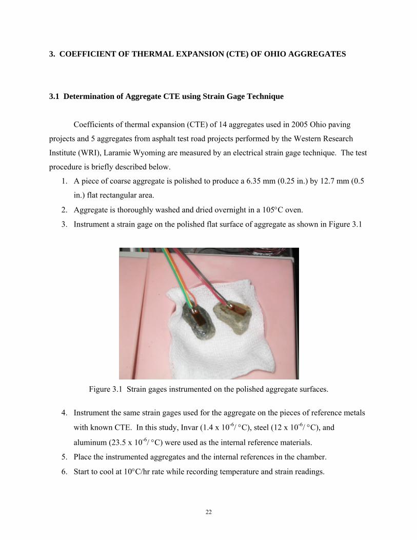
3.1 Determination of Aggregate CTE using Strain Gage Technique

Coefficients of thermal expansion (CTE) of 14 aggregates used in 2005 Ohio paving

projects and 5 aggregates from asphalt test road projects performed by the Western Research

Institute (WRI), Laramie Wyoming are measured by an electrical strain gage technique. The test

procedure is briefly described below.

1. A piece of coarse aggregate is polished to produce a 6.35 mm (0.25 in.) by 12.7 mm (0.5

in.) flat rectangular area.

2. Aggregate is thoroughly washed and dried overnight in a 105°C oven.

3. Instrument a strain gage on the polished flat surface of aggregate as shown in Figure 3.1

Figure 3.1 Strain gages instrumented on the polished aggregate surfaces.

4. Instrument the same strain gages used for the aggregate on the pieces of reference metals

with known CTE. In this study, Invar (1.4 x 10-6/ °C), steel (12 x 10-6/ °C), and

aluminum (23.5 x 10-6/ °C) were used as the internal reference materials.

5. Place the instrumented aggregates and the internal references in the chamber.

6. Start to cool at 10°C/hr rate while recording temperature and strain readings.

23

7. For each strain value, subtract the strain reading of Invar from all other strain readings at

the corresponding temperature. This step is for temperature compensation of strain gages.

8. Plot temperature versus the corrected strain as shown in Figure 3.2. Determine the slope

of the linear fits. Note that the slope of Invar is zero.

9. CTE is determined as the slope in Figure 3.2 plus 1.4 (CTE of Invar).

10. Check CTEs of steel and aluminum are close to 12 ± 1 and 23.5 ± 2 x 10-6/°C,

respectively. In the example in Figure 3.2, CTEs of steel and aluminum are 11.8 and

23.3 x 10-6/°C, respectively.

11. Report CTEs of aggregates. From Figure 3.2, CTEs of aggregates from Kansas, Arizona,

and Nebraska are 4.3, 7.2, and 10.6 x 10-6/°C, respectively.

The CTE measurement results of 19 aggregate are summarized in Table 3.1. The strain gage

technique measuring CTE of aggregate seems to work well and is repeatable. On average, the

difference between duplicate measurements (using the same instrumented aggregate pieces) is

0.3 – 0.4 x 10-6/°C. CTEs for Ohio aggregates range from the minimum of 4.0 x 10-6/°C for the

District 6 project to the maximum of 11.4 x 10-6/°C for one of District 3 projects.

Figure 3.2 Temperature versus the corrected strain to determine aggregate CTE.

y = 2.9x - 57.6

y = 5.8x - 119.7y = 9.2x - 178.2

y = 10.4x - 380.3

y = 21.9x - 545.8

-1200

-1000

-800

-600

-400

-200

0

-40 -30 -20 -10 0 10 20 30

Temperature, C

Mic

rost

rain

Aluminum

Steel

NEAZKS

Invar

24

Table 3.1 Coefficient of Thermal Expansion of 14 Aggregates from 9 Ohio DOT Districts and 6 Aggregates from WRI Test Roads

District/Agg ID

Coefficient of Thermal Expansion, με/°C

Run #1 Run #2 Average Difference

between 2 Runs Ohio Aggregates from 9 Districts

1B 7.2 7.8 7.5 0.61 1C 7.4 8.1 7.8 0.75

2D 6.2 7.0 6.6 0.88

3B 11.2 11.5 11.4 0.25 3C 5.5 6.0 5.8 0.46 3D 9.5 10.0 9.8 0.42 3E 6.1 5.8 6.0 0.29

4A 9.9 10.0 9.9 0.11

5B 4.6 4.7 4.6 0.07

6C 4.1 3.9 4.0 0.24

7D 4.7 4.9 4.8 0.24

8C 5.3 5.3 5.3 0.08

9A 7.7 8.1 7.9 0.39 9C 4.8 - 4.8

Ohio Aggregate Only Average 6.9 0.4 St Dev 2.3 0.3

Non-Ohio Aggregates Arizona 8.6 8.5 8.5 0.14 Kansas 5.9 5.5 5.7 0.39

Nebraska 7.5 7.4 7.4 0.06 Ontario (1) 6.6 6.9 6.8 0.27 Ontario (2) 5.4 5.6 5.5 0.25 Wyoming 9.1 9.1 9.1 0.00

All Aggregates Average 7.0 0.3 St Dev 2.0 0.2

25

3.2 Significance of Aggregate CTE in HMA Low Temperature Cracking

The CTE of asphalt mix is measured where the contraction of the mix during cooling is

allowed in all three spatial directions and both asphalt binder and aggregate are contracted.

However, in asphalt pavement under cooling, due to the longitudinal constraint and large

modulus difference between aggregate and asphalt binder, aggregate is contracted and asphalt is

extended. In other words, the asphalt binder in HMA under cooling is subjected to the thermal

strain (calculated by ΔT·αb) and additional mechanical strain due to contraction of rigid

aggregates. Since asphalt binder has much lower tensile strength than aggregate, accurate

determination of the magnitude of total stress in asphalt binder under cooling environment is

important.

In this section, composite models are used to understand the low temperature cracking of

asphalt pavement. First, CTE of HMA is calculated as a composite and is compared with values

determined by the current method, the rule of mixture. Second, the composite models are used

to attempt to explain the behaviors of asphalt binder, aggregates, and asphalt mixture during

cooling that leads to thermal cracking of asphalt pavement.

The recently introduced AASHTO mechanistic-empirical pavement design guide requires

CTE of asphalt mixes to evaluate the low temperature performance of a proposed asphalt

pavement. Since there is no standard test for determining CTE of HMA, the design guide

software computes it using mix volumetrics and CTEs of the asphalt binder and the aggregate

using the simple rule of mixture (ARA, 2004).

· ·

3 · 3.1

where,

αmix = linear thermal deformation coefficient of asphalt mix per °C VMA = volume percentage of voids in mineral aggregate (typically 15%) Bb = volumetric thermal deformation coefficient of asphalt binder per °C Vagg = volume percentage of aggregate in the mixture (typically 85%) Bagg = volumetric thermal deformation coefficient of aggregate per °C (12 – 34 x 10-6/°C

for Ohio aggregates) Vtot = total volume of mixture (100%)

26

Volumetric CTE is three times of the linear CTE. For typical binder, 510 x 10-6 ml/ml /°C (or

170 x 10-6 mm/mm /°C) is used as a default value at low temperature in AASHTO M 320 Table 1

specification (Bouldin et al., 2000). For Ohio asphalt mixes using local aggregates, the

calculated CTE using the Equation 3.1 ranges from 29 – 35 x 10-6 mm/mm /°C. These values are

somewhat different from values measured using dilatometric testing (Marasteanu et al., 2007)

and strain gage measurement (Stoffels et al., 1996). In the dilatometric measurement study, the

linear CTE of 36 laboratory and field mixes at low temperature ranged from 1.4-16 x 10-6

mm/mm /°C with 10.2 x 10-6 mm/mm /°C average measured under cooling condition temperature

below glass transition temperature. In the strain gage study performed at a temperature range

between 0 to 25ºC, the linear CTE of 22 field mixes at low temperature ranged from 13-30 x 10-6

mm/mm /°C.

The equation 3.1 for CTE of HMA oversimplifies the responses of asphalt binder and

aggregate to temperature changes. Mix CTE may be better approximated by considering the

asphalt mix as a composite of aggregates, asphalt binder, and air. Two particulate composite

models are used to describe HMA; Hirsch model and Counto model as shown in Figure 3.3. the

Hirsch model is a combination of a parallel model and a series model. The parallel model

assumes the same strain for both components under loading and the series model assumes the

same stress for both components (Young et al., 1998). A major drawback of the Hirsch model is

Figure 3.3 Composite models; Hirsch model and Counto model.

Parallel model

Series model

(a) Hirsch model (b) Counto model

27

that void (air) cannot be modeled since the void cannot carry load at the series portion of the

model (the composite collapses). The air in HMA is assumed to be uniformly distributed within

asphalt binder which can be represented by the Counto model shown in Figure 3.3 (b). The

inclusion of air would not affect CTE of asphalt binder. However, the modulus of the binder-air

mixture is affected by the inclusion of air voids and can be determined by Equation 3.2.

1 11 · ·

3.2

where,

EVMA = modulus of binder-air composite in VMA Eb = modulus of binder Ea = modulus of air ( = 0) Va = volume fraction of air (= percent air divided by VMA)

In general, the parallel model alone overestimates the moduli of composites and the series model

underestimates the moduli. The Hirsch and Counto models estimate values between the

estimations from the parallel model and the series model and are more realistic than both parallel

and series models. The mix CTE Equation 3.1 in the AASHTO mechanistic-empirical pavement

design guide is in the form of the parallel model, hence it tends to overestimate CTE of HMA.

To consider HMA as a composite, an idealized packing and a three dimensional phase

diagram of aggregates and asphalt binder are assumed as shown in Figure 3.4. In comparison to

asphalt binder CTE (150-200 x 10-6 per °C at low temperature), the aggregate CTE is relatively

small. However, the large volume fraction of aggregates in HMA and the orthotropic responses

of HMA to thermal contraction make the aggregate CTE a very important factor affecting low

temperature performance of HMA. As temperature drops, asphalt pavement behaves differently

in three mutually perpendicular directions (orthotropic). In the vertical direction, there is no

restraining and all thermal strain is realized as contraction leaving no thermal stress (pavement

gets thinner and free of stress in the vertical direction). In the longitudinal direction (direction of

traffic), pavement is restrained from contraction and thermal strain causes developing thermal

stress (pavement maintains the same length and is in state of stress). In the transverse direction

28

(perpendicular to the direction of traffic), it is speculated that pavement is restrained from

contraction by friction between the pavement and the underlying layer. Some of thermal stress

may be relieved by slip (pavement contracts some and is in state of lower stress than in

longitudinal direction). For this reason, considering one dimensional (in direction of traffic)

composition of asphalt mixture is important in determining the cracking temperature of asphalt

pavement. If 85% aggregate volume and 15% air plus asphalt binder volume (volume ratio of

5.7:1) within the asphalt pavement are assumed, an one-dimensional ratio in the longitudinal

direction between aggregate and binder can be calculated for simplified ideal packing with unit

cubic volume as shown in Figure 3.4. The volume fraction of aggregate in the phase diagram is

Lagg3 = 0.85 and, thus, Lagg = 0.9473 ( 3 aggregateoffractionvolume ) and Lb = 1 - Lagg = 0.0527.

The one-dimensional ratio of aggregate to binder is defined as length ratio (LR) and is about 18

for a typical asphalt mixture with 15% void in mineral aggregate (VMA) (Kim, 2005). The

asphalt binder in the parallel model represents the asphalt films sandwiched between two

aggregate surfaces aligned with the traffic direction. The asphalt binder in the series model

represents the asphalt films placed perpendicular to the traffic direction.

Figure 3.4. Idealized packing of aggregate and asphalt binder and 3-D cubic phase diagram.

Lb Lagg

Aggregate

Asphalt Binder

z

x

y

Parallel model

Series model

Traffic Direction

Aggregate

Asphalt

29

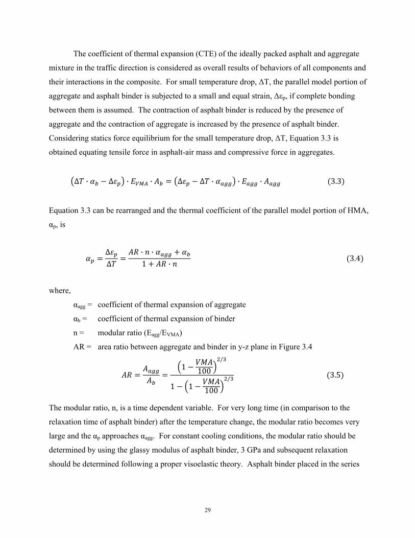
The coefficient of thermal expansion (CTE) of the ideally packed asphalt and aggregate

mixture in the traffic direction is considered as overall results of behaviors of all components and

their interactions in the composite. For small temperature drop, ΔT, the parallel model portion of

aggregate and asphalt binder is subjected to a small and equal strain, Δεp, if complete bonding

between them is assumed. The contraction of asphalt binder is reduced by the presence of

aggregate and the contraction of aggregate is increased by the presence of asphalt binder.

Considering statics force equilibrium for the small temperature drop, ΔT, Equation 3.3 is

obtained equating tensile force in asphalt-air mass and compressive force in aggregates.

∆ · ∆ · · ∆ ∆ · · · 3.3

Equation 3.3 can be rearranged and the thermal coefficient of the parallel model portion of HMA,

αp, is

∆∆

· ·1 · 3.4

where,

αagg = coefficient of thermal expansion of aggregate

αb = coefficient of thermal expansion of binder

n = modular ratio (Eagg/EVMA)

AR = area ratio between aggregate and binder in y-z plane in Figure 3.4

1 100

/

1 1 100/ 3.5

The modular ratio, n, is a time dependent variable. For very long time (in comparison to the

relaxation time of asphalt binder) after the temperature change, the modular ratio becomes very

large and the αp approaches αagg. For constant cooling conditions, the modular ratio should be

determined by using the glassy modulus of asphalt binder, 3 GPa and subsequent relaxation

should be determined following a proper visoelastic theory. Asphalt binder placed in the series

30

Figure 3.5 Poisson’s effect of asphalt binder coated on aggregate surface.

portion of composite model is also subjected to the Poisson’s effects as shown in Figure 3.5.

Since contraction of binder is prohibited in y and z directions, binder is in tension with

magnitude of ΔT ( b – p) in y and z directions for ΔT temperature drop.

The total strain of the mix, Δεmix, for the small temperature drop, ΔT, is

∆ ∆ · ∆ · 2 3.6

Poisson effect of aggregate is ignored since the difference between αagg and αp is very small.

CTE of total mix, αmix, is estimated by equation 3.7 as a function of mix volumetrics (VMA and

percent of air) and physical properties of components (moduli, CTE, and Poisson’s ratio).

∆

∆ 2 3.7

where,

Lagg = linear fraction of aggregate in Figure 3.4

1 100

/

3.8

Lb = 1 – Lagg = linear fraction of binder in Figure 3.4

ν = Poisson’s ratio of binder

Binder at To

Binder at To – ΔT without adhesion

Binder adhered to aggregate surface at To – ΔT

Aggregate surface

Contraction due to binder CTE

Contraction due to Poisson’s effect

31

The ranges of CTE values for asphalt mixes determined by the composite model (Eq. 3.7) and

the rule of mixture (Eq. 3.1) are presented in Table 3.2. CTEs of mixes estimated by the

composite model are about 8-10 x10-6/ºC lower than the values estimated by the rule of mixture

method and are agree well with the values reported by Stoffels et al., (1996), 13-30 x 10-6 /°C for

various asphalt mixes tested. Estimation of thermal contraction of asphalt mix using a composite

model that utilizes Hirsch’s model and Counto’s model seems reasonable.

The sensitivities of the composite model CTE for various factors are summarized in

Table 3.3. In the composite model, the binder CTE is the most important factor affecting the mix

CTE followed by VMA and the aggregate CTE. Poisson’s ratio of binder also has minor effects

on the mix CTE. The effects of percent air and the binder modulus on the mix CTE are less than

1.0 x 10-6/ºC and are negligible. When the rule of mixture is used, the effects of VMA and

binder CTE on the mix CTE are larger than the estimations by the composite model.

Table 3.2 CTE of Asphalt Mixes Predicted Using the Composite Model and the Rule of Mix.

VMA % 

CTE of mix determined by  Composite model, 10‐6 /°C (Eq 3.7) 

CTE of mix determined by  Rule of Mix, 10‐6 /°C (Eq 3.1) 

Aggregate CTE, 10‐6 /°C  Aggregate CTE, 10‐6 /°C 5  7  9  11  5  7  9  11 

12  17.0  18.9  20.7  22.6  24.8  26.6  28.3  30.1 13  18.1  19.9  21.8  23.6  26.5  28.2  29.9  31.7 14  19.2  21.0  22.8  24.7  28.1  29.8  31.5  33.3 15  20.3  22.1  23.9  25.7  29.8  31.5  33.2  34.9 16  21.4  23.2  25.0  26.8  31.4  33.1  34.8  36.4 

17  22.5  24.3  26.0  27.8  33.1  34.7  36.4  38.0 Assume Air % = 4,       Eagg = 70 GPa,           Eb = 3 GPa,      νb = 0.35,       αb = 170x10

‐6 /°C 

32

Table 3.3 Sensitivity Analysis of Mix CTE Determined by Composite Model

Unlike the conditions used in mix CTE determination where contraction of mix in all

directions are allowed, the contraction of asphalt pavement in the longitudinal direction is not

permitted in cooling of field pavement. The compatibility condition of cooling pavement

requires that, for temperature drop ΔT, the magnitude of thermal contraction equals to the

magnitude of extension by tensile stress (or thermal stress) as given in Equation 3.9.

∆ · ∆ · 2 3.9

where,

Ep = modulus of parallel model portion of mix = Eagg Aagg + EVMA Ab

σ = thermal stress

σ/EVMA = Δεb = true binder strain in the mix

σ/Ep = Δεagg = true aggregate strain in the mix

From above two relationships, Δεagg = Δεb (EVMA/Ep)

Since the strength of asphalt binders (less than 8 MPa) is much smaller than the strength of

aggregates (larger than100 MPa), the strain of asphalt binder is of interest. The contraction (the

  

Parameter Range  Difference by Composite model  (Eq 3.6), 10‐6 /°C 

Difference by Composite model  (Eq. 3.1), 10‐6 /°C Min  Max 

Air, %  0  10  ‐0.6  NA VMA, %  12  17  5.3  8.2 Poisson’s ratio of binder, ν 

0.35  0.5  2.5  NA 

Eb, GPa  0.0001  3  0.4  NA ν, Eb   0.35, 3GPa  0.5, 100kPa  2.0  NA Eagg, GPa  20  200  ‐1.4  NA 

αb, 10‐6 /°C  200  400  17.9  29.1 

αagg, 10‐6 /°C  5  11  5.5  5.2 

parallel model

contraction

series model

contraction

series model

extension

parallel model

extension

33

left side of equation) is governed by CTE of components and the extension (the right side of

equation) is governed by the moduli of components. The effective binder CTE (α’b) for the mix

can be obtained by rearranging Equation 3.9.

∆∆

2

1 3.10

where,

αp = the thermal coefficient of parallel model portion of HMA, given in equation 3.4

∆∆

· ·1 · 3.4

αagg = coefficient of thermal expansion of aggregate

αb = coefficient of thermal expansion of binder

n = modular ratio (Eagg/EVMA)

AR = area ratio between aggregate and binder in y-z plane in Figure 3.4

1 100

/

1 1 100/ 3.5

LR = length ratio

1 100

/

1 1 100/ 3.11

n’ = modular ratio (Ep/EVMA)

ν = Poisson’s ratio of asphalt binder, 0.35

Table 3.4 summarizes the effective CTE of asphalt binders for various combinations of

VMA and aggregate CTE. In all cases, the effective asphalt binder CTE is much larger than the

asphalt binder CTE by 50 – 100%. For given asphalt binder, the decease of VMA of HMA from

17% to 12% increases the effective CTE by 9 - 35 x 10-6/ºC. The change of aggregate CTE form

5 to 11 x 10-6/ºC increases the effective CTE by 60-80 x 10-6/ºC. According to this composite

model analysis, the most susceptible asphalt mix is one with low VMA and with aggregate with

high CTE.

34

To illustrate the difference between the simple rule of mixture and the composite model

in predicting tensile stress in asphalt mixes, let us consider two asphalt mixes with the same

asphalt binder with 170 x 10-6/°C CTE, but one mix with 12% VMA and aggregate with 11 x 10-

6/°C CTE and the other with 15% VMA and aggregate with 5 x 10-6/°C CTE. In the AASHTO

Mechanistic-Empirical Pavement Design Guide, the CTE (αmix) of the two mixes can be found

from Table 3.2 and are 30.1 and 29.8 x 10-6/°C, respectively. In the mechanistic analysis, for an

instantaneous temperature drop ΔT, the mixes are considered at the stress level determined by

ΔT·αmix·Emix(T). The relaxation modulus of mix at temperature T, Emix(T), for instantaneous

time interval and at near cracking temperature, would approach the glassy modulus which are

usually considered constant for various asphalt mixes. In other words, these two mixes are

considered to develop the same magnitude of thermal stress under the same cooling environment.

The rate of stress relaxation will be determined by the master relaxation modulus curve and

temperature-shift factor relationship for each mix.

According to the composite model, the mix with 12% VMA and aggregate with 11 x 10-

6/°C CTE will cause asphalt binder to be in a 37% higher stress level than the mix with 15%

VMA and aggregate with 5 x 10-6/°C CTE (339 versus 248 x 10-6/°C from Table 3.4). The stress

level in asphalt binder can be determined from ΔT·α’b·Eb(T). In these two asphalt mixes, asphalt

binder will be subjected to different magnitudes of thermal stress and will be subjected to the

same rate of stress relaxation.

Table 3.4 Effective Asphalt Binder CTE in HMA.

VMA % 

Effective Asphalt Binder CTE, 10‐6 /°C at Cold Temperature near Cracking 

Aggregate CTE, 10‐6 /°C 5  7  9  11 

12  255  283  311  339 13  252  278  303  329 14  249  273  297  321 15  248  270  292  314 16  247  267  288  309 

17  246  265  285  304 Assume Air % = 4,   Eagg = 70 GPa,     Eb = 3 GPa      νb = 0.35      αb = 170x10

‐6 /°C 

35

In summary, the current mechanistic procedures, including the AASHTO Mechanistic-

Empirical Pavement Design Guide, do not recognize the composite nature of an asphalt mixture

in the low temperature cracking phenomenon. The Equation 3.1 used in the mechanistic

procedures generally overestimates the mixture CTE and does not include the effects of

aggregate CTE in thermal cracking of asphalt pavement. The indirect tensile (IDT) creep and

strength tests, commonly used for laboratory characterization of asphalt mixes for low

temperature performance, are performed at a constant temperature and cannot evaluate the

aggregate CTE effects either. However, the use of the composite model and Equation 3.10 to

estimate stress development in asphalt phase in the HMA is not possible at the present time. Due

to lack of test devices and procedures, the CTEs of asphalt binder and aggregate cannot be

routinely determined. Until an improved test device and procedure become available, a

laboratory test method that simulates the field pavement conditions, such as Thermal Stress

Restrained Specimen Test (TSRST), is recommended to characterize the low temperature

cracking potential.

36

4. FIXED FRAME WITH AN EPOXIED CYLINDRICAL SAMPLE

As discussed in the literature review, the current test methods for evaluating the low

temperature performance of HMA do not meet the criteria set forth for the ideal test method.

None of the current test methods, with the exception of the TSRST, directly measure the failure

temperature by closely simulating field conditions. Many use approximations and assumptions to

convert measured data into an estimate of low temperature cracking potential. Some of these

tests require assumptions on material properties, while others require testing at certain

temperatures and inferring properties based on these results (like the BBR/DTT in PG grading).

In this regard, the TSRST has the advantage since failure occurs as the specimen is restrained

and is slowly cooled. If not for the complicated equipment necessary to perform the test, the

limited number of samples that can be tested at once and the extensive sample preparation, this

test may be an excellent routine test to evaluate the low temperature cracking resistance of HMA

mixes. Thus, the purpose of this study was to design and validate a simple apparatus to directly

measure the low temperature cracking resistance of HMA mixes by simulating field failure

mechanisms through gradual cooling of a restrained specimen. However, rather than using a

mechanical loading system as in TSRST, Invar steel, which has a low thermal expansion

coefficient (approximately 0.5-2 x10-6 per °C), was used to induce the tensile stresses in HMA.

However, during the development process, it was found that this fixed frame method had

very poor repeatability. Variations in cracking temperature up to 10°C were observed for a given

mix. This variability was due to the fact that this test method suffers from specimen alignment

problems, stress concentrations near the glued ends of the specimen, and compliance problem of

the loading-frame. For these reasons it was decided to abandon the fixed frame ACCD in favor

of a new method, the concentric ring ACCD to be discussed in section 5. Although the fixed

frame apparatus did not produce acceptable results, with further development this test method

may be viable. For this reason, the fixed frame device is briefly presented in order to facilitate

further research with this or similar fixed frame restrained cooling devices. For a more detailed

description of the final test procedure or the developmental history of the procedure, refer to

Appendix A.

37

4.1 Summary of the Test Procedure

During the Superpave mix design process, many 150mm gyratory samples are produced

for the volumetric analysis. After determining the optimum asphalt content these samples are

discarded. In order to utilize these samples to evaluate the low temperature performance of an

asphalt mix, a fixed frame restrained cooling test was developed. For this test, cylindrical

samples with outer diameters of 70.6 mm are cored from the original 150 mm gyratory samples

by the use of a coring bit. Then, in order to produce a smooth surface, both ends of the cylinder

are sawn flat. This yields a sample that is approximately 100 mm tall and 70.6 mm in diameter.

The height to diameter ratio of the cored specimen (100/70.6) is much smaller than a typically

required (2/1) ratio. For ductile or granular materials, the ratio between height and diameter is

critical in tensile or compressive failure test since the failure mode of these materials is shear

phenomenon. The maximum shear plane in uniaxial test is 45° from horizontal. If the specimen

height is short, the end restrainment affects the test result significantly. It is important to keep a

2/1 height to diameter ratio for ductile or granular materials. However, in tensile failure of brittle

materials (HMA in very low temperature), the failure happens through the maximum tensile

plane which is horizontal and is less likely affected by the end restrainments.

As shown in Figures 4.1 and 4.2, the test device developed to test HMA consists of a

rigid steel base plate with a raised circular loading platen in the center. Three holes to hold Invar

rods are spaced evenly around the base-plate (120° apart each other). Before testing, an

alignment frame is placed in these holes. This frame is used to center the sample in the apparatus.

Once the alignment screws are centered, the sample is removed from the frame and both ends of

the sample are coated with epoxy. Since the alignment screws have not been moved from their

centered position, the sample is then returned to the center of apparatus. Next, the top loading

platen is placed onto the sample. Attached to this loading platen is a large diameter threaded

screw. A plate with a hole in the center is then positioned on top of the alignment stand. This

plate centers the top loading platen on the sample. The excess epoxy is then smoothed into a

fillet. After the epoxy cures for 24 hours, the alignment frame is removed and the test frame is

assembled.

Immediately before testing, a large tightening nut is tightened to restrain the sample from

contracting without inducing measurable tension in the frame. The test frame is then placed in an

38

environmental chamber and preconditioned for 15 minutes at 0°C. After this preconditioning, the

sample is then cooled at constant rate of 10°C/hr. As the setup cools, the HMA sample and the

steel attempt to contract; however, since the Invar prevents this, tension builds up in the HMA

sample. This tensile load is measured by strain gages attached to the Invar frame. As the

temperature continues to decrease the tensile stresses in the sample (and thus compressive stress

in the frame) increase up until the point where the induced stresses exceed the tensile strength of

the HMA mix. This causes a crack to form and a sudden reduction of stresses (and thus strain) is

observed. The temperature at which this jump in strain occurs is identified as the cracking

temperature (refer to Figure 4.3).

Figure 4.1 The fixed frame test setup during alignment.

12.7 mm (0.5 in.) dia. Invar

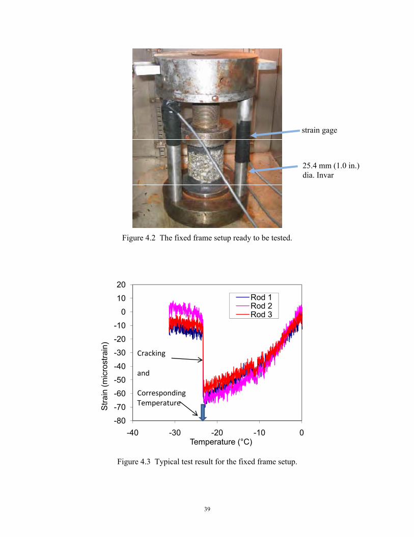
39

Figure 4.2 The fixed frame setup ready to be tested.

Figure 4.3 Typical test result for the fixed frame setup.

-80

-70

-60

-50

-40

-30

-20

-10

0

10

20

-40 -30 -20 -10 0

Stra

in (m

icro

stra

in)

Temperature (°C)

Rod 1Rod 2Rod 3

Cracking

and

CorrespondingTemperature

strain gage

25.4 mm (1.0 in.) dia. Invar

40

4.2 Fixed Frame Test Results

Initially, the fixed frame test device used 3 invar rods with 0.5 in. diameter as shown in

Figure 4.1. When tested with various asphalt mixes, fracture could not be induced by lowering

temperature due to excessive compressive deformation of the 3 invar rods (compliance problem).

The diameter of the 3 invar rods increased to 1.0 in. as shown in Figure 4.2 and was able to

induce fracture within the test specimens.

To determine the repeatability, 13 samples of known gradation were prepared for testing

using the fixed frame ACCD. These samples were cored from 6 inch diameter gyratory samples.

One group of test specimens consisted of six samples: two of coarse gradation, two of medium

gradation and two of fine gradation all with asphalt contents of 6.0%. The gradations of these

mixes are shown in Figure 4.4. The other group of samples was of the course gradation and had

asphalt contents 5.4%, 5.9% and 6.4%.

Initially, chamber air temperature was used to record cracking temperature to quickly

determine the repeatability of the test. Later, a dummy specimen containing a temperature

sensor at the middle is used to record the cracking temperature. The temperature at the center of

the dummy specimen is about 7.2°C warmer than the chamber air temperature.

Figure 4.4 Aggregate gradations used in the mixes for the fixed frame test.

1912.5

9.5

4.75

2.36

1.18

0.6000.3000.1500.075

0102030405060708090

100

Perc

ent P

assi

ng

Sieve Size, mm

0.45 Power Chart (12.5mm NMS)

ODOT SpecCoarseMediumFine

41

As is shown in Table 4.1, the repeatability of this fixed frame test was poor. The range in

cracking temperature was wide within a given sample group. Some mixes show differences in

cracking temperature of approximately 10°C between samples. Many factors may have

contributed to this high variability and these will be discussed in the following section.

Table 4.1 Summary of Fixed Frame Test Results.

Cracking Temperature (°C) Temperature Difference

Sample ID (Air Temp) (Dummy Temp) (Dummy-Air)

6.4% (a) 6.4% (b) 6.4% (b)

-32.30 -35.70 -25.40

Na Na Na

na na na

5.9% (a) 5.9% (b)

-37.50 -36.40

Na Na

na na

5.4% (a) 5.4% (b)

-43.60 -35.70

Na Na

na na

Coarse (a) Coarse (b)

-40.80 -37.90

-33.70 -30.80

7.10 7.10

Medium (a) Medium (b)

-35.80 -35.80

-28.65 -28.10

7.15 7.70

Fine (a) Fine (b)

-41.30 -31.60

-34.10 -24.40

7.20 7.20

42

4.3 Areas of Concern with the Test Method

There were problems and difficulties associated with the current apparatus and method of

testing. Some of these problems can be overcome by changing the test setup or procedure, while

others are difficult to avoid. The areas of difficulty may be linked to several aspects of the test

including: epoxying, alignment, sample geometry, apparatus problems and the time consuming

test procedure.

4.3.1 Sample Geometry

As previously indicated, sample preparation for this test method is extensive. First, HMA

specimens must be compacted using the gyratory compactor. Next, they must be cored with a

diamond tip coring bit. Finally, both ends of the sample must be sawn using a masonry saw. Not

only is this process time consuming and potentially hazardous, it has the potential to introduce

significant variability into the test specimens. It was found that the coring bit used to core the

samples had a tendency to wander slightly as it advanced through the gyratory compacted

specimens. This produced samples that were not perfectly straight. While some wandering of the

bit is unavoidable, by coring slowly, this problem was minimized for the 13 samples of known

gradation. In the future by using a more precise coring apparatus, distortions due to this effect

can be minimized. After coring, the samples were then sawn on both ends. Obtaining consistent

alignment of the samples perpendicular to the saw proved to be difficult. Due to the flexing of

the saw and misalignment of the specimens, some of the sample ends were not perfectly parallel.

Attempts to improve the parallelism of the samples after the initial cut resulted in the ends not

being flat or smooth. The use of a more rigid saw and an alignment device to aid in the

positioning of the samples would help to produce more repeatable sample geometries.

Another concern with the sample preparation process is the fact that the gyratory

compaction produces samples that are anisotropic in nature. Research has shown that gyratory

samples have higher air void concentrations near the sample ends (Chehab, O'Quinn, & Kim,

2000). There is also crushing of the aggregate near the ends of the sample. Since all samples

failed near the ends, these irregularities could potentially affect the test results. In order to

minimize the effects from prefractured aggregate and air void concentrations, taller gyratory

compacted specimens may be prepared and larger saw cuts taken from each end.

43

4.3.2 Epoxying

Several concerns arise from the fact that the sample needs to be epoxied in place on the

apparatus. These are difficult to avoid since the entire apparatus is designed around the sample

being epoxied to the loading platens. Regardless of any possible design changes, epoxy would

still be an intrinsic part of the test procedure. The most important problem involving epoxying is

curing time. Typically, a curing time of at least 24 hours was necessary. Thus, the time required

to test a single specimen with the fixed frame ACCD is restricted by this long curing time. This

limits the number of samples that can be tested in a given time. The way to remedy this would be

to have several loading platens and alignment frames.

An additional concern with the use of epoxy is that its application is difficult to conduct

cleanly, since the apparatus, the operator and the specimen itself may become soiled with excess

epoxy. Additionally, after the test is complete the epoxy must be removed from the loading

platens. This means heating the platens up to 150°C and scraping them clean. The platens must

be then allowed to cool before the rest of the cleaning procedure can be performed. Due to the

large thermal mass, this cooling takes several hours; this further increases the turn around time

for the test apparatus. Bonding is also a consideration with epoxying. If the platens are not

cleaned properly bond failure between the epoxy and the metal platens may result. This will

make any test results meaningless and the sample will be wasted.

Creating an adequate chamfer with the epoxy is also difficult. Keeping the chamfer

uniform around the circumference and the same on both ends of the sample is challenging.

Keeping this chamfer consistent from test to test is also difficult. It is not known what effect

these differences have on the fracture temperatures. However, since the samples fail near the end,

it is suspected that the type of chamfer may have a significant effect on the stresses induced at

the specimen ends. With practice and standardized equipment, uniform chamfers may be

produced.

4.3.3 Alignment

Horizontal alignment is another difficulty associated with this test method. For all of the

tests performed only rudimentary alignment was possible. This involved tightening three screws

placed at 120 degrees from each other an equal number of turns. These screws were positioned at

approximately mid height of the sample. Thus, they centered the middle of the sample

44

reasonably well. However, since some samples were not perfect cylinders, the sample ends were

not centered on the loading platens. It is impossible to determine the amount of eccentricity that

was induced using this method. This is extremely important because, as observed with TSRST

tests, even small eccentricities can have significant effects on the stress distribution in the sample

(Jung & Vinson, 1994.) It is believed that these irregular stress distributions are a major cause of

the variability observed in the measured cracking temperatures. Like horizontal alignment,

vertical alignment was also a significant concern associated with this apparatus. The fixed frame

ACCD currently has no method for assuring that the samples are standing perpendicular to the

loading platens. If the ends of the samples are not exactly parallel or flat, the sample will not be

perpendicular to the loading platens. Thus, the stress distributions in the samples are not pure

tension. It is believed that these variations were a significant source of the observed variability in

cracking temperatures.

4.3.4 Apparatus Problems

There were also physical problems with the apparatus itself, the most significant of which

was the sensitivity of the main screw. If small amounts of aggregate or binder were present in the

threads it would not function. Thus, careful cleaning and lubrication of the apparatus was a

necessity. The threads were also prone to physical damage. If the threads were damaged,

alignment was not possible until the bur on the thread had been removed.

All of these the problems with the screw would cause the apparatus to bind as the

tightening nut was being tightened during the epoxying/alignment procedure. This sudden

seizure of the tightening nut, which had considerable angular momentum, would cause the

spinning of the top loading platen and cause the alignment frame to move. In addition, this would

spread the epoxy and misalign the sample, making it necessary to perform the epoxying

/alignment procedure again. Such sensitivity is not desirable when attempting to develop an

apparatus that will be used in a routine test.

4.3.5 Test Problems

There were also problems with the test procedure itself. First and foremost was the

problem of end effects. All samples broke at one of the ends, thus end effects have significant

influence on the stresses present at the failure region of the sample. Due to the fact that the

45

sample must be glued into place, end effects are unavoidable. In order to eliminate the influence

of end effects on the failure of the sample, a notch may be introduced at the mid height of the

sample. This would create a predetermined failure zone. This would further increase the already

extensive sample preparation process and would introduce another potential variability in sample

geometry. Also, decreasing the cross section would limit the maximum aggregate size that could

be tested using this device.

Thermal strain in the apparatus itself is also a problem. The Invar rods do experience

some physical shortening due to thermal effects. Thus, since the sample is not completely

restrained, some of the strain in the HMA sample is relaxed. However, the steel screw connected

to the top loading platen also experiences considerable thermal strain. This increased thermal

load has a canceling effect on the previously mentioned relaxation. The magnitudes of these

strains can only be estimated. While the deformation of the Invar rods is the same for all samples,

the stress induced on the sample by the thermal contraction of the steel varies inversely with

sample height. Taller samples have less steel between their top end and the tightening nut. This

means samples exactly identical in all aspects except height, may have different cracking

temperatures due to the difference in thermal expansion of steel and the HMA mixture.

4.4 Benefits of the Test Method

Despite its difficulties, the fixed frame ACCD does have some advantages over other

procedures in use today for determining low temperature cracking resistance of HMA mixtures.

Unlike most other test methods, no complicated loading equipment is necessary. Only an

environmental chamber, a computer and a data acquisition system are required beyond the

apparatus itself. Additionally, unlike other test methods, the cracking temperature is easily and

directly determined. On all successful tests, the crack was sharp and clearly defined. With further

development, this test method may prove useful in determining the low temperature cracking

resistance of HMA mixtures.

46

5. CONCENTRIC RING ACCD APPARATUS

A significant amount time and resources had been spent to develop a test procedure for

the originally proposed fixed frame test for evaluating low temperature performance of asphalt

mix. However, the test results indicated that the test was not simple and did not produce

repeatable results as discussed in the previous section. A new asphalt concrete cracking device

(ACCD) in a ring shape was designed and a prototype was manufactured. To improve the signal

quality of the experiment, the quarter-bridge configuration of the strain gage was changed to

half-bridge configuration and the temperature sensors were changed from thermo-couple type to

resistance temperature detector (RTD). A new data acquisition system was built to

accommodate the improvement in the sensor. The new data acquisition system can test up to

four samples at the same time.

Like the fixed frame test, the new concentric ring test method also uses the low thermal

expansion coefficient of Invar steel to induce tensile stresses in an HMA specimen as the

temperature decreases. However, rather than relying on a rectangular or cylindrical specimen

epoxied to an Invar frame, the new method uses an Invar ring surrounded by an HMA sample

compacted in a ring shape as shown in Figure 5.1. The new test set-up eliminated the trimming

and gluing step with epoxy which shortened the specimen preparation time by 2 days and

significantly reduced the specimen alignment problem.

Figure 5.1 ACCD ring (at the center) with HMA compacted outside.

47

The key component of this test method is an Invar ring with a 101.6 mm (4 in.) outer

diameter, a 76.2 mm (3 in.) inner diameter, and 68.6 mm (2.7) in. height. This ring is

instrumented with a strain gage rosette and a temperature sensor on the inside wall of the ring. A

254 mm (10 in.) diameter sample of asphalt is then compacted around this ring at high

temperature. The sample is then placed inside an environmental chamber and the instrumentation

is connected to the data acquisition system. Then, the sample is preconditioned and cooled at a

constant rate. As the temperature inside the chamber is lowered the asphalt mix attempts to

contract. However, its contraction is prevented by the presence of the Invar ring. This causes

thermal stresses in the sample. At higher temperatures, these stresses can be relieved by viscous

flow of the asphalt binder in the mixture. However, as the temperature becomes lower, the

viscous flow gets slower and the thermal stresses begin to accumulate. These stresses cause the

HMA to grip the Invar ring tighter and tighter as the temperature drops. This inward pressure on

the Invar ring is evident by viewing the strain readings of the strain gage on the interior of the

ring. Ultimately, the stress that is developed in the HMA sample becomes greater than the tensile

strength of the HMA and the sample cracks. This crack is evident by a reduction in the strain

readings on the Invar ring. The temperature at which this stress is released is defined as the

ACCD cracking temperature. The development of this procedure is described in detail in the

following sections.

5.1 Design of the Apparatus

At the beginning of this project, the theory discussed above was only an idea and the

entire apparatus had to be completely designed. Due to the size and dimensions of the apparatus,

minimizing the weight of the device was important. Thus, aluminum was used for fabricating a

majority of the apparatus except the ACCD ring. The dimensions of the HMA ring were selected

considering the size of aggregates used in surface mixes. Adequate specimen dimensions are

necessary to ensure that the properties measured during the test are representative of the true

mixture properties. Selecting an adequate cross section for a given maximum aggregate size

ensures that the results are not significantly influenced by the distribution of large aggregate

particles within the specimen. Since the course aggregate particles of surface mixes are generally

48

small, the minimum cross-section area for cracking was selected to be 63.5 mm x 76.2 mm (2.5

in. x3 in.). Two variations of the apparatus to mold the sample were used during this project.

Variation 1 (one piece mold) is shown in Figure 5.2 and variation 2 (two piece mold) is shown in

Figure 5.3. Variation 2 was deemed to be superior since it was lighter and easier to clean than

Variation 1.

Figure 5.2 Concentric ring ACCD long mold (variation 1) after compaction.

Figure 5.3 ACCD concentric ring short mold (variation 2) after compaction.

49

5.1.1 Long Mold ACCD (Variation 1)

The most important part for the setup is a 68.6 mm (2.7 in.) tall Invar ring with an outer

diameter of 101.6 mm (4 in.) and an inner diameter of 76.2 mm (3 in.). A bi-axial strain gage and

a temperature sensor are fixed to the inside of this ring. The major axis of the strain gage is

aligned with the hoop direction of the ring, and the minor axis is 90° perpendicular to that. A

connection for attaching the instrumentation to the data acquisition system is also present inside

this ring. The top of the ring is notched to hold a collar to protect the instrumentation during the

sample compaction. This collar was machined from a stainless steel rod and has the same

diameter and approximately the same height as the ring. An aluminum foil cap is placed on top

of the collar to prevent HMA from falling into the instrumentation during compaction.

The base of this apparatus is a 304.8 mm x 304.8 mm (12 in. x 12 in.) square aluminum

plate 12.7 mm (0.5 in.) thick. A 2.5 mm (0.1 in.) deep ring of material was then removed from

this base-plate. This ring shape depression has an outer diameter of 273.8 mm (10.78 in.) and an

inner diameter of 76.2 mm (3 in.). This leaves a raised circle of aluminum in the center of the

plate that is perfectly concentric with the outer diameter of the cut in the base plate. This inner

circle is where the Invar ring will sit during specimen compaction.

A 171.5 mm (6.75 in.) tall 9.9 mm (0.388 in.) thick aluminum ring with an inner diameter

of 254 mm (10 in.) is used to form the outer diameter of the sample. This ring sits perfectly

inside the outer diameter of the recess made in the base-plate. Thus, when assembled on the

base-plate, the Invar ring and the aluminum ring are concentric and will form a 254 mm (10 in.)

outer diameter, 101.6 mm (4 in.) inner diameter ring of the HMA sample.

As shown in Figure 5.4, an aluminum pressing head in the shape of a ring is used to

compact the sample. The pressing head has an outer and inner diameter slightly smaller than 10

in. and greater than 101.6 mm (4 in.), respectively. This clearance allows the pressing head to

easily move vertically between the ACCD ring and the outer mold. Additionally, an extraction

frame was later developed to facilitate the extraction of samples after compaction.

50

Figure 5.4 ACCD mold and pressing head.

5.1.2 Short Mold ACCD (Variation 2)

While the Invar rings and the collar were the same, the second test setup had slight

changes in the other components. The base plate was now a circular plate with an outer diameter

of 254 mm (10 in.). A small circular 3.2 mm (0.125 in.) thick, 76.2 mm (3 in.) outer diameter

disk was bolted to the center of the base plate. This base plate has the advantage of being easier

to manufacture than the original base plate. Additionally the outer ring was only 86.4 mm (3.4 in.)

tall and 8.9 mm (0.35 in.) thick. An outer collar of the same thickness and 81.3 mm (3.2 in.) tall

was used to sit on top of this ring. This has two benefits over the taller outer ring used in the first

method:

1) Once compacted, the collars can be removed and the sample/ring/baseplate assembly

weighs less, making it easier to move the apparatus.

2) It is easier to clean.

For both variation 1 and variation 2, a 6.35 mm (0.25 in.) thick aluminum plate ring [outer

diameter 254 mm (10 in.) and inner diameter of 88.9 mm (3.5 in.)] was used to support the

samples during transporting and testing to minimize distortion of the sample. The development

of the testing procedure is described in section 5.2.

51

5.2 Development of the Test Method

Once the apparatus was designed, a sample preparation and testing procedure needed to

be developed. For this step, loose HMA from a paving project site was used to conduct eight

initial tests. Important developments during this stage of the procedure were: the compaction of

the sample, the extraction of the sample, the introduction of a notch aligned with the strain gage,

the lubrication of the Invar ring and determining how to distribute the HMA in the mold prior to

compaction. Each of these is described in further detail in this section.

It was found that varying compaction load produced different air voids. Using a 78.6 kN

(17,660lb), 267 kN (60,000lb), 445 kN (100,000lb) and 3 x 445 kN (100,000lb) (445 kN

repeated three times) static loads produced percent air voids of 13.3%, 7.6%, 6.6% and 5.1%,

respectively. For the latter three maximum 445 kN (100,000lb) static loads were applied to the

sample, each were held for 15 seconds. This means that once the load on the sample reached 445

kN (100,000lb) the displacement of the press was stopped and held for 15 seconds. Due to the

viscoelastic nature of HMA, the amount of load gradually dropped during this time. After 15

seconds the load was removed, and then reapplied up to 445 kN (100,000lb) for a total of three

applications. Since the three load application method produced the air void concentrations close

to the typical design air voids of field mixtures (4%), it was chosen as the static compaction

method of choice.

During the development process, it was found that the sample must be allowed to cool

before it is extracted from the test apparatus. During the very first test, the sample was extracted

immediately after compaction, and was thus still at a high temperature. This extraction required

the flipping of the mold, the extraction of the sample and the flipping of the sample to its upright

position. After this, it was observed that the HMA was still extremely soft and appeared to be

slowly creeping outward. During subsequent test, no significant strain was measured in the Invar

ring. This was attributed to stretching of the sample during flipping and the flow of the HMA

away from the Invar ring during the cooling from hot temperature. Both of these problems

caused the sample to lose contact with the Invar ring. Thus, as the sample was cooled in the

environmental chamber, it had enough room to contract and did not induce any significant

stresses in the Invar ring. In order to eliminate these problems, all subsequent samples were

52

allowed to cool for 2 hours before extraction. It was found that after this cooling, the samples

were significantly more resistant to damage during handling.

During the first several tests, it was also noticed that significant quantities of asphalt

binder had bonded to the Invar ring. From working on ABCD asphalt binder tests, it was known

to the researcher that specimens bonding to the ring (adhesive bond) had an adverse effect on the

test results (cohesive failure). Thus, in order to prevent this bond, a high vacuum silicone grease

was applied to the Invar ring prior to heating. This lubrication helped to significantly reduce the

bond of the asphalt to the Invar ring. As such, it was used for all subsequent tests.

Also, during testing, several methods were attempted to obtain an even distribution of

HMA in the mold prior to compaction. This is essential since uneven distributions of HMA in

the mold will produce irregular sample geometries and nonuniform density distributions within

the sample. Initially, 6 kg of loose HMA were placed into a single pan and placed in the mold all

at once. The operator then had to evenly distribute the sample around the mold with a spatula.

This tended to produce samples of uneven height. Later, in an attempt to get a more level surface,

the samples were broken into three 2 kg pans and placed in the mold at 120° angles from each

other. The surface was then smoothed to an even height. For the final method attempted, the

HMA was placed into two 3 kg pans and the surface was rodded 40 times and smoothed. The last

procedure was the simplest to perform. Due to the highly subjective step of “smoothing” the

sample to a uniform height in the mold, there was no consistent trend in the evenness of the

sample based on the method type used. Thus, the two pan/rodding method was used for all

subsequent tests. A method for improving this step in the procedure is described in Section 5.2.3

under “Preparing the sample for compaction”.

Another determination of the development phase was the introduction of a notch in the

sample. It was found after testing several samples, that no cracking was evident from the strain

versus temperature plot. In order to induce stress concentration in the sample and force cracking

to occur at a predefined location, a 38.1 mm (1.5 in.) long notch was introduced through the

entire height of the sample with a dry circular saw. Thus, the notches were aligned with the strain

gage location on the ring. In one of the development tests, an ACCD ring was instrumented with

two strain gages, one aligned with the notch and one at 90 degrees from the notch. It can be

observed in Figure 5.5 that the non-aligned strain gage peak lagged that of the aligned peak.

53

Figure 5.5 Readings from strain gages aligned and not aligned with the 38.1 mm (1.5 in.) notch.

Thus, the introduction of a notch aligned with the strain gage is important in producing

consistent results.

5.3 Effects of Length of Notch on Cracking Temperature

The first notch lengths used in the initial phase of the project were chosen arbitrarily. It

was not known what effects a variation in notch lengths would have on the sample or what notch

should be used. Thus, in order to determine the effects of notch length on the cracking

temperature, HMA samples containing varying amounts of recycled asphalt pavement (RAP) and

styrene-butadiene rubber (SBR) polymer were used. The mixes with 40% RAP & 5% SBR and

the mixes with 40% RAP & 0% SBR were used for this preliminary test.

Each of the mixes was tested twice at notch lengths of 57.2 mm (2.25 in.), 50.8 mm (2

in.), 38.1 mm (1.5 in.), and 25.4 mm (1.0 in.). As shown in Figure 5.6, it was found that as the

notch length decreases, the cracking temperature decreases and the strain in the ring increases.

During both of the 25.4 mm (1.0 in.) notch tests for the 40% RAP 5% SBR mix, the strain gage

with which the notch was aligned malfunctioned. Thus, accurate measurements of these values

-80

-60

-40

-20

0

20

-40 -30 -20 -10 0

Stra

in (m

icro

stra

in)

Temperature (°C)

Aligned

Not Aligned

54

were not recorded. However, by viewing the strain versus temperature plots of the gage at 90

degrees from the notch, the general mode of failure was similar to that of the 38.1 mm (1.5 in.)

samples.

While the majority of the samples showed clear peak behavior, the graphs of the 38.1 mm

(1.5 in.) and 25.4 mm (1.0 in.) notch samples for the 40% RAP 5% SBR samples did not show

clear peak strains. For these two samples, the stress continued to increase with decreasing

temperature, although a change of slope was clearly evident. This may be due to the high

polymer content in the mixes. As noted by Lu & Isacsson, (2001) at high polymer concentrations

a continuous polymer phase forms within the binder; this has a significant effect on the low

temperature performance of the binders. It is possible that the asphalt phase broke and the

polymer phase did not. This meant the polymer phase was holding the mix together. Thus, as the

temperature decreased the polymer continued to contract and increase the load on the ring. This

may explain why the slope of the stress versus temperature curve decreased after a certain

temperature.

As the notch length (76.2 mm or 3 in. minus cross-section length) of RAP mixes

decreased, the cracking temperature decreased. As shown in Figure 5.7, a specimen with a

smaller notch length is able to withstand more load, and thus would take more thermal stress

accumulation to crack it. Plots of cracking temperature versus the inverse of cross-section length

produced a linear relationship with good correlation.

The effects of the notch length were also studied using mixes with AAA-1 and AAC-1

binders used in the ACCD validation work to be discussed later. The similar trends as seen in

RAP mix test were observed as shown in Figure 5.8. As the notch length of RAP mixes

decreased, the cracking temperature decreased. The slopes of cracking temperature versus the

inverse of cross section length were different for all mixes. In general, varying the cut length in

the RAP samples had a more noticeable effect on cracking temperature than mixes with AAA-1

and AAC-1 mixes.

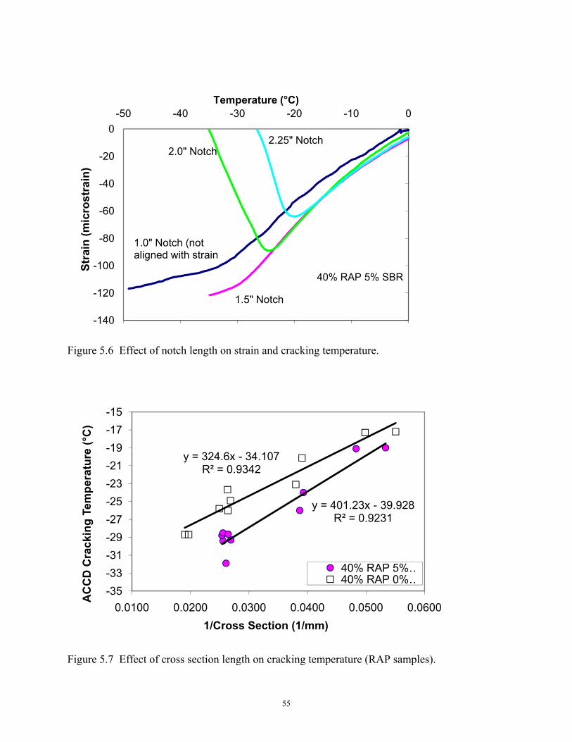
55

Figure 5.6 Effect of notch length on strain and cracking temperature.

Figure 5.7 Effect of cross section length on cracking temperature (RAP samples).

-140

-120

-100

-80

-60

-40

-20

0-50 -40 -30 -20 -10 0

Stra

in (m

icro

stra

in)

Temperature (°C)

40% RAP 5% SBR

2.25" Notch2.0" Notch

1.5" Notch

1.0" Notch (not aligned with strain

y = 401.23x - 39.928R² = 0.9231

y = 324.6x - 34.107R² = 0.9342

-35-33-31-29-27-25-23-21-19-17-15

0.0100 0.0200 0.0300 0.0400 0.0500 0.0600

AC

CD

Cra

ckin

g Te

mpe

ratu

re (°

C)

1/Cross Section (1/mm)

40% RAP 5% …40% RAP 0% …

56

Figure 5.8 Effect of cross section length on cracking temperatures of AAA-1 and AAC-1 mixes.

Performing all of the four notch length tests was time consuming. The 38.1 mm (1.5 in.)

cross section was chosen as a standard notch length for the ACCD test. This notch length was a

compromise between keeping an adequate dimension and keeping the notch long enough to

prevent many transitional failures as observed with the 40% RAP 5% SBR mix. Thus, all

following samples tested were of a 38.1 mm (1.5 in.) cross section.

5.4 Finalized ACCD Test Procedure and Determination of Cracking Temperature.

This section will present only a brief description of the test procedure. For a detailed

description refer to Appendix B (Section B.1).

First, the apparatus is cleaned with kerosene to remove all asphalt binder bonded to the

Invar and aluminum rings. Prior to the day of testing, two pans of approximately 3000g of loose

y = 276.37x - 44.399R² = 0.9787

y = 110.37x - 36.788R² = 0.7916

-40

-38

-36

-34

-32

-30

0.010 0.020 0.030 0.040 0.050 0.060

Cra

ckin

g Te

mep

ratu

re (°

C)

1/Cross Section (1/mm)

AAA-1AAC-1

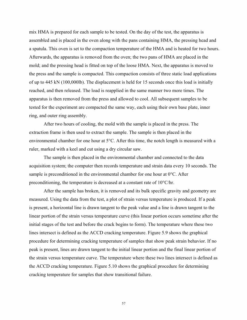
57

mix HMA is prepared for each sample to be tested. On the day of the test, the apparatus is

assembled and is placed in the oven along with the pans containing HMA, the pressing head and

a spatula. This oven is set to the compaction temperature of the HMA and is heated for two hours.

Afterwards, the apparatus is removed from the oven; the two pans of HMA are placed in the

mold; and the pressing head is fitted on top of the loose HMA. Next, the apparatus is moved to

the press and the sample is compacted. This compaction consists of three static load applications

of up to 445 kN (100,000lb). The displacement is held for 15 seconds once this load is initially

reached, and then released. The load is reapplied in the same manner two more times. The

apparatus is then removed from the press and allowed to cool. All subsequent samples to be

tested for the experiment are compacted the same way, each using their own base plate, inner

ring, and outer ring assembly.

After two hours of cooling, the mold with the sample is placed in the press. The

extraction frame is then used to extract the sample. The sample is then placed in the

environmental chamber for one hour at 5°C. After this time, the notch length is measured with a

ruler, marked with a keel and cut using a dry circular saw.

The sample is then placed in the environmental chamber and connected to the data

acquisition system; the computer then records temperature and strain data every 10 seconds. The

sample is preconditioned in the environmental chamber for one hour at 0°C. After

preconditioning, the temperature is decreased at a constant rate of 10°C/hr.

After the sample has broken, it is removed and its bulk specific gravity and geometry are

measured. Using the data from the test, a plot of strain versus temperature is produced. If a peak

is present, a horizontal line is drawn tangent to the peak value and a line is drawn tangent to the

linear portion of the strain versus temperature curve (this linear portion occurs sometime after the

initial stages of the test and before the crack begins to form). The temperature where these two

lines intersect is defined as the ACCD cracking temperature. Figure 5.9 shows the graphical

procedure for determining cracking temperature of samples that show peak strain behavior. If no

peak is present, lines are drawn tangent to the initial linear portion and the final linear portion of

the strain versus temperature curve. The temperature where these two lines intersect is defined as

the ACCD cracking temperature. Figure 5.10 shows the graphical procedure for determining

cracking temperature for samples that show transitional failure.

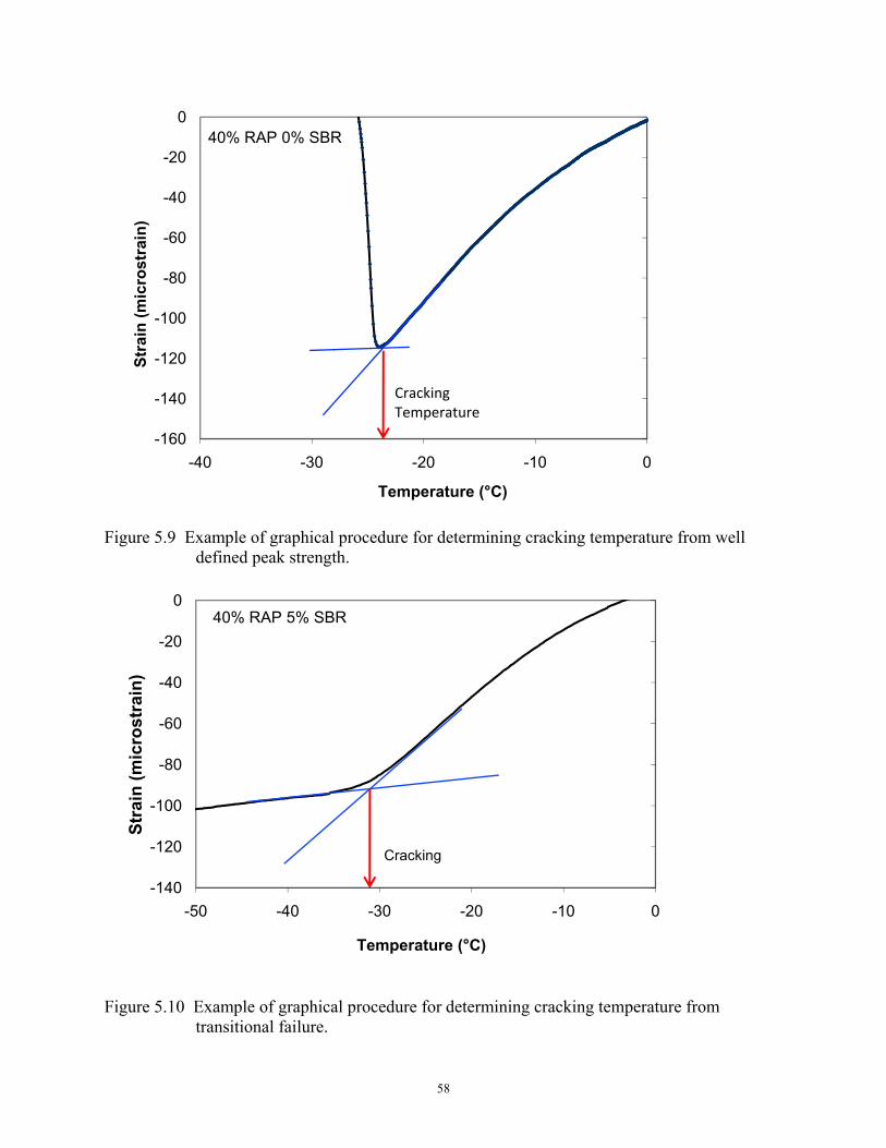
58

Figure 5.9 Example of graphical procedure for determining cracking temperature from well

defined peak strength.

Figure 5.10 Example of graphical procedure for determining cracking temperature from

transitional failure.

-160

-140

-120

-100

-80

-60

-40

-20

0

-40 -30 -20 -10 0

Stra

in (m

icro

stra

in)

Temperature (°C)

40% RAP 0% SBR

Cracking Temperature

-140

-120

-100

-80

-60

-40

-20

0

-50 -40 -30 -20 -10 0

Stra

in (m

icro

stra

in)

Temperature (°C)

40% RAP 5% SBR

Cracking

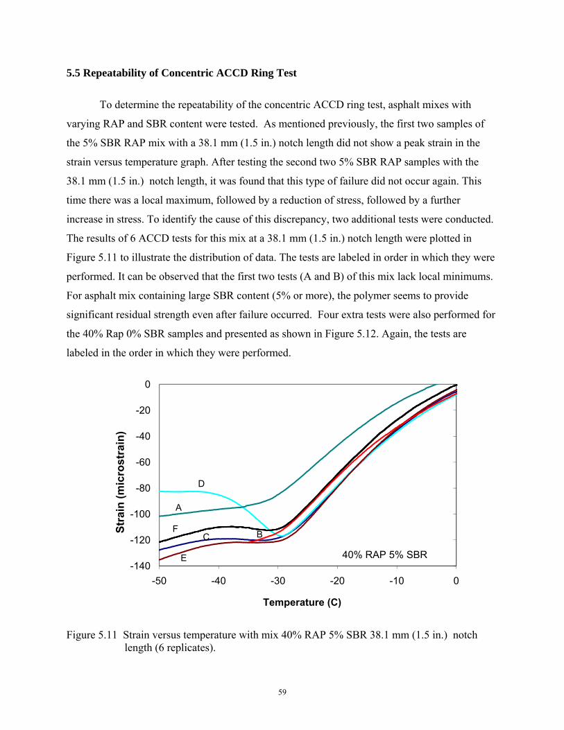
59

5.5 Repeatability of Concentric ACCD Ring Test

To determine the repeatability of the concentric ACCD ring test, asphalt mixes with

varying RAP and SBR content were tested. As mentioned previously, the first two samples of

the 5% SBR RAP mix with a 38.1 mm (1.5 in.) notch length did not show a peak strain in the

strain versus temperature graph. After testing the second two 5% SBR RAP samples with the

38.1 mm (1.5 in.) notch length, it was found that this type of failure did not occur again. This

time there was a local maximum, followed by a reduction of stress, followed by a further

increase in stress. To identify the cause of this discrepancy, two additional tests were conducted.

The results of 6 ACCD tests for this mix at a 38.1 mm (1.5 in.) notch length were plotted in

Figure 5.11 to illustrate the distribution of data. The tests are labeled in order in which they were

performed. It can be observed that the first two tests (A and B) of this mix lack local minimums.

For asphalt mix containing large SBR content (5% or more), the polymer seems to provide

significant residual strength even after failure occurred. Four extra tests were also performed for

the 40% Rap 0% SBR samples and presented as shown in Figure 5.12. Again, the tests are

labeled in the order in which they were performed.

Figure 5.11 Strain versus temperature with mix 40% RAP 5% SBR 38.1 mm (1.5 in.) notch

length (6 replicates).

-140

-120

-100

-80

-60

-40

-20

0

-50 -40 -30 -20 -10 0

Stra

in (m

icro

stra

in)

Temperature (C)

40% RAP 5% SBR

D

A

FC

E

B

60

Figure 5.12 Strain versus temperature with mix 40% RAP 0% SBR 38.1 mm (1.5 in.) notch

length (6 replicates)

When compared with the 5% SBR RAP results, the 0% SBR RAP behavior is quite

different. The heavily modified mix exhibited more ductile or transient failure with stresses

continuing to increase while the unmodified mix exhibited more brittle behavior with the stresses

returning to zero. This confirms the previous research by Hesp et al., (2000) which suggested

that polymer modification of binders may help prevent catastrophic failure during low

temperature thermal cracking. The results of ACCD tests for all RAP samples are presented in

Table 5.1. The average ACCD cracking temperatures for samples with the 38.1 mm (1.5 in.)

cross section are presented in Table 5.2.

-160

-140

-120

-100

-80

-60

-40

-20

0

-70 -60 -50 -40 -30 -20 -10 0

Stra

in (m

icro

stra

in)

Temperature (°C)

40% RAP 0% SBR A

B

D

F

CE

61

Table 5.1 ACCD Results of RAP Mixes.

 Cross Section

Length  

Cracking temperature

(°C) 

 Strain (με) 

Fracture Area   % Air Voids (in) (mm) (in2) (mm2)

40% RAP 5% SBR 0.738 18.7 -19.0 -75.7 na na 5.5

40% RAP 5% SBR 0.815 20.7 -19.1 -63.1 na na na

40% RAP 5% SBR 1.018 25.9 -26.0 -92.5 na na 6.2

40% RAP 5% SBR 1.002 25.5 -24.0 -88.6 na na 6.2

40% RAP 5% SBR 1.51 38.4 -31.9 -120.6 na na 5.7

40% RAP 5% SBR 1.54 39.1 -29.4 -112.7 na na 5.5

40% RAP 5% SBR 2.042 51.9 na na na na 5.6

40% RAP 5% SBR na na na na na 9.0

40% RAP 4% SBR 1.464 37.2 -27.0 -120.6 3.62 2335 5.8

40% RAP 4% SBR 1.492 37.9 -25.6 -117 3.72 2400 5.6

40% RAP 4% SBR 1.487 37.8 -25.5 -118.9 3.70 2387 6.4

40% RAP 3% SBR 1.53 38.9 -27.2 -134.5 3.86 2490 5.0

40% RAP 3% SBR 1.512 38.4 -26.2 -141.3 3.73 2406 4.7

40% RAP 3% SBR 1.444 36.7 -25.4 -114.1 3.57 2303 4.6

40% RAP 3% SBR 1.451 36.9 -26.0 -139.1 3.59 2316 4.7

40% RAP 0% SBR 0.79 20.1 -17.3 -119.6 na na 5.5

40% RAP 0% SBR 0.715 18.2 -17.2 -70.4 na na na

40% RAP 0% SBR 1.036 26.3 -23.1 -129.9 na na 6.2

40% RAP 0% SBR 1.008 25.6 -20.1 -88.4 na na 4.4

40% RAP 0% SBR 1.491 37.9 -26.0 -147 na na 4.6

40% RAP 0% SBR 1.58 40.1 -25.8 -90.3 na na 4.7

40% RAP 0% SBR 1.5 38.1 -26.5 -123.6 na na na

40% RAP 0% SBR 1.5 38.1 -25.4 -88 na na na

40% RAP 0% SBR 1.495 38.0 -23.7 -113.7 3.36 2168 5.0

40% RAP 0% SBR 1.467 37.3 -24.9 -126.3 3.57 2303 4.6

40% RAP 0% SBR 2.0 50.8 -28.7 -139.3 na na 4.4

40% RAP 0% SBR 2.07 52.6 -28.7 -141.5 na na 4.6

20% RAP 0% SBR 1.508 38.3 -25.3 -117.6 3.74 2413 7.0

20% RAP 0% SBR 1.513 38.4 -26.6 -124.5 3.80 2452 6.8

20% RAP 0% SBR 1.5 38.1 -25.4 -98.9 3.79 2445 6.8

20% RAP 0% SBR 1.534 39.0 -25.2 -115.5 3.81 2458 6.9

40% RAP (58-22) 1.487 37.8 -29.1 -132.2 3.73 2406 5.9

40% RAP (58-22) 1.455 37.0 -27.6 -126.2 3.55 2290 6.0

40% RAP (58-22) 1.47 37.3 -27.7 -122.1 3.59 2316 6.3

40% RAP (58-22) 1.428 36.3 -27.9 -135.5 3.60 2323 6.1

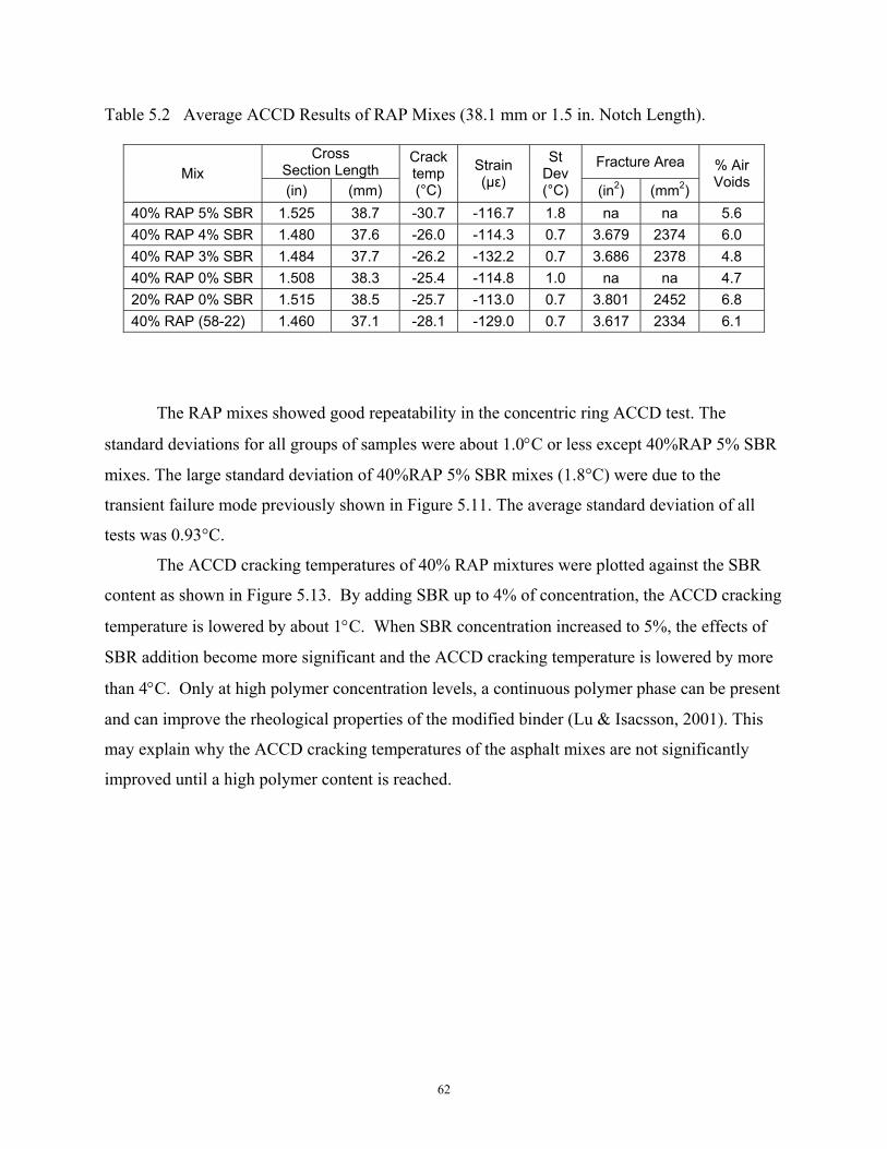
62

Table 5.2 Average ACCD Results of RAP Mixes (38.1 mm or 1.5 in. Notch Length).

Mix Cross

Section Length Crack temp (°C)

Strain (με)

St Dev (°C)

Fracture Area % Air Voids (in) (mm) (in2) (mm2)

40% RAP 5% SBR 1.525 38.7 -30.7 -116.7 1.8 na na 5.6 40% RAP 4% SBR 1.480 37.6 -26.0 -114.3 0.7 3.679 2374 6.0 40% RAP 3% SBR 1.484 37.7 -26.2 -132.2 0.7 3.686 2378 4.8 40% RAP 0% SBR 1.508 38.3 -25.4 -114.8 1.0 na na 4.7 20% RAP 0% SBR 1.515 38.5 -25.7 -113.0 0.7 3.801 2452 6.8 40% RAP (58-22) 1.460 37.1 -28.1 -129.0 0.7 3.617 2334 6.1

The RAP mixes showed good repeatability in the concentric ring ACCD test. The

standard deviations for all groups of samples were about 1.0°C or less except 40%RAP 5% SBR

mixes. The large standard deviation of 40%RAP 5% SBR mixes (1.8°C) were due to the

transient failure mode previously shown in Figure 5.11. The average standard deviation of all

tests was 0.93°C.

The ACCD cracking temperatures of 40% RAP mixtures were plotted against the SBR

content as shown in Figure 5.13. By adding SBR up to 4% of concentration, the ACCD cracking

temperature is lowered by about 1°C. When SBR concentration increased to 5%, the effects of

SBR addition become more significant and the ACCD cracking temperature is lowered by more

than 4°C. Only at high polymer concentration levels, a continuous polymer phase can be present

and can improve the rheological properties of the modified binder (Lu & Isacsson, 2001). This

may explain why the ACCD cracking temperatures of the asphalt mixes are not significantly

improved until a high polymer content is reached.

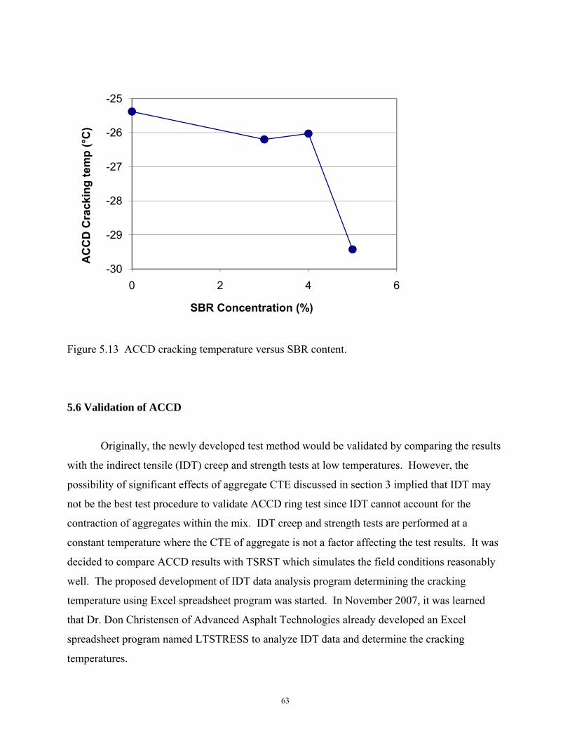
63

Figure 5.13 ACCD cracking temperature versus SBR content.

5.6 Validation of ACCD

Originally, the newly developed test method would be validated by comparing the results

with the indirect tensile (IDT) creep and strength tests at low temperatures. However, the

possibility of significant effects of aggregate CTE discussed in section 3 implied that IDT may

not be the best test procedure to validate ACCD ring test since IDT cannot account for the

contraction of aggregates within the mix. IDT creep and strength tests are performed at a

constant temperature where the CTE of aggregate is not a factor affecting the test results. It was

decided to compare ACCD results with TSRST which simulates the field conditions reasonably

well. The proposed development of IDT data analysis program determining the cracking

temperature using Excel spreadsheet program was started. In November 2007, it was learned

that Dr. Don Christensen of Advanced Asphalt Technologies already developed an Excel

spreadsheet program named LTSTRESS to analyze IDT data and determine the cracking

temperatures.

-30

-29

-28

-27

-26

-25

0 2 4 6

AC

CD

Cra

ckin

g te

mp

(°C

)

SBR Concentration (%)

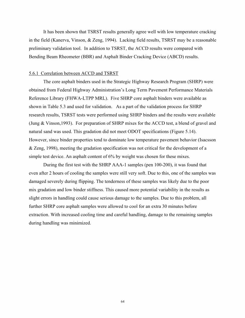
64

It has been shown that TSRST results generally agree well with low temperature cracking

in the field (Kanerva, Vinson, & Zeng, 1994). Lacking field results, TSRST may be a reasonable

preliminary validation tool. In addition to TSRST, the ACCD results were compared with

Bending Beam Rheometer (BBR) and Asphalt Binder Cracking Device (ABCD) results.

5.6.1 Correlation between ACCD and TSRST

The core asphalt binders used in the Strategic Highway Research Program (SHRP) were

obtained from Federal Highway Administration’s Long Term Pavement Performance Materials

Reference Library (FHWA-LTPP MRL). Five SHRP core asphalt binders were available as

shown in Table 5.3 and used for validation. As a part of the validation process for SHRP

research results, TSRST tests were performed using SHRP binders and the results were available

(Jung & Vinson,1993). For preparation of SHRP mixes for the ACCD test, a blend of gravel and

natural sand was used. This gradation did not meet ODOT specifications (Figure 5.14).

However, since binder properties tend to dominate low temperature pavement behavior (Isacsson

& Zeng, 1998), meeting the gradation specification was not critical for the development of a

simple test device. An asphalt content of 6% by weight was chosen for these mixes.

During the first test with the SHRP AAA-1 samples (pen 100-200), it was found that

even after 2 hours of cooling the samples were still very soft. Due to this, one of the samples was

damaged severely during flipping. The tenderness of these samples was likely due to the poor

mix gradation and low binder stiffness. This caused more potential variability in the results as

slight errors in handling could cause serious damage to the samples. Due to this problem, all

further SHRP core asphalt samples were allowed to cool for an extra 30 minutes before

extraction. With increased cooling time and careful handling, damage to the remaining samples

during handling was minimized.

65

Table 5.3 Five SHRP Core Asphalt Used in ACCD Validation.

(a Mortazavi & Moulthrop, 1993; b Jung & Vinson,1993)

Figure 5.14 Aggregate gradation for the SHRP core asphalt mixes.

1912.5

9.5

4.75

2.36

1.18

0.6000.3000.1500.075

0102030405060708090

100

Perc

ent P

assi

ng

Sieve Size, mm

0.45 Power Chart (12.5mm NMS)

ODOT SpecGravel-Sand Blend

Binder Source Viscosity/Penn Grade

Critical Temp (°C) AASHTO

M320 Table 1a

ABCD TSRSTb

AAA-1 Lloydminster 150/200 -32.8 -36.5 -30.3

AAB-1 Wyoming High Sulfur AC-10 -24.4 -31.9 -25.4

AAC-1 Redwater AC-8 -20.0 -32.3 -22.5

AAF-1 West Texas Sour AC-20 NA -24.6 -16.9

AAM-1 West Texas Intermediate AC-20 -10.0 -29.1 -21.0

66

Table 5.4 summarizes the results from ACCD ring test. The averages of the data from

samples with notch lengths of 38.1 mm (1.5 in.) were given in Table 5.5 and used to compare

with TSRST results as shown in Figure 5.15. The standard deviation for ACCD tests on SHRP

binders ranges from 0.1°C to 1.4°C (average 0.85°C). This is comparable to the standard

deviations of the TSRST which range between 0.53-1.2°C (Isacsson & Zeng, 1998). The ACCD

cracking temperature correlates well with TSRST cracking temperature with coefficient of

determination (r2) of 0.86. The ACCD cracking temperatures are generally colder than the

TSRST temperatures.

Table 5.4 ACCD Results of SHRP Binder Mixes.

Mix Cross Section

Length Cracking

temp (°C)

Peak Strain (με)

Fracture Area % Air Voids (in) (mm) (in2) (mm2)

AAA-1 1.593 40.5 -38.4 -91.1 4.077 2630 11.8 AAA-1 1.571 39.9 -36.8 -76.8 3.922 2530 10.2 AAA-1 1.070 27.2 -34.1 -60.6 2.617 1688 11.4 AAA-1 0.748 19.0 -29.9 -47.7 1.813 1170 10.8 AAB-1 1.439 36.6 -34.2 -80.8 3.568 2302 10.6 AAB-1 1.583 40.2 -32.2 -72.4 3.791 2446 11.4 AAC-1 1.529 38.8 -33.6 -65.6 3.708 2392 10.9 AAC-1 1.537 39.0 -34.3 -74.0 3.742 2414 10.8 AAC-1 1.089 27.7 -32.8 -61.4 2.718 1754 11.7 AAF-1 1.491 37.9 -26.3 -27.1 3.727 2405 11.1 AAF-1 1.452 36.9 -27.9 -29.3 3.626 2339 11.5 AAM-1 1.451 36.9 -29.5 -96.1 3.550 2290 na AAM-1 1.472 37.4 -29.4 -69.2 3.414 2203 10.5

67

Table 5.5 Average ACCD Results of SHRP Binder Mixes.

Mix Cross Section

Length  Crack temp (°C)

Peak Strain (με)

St Dev (°C)

Fracture Area% Air Voids (in) (mm) (in2) (mm2)

AAA-1 1.582 40.2  -37.6 -83.6 1.1 4.000 2581  11.0 AAB-1 1.511 38.4  -33.2 -74.9 1.4 3.680 2374  11.0 AAC-1 1.533 38.9  -34.0 -68.8 0.5 3.725 2403  10.9 AAF-1 1.471 37.4  -27.1 -74.3 1.1 3.676 2372  11.3 AAM-1 1.461 37.1  -29.5 -81.5 0.1 3.482 2246  10.5

Figure 5.15 ACCD versus TSRST* cracking temperatures for SHRP binders. *TSRST Data from: Jung & Vinson (1993).

y = 0.7291x - 14.493R² = 0.8674

-40

-38

-36

-34

-32

-30

-28

-26

-35 -30 -25 -20 -15

AC

CD

Cra

ckin

g Te

mp

(°C

)

TSRST Cracking Temperature (°C)

AAC‐1 Mix

68

5.6.2 Correlation between ACCD and Bending Beam Rheometer (BBR)

Previous research has shown BBR data to correlate to TSRST data (King et al., 1993;

Epps, 1998). Since both ACCD and BBR data correlate to TSRST, it was expected that they

would correlate with one another. In order to verify this, the stiffness and m-values at different

temperatures were taken from the SHRP materials library (Mortazavi & Moulthrop, 1993) for

each binder. With this information critical temperatures for AAA-1, AAB-1, AAC-1 and AAM-1

were calculated as given in Table 5.3. The data for AAF-1 in the SHRP materials library was not

sufficient to determine this temperature. The ACCD cracking temperature was then plotted

versus the BBR critical temperatures for each SHRP core asphalt. This showed that ACCD did

correlate with BBR tests with a coefficient of determination of 0.88 (refer to Figure 5.16)

Figure 5.16 ACCD cracking temperature versus BBR critical temperature for SHRP binders.

y = 0.3381x - 26.18R² = 0.9195

-40

-38

-36

-34

-32

-30

-28

-35 -30 -25 -20 -15 -10

AC

CD

Cra

ckin

g Te

mp

(°C

)

BBR Critical Temperature (°C)

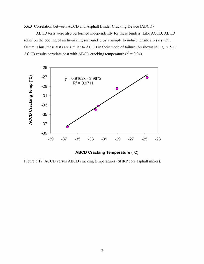
69

5.6.3 Correlation between ACCD and Asphalt Binder Cracking Device (ABCD)

ABCD tests were also performed independently for these binders. Like ACCD, ABCD

relies on the cooling of an Invar ring surrounded by a sample to induce tensile stresses until

failure. Thus, these tests are similar to ACCD in their mode of failure. As shown in Figure 5.17

ACCD results correlate best with ABCD cracking temperature (r2 = 0.94).

Figure 5.17 ACCD versus ABCD cracking temperatures (SHRP core asphalt mixes).

y = 0.9162x - 3.9672R² = 0.9711

-39

-37

-35

-33

-31

-29

-27

-25

-39 -37 -35 -33 -31 -29 -27 -25 -23

AC

CD

Cra

ckin

g Te

mp

(°C

)

ABCD Cracking Temperature (°C)

70

5.7 ACCD Results of Ohio DOT Mixes

In order to allow for future validation of the ACCD test method using field results, large

quantities of four loose asphalt mixes were obtained from the Ohio Department of Transportation.

These mixes were placed on actual roadways during the 2007 season. These mixes were labeled

OD-1, OD-2, OD-3 and OD-4. More information about these mixes is included in Appendix C.

Four tests were performed for each of these mixes. Only two samples were discarded in the

entire 16 sample set, both due to operator errors during testing. The results of this testing are

presented in Table 5.6 and the average values for each mix are presented in Table 5.7. The

ACCD cracking temperatures for the ODOT mixes showed good repeatability. The highest

standard deviation was 0.7°C and the average standard deviation was 0.44°C.

Even though four binders were graded to the same low temperature performance level

(PG -22), their ACCD cracking temperatures were significantly different. Mixes with binders

containing SBS polymer showed 2-7°C lower cracking temperature than the mixes with no

polymer (OD-2).

The ACCD cracking temperatures of the binders used in ODOT mixes were also

compared to their binders’ BBR critical temperatures. The results are presented in this Figure

5.18. The ACCD cracking temperatures showed good correlation to BBR results. However,

mixes prepared with different aggregates may result in different ACCD versus BBR results.

71

Table 5.6 ACCD Results of ODOT Mixes.

Mix Cross Section

Length  Cracking temp (°C)

Strain (με)

Fracture Area% Air Voids   (in) (mm) (in2) (mm2)

OD-1 (PG 70-22 SBS) 1.491 37.9 -28.6 -92.9 3.662 2363 7.4 OD-1 (PG 70-22 SBS) 1.497 38.0 -28.7 -100.6 3.624 2338 7.4 OD-1 (PG 70-22 SBS) 1.489 37.8 -28.8 -106.4 3.642 2350 7.5 OD-2 (PG 64-22) 1.560 39.6 -26.3 -116.2 3.961 2555 4.8 OD-2 (PG 64-22) 1.532 38.9 -27.1 -136.6 3.709 2393 4.7 OD-2 (PG 64-22) 1.466 37.2 -26.6 -118.8 3.614 2332 4.6 OD-2 (PG 64-22) 1.437 36.5 -27.9 -121.5 3.603 2325 4.8 OD-3 (PG 76-22 SBS) 1.503 38.2 -29.7 -137.8 3.586 2314 5.9 OD-3 (PG 76-22 SBS) 1.505 38.2 -29.3 -145.0 3.940 2542 5.8 OD-3 (PG 76-22 SBS) 1.500 38.1 -29.5 -143.7 3.554 2293 5.6 OD-3 (PG 76-22 SBS) 1.591 40.4 -30.2 -158.3 3.815 2461 5.6 OD-4 (PG 70-22 SBS) 1.537 39.0 -34.6 -137.7 3.790 2445 7.6 OD-4 (PG 70-22 SBS) 1.510 38.4 -33.8 -113.9 3.743 2415 7.6 OD-4 (PG 70-22 SBS) 1.489 37.8 -33.4 -131.2 3.504 2261 7.3

ODOT Results

Table 5.7 Average ACCD Results of ODOT Mixes.

Mix

Cross Section Length

Cracking

temp (°C)

Strain (μe)

St Dev (°C)

Fracture Area % Air Voids (in) (mm) (in2) (mm2)

OD-1 (PG 70-22 SBS) 1.492 37.9 -28.7 -100.0 0.1 3.642 2350 7.4 OD-2 (PG 64-22) 1.499 38.1 -26.9 -123.3 0.7 3.722 2401 4.7 OD-3 (PG 76-22 SBS) 1.525 38.7 -29.7 -146.2 0.4 3.724 2403 5.7 OD-4 (PG 70-22 SBS) 1.512 38.4 -33.9 -127.6 0.6 3.679 2374 7.5

72

Figure 5.18 ACCD cracking temperature versus BBR critical temperature (ODOT mixes).

5.8 Effects of Variations in ACCD sample Geometry

Previous experience with RAP samples had shown that variation in notch length had an

effect on cracking temperature. It is unknown to what extent variation in sample height from

sample to sample would affect the results for a given notch length. For this reason, efforts were

made to maintain a consistent sample height. However, some samples did show considerable

variability in height (up to 5.1 mm or 0.2 in.) from one side of the outer diameter to the other. It

may be possible that variations in the cross section due to errors in sawing combined with the

errors due to sample heights would introduce some variability into the cracking results. Increased

fracture area may lead to higher fracture resistance, and therefore lower cracking temperature.

The cracking temperature versus cracking area is shown in Figure 5.19. There is no significant

effect on the ACCD cracking temperature by uneven specimen geometry tested (226 – 2581 mm2

or 0.35-4.0 in2).

y = 1.5453x + 8.9033R² = 0.9482

y = 0.3381x - 26.18R² = 0.8735

-40

-35

-30

-25

-20

-35 -30 -25 -20 -15 -10 -5

AC

CD

Cra

ckin

g Te

mp

(°C

)

BBR Critical Temp (°C)

ODOT MixSHRP Mix

73

Figure 5.19 ACCD cracking temperature versus fracture area (ODOT samples).

-40

-35

-30

-25

-20

2200 2300 2400 2500 2600

AC

CD

Cra

ckin

g Te

mp

(°C

)

Fracture Area (mm2)

OD-1 OD-2 OD-3 OD-4

74

6. FINITE ELEMENT ANALYSIS

In order to validate the test methods and to visualize the stress distributions present in the

samples, finite element modeling was used. Using the finite element computer software

ABAQUS, the samples for both the fixed frame and the concentric ring ACCD tests were

modeled. For simplicity, the HMA samples were assumed to be elastic, homogenous and

isotropic. Assuming HMA is a homogeneous and isotropic material does place limitations on the

usefulness of the results. However, the availability of suitable data was the major factor

preventing a more rigorous analysis. Since this analysis was only to approximate the stress

distributions within the samples, these assumptions would not invalidate the usefulness of this

phase of the investigation. Furthermore, the assumption of elasticity is reasonable for HMA at

cold temperatures, where the modulus of the binder approaches a constant value, the glassy

modulus. Thus, the results of this analysis do provide useful information about the stress

distributions within the ACCD samples.

The important parameters needed to complete this analysis were the elastic modulus of

Invar steel, the elastic modulus of HMA, the Poisson’s ratio of Invar, the Poisson’s ratio of HMA,

the dimensions of the Invar, the dimensions of the specimen, and the strain in the Invar during a

typical test. The elastic modulus and Poisson’s ratio of Invar are approximately 141 GPa (20,500

ksi) and 0.29 respectively. The glassy shear modulus of 1 GPa (145 ksi) and a Poisson’s ratio of

0.2 were good estimates for modeling HMA (Christensen, & Anderson, 1992). Thus, the values

of 2.4 GPa (348 ksi) and 0.2 were used for Young’s modulus and Poisson’s ratio for all of the

analyses in this section. An element size of approximately 5 mm (0.20 inch) was used for this

analysis.

6.1 Cylindrical Sample Epoxied to a Fixed Frame

The fixed frame ACCD was analyzed first. The specimen was modeled as a cylinder

70.6mm (2.78 inch) in diameter and 100 mm (3.94 inch) in height. Due to symmetry, only half of

the sample was modeled. This produced a cylinder 70.6 mm (2.78 in.) in diameter and 50 mm

(1.97 in.) in height. To simulate the epoxied end, one of the ends of the model was completely

75

fixed. No displacement or rotation was allowed in any direction at this end. Next, the load was

calculated using the strain in the Invar rods measured from actual tests. At fracture during the

fixed frame test, a strain jump of 50με was typical for all three of the rods. This strain is

equivalent to approximately 10.7 kN (2,405 lb) load in the test sample. Dividing by the cross

section of the sample produced a stress of approximately 2.76 MPa (400 psi). Figure 6.1 shows

the assumed behavior of the fixed frame test for calculating the stresses within the sample. Using

these values the analysis was conducted. Since cracking in HMA at low temperature is

considered to be brittle in nature, the maximum principle stress failure criterion is appropriate.

The results of this analysis are shown in Figure 6.2. Areas of high stress are present at the end

due to its restrained condition by epoxy, which prevented contraction in the diametral direction.

The highest stress is present in the outer surface of the sample at the fixed end while the lowest

stress is in the center of the sample at the fixed end. This stress concentration at the end supports

the fact that samples tested with this setup usually failed near the end.

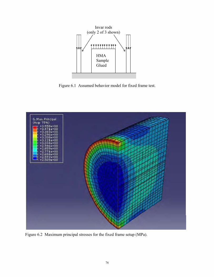
76

Figure 6.1 Assumed behavior model for fixed frame test.

Figure 6.2 Maximum principal stresses for the fixed frame setup (MPa).

HMA Sample Glued

Invar rods (only 2 of 3 shown)

77

6.2 Concentric Ring Apparatus

Subsequently, a series of models were developed to evaluate the effect of notch length on

the concentric ring ACCD. Each of these samples was modeled as a 254 mm (10 in.) outer

diameter, 101.6 mm (4 in.) inner diameter ring with a height of 63.5 mm (2.5 in.). Due to

symmetry only half of the ring was modeled. For this analysis, it was assumed that as the HMA

contracted, the Invar ring would exert a uniform pressure on the sample and would experience a

uniform strain. Figure 6.3 shows the assumed stress distribution in the concentric ring ACCD

during testing, while Figure 6.4 shows the model used for the finite element analysis. To obtain

the magnitude of the uniform pressure for each notch length, actual strain measurements from

validation tests were used. Since the cross sectional area of the Invar steel was known, the force

applied to the ring was calculated by multiplying the measured strain by the elastic modulus of

the Invar steel and the cross sectional area. This force was then divided by the area of the sample

to yield the average stress developed in the sample. These pressures were calculated to be as

follows: 1.8MPa, 2.3 MPa, 3.2 MPa, 3.9 MPa and 5.6 MPa for the samples with 19.1 mm (0.75

in.), 25.4 mm (1 in.), 38.1 mm (1.5 in.), 50.8 mm (2 in.) and 76.2 mm (3 in.) cross sections

respectively.

However, for the 25.4 mm (1.0 in.) notch length and no notch models, the strain at failure

was not known. These strains were estimated based on a linear trend of notch length versus strain

at failure from the previous notch lengths. Thus, these values should only be used as a means to

compare the general stress distributions in the samples rather than to obtain a value for actual

stresses present. From this analysis two important facts become apparent. First, as the notch

length increased, a less uniform stress distribution around the sample diameter was observed

(Figures 6.5 to 6.9). Secondly, stress concentrations through the cracking area of the sample were

observed due to the presence of the notch. Longer notches showed greater stress concentrations.

For all notch lengths, the stress was higher at the tip of the notch. Due to this fact, it is expected

that the cracks propagate from the tip of the notch inward. The stress concentration factor was

calculated by dividing the maximum stress recorded in the analysis divided by the average stress

calculated above. The stress concentration factors for all test set-ups are presented in table 6.1.

For 38.1 mm (1.5 in.) notch, the stress concentration factor is estimated to be 3.81.

78

Figure 6.3 Assumed stress distribution in the HMA sample and Invar ring.

Figure 6.4 Model used for finite element analysis.

79

Figure 6.5 Max principal stresses in the concentric ring setup (57.2 mm or 2.25 in. notch) (MPa).

Figure 6.6 Max principal stresses for the concentric ring setup (50.8 mm or 2.0 in. notch) (MPa).

80

Figure 6.7 Max principal stresses for the concentric ring setup (38.1 mm or 1.5 in. notch) (MPa).

Figure 6.8 Max principal stresses for the concentric ring setup (25.4 mm or 1.0 in. notch) (MPa).

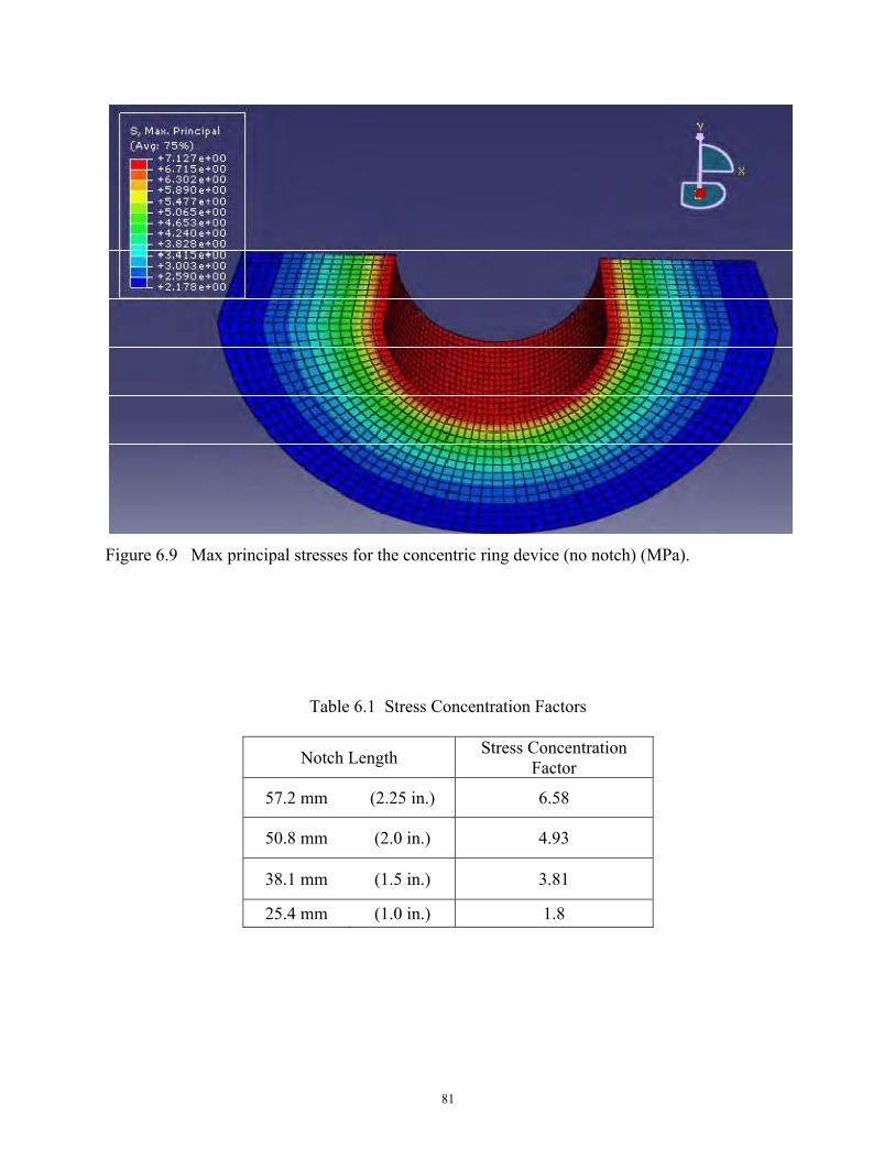
81

Figure 6.9 Max principal stresses for the concentric ring device (no notch) (MPa).

Table 6.1 Stress Concentration Factors

Notch Length Stress Concentration Factor

57.2 mm (2.25 in.) 6.58

50.8 mm (2.0 in.) 4.93

38.1 mm (1.5 in.) 3.81

25.4 mm (1.0 in.) 1.8

82

The results of this analysis provided useful insight to the stress distributions within the

ACCD samples. First, it explained why every sample for the fixed frame ACCD failed near one

of its ends. As suspected, end effects control the failure location of the sample and may force the

crack to occur at a warmer temperature than would occur without end effects. Second, the

analysis showed the effect of the notch length on the stress distribution within the concentric ring

ACCD sample. As the notch length increases, the stress concentration at the fracture area

becomes larger. Given the stress distributions observed, it is believed that the 38.1 mm (1.5 in.)

notch length may be a good choice for use as the standard cross section width. This notch length

provides a reasonable compromise between stress distributions and sample geometry due to

aggregate size limitations. This analysis also indicates that the stresses are highest at the tip of

the notch. Thus, the cracks in the sample would likely initiate at the tip of the notch and progress

inwards.

83

7. CONCLUSIONS AND RECOMMENDATIONS

7.1 Conclusions

A simple test device, named the Asphalt Concrete Cracking Device (ACCD), was

successfully developed to measure the low temperature cracking resistance of HMA and was

validated using laboratory tests. Four Ohio DOT asphalt mixes used during 2007 construction

season were tested with ACCD for future field validation. Using the strain gage technique, the

CTE of 14 Ohio aggregates collected from 9 Ohio DOT Districts were also determined. This

study is summarized with the following conclusions.

• Of 14 Ohio aggregates studied, the maximum and the minimum CTEs are 11.4 and 4.0 x

10-6/°C, respectively and are similar to previously reported values for aggregate CTE.

• Orthotropic and composite nature of asphalt pavement contraction during cooling makes

the effects of aggregate CTE important in low temperature thermal cracking of asphalt

pavement. For asphalt mixes of similar CTE, one made of aggregate with large CTE

may develop 36% more thermally induced strain (or stress) in asphalt binder in the mix

than another mix with low CTE aggregate.

• The concentric ring ACCD test for evaluating low temperature cracking potential of

asphalt pavement is successfully developed through this project. The ACCD test is

repeatable. For the various mixes tested, standard deviations were typically less than 1°C,

with 0.78°C average.

• The ACCD test results were indirectly validated by comparing with TSRST test results.

The ACCD cracking temperatures of 5 mixes with SHRP core asphalt binder correlate

well with the TSRST results of mixes prepared with the same binders but with different

aggregate (r2 =0.86).

• ACCD test is a simpler and faster test method than the current TSRST. The ACCD test

does not require the time consuming trimming and gluing processes needed in the

TSRST procedure. If specimen curing is not required prior to the test, four ACCD

samples can be prepared and tested in an 8 hour-day.

84

• In the ACCD test, since the test specimen is compacted with the ACCD ring and remains

with the ring during the test, the alignment problem in the TSRST procedure is very

unlikely.

• ACCD was sensitive to the effects of SBR concentration in RAP mixes. At a high SBR

content (5% by weight), a significant improvement in the low temperature performance

of the HMA mixes was observed while at 3% and 4% SBR concentrations, the

improvement was much smaller.

• Four Ohio DOT mixes were tested with ACCD for future field validation.

• The ACCD cracking temperatures of mixes also correlate well with the BBR critical

temperatures of binders (r2 = 0.88 for SHRP mixes prepared with single aggregate and

0.95 Ohio DOT mixes, respectively).

• The length of the notch (38.1 mm or 1.5 in.) was decided to be used in ACCD test. The

finite element analysis indicates that the stress concentration factor at the tip of the notch

was 3.81 during the test.

7.2 Recommendations for Further Research

Based on the results of this study, the following recommendations are made for the

possible future research.

• Develop improved sample compaction equipment and a procedure to minimize non-

uniformity in thickness and air voids.

• Validate the ACCD with field performance data.

• Use the ACCD to determine if physical hardening is a problem within mixtures.

• Use the ACCD to investigate the effects of mix properties on the low temperature

cracking of HMA.

85

8. REFERENCES

ARA (2004). Guide for Mechanistic-Empirical Design of New and Rehabilitated Pavement

Structures. Final Report. NCHRP 1-37A.

Bahia, H. U., & Anderson, D. A. (1993). Cracking of asphalt at low temperature as related to

bitumen rheology. Journal of the Association of Asphalt Paving Technologists, 62, 93-

129.

Bahia, H., Zeng, M., & Nam, K. (2000). Consideration of strain at failure and strength in

prediction of pavement thermal cracking. Journal of the Association of Asphalt Paving

Technologists, 69, 497-539.

Bouldin, M. G., Dongre, R., Rowe, G. M., Sharrock, M. J., & Anderson, D.A. (2000). Predicting

thermal cracking of pavements from binder properties: Theoretical basis and field

validation. Journal of the Association of Asphalt Paving Technologists, 69, 455-496.

Chehab, G. R., Kim, Y. R., Witcak, M. W., & Bonaquist, R. (2004). Prediction of thermal

cracking behavior of asphalt concrete using the viscoelastoplastic continuum damage

model. Transportation Research Record 83rd Annual Meeting. Transportation Research

Board, Washington, D.C.

Chehab, G. R., O'Quinn, E., & Kim, Y. R. (2000). Specimen geometry study for direct tension

test based on mechanical tests and air void variation in asphalt concrete specimens

compacted by Superpave Gyratory Compactor. Transportation Research Record, 1723,

125-132.

Christensen, D. W. & Anderson, D. A. (1992). Interpretation of dynamic mechanical test data for

paving grade asphalt. Journal of the Association of Asphalt Paving Technologists, 61, 67-

116.

Diefenderfer, B. K., Al-Qadi, I. L., and Reubush, S. D. (2002). "Prediction of daily temperature

profile in flexible pavements." Transportation Research Board 81st Annual Meeting

(CD-ROM), Transportation Research Board, Washington, D.C.

Epps, A. L. (1998). A comparison of measured and predicted low temperature cracking

conditions. Journal of the Association of Asphalt Paving Technologists, 67, 277- 293.

86

Fabb, T. R. J. (1974). The influence of mix composition, binder properties, and cooling rate on

AC at low temperature. Journal of the Association of Asphalt Paving Technologists, 43,

285-331.

Goodrich, J. L. (1991). Asphaltic binder rheology, asphalt concrete rheology and asphalt

concrete mix properties. Journal of the Association of Asphalt Paving Technologists, 60,

80-116.

Haas, R. C. G. & Phang, W. A. (1988). Relationships between mix characteristics and low

temperature pavement cracking. Journal of the Association of Asphalt Paving

Technologists, 57, 290-319.

Haas, R., Meyer, F., Assaf, G., & Lee, H. (1987). A comprehensive study of cold climate airport

pavement cracking. Journal of the Association of Asphalt Paving Technologists, 56, 198-

245.

Halladay, M. (1998). The Strategic Highway Research Program: An investment that has paid off.

Retrieved Apr. 9, 2008, from http://www.tfhrc.gov/pubrds/marapr98/shrp.htm

Hesp, S. A. M., Terlouw, T., & Vonk, W. C. (2000). Low temperature performance of SBS-

modified asphalt mixes. Journal of the Association of Asphalt Paving Technologists, 69,

540-573.

Iliuta, S., Hesp, S., Marasteanu, M. O., Masliwec, T., & Tam, K., K. (2004). Field validation

study of low-temperature performance grading tests for asphalt binders. Transportation

Research Record, 1875, 14-21.

Isacsson, U. & Zeng, H. (1997). Relationship between bitumen chemistry and low temperature

behavior of asphalt. Construction and Building Materials, 11(2), 83- 91.

Isacsson, U. & Zeng, H. (1998). Cracking of asphalt at low temperature as related to bitumen

rheology. Journal of Materials Science, 33(8), 2165-2170.

Johansson, L. S. & Isacsson, U. (1998). Effect of filler on low temperature physical hardening of

bitumen. Construction and Building Materials, 12, 463-470.

Johnson, T. C., Shahin, M. Y., Dempsey, N. J., & Ingersoll, J. (1979). Projected thermal and

load-associated distress in pavements incorporating different grades of asphalt cement.

Journal of the Association of Asphalt Paving Technologists, 48, 403-436.

Jung, D. & Vinson, T. S. (1993). Low temperature cracking resistance of asphalt concrete

mixtures. Journal of the Association of Asphalt Paving Technologists, 62, 54-87.

87

Jung, D. H., & Vinson, T. S. (1994). Low temperature cracking: test selection. (Report No.

SHRP-A-400). Strategic Highway Research Program, National Research Council

Kandhal, P. S., Dongre, R., & Malone, M. S. (1996). Prediction of low-temperature cracking of

Pennsylvania project using Superpave binder specifications. Journal of the Association of

Asphalt Paving Technologists, 65, 491-518.

Kanerva, H. K., Vinson, T. S., & Zeng, H. (1994). Low-temperature cracking: field evaluation of

the thermal stress restrained specimen test. (Report No. SHRP A- 401). Strategic

Highway Research Program, National Research Council

Kim, S. (2005). Direct Measurement of Asphalt Binder Thermal Cracking. J. of Materials in

Civil Engineering. vol 17. no 6, 632-639

Kim, S., Wysong, Z., & Kovach, J. (2006). Low temperature thermal cracking of asphalt binder

by asphalt binder cracking decive. Transportation Research Record, 1962, 28-35.

King, G. N., King, H. W., Harders, O., Arand, W., & Planche, P. (1993). Influence of asphalt

grade and polymer concentration on the low-temperature performance of polymer

modified asphalt. Journal of the Association of Asphalt Paving Technologists, 62, 1-22.

King, G., King, H., Pavlovich, R. D., Epps, A. L, & Kandhal, P. (1999). Additives in asphalt.

Journal of the Association of Asphalt Paving Technologists, 68A, 32-69.

Krishnan, J. M. & Rajagopal, K. R. (2005). On the mechanical behavior of asphalt. Mechanics of

Materials, 37(11), 1085-1100.

Lee, N. K., Morrison, G. R., & Hesp, S. A. M. (1995). Low temperature fracture of

polyethylene-modified asphalt ninders and asphalt concrete mixes. Journal of the

Association of Asphalt Paving Technologists, 64, 534-574.

Li, Xi., Zofka, A., Li, Xu., Marasteanu, M., & Clyne, T. R. (2006). Investigation of the low-

temperature fracture properties of three MnROAD asphalt mixture (Report No. MN/RC-

2006-15). Retrieved from Local Road Research Board:

http://www.lrrb.org/PDF/200615.pdf

Lu, X. & Isacsson, U. (2000). Laboratory study on the low temperature phyciscal hardening of

conventional and polymer modified bitumens. Construction and Building Materials, 14,

79-88.

88

Lu, X., Isacsson, U., & Jonas, E. (1998). Low-temperature properties of styrenebutadiene-

styrene polymer modified bitumens. Construction and Building Materials, 12(8), 405-

414.

Lu, X. & Ulf, I. (2001). Modification of road bitumens with thermoplastic polymers. Polymer

Testing, 20(1), 77-86.

Marasteanu, M. O., Dai, S., Labuz, J. F., & Li, X. (2002). Determining the lowtemperature

fracture toughness of asphalt mixtures. Transportation Research Record, 1789, 191-199.

Marasteanu, M., Li, X., Clyne, T. R., Voller, V. R., Timm, D. H., & Newcomb, D. E. (2004).

Low temperature cracking of asphalt concrete pavements: Final Report (Report No.

MN/RC-2004-23). Retrieved From Local Road Research Board:

http://www.lrrb.org/PDF/200423.pdf

Marasteanu, M., Zofka, A., Turos, M., Li, Xi., Velasquez ,R., Li, Xu, et al. (2007). Investigation

of low temperature cracking in asphalt pavements: Final report: National Pooled Fund

Study 776 (Report Number MN/RC-2007-43). Retrieved from University of Minnesota

Digital Conservancy: http://conservancy.umn.edu/bitstream/5596/1/200743.pdf

Marks, V. J. & Huisman, C. L. (1985). Reducing the adverse effects of transverse cracking.

Transportation Research Record, 1034, 80-86.

Masad, E., Somadevan, N., Bahia, H. U., & Kose, S. (2001). Modeling and experimental

measurements of strain distribution in asphalt mixes. Journal of Transportation

Engineering, 127(6), 477-485.

Metha, P.K & Monterio, P.J.M., (2006). Concrete; Microstructure, Properties, and Materials.

3rd Edition, McGraw Hill, New York, NY

Monismith, C. L., Secor, G. A., & Secor, K. E. (1965). Temperature induced stresses and

deformations in asphalt concrete. Journal of the Association of Asphalt Paving

Technologists, 34, 248-285.

Mortazavi, M., & Moulthrop, J. (1993). The SHRP materials reference library. (Report No.

SHRP-A-646). Strategic Highway Research Program, National Research Council

Roberts , F. L., Kandhal, P. S., Brown, E. R., Lee, D., & Kennedy, T. W. (1996). Hot mix asphalt

materials, mixture, design and construction. Landham, Maryland: National Apshalt

Pavement Association Research and Education Foundataion.

89

Ruth, B. E., Schweyer, H. E., Davis, A. S., & Maxfield, J. D. (1979). Asphalt viscosity: an

indicator of low temperature fracture strain in asphalt mixtures. Journal of the

Association of Asphalt Paving Technologists, 48, 221-237.

Shenoy, A. (2002). Stress relaxation can perturb and prevent physical hardening in a constrained

binder at low temperatures. Road Materials and Pavement Design,, 3(1), 87-94.

Stock, A. F. & Arand, W. (1993). Low temperature cracking in polymer modified binders.

Journal of the Association of Asphalt Paving Technologists, 62, 23-46. Superpave vs. the

Canadian winter: low temperature performace at C-SHRP test roads (2006) (Technical

Brief No 19). Retrieved from the Canadian Strategic Highway Reseach Program:

http://www.cshrp.org/products/brief-19.pdf

Stoffels, S. & Kwanda, F.D. (1996), “Determination of the Coefficient of Thermal Contraction

of Asphalt Concrete Using the Resistant Strain Gage Technique,” Proceedings of the

Association of Asphalt Paving Technologists, 65, 73-90.

Wagoner, M. P., Buttlar, W. G., & Paulino, G. H. (2005). Investigation of the fracture resistance

of hot-mix asphalt concrete using a disk-shaped compact tension test. Transportation

Research Record: Journal of the Transportation Research Board, 1929 , 183-192.

Young, F. J., Mindess, S., Bentur, A., & Gray, R. J. (1998). The Science and Technology of Civil

Engineering Materials. Upper Saddle River. NJ: Prentice Hall.

90

APPENDIX A

DEVELOPMENTAL HISTORY AND TEST PROCEDURE OF

THE FIXED FRAME TEST

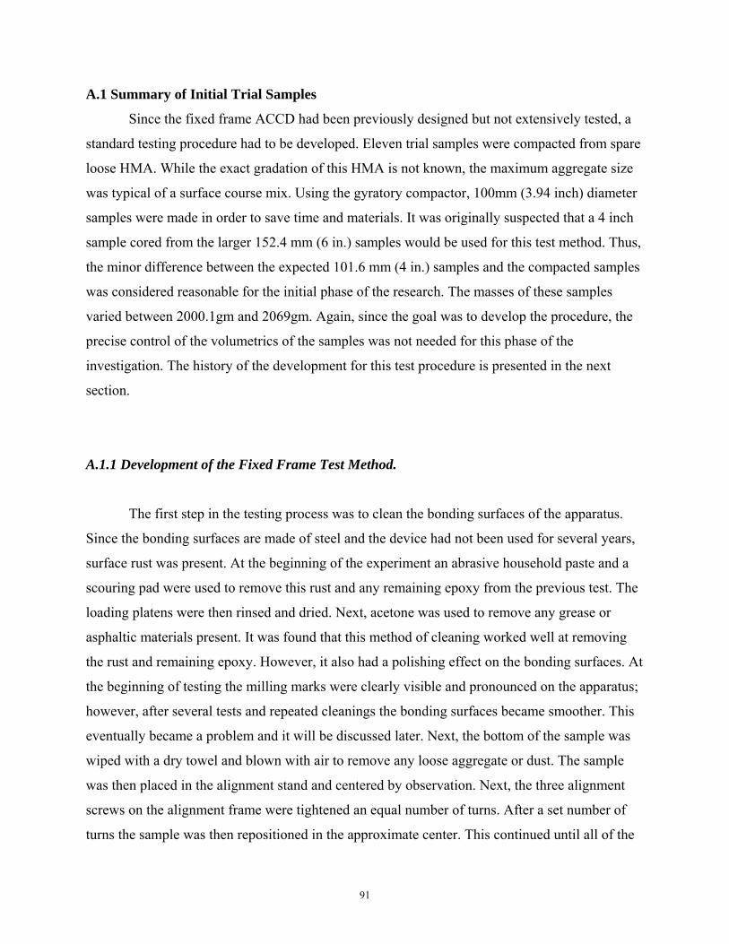
91

A.1 Summary of Initial Trial Samples

Since the fixed frame ACCD had been previously designed but not extensively tested, a

standard testing procedure had to be developed. Eleven trial samples were compacted from spare

loose HMA. While the exact gradation of this HMA is not known, the maximum aggregate size

was typical of a surface course mix. Using the gyratory compactor, 100mm (3.94 inch) diameter

samples were made in order to save time and materials. It was originally suspected that a 4 inch

sample cored from the larger 152.4 mm (6 in.) samples would be used for this test method. Thus,

the minor difference between the expected 101.6 mm (4 in.) samples and the compacted samples

was considered reasonable for the initial phase of the research. The masses of these samples

varied between 2000.1gm and 2069gm. Again, since the goal was to develop the procedure, the

precise control of the volumetrics of the samples was not needed for this phase of the

investigation. The history of the development for this test procedure is presented in the next

section.

A.1.1 Development of the Fixed Frame Test Method.

The first step in the testing process was to clean the bonding surfaces of the apparatus.

Since the bonding surfaces are made of steel and the device had not been used for several years,

surface rust was present. At the beginning of the experiment an abrasive household paste and a

scouring pad were used to remove this rust and any remaining epoxy from the previous test. The

loading platens were then rinsed and dried. Next, acetone was used to remove any grease or

asphaltic materials present. It was found that this method of cleaning worked well at removing

the rust and remaining epoxy. However, it also had a polishing effect on the bonding surfaces. At

the beginning of testing the milling marks were clearly visible and pronounced on the apparatus;

however, after several tests and repeated cleanings the bonding surfaces became smoother. This

eventually became a problem and it will be discussed later. Next, the bottom of the sample was

wiped with a dry towel and blown with air to remove any loose aggregate or dust. The sample

was then placed in the alignment stand and centered by observation. Next, the three alignment

screws on the alignment frame were tightened an equal number of turns. After a set number of

turns the sample was then repositioned in the approximate center. This continued until all of the

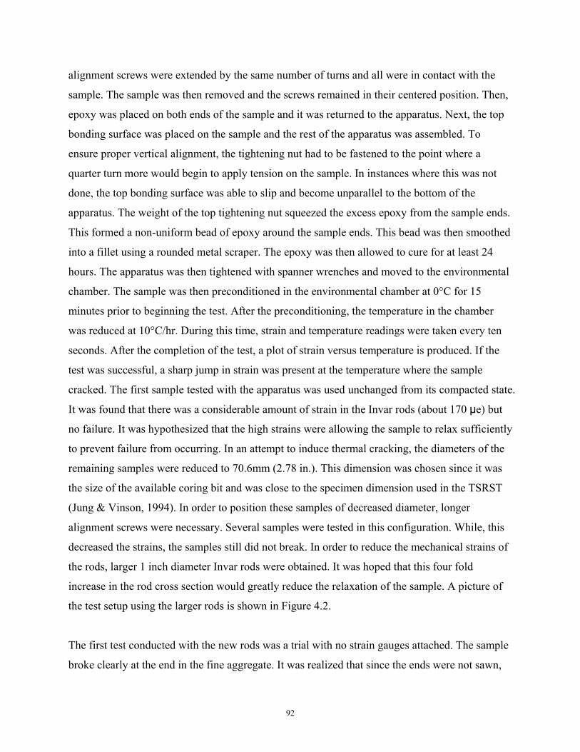
92

alignment screws were extended by the same number of turns and all were in contact with the

sample. The sample was then removed and the screws remained in their centered position. Then,

epoxy was placed on both ends of the sample and it was returned to the apparatus. Next, the top

bonding surface was placed on the sample and the rest of the apparatus was assembled. To

ensure proper vertical alignment, the tightening nut had to be fastened to the point where a

quarter turn more would begin to apply tension on the sample. In instances where this was not

done, the top bonding surface was able to slip and become unparallel to the bottom of the

apparatus. The weight of the top tightening nut squeezed the excess epoxy from the sample ends.

This formed a non-uniform bead of epoxy around the sample ends. This bead was then smoothed

into a fillet using a rounded metal scraper. The epoxy was then allowed to cure for at least 24

hours. The apparatus was then tightened with spanner wrenches and moved to the environmental

chamber. The sample was then preconditioned in the environmental chamber at 0°C for 15

minutes prior to beginning the test. After the preconditioning, the temperature in the chamber

was reduced at 10°C/hr. During this time, strain and temperature readings were taken every ten

seconds. After the completion of the test, a plot of strain versus temperature is produced. If the

test was successful, a sharp jump in strain was present at the temperature where the sample

cracked. The first sample tested with the apparatus was used unchanged from its compacted state.

It was found that there was a considerable amount of strain in the Invar rods (about 170 μe) but

no failure. It was hypothesized that the high strains were allowing the sample to relax sufficiently

to prevent failure from occurring. In an attempt to induce thermal cracking, the diameters of the

remaining samples were reduced to 70.6mm (2.78 in.). This dimension was chosen since it was

the size of the available coring bit and was close to the specimen dimension used in the TSRST

(Jung & Vinson, 1994). In order to position these samples of decreased diameter, longer

alignment screws were necessary. Several samples were tested in this configuration. While, this

decreased the strains, the samples still did not break. In order to reduce the mechanical strains of

the rods, larger 1 inch diameter Invar rods were obtained. It was hoped that this four fold

increase in the rod cross section would greatly reduce the relaxation of the sample. A picture of

the test setup using the larger rods is shown in Figure 4.2.

The first test conducted with the new rods was a trial with no strain gauges attached. The sample

broke clearly at the end in the fine aggregate. It was realized that since the ends were not sawn,

93

the sample was failing due to the concentration of fine aggregate particles on its end surfaces

during compaction. This caused a weak spot in the sample where failure was occurring. The rest

of the samples were sawn at both ends to eliminate this problem. When the sawn samples were

used, failure through the full diameter of the sample near the end was observed. Figure 4.3 shows

the results of this test. Based on the strain jump (average jump 64.9 με), it can be determined that

this crack occurred at around -25.6°C.

The next two tests failed at the bond between the epoxy and the metal. This was due to

the surface becoming polished from repeated cleanings. For sample 9, the surface was roughened

with 60 grit sandpaper. The surface was then cleaned with acetone and the sample epoxied to it.

Sample 9 broke through most of its diameter with a small semi circular shaped portion of the

epoxy breaking from the metal. Due to the strain jump (average jump 31.0 με), it can be

concluded that this crack occurred at around -25.2°C. After testing the remaining samples, it was

determined that this procedure was adequate at inducing measurable failure in the samples. Thus,

the following procedure was used for all remaining tests with this test method.

A.1.2 Fixed Frame Test Procedure

The final procedure determined from the 11 initial trial samples was as follows:

Sample preparation prior to conducting the test

1) Gyratory specimens must be compacted per specifications.

2) The samples must be cored using a coring bit and an apparatus to properly align and hold

the sample in place for coring. Field cores may also be used if the pavement layer

thickness is sufficient.

3) The ends of the cores must then be trimmed flat using a circular saw. It is vital to ensure

that both ends of the trimmed sample are smooth and parallel to one another.

94

The Test Procedure

4) After finishing the previous test, the bottom and top plate are heated to 150°C for about

two hours.

5) A metal scraper is used to remove most of the epoxy from the bonding surfaces.

6) The bottom and top platens must then be allowed to cool. Due to their high thermal mass

this takes several hours.

7) Acetone is then used to remove any asphalitc materials that may have melted on the

bonding surface.

8) Sixty Grit sandpaper is then used to remove any remaining epoxy and rust from the

bonding surface.

9) Acetone and paper towels are then used to remove the metal shavings left over from

sanding and to remove any grease or oils that may be present

10) Several minutes are allowed to ensure that all of the acetone has evaporated.

11) The sample ends are wiped and blown with air to ensure no loose aggregate or dust

remains on the sample.

12) The alignment frame (which consists of the small rods and alignment rings) is placed on

the bottom of the apparatus and the sample is aligned as described before.

13) The sample is removed and both ends are coated with epoxy.

14) The sample is placed back in the apparatus and the apparatus is completely assembled.

15) The excess epoxy is smoothed into a large fillet and allowed to cure for at least 24 hours.

16) The alignment frame is removed and the apparatus is assembled with the 1 inch diameter

instrumented test rods.

17) The test frame is tightened and placed in the chamber for 15 minutes at 0°C before

beginning the test.

18) The environmental chamber is cooled at a steady rate of 10°C/hr while a data acquisition

system records the strain in the Invar rods and the temperature every 10 seconds.

19) The results are plotted and the cracking temperature is determined from the temperature

where the jump in strain is observed.

95

APPENDIX B

STANDARD PROCEDURE FOR THE CONCENTRIC RING ACCD TEST

Figure B1. Schematics of ACCD

Pressing Head

Collar

Outer Mold

ACCD Ring

HMA Specimen

Base Plate

Collar

96

B.1.1 Preparation the Day Before the Test

1) Ensure that the outer ring and the Invar ring are clean. If they are soiled from a previous

test, clean them using kerosene. When cleaning the Invar ring, extreme care must be

taken to avoid splashing any kerosene on the inside of the ring, as it would likely have an

effect on the instrumentation. Clean other components of the apparatus only if they are

visibly soiled enough to cause problems with the normal conduction of the preparation

and testing procedures.

2) Cut paper disks to prevent the HMA from adhering to the base plate and the pressing

head.

3) If loose mix HMA is to be used batch the sample out into two pans of 3kg each for each

desired sample.

4) If laboratory mix HMA is to be used, prepare the aggregates and asphalt to be mixed

according to standard mixing procedures. It is advisable to batch out the dry aggregates

prior to the testing day of the test to save time and to prevent heat loss during the mixing

and compaction of the HMA sample.

B.1.2 On the Day of the Test

5) If using loose mix, place the pre-batched pans into the oven at the desired compaction

temperature. If using laboratory mix HMA, place the pre-batched aggregates, the asphalt

binder, and the stirrer in the oven at the desired mixing temperature.

6) Lubricate the Invar ring with Dow Corning High Vacuum Silicone Grease.

7) Assemble the apparatus as follows

a. Place the bottom paper disk on the base-plate.

b. Place the Invar ring in the center of the base-plate

c. Place the collar and the foil cap on the ring.

d. Place the outer ring and collar (if applicable).

8) Place the apparatus, pressing head, and spatula in the oven at the desired compaction

temperature and heat them for two hours.

9) If using loose mix HMA, skip to step six. If using laboratory mix HMA:

e. Remove the asphalt binder from the oven and mix with the stirrer.

97

f. Add the specified amount of asphalt binder to the aggregate and mix until the

aggregate is fully coated.

g. Weigh the total sample and split it into two equal pans.

10) Remove the apparatus from the oven.

11) Pour one of the pans of HMA into the apparatus.

12) Use the heated spatula to move the HMA to one half of the mold.

13) Place the other pan of HMA on the empty side of the mold.

14) Use the spatula to evenly distribute the HMA around the mold.

15) Use the spatula to rod the HMA 40 times.

16) Place the top paper disk in the mold on top of the HMA sample.

17) Place the pressing head in the mold on top of the top paper disk.

18) Place the apparatus in the press and align it.

19) Increase the displacement of the press until a 445 kN (100,000lb) load is reached. Once

this is achieved hold the displacement for 15 seconds then remove the load.

20) Repeat this process two more times.

21) Remove the apparatus from the press. Then, remove the pressing head, top paper disk,

and collar from the apparatus.

22) Set the apparatus aside; make a note of the time.

23) Perform steps 6-17 for the remainder of the samples to be compacted.

24) Turn the environmental chamber on and set it to 5°C. Prepare the Labview file to collect

test data at 10 second intervals.

25) After two hours from the time of compaction for each sample, place the pressing head on

top of the HMA sample and carefully flip the entire apparatus so that it is now sitting on

the pressing head with the base plate on top.

26) Remove the base plate and bottom paper. Use a heat gun to slightly heat up the paper so

it can be removed easily. Little heat application is needed to remove it.

27) Use the press and extraction frame to extract the test specimen.

28) Place the thin plate at the bottom of the sample, and simultaneously lift and flip the

sample so that it is now sitting right side up on the thin aluminum plate. Care must be

exercised in this step to avoid any stretching or distortion of the sample.

29) Place the sample in the environmental chamber and note the time.

98

30) After one hour remove the sample. Measure the desired notch length (38.1 mm or 1.5 in.)

and mark the area with a keel, ensuring that the mark is aligned with the strain gage.

31) Use a dry circular saw to cut the sample notch at the marked location and depth.

32) Place the sample back into the chamber and connect the ring instrumentation to the data

acquisition system.

33) Once all samples have been similarly cut, set the chamber to 0°C and start the data

acquisition system.

34) After one hour at 0°C begin the 10°C/hr temperature profile. At this time the test may be

tested overnight.

35) On the following day, measure the specimen air voids using the SSD method to

determine the bulk specific gravity as described in AASHTO T166

36) Take measurements of:

h. Cross section length: both top and bottom of the notch.

i. The inner height of the HMA ring at the strain gage

j. The outer height of the HMA ring at the strain gage

k. The minimum and maximum outer height of the HMA ring (optional).

37) Data analysis

l. Plot the temperature versus strain series obtained from the data acquisition system.

m. If a peak is present, draw a horizontal line at the peak value and a line tangential

to the linear portion of the strain versus temperature curve (this linear portion

occurs sometime after the initial stages of the test and before the crack begins to

form). The temperature where these two lines intersect is defined as the cracking

temperature.

38) If no peak is present, draw lines tangential to the initial linear portion and the final linear

portion of the strain versus temperature curve. The temperature where these two lines

intersect is defined as the cracking temperature.

99

APPENDIX C

MATERIALS USED

100

C1. Ohio DOT Mixes

Large quantities of ODOT field mixes were obtained and utilized in this project. These were

named respectively ODOT mix 1, 2, 3 and 4. For simplicity the mixes were labeled as OD-1,

OD-2, etc. Extensive data was available for these mixes and a data sheet was compiled for each

mix; these datasheets are presented below.

Table C-1 ODOT 1 Data Sheet ODOT 1 Data She

ODOT Job Number:

B447229

Design Method: Marshall

Gradation Mix Type Type 1 Sieve %

Passing Usage Surface

2" 100 Traffic Medium 1-

1/2" 100 %Binder Content @ Opt Air Voids 5.8 1" 100 Max Theoretical @ Optimum 2.452

3/4" 100 PG-Grade by Proposal 70-22 1/2" 100 % Virgin Binder 5.3 3/8" 97 Virgin Binder Grade 70-22

#4 56 Polymer Type SBS #8 39 Mixing Temperature (°F) 320

#16 25 Compaction Temperature (°F) 300 #30 17 % Air Voids 3.5 #50 10 VMA 16

#100 5 Critical Temperature (°C) -24.0 #200 2.8

Aggregate % by type weight Size Type ODOT

Gsb Coarse 49 #8 Limestone 2.652 Fine 35 703.05 Limestone Sand 2.633 Fine 6 703.05 Natural Sand 2.541 % AC RAP 10 5.44 LS/GR 2.653 Mix Gbs 2.639 et

101

Table C-2 ODOT 2 Data Sheet ODOT Job Number: B445222 Design Method: Marshall

Sieve 2"

Gradation % Passing 100

Mix Type Usage Traffic

Type 1 Surface Medium

1- 1/2" 1"

3/4" 1/2" 3/8" #4 #8

#16 #30

100 100 100 100 96 54 35 23 15

%Binder Content @ Opt Air Voids Max Theoretical @ Optimum PG-Grade by Proposal % Virgin Binder Virgin Binder Grade Polymer Type Mixing Temperature (°F) Compaction Temperature (°F) % Air Voids

5.9 2.388 64-

22 5.9

64-22 na 315 285 3.5

#50 8 VMA 16.5 #100 #200

4 3.9

Critical Temperature (°C) -23.2

Aggregate type Coarse

% by weight 55

Size #8 Type Limestone

ODOT Gsb 2.586

Fine 25 Sand Limestone 2.614 Fine 20 Sand Natural Sand 2.596

% AC RAP

Mix Gbs 2.595

102

Table C-3 ODOT 3 Data Sheet ODOT Job Number:

B445433

Design Method: Superpave

Gradation Mix Type A Sieve % Passing Traffic Normal

2" 100 # Gyrations @ Nini 7 1-1/2" 100 # Gyrations @ Ndes 65

1" 100 # Gyrations @ Nmax 105 3/4" 100 %Binder Content @ Opt Air Voids 5.7 1/2" 96 Max Theoretical @ Optimum 2.523 3/8" 89 PG-Grade by Proposal 76-22 #4 63 % Virgin Binder 5.2 #8 34 Virgin Binder Grade 76-22 #16 23 Polymer Type SBS #30 17 Mixing Temperature (°F) 330 #50 14 Compaction Temperature (°F) 310

#100 9 % Air Voids 4 #200 4.8 VMA 15.9

Critical Temperature (°C) -25.3

Aggregate % by type weight % Fractured Size Type ODOT Gsb

Coarse 20 100 Sp. 57 Stone 2.665 Coarse 20 100 8 Stone 2.673 Coarse 26 100 9 Stone 2.695

% FAA Fine 24 50.1 703.05 MFG Sand 2.799

% AC RAP 10 5.33 3/4" Millings 2.74

Mix Gbs 2.713

103

Table C-4 ODOT 4 Data Sheet ODOT Job Number:

Gradation

B447284

Design Method: Superpave

Sieve

2" 1-1/2"

1" 3/4" 1/2" 3/8" #4 #8 #16 #30 #50

#100

% Passing 100 100 100 100 97 85 57 40 24 15 8 4

Mix Type Traffic

# Gyrations @ Nini # Gyrations @ Ndes # Gyrations @ Nmax

%Binder Content @ Opt Air Voids Max Theoretical @ Optimum

PG-Grade by Proposal % Virgin Binder

Virgin Binder Grade Polymer Type

Mixing Temperature (°F) Compaction Temperature (°F)

% Air Voids

A Normal

7 65 105 5.9

2.458 70-22

5.4 70-22 SBS 320 300 4

#200 3.3 VMA 16.8 Critical Temperature (°C) -27.6

Aggregate type

% by weight

% Fractured

Size Type ODOT Gsb Coarse 25 100 7 Limestone 2.679

Coarse 19 100 8 Limestone 2.664

% FAA Fine 46 47.8 Sand Limestone 2.611

% AC RAP 10 5 RAP 2.701

Mix Gbs 2.670

104

RAP Mixes

A large quantity of loose HMA for low volume roadways (LV 404) was obtained from Flexible

Pavements of Ohio. Five of these mixes contained varying amounts of SBR polymer and

Recycled Asphalt Pavement (RAP). The sixth mix contained a different binder type than the rest.

Mixes were classified by their RAP content and their polymer percentage or binder type. Table

C-5 shows the names of the mixes and the Flexible Pavements of Ohio mix number.

Table C-5 RAP Mixes

Mix Type (LV 404) Flexible Pavements of Ohio (FPO) Mix Number

20% RAP 0% SBR 1

40% RAP 0% SBR 6

40% RAP 3% SBR 7

40% RAP 4% SBR 8

40% RAP 5% SBR 9

40% RAP PG 58-22

105

APPENDIX D

Implementation Plan

106

OHIO DEPARTMENT OF TRANSPORTATION OFFICE OF PAVEMENT ENGINEERING RESEARCH IMPLEMENTATION PLAN

Title: A Simple Test Procedure for Evaluating Low Temperature Crack Resistance of Asphalt Concrete State Job Number: 134260 PID Number: Research Agency: Ohio University Researcher(s): Sang-Soo Kim, Shad Sargand Technical Liaison(s): David Powers Research Manager: Monique Evans Sponsor(s): ODOT/FHWA Study Start Date: October 1, 2005 Study Completion Date: June 30, 2008 Study Duration: Study Cost: $101,795 Study Funding Type: 80/20 Federal/State from SP&R Part 2

STATEMENT OF NEED: Low temperature cracking is one of the major distress modes in asphalt pavement and is disastrous to pavement performance and service life. Currently, there are two approaches to characterize the low temperature thermal cracking potential of asphalt concretes; (1) mechanistic-empirical analysis (Superpave Indirect Tensile Creep and Strength Test, IDT) and performance model and (2) a torture test (Thermal Stress Restrained Specimen Test, TSRST). Both methods have been validated with field performance data and predict the low temperature cracking potential of asphalt concrete mixes. However, neither test can be readily used as a routine test because of the complex test and analysis procedures for IDT and the costly specialized equipment, and the difficulty producing beam specimens for TSRST. A new simple test procedure is needed to evaluate the low temperature cracking potential for a single severe freezing event and thermal fatigue for the environment and materials commonly used in Ohio. RESEARCH OBJECTIVES: • To determine coefficient of thermal expansion (CTE) of Ohio aggregates and mixes, • To develop a simple test procedure, as a part of a mix design system, to determine the thermal cracking

resistance of asphalt concrete mixes, • To validate the simple test device by laboratory testing, and • To determine the thermal cracking resistance of typical ODOT asphalt concrete mixes prepared with

local materials for the future validation of the new test device. RESEARCH TASKS:

• Determine coefficient of thermal expansion (CTE) of Ohio aggregates • Determine the role of aggregate CTE in asphalt pavement low temperature cracking • Develop a simple test procedure determining asphalt pavement low temperature cracking • Validate the simple test procedure

RESEARCH DELIVERABLES: Final Report, Executive Summary RESEARCH RECOMMENDATIONS: Asphalt Concrete Cracking Device (ACCD) is developed to determine the low temperature cracking potential of asphalt concrete. In ACCD test, by having asphalt concrete compacted around Invar ACCD ring, field condition is closely and easily simulated. The dissimilar CTEs of asphalt concrete and ACCD

107

ring induce tensile stress within the asphalt concrete and eventual crack under cooling. ACCD is more accurate, simpler, and faster test method than the currently available Thermal Stress Restrained Specimen Test (TSRST). Accuracy: The standard deviation of ACCD cracking temperature was less than 1°C for various mixes tested. Since the sample is molded on the testing device, ACCD ring, there is no alignment problem that commonly associated with TSRST procedure. It also minimizes the disturbance of the sample. Simplicity: One of the most cumbersome steps in asphalt concrete tension test is gluing. The ring shape of the specimen geometry eliminates the need for gluing. Since the tensile stress within asphalt concrete is induced by the difference in CTEs of asphalt concrete and ACCD ring, no other mechanical loading device is required which requires complicated controlling device and frequent calibration. Fast measurement: The elimination of gluing step shortens saves a day or more. Since no mechanical loading device is necessary, multiple specimens can be test at the same time.

PROJECT PANEL COMMENTS: IMPLEMENTATION STEPS & TIME FRAME: Through this research project, ACCD demonstrated its usefulness and easy to use test procedure. To be adopted in asphalt mix design procedure for ODOT, additional research and nationwide critical review of ACCD are needed. In the future research, the effects of asphalt binder properties, aggregate properties, and mix volumetrics on the low temperature cracking potential of asphalt concrete need to be studied with ACCD and compared with theoretical analysis. One of the outcomes of this research will be specific limit values to be used in mix design and analysis procedure to prevent the low temperature cracking of asphalt pavement. This type of research would take about 2 years. To receive nationwide review, several publications will be submitted to national conferences and peer-reviewed journals. A paper summarizing the development of ACCD is accepted for presentation and publication at 2010 Association of Asphalt Paving Technologists annual meeting. Presentation and discussion in FHWA’s Expert Task Group (ETG) Meeting is also planned. EXPECTED BENEFITS: For a paving project site, ACCD test can identify asphalt mix designs that potentially experience low temperature cracks and prevent them being used for construction. EXPECTED RISKS, OBSTACLES, & STRATEGIES TO OVERCOME THEM: ACCD is a new test method. Currently, there is no problem using ACCD to determine the relative ranks of asphalt concretes. However, ACCD is required to have field calibration. The ACCD cracking temperature needs to be compared with field cracking temperature and the relationship should be known. Accumulation of ACCD and field performance data for period of time will provide ACCD limit values to be used in future mix design process OTHER ODOT OFFICES AFFECTED BY THE CHANGE: PROGRESS REPORTING & TIME FRAME: TECHNOLOGY TRANSFER METHODS TO BE USED: Journal publication and conference presentation will be the main route for disseminating this new test device

108

IMPLEMENTATION COST & SOURCE OF FUNDING: For additional research, the possibility of utilizing FHWA’s Pooled Fund Study (PFS) will be considered. The low temperature thermal cracking is a common problem experienced by all northern states and Canadian provinces and there are significant interests in test device like ACCD. ODOT’s financial burden will be the amount of contribution that it will make toward the possible Pooled Fund Study. The additional cost to adopt ACCD in ODOT asphalt mix design process will be the cost of purchasing ACCD equipment.

Approved By: (attached additional sheets if necessary) Office Administrator(s):

Signature: Office: Date: Signature: Office: Date:

Division Deputy Director(s):

Signature: Division: Date:

Signature: Division: Date:

ORITE • 141 Stocker Center • Athens, Ohio 45701-2979 • 740-593-2476 Fax: 740-593-0625 •orite@bobcat.ent.ohiou.edu •http://webce.ent.ohiou.edu/orite/